Statistical Analysis of Cell Motion

by

Edward Luke Ionides

B.A. (Cambridge University) 1994M.A. (University of California, Berkeley) 1998

A dissertation submitted in partial satisfaction of the

requirements for the degree of

Doctor of Philosophy

in

Statistics

in the

GRADUATE DIVISION

of the

UNIVERSITY OF CALIFORNIA, BERKELEY

Committee in charge:

Professor David R. Brillinger, ChairProfessor David J. AldousProfessor George F. Oster

Summer 2001

The dissertation of Edward Luke Ionides is approved:

Chair Date

Date

Date

University of California, Berkeley

Summer 2001

Statistical Analysis of Cell Motion

Copyright 2001

byEdward Luke Ionides

1

Abstract

Statistical Analysis of Cell Motion

by

Edward Luke Ionides

Doctor of Philosophy in Statistics

University of California, Berkeley

Professor David R. Brillinger, Chair

Certain biological experiments investigating cell motion result in time lapse video mi-

croscopy data which may be modeled using stochastic differential equations. These

models suggest statistics for quantifying experimental results and testing relevant

hypotheses, and carry implications for the qualitative behavior of cells and for un-

derlying biophysical mechanisms. A state space model formulation is used to link

models proposed for cell velocity to observed data. Sequential Monte Carlo methods

enable parameter estimation and model assessment for a range of applicable models.

One particular experimental situation, involving the effect of an electric field on cell

behavior, is considered in detail.

There are several reasons why one might carry out parameter estimation by max-

imizing a smooth approximation to the likelihood in preference to the widely used

method of maximum likelihood. If the likelihood is approximated by Monte Carlo sim-

ulation then a smoothed approximation may be all that can reasonably be obtained.

If the likelihood function has many local maxima then a smooth approximation can

lead to a more tractable and possibly more appropriate maximization problem. A

theory for maximum smoothed likelihood estimation is developed using the frame-

work of local asymptotic normality (LAN). This property of LAN is demonstrated

for certain state space models whose state process is a diffusion process.

2

A complementary approach to direct observation of cell motion is to stain fixed

cells to determine the spatial distribution throughout the cell of a molecule of inter-

est. The data are digitized microscopy images. An algorithm is developed to quantify

relevant features of data collected as part of the investigation on the effect of electric

fields. Summary statistics and test statistics are proposed which are not model depen-

dent, requiring only the symmetry of the experiment for their validity, but which can

be justified in the context of a particular stochastic model for the staining process.

iii

To my father

iv

Here vigour failed the towering fantasy,Yet the will rolled onward like a wheel,In even motion, impelled by the loveThat moves the sun in heaven and the stars.

Dante Alighieri

v

Acknowledgements

I would like to thank Professor David Brillinger for his patient advice and support,

over many years and very many cups of coffee. The faculty, staff, computing facility

and fellow graduate students at the Statistics Department deserve thanks en masse for

creating a unique research environment. Professors Oster and Bickel and the late Pro-

fessor Le Cam provided influential discussion. My family encouraged me throughout

my Berkeley experience. Many friendships have sustained my studies, though some

deserve special mention. Eugene Miloslavsky and Maja Pavlic for helping me to move

house four times. Dave Johnson for being a role model of recovery from computer

injuries. Liza Levina for helpful and insightful conversations inside and outside of our

office. I am grateful for assistance in typing and data analysis from Von Bing Yap,

Gillian Ward, Jane Fridlyand and Faye Yeager.

vi

Contents

1 Introduction 11.1 Some Background to Cell Motion . . . . . . . . . . . . . . . . . . . . 21.2 Diffusion Processes and Stochastic Calculus . . . . . . . . . . . . . . 51.3 State Space Models . . . . . . . . . . . . . . . . . . . . . . . . . . . . 81.4 Models for Cell Shape . . . . . . . . . . . . . . . . . . . . . . . . . . 11

2 Statistical Analysis of Cell Motion 152.1 Models of Cell Translocation and Migration . . . . . . . . . . . . . . 162.2 Consequences and Applications . . . . . . . . . . . . . . . . . . . . . 21

2.2.1 Do kineses work? . . . . . . . . . . . . . . . . . . . . . . . . . 212.2.2 Model-based and model-free methods . . . . . . . . . . . . . 222.2.3 A model for galvanotaxis . . . . . . . . . . . . . . . . . . . . 24

2.3 Inference from Cell Tracking Data . . . . . . . . . . . . . . . . . . . . 262.4 Parameter Estimation for Models of Cell

Translocation . . . . . . . . . . . . . . . . . . . . . . . . . . . . . . . 322.5 A Statistical Analysis of Cell Shape . . . . . . . . . . . . . . . . . . . 37

3 Asymptotic Theory for Maximum Smoothed Likelihood Estimationand an Application to State Space Models 453.1 Maximum Smoothed Likelihood Estimation . . . . . . . . . . . . . . 483.2 Checking LAN for State Space Models . . . . . . . . . . . . . . . . . 583.3 Concluding Remarks . . . . . . . . . . . . . . . . . . . . . . . . . . . 64

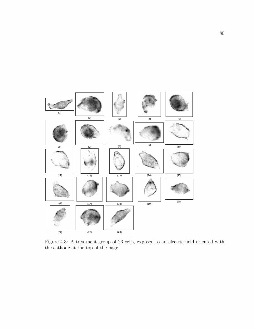
4 A Statistical Analysis of Data Arising from Staining Fixed Cells 664.1 Computation of the boundary and its staining . . . . . . . . . . . . . 684.2 Some statistics to measure stain location . . . . . . . . . . . . . . . . 734.3 A stochastic model . . . . . . . . . . . . . . . . . . . . . . . . . . . . 744.4 Analysis of some experimental data . . . . . . . . . . . . . . . . . . . 794.5 Conclusions . . . . . . . . . . . . . . . . . . . . . . . . . . . . . . . . 83

A Some Results on Conditional Differentiability in Quadratic Mean 85

vii

Bibliography 88

1

Chapter 1

Introduction

In this thesis we describe some problems in cell biology, some experimental mea-

surements made to investigate these problems, and some statistical tools suitable for

the analysis of the resulting data. The synergy from studying these two topics in

some detail in one thesis is that questions of substantive scientific interest serve as a

whetting stone to sharpen the statistical tools which leads in turn to improved data

analyses. In particular, Chapters 2 and 4 develop statistical analyses of data col-

lected on moving cells and fixed cells respectively. In these chapters, relevant existing

statistical techniques are assembled to address particular scientific questions. Chap-

ter 3 investigates a gap in the existing theory for statistical inference for some of the

models proposed in Chapter 2. The resulting theory complements Chapter 2, while

also making a contribution to many other data analyses for which similar statistical

methods are applicable.

The central approach to Chapter 2 is to use stochastic differential equations

to define parametric families of models whose parameters have physical interpre-

tation. This approach was pioneered in (Kendall, 1974; Levin, 1986; Brillinger, 1997;

Brillinger and Stewart, 1998). In the situation studied here, we are led toward a

so-called state space model by the consideration that we model cell velocity and ob-

serve cell location at discrete times with some measurement error. A convenient way

to find parameter estimates and their uncertainties in state space models turns out

to be approximating the likelihood function using the method of sequential Monte

2

Carlo simulation developed by Kitagawa (1996). It is then tempting to estimate the

likelihood function by applying a statistical smoothing technique to the Monte Carlo

estimates of the likelihood at different parameter values. Chapter 3 develops some

theory which suggests that using a smooth approximation to the likelihood function

is a reasonable thing to do. It further demonstrates situations where it is appro-

priate to smooth the likelihood function deliberately. This framework is then used

to find asymptotic properties of estimators for certain state space models, when the

underlying state process is a diffusion.

In Chapter 4 an algorithm is constructed, using standard tools of image analysis

and statistics, to quantify experimental data consisting of images of fixed cells stained

for a particular protein. Summary statistics and tests of relevant hypotheses are

presented, and then found to arise naturally from a statistical model. The methods

are next demonstrated on some available data. The model can be seen from the data

to be reasonably appropriate.

The remaining sections of this chapter give some background material to lay the

foundations for the subsequent chapters. Section 1.1 gives an overview to cell motion,

and Sections 1.2, 1.3 and 1.4 outline some results for stochastic differential equations,

state space models and stochastic models for cell shape respectively.

1.1 Some Background to Cell Motion

Active migration of blood and tissue cells is essential to a number of physiolog-

ical processes such as inflammation, wound healing, embryogenesis and tumor cell

metastasis (Bray, 1992). It also plays an important role in the functioning of many

bioartificial tissues and organs (Langer and Vacanti, 1999), such as skin equivalents

(Parenteau, 1999) and cartilage repair (Mooney and Mikos, 1999). Modern tech-

niques in microscopy, genetics and pharmacology helped to make some progress in

unraveling the complex biophysical processes involved in cell motion (Maheshwari

and Lauffenburger, 1998). Although different cell types show diverse methods of

locomotion, there are general principles that are widely applicable for cells moving

along a substrate. First a cell extends a protrusion by actin filament polymerization

3

(Mogilner and Oster, 1996), which then attaches to the substrate using integrin adhe-

sion receptors (Huttenlocher et al., 1995). A contractile force is next generated which

moves the cell body. Finally the cell must attach from the substrate at its trailing

end.

Various mathematical models incorporating the above principles of cell motion

have been proposed. The most ambitious of them attempt to represent all the phys-

ical and chemical processes involved in the motion of an entire cell (Tranquillo and

Alt, 1996; Dickinson and Tranquillo, 1993; Dembo, 1989). Others concentrate on

a specific process such as extension of a protrusion (Mogilner and Oster, 1996) or

receptor dynamics (Lauffenburger and Linderman, 1993). The primary purpose of

these biophysical models is to demonstrate that the proposed mechanisms can in fact

produce the forces and behaviors observed experimentally.

Another approach to modeling cell motion is phenomenological in nature. The

so-called correlated random walks of Alt (1980), Dunn and Brown (1987) and Shen-

derov and Sheetz (1997) have been proposed to describe observations of isolated cells

locomoting on a substrate. For applications, the behavior of cell populations may be

of more direct interest, and here diffusion approximations to population behavior are

widely used, for example in Ford et al. (1991). The theoretical relationships between

single cell models and population models are studied in Alt (1980), Dickinson and

Tranquillo (1995), Ford and Lauffenburger (1991). An empirical comparison between

single cell and cell population models is given in Farrell et al. (1990). Phenomeno-

logical models are used for quantifying experimentally observed cell behavior, and

do not require justification in terms of a proposed mechanism. Nevertheless the line

dividing biophysical from phenomenological models is in fact only a difference in com-

plexity, and can become blurred as even the simpler phenomenological models can

have implications concerning underlying biophysical mechanisms (Dunn and Brown,

1987).

The questions of scientific and engineering interest about cell motion can be

broadly summarized into the following: What biophysical processes are involved in

cell motion? How can the speed and direction of the motion be modeled? One ap-

proach toward answering these questions is to collect temporal sequences of images of

4

moving cells. This is the data type that will be considered in later chapters. Various

experimental protocols for studying cell motion are discussed in Alt, Deutsch and

Dunn (1997) and Alt and Hoffmann (1990). Cells may be observed moving sepa-

rately on a microscope slide, or in a three-dimensional collagen gel. The cells under

investigation may be connected to form a tissue, with a stain used to identify and

track groups of cells.

Computer-assisted microscopy can be used to build three-dimensional images of

moving cells (Murray et al., 1992; Wessels et al., 1994). Traction forces can be

measured by observing the wrinkles produced by a cell moving on an elastic substrate

(Oliver et al., 1995). The particular experimental procedure that will recur repeatedly

as an example in this thesis is described in more detail in Example 1 below. It is an

investigation of the reaction to a stimulus of single cells locomoting on a microscope

slide using time-lapse observations. Analysis of this relatively simple cell motion

experiment can be taken as motivation for the theory developed in Chapters 2, 3 and

4.

Example 1. Investigation of Galvanotaxis. Human keratinocytes (skin cells) migrate

toward the negative pole in direct current electric fields of physiological strength. This

phenomenon is termed galvanotaxis and is of particular interest in wound healing

(Nishimura et al., 1996). It has also recently become a tool for more general study

of directional cell motility, as in Fang et al. (1999). One of the challenges in practice

of investigating directional response to a stimulus is to set up experimentally the

controlled, uniform gradients required for clear and reproducible results. However,

such gradients are relatively easy to attain for DC electric fields, making galvanotaxis

a convenient model system for investigating basic aspects of directional cell motility.

The data analyzed in Section 2.2 were collected by Dr. Kathy Fang at University

of California, Davis, to investigate the effect of calcium ion (Ca2+) concentration on

galvanotaxis. The experimental method is similar to that used in Fang et al. (1999)

to demonstrate the role of the epidermal growth factor receptor (EGFR) in galvan-

otaxis. Specifically, normal human keratinocytes from neonatal foreskin epidermis

were cultured and plated onto a glass coverslip coated with extra-cellular matrix (col-

5

lagen). The treated coverslip was placed in a galvanotaxis chamber as described in

Nishimura et al. (1996). Cells were then observed using phase contrast or differential

interference contrast optics with video images being digitally captured. The images

were typically captured at intervals of ten minutes, during a one hour observation

period, resulting in seven images per experiment. Further details of the experimental

method are given in Fang et al. (1999).

1.2 Diffusion Processes and Stochastic Calculus

A stochastic process X(t), t ∈ R is said to be an m-dimensional diffusion process

if it has continuous sample paths in Rm and possesses the strong Markov property,

that for a stopping time τ , X(t), t ≥ τ is conditionally independent of X(t), t ≤ τgiven Xτ . The treatment here draws on results in Oksendal (1998) and Stoock and

Varadhan (1979), and is based on the approach in Karlin and Taylor (1981) which

however deals only with diffusion processes with sample paths in R.

Definition. The infinitesimal mean, or drift, of a diffusion process X(t) is

µ(x, t) = limh↓0

(1/h)E[X(t + h)−X(t) | X(t) = x],

and the infinitesimal variance is

Γ(x, t) = limh↓0

(1/h)E[(X(t + h)−X(t))(X(t + h)−X(t))T | X(t) = x],

when these limits exist. Here the superscript “T” refers to the operation of matrix

transposition.

A remarkable property is that the law of a diffusion process is specified by µ(x, t)

and Γ(x, t) provided the limits exist, excepting behavior at any boundary and assum-

ing a higher moment condition that for some r > 2 and all x and t

limh→0

(1/h)E[|X(t + h)−X(t)|r | X(t) = x] = 0.

Examples are Brownian motion in R1, with µ(x, t) = 0 and Γ(x, t) = σ2, and the

Ornstein–Uhlenbeck process, with µ(x, t) = −αx and Γ(x, t) = σ2.

6

We will be concerned with diffusion processes as the solutions to certain stochastic

differential equations (SDEs) of the form

dX(t) = b(X(t), t)dt + γ(X(t), t)dW (t), (1.1)

where b(X(t), t) is a vector in Rm, γ(X(t), t) is an m × m matrix and W (t) is a

standard Brownian motion in Rm, i.e., a diffusion process with infinitesimal drift

of zero and infinitesimal variance I. There is more than one way to give a formal

meaning to the infinitesimal equation (1.1), leading to different possible solutions.

The Ito solution is written

X(t) = X(0) +

∫ t

0

b(X(s), s)ds +

∫ t

0

γ(X(s), s)dW (s)

where integration is carried out using the so-called Ito integral. The Ito integral is

defined, for a stochastic process Y (t), t > 0, when the limit exists, as

∫ t

0

Y (s)dW (s) = limN

N−1∑n=0

Y (tn)(W (tn+1)−W (tn)).

The limit is taken over all sequences of partitions whose largest intervals tend to zero,

in other words, over collections ti, i = 1, 2, . . . , N with 0 = t0 < t1 < · · · < tN = t

and supn |tn+1 − tn| → 0. An alternative interpretation, the Stratonovich solution, is

written

X(t) = X(0) +

∫ t

0

b(X(s), s)ds + S−∫ t

0

γ(X(s), s)dW (s)

where integration is carried out using the Stratonovich integral defined as

S−∫ t

0

Y (s)dW (s) = limN−1∑n=0

[(1/2)(Y (tn) + Y (tn+1))(W (tn+1)−W (tn))].

For the Ito integral, a key part of the definition is that the argument tn of Y (·) is

not in the interval (tn, tn+1). The Stratonovich integral acquires a more symmetric

appearance by replacing Y (tn) with 12(Y (tn) + Y (tn+1)). However, since Y (tn+1)

depends itself on W (t), tn ≤ t ≤ tn+1, the Stratonovich integral can be interpreted

as looking infinitesimally into the future. The Stratonovich integral has been reported

as being more appropriate for modeling phenomena in the physical world than its Ito

counterpart (Brillinger, 1997; Karlin and Taylor, 1981).

7

The Ito solution is a diffusion with infinitesimal coefficients µ(x, t) = b(x, t) and

Γ(x, t) = γ(x, t)γT (x, t). The Stratonovich solution is also a diffusion, but with

infinitesimal coefficients µi(x, t) = bi(x, t) + (1/2)∑m

j=1

∑mk=1

∂γij

∂xkγkj and Γ(x, t) =

γ(x, t)γT (x, t). Section 2.2 gives an example of a situation where the difference be-

tween the Ito and Stratonovich solutions becomes a relevant scientific issue.

Two results we mention here for use later are Ito’s lemma, which explains how the

infinitesimal coefficients change under a transformation of variables, and the Girsanov

theorem, which enables calculation of the likelihood ratio of diffusion processes when

this ratio exists.

Theorem 1.1 (Ito’s lemma) Let X(t) be the Ito solution to

dX(t) = b(X(t), t)dt + γ(X(t), t)dW (t).

For g(x) a twice continuously differentiable function Rm → R and Y (t) = g(X(t)),

under mild regularity conditions Y (t) satisfies the infinitesimal equation

dY (t) =∑

i

∂g

∂xi

(X(t))dXi(t) +1

2

∑ij

∂2g

∂xi∂xj

(X(t))dXi(t)dXj(t),

where dWi(t)dWj(t) = 1i=jdt and dWi(t)dt = dtdWi(t) = 0. Sufficient regularity

conditions are that for all i, j

P

[∫ t

0

|bi(X(s), s)|ds < ∞ for all t ≥ 0

]= 1

P

[∫ t

0

(γ(X(s), s)γT (X(s), s))ijds < ∞ for all t ≥ 0

]= 1.

The following version of the Girsanov theorem is based on Oksendal (1998, The-

orem 8.6.5), restated in a form convenient for the statistical inference application to

be presented in Chapter 2.

Theorem 1.2 (The Girsanov Theorem) Let X(t) ∈ Rm be the Ito solution to

dX(t) = b(X(t), t)dt + γ(X(t), t)dW (t),

8

with γ(X(t), t) an invertible m×m matrix. Under regularity conditions, the law PT

of X(t), 0 ≤ t ≤ T has a density with respect to the law QT of the Ito solution for

0 ≤ t ≤ T of

dX(t) = γ(X(t), t)dW (t).

This density gT is then a real-valued functional on functions [0, T ] → Rm which

are continuous with finite quadratic variation, and is given by the expression

gT (x) = exp

(∫ T

0

bT (x(s), s)(γ(x(s), s)γT (x(s), s))−1dx(s)

−1

2

∫ T

0

‖γ−1(x(s), s)b(x(s), s)‖2ds

).

A sufficient regularity condition is that

E[exp

(1

2

∫ T

0

‖γ−1(X(s), s)b(X(s), s)‖2ds

)]< ∞.

¤

Often the SDE (1.1) will not have an algebraic solution, but the SDE can then

often be approximately solved numerically. The simplest numerical technique, the

stochastic Euler method, sets

X((n + 1)δ) = X(nδ) + δb(X(nδ), nδ) +√

δγ(X(nδ, nδ))εn (1.2)

for some small δ > 0 and with εn ∼ N [0, I]. The notation used here, and subsequently,

is that N [µ, Γ] corresponds to a normal distribution whose mean is µ and whose co-

variance matrix is Γ. More elaborate techniques are available, based on stochastic

Taylor series expansions and implicit methods, similar to those for ordinary differen-

tial equations (Kloeden et al., 1992). For the requirements of this thesis, the Euler

method appeared to be adequate.

1.3 State Space Models

The general setup for a state space model consists of a so-called state process

Xn, n = 1, . . . , N which is a Markov chain taking values in a state space X , and

9

an observation process Yn = fn(Xn, εn), where εn is a sequence of independent

random variables taking values in E and fn : X × E → Y . Here Y is called the

observation space. In particular applications, the sets X , Y and E are often either

discrete (finite or countable) or subsets of some metric space.

State space models occur naturally in many scientific and engineering problems.

In the case that X is a discrete or countable set, a state space model is called a

hidden Markov model (HMM). HMMs are widely used in applications such as speech

recognition (Rabiner, 1989) and locating genes associated with diseases (Lander and

Green, 1987). In the case that (Xn, Yn) is a Gaussian process and X , Y , E are

Euclidean spaces, a state space model arises in the so-called LQG model central

to control theory (Whittle, 1996). It appears that real world phenomena are often

well modeled by some Markov process with sufficiently rich state space, perhaps

constructed according to physical or chemical or economic principles, about which we

can make only incomplete or noisy observations. This corresponds to the situation,

suggested by the terminology introduced, where we record the observation process

and are interested in understanding the behavior of the unobserved state process

conditional on the observation process.

The general treatment of state space models described here is based on Kitagawa

(1996). No algebraic structure is required on X , Y and E but we do assume that all

required densities exist with respect to some appropriate measures on these spaces.

The basic problems of state space models are prediction, filtering and smoothing.

These may be described as:

Prediction: Find the conditional density p(xn | y1, . . . , yn−1), of Xn given observa-

tions up to time n− 1.

Filtering: Find p(xn | y1, . . . , yn).

Smoothing: Find p(xn | y1, . . . , yN) for n < N .

A fourth related problem of particular interest to statistical inference is

Likelihood: Find the density of the complete observation sequence, p(y1, . . . , yN).

These problems can be solved in O(N) computational time, given the initial den-

10

sity p(x0), using the following recursion equations for prediction and filtering

p(xn | y1, . . . , yn−1) =

∫

Xp(xn−1 | y1, . . . , yn−1)p(xn | xn−1)dxn−1 (1.3)

p(xn | y1, . . . , yn) =p(xn | y1, . . . , yn−1)p(yn | xn)

p(yn | y1, . . . , yn−1)(1.4)

p(yn | y1, . . . , yn−1) =

∫

Xp(xn | y1, . . . , yn−1)p(yn | xn)dxn. (1.5)

The smoothing problem can then be solved by noting that

p(xn | y1, . . . , yN) ∝ p(xn, yn, yn+1, . . . , yN | y1, . . . , yn−1)

= p(yn, . . . , yN | xn)p(xn | y1, . . . , yn−1)

where p(yn, . . . , yN | xn) can be calculated by recursively applying the prediction and

filtering operations backwards, starting at time N , namely

p(yn, . . . , yN | xn) = p(yn | xn)p(yn+1, . . . , yN | xn)

p(yn+1, . . . , yN | xn) =

∫p(yn+1, . . . , yN | xn+1)p(xn+1 | xn)dxn+1.

The likelihood problem is solved using the quantities calculated in (1.5):

p(y1, . . . , yN) =N∏

n=1

p(yn | y1, . . . , yn−1).

For the hidden Markov model with finite state space, the integrals in the recursion

equations become sums which may be evaluated exactly. In the linear-Gaussian case

there is a closed form solution called the Kalman filter (Box and Jenkins, 1970).

In most other cases numerical approximations must be used to solve the recursion

equations. A popular method is to make a linear, Gaussian approximation to the

actual model. This approximation, termed the Extended Kalman Filter, often works

surprisingly well in practice. There are also several numerical approaches that aim to

solve approximately the exact recursion equations, rather than solving exactly some

approximating equations. Numerical integration can be used (Kitagawa, 1987) to

calculate approximately the integrals in (1.3) and (1.5). Monte Carlo Markov chain

methods (Carlin et al., 1992) and importance sampling (Durbin and Koopman, 2000)

11

provide other alternatives. The approach used for the data analysis in Chapter 2

is the sequential Monte Carlo method (Kitagawa, 1996), also known as the Particle

Filter.

To describe sequential Monte Carlo, suppose that at time n we have J random

particles X(f)n,1 , . . . , X

(f)n,J whose marginal distributions approximate the solution to the

filtering problem at time n corresponding to the density p(xn | y1, . . . , yn). The

prediction problem at time n + 1 is then approximated by the marginal distribution

of X(p)n+1,j obtained by moving particle X

(f)n,j according to the transition probabilities

of the state space Markov chain, i.e., draw X(p)n+1,j from p(xn+1 | xn = X

(f)n,j ). The

filtering problem at time n+1 is approximated by the marginal distribution of X(f)n+1,j

obtained by resampling the particles X(p)n+1,j, 1 ≤ j ≤ J with weights proportional

to the conditional likelihood given Yn+1, i.e., set X(f)n+1,j = X

(p)n+1,k with probability

p(Yn+1 | X(p)n+1,k)

/J∑

l=1

p(Yn+1 | X(p)n+1,l) .

This recursive definition of X(f)n,i and X

(p)n,i corresponds to an approximate solution

to equations (1.3) and (1.4). Del Moral (1996) shows that this approximation error

tends to zero as the number J of particles increases. Del Moral and Guionnet (1999)

find a central limit theorem for this convergence. The likelihood can then be estimated

via

p(yn | y1, . . . , yn−1) =1

J

J∑j=1

p(yn | X(f)n,j ).

For many applications, including some of the situations encountered in Chapter 2,

a linear state space model is adequate. In this case, a state space model is equiva-

lent to the much used ARMA model described in Box and Jenkins (1970), with an

implementation in S-Plus described in Venables and Ripley (1995).

1.4 Models for Cell Shape

In this section, a sequence of mathematical descriptions of cell shape is introduced

with decreasing generality and increasing simplicity. The ability of these models

12

to describe features of interest for scientific research is discussed. In Section 2.4

particular parametric forms are suggested and a data analysis presented.

Some previous work has studied cell shape more indirectly than is done in this

thesis. Dunn and Brown (1990) use moments to quantify cell shapes, but comment on

the difficulty of interpreting third and higher order moments. Noble (1990) calculates

a skeleton spanning the shape of a cell in order to identify lamellipodia. Soll et al.

(1997) describe a three-dimensional dynamic image analyzing system which computes

“more than 100 parameters of motility and dynamic morphology”. Writing down a

formal stochastic model can help by identifying appropriate parameters, showing rela-

tions between the parameters and making efficient use of available data for statistical

inference. Some pitfalls in using an assorted collection of parameters to quantify

and describe shapes, without an appropriate model, are discussed in Freedman et al.

(1998, Section 12.3).

The field of statistical shape theory, surveyed in Small (1996), defines the shape

of an object, data set or image as the total of all information that is invariant under

translations, rotations and isotropic rescalings. In our situation, symmetries of the

experiment may or may not lead to translation and rotation invariance. For example,

motion in a uniform electric field should have the same symmetries as the field itself,

namely translation but not rotation invariance. The idea of invariance to isotropic

rescaling is appealing. Each cell could then have its own scale and behave in the

same way up to its scale factor. Whether this assumption is justified in practice will

be decided by the data. At any rate, we do not intend to be restricted by the above

definition of Small (1996).

We suppose the interior of a cell at time t is given by a subset St of Rn, giving rise

to a shape process S = St, 0 ≤ t ≤ T. Usually n is either 2 or 3. If one supposes

that S takes a value which is a closed (or equivalently, open) subset of Rn× [0, T ] then

S can be formally constructed as a stochastic process using the methods of Matheron

(1975). In this general form, St could be a disconnected subset of Rn, which is a

biologically plausible possibility as the cell may divide or may leave some part of

itself behind, stuck on the substrate, when it moves. However we might ignore these

complications and suppose that St is a continuous deformation of S0, which is in turn

13

a continuous deformation of the unit ball in Rn. St is then said to be homotopic to

the unit ball. This means that S can be represented as the image of a shape function

s : Bn × [0, T ] → Rn (1.6)

where Bn = x ∈ Rn : |x| ≤ 1, the unit ball, and where s(·, ·) is continuous

in space and time. A reference for the topological terms and results used in this

section is Hocking and Young (1961). St is defined to be the image of s(·, t), which

makes St closed, compact and connected. The parameterization is far from unique, as

many different shape functions give the same image. A natural way of constructing

a shape function is for s(x, t) to give the position at time t of an imaginary particle

attached to the cell at time t = 0 and position s(x, 0). In experimental situations,

the imaginary particle can be replaced by a small bead which allows observation

of the local movement of the cell cytoplasm or membrane (Anderson et al., 1996).

Depending on the coating applied to a bead, it can either stay attached to the surface

of the cell membrane or undergo endocytosis. The shape function defined in this

natural way contains more information than the shape process alone. One feature of

interest that it can describe is the ruffling of a lamella. The leading edge of the cell

may fold on itself, causing a so-called ruffle (Hinz and Brosteanu, 1997). This results

in the shape function being not one to one as its image must fold back on itself.

Another approach is to model the boundary of the cell in terms of a boundary

function

b :∑n−1

×[0, T ] → Rn

where∑

n−1 = x ∈ Rn : |x| = 1, the unit n-sphere embedded in Rn, and b(·, ·) is

continuous in space and time. Supposing that b(·, t) is one to one, it defines a topo-

logical transformation, or homeomorphism, of the sphere. It is more appropriate to

think of topological rather than homeotopic mappings as models of cell boundaries,

as the former preserve the sense of inside and outside, by the Jordan–Brouwer separa-

tion theorem. The boundary function retains the interpretation of the shape function

in terms of the motion of particles attached to the cell surface if there is no ruffling or

recycling of the cell membrane. A further assumption, which produces an attractively

14

simplified model, is to suppose that the boundary function has a center-radius form.

For the case n = 2, appropriate for many microscopy images, this means that the

boundary function has the form

b(x, t) = c(t) + r(θ, t)x

where x = (cos θ, sin θ)T . This restrictive form is adequate for cell types that are

near convex in shape, such as keratinocytes, fish keratocytes and Xenopus mesoderm.

It is not so suitable for some other commonly studied cell types such as fibroblasts

and PMN (human polymorphonuclear white blood cells). The center, c(t), may be

an arbitrary measure of cell location. A convenient specification of the center is the

centroid, defined as

c(t) =

∫

St

xdS

∫

St

dS

−1

.

When observing a two-dimensional image, the centroid may be far from the true

center of mass of the cell as cell thickness varies enormously between the thick cell

body and the thin lamella. If the cell body can be clearly distinguished from the

image, its centroid may be closer to the center of mass.

A well-studied statistical problem requiring stochastic shape models is Bayesian

object recognition. The object of interest is modeled by a prior distribution on some

shape space. The shapes considered may be deformations of a template incorporating

knowledge of the form of the objects being looked for (Grenander and Keenan, 1993)

or may be a space of random polygons used to detect boundaries of arbitrary objects

(Pievatolo and Green, 1998). These prior distributions are candidate models for cell

shapes. For example, Grenander and Manbeck (1993) model potatoes using defor-

mations of an ellipse coming from a multivariate von Mises distribution. Grenander

and Miller (1994) model mitochondria using a polygon whose edge vectors are multi-

variate normal. Many other objects such as hands, brains and stomaches have been

modeled in similar ways.

15

Chapter 2

Statistical Analysis of Cell Motion

Studies involving observation of cell motion may be categorized, as in Dickinson

and Tranquillo (1995), by the length and time scales under primary consideration. On

the scale of locomotion the basic actions of cell motion are apparent: this is the scale on

which a cell may extend individual protrusions (broad lamellae, thinner lamellipodia

or hairlike filopodia) that can be used to pull itself along. On a longer time and length

scale, termed translocation, one observes the displacement of the cell due to one or

several motion cycles. As the resolution of detail about the motion decreases, gross

tendencies such as directional preferences can become more apparent. On the scale of

migration, the cumulative effect of many motion cycles is observed. Although on the

migration scale one loses the ability to observe directly the mechanisms of cell motion,

it is the behavior of cells on this scale which is of primary interest in applications,

such as development, cancer metastasis, and tissue engineering. Furthermore, some

assays such as the Boyden diffusion chamber (Byrne et al., 1998) entail observations

of populations of cells for which only the behavior on the migration scale can be

directly observed. Dickinson and Tranquillo (1995) develop mathematical methods

to relate models on different scales, using the method of adiabatic elimination of fast

variables (Gardiner, 1983).

The Keller–Segel model of chemotaxis (Keller and Segel, 1971; Byrne et al., 1998)

gives a widely accepted approach for modeling cells on the migration scale, using

Fokker–Planck equations. These models can be written as stochastic differential equa-

16

tions, and are discussed in Section 2.1. Section 2.1 also gives a thorough discussion

of models for translocation, using methods based on stochastic differential equations

to develop qualitative and quantitative understanding of these models. Section 2.2

discusses some situations where the models introduced in Section 2.1 clarify and con-

tribute to questions of scientific interest. Section 2.3 addresses hypothesis testing, and

Section 2.4 parameter estimation for the models of Section 2.1. Section 2.5 presents

an investigation of cell motion on the scale of locomotion.

2.1 Models of Cell Translocation and Migration

In this section we look at some models which quantify concepts arising in the

studies of cell motion discussed in Section 1.2. Each model describes the vector-

valued position or velocity of a single cell moving in the plane. The reader is asked

to suspend skepticism about the validity of these models until Section 2.2, where

it is indicated how such models may be used to help rather than hinder scientific

understanding even with the assurance that none provides a true representation of

reality. Also, we will look at ways to quantify the concepts of biological interest in

ways that do not rely on the validity of a particular model.

When the distribution of the velocity process has rotational symmetry about the

origin, and does not depend on position, the model is called isotropic. Such models,

suitable when the cell experiences no directional stimuli, are discussed first. When

the velocity process has directional asymmetry or depends on position then the cell is

said to perform taxis. The cell must then be picking up some locational or directional

cue from its environment.

Two characteristics used to describe isotropic cell motion are speed and persis-

tence. The story is that in the short term cells are observed to move with slowly

varying direction and speed. After a while they appear to forget their initial ori-

entation. This time scale is termed the persistence of the cell. The main model

for isotropic translocation in the literature is the so-called correlated random walk

(Alt, 1990; Dunn, 1983) where the velocity vt = (vx(t), vy(t)) follows an Ornstein–

Uhlenbeck process. This process is defined by the stochastic infinitesimal equation

17

(see Section 1.2)

(M1) dvt = −avtdt + bdWt

for positive constants a and b and a two-dimensional Brownian motion Wt. The

coefficient −avt is called the infinitesimal drift and b2 the infinitesimal variance.

Heuristically, a gives the rate at which the velocity regresses to zero and b gives the

magnitude of the random innovations which tend to push the velocity away from

zero. The root mean square speed can be calculated as√

b2/a, and a measure of

persistence is 1/a. One feature sometimes observed for cells is that their direction of

motion changes most rapidly when their speed is small (Shenderov and Sheetz, 1997).

This behavior is a property of (M1), as is most clearly seen by transforming to polar

coordinates (rt, θt) for the velocity by applying Ito’s lemma (Section 1.2). This leads

to the infinitesimal equations

drt =

(−art +

b2

2rt

)dt + bdW

(r)t

dθt =

(b

rt

)dW

(θ)t

for two independent one-dimensional Brownian motions W(r)t and W

(θ)t . In Shenderov

and Sheetz (1997) it is also observed that for some cell types the velocity has an

oscillatory behavior, with high correlation between velocities at certain time lags.

They propose a model

(M2) dvt =

(−avt − c

∫ t

−∞vse

−k(t−s)ds

)dt + bdWt,

where the evolution of the velocity process depends on the past values of the process.

Shenderov and Sheetz show that (M2) has oscillatory behavior for 4c > (a − k)2 in

the sense that the solutions to the related ordinary differential equation

dx

dt+ ax(t) + c

∫ t

0

x(s)e−k(t−s)ds = 0, t ≥ 0

are oscillatory. (In fact they miscalculate by a factor of√

2π, but we have not repro-

duced their error.) A natural probabilistic approach to generalizing (M1) to include

18

oscillatory behavior is to notice that (M1) is in the form of a continuous time autore-

gressive model of first order, CAR(1), studied in Jones (1981). The CAR(2) model is

the solution to the coupled equations

(M3)dvt = vtdt

dvt = (−αdvt − βvt)dt + bdWt.

One can rewrite (M2) to look more like (M3) by setting ut =∫ t

−∞ vse−k(t−s)ds which

turns (M2) into the coupled system

dvt = (−avt − cut)dt + bdWt

dut = (−kut + v)dt.

In the sense of Shenderov and Sheetz (1997) (M3) has oscillatory behavior for 4α > β2,

the condition required for the matrix

(0 1

−α −β

)to have complex eigenvalues. A

possible advantage of (M3) over (M2) is that it introduces only one rather than

two extra parameters into the model to describe the one extra concept of oscillatory

frequency.

In the non-isotropic case many ways have been proposed by which a cell might

respond to a stimulus on the scale of cell translocation, and these are termed modes

of taxis (Dickinson and Tranquillo, 1995). Topotaxis occurs when a cell turns prefer-

entially toward a stimulus. Orthotaxis is said to occur if the magnitude of the velocity

of the cell increases when the direction is toward a stimulus. Klinotaxis occurs when

the rate of turning decreases while traveling toward a stimulus. These three modes

depend on the direction of a stimulus, but there are further two modes that depend

only on the magnitude of a stimulus. Orthokinesis occurs when the magnitude of the

velocity decreases with the magnitude of a stimulus. Klinokinesis occurs when the

rate of turning increases with the magnitude of a stimulus.

The reader may wonder whether these are the only possible modes, and whether

the observed motion of a cell toward a stimulus can be uniquely characterized as

some combination of these modes. In fact these questions are of basic scientific inter-

est, since modes of taxis are experimentally testable consequences of models at the

19

mechanistic level for the biochemistry and biophysics of cell motion. Unfortunately

there has been some confusion in the literature about how to decide empirically upon

the modes of taxis, based on observations from a system. Doucet and Dunn (1990)

discuss this problem and give the example of classifying the mode of taxis of a snake

whose head can detect the level of a chemical attractant. By moving its head from

side to side this snake detects the gradient of the chemical and moves up it. The

whole snake appears to be capable of topotaxis, while mechanistically it can only

measure the magnitude of the stimulus and so should be capable only of a kinesis.

To formalize modes of taxis mathematically one can avoid the snake paradox by

defining modes of taxis as properties of models rather than biophysical mechanisms.

The time and length scale on which we are modeling a process can determine the

characterization of the behavior. Recall the three scales identified, of locomotion,

translocation and migration. On the scale of locomotion, in which the biophysical

properties of a cell result in the extension of pseudopodia and traction along a sub-

strate, modes of taxis lose meaningfulness as a way to characterize the process. On

the scale of translocation the position and velocity of a cell, but not its internal pro-

cesses, are modeled. One can then attempt to define modes of taxis. If there is a

scale on which the internal processes regulating the velocity of a cell has negligible

memory the velocity process may be modeled by the infinitesimal equations

(M4)drt = µr(rt, θt, st, φt)dt + σr(rt, θt, st, φt)dW

(r)t + τr(rt, θt, st, φt)dW

(θ)t

dθt = µθ(rt, θt, st, φt)dt + σθ(rt, θt, st, φt)dW(θ)t + τθ(rt, θt, st, φt)dW

(r)t .

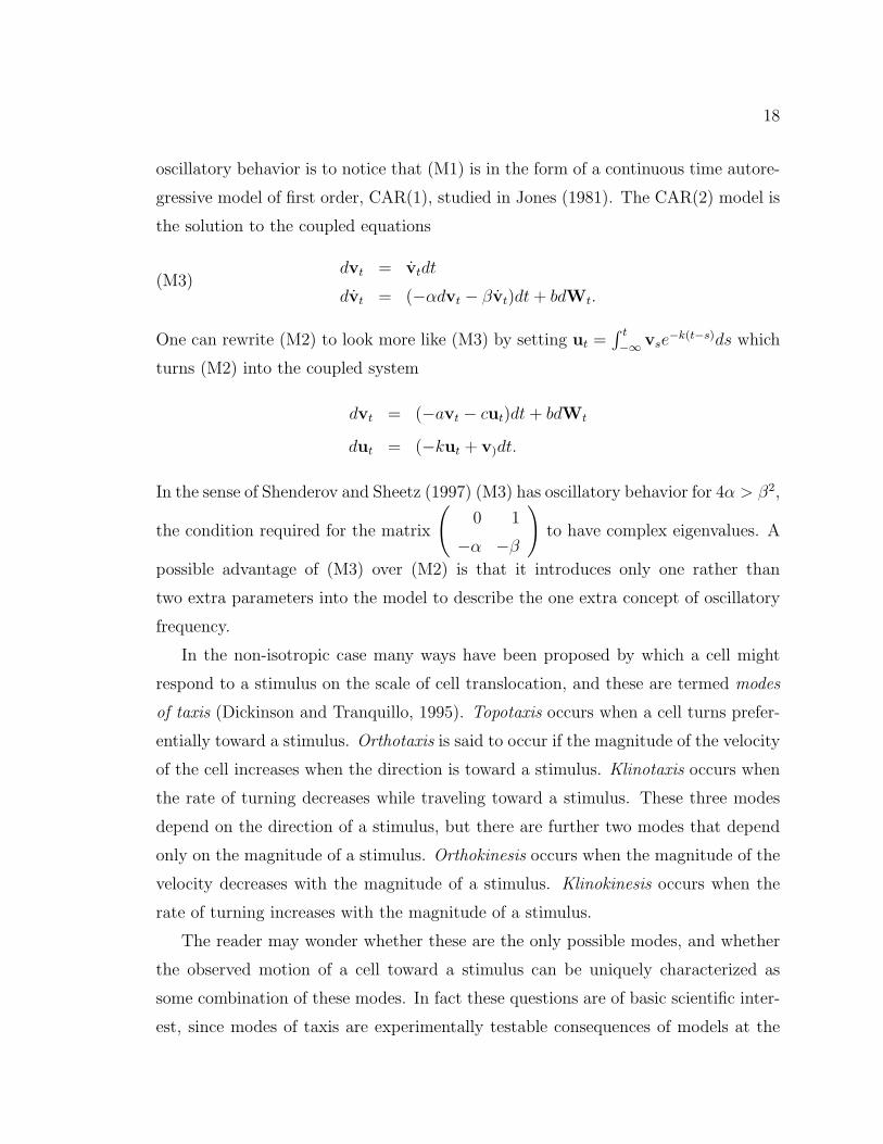
Here (rt, θt) are the polar coordinates for the velocity vt. The coordinate pair

(st, φt) = (st(xt), φt(xt)) gives the magnitude and direction of the stimulus at the

location xt of the cell. For multiple stimuli, st and φt take vector values. W(r)t and

W(θ)t are two independent Brownian motions. Assuming the process (vt,xt) is con-

tinuous, Markov and time homogeneous it is a small restriction to suppose it has a

representation as a solution to (M4) (Karlin and Taylor, 1981). The exact way in

which a solution is found for the infinitesimal equations in (M4) becomes relevant

as the two major competitors—the Ito and Stratonovich solutions—differ when σr,

τr, σθ or τθ are non-constant. For models (M1), (M2) and (M3) the two solutions

20

coincide. Some consequences of the choice of solution will be discussed later.

The coefficients in model (M4) can be given biological interpretations, under some

further assumptions. A reason for writing down the model so generally in the first

place was to make these assumptions explicit. Assuming the cell has no reason to

rotate in a particular direction without a directional cue, (see Alt (1990) for a coun-

terexample), µθ(rt, θt, st, φt) fits the description of a topotaxis term. If µr(rt, θt, st, φt)

can be written as

µr(rt, θt, st, φt) = µ(1)r (rt) + µ(2)

r (rt, st) + µ(3)r (rt, θt, st, φt)

then µ(2)r (rt, st) has the form of an orthokinesis term and µ

(3)r (rt, θt, st, φt) has the

form of an orthotaxis term. Similarly, if σθ(rt, θt, st, φt) can be written as

σθ(rt, θt, st, φt) = σ(1)θ (rt) + σ

(2)θ (rt, st) + σ

(3)θ (rt, θt, st, φt)

then σ(2)θ (rt, st) can stake a claim as a klinokinesis term and σ

(3)θ (rt, θt, st, φt) as a

klinotaxis term. The remaining terms σr, τr and τθ have no clear roles to play in the

existing modes of taxis, indicating that these modes form an incomplete picture of the

possible directional behavior in (M4). For example a change in the random variation

in speed, caused by a varying level of a ligand that interacts with the speed regulation

mechanisms of a cell, might cause directional behavior through a term σr(rt, st).

On the scale of migration when the location xt is supposed to have negligible

memory one can write down an analogue to (M4), namely

(M5) dxt = µ(xt)dt + γ(xt)dWt.

Here γ(xt) is a 2× 2 matrix. Since the stimulus is assumed to depend only on posi-

tion, there is no need to include it explicitly in (M5). In this model the two concepts

of rate of turning depending on position and of speed depending on position are

linked together in the matrix γ(xt). Indeed since the sample paths are not differ-

entiable one has to take a broad minded view about “speed” and “rate of turning”

to recognize γ(xt) as a combined kinesis term for both klinokinesis and orthokinesis.

Similarly µ(xt) can be thought of as a taxis term, combining topotaxis, orthotaxis

and klinotaxis. An alternative interpretation of the parameters in (M5) would come

21

from applying a rescaling argument to (M4). The technique of adiabatic elimination

of fast variables (Gardiner, 1983) can provide such a rescaling for certain particular

cases of (M4).

Choosing between the interpretations of persistence, periodicity, speed and modes

of taxis given by different models requires more precise definitions of these concepts

than are currently available in the biological literature. The goal here has been to

present some options, rather than to come down heavily in favor of any one model.

2.2 Consequences and Applications

Three situations are covered that further develop aspects of the previous section.

A simple version of model (M5) is used to address the question of whether a pure

kinesis is a viable mechanism for directional cell motion, and incidentally to compare

Ito and Stratonovich integrals. Some model free definitions of speed, persistence

and periodicity for cells are suggested. A version of model (M5) is used to quantify

galvanotaxis, the motion of a cell in an electric field, and to justify a model free test.

2.2.1 Do kineses work?

There has been some controversy about whether a cell can move up a gradient of

a ligand (a small signaling molecule) just by adjusting its speed or rate of turning

according to the concentration of the ligand (Doucet and Dunn, 1990). In other

words, do orthokinesis and klinokinesis work as a way of moving up concentration

gradients, or must the cell in fact have some memory or ability to detect gradients. A

careful theoretical study of klinokinesis where the velocity of a bacterium is treated as

a Markov process is undertaken in Stroock (1974). The resulting model fails to give

convincing evidence that kineses can work. The best result obtained there is that if

xt is the R-valued process considered in Stroock (1974), giving the position of the

bacterium up an increasing gradient of a ligand, and f : R→ R is a convex function

then E[f(xt)] is monotone increasing with time. This would also be true if xt were

a random walk, or a martingale.

22

Kinesis may be modeled in a simple but instructive way by considering a stochastic

process xt, taking values in (0,∞), defined by the infinitesimal equation

dxt = σxtdWt. (2.1)

This is a particular case of (M5). The Ito solution is xIt = x0e

Wt−t/2 and the

Stratonovich solution is xSt = x0e

Wt . The reader is referred to Karlin and Taylor

(1981) and Oksendal (1998) for the background on stochastic differential equations

beyond the brief introduction in Section 1.2. Calculating expectations gives

E[xIt | x0] = x0

E[xSt | x0] = x0e

t/2.

So for the Stratonovich solution kinesis works, while for the Ito solution it does not!

There is little scientific reason for preferring one solution to the other, and this result

suggests that there is equally little reason to decide whether a kinesis results in motion

up the gradient or whether there must be an additional taxis for this to occur. It may

be valuable to determine whether speed and rate of turning vary with stimulus level

but an attempt to assign motion up a gradient to this phenomenon has no scientific

basis within the framework of (M5).

2.2.2 Model-based and model-free methods

On many occasions fitting and assessing a model is of direct interest. Examples

of this include generating a model to use for simulation of part of a complex system,

and when a theory to be tested makes explicit claims concerning a particular model.

Fitting models (M1)–(M5) is discussed further in Section 2.4 and Chapter 3. Now we

comment on the other situation where the model itself is secondary to the scientific

question at hand.

Scientists, particularly in the field of biology, are often concerned with comparing

particular experimental groups. Quantities measured to compare these groups do

not necessarily have to make direct substantive sense outside the experiment being

carried out. For example, if cell location is measured every 10 minutes for one hour

23

giving measurements xi, 0 ≤ i ≤ 6 then the mean speed of a cell could be quantified as

S = 16

∑6i=1 |xi−xi−1|. This is a common and not unreasonable measure for comparing

mean speed between experimental groups all observed at 10-minute intervals. With

a sufficiently experienced eye one can compare such a result with results from similar

experiments where it may have been convenient to record at 5- or 15-minute intervals.

A more subtle and serious problem with the statistic S is that it does not always act

as a reliable proxy for the physical concept of mean cell speed. To demonstrate this

suppose that (M1) holds for a pair of control and treatment groups having parameters

(a0, b0) and (a1, b1) respectively. Ifb20a0

=b21a1

but a2 6= a1 then the estimates S0 and

S1 arising from evaluating S for control and treatment groups have ES0 6= ES1. For

model (M1) we can calculate explicitly

E[S] = E∣∣∣∣v0

(1− e−a)

a+ b

∫ 1

0

1

a(1− e−a(1−t))dWt

∣∣∣∣which, after routine algebra, leads to

E[S] =

√πb2

2a

(e−a − 1 + a

a2

). (2.2)

When a is large, so the persistence of the cell is low, we see that for a given value of

b2/a the value of E[S] becomes small.

From this example we see that if one believes model (M1) and yet uses statistic

S then one might be led to conclude that the cell speed varies between treatment

and control when in fact only the persistence varies. To avoid embarrassments of this

kind it is necessary to bear in mind that S is only an observable proxy for a more

objective quantity such as the root mean square velocity

S∗ =

(1

60

∫ 60

0

|vt|2dt

)1/2

.

To check that S is doing its job of substituting for S∗ one could either do further

experiments to find out what happens when S is calculated using smaller time inter-

vals, or fit an appropriate model to estimate what would happen. For example, in

the context of model (M1),

E[(S∗)2] =b2

a. (2.3)

24

If a is constant across an experiment then both S and S∗ scale linearly with b. If not,

the two quantities S and S∗ are less comparable, as can be seen by comparing (2.2)

and (2.3).

2.2.3 A model for galvanotaxis

Recall the experiment described in Example 1 of Section 1.1, where cells are mov-

ing on a microscopic slide in a uniform electric field. The influence of the electric field

on the motion of a cell is termed galvanotaxis. It is of interest to quantify galvanotaxis

to help describe how it varies with experimental treatments. Empirically one notices

that the speed of the cells is not much affected by the electric field (Nishimura et al.,

1996). Theory and observation suggest that changes in cell direction are governed

by local behavior around the edges of the leading Lamella (Dunn et al., 1997). A

model consistent with these considerations as well as the symmetry and translation

invariance of the experiment is (M6), below. This model is an extension of (M1)

and a special case of (M4). The electric field is taken to have magnitude E in the

direction of the positive x-axis, which coincides with the direction θ = 0. The velocity

vt = (vx(t), vy(t))T has polar representation (rt, θt)

(M6) dv =

(−α β sin θt

−β sin θt −α

)vtdt + γdWt

An application of Ito’s lemma shows the polar representation of the infinitesimal

equation defining model (M6) to be

drt =

(−αrt +

2γ2

rt

)dt + γdW r

t

dθt = −β sin θtdt +

(γ

rt

)dW θ

t .

The magnitude of the velocity is governed by the same equation as for model (M1).

The directional behavior of model (M6) is seen to be a rotation of the direction of

motion at rate β sin θt toward θ = 0. Thus (M6) fits the description of a topotaxis.

One could quantify galvanotaxis by fitting (M6), as discussed in Section 2.4, and

using an estimate β of β. Another possibility, attractive for its simplicity, is to

25

calculate an approximation to the so-called score statistic. The likelihood function,

L(α, β), when vt is observed for t in the interval [0, T ] and γ is known, is taken to be

the density of the process (M6) having parameters (α, β, γ) with respect to the process

(M6) with parameters (0, 0, γ), evaluated at vt, t ∈ [0, T ]. This density, which in

formal probabilistic language is termed a Radon-Nikodym derivative, is given by the

Girsanov Theorem (Section 1.2) as

L(α, β) = exp

−β

γ2

∫ T

0

r2t sin θtdθt

− β2

2γ2

∫ T

0

r2t sin2 θtdt− α

γ2

∫ T

0

rtdrt − α2

2γ2

∫ T

0

r2t dt + 2αT

.

The partial derivative of the logarithm of the likelihood with respect to β evaluated

at β = 0 is termed the (Fisher) score statistic for testing the null hypothesis that

β = 0. The score statistic then, up to an unimportant constant factor, is

Z =

∫ T

0

r2t sin θtdθt. (2.4)

In Cartesian coordinates this becomes

Z =

∫ T

0

1

|vt|(vx(t)vy(t)dvy(t)− v2y(t)dvx(t)).

From symmetry considerations, Z has expectation zero when β = 0 (for any value

of α) and so if i.i.d. replicates are available the t statistic can be used to test the

hypothesis that β = 0. This suggests a statistic for a discretely observed process

formed by replacing the integral in (2.4) by a finite sum (Kloeden et al., 1996). When

the locations xt = (xt, yt), t = 0, 1, . . . , T are observed, an approximation to Z is

given by setting xt+1 − xt = rt cos θt, yt+1 − yt = rt sin θt and then constructing the

statistic

Z1 =T−1∑t=1

r2t sin θt(θt+1 − θt).

Biologists currently use the statistic (Nishimura et al., 1996; Fang et al., 1999)

Z2 = (xT − x0)/|xT − x0|.

From symmetry considerations, Z1 and Z2 both have zero expectation whenever the

velocity process has rotationally symmetric distribution, so they can readily be used

26

to test for homogeneity. When the true behavior of the cells is similar to model

(M6), the statistic Z1 gives rise to an approximate score test. The score test is

asymptotically equivalent to a likelihood ratio test (Rao, 1973), and so has similar

asymptotic optimality properties. These statistics are compared in practice as part

of the data analysis in Section 2.3.

2.3 Inference from Cell Tracking Data

For an experiment studying the behavior of isolated cells moving on a microscope

slide, on the scale of translocation, the data consist of M time series each of length

N ,

x(i)j , 1 ≤ i ≤ M, 1 ≤ j ≤ N. (2.5)

Each time series x(i) = x(i)j , 1 ≤ j ≤ N gives the location of a cell in R2, measured

in an appropriate way, at each of N equally spaced time points. Cells that do not

come close enough to a neighbor to interact directly (roughly two cell body diameters)

are presumed to be independent, and, by restricting attention to such cells, the M

time series may be considered independent replicates.

Extensions to this situation include experiments where x(i)j takes values in R3

(Noble, 1990), measurement of additional features beyond cell location (Section 2.5),

dependence between time series, and the case without replications where only one

cell is observed (usually for a longer time).

The location data derive from time lapse microscopy images. An example of

one time frame is given in Figure 2.1. Converting this image data into the form of

equation (2.5) is called the cell tracking problem. One approach to cell tracking is the

manual method of following each cell from frame to frame by eye and making some

visually determined center of the cell as its location. There are existing computer

programs to automate cell tracking (Soll and Wessels, 1998), though none are widely

available or in common use for data sets of the type considered in this thesis. In

practice, an extension of the image processing techniques described in Chapter 4 was

used to produce a satisfactory cell tracking program. An outline of the algorithm is

27

Figure 2.1: One time frame of human keratinocytes moving on a microscope slide,prepared as in Fang et al. (1999) and viewed using differential interference contrastmicroscopy.

as follows.

1. Low frequency components of the image are removed by subtracting off a heavily

smoothed version of the image. This removes only microscopy artifacts, since

the cells are small compared to the size of the image.

2. Thresholding, closing, and filling in connected components are applied, as de-

scribed in Chapter 4, to produce at each time j a group of candidate cell shapes.

Any candidate whose size or length to width ratio is implausible for a cell is

discounted as being an artifact.

3. Each candidate cell at time j is supposed to correspond to the candidate cell

28

at time (j − 1) closest to its position, as long as there is a candidate plausibly

close. Otherwise, the candidate is discounted from the analysis.

4. If two cells at time j − 1 correspond to the same candidate at time j, the two

cells are assumed to have come into contact. They are discounted from the later

analysis, which is intended to be carried out only on single, isolated cells.

5. Each of the M candidate cells at time 1 that has a unique correspondence at

each time j ≤ N gives rise to a time series x(i)j , 1 ≤ i ≤ M, 1 ≤ j ≤ N.

6. An interactive video of the proposed solution to the cell tracking problem is

checked visually, allowing for the correction of mistaken cell identities.

This algorithm, which was implemented in a MATLAB program available from

the author, was sufficient to deal with the two main difficulties of the tracking problem

for the data encountered:

(i) The presence of many features in the image not corresponding to cells. These

could, for example, be artifacts of the microscopy or fragments of organic matter.

Some such features can be noticed in Figure 2.1.

(ii) The tendency of the cells to combine together when they encounter one another

and continue moving slowly as a group.

Two examples of resulting collections of time series are shown in Figure 2.2, for

treatment and control experiments, with and without an electric field, carried out as

described in Example 1 of Section 1.1.

The three models we shall consider here for the unobserved velocity process vt are

(N1) dvt = −αvtdt + σdWt

(N2) dvt =

(−α β sin θt

−β sin θt −α

)vt + σdWt

(N3) dvt = −α(vt − β(1, 0)T ) + σdWt.

29

.......

.... . . . .... . ..

.......

.......

. ......

... . ...

.......

..... .........

.......

.......

0 100 200 300 400 500 600

01

00

20

03

00

40

0

Start pointEnd point

(i)

.......

. ......

.......

.......

.......

.......

.......

0 100 200 300 400 500 600

01

00

20

03

00

40

0

Start pointEnd point

(ii)

Figure 2.2: Cell paths resulting from applying the tracking algorithm to two micro-scope slides. (i) A control experiment, prepared as in Fang et al. (1999), with noelectric field. (ii) A treatment experiment, with an electric field off 100 mV/mm. Thecathode is at the top of the page.

30

(N1) is an Ornstein–Uhlenbeck process. (N2) is the model for galvanotaxis proposed

in Section 2.2 and (N3) is a recentered Ornstein–Uhlenbeck process. (N1) has rota-

tional symmetry above the origin, whereas (N2) and (N3) show directional behavior

for nonzero values of the parameter β. For (N2), β is the rate of rotation toward the

positive x-axis. For (N3), β is the expected velocity in the direction of the positive

x-axis. For each of these models the time series xj, 1 ≤ j ≤ N for a single cell is

modeled by

xj+1 − xj =

∫ j

j−1

vtdt + εj+1 − εj

where εj, 1 ≤ j ≤ N is a sequence of measurement errors which are here taken to

be i.i.d. random variables with distribution N(0, τ 2I). The particular form for the

measurement error does not play a role until Section 2.4.

One interest in deciding whether (N2) or (N3) provides a good description of cell

behavior is that, if one wishes to test whether there is directional behavior, different

models will suggest different test statistics. In Section 2.2, model (N2) was shown to

suggest an approximate score statistic which, written in Cartesian coordinates, takes

the form

T2 =N−1∑i=2

1

|v(i)|(v2y(i)(vx(i + 1)− vx(i))− vx(i)vy(i)(vy(i + 1)− vy(i))).

Here xi = (xi, yi), vx(i) = xi − xi−1 and vy(i) = y1 − yi−1. A similar calculation for

(N3) leads to the statistic

T3 = xN − x1,

th total change in the x-coordinate. One important consideration that may affect the

preferred method of analysis is whether the model is supposed to describe individual or

population behavior. If the model class is parameterized by θ ∈ Θ, one could suppose

that the population is homogeneous, and each individual has the same parameter

θ. If the population is inhomogeneous, with each cell having its own parameter θ′

arising from some distribution on Θ, a parameter such as θ = E(θ′) can be used to

describe the population. For the data considered here, one might suppose that the

directional behavior of all cells is similar, but cells vary in their speed. This might

31

suggest rescaling T3 to give a statistic

T4 =xN − x1

|xN − x1| .

T4 is the same statistic that was introduced under the different name of Z2 in Sec-

tion 2.3, and is the cosine statistic favored in practice by biologists. Based on the

discussion of cell speed in Sections 2.1 and 2.2, a more natural way to scale T3 to

allow for inhomogeneous cell speeds might be

T5 = (xN − x1)

/√√√√ 1

N − 1

N−1∑i=1

|xi+1 − xi|2 .

The t-statistics and corresponding p-values for these four test statistics applied to a

data set collected by Dr. K. Fang are presented in Table 2.1. The treatment group

here consisted of a total of 24 cells prepared on three microscope slides, as previously

described in Example 1 of Section 1.1, and exposed to a direct current electric field

of 100 mV/mm. The 40 control cells were similarly prepared, on four slides, but were

not exposed to the electric field.

treatment group control group t-testsample mean SE sample mean SE p-value

T2 53.5 18.2 29.8 16.3 0.354T3 21.7 5.2 3.6 4.6 0.015T4 0.490 0.126 0.095 0.120 0.035T5 2.21 0.50 0.22 0.49 0.010

Table 2.1: The statistics T2, T3, T4, T5 were calculated for each of the 24 cells in thetreatment group and 40 in the control group. A two sample t-test was carried out totest the hypothesis that the treatment had no effect, against a general alternative hy-pothesis. T2 and T3 have units of pixels (1 pixel ≈ 1µm). T4 and T5 are dimensionlessquantities.

All the test statistics are comfortably positive for the treatment group, indicating

a preference for the cells to move toward the cathode (negative pole) of the electric

field. The statistic T2 has its treatment group average the fewest SE’s from zero, and

also detects possible indications of a similar effect for the control group, leading to a

large p value for the difference between treatment and control.

32

On this data set, the approximate score statistic for model (N3), T3, and is scaled

version, T5, both showed strong statistical evidence for a difference between treatment

and control groups. The cosine statistic, T4, used previously by biologists, gives

slightly weaker evidence. The further exploration of the data set in Section 2.4 will

help to explain these differences.

2.4 Parameter Estimation for Models of Cell

Translocation

Various methods based on moments have been proposed to estimate parameters

for models of cell motion such a model (N1) of Section 2.3 (Dickinson and Tranquillo,

1993; DiMilla et al., 1992). In fact, parameter estimation for (N1) is a well-studied

statistical problem, as it is a linear, Gaussian state space model. Maximum likelihood

estimates are efficient and may be computed using the Kalman filter, as described

in Harvey (1989). Model (N3) is similarly linear and Gaussian. For nonlinear mod-

els, such as (N2), the likelihood may be calculated using sequential Monte Carlo,

as described in Section 1.3. The maximum smoothed likelihood estimator (MSLE)

developed in Chapter 3 provides an effective way to estimate parameters and their un-

certainties from a Monte Carlo likelihood function which had considerable simulation

error even for long computation times. A trick that is available for some Monte Carlo

estimation methods, such as the state space methods of Durbin and Koopman (2000),

is to use the same seed for the random number generator at each parameter value.

When the Monte Carlo likelihood is a continuous function of the parameters for any

fixed sequence of random numbers, this trick allows standard numerical maximization

techniques to be applied. Sequential Monte Carlo, however, uses random numbers for

sequential resampling which leads to a highly discontinuous Monte Carlo likelihood

function even for a fixed sequence of random numbers. For sequential Monte Carlo,

the simulation error must therefore be dealt with directly.

For the following analysis, the observation error parameter was set to τ = 3,

measuring in pixel units (1 pixel ≈ 1µm). This value was based on inspecting the

33

results of the segmentation algorithm, and in particular noticing that the SD of

the location of certain cells which moved little and were presumed to be dead was

around this value. The physical interpretation of τ is as the standard deviation of the

measurement error. However if τ is estimated from the full data it can compensate

for model mis-specification. Large cell displacements, which are rare for the modeled

velocity, may be assigned as large observation errors rather than scientifically relevant

events.

Estimates of the parameters α, σ and β provide a means to quantify persistence,

speed and directionality even when the model is open to question. When the accuracy

of the model is in some doubt, but the parameter estimation is still meaningful, the

error estimates arising from the Fisher information can be misleading. A simple

example is using the sample mean to describe the center of a distribution based on

independent draws from a distribution which is modeled as N(µ, 1) but is in fact

N(µ, σ2) for σ2 6= 1. A solution to this difficulty is to use the form of the error

resulting from thinking of the estimate as the root of an estimating equation (Basawa

et al., 1997). If n i.i.d. observations x1, . . . , xn are made from a distribution on Rd

with density f(x | θ) for θ ∈ Θ ⊂ Rk, giving rise to an MLE of θ, two estimates of

the Fisher information are

I1 =n∑

i=1

(∂

∂θlog f(xi | θ)|θ=θ

∂

∂θlog f(xi | θ)|Tθ=θ

)

I2 = −n∑

i=1

∂2

∂θ∂θTlog f(xi | θ)|θ=θ.

The so-called sandwich estimator of the covariance matrix of θ is

Γ = I−12 I1I

−12 . (2.6)

This estimator is robust to model mis-specification, provided the observations are

independent and the required Taylor series expansion and application of the central

limit theorem of White (1982) are justified. The natural extension of this result from

MLE to MSLE is to replace derivatives of log f(x | θ) by the derivatives of a smooth

approximation to the likelihood. A theoretical justification for this is left as an open

34

problem. For a maximum quadratic likelihood approximation estimator (MQLE),

calculated as below, this error estimate takes an appealing form. Suppose n i.i.d.

random variables are observed, with log likelihoods λi(θ), 1 ≤ i ≤ n giving rise to

a likelihood function

λ(θ) =n∑

i=1

λi(θ).

Let θ be a preliminary estimate of θ and let G ⊂ Θ ⊂ Rk be a grid of points around θ,

as defined and used in Section 3.1 below. Use least squares to fit a quadratic function

to λ(θ∗), θ∗ ∈ G, giving rise to a symmetric matrix Q, a vector b and constant c

such that

λ(θ) ≈ (12)θT Qθ + θT b + c.

If the model possesses LAN, one can hope that Q should be negative definite, in

which case the MQLE, θ, is defined by

θ = −Q−1b. (2.7)

The linearity of least squares fitting gives an identity

b =n∑

i=1

bi,

where bi comes from making a linear fit, using least squares, to λi(θ) − 12n

θT Qθ

evaluated on G, written as

λi(θ)− 1

2nθT Qθ ≈ θT bi + ci.

This suggests an estimated covariance matrix Γ for θ, in terms of the empirical co-

variance, R, of √nbi, 1 ≤ i ≤ n, given by the equation

R =n∑

i=1

bibTi −

1

nbbT (2.8)

Γ = Q−1RQ−1.

This construction of Γ is an extension of the sandwich estimator, given in equa-

tion (2.6), to MQLE. This error estimate can be seen to be robust to model mis-

specification in that it is based on an expression for the covariance that is true for

35

the sum of any i.i.d. random variables (though bi, 1 ≤ i ≤ n are of course only

approximately i.i.d.).

Parameter estimates, with corresponding errors, are presented in Table 2.2 for

the same experimental data discussed in Section 2.3, comparing a treatment group of

human keratinocyte cells exposed to a DC electric field of 100 mV/mm. with a control

group. Model (N1) was only fitted to the control group, as it does not allow for any

rotational asymmetry. Both models (N2) and (N3) have parameter estimates differing

between treatment and control most noticeably in the asymmetry parameter, β. This

supports the belief that the parameters α and σ change little in the presence of an

electric field of 100 mV/min. The error estimates labeled SE1 in Table 2.2 is based on

the Hessian estimator, Q−1, for the variance of the parameter vector θ = (α, β, σ)T ,

coming out of the general theory of maximum likelihood estimation (White, 1982).

SE2 comes from the sandwich estimator Q−1RQ of equation (2.8). SE2 is larger than

SE1 in all cases other than for the estimate of α in model (N1). For the estimates

of β the discrepancies between SE1 and SE2 are not large. The largest discrepancies

occur for estimates of σ, and this may be partially explained by recalling that the

observation noise parameter was fixed for convenience at τ = 3. Assuming that we

know the exact size of the observation noise might be expected to reduce the error

in estimating the innovation noise, σ. SE2, which allows for the possibility of model

mis-specification such as τ 6= 3, and which is constructed in a way similar to the usual

standard error on a mean via the sample variance, is preferred and will be the error

estimate used subsequently.

The estimates of β divided by their SE’s (i.e., in SE units) for models (N2) and

(N3) are similar to the means of the statistics T2 and T3 in SE units. The same

comments therefore apply as in Section 2.3, that the model (N3) discriminates more

strongly between the asymmetry of the treatment and control groups than does (N2).

This may lead one to suspect that the data are better represented by (N3) than by

(N2). There are many formal and informal ways of assessing model fit. Formally, one

can test model specification by comparing the sandwich estimator of the variance of

the parameter estimate with the Hessian estimator (White, 1982). A class of models

may be compared with a larger family of models including the original class (Box

36

treatment controlestimate SE1 SE2 estimate SE1 SE2

N1 α 0.578 0.064 0.060σ 7.15 0.49 0.76

N2 α 0.559 0.097 0.120 0.609 0.066 0.069β 0.455 0.125 0.157 0.212 0.100 0.116σ 7.94 0.66 1.29 7.34 0.50 0.78

N3 α 0.523 0.118 0.177 0.592 0.092 0.130β 4.93 0.93 1.02 0.85 0.71 0.78σ 7.22 0.72 1.39 7.24 0.56 0.93

Table 2.2: Parameter estimates for models (N1), (N2) and (N3) based on a treatmentgroup of 24 cells and control group of 40 cells. The MQLE method of equation (2.7)was used. SE1 corresponds to the Hessian estimator Q−1 and SE2 is the sandwichestimator Q−1RQ of equation (2.8).

and Jenkins, 1970). Estimates, ε(i)j , of the measurement errors, ε(i)

j , are termed

residuals and may be plotted against possible covariates of interest such as time and

the microscope slide label. The clearest evidence found by the author for preferring

model (N3) to (N2) for the data presented in this thesis is a plot of magnitude of

cell displacement against direction, displayed in Figure 2.3. This plot, shown for

the treatment group of cells and for simulations under models (N2) and (N3) with

their fitted parameter values, demonstrates qualitative agreement between the data

and model (N3). In both cases there are relatively few occasions when cells travel

more than 5 pixels in the direction of the anode. Model (N2), however, acquires its

anisotropic behavior just by having fewer occurrences of cells traveling in an anodal

direction. Those cells that travel toward the anode for (N2) do so with almost as large

displacements as those traveling toward the cathode. Observations have been made

in the biological literature that directional factors such as DC electric fields often do

not affect cell speed and persistence (Nishimura, 1996). Here we find that this is

true in the sense that estimates of σ and α are similar for treatment and control, but

not in the alternative sense (which is a property of model (N2)) that the marginal

distribution of cell speed is independent of cell direction.

This section has demonstrated a methodology suitable for fitting a wide class of

37

nonlinear models to cell translocation data. For the two models considered in detail

here, the linear Gaussian model, (N3), appears more satisfactory than the nonlinear

model (N2). However, there are many different types of cells and situations in which

one might be interested in studying their motion. It is reassuring to be able to write

down, fit and assess plausible nonlinear models, even if only to add evidence for the

adequacy of linear ones.

2.5 A Statistical Analysis of Cell Shape

In this section, two models for cell shape are introduced and compared. In each,

the shape is defined by a boundary function in center-radius form. This form was

developed in Section 1.4, together with comments on its strengths and limitations.

First we describe a model based on the principle of local autocatalysis and long range

inhibition for the processes governing the extension of the cell boundary. Secondly

we introduce a model arising from a cytomechanical model based on equations of

fluid dynamics. The forms of these models which appear here are intended to be

phenomenological, meaning that they are simplified caricatures of a complex system.

The system is considered as a “black box”, which one tries to understand by combining

physical insights with observational data. A data analysis is carried out to investigate

the applicability of these models in a practical setting.

A principal that has been widely used to model biological pattern formation, such

as leopard spots and butterfly wings (Murray, 1989), and various other developmental

processes such as exotic sea shell patterns (Oster, 1990) is that an agent acts to

enhance existing features of the process while suppressing the appearance of new

features in some surrounding region. This principal may be applied to cell motion,

by modeling the creation, interaction and dispersion of the protrusions that cells

employ to locomote. In terms of a radial description rt(φ) of cell shape around a

center ct, a model for local autocatalysis and lateral inhibition for a cell moving in

an isotropic environment can be written in terms of at(φ) = log(rt(φ)/r), where r is

38

a characteristic radius of the cell, as

(S1) dat(φ) =

(∫ π

−π

−h(ψ)at(φ + ψ)dψ

)dt + dxt(φ).

Here −π ∈ φ, ψ < π and addition of angles is modulo 2π. The process xt(φ) is

taken to be a Gaussian process, whose increments are stationary in time and whose

distribution is rotationally invariant in φ. It would be of interest to extend (S1) to

anisotropic situations, for example replacing h(ψ) by h(ψ, φ) and/or removing the

rotational invariance requirement on xt(φ), as this would enable a quantification of

the anisotropic behavior. A possible parametric form for h is the difference of two

Gaussian curves, or “Mexican Hat”,

h(φ) = a1f(φ/b1)− a2f(φ/b2) (2.9)

with f(φ) = (1/√

2π)e−φ2/2 and a1 > a2 > 0, b2 > b1 > 0.

A convenient way to study rotationally invariant processes on the circle is through

the Fourier transform. This is discussed in more detail in Section 4.2. We write At(k),

Xt(k) and H(k), k = 0, 1, 2, . . . , for the Fourier transform of at(φ), xt(φ) and h(φ).

Further supposing that Xt(k) can be written as σ(k)Wt(k) for a series of independent

complex valued Brownian motions Wt(k), k = 0, 1, 2, . . . , (S1) becomes

dAt(k) = −H(k)At(k)dt + σ(k)dWt(k). (2.10)

This can be recognized as the infinitesimal equation for a complex valued Ornstein–

Uhlenbeck process.

The frequency domain form of (2.9) is

H(k) = a1b1φ(b1k)− a2b2φ(b2k).

For stability of At(k) we require H(k) > 0 which is satisfied if a1b1 > a2b2. When

the continuous time model (S1) is observed at discrete time points t0, t1, . . . , tN−1,

equally spaced with separation tn−tn−1 = ∆, the evolution equation for the discretely

observed shape function A∆n (k) = Atn(k) is given by

A∆n (k) = e−∆H(k)A∆

n−1(k) +√

(−σ2(k)/2H(k))(1− e−2∆H(k))εn(k), (2.11)

39

where εn(k) are i.i.d. standard normal random variables. The two parameters

defined by H∆(k) = e−∆H(k) and σ∆(k) =√

(−σ2(k)/2H(k))(1− e−2∆H(k)) may be

estimated for each k using standard statistical computing packages, such as S-Plus,

since (2.11) is an AR(1) process.

Another way to arrive at a phenomenological model for cell shape is to take a

simplified form of a cytomechanical model that claims to represent the biophysi-

cal processes involved in cell motion. A stochastic model for receptor-mediated cy-

tomechanics is developed in Tranquillo and Alt (1996). They propose a model for

a(t, φ) = log(r(t, φ)/r) given by the partial differential equation

(S2)∂a

∂t+

1

c1

∂2

∂φ2

(c2

2a + c3ln

(1− a

c4

)+

c5

2

∂2a

∂φ2

)= x(t, φ).

The left-hand side models the physical properties of the cell, using a simplified form

of the two-phase fluid model for the cell cytoplasm of Dembo (1989). The constants

c1, c2, . . . , c5 have interpretations within this model. The right-hand side of (S2) is

supposed to represent receptors on the cell membrane which, when activated, drive

the cell motion process. When the cell is in a homogeneous environment, x(t, φ)

may be modeled by Gaussian white noise. The model (S2) then becomes a stochastic

partial differential equation, as studied in, for example, DaPrato and Zabczyk (1992).

We avoid complications by considering only a linearized form of (S2), which in the

frequency domain representation can be written

dAt(k) = −H(k)At(k) + σdWt(k), (2.12)

where

H(k) = C1k2 + C2k

4

for

C1 =c2

2c1

− c3

c4

, C2 =c5

2c1

.

Here Wt(k) is a collection of independent Brownian motions, indexed by k =

0, 1, 2, . . . . Note that this model specifies that σ is a fixed constant, independent

of k. For stability we require H(k) > 0 for all k, and so C2 > 0, C1 > −C2.

40

Data on the cell shape process are available as a byproduct of the cell tracking

algorithm described in Section 2.3, and some examples are presented in Figure 2.4.

A way to relate these data to (S1) and (S2) is to estimate the coefficients H∆(k) and

σ∆(k) for each k. The Fourier representation of cell shape is used, and compared to

alternatives, in Brosteanu et al. (1997). The models considered here can be thought

of as simple candidates to describe the evolution in time of the Fourier representation

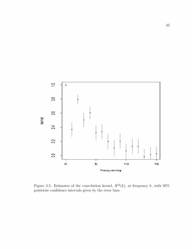
of cell shape. Figures 2.5 and 2.6 show estimates of H∆(k) and σ∆(k) arising from

the data in Figure 2.4. An investigation of the residuals εn(k) suggests only minor

deviation from normality (checked by normal quantile plots such as Figure 2.7) and

little autocorrelation (checked by autocorrelation plots, not shown).

A noticeable feature of the plot of H∆(k) is that it descends down to around zero

for higher frequencies. This corresponds to H(k) becoming large, which qualitatively

favors (S2) over (S1). For (S1), on a scale much smaller than that of h(θ) the shape

process should be only lightly damped. On the other hand, model (S2), in the form

of (2.12) with only three parameters, cannot explain features of the data such as the

high value of H∆(k) at k = 4. Although the models (S1) and (S2) give different, and

complementary, ways to interpret the shape process data presented in Figure 2.4,

neither explains the whole story. The cell shape process and is decomposition into

frequency components remain descriptive statistics, waiting for a parametric form to

accompany them.

41

••

• •

••

• •

•

••

•

•

••

••

•

• •

•

•

•

• ••

•

• ••

••••

•••

•

•

•••

• •

•

• • • •

•• ••

•

••

•

••

•

•

•••

•

•

• • •

•

•

•

•

•

• •

•

••

•••

• •

•

•

•• •

• •

• •

•

•

•

••

•

••

•

••

• •

•

•

•••

•

••

•

•

••

•

•

•

•

•

•

•••

•

•

•

•

•

•

••

•

•

•

• •

••

•

angle (degrees)

dis

pla

ce

me

nt

(pix

els

)

0 100 200 300

05

10

15

20

25

30

(i)

••

•

•

•

•

••

•• ••

•

••

•

••

•

••

•

•

•

•

•

•

•

•

•

•

•• •

•

•

•

•

•

••

•

•

•••

•

•

•

•

••

•

••

•

•

•

••

•

••

•

•

••

•

•

•

•

•

•

•

•

••• •

••

•

•

•

•

•

•

•

•

••

•

•

•

•

•

••

••

•

•

•

•

• •

•

••

•

•

•

•

•

•

•

•

•

•

•

•

•

••

•

•

•

••

•

•

•

••

•

•

•

•

•

•

•

• •

•

angle (degrees)

dis

pla

ce

me

nt

(pix

els

)

0 100 200 300

51

01

52

02

53

0

(ii)

•

•

•

•

•

•

•

•

•

•••

•

•

•

•

•

••

•

•

•

•

•••

•

•

••

•

•

•

••

•

• ••

•• •

•

••

••

• •••

•

•

• •

•

••

•

•

•

•

•

•

••

•

•

•

••

•

•

•

•

••

•

•

•

•

•

••

•

•

•

••

•

•

•

•

•

•

•

•

• ••

••

•

•• •

•

•

••

•

•

••

•

••

••

•

•

••

•

••

•

•

• •

•

•

••

•

•

••

••

•

••

•

angle (degrees)

dis

pla

ce

me

nt

(pix

els

)

0 100 200 300

05

10

15

20

25

(iii)

Figure 2.3: Setting x(i)j+1 − x

(i)j = (r

(i)j cos θ

(i)j , r

(i)j sin θ

(i)j )T , the displacement, r

(i)j , is

plotted against the angle, θ(i)j , for each cell i and each time point j. (i) The treatment

group. (ii) Simulated data for model (N2), using the fitted parameter values. (iii)Simulated data for model (N3), using the fitted parameter values.

42

#1

#2

#3

#4

#5

#6

#7

#8

#9

#10

Figure 2.4: The shapes of ten cells from a control experiment, with no electric field.The cell shapes were recorded at seven equally spaced time points (10 minutes apart),using the algorithm for cell tracking described in Section 2.3.

43

Figure 2.5: Estimates of the convolution kernel, H∆(k), at frequency k, with 95%pointwise confidence intervals given by the error bars.

44

•

•

•

••

• •

••

•• • • • • •

frequency

inno

vatio

n st

anda

rd d

evia

tion

5 10 15

0.0

0.5

1.0

1.5

2.0

2.5

Figure 2.6: Estimates of the innovation standard deviation, σ∆(k), at frequency k.

•

•

••

•

•

••

•

••

••

•

•

•

•

••

•

••

•

•

••

••

••

••

•

•

•

••

•

••

••

••

••

• •

•

• •

•

•

•••

•

•

•

•

•

•

•

•

•

•

•

•

•

•

• •

••••

•

•

•

•

•

•

•

•

•

•

•

•

•

•

•

•

•

•

•

•

•

•

•

•

••

•

•

•

•

•

•

•

••

••

•

•

•

• ••

•

••

•

• •

•

•

•

••

•

•

•

•

•

•

•

•

•

•

••

•

•

•

•

•

•

•

•

•

• •

••

•

•

•

•

••••

•

•

•

•

•

•

•

•

•

•

•

•

•

•

••

•

•

••

•

•

•

•

••• •

•• •

•

•

•

••

•

•

•

••

•

•

•

•

•

•

•

•

•

••

•

•

•

••

•

•

•••

•

•

•

•

••

••

••

•

•

•

• •

•

•

•

•

•

•

•

•

•

•

••

•

••

•

•

•

•

•

•

•

•

••

•

••

•

•

•••

•

•

••

•

•

•

•

•

•

•

• •

•

•

•

•

•

•

••

•

•

•

•

••

•

•

•

•

•

••

•

•

••

••

•

•

•

•

••

•

•

•

•

•

•

•

•

•

•

•

•

•

•

•

•

•

•

• ••

•

••

••

•

••

•

•

•

•

•

•

•

•

•

•

•

•

•

•

••

••

•

•

•

•

•

•

Quantiles of Standard Normal

Res

idua

ls

-3 -2 -1 0 1 2 3

-4-2

02

4

Figure 2.7: A normal quantile plot, for frequency k = 3, of the residual processA∆

n (k)− exp(−∆H(k))A∆n−1(k). Both tails for the residuals are seen to be slightly,

but noticeably, longer than those of the normal distribution. This indicates thatallowance for non-normality might be desirable but would be expected to make littledifference in the estimated quantities.

45

Chapter 3

Asymptotic Theory for Maximum

Smoothed Likelihood Estimation

and an Application to State Space

Models

This chapter develops some asymptotic theory which assists the statistical analysis

of Chapter 2 while making a widely applicable contribution to the general theory of

maximum likelihood estimation and of state space models. The original motivation of

this work was the observation that the best results currently available for the asymp-

totic properties of the maximum likelihood estimator for general non-linear state space

models place heavy restrictions on the form of the model (Bickel et al., 1998; Jensen

and Petersen, 2000). An attractive framework for finding a more widely applicable

result is based on the local asymptotic normality (LAN) property of Le Cam (1986).

Some progress on this project is made in Section 3.2, for a situation where the state

process is a discretely observed diffusion process. A more general result based on the

preservation properties of LAN under information loss (Le Cam and Yang, 1988) is

still an open problem.

The relevance of the LAN framework to applied statistical practice is an important

issue to discuss before embarking on a voyage toward this asymptotic limit. This is

46

a question that has not previously been extensively explored, beyond the comments

in Le Cam (1990), so Section 3.1 takes considerable care to motivate the LAN frame-

work introduced. This is done by showing that the LAN property confers desirable

asymptotic results on a class of estimators resulting from maximizing a smoothed

version of the likelihood in a neighborhood of an effective preliminary estimator.

Maximizing a smoothed version of the likelihood is discussed in Small et al. (2000),

in the context of eliminating multiple root problems for estimating equations. Daniels

(1960) proposed applying a kernel smoother to the likelihood function to aid numerical

evaluation of the maximum. Barnett (1966) found in a simulation study that the

method of Daniels could exceed the efficiency of the maximum likelihood estimator

(MLE) for a Cauchy location model by up to 10%. Kreimer and Rubinstein (1988)

considered smoothing as a general technique for numerical maximization of functions.

Heuristically, there are two main problems that can arise with the maximum like-

lihood estimator but which an LAN based approach avoids. These are demonstrated

in the two examples below.

Example 1 (Normal mixture). A simple situation demonstrating an unbounded

likelihood function is the mixture of two normal distributions of ???. Any mixture

model can be written as state space model, and this is carried out here since state

space models are considered in Section 3.2. The state vector is Xi = (X(1)i , X

(2)i ),

1 ≤ i ≤ n, where X(1)i are i.i.d. N(µ, 1) and X(2)

i are i.i.d. N(µ, σ2) independent

of X(1)i . The observed variables are

Yi =

X

(1)i with probability 1/2

X(2)i with probability 1/2

for µ ∈ (−∞,∞) and σ ∈ (0,∞). Then the likelihood

Ln(µ, σ) =n∏

i=1

(1

2· 1√

2πe−(Yi−µ)2/2 +

1

2· 1√

2πσ2e−(Yi−µ)2/2σ2

)

has an infinite supremum for µ = Y1 and σ → 0.

When fitting such a mixture model, this poor behavior of the MLE can be avoided

by maximizing the likelihood in a region where σ is bounded away from zero. This

47

solution is practical, but theoretically inelegant, and augurs poorly for the existence of

good general results for theoretical properties of the MLE in state space models. On

the other hand, LAN can be shown to hold for Example 1 using Le Cam’s condition

of differentiability in quadratic mean introduced in Section 3.2.

When the likelihood function has many local maxima, the global maximum may

correspond to a narrow spike distant from the main concentration of the likelihood.

This can lead to poor performance of the MLE, and also may make the likelihood

function hard to maximize numerically. Furthermore, error estimates based on the

second derivative of the likelihood at the maximum are then not applicable. One

way to get around these problems is to make a quadratic approximation to the log

likelihood in a neighborhood of the true parameters value in a way that avoids small-

scale features of the likelihood function. One way of doing this is the so called one-

step estimator of Le Cam and Yang (1990). In this thesis, the one-step estimator is

more conveniently called the maximum quadratic likelihood approximation estimator

(MQLE), and is demonstrated in Example 2 for a shift parameter estimation problem.

Example 2 (Many local maxima). The shift family with densities on R given by

f(x | θ) ∝ exp(−|x− θ|α) with respect to Lebesgue measure can be shown to possess

LAN for α > 12

using the criterion of differentiability in quadratic mean discussed in

Section 3.2. For 12

< α ≤ 1 it does not satisfy the Cramer conditions (Cramer, 1946)

for the MLE to attain asymptotically the Cramer–Rao bound. An example of the

likelihood function based on a simulated sample of size 100 with θ = 0 and α = 0.6

is shown in Figure 3.1. The MLE and median are shown, together with the MQLE

calculated by the method employed by Le Cam’s one-step estimator: a quadratic was

fit using the likelihood function values evaluated at the median and points ±0.3 from

the median. This example serves to illustrate the difference between the one-step

estimator and an iteration of Newton–Raphson maximization: the quadratic approx-

imation is carried out on a scale that captures the overall shape of the likelihood,

without being distracted by small-scale behavior. An iteration of Newton–Raphson,

on the other hand, uses a quadratic approximation of a smooth function at an ini-

tial estimate to attempt to approach a local maxima of the function. This gives one

48

−0.25 −0.2 −0.15 −0.1 −0.05 0 0.05 0.1 0.15 0.2 0.25

−158.1

−158

−157.9

−157.8

−157.7

−157.6

−157.5

−157.4

−157.3

−157.2

−157.1

Parameter value, θ

Log−

likel

ihoo

d

MedianMQLE MLE

Figure 3.1: The log-likelihood function for a sample of size 100 drawn from thedensity f(x|θ) ∝ exp(−|x − θ|α) with θ = 0. The median, MLE and MQLE areshown, together with the approximating quadratic.

answer to the question “Why not repeat the one-step estimator twice?” A more con-

vincing explanation of parameter estimation in the LAN framework is given using the

concept of maximum smoothed likelihood in Section 3.1 below.

3.1 Maximum Smoothed Likelihood Estimation

Defining an experiment as a family of probability measures Pθ, θ ∈ Θ, an exten-

sive theory is detailed in Le Cam (1986) for the convergence of experiments to a limit

experiment. An important case is convergence to a Gaussian shift experiment, where

statistical inference for θ becomes asymptotically equivalent to estimating the mean

of a certain Gaussian random variable. A precise treatment of these concepts, which

is not required for reading this thesis, can be found in Le Cam (1986) or Le Cam and

Yang (1990). A widely used example of convergence to a Gaussian shift experiment is

the condition of Local Asymptotic Normality (LAN), defined below. LAN has found

use in many theoretical situations (Bickel et al., 1993; Hallin et al., 1999; Bickel and

49

Ritov, 1996; Hopfner et al. 1990; Jeganathan, 1995). Later in this section conditions

will be found for LAN to hold for the models introduced in Section 2.1. First I am

going to argue for the importance of LAN to applied statistics.

The key to understanding the role of LAN in applied statistics is its close relation-

ship to maximum likelihood estimation (MLE). A difficulty with comparing these two

concepts is that LAN is an asymptotic property of the likelihood function whereas

MLE is a parameter estimation procedure. To level the playing field we must intro-

duce two more acronyms. Write MLAN for the property that the MLE exists, is con-

sistent, and is asymptotically normal, with variance equal to the Cramer–Rao lower

bound. An estimation procedure based on the LAN property, for reasons described

later, will be called maximum smoothed likelihood estimation (MSLE). Clearly, LAN

is most appropriately compared to MLAN and MSLE to MLE.

LAN is a weaker property than MLAN, in the sense that the commonly used

sufficient conditions are weaker. In the case of i.i.d. random variables, the Cramer

conditions for MLAN imply a condition of differentiability in quadratic mean which

in turn implies LAN (Le Cam and Yang, 1990, p. 102). Heuristically, both LAN and

MLAN ensure that the log likelihood ratio in a neighborhood of the true parameter

value θ0 is asymptotically approximately quadratic in θ. MLAN further requires that

the likelihood function be sufficiently smooth and satisfy a global constraint that

the likelihood function should not grow too large for θ distant from θ0. The surprise

about LAN is that it confers similar asymptotic optimality properties on appropriately

constructed estimators, confidence regions and tests to those provided by the stronger

condition MLAN. A discussion with some more details may be found in Le Cam and

Yang (1990, Section 5.8), which builds on a result of Le Cam (1986, Theorem 1

of Section 7.4) that if a sequence of experiments has a Gaussian limit experiment

then one cannot achieve asymptotically risk functions that are not achievable on the

Gaussian limit.

Although we have seen that the local likelihood approximation provided by LAN

has a solid foundation in theory, applications have been restricted by the perceived

lack of a practically justified estimator based on the LAN property. In fact, we are

going to introduce such a maximum smoothed likelihood estimator (MSLE) and show

50

that in many cases it corresponds closely to the method used in practice by responsible

statisticians claiming to be calculating the MLE.

A practical procedure for likelihood-based parameter estimation from a compli-

cated likelihood function might include the following steps

(P1) Take several starting values, θk, 1 ≤ k ≤ K. Hopefully knowledge of the

particular application will suggest some reasonable values of θk. These might

also come from the method of moments, a convenient but usually inefficient

estimation procedure, discussed in Basawa et al. (1997).

(P2) For each θk, run a numerical optimization procedure starting at θk to attempt

to find the maximum of the likelihood function. Hopefully this algorithm will

terminate under a reasonable convergence criterion to give an estimate θk.

(P3) If all the θk are close, use their common value θ for an estimate of θ0. An

estimate of the error on θ can come from numerical calculation of the second

derivative of the likelihood function at θ, using asymptotic properties of the

likelihood function. If and when there are enough data, it may be preferable to

calculate an error estimate in a more data-driven way, such as bootstrap and

jack-knife methods.

(P4) If the values of θk for 1 ≤ k ≤ K vary considerably, try to use knowledge of the

subject matter, the form of the likelihood function and the numerical algorithm

used to understand why. Possibly one or more of the starting values may be

rejected as unreasonable.

(P5) In the event of either (P3) or (P4), it will do no harm to plot the region of interest

of the likelihood function, or to try to find some graphical representation such

as marginal plots if the parameter space is of too high dimension to allow a

standard plot.

If MLAN is proved for some asymptotic limit of the model in question, then the

statistician who follows the above procedure can sleep at night safe in the knowledge

that there is probably not much better that could have been done. He can claim to

51

have approximated the MLE, which has asymptotic optimality properties. It only

remains to check the modeling assumptions and perhaps do some simulations to

investigate the finite sample properties of his estimation algorithm and compare it to

competitors.

The MSLE is defined to be the value of θ maximizing a smooth approximation to

the log likelihood coming from evaluation of the likelihood function on a finite grid,

G, of points which with high probability lie in a neighborhood of θ0 and which are

a subset of a discretization Θ∗ of Θ. Further notation and details follow later. The

MSLE is an extension of the method of centering variables described in Le Cam and

Yang (1990, Section 5.3). The method of centering variables, also called Le Cam’s

one-step estimator, and here the MQLE, attempts to reconstruct from the likelihood

function the approximating quadratic whose existence is asymptotically assured by

LAN. Fitting a second degree polynomial is a special case of smoothing the log-

likelihood, and so MQLE is a special case of MSLE. An auxiliary estimator θ is

required to allow the identification of a grid, G, and a sufficient number of points

from G are used to fit a second degree polynomial with a symmetric quadratic term

(alternatively, the quadratic term may be assumed to take on its known asymptotic

value at θ). The quadratic approximation estimator is the value θ at which this

quadratic is maximized. The theory of Le Cam (1986, Chapter 11) shows that under

LAN the sequence of experiments corresponding to observing θ has the same Gaussian

limit experiment as the original sequence of experiments, which provides asymptotic

optimality properties for θ and associated tests and confidence intervals.

The MSLE is strikingly similar to the method carried out in (P1)–(P5). In par-

ticular, a plot of the likelihood function in a region around the estimated value gives

an approximation to the likelihood function based on evaluations on a grid of points,

as used for the MSLE. The requirement that G take values on a discretization Θ∗

prevents evaluation of the likelihood function at particular points where it might be

badly behaved. Such a discretization will be unimportant if the likelihood is smooth,

but if not it provides a useful trick to avoid evaluating the likelihood at particular

points where the likelihood may have peculiarities (for example, the median or an

MLE of a location parameter for a density with a singularity).

52

The similarity between MSLE and good practice is strong enough that MSLE

theory can help support practice. Although people who have tried to use numerical

methods to maximize a likelihood know how important the initial values can be, hav-

ing the requirement of a good auxiliary estimator cast into the theory suggests that

more time should be spent justifying initial values than, say, arguing for the smooth-

ness of the likelihood function which turns out to be unnecessary, if a discretization

trick is used.

Another major reason to prefer the LAN/MSLE theory to MLAN/MLE is that

in many situations MLAN does not hold. A humorous account of things that can go

wrong with MLE is given in Le Cam (1990). The well-known sufficient conditions for

MLAN are restrictive, and not easy to check for complicated likelihood functions. In

fact it is quite possible that the statistician employing (P1)–(P5) slept soundly not

because he had proven that MLAN holds in his model, but because MLE is a principle

which is frequently justified, in a somewhat circular argument, by its widespread use.

However, since the method (P1)–(P5) more closely resembles MSLE, the statistician’s

application of MLE could in fact be marked up as another successful use of MSLE.

Finally, suppose that our statistician has a theoretical bent, and manages to show

that MLAN does indeed hold for his model. He could have saved himself time and

effort by checking the weaker condition of LAN instead. For an example of this,

compare the two papers Bickel and Ritov (1996) and Bickel, Ritov and Ryden (1998),

in which conditions are found for hidden Markov models to have LAN and MLAN

respectively. Another example of LAN being considerably more convenient to work

with than MLAN, that will play a role in this thesis, is the preservation of LAN under

information loss in quite general situations (Le Cam and Yang, 1988). No such results

appear to exist for MLAN.

The time has come to formalize some of the concepts introduced above. A family

Pθ, θ ∈ Θ of probability measures on (Ω,F) indexed by a set Θ forms an experiment

in the sense of Le Cam (1986, Chapter 1). Following Le Cam and Yang (1990,

Chapter 5) we shall take Θ to be an open subset of a fixed Euclidean space Rd,

and limit ourselves to indicating possible generalizations. The quantitydPφ

dPθ, φ ∈ Θ,

denotes the Radon–Nikodym derivative of the absolutely continuous part of Pφ with

53

respect to Pθ. Now let Pθ,n, θ ∈ Θ be a family of measures on (Ωn,Fn) for each

integer n > 0, and define the log likelihood ratio

Λn(φ, θ) = logdPφ,n

dPθ,n

.

To simplify notation we use the op convention. For a sequence ξn of random vari-

ables and a real sequence αn, write ξn ∼ op(αn; θ) if ξn/αn → 0 in Pθ,n measure,

i.e., for any ε > 0, limn→∞ Pθ,n|ξn/αn| > ε = 0. Conventionally, one also abuses the

notation by writing ξn = op(αn; θ).

Definition. The family Pθ,n, θ ∈ Θ has local asymptotic normality (LAN) at θ0 if

there exists a positive definite matrix K and a sequence of random variables ∆ntermed centering variables, such that for any bounded sequence tn ∈ Rd

(i) Λn

(θ0 +

tn√n

, θ0

)= tTnK1/2∆n − 1

2tTnKtn + op(1; θ0)

(ii) ∆nd→ N(0, I) under Pθ0,n.

Slight variations on the definition of LAN are used, with different tradeoffs be-

tween simplicity and generality, in Basawa and Prakasa Rao (1980), Ibragimov and

Has’minski (1981), Le Cam (1986, Section 11.7) and Le Cam and Yang (1990). One

can consider rates of convergence other than√

n, or allow for random matrices Kn

(the local asymptotic quadratic condition of Le Cam and Yang (1990)).

We proceed to construct an MSLE and show that it has the same asymptotic

properties as the method of centering variables, while having more finite sample

justification. Let Θ∗n = 1√

nZd be a discretization of Θ for each integer n. For some

√n-consistent estimator θ, let θ∗ = argminθ∗∈Θ∗n |θ − θ∗| and define a grid Gn to be

the set

Gn = θ∗n +1√n−M,−M + 1, . . . , M − 1,Md

for some integer M > 0. The fixed integer M can be chosen so that the grid Gn ⊂ Θ∗n

surrounds the true parameter value θ0 with high probability. For any ε > 0, we

assume that M and n0 can be chosen so that Pθ0,n

|θ∗n − θ0| < M

√d√

n

< ε for all

54

n > n0. This follows from, or can be taken as a definition of, the√

n-consistency of

θn.

A smoother, S, takes a function on a grid G ⊂ Rd to functions on Rd. Let

G = −M,−M +1, . . . , M −1,Md and define an arbitrary function g : G → R with

t∗ 7→ g(t∗). Suppose S has the following properties, for each t ∈ Rd and any fixed g:

(S1) s(t) = S(g)(t) is continuously differentiable.

(S2) If q is a second degree polynomial on Rd with symmetric quadratic part, there

is a constant C such that for g(t∗) = q(t∗) + ε(t∗),∣∣∣∣dS

dt− dq

dt

∣∣∣∣ < maxt∗∈G

ε(t∗) · C(1 + |t|).

Property (S2) formalizes a requirement that if g(t∗) can be interpolated approx-

imately by a second degree polynomial q(t) then the smoother produces a function

S(g) close to q. A trick that may modify a smoother S ′ (such as the loess program in

the package S-plus described in Venables and Ripley (1995)) to satisfy (S2) is first to

choose 1/2(d+1)(d+2) distinct points of G and interpolate them by a second degree

polynomial q∗ with symmetric quadratic part. Then let

S ′′(g) = q∗(r) + S ′(g(t∗)− q∗(t∗)),

where q∗(t∗) is a mildly abusive abbreviation for the restriction of q∗ to G. The

modification S ′′ of S ′ will satisfy (S2) as long as S ′ takes small functions on G to

small, smooth functions on Θ which one would expect of any reasonable smoother.

The particular function we are interested in finding a smooth approximation to is

the rescaled log likelihood

λn(t) = Λn

(θ∗n +

t√n

, θ∗n

).

Evaluating λn(t∗) on t∗ ∈ G is equivalent to evaluating Λn(θ∗, θ∗n) on θ∗ ∈ Gn. Now

set

t = argmaxt∗∈G

S(λn(t∗))

55

and define the MSLE by

θn = θ∗n +t√n

.

Lemma 3.1 Suppose Pθ,n has LAN at θ0 with matrix K and centering variables

∆n. Let Qθ,n be the law under Pθ,n of an Rd-valued random variable Tn. If |Tn −∆n| = op(1; θ0) then Qθ,n also has LAN at θ0 with matrix K.

Proof. The lemma is a special case of Theorem 4 of Le Cam and Yang (1988). ¤This result says heuristically that if |Tn−∆n| becomes small then Tn is an asymp-

totically sufficient statistic for θ. The proof is based on formalizing this idea of

asymptotic sufficiency. A sequence Tn of statistics is called distinguished if there is

no asymptotic information loss from observing the statistic Tn rather than the out-

come of the experiment Pθ,n. A formal definition of distinguished statistics and some

powerful properties are given in Le Cam (1986, Section 7.3). Perhaps a surprising

feature of Lemma 3.1 is that Tn approximating ∆n under Pθ0,n is enough to show thatdQθ,n

dQθ0,napproximates

dPθ,n

dPθ0,nfor θ in a neighborhood of θ0.

Theorem 3.1 Let Qθ,n be the law of the MSLE, θn, under Pθ,n. If Pθ,n has LAN

at θ0 with matrix K, then Qθ,n also has LAN at θ0 with the same matrix K.

Proof. Writing Tn =√

nK1/2(θn − θ0) and letting ∆n be a centering variable for

Pθ,n, in order to apply Lemma 3.1 it is enough to show that |Tn −∆n| = op(1; θ0).

Let qn(t) = tT K1/2∆n − 1/2tT Kt be the quadratic identified in the definition of

LAN for Pθ,n. As G is finite, from LAN we have

maxt?∈G

(λn(t∗)− qn(t∗)) = op(1; θ0).

The maximum of qn(t) occurs attn = K−1/2∆n. Set Sn(t) = S(λn(t∗))(t), with a

maximum at θn

∣∣∣∣d

dtSn(t−

tn)

∣∣∣∣ >

∣∣∣∣d

dtqn(t−

tn)

∣∣∣∣−∣∣∣∣d

dtSn(t−

tn)− d

dtqn(t−

tn)

∣∣∣∣ .

56

The first term on the right grows linearly in t, and the second term grows as (1 +

|t|)op(1; θ0) by (S2). Thus for ε > 0,

limn→∞

Pθ0,n

(inf

|t−tn|>ε

∣∣∣∣d

dtSn(t−

tn)

∣∣∣∣ > 0

)= 1.

From (S1), any maximum of Sn(t) must have ddt

Sn(t) = 0, giving |tn −tn| = op(1; θ0)

and hence |Tn −∆n| = op(1; θ0). ¤

An alternative approach to demonstrating asymptotic properties of an MSLE,

θn, is to notice that it is asymptotically close to Le Cam’s quadratic approxima-

tion estimator, which we denote as θn. The quadratic approximation estimator is a

particular example of an MSLE, so the argument used to prove Theorem 3.1 shows

that |θn − θn| = op(1/√

n; θ0). The estimator θn thus inherits from θn the properties

demonstrated in Le Cam and Yang (1990) of being consistent and asymptotically

normal with large n asymptotic variance (nK)−1. One can either use the theoretical

value of K, if it is known, or find an estimate Kn. Such an estimate is found and

used in the extension of the quadratic approximation estimator to the case of random

matrices Kn described in Le Cam and Yang (1990, Chapter 5). Under the additional

assumptions (S3) and (S4) below on the smoother, S, the second derivative matrix

at θn can be used to estimate K.

(S3) S(t) = S(g)(t) is twice continuously differentiable.

(S4) If q is a linear-quadratic function on Rd, with symmetric quadratic part, there

is a constant C such that for g(t∗) = q(t∗)+ ε(t∗) and ‖ ·‖ the matrix supremum

norm ∥∥∥∥d2s

dt2− d2q

dt2

∥∥∥∥ ≤ maxG

ε(t∗)C.

Taking q(t) as the linear-quadratic function appearing in the LAN condition, as in

the proof of Theorem 3.1, (S4) allows d2sdt2

evaluated at any point and therefore at θn

to be used as an estimator Kn with |K − Kn| = op(1; θ0), using the supremum norm

for matrices given by |A| = supi,j |Aij|. The condition (S4) looks like a derivative of

57

(S2). When (S2) and (S3) hold, it is therefore not much more to ask that (S4) hold

also.

A generalization of LAN, replacing K by random matrices Kn and requiring that

∆n conditional on Kn is asymptotically normal, is called local asymptotic mixed

normality (LAMN). Many results for LAN can be extended to LAMN, which occurs

naturally in the study of certain non-stationary processes such as branching processes

(Jeganathan, 1995). Under an additional contiguity requirement the quadratic ap-

proximation estimator keeps many of its asymptotic properties under LAMN (Le Cam

and Yang, 1990, Chapter 5), and one might expect the MSLE to do likewise.

Another possible extension would be to relax the requirement for LAN that Θ is

an open subset of Rd. Allowing for θ0 to take values on the boundary of Θ is useful for

hypothesis testing but rather less so for the parameter estimation problem developed

here. Many of the complexities arising from an inability to approach θ0 from all

directions are dealt with in Le Cam (1986). The definition of LAN extends readily to

more general spaces than Rd equipped with an inner product and a quadratic form K.

The quadratic approximation estimator however makes use of the ability to span Θ

using a finite subset. LAN has been used effectively for non-parametric problems with

Θ an infinite dimensional space (Bickel et al., 1993), though our focus on parametric

problems solved by methods similar to (P1)–(P5) does not lead us in that direction.

Last in this list of issues, for which the reader is directed elsewhere for details, is the

use of Theorem 3.1 to make asymptotic optimality claims concerning θn. The matrix

K is thought of as the information about θ in the experiment, and coincides with the

Fisher information under regularity conditions (Le Cam, 1986, Chapter 17.3). One

might say that θn contains asymptotically all the information about θ in Pθ,n. To

formalize this we state a result analogous to an asymptotic form of the Cramer–Rao

lower bound, called Hajek’s convolution theorem and given in this form in Le Cam

and Yang (1990, Section 5.6).

Theorem 3.2 Suppose Pθ,n is LAN at θ. For the experiments Et,n = Pθ+t/√

n,n, t ∈Rd let Tn be an estimate of At for a given non-random matrix A. Assume that

Tn−At tends in distribution under Pθ+t/√

n,n to some random vector H whose distri-

58

bution does not depend on t. Then H shares its distribution with AK−1/2Z +U where

Z is N(0, 1) independent of a random vector U .

The property that U = 0, enjoyed by θn and therefore also θn, might reasonably be

called asymptotic efficiency, a term usually reserved for asymptotically achieving the

Cramer–Rao bound. Clearly Theorem 3.2 implies a variance bound which coincides

with the Cramer–Rao bound when MLAN holds. The usual statement of the Cramer–

Rao bond requires an estimator to be unbiased, though there are extensions for biased

estimators (Casella and Berger, 1990, Section 7.3). The condition for the convolution

theorem analogous to asymptotic unbiasedness is that the estimator Tn is assumed

to have an asymptotic shift invariance property, as the distribution of H does not

depend on t.

3.2 Checking LAN for State Space Models

A useful way to check that LAN holds is through a condition, introduced in

Le Cam (1986), called differentiability in quadratic mean (DQM). After discussing

DQM a version of DQM for conditional experiments will be introduced and used

to show that LAN holds for the models in Section 2.1. DQM is a property of a

single experiment Pθ, θ ∈ Θ and in this setting Pθ,n is the product experiment of n

independent versions of Pθ. Here, as before, θ takes values in an open subset Θ of Rd.

We are now making an independence requirement, that Pθ,n be a product measure,

which was not assumed in Section 3.1.

Definition. A family of probability measures Pθ, θ ∈ Θ is said to be differentiable

in quadratic mean (DQM) at θ0 with derivative V if E[|V |2] < ∞ and

(i) limθ→θ0

1

|θ − θ0|2E[√

dPθ

dPθ0

− 1− (θ − θ0)T V

]2

= 0

(ii) For β(θ, θ0) the mass of the Pθ0 singular part of Pθ,

limθ→θ0

1

|θ − θ0|2β(θ, θ0) = 0.

59

DQM (ii) is a contiguity condition, a form of asymptotic absolute continuity of mea-

sures, which is required to make the following result hold. Theorem 3.3 shows that

DQM implies LAN, and gives a partial converse result.

Theorem 3.3 (Le Cam, 1986) If Pθ is DQM at θ0 with derivative V then the

product experiment Pθ,n has LAN at θ0 with K = E[V V T ]. A converse holds, that

if Pθ,n has LAN at θ0 and ∆n can be written as

∆n =1√n

n∑

k=1

Xk

for Xk i.i.d. copies of a random vector X, then Pθ is DQM at θ0.

In multivariate situations, checking that DQM holds can be awkward (Le Cam and

Yang, 1990, Section 6.3). In this section, we introduce a conditional form of DQM and

show how it forms a convenient tool for checking DQM in multivariate situations with

a natural conditional structure. Let PX,Y (θ) be a family of joint distributions for

random variables X and Y . Assuming regular conditional probabilities exist (Durrett,

1991, p. 198) they can be used to define a conditional experiment PY |X(θ) where

Y takes on its distribution conditional on the outcome of the random variable X.

Definition. PY |X(θ) is conditionally DQM given X at θ0 with derivative W if

E[W 2] < ∞ and

(i) limθ→θ0

1

|θ − θ0|2E[√

dPY |X(θ)

dPY |X(θ0)− 1− (θ − θ0)

T W

]2

= 0

(ii) For γ(θ, θ0, X) the mass of the PY |X(θ0) singular part of PY |X(θ),

limθ→θ0

1

|θ − θ0|2E[γ(θ, θ0, X)] = 0.

The following proposition shows how DQM follows in a bivariate situation where

DQM can be shown for one variable and conditionally for the other. A proof is left

to Appendix A.

60

Proposition 3.1 If PX(θ) is DQM at θ0 with derivative V and PY |X(θ) is con-

ditionally DQM at θ0 with derivative W then PX,Y (θ) is DQM at θ0 with derivative

V + W .

When Pθ is the law of a time series Yj, 1 ≤ j ≤ N, as for the models proposed

in Section 2.1 for cell tracking data, Proposition 3.1 allows us to check the DQM

condition by showing that DQM holds for Y1 and Yj | Y1, . . . , Yj−1 for 2 ≤ j ≤ N .

A property of DQM that will become useful is the preservation of DQM under

information loss. Proposition 3.2 is a statement to this effect taken from Le Cam and

Yang (1988, Section 7).

Proposition 3.2 (Le Cam and Yang, 1988) Let Pθ, θ ∈ Θ be a family of mea-

sures on a sigma algebra A and let Qθ be the restriction of Pθ to a sigma algebra

B ⊂ A. If Pθ satisfies DQM at θ0 then so does Qθ.

A final general result concerning DQM gives sufficient conditions for DQM in

terms of the Fisher information, when the required derivatives exist.

Proposition 3.3 Suppose that for θ ∈ Θ ⊂ Rd, Pθ has a density p(x, θ) with respect

to a dominating measure ν. Suppose further that

(i) p(x, θ) is continuously differentiable in θ for ν almost all x with derivative pθ(θ).

(ii) s(θ) = pθ(θ)p(θ)

1p(θ)>0 satisfies |s(θ)| ∈ L2(Pθ).

(iii) The Fisher information defined by

I(θ) =

∫s(θ)sT (θ)dPθ

is a continuous function of θ.

Then Pθ satisfies DQM with derivative s(θ).

Proof. This result is Proposition 2.1.1 of Bickel et al. (1993) combined with their

statement on page 15 on the equivalence between DQM and their definition of a

regular parametric model.

61

Application of Proposition 3.2 to a state space model setting shows that often one

need check DQM only for the state process to guarantee DQM for the observation

process. This requires that the observation process be a non-random function of

the state process and that the function should not depend on the parameter θ. An

example occurs when vt is velocity, xt = x0 +∫ t

0vtdt is position for t ≥ 0 and (vt, xt)

forms a Markov process. A discrete time state space model is defined for n = 1, . . . , N

by

(L1)Xn = (vn, xn, εn)

Yn = xn + εn

for independent random vectors εn which might represent measurement error.

When (vt, xt) is a continuous process defined as the solution to an infinitesimal

equation such as those in models (M1)–(M4), one is led to look for sufficient condi-

tions for (v1, x1) to satisfy DQM conditional on (v0, x0). We demonstrate in Propo-

sition 3.4 a set of conditions (D1)–(D5) below. These conditions are designed to

include the Ornstein–Uhlenbeck process (model (M1)) when the diffusion coefficients

are smoothly parameterized by θ ∈ Θ, and other similar though not necessarily linear

diffusions. The requirement made that the log transition densities have quadratic

tails is very restrictive though it does cover many cases of practical interest. The

method of proof for Proposition 3.4 could be applied to other situations, but we were

unable to construct a simple and more general statement. Thus conditions (D1)–(D5)

are best thought of as one example for which the method of proof in Proposition 3.4

can be used.

There is a reasonably large literature on statistical inference for discretely observed

diffusion processes, though we are not aware of previous results similar to Proposi-

tion 3.4 below. Dacunha–Castelle and Florens–Zmirou (1986) give asymptotic results

when the discretization intervals tend to zero. Bibby and Sorensen (1995) use mar-

tingale estimating functions and obtain asymptotic results with the discretization

interval fixed. Jensen and Pedersen (2000) look at diffusions that can be written as

transformations of a linear diffusion, which when observed discretely become the well

studied AR process.

62

We consider a family of diffusion processes in Rd parameterized by θ ∈ Θ, an open

subset of Rk, satisfying the infinitesimal equations

dXt = µ(Xt, θ)dt + γ(Xt, θ)dWt.

Here Wt is a standard Brownian section in Rd, γ = γ(Xt, θ) is a d × d matrix, and

we set Γ(Xt, θ) = γγT . Let PX1|X0(θ) be the conditional law of X1 given X0, and let

p(ϕ, x, t) be the density of Xt at x when X0 is distributed with a density ϕ. In this

notation the dependence of p on θ is suppressed, x takes values in Rd, t lies in the

interval [0, 1] and ϕ is a fixed probability density.

(D1) µ and Γ have uniformly continuous partial derivatives µθ, µx, µθx, Γθθ, Γxx, Γθxx

with respect to x and θ. Subscripts are used here to denote vectors and higher

dimensional arrays of partial derivatives, so µx =(

∂µ∂x1

, . . . , ∂µ∂xd

)T

.

(D2) p(ϕ, x, t) has continuous first and second partial derivatives px and pxx, and

there exist symmetric positive definite matrices A = A(θ), B = B(θ) and

positive scalars a = a(θ), b = b(θ) such that for 0 ≤ t ≤ 1 and x ∈ Rd

ae−xT Ax < p(ϕ, x, t) < be−xT Bx

be−xT Ax >

∣∣∣∣∣∑

i

∂

∂xi

(µθp)− 1

2

∑ij

∂2

∂xi∂xj

(Γθp)

∣∣∣∣∣

(D3) For any function η in L1(Rd) with |η(x)| ≤ be−xT Bx, there is a scalar c = c(θ)

such that for 0 ≤ t ≤ 1

|p(η, x, t)| ≤ ce−xT Bx

where p(η, x, t) is defined for η in L1(Rd) by linear extension from η in the set

of probability densities η : η(x) ≥ 0,∫

ηdx = 1.

(D4) a(θ), b(θ), c(θ), A(θ), B(θ) are continuous functions of θ.

(D5) 2B(θ)− A(θ) is positive definite for all θ ∈ Θ.

63

Example. Let Xt be an Ornstein–Uhlenbeck process in R1 with infinitesimal equa-

tion

dXt = θ1Xtdt + (θ2)1/2dWt

and X0 ∼ N [µ0, σ20]. Let A = (inf0≤t≤1 var(Xt))

−1, B∗ =(sup0≤t≤1 var(Xt)

)−1and

Θ = (θ1, θ2) : 2B∗−A > 0. (D1) clearly holds, and since the marginal distributions

are all Normal one can readily see that (D2)–(D5) hold for θ ∈ Θ with A as above

and B = B∗ − ε for any ε > 0.

Proposition 3.4 Suppose PX1|X0(θ) and the density ϕ of X0 satisfy conditions (D1)–

(D5) at θ0. Then PX1|X0 satisfies DQM at θ0.

Proof. The density p(ϕ, x, t) of Xt satisfies the forward equation for t > 0 (Karlin

and Taylor, 1981)∂p

∂t− Lp = 0 (3.1)

with L =∑

i∂

∂xiµ − 1

2

∑ij

∂∂xi∂xj

Γ and initial condition p(ϕ, x, 0) = ϕ(x). Following

Stroock (personal communication) we note that, if it exists, the partial derivative

with respect to θ, denoted with a subscript, satisfies an equation derived from (3.1)

∂pθ

∂t− Lpθ = Lθp (3.2)

with Lθ =∑

i∂

∂xiµθ− 1

2

∑ij

∂2

∂xi∂xjΓθ and initial condition pθ(ϕ, x, 0) = 0. The forward

equation fell out of fashion for probabilistic applications because of difficulties with

existence and particularly uniqueness of solutions. In this setting, (D1)–(D2) are

strong enough to apply general results for parabolic equations, such as Lieberman

(1996, Theorem 5.15), to give the existence of a unique solution to (3.1) and (3.2).

Denoting the right-hand side of (3.2) as f(x, t) the solution to (3.2) can be written

in terms of the solution to (3.1) using the linearity of L,

pθ(ϕ, x, t) =

∫ t

0

p(f(·, s), x, t− s)ds.

Condition (D2) gives f(x, t) < be−xT Bx and then (D3) gives

|pθ(ϕ, x, t)| < ce−xT Bx. (3.3)

64

We now proceed to verify the three requirements needed to apply Proposition 3.3,

writing p(x, θ) for p(ϕ, x, 1).

(i) The continuity of pθ(x, θ) as a function of θ can be seen to hold under (D1)

by considering a diffusion (Xt, θ) on Rd × Θ. The θ component is a trivial

diffusion—it remains constant—but one can still write down analogous equa-

tions to (3.1) and (3.2). Uniform continuity of Lθp as a function of θ and then of

pθ as a function of θ then comes from applying the Holder continuity bounds of

Lieberman (1996, Theorem 5.15) to the initial conditions of (3.1) and the right-

hand side of (3.2) respectively. This trick was suggested by Stoock (personal

communication).

(ii) The inequality (3.3) together with conditions (D2) and (D5) show that the score

function s(θ) = pθ(x, θ)/p(x, θ) is in L2(p(x, θ)), as

|s(θ)| < (c2/a) exp−xT (2B − A)x.

(iii) The Fisher information is

I(θ) =

∫(pθ(x, θ))2

p(x, θ)dx.

From part (i), the integrand converges pointwise in θ for almost all x. Using (D4),

the bound from part (ii) provides a uniform bound in a neighborhood of θ (recall that

Θ is open) and so by dominated convergence the integral I(θ) is continuous in θ. ¤

3.3 Concluding Remarks

This chapter has discussed some implications for statistical practice of asymptotic

theory built around the property of local asymptotic normality (LAN). This property

was used to justify a parameter estimation procedure involving maximization of a

smooth approximation to the likelihood function (MSLE), and also to give error

estimates for this procedure. The asymptotic results place only weak restrictions

on the particular smoothing method used. In practice one has to choose a particular

65

method, and often a bandwidth parameter to go along with it. A number of methods,

including simulation and bootstrap techniques, are available to address these issues

(Silverman, 1985).

Section 3.2 developed some results to show how the state space models proposed in

Section 2.4 fit into the framework of Section 3.1. State space models have been found

useful in many applications, some of which were discussed in Section 1.4. In addition,

mixture models can be written in state space form (Example 1, this chapter), as can

many methods for nonparametric regression (Wood and Kohn, 1998). The method of

MSLE is not however limited to state space models, and might assist in the analysis

of many parametric models where the likelihood function is either not smooth or

can only be estimated using Monte Carlo simulation. Another situation where these

conditions arise is spatial statistics, which involves modeling using random fields

(Cressie, 1993).

Estimators not based on the likelihood function are sometimes prefered in practice

when evaluating and maximizing the likelihood function is found to be difficult. Ex-

amples include the use of moment estimators for cell motion parameters (Dickinson

and Tranquillo, 1993b; DiMilla et al., 1992), the use of various forms of pseudo-

likelihood for random field models (Besag, 1974), and the use of estimating equations

for regression analysis of longitudinal data (Liang and Zeger, 1986). Likelihood based

methods, such as MLE and MSLE, have a major advantage that they can be shown

to be asymptotically efficient in many situations. It is at least reassuring to be able

to compute an estimator that can be shown to be efficient, even if it does not become

the method of choice (for example, if the extra computational labor is found not to

yield much improvement in the estimator). The MSLE introduced in this chapter,

by being both more generally applicable and possibly more readily computable than

the MLE, may facilitate likelihood based analysis.

66

Chapter 4

A Statistical Analysis of Data

Arising from Staining Fixed Cells

Fixing and staining cells or tissues is a standard procedure which involves adding a

preservative chemical followed by an observable marker that can be used to determine

where a particular molecule concentrates in a cell or collection of cells (Lodish et al.,

1995, Chapter 5). In the study of cell motion such experiments can complement time

lapse video microscopy of living cells (Fang et al., 1999). This chapter correspondingly

complements our Chapters 2 and 3 by considering some statistical issues arising from

the analysis of digitized images of fixed, stained cells.

In the experiment motivating this chapter and reported in Fang et al. (1999),

scientists were concerned whether a protein stained for using a monoclonal antibody

is implicated in the mechanism that a cell uses to direct its motion toward a stimulus.

Human skin cells were placed on a microscope slide and an electric field applied,

as described in Section 1.2. After a certain time interval the cells were fixed with

paraformaldehyde, stained and captured as a digital image. An example of a typical

observation is shown in Figure 4.1. The stain was expected to attach preferentially

to the cell membrane, and indeed a boundary region of high stain intensity was

seen. A traditional way to statistically compare the images from different treatment

groups is for an observer to estimate some quantity relevant to the hypothesis in

question. In our example a cell might be given a score of “1” if the boundary staining

67

Figure 4.1: A cell from the treatment group. The electric field is oriented with thecathode at the top of the page.

appears concentrated toward the cathode, and “0” if it appears concentrated toward

the anode. This technique, termed manual scoring, can be time consuming, simplistic

and difficult to make objective. Unless care is taken to ensure the observer is unaware

of the treatment group, a procedure termed blinding, unintended observer bias can

have important consequences (Freedman et al., 1998). A goal of this chapter is

to present a more formal and impartial analysis which produces more informative

summaries of experimental results and efficient tests of relevant hypotheses.

Section 4.1 introduces an algorithm that has been successfully implemented in a

computer program to estimate the boundary of a cell and the intensity of the stain

along this boundary. Section 4.2 proposes some simple statistics to quantify the

location of this stain in order to test hypotheses such as whether the stain is located

preferentially at the end of the cell facing the cathode. In Section 4.3 we develop some

models for the staining process which enable us to discuss optimality properties of

tests and estimators. Section 4.4 demonstrates these methods on a data set collected

for Fang et al. (1999).

68

4.1 Computation of the boundary and its staining

This section introduces an algorithm whose input is an image of a stained cell

and whose output is a one-dimensional set B called the boundary of the cell and a

real-valued function I(b), defined for b ∈ B, called the boundary intensity of the stain.

This algorithm can be viewed as a preprocessing step which derives from the image

a quantity I(b) of direct scientific interest. The algorithm quantifies the concept of

boundary stain intensity and is successful in as much as the output generally has the

qualitative features that a cell biologist seeks. The algorithm is not trying to estimate

a preexisting quantity such as a parameter in some suitable model for the cell staining

process, so the output can be taken to define the boundary intensity of the stain.

The main tool used in the algorithm is mathematical morphology, which is intro-

duced for image processing in Serra (1982). Mathematical morphology is a group of

techniques based on the theory of random sets (Matheron,

1975; Stoyan et al., 1995). Notation and further details are introduced later, in a

formal description of the algorithm. First we give a short and informal description,

illustrated with the example in Figure 4.2.

Boundary Stain Intensity Algorithm – Short De-

scription

1. Threshold the original image to give a purely black or white image whose black

area is approximately the shape of the cell. See Figure 4.2(i).

2. Clean up the thresholded image using the mathematical morphology closing

operation, to be described below. See Figure 4.2(ii).

3. Fill in the center of the cell and remove small outlying black areas unattached

to the cell. See Figure 4.2(iii).

4. Find the grey-scale level measuring the intensity of the stain in a boundary

region around the edge of the cell. See Figure 4.2(iv).

69

(i) (ii)

(iii) (iv)

−150 −100 −50 0 50 100 1500

50

100

150

200

250

300(v)

angle, in degrees

inte

nsity

, in

gray

scal

e un

its

Figure 4.2: (i) Threshold the original image to get a crude black and white imagewhose black area is approximately the shape of the cell. (ii) Use the closing operationfrom mathematical morphology to clean up the thresholded image. (iii) Fill in holesin the cell and remove small outlying black areas unattached to the cell. (iv) Find aboundary several pixels wide around the edge of the cell. (v) The gray scale values ofthe boundary pixels are smoothed using a local quantile smoother to give boundaryintensity as a function of angle around the center of the cell.

70

5. Use these intensities to determine a measure of boundary stain intensity as a

function of angle around the center of the cell. See Figure 4.2(v).

Formal Description

The grey-scale image of a cell, such as that in Figure 4.1, is a matrix of pixel

values M = M(i, j), i = 1, . . . , Nx, j = 1, . . . , Ny. The gray-scale level, M(i, j),

takes values in 0, 1, . . . , 255, and we suppose that darker, stained areas correspond

to higher pixel values.

1. For some predetermined threshold t, and 1X the indicator function that takes

value 1 if X is true and 0 otherwise, set M1 to be the matrix given by

M1(i, j) = 1M(i,j)≥t.

2. To define the required morphological operation we begin by setting N to be a

subset of Z2, called a neighborhood. In this work we take N to be

N = (0, 0), (0,−1), (0, 1), (−1, 0), (1, 0),

called the 4-neighborhood of zero. The Minkowski sum of N with a set S ⊂ Z2

is

S ⊕N = x + y | x ∈ S, y ∈ N.

The Minkowski subtraction of N from S is

S ªN = (Sc ⊕N)c

where Ac is the complement of A. The operation of dilation by N is given by

dN(S) = S⊕N and erosion by eN(S) = SªN . These are combined to produce

the two useful operations of opening and closing given respectively by

oN(S) = dN(eN(S)),

cN(S) = eN(dN(S)).

71

The closing operation on S can be thought of as filling in holes in S, which suits

our purpose for the algorithm. In fact we use a neighborhood Np defined for a

predetermined parameter p as

Np =

p times︷ ︸︸ ︷N ⊕ · · · ⊕N.

The interpretation of p is that it gives the length scale, in pixel units, on which

the boundary can be resolved from the image. We can now write the second

step of the algorithm as

M2 = cNp(M1).

No confusion should arise from the notational convention used here in which a

binary matrix is identified with the set of all pairs of indices labeling positions

taking value 1 in this matrix.

3. Let S1 be the largest connected component of M2 taking the value 1 and S0 the

largest connected component of (M2∩S1) taking value 0. Computer packages for

image analysis, such as the MATLAB Image Analysis Toolkit, provide functions

for calculating these connected components. The silhouette of the cell is defined

by

M3 = S1 ∪ (M c2 ∩ Sc

2).

This operation takes the largest connected component of M2 and fills in, i.e.,

gives value 1, to any background 0’s surrounded by it. The resulting algorithm

becomes robust in that it ignores outlying areas of stain, such as adhesion

regions left behind during cell motion, and fills in large interior regions that

picked up negligible stain. The silhouette M3 estimates the extent of the cell

membrane, or in other words the shape of the cell projected onto a plane.

Implicit assumptions for this method to be appropriate are that the silhouette

should be connected, and that the background region surrounding the cell in

the image is larger than the unstained interior region of the cell.

4. The boundary B is the outline of the silhouette, which can be written formally

as B ⊂ R2 with B = x = (x, y) : d(x,M3) = 1/2, d(x,M c3) = 1/2 where

72

d(x, S) = inf(x′,y′)∈S max|x − x′|, |y − y′|. For given w, the boundary region

of the cell is calculated by

M4 = M3 ∩ (eNw(M3))c.

The parameter w gives the width of the boundary region, which is chosen so

that the ring of stain often observed inside the boundary of the cell is included

in M4.

5. We obtain from M4 a function I(φ) representing the stain intensity on the

boundary at angle φ around a point of origin.

In the computations presented, this point of origin is taken to be the “center of

mass”, c = (cx, cy), of the silhouette M3, and is given by

cx =∑

(i,j)∈M3

i

/ ∑

(i,j)∈M3

1

cy =∑

(i,j)∈M3

j

/ ∑

(i,j)∈M3

1

.

In practice a more robust method for calculating a center, such as the median, could

be used. Evaluating the stain intensity as a function of angle around c is convenient

for making comparisons between different cells, and furthermore the angle from the

cathode is a quantity with scientific importance for experiments of the type under

consideration. These considerations led to the choice of a radial parameterization of

the boundary stain intensity, even though it does not give a true parameterization of

the boundary set, B, when a ray starting from c intersects B at more than one point.

Suppose that the points in M4 are listed as (in, jn), 1 ≤ n ≤ |M4|, let the stain

intensity of the nthp point be denoted by Vn = M(in, jn), and let Φn be the angular

coordinate of (in, jn) from c. Determining the stain intensity, I(φ), can be viewed as

smoothing V = Vn on Φ = Φn. Figure 4.2(v) shows the points in our example.

There are many low values, corresponding to positions in M4 with little stain. Some

but not all of the ring of stain may have fallen in the region M4. A robust method

73

with a high breakdown point, such as the moving median (Tukey, 1977) is called for.

Here a moving quantile smoother turned out to be effective with

I(φ) = qth quantile of Vn : |φ− Φn| ≤ ψ

for some fixed parameters q and ψ. One could use a weight function such as the

bisquare (Tukey, 1977) to form a locally weighted quantile smoother, paying more

attention in the calculation of I(φ) to the points (Vn, Φn) with Φn close to φ.

Recall that the algorithm presented requires several parameters to be specified,

namely t, p, w, q and ϕ. At the moment these parameters are chosen by the scientist,

since the algorithm is ad hoc and justified by producing a scientifically useful quantity

as an output. The subjectivity introduced by the choice of parameters seems minimal

compared to that for manual scoring methods, particularly when one finds (as in Fang

et al., 1999) that the same values of these parameters are appropriate for every image

collected under similar experimental conditions.

4.2 Some statistics to measure stain location

Having constructed the quantity I(φ), measuring the boundary stain intensity as

a function of angle around the cell center, we are interested in using it in two distinct

ways. The first use is to quantify and test hypotheses about the location of the stain.

We demonstrate this by considering the pair of hypotheses of interest in Fang et al.

(1999), namely the null hypothesis

H0: the distribution of the stain intensity is rotationally invariant.

and the alternative hypothesis

H1: the stain intensity is concentrated in the upper half plane, −π/2 < φ < π/2.

The second use is to model the distribution of the stain intensity and its relation

to other experimental factors in order to aid understanding of the system under

investigation. The link between these two is that optimality properties for parameter

74

estimates and statistical tests come from and depend on a model postulated for the

process.

For testing H0 against H1 it is convenient to have a single real-valued statistic

measuring the asymmetry of the function I(φ). The particular statistic chosen in

Fang et al. (1999), called the asymmetry index, is the correlation of I(φ) with some

function f(φ), defined as

A =

∫ π

−πI(φ)f(φ)dφ√∫ π

−π(I(φ)− I)2dφ

∫ π

−πf(φ)2dφ

(4.1)

where I = 12π

∫ π

−πI(φ)dφ and f is chosen so that f =

∫ π

−πf(φ)dφ = 0. The statistical

properties of A are simplified if f(φ) is fixed rather than data determined, and our

current choice is f(φ) = cos(φ).

The asymmetry index is invariant to linear transformations of the gray scale I 7→aI + b. This is an appropriate property as the gray scale is somewhat arbitrary,

depending on the amount of stain that entered the cell and the particular lighting

conditions. In addition, the asymmetry index has the property that, when H0 holds,

for any given f(φ),

E[A] = 0.

When the cells are assumed to be independent, this allows the use of the familiar

t-statistic to test H0 against H1.

4.3 A stochastic model

In the previous section no assumptions were made about the nature of the process

I(φ). To develop the discussion further we postulate a model

(M1) I(φ) = µ(φ) + η(φ),

where µ(φ) is a non-random function on the circle, −π ≤ φ < π, and η(φ) is a mean

zero noise process on the circle with rotationally invariant distribution. One could

also suppose that the additive relation in M1 holds instead for a transformation of

75

I(φ), such as the logarithm. The model is set up so that I(φ) has a rotationally

invariant distribution when µ(φ) is constant.

A frequency domain approach to analyzing model M1 is developed in Dufour and

Roy (1976). We will follow their approach, based on observing I(φ) at N equally

spaced points φn = 2πnN

, n = 0, 1, . . . , N − 1.

The covariance of η is written, using addition modulo 2π on the circle, as

R(ψ) = E[η(φ)η(φ + ψ)].

The spectrum Sk is then defined as the coefficients of the Fourier series for R(ψ)

R(ψ) =∞∑

k=0

Sk cos(Rψ).

From N equally spaced points we define the covariance Rn = R(

2πnN

), which has the

corresponding spectrum SNk given by

Rn =

bN/2c∑

k=0

SNk cos(2πkn/N),

where bN/2c denotes the largest integer less than or equal to N/2. SNk differs from

Sk due to the aliasing phenomenon.

As for the situation on the line (i.e., a time series), SNk can be estimated using

the finite Fourier transform

dNη (k) =

N−1∑n=0

η(θn)e−kθn .

The result that makes spectral analysis worthwhile is Theorem 4.1 below in which

N c(µ, σ2) denotes a complex normal random variable with mean µ and variance σ2.

Theorem 4.1 (Dufour and Roy, 1976) Let η(φ) be a mean zero stationary Gaus-

sian process on the circle. Then the random variables dNη (k), k = 0, 1, . . . , bN/2c

are mutually independent with dNη (k) ∼ N c(0, 1/2 N2SN

k ) for 0 < k < N/2 and

dNη (k) ∼ N(0, N2SN

k ) for k = 0, N/2.

76

In contrast to the time series case (Brillinger, 1975) the independence of the terms

in the Fourier transform is an identity rather than an asymptotic result. Note however

that Dufour and Roy make a Gaussian assumption, which can be replaced by a mixing

condition for the equivalent asymptotic time series result (Brillinger, 1975, Theorem

4.4.1). The difficulty with removing the Gaussian assumption from Theorem 4.1 is

that the natural asymptotic limit occurs from sampling η(θ) increasingly finely on the

circle. One could perhaps consider an asymptotic result where η(φ) = ε(φ) + ξN(φ)

with ε(φ) Gaussian and ξN(φ) mixing on a distance of order O(1/N). Here we do not

get sidetracked into such an investigation, which would not substantially assist the

exploratory data analysis which we are aiming towards in Section 4.4.

Applying Theorem 4.1 to (M1), assuming η(θ) is a Gaussian process, gives

dNI (k) ∼ N c(dN

µ (k), 1/2 N2SNk ) for 0 < n < N/2

dNI (k) ∼ N(dN

µ (k), N2SNk ) for n = 0, N/2.

We can use this result for a pointwise hypothesis test of the null hypothesis that

dNµ (k) = 0 against the general alternative for a particular value of k > 0. For the

case k = 1 this gives a test somewhat similar to the asymmetry index in Section

4.1. For T i.i.d. observations I1, . . . , IT let ci = 〈Ii, cos〉 =∑N−1

n=0 Ii(φn) cos(φn) and

si = 〈Ii, sin〉. A standard F -test (Venables and Ripley, 1997) can be used to test the

null hypothesis that ci and si have mean zero, namely,

(c2 + s2)/2∑i[(ci − c)2 + (si − s)2]/(2T − 2)

∼ F2,2T−2 (4.2)

where c =∑T

i=1 ci/T , s =∑T

i=1 si/T .

The F -test is discussed in Seber (1977) where it is shown to have the theoretical

appeal of being a likelihood ratio test and the practical appeal of being robust to the

assumption of normality in the particular form it takes in (4.2).

In order to investigate the choice of f in (4.1) we now consider more specific

hypotheses than the pair H0 and H1 of Section 4.2. When testing two point hypothe-

ses, a likelihood ratio test has the property of being most powerful, according to the

Neyman-Pearson lemma (Casella and Berger, 1990). Assuming model (M1) holds,

77

together with the Gaussian condition of Theorem 4.1, one might write down a null

and alternative hypothesis as

H0: µ = 0.

H1: µ = µ(φ).

The log-likelihood ratio statistic from observing I(φi), 0 ≤ i ≤ N − 1 is

Λ =N−1∑i=0

N−1∑j=0

I(φi)Q−1ij µ(φj),

where Q is an N ×N matrix given by Qij = R|i−j|. This can be written (for SNk > 0)

as

Λ = 〈I, g〉 (4.3)

with

g(φ) =1

N

N−1∑

k=0

exp(ikφ)dNµ (k)/SN

k .

We see that, in this particular case, if µ(φ) ∝ cos(φ) then a most powerful test

statistic is 〈I, cos〉, regardless of the power spectrum of η(φ). In the context of the

asymetry index, A, of (4.1), this suggests that f(φ) = cos(φ) will be appropriate

when we expect deviations from the null hypothesis to resemble cos(φ). This is found

to hold in practice for the data analyzed in Section 4.4. The statistic A differs from

(4.3) in that it is scaled by the norm of the intensity function, ‖I‖. This is motivated

by the desire to allow for fair comparison of cells which have varying levels of stain.

An extension of model M1 to describe the phenomenon that different cells take up

varying quantities of stain is to suppose that (M1) holds for a linear transformation

of the grey-scale intensity, leading to a model

(M2) I(φ) = a(µ(φ) + η(φ)) + b.

For (M2) to be well specified we suppose that 〈µ, 1〉 =∫ 2π

0µ(φ)dφ = 0 and the

spectrum S = Sk of η satisfies ‖S‖2 =∑∞

k=0 S2k = 1. Each observed cell is supposed

to have its own value of a and b with some common function µ(φ) and an i.i.d.

78

realization of η(φ). We then test for ci/‖Ii − Ii‖ and si/‖Ii − Ii‖ having mean zero,

where ‖Ii − Ii‖2 = 〈Ii − 〈Ii, 1〉, Ii − 〈Ii, 1〉〉, using the same F statistic given in

(4.2). The F statistic only approximately follows the F distribution in this case as

ci/‖Ii − I‖ and si/‖Ii − Ii‖ are no longer normally distributed.

For the situation (from Fang et al. (1999)) considered in Section 4.2, symmetry of

the exponent along the θ = 0 axis should ensure that si/‖Ii− Ii‖ has mean zero. One

might then test only for E[ci/‖Ii− Ii‖] = 0. The F statistic for this can be seen to be

exactly a t-statistic for the asymmetry index A, with f(φ) set to cos(φ), introduced

in Section 4.2.

The tests against a sinusoidal alternative discussed above will be seen in Section 4.4

to be adequate for our purposes here, but we note that smoothing techniques (Hastie

and Tibshirani, 1990) can be used to test µ(φ) = constant against the alternative

that µ(φ) is a smooth function of φ. A simple application in the context of model

(M1) is to apply an arbitrary smoother to I(φ) − I(φ), resulting in a function µ(φ)

which can be taken as an estimate of µ(φ)− µ(φ).

The quantity µ(φ) has a norm given by ‖µ‖2 = 〈µ, µ〉. A two sample t-test may

then be used to compare the expected value of ‖µ‖ for a control group (where µ(φ) = 0

may be presumed from the symmetry of the experiment) and a treatment group. If

the sample mean of the statistic ‖µ‖ is significantly larger for the treatment group

one infers that µ(φ) is non-constant for the treatment group. More sophisticated

applications of smoothing techniques, taking into account the dependence structure

of the random process η(φ), should be more efficient but are beyond the scope of this

section.

Tests made against an unspecified smooth alternative are sometimes called “non-

parametric”. Interestingly, the t-test for ‖µ‖ proposed above is actually model de-

pendent in an unpleasant way not shared by the F -test for the sinusoidal alternative.

The quantity E[‖µ‖] depends upon the distribution of η(θ), which one supposes is

unchanged in the treatment and control groups. If however the treatment group also

has µ(φ) = constant but the spectrum of η(φ) has more power at low frequencies

than the control group this increases E[‖µ‖]. The quantities ci and si introduced for

the F -test have their mean unaffected by η(φ) provided only that it have rotationally

79

invariant distribution.

4.4 Analysis of some experimental data

A data set of 23 cell images is presented in Figure 4.3. It forms a single exper-

imental group from Fang et al. (1999), meaning that each cell received the same

experimental treatment. This treatment was exposure for 5 minutes to a DC electric

field of 100 mV/mm for isolated cells attached to a microscope slide, after which the

cells were fixed and stained for epidermal growth factor receptor (EGFR). We see

that the cells stand out fairly clearly from the background, and the eye can detect a

ring of stain around the boundary of the cells. Visually we can perhaps make out a

trend that there is more stain in general on the top of the images, but it is nothing

we would care to swear to. For example, cell (6) has its stain concentrated on the

bottom left.

The algorithm described in Section 4.1, where it was demonstrated on a cell that

can now be recognized as cell (10) of Figure 4.3, produced for each cell a boundary

and boundary stain intensity function that corresponds to the visually observed ring

of stain. In Fang et al. (1999, Table 2) it was relevant to check whether there is indeed

evidence of asymmetry of the boundary stain. For this purpose the asymmetry index,

motivated in Sections 4.2 and 4.3, was calculated for each cell. The average was 0.25

with standard error 0.06, giving the t-test P -value of 0.001. A normal quantile plot

(described in Venables and Ripley, 1995) showed no evidence of serious violation

of the normality assumptions for this test (Freedman et al., 1998), which strongly

suggests that the stain intensity is indeed higher on average toward the cathode in

the experimental electric field. The control experiment, with the electric field turned

off, gave an average of −0.05 with standard error 0.04, showing no evidence of the

effect seen for the treatment experiment, allowing that effect to be attributed to the

electric field.

A more complete and informative analysis can be carried out by considering the

stain intensity functions Ii(φ), 1 ≤ i ≤ n = 23, rather than just calculating the single

summary statistic of the asymmetry index. In the context of the model M2, with

80

(1)

(2) (3) (4) (5)

(6) (7) (8)(9)

(10)

(11) (12) (13) (14) (15)

(16) (17) (18) (19)(20)

(21) (22) (23)

Figure 4.3: A treatment group of 23 cells, exposed to an electric field oriented withthe cathode at the top of the page.

81

unknown scale and shift nuisance parameters, a and b, one can construct standard-

ized stain functions Ii(φ) = (Ii(φ) − Ii)/√〈Ii − Ii, Ii − Ii〉. Estimates of the mean,

covariance and spectrum of the standardized stain functions may be taken as esti-

mates of µ(φ) and the covariance and spectrum of η(φ). Estimates are given for

φ = φ0, φ1, . . . , φN−1 by averaging across experiments. In particular,

µ(φ) =1

n

n∑i=1

Ii(φ)

ηi(φ) = Ii(φ)− µ(φ)

R(φ) =1

nN

n∑i=1

N∑j=1

ηi(φ)ηi(φ + φj)

S(k) =αk

N

bN/2c∑m=0

αmR(φm) cos(2πmk/N)

where

αk =

1 k = 0, N/2

2 0 < k < N/2.

These statistics are presented in Figure 4.4, together with indications of statistical

uncertainty. In practice, the estimated covariance is scaled to give an estimated

correlation, R(φ)/R(0). For the sample mean, a convenient pointwise measure of

uncertainty comes from an acceptance region of the hypothesis µ(φ) = 0, in model

(M2), against a pointwise alternative that µ(φ) 6= 0. This can be constructed by

noticing that under the null hypothesis, Ii(φ), i = 1, 2, . . . , n are i.i.d., mean zero,

unit variance random variables. An approximate pointwise confidence interval for the

spectrum S(k) of ηi(φ) can be found by an application of Theorem 4.1. This can in

turn be taken to indicate a plausible range for the spectrum of η(φ) in (M2), though

it suffices here to consider the rescaled process Ii(φ) in its own right, without concern

about the effects of rescaling. That R(φ) is in the form of a convolution, we have an

alternative representation of the sample spectrum as

S(k) =1

n

n∑i=1

|dN(ηi)(k)|2(1 + 1n=0,N/2.

82

angle, in degrees

inte

nsity

, in

gray

scal

e un

its

-100 0 100

(i)

angle, in degrees

corr

elat

ion

0 50 100 150

-0.2

0.4

0.8

(ii)

frequency

log

spec

trum

0 10 20 30 40

-7-5

-3-1

(iii)

width of 95%confidence interval

Figure 4.4: (i) Mean standardized stain intensity as a function of φ. The dashed linesgive a pointwise acceptance region around zero, at a significance level of 5%. (ii)Estimated correlation function. (iii) Estimated log-spectrum.

If ηi(φ) were Gaussian then Theorem 4.1 would give

S(k) ∼ S(k)χ22n/2n 0 < R < N/2

S(k) ∼ S(k)χ2n/n k = 0, N/2.

It is often appropriate to plot log(Sk) and on this scale a (1−α) confidence interval for

each 0 < k < N/2 can be taken as [log Sk−δ, log Sk+δ] with P [| log(χ22n/2n)| > δ] = α.

This can be used as an approximate 100(1 − α)% confidence interval, based on the

discussion following Theorem 4.1.

In Figure 4.4 we see that the mean function passes above the pointwise 5% sig-

nificance region around 0 and below it around 180. The estimated correlation and

spectrum tell the same story; that there is a large low frequency contribution to the

distribution of Ii(φ). This implies the sample mean is highly correlated at neighboring

values of φ, making it hard to interpret the deviation from the pointwise significance

83

bands for the sample mean. The approximate p-values for the lowest frequencies

of the F -test in (4.2) are plotted in Figure 4.5 and show very convincing evidence

(p-value = 0.0000) of a non-zero mean at a frequency of one cycle per 360. Since

the higher frequencies are not significant, the data appear insufficient to estimate the

mean function to a high accuracy (or else it is simply well modeled by a sinusoid).

4.5 Conclusions

This chapter has described and demonstrated a methodology for the statistical

analysis of anisotropy in stained, fixed cells. Image analysis techniques provide a high

quality, fast, objective description of the stain intensity compared to the common

alternative of manual scoring methods. A test for anisotropy is proposed which is

shown to arise from a particular model but which requires only the weaker condition

that each cell is an independent, identically distributed replication of the experiment.

This test has the possibility of being used to find convincing evidence of patterns in

stain intensity data that are not obvious from a visual inspection.

Instrumental to the practical application of this methodology is computer software

that is accessible to the scientists who collect such data. For this purpose, a MAT-

LAB program was developed by the author, together with a graphical user interface

(GUI). The program runs on a Windows, Mac or UNIX platform. The GUI makes

the program easy to learn to use, and encourages playing with the parameter settings

which can be changed simply using sliders. Such playing, which could formally be

called a sensitivity analysis, is an important part of using an algorithm effectively. For

example, it takes a little trial and error to find a threshold that appears appropriate

to segment the cells from their background. One should further check that the exact

choice of threshold has little effect on the final analysis. Having a convenient thresh-

old slider setting on the GUI means there is little effort involved in trying different

threshold values. The code is available from the author on request.

This chapter has focused on a particular experiment, described in Fang et al.

(1999), for which the methods were developed. Similar approaches could be successful

for variations on this particular problem, such as situations where the stained region

84

of interest is in the interior of the cell rather than the boundary. Statistical techniques

for spatial processes would then be involved. Recent advances in the understanding

of cells at a genetic and biochemical level can be expected to suggest many more

experiments of this type, where a stain is developed to label a molecule that has been

implicated in a cell process of interest.

85

Appendix A

Some Results on Conditional

Differentiability in Quadratic Mean

This appendix develops a proof of Proposition A.1. We use the notation and con-

cepts introduced in Chapter 3 to discuss this proposition and to prove two necessary

lemmas extending results of Le Cam to a conditional setting.

Proposition A.1 If Px(θ) is DQM at θ0 with derivative V and PY |X(θ) is con-

ditionally DQM at θ0 with derivative W then the joint law, PX,Y (θ) is DQM at θ0

with derivative V + W .

The proposition may not be a surprising result if one thinks of V as playing the

same role as the Fisher score function for an observation with law PX(θ0), and W as

the conditional score function for an observation with law PY,X(θ0). One might then

expect the score function for PX,Y (θ0) to be V + W . From another point of view,

Proposition A.1 is a little surprising. The condition DQM(i) for PX(θ) is Frechet

differentiability, viewed as function Rd → L2(PX(θ0)), of ZX(t) =√

dPX(θ0+t)dPX(θ0)

with

derivative dZX = W (Bickel et al., 1993). For PY |X(θ) it is Frechet differentiability

of ZY |X(t) =√

dPY |X(θ0+t)

dPY |X(θ0)with derivative dZY |X = W . The proposition amounts to

a product rule for the Frechet derivative, d(ZXZY |X) = ZXdZY |X + ZY |XdZX , since

ZX(0) = ZY |X(0) = 1. However, the product rule does not in general apply to Frechet

derivatives. For example, a general product rule for Frechet differentiable functions

86

R→ L2(P ) for P Lebesgue measure on (0, 1), can be seen to require that if ε(t) is a

function R → L2(P ) with ‖ε(t)‖ → 0 as t → 0, and X ∈ L2(µ), then ‖Xε(t)‖ → 0.

A counterexample for which ‖Xε(t)‖ < ∞ is provided by

ε(t)(ω) =1√

log(1/t)ω1/41ω>t, 0 < ω < 1,

X(ω) =1

ω1/4, 0 < ω < 1.

Then ‖Xε(t)‖ → 1 as t → 0, even though ‖ε(t)‖ → 0. Lemma A.1 below can now be

seen as one of the properties of Frechet derivatives peculiar to random variables which

are the square root of a Radon–Nikodym derivative and which enable the product rule

to hold. Pollard (1997) gives an elegant explanation of how these properties may be

used to show that DQM implies LAN, by considering Frechet derivatives of functions

onto the unit ball. Our treatment is slightly complicated by not assuming absolute

continuity, so∥∥∥√

dPX(θ)dPX(θ0)

∥∥∥ ≤ 1 with equality holding only in the limit as θ → θ0, by

the assumption of contiguity.

Lemma A.1 Suppose PY |X(θ) is conditionally DQM at θ0 ∈ Θ, for Θ an open

subset of Rd, with derivative W . Then E[W | X] = 0 almost surely.

Proof. Pick u ∈ Rd and set ZY |X(τ) =√

dPY |X(θ0+τu)

dPY |X(θ0)for τ ∈ R. From conditional

DQM(i), since L2 convergence implies L1 convergence, in the limit as τ → 0

1

τE[ZY |X(τ)− 1 | X] = E[uT W | X] + o(1). (A.1)

However, using conditional DQM(ii) we can write

1

τE[ZY |X(t)− 1 | X] = τ ·

1

τ 2E

[−1

2(ZY |X(τ)− 1)2 | X

]+ o(1)

. (A.2)

Another application of conditional DQM(i) on the right-hand side of (A.2) gives

1

τE[ZY |X(τ)− 1 | X] = τE

[−1

2uT WW T u | X

]+ o(τ). (A.3)

A comparison of (A.1) and (A.3), noticing that u is arbitrary, proves the lemma.

87

Proof of Proposition A.1. DQM(ii) holds for PX,Y (θ) as the PX,Y (θ0)-singular

set for PX,Y (θ) is the union of the respective singular sets for PX(θ) and PY |X(θ).These have masses bounded by DQM(ii) which is assumed to hold for PX(θ) and

conditionally for PY |X(θ).

To demonstrate DQM(i), we follow a standard method (Le Cam, 1986), based on

the result that if ξn and ξ are real-valued random variables with ξn − ξ = op(1)

and Eξ2n − Eξ2 → 0 then E(ξn − ξ)2 → 0. For t ∈ Rd, let ZX(t) =

√dPX(θ0+t)dPX(θ0)

, so

ZX(t) = 1 + tT V + ε(t) with 1|t|2Eε2(t) → 0. Similarly, ZY |X(t) =

√dPY |X(θ0+t)

dPY |X(θ0), so

ZY |X(t) = 1+ tT W +η(t) with 1|t|2E[η2(t)] → 0. The joint Radon–Nikodym derivative

is given by

dPX,Y (θ)

dPX,Y (θ0)=

dPX(θ)

dPX(θ0)

dPY |X(θ)

dPY |X(θ0)= Z2

X(θ − θ0)Z2Y |X(θ − θ0). (A.4)

We can see from the above expressions for ZX(t) and ZY |X(t) that

ZXZY (t) = 1 + tT (V + W ) + op(|t|). (A.5)

Also,

E[(ZXZY (t)− 1)2] = E[Z2XZ2

Y (t)]− 2E[ZXZY (t)] + 1

= 1− o(|t|2)− 2E[1 + ε(t) + η(t)] + o(|t|2) + 1 (A.6)

= −2E[ε(t) + η(t)] + o(|t|2)= tT (E[V V T ] + E[WW T ])t + o(|t|2) (A.7)

= tTE[(V + W )(V + W )T ]t + o(|t|2). (A.8)

To get to line (A.6), DQM(ii) was used together with the Cauchy–Schwarz inequality.

Line (A.7) requires the equation (A.3) developed in the proof of Lemma A.1, and line

(A.8) requires an application of Lemma A.1. Combining (A.5) and (A.8) gives

ZXZY (t) = 1 + tT (V + W ) + ξ(t)

with 1|t|2E[ξ(t)] → 0 as t → 0. This gives DQM(i) for PX,Y (θ).

88

Bibliography

Alt, W. (1980). Biased random walk models for chemotaxis and related diffusion

approximations. J. Math. Biol. 9, 147–177.

Alt, W., Deutsch, A. and Dunn, G. (1997). Dynamics of Cell and Tissue Motion.

Birkhauser, Basel.

Alt, W. and Hoffmann, G. (1990). Biological Motion. Springer, Berlin.

Anderson, K. I., Wang, Y. and Small, J. V. (1996). Coordination of protrusion and

translocation of the keratocyte involves rolling of the cell body. J. Cell Biol. 134,

1209–1218.

Andrews, D. F., Bickel, P. J., Hampel, F. R., Huber, P. S., Rogers, W. H. and Tukey,

J. W. (1972). Robust Estimates of Location. Princeton Univ. Press, Princeton.

Barnett, V. D. (1966). Evaluation of the maximum likelihood estimator where the

likelihood equation has multiple roots. Biometrika 53, 151–165.

Besag, J. E. (1974). Spatial interaction and the statistical analysis of lattice systems.

J. Roy. Statist. Soc. Ser. B 36, 192–225.

Bibby, B. M. and Sorensen, M. (1995). Martingale estimation functions for discretely

observed diffusion processes. Bernoulli 1, 17–39.

Bickel, P. J., Klaassen, C. A. J., Ritov, Y. and Wellner, J. A. (1993). Efficient and

Adaptive Estimation for Semiparametric Models. Johns Hopkins University Press,

Baltimore.

89

Bickel, P. J. and Ritov, Y. (1996). Inference in hidden Markov models, I: Local

asymptotic normality in the stationary case. Bernoulli 2, 199–228.

Bickel, P. J. and Ritov, Y. (1997). Local asymptotic normality of ranks and co-

variates in transformation models. In Festschrift for Lucien Le Cam (D. Pollard,

E. Torgersen and G. L. Yang, eds.) 43–54. Springer, New York.

Bickel, P. J., Ritov, Y. and Ryden, T. (1998). Asymptotic normality of the maximum-

likelihood estimator for general hidden Markov models. Ann. Statist. 26, 1614–

1635.

Box, G. E. P. and Jenkins, G. M. (1970). Time Series Analysis: Forecasting and

Control. Holden–Day, San Francisco.

Bray, D. (1992). Cell Movements. Garland Publishing, New York.

Brillinger, D. R. (1975). Time Series: Data Analysis and Theory. Holt, Rinehart

and Winston, New York.

Brillinger, D. R. (1997). A particle migrating randomly on a sphere. J. Theoret.

Probab. 10, 429–443.

Brillinger, D. R. and Stewart, B. S. (1998). Elephant-seal movements: Modelling

migration. Canadian J. Statist. 26, 431–443.

Brosteanu, O., Plath, P. J. and Vicker, M. G. (1997). Mathematical Analysis of Cell

Shape. In Dynamics of Cell and Tissue Motion (W. Alt, A. Deutsch and G. Dunn,

eds.) 29–32. Birkhauser, Basel.

Byrne, H. M., Cave, G. and McElwain, D. (1998). The effect of chemotaxis and

chemokinesis on leukocyte locomotion: A new interpretation of experimental re-

sults. IMA J. Math. Appl. in Medic. and Biol. 15, 235–256.

Carlin, B. P., Polson, N. G. and Stoffer, D. S. (1992). A Monte Carlo approach to

nonnormal and nonlinear state-space modelling. J. Amer. Statist. Assoc. 87,

493–500.

90

Casella, G. and Berger, R. L. (1990). Statistical Inference. Wadsworth, Pacific

Grove.

Cressie, N. A. C. (1993). Statistics for Spatial Data. Wiley, New York.

Dacunha–Castelle, D. and Florens–Zmirou, D. (1986). Estimation of the coefficients

of a diffusion from discrete observations. Stochastics 9, 263–284.

Daniels, H. E. (1960). The asymptotic efficiency of a maximum likelihood estimator.

Proc. Fourth Berkeley Symp. Math. Statist. Probab. 1, 151–163. Univ. California

Press, Berkeley.

DaPrato, G. and Zabczyk, J. (1992). Stochastic Equations in Infinite Dimensions.

Cambridge University Press, Cambrige.

Davies, R. B. (1973). Asymptotic inference in stationary Gaussian time-series. Adv.

Appl. Prob. 5, 469–497.

Del Moral, P. (1996). Nonlinear filtering using random particles. Theory Probab.

Appl. 40, 690–701.

Del Moral, P. and Guionnet, A. (1999). Central limit theorem for nonlinear filtering

and interacting particle systems. Ann. Appl. Probab. 9, 275–297.

Dembo, M. (1989). Field theorems of the cytoplasm. Comments Theor. Biol. 1,

159–177.

Dickinson, R. B. and Tranquillo, R. J. (1993a). A stochastic model for adhesion-

mediated cell random motility and haptotaxis. J. Math. Biol. 31, 563–600.

Dickinson, R. B. and Tranquillo, R. J. (1993b). Optimal estimation of cell movement

indices from the statistical analysis of cell tracking data. AIChE J. 39, 1995–2010.

Dickinson, R. B. and Tranquillo, R. T. (1995). Transport equations and indices for

random and biased cell migration based on single cell properties. SIAM J. Appl.

Math. 55, 1419–1454.

91

DiMilla, P. A., Quinn, J. A., Albelda, S. M. and Lauffenburger, D. A. (1992). Mea-

surement of individual cell migration parameters for human tissue cells. AIChE J.

38, 1092–1104.

Doukhan, P. (1994). Mixing: Properties and Examples. Springer, New York.

Dufour, J. and Roy, R. (1976). On spectral estimation for a homogeneous random

process on the circle. Stochastic Process Appl. 4, 107–120.

Dunn, G. A. and Brown, A. F. (1987). A unified approach to analyzing cell motility.

J. Cell Sci. Suppl. 8, 81–102.

Dunn, G. A. and Brown, A. F. (1990). Quantifying cellular shape using moment

invariants. In Biological Motion (W. Alt and G. Hoffmann, eds.) 10–34. Springer,

Berlin.

Durbin, J. and Koopman, S. J. (2000). Time series analysis of non-Gaussian observa-

tions based on state space models from both classical and Bayesian perspectives.

J. Roy. Statist. Soc. Ser. B 62, 3–56.

Durrett, R. (1991). Probability: Theory and Examples. Wadsworth, Belmont.

Fang, K. S., Ionides, E., Oster, G., Nuccitelli, R. and Isseroff, R. R. (1999). Epi-

dermal growth factor receptor relocalization and kinase activity are necessary for

directional migration of keratinocytes in DC electric fields. J. Cell Science 112,

1967–1978.

Farrell, B. E., Daniele, R. P. and Lauffenburger, D. A. (1990). Quantitative relation-

ships between single-cell and cell-population model parameters for chemosensory

migration responses of alveolar macrophages to C5a. Cell Motil. Cytoskel. 16,

279–293.

Ford, R. M. and Lauffenburger, D. A. (1991). Measurement of bacterial random motil-

ity and chemotaxis coefficients: II. Application of single-cell-based mathematical

model. Biotechnology and Bioengineering 37, 661–672.

92

Ford, R. M., Phillips, B. R., Quinn, J. A. and Lauffenberger, D. A. (1991). Measure-

ment of bacterial random motility and chemotaxis coefficients: I. Stopped-flow

diffusion chamber assay. Biotechnology and Bioengineering 37, 647–660.

Freedman, D., Pisani, R. and Purves, R. (1998). Statistics (3rd edition). W. W.

Norton, New York.

Gardiner, C. W. (1983). Handbook of Stochastic Methods. Springer, New York.

Grenander, U. and Keenan, D. M. (1993). On the shape of plane images. SIAM J.

Appl. Math. 53, 1072–1094.

Grenander, U. and Manbeck, K. M. (1993). A stochastic shape and color model for

defect detection in potatoes. J. Comput. Graph. Statist. 2, 131–151.

Grenander, U. and Miller, M. I. (1994). Representation of knowledge in complex

systems. J. R. Statist. Soc. B 56, 549–603.

Hallin, M., Taniguchi, M., Serroukh, A. and Choy, K. (1999). Local asymptotic

normality for regression models with long-memory disturbance. Ann. Statist. 27,

2054–2080.

Harvey, A. C. (1989). Forecasting, structural time series models and the Kalman

filter. Cambridge University Press.

Hinz, B. and Brosteanu, O. (1997). Periodicity in shape changes of human epidermal

keratinocytes. In Dynamics of Cell and Tissue Motion (W. Alt, A. Deutsch and

G. Dunn, eds.) 21–28. Birkhauser, Basel.

Hocking, J. G. and Young, G. S. (1961). Topology. Addison–Wesley, Reading, MA.

Hopfner, R., Jacod, J. and Ladelli, L. (1990). Local asymptotic normality and mixed

normality for Markov statistical models. Probab. Th. Rel. Fields 86, 105–129.

Huttenlocher, A., Sandborg, R. R. and Horwitz, A. F. (1995). Adhesion in cell

migration. Curr. Opin. Cell Biol. 7, 697–706.

93

Jensen, J. L. and Pedersen, J. (1999). Ornstein–Uhlenbeck type processes with non-

normal distribution. J. Appl. Prob. 36, 389–402.

Jensen, J. L. and Petersen, N. V. (1999). Asymptotic normality of the maximum

likelihood estimator in state space models. Ann. Statist. 27, 514–535.

Jones, R. H. (1981). Fitting a continuous time autoregression to discrete data. In

Applied Time Series Analysis II (D. F. Findley, ed.) 651–682. Academic Press,

New York.

Karlin, S. and Taylor, H. M. (1981). A Second Course in Stochastic Processes. Aca-

demic Press, New York.

Kendall, D. G. (1974). Pole-seeking Brownian motion and bird navigation. J. Roy.

Statist. Soc. Ser. B 36, 365–417.

Kitagawa, G. (1987). Non-Gaussian state-space modelling of non-stationary time

series. J. Amer. Statist. Assoc. 82, 1032–1063.

Kitagawa, G. (1996). Monte Carlo filter and smoother for non-Gaussian nonlinear

state space models. J. Comput. Graph. Statist. 5, 1–25.

Kloeden, P. E. and Platen, E. (1992). Numerical Soluion of Stochastic Differential

Equations. Springer, New York.

Kloeden, P. E., Platen, E., Schurz, H. and Sorensen, M. (1996). On effects of dis-

cretization on estimators of drrift parameters for diffusion processes. J. Appl.

Prob. 33, 1061–1078.

Kreimer, J. and Rubinstein, R. Y. (1988). Smoothed functionals and constrained

stochastic approximation.SIAM J. Num. Anal. 25, 470–487.

Lander, E. S. and Green, P. (1987). Construction of multilocus genetic linkage maps

in humans. Proc. Natl. Acad. Sci. USA 84, 2363–2367.

Langer, R. S. and Vacanti, J. P. (1999). Tissue engineering: The challenges ahead.

Scientific American 280, No. 4, 86–89.

94

Lauffenburger, D. A. and Linderman, J. J. (1993). Receptors: Models for Binding,

Tracking and Signalling. Oxford University Press, New York.

Le Cam, L. (1986). Asymptotic Methods in Statistical Decision Theory. Springer,

New York.

Le Cam, L. (1990). Maximum likelihood: An introduction. Int. Statist. Review 58,

153–171.

Le Cam, L. and Yang, G. L. (1988). On the preservation of local asymptotic normality

under information loss. Ann. Statist. 16, 483–520.

Le Cam, L. and Yang, G. L. (1990). Asymptotics in Statistics. Springer, New York.

Levin, S. A. (1986). Random walk models of movement and their implications. In

Mathematical Ecology (T. G. Hallam and S. Levin, eds.) 149–154. Springer, Berlin.

Liang, K. and Zeger, S. L.. (1986). Longitudinal data analysis using generalized

linear models. Biometrika 73, 13–22.

Lieberman, G. M. (1996). Second Order Parabolic Differential Equations. World

Scientific, River Edge.

Lodish, H., Baltimore, D., Berk, A., Zipursky, S. L. et al. (1995). Molecular Cell

Biology. Scientific American Books, New York.

Maheshwai, G. and Lauffenburger, D. A. (1998). Deconstructing (and reconstructing)

cell migration. Microscopy Research and Technique 43, 358–368.

Matheron, G. (1975). Random Sets and Integral Geometry. Wiley, New York.

Mogilner, A. and Oster, G. (1996). The physics of lamellipodial protrusion. European

Biophysical J. 25, 47–53.

Mooney, D. J. and Mikos, A. G. (1999). Growing new organs. Scientific American

280, No. 4, 60–65.

95

Murray, J. D. (1989). Mathematical Biology. Springer, Berlin.

Murray, J., Vaurter–Hugast, H., Voss, E. and Soll, D. R. (1992). Three-dimensional

motility cycle in leukocytes. Cell Motil. Cytoskel. 22, 211–223.

Nishimura, K. Y., Isseroff, R. R. and Nuccitelli, R. (1996). Human keratinocytes

migrate to the negative pole in DC electric fields comparable to those measured in

mammalian wounds. J. Cell Sci. 109, 199–207.

Noble, P. B. (1990). Images of cells changing shape: Pseudopods, skeletons and

motile behavior. In Biological Motion (W. Alt and G. Hoffmann, eds.) 42–67.

Springer, Berlin.

Oksendal, B. (1998). Stochastic Differential Equations. Springer, New York.

Oliver, T., Dembo, M. and Jacobsen, K. (1995). Traction force in locomoting cells.

Cell Motil. Cytoskel. 31, 225–240.

Oster, G. F. (1990). Lateral inhibition models of developmental processes. Mathe-

matical Biosciences 90, 265–286.

Parenteau, N. (1999). Skin: The first tissue-engineered products. Scientific American

280, No. 4, 83–84.

Pievatolo, A. and Green, P. J. (1998). Boundary detection through dynamic polygons.

J. Roy. Statist. Soc. B 60, 609–626.

Pollard, D. (1997). Another look at differentiability in quadratic mean. In Festschrift

for Lucien Le Cam (D. Pollard, E. Torgersen and G. L. Yang, eds.) 305–314.

Springer, New York.

Rabiner, L. R. (1989). A tutorial on hidden Markov models and selected applications

in speech recognition. Proc. IEEE 77, 257–285.

Rao, C. R. (1973). Linear Statistical Inference and Its Applications (2nd edition).

Wiley, New York.

96

Shenderov, A. D. and Sheetz, M. P. (1997). Inversely correlated cycles in speed and

turning in an amoeba: An oscillatory model of cell locomotion. Biophysical J. 72,

2382–2389.

Silverman, B. (1985). Density Estimation. Chapman and Hall, London.

Small, C. G. (1996). The Statistical Theory of Shape. Springer, New York.

Small, C. G., Wang, J. and Yang, Z. (2000). Eliminating multiple root problems in

estimation. Statist. Science 15, 313–341.

Soll, D. and Wessels, D. (1998). Motion Analysis of Living Cells. Wiley–Liss, New

York.

Stroock, D. W. (1974). Some stochastic processes which arise from a model of the

motion of a bacterium. Z. Wahrscheinlichkeitstheorie verw. Geb. 28, 305–315.

Stoock, D. W. and Varadhan, S. R. S. (1979). Multidimensional Diffusion Processes.

Springer, New York.

Stoyan, D., Kendall, W. S. and Mecke, J. (1995). Stochasic Geometry and Its Appli-

cations (2nd edition). Wiley, New York.

Taniguchi, M. and Kakizawa, Y. (2000). Asymptotic Theory of Statistical Inference

for Time Series. Springer, New York.

Tranquillo, R. T. and Alt, W. (1996). Stochastic model of receptor-mediated cytome-

chanics and dynamic morphology of leukocytes. J. Math. Biol. 54, 361–412.

Tukey, J. W. (1977). Exploratory Data Analysis. Addison–Wesley, Reading, MA.

Venables, W. N. and Ripley, B. D. (1997). Modern Applied Statistics with S-Plus

(2nd edition). Springer, New York.

Wessels, D., Vawter–Hugart, H., Murray, J. and Soll, D. R. (1994). Three-dimensional

dynamics of pseudopod formation and the regulation of turning during the motility

cycle of dictyostelium. Cell Motil. Cytoskel. 27, 1–12.

97

White, H. (1982). Maximum likelihood estimation of mis-specified models. Econo-

metrica 50, 1–26.

Whittle, P. (1996). Optimal Control: Basics and Beyond. Wiley, Chichester.

Wood, S. and Kohn, R. (1998). A Bayesian approach to robust binary nonparametric

regression. J. Amer. Statist. Assoc. 93, 203-213.

Yang, G. L. (1997). Le Cam’s procedure and sodium channel experiments. In

Festschrift for Lucien Le Cam (D. Pollard, E. Torgersen and G. L. Yang, eds.)

411–421. Springer, New York.