Page 1
STATISTICAL ANALYSIS OF CLINICAL TRIAL DATA USING
MONTE CARLO METHODS
Baoguang Han
Submitted to the faculty of the University Graduate School
in partial fulfillment of the requirements
for the degree
Doctor of Philosophy
in the Department of Biostatistics,
Indiana University
December 2013
Page 2
ii
Accepted by the Graduate Faculty, Indiana University, in partial
fulfillment of the requirements for the degree of Doctor of Philosophy.
Sujuan Gao, PhD, Co-chair
Menggang Yu, PhD, Co-chair
Doctoral Committee
Zhangsheng Yu, PhD
September 24, 2013
Yunlong Liu, PhD
Page 3
iii
© 2013
Baoguang Han
Page 5
v
ACKNOWLEDGEMENTS
I wish to thank my committee members who were more than generous with their
expertise and precious time. A special thanks to Dr. Menggang Yu, my co-advisor for his
wonderful guidance as well as the enormous amount of hours that he spent on thinking
through the projects and revising the writings. I am also very grateful to Dr. Sujuan Gao,
my co-advisor, for her willingness and precious time to serve as the chair of my
committee. Special thanks to Dr. Zhangsheng Yu and Dr. Yunlong Liu for agreeing to
serve on my committee and their careful and critical reading of this dissertation.
I would like to acknowledge and thank the department of the Biostatistics and the
department of Mathematics for creating this wonderful PhD program and providing
friendly academic environment. I also acknowledge the faculty, the staff and my fellow
graduate student for their various supports during my graduate study.
I wish to thank Eli Lilly and Company for the educational assistance program that
provided financial support. Special thanks to Dr. Price Karen. Dr. Soomin Park and Dr.
Steven Ruberg for their encouragement and support during my study. I would also thank
Dr. Ian Watson for his time and expertise in high-performance computing and his
installation of Stan in Linux server. I also thank other colleagues of mine for their
encouragement.
Page 6
vi
Baoguang Han
STATISTICAL ANALYSIS OF CLINICAL TRIAL DATA USING MONTE CARLO
METHODS
In medical research, data analysis often requires complex statistical methods
where no closed-form solutions are available. Under such circumstances, Monte Carlo
(MC) methods have found many applications. In this dissertation, we proposed several
novel statistical models where MC methods are utilized. For the first part, we focused on
semicompeting risks data in which a non-terminal event was subject to dependent
censoring by a terminal event. Based on an illness-death multistate survival model, we
proposed flexible random effects models. Further, we extended our model to the setting
of joint modeling where both semicompeting risks data and repeated marker data are
simultaneously analyzed. Since the proposed methods involve high-dimensional
integrations, Bayesian Monte Carlo Markov Chain (MCMC) methods were utilized for
estimation. The use of Bayesian methods also facilitates the prediction of individual
patient outcomes. The proposed methods were demonstrated in both simulation and case
studies.
For the second part, we focused on re-randomization test, which is a
nonparametric method that makes inferences solely based on the randomization
procedure used in clinical trials. With this type of inference, Monte Carlo method is often
used for generating null distributions on the treatment difference. However, an issue was
recently discovered when subjects in a clinical trial were randomized with unbalanced
treatment allocation to two treatments according to the minimization algorithm, a
randomization procedure frequently used in practice. The null distribution of the re-
Page 7
vii
randomization test statistics was found not to be centered at zero, which comprised power
of the test. In this dissertation, we investigated the property of the re-randomization test
and proposed a weighted re-randomization method to overcome this issue. The proposed
method was demonstrated through extensive simulation studies.
Sujuan Gao, Ph.D., Co-chair
Menggang Yu, Ph.D., Co-chair
Page 8
viii
TABLE OF CONTENTS
LIST OF TABLES ............................................................................................................. xi
LIST OF FIGURES ......................................................................................................... xiii
CHAPTER 1. INTRODUCTION ................................................................................. 1
1.1 Bayesian approach for semicompeting risks data ..................................... 2
1.2 Joint modeling of repeated measures and semicompeting data ................ 3
1.3 Weighted method for randomization-based inference .............................. 4
CHAPTER 2. BAYESIAN APPROACH FOR SEMICOMPETING RISKS
DATA ............................................................................................................... 7
2.1 Summary ................................................................................................... 7
2.2 Introduction ............................................................................................... 8
2.3 Model formulation................................................................................... 11
2.4 Bayesian approach................................................................................... 18
2.5 Simulation study ...................................................................................... 23
2.6 Application to breast cancer data ............................................................ 26
2.6.1 Effect of tamoxifen on local-regional failure in node-negative
breast cancer .......................................................................................................... 26
2.6.2 Local-regional failure after surgery and chemotherapy for node-
positive breast cancer ................................................................................................ 33
2.7 Discussion ............................................................................................... 37
CHAPTER 3. JOINT MODELING OF LONGITUDINAL AND
SEMICOMPETING RISKS DATA ................................................................................. 38
Page 9
ix
3.1 Summary ................................................................................................. 38
3.2 Introduction ............................................................................................. 39
3.3 Model specification ................................................................................. 43
3.3.1 Joint models and assumptions .......................................................... 43
3.3.2 Longitudinal data submodels ........................................................... 44
3.3.3 Semicompeting risk data submodels ................................................ 45
3.3.4 Baseline hazards ............................................................................... 47
3.3.5 Joint likelihood ................................................................................. 48
3.3.6 Bayesian approach and prior specification ....................................... 50
3.3.7 Prediction of Survival Probabilities ................................................. 51
3.4 Simulation studies ................................................................................... 52
3.4.1 Results for simulation ....................................................................... 55
3.5 Application to prostate cancer studies ..................................................... 59
3.5.1 Analysis results for the prostate cancer study .................................. 62
3.5.2 Results of prediction for prostate cancer study ................................ 68
3.6 Discussion ............................................................................................... 71
CHAPTER 4. WEIGHTED RANDOMIZATION TESTS FOR MINIMIZATION
WITH UNBALANCED ALLOCATION ......................................................................... 73
4.1 Summary ................................................................................................. 73
4.2 Introduction ............................................................................................. 74
4.3 Noncentral distribution of the fixed-entry-order re-randomization
test ................................................................................................................. 77
4.3.1 Notations and the re-randomization test ........................................... 77
Page 10
x
4.3.2 Noncentrality of the re-randomization test ....................................... 79
4.4 New re-randomization tests ..................................................................... 84
4.4.1 Weighted re-randomization test ....................................................... 84
4.4.2 Alternative re-randomization test using random entry order ........... 88
4.5 Numerical studies .................................................................................... 88
4.5.1 Empirical distributions of various re-randomization tests ............... 89
4.5.2 Power and test size properties with no covariates and no
temporal trend .......................................................................................................... 89
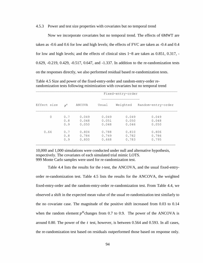
4.5.3 Power and test size properties with covariates but no
temporal trend ....................................................................................................... 94
4.5.4 Power and test size properties with covariates and temporal
trend .......................................................................................................... 95
4.5.5 Property of the confidence interval .................................................. 97
4.6 Application to a single trial data that mimic LOTS ................................ 97
4.7 Discussion ............................................................................................... 99
CHAPTER 5. CONCLUSIONS AND DISCUSSIONS ........................................... 104
Appendix A WinBUGS code for semicompeting risks model .................................. 107
Appendix B Simulating semicompeting risks data based on general models ........... 112
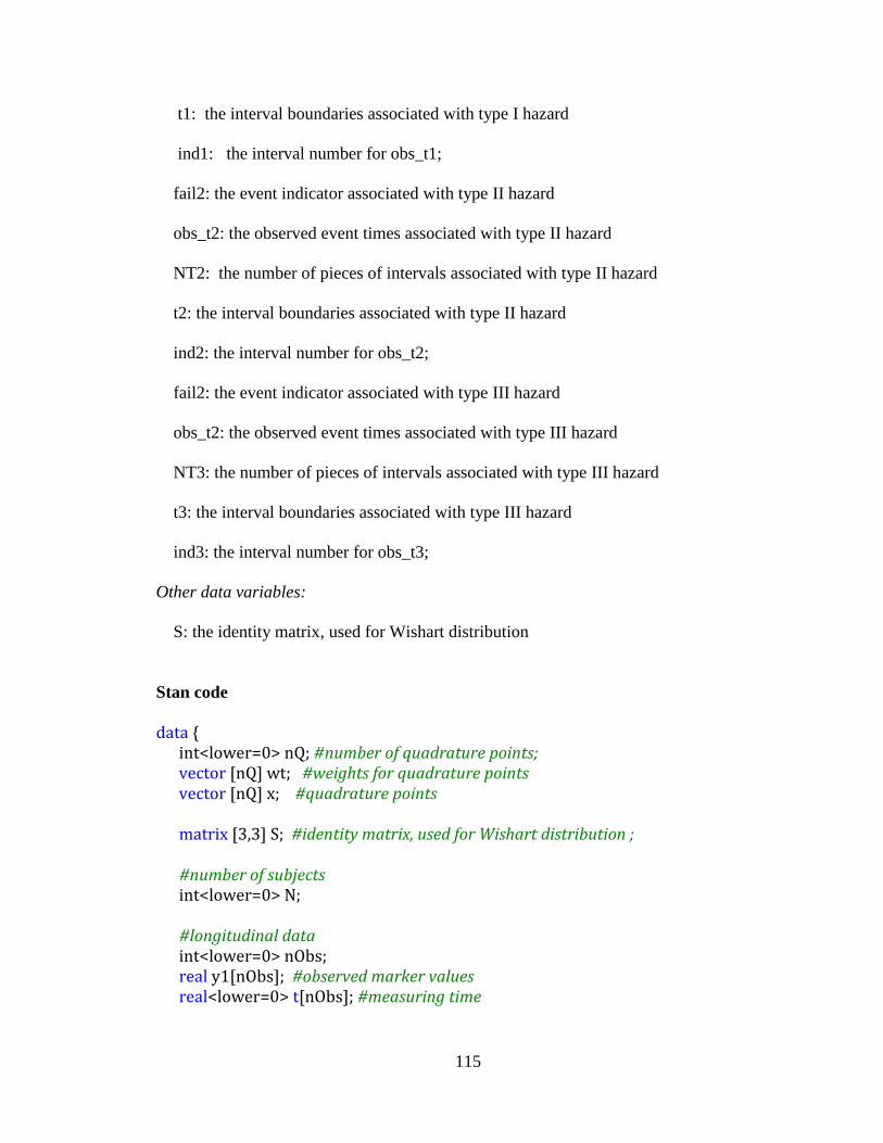
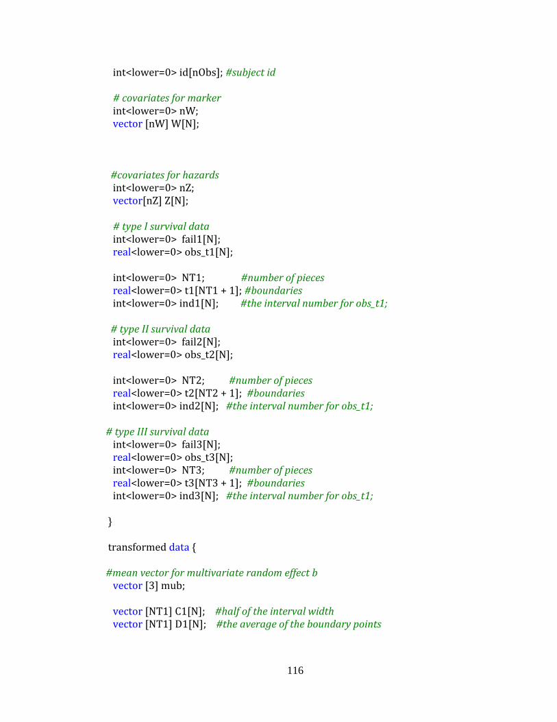
Appendix C Stan code for joint modeling ................................................................. 114
Appendix D Derivation of formula (4.4) and (4.5) .................................................... 122
BIBLIOGRAPHY ........................................................................................................... 124
CURRICULUM VITAE
Page 11
xi
LIST OF TABLES
...............................................................................................................................................
Table 2.1 Simulation results comparing parametric and semi-parametric Bayesian
models ............................................................................................................................... 24
Table 2.2 NSABP B-14 data analysis based on restricted models ................................... 27
Table 2.3 NSABP B-14 data analysis based on general models...................................... 29
Table 2.4 NSABP B-22 data analysis using restricted models ......................................... 34
Table 2.5 NSABP B-22 data analysis using general models ........................................... 36
Table 3.1 Parameter estimation for simulation studies based on various joint models .... 56
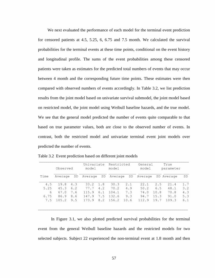
Table 3.2 Event prediction based on different joint models ............................................ 57
Table 3.3 Description of PSA data ................................................................................... 60
Table 3.4 Analysis results for the longitudinal submodels on PSA .................................. 63
Table 3.5 Survival submodels based on two-stage and simultaneously
joint modeling ................................................................................................................... 66
Table 4.1 Reference set for the fixed-entry-order re-randomization test .......................... 81
Table 4.2 Size and power for the fixed-entry-order re-randomization test following
minimization with no covariates and no temporal trend ................................................... 91
Table 4.3 Size and power of the fixed-entry-order and random-entry-order re-
randomization tests following minimization with no covariates and no temporal
trend .................................................................................................................................. 91
Table 4.4 Size and power for the fixed-entry-order re-randomization test following
minimization with covariates but no temporal trend ........................................................ 93
Table 4.5 Size and power of the fixed-entry-order and random-entry-order re-
randomization tests following minimization with covariates but no temporal trend ........ 94
Page 12
xii
Table 4.6 Size and power for the fixed-entry-order re-randomization test following
minimization with covariates but no temporal trend ........................................................ 95
Table 4.7 Type I error and average power of different re-randomization tests
following minimization with covariates in the presence of temporal trend ...................... 96
Page 13
xiii
LIST OF FIGURES
...............................................................................................................................................
Figure 2.1 Illness-death model framework ....................................................................... 13
Figure 2.2 The estimated baseline cumulative hazards for the NSABP B-14 dataset
based on the restricted and general semicompeting risks models ..................................... 30
Figure 2.3 Prediction of distant recurrence for a patient experienced the local failure .... 31
Figure 2.4 Prediction of distant recurrence for a patient who has not experienced
the local failure ................................................................................................................. 32
Figure 2.5 The estimated baseline cumulative hazards for the NSABP B-22
dataset based on the restricted and general semicompeting risks models ........................ 35
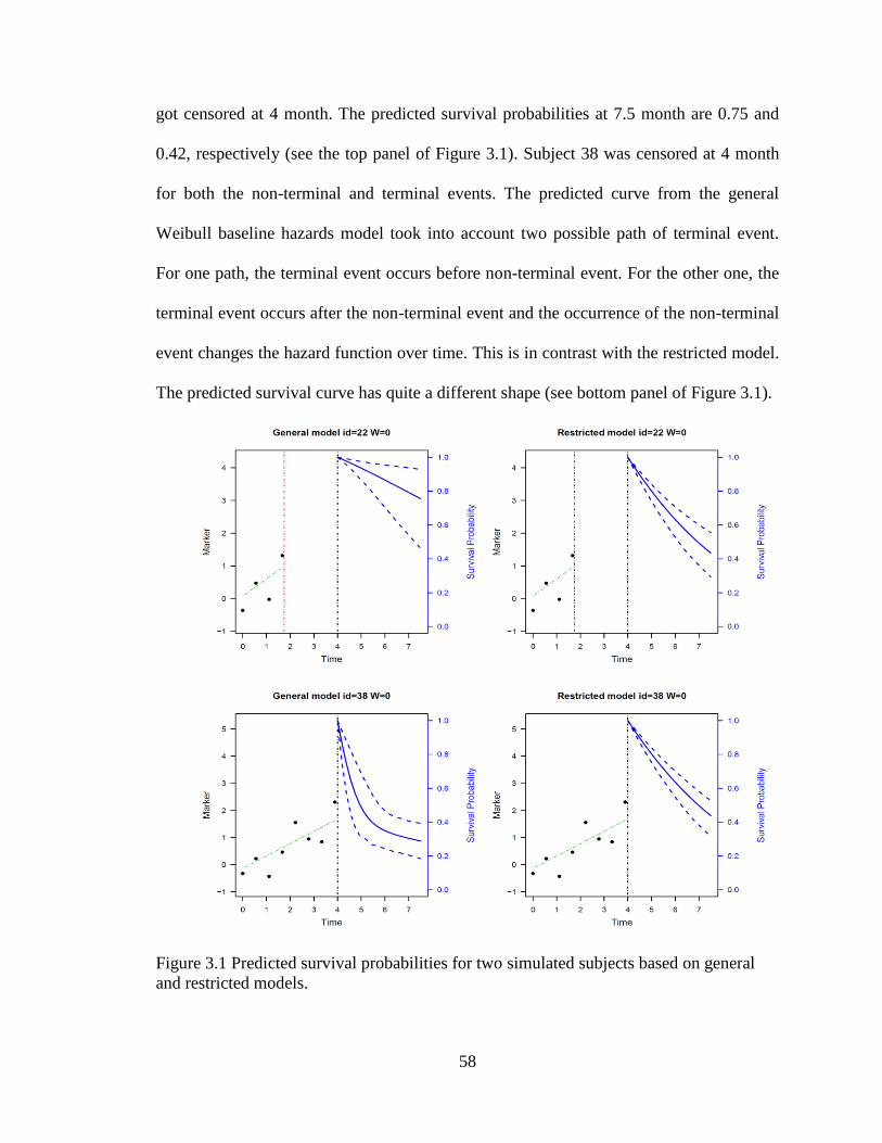
Figure 3.1 Predicted survival probabilities for two simulated subjects based on
general and restricted models............................................................................................ 58
Figure 3.2. Individual PSA profiles from randomly selected 50 patients (left) and
Kaplan-Meier curve on recurrence (right). ....................................................................... 59
Figure 3.3 Posterior marginals for selected parameters. ................................................... 62
Figure 3.4 Baseline survival based on joint models ......................................................... 65
Figure 3.5 Fitted PSA process and hazard process for early and late T-stage patients. ... 67
Figure 3.6 Prediction of survival for a patient receiving SADT ...................................... 68
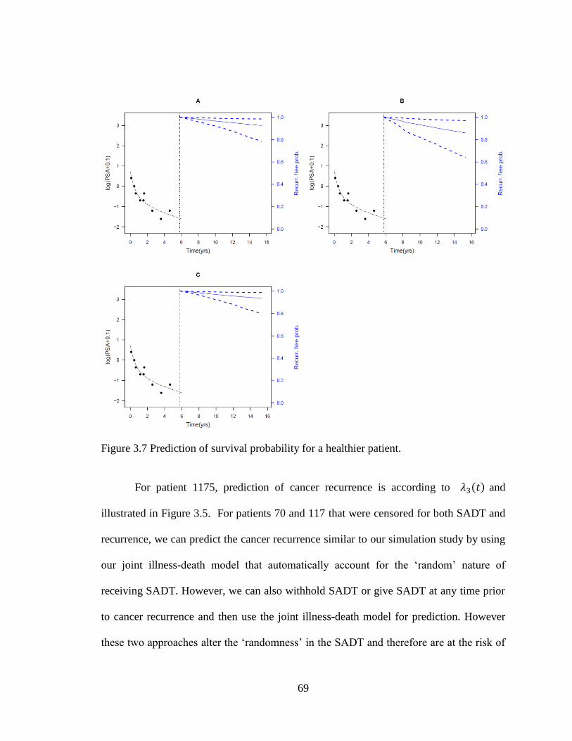
Figure 3.7 Prediction of survival probability for a healthier patient. ................................ 69
Figure 3.8 Prediction of survival probability for a sicker patient ..................................... 71
Figure 4.1 Representative examples of allocation probabilities of BCM in trials
that mimic LOTS. ............................................................................................................. 82
Figure 4.2 Comparison of the distributions of various re-randomization tests. ................ 90
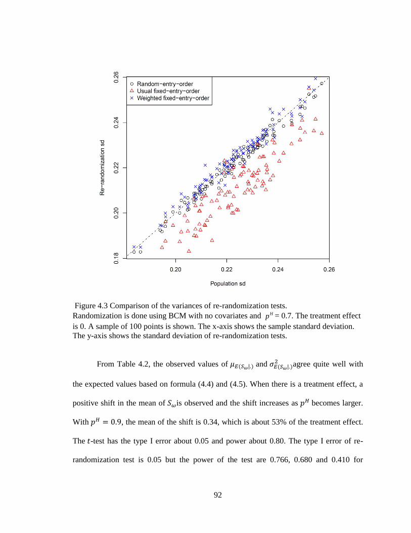
Figure 4.3 Comparison of the variances of re-randomization tests. ................................. 92
Page 14
xiv
Figure 4.4 Confidence interval estimation by re-randomization tests. ............................. 98
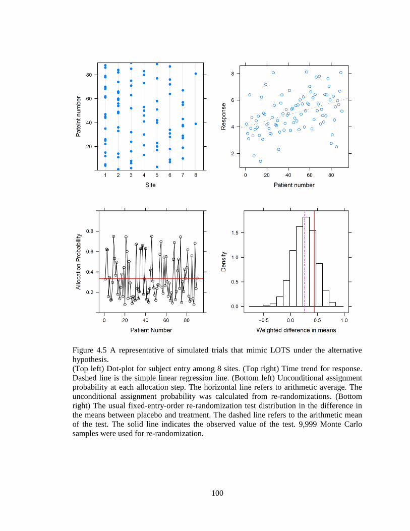
Figure 4.5 A representative of simulated trials that mimic LOTS under the
alternative hypothesis...................................................................................................... 100
...............................................................................................................................................
Page 15
1
CHAPTER 1. INTRODUCTION
Monte Carlo (MC) methods are a class of computational algorithms that rely on
repeated random sampling to compute quantities of interest. MC methods are widely used
to solve mathematical and statistical problems. These methods are mostly applicable
when it is infeasible to compute an exact result with a deterministic algorithm or when
theoretical close-form derivations are not possible.
In this dissertation, we will focus on two applications areas of MC methods: (i)
Bayesian modeling using Markov Chain Monte Carlo (MCMC) methods, with particular
focus on semicompeting risks data and joint models. (ii) Randomization-based inference,
with particular focus on an issue recently identified when subjects in clinical trials are
randomized with the minimization algorithm. Both topics are frequently encountered in
clinical trials. We developed and evaluated novel approaches for both problems.
First, we developed novel Bayesian approaches for flexible modeling of the
semicompeting risks data. The proposed method was applied to two breast cancer studies.
We then proposed a novel method for the joint modeling of the longitudinal biomarker
and semicompeting risks data. The method is applied to prostate cancer studies. Finally,
we discuss and evaluate a weighted method for randomization-based inference, which
overcomes a problem recently discovered in this field.
Page 16
2
1.1 Bayesian approach for semicompeting risks data
Semicompeting risks data arise when two types of events, non-terminal and
terminal, are observed. When the terminal event occurs first, it censors the non-terminal
event, but not vice versa.
Semicompeting risks data are frequently encountered in medical research. For
example, in oncology clinical trials comparing two treatments, the time to tumor
progression (non-terminal) and the time to death (terminal) of cancer patients from the
date of randomization are routinely recorded. As the two-types of events are usually
correlated, models for semicompeting risks should properly take account of the
dependence. In the literature, copula models are popular approaches for modeling of such
data. However, the copula model postulates latent failure times and marginal distributions
for the non-terminal event that may not be easily interpretable in reality. Further, the
development of regression models is complicated for copula models. To overcome these
issues, the well-known illness-death models have been recently proposed for more
flexible modeling of semicompeting risks data. The proposed model includes a gamma
shared frailty to account for the correlation between the two types of events. The use of
gamma frailty is for purposes of the mathematical simplicity. We therefore extend this
framework by proposing multivariate lognormal frailty models to incorporate random
covariates and capture heterogeneous correlation structures in the data.
The standard likelihood based approach for multivariate lognormal frailty models
involves multi-dimensional integrals over the distribution of the multivariate frailties,
which almost always do not have analytical solutions. Numerical solutions such as
Gaussian quadrature rules, Monte Carlo sampling have been routinely used in literature.
Page 17
3
However, as the dimension increases, these approaches still remain computationally
demanding.
Bayesian MCMC method has also been applied as estimation procedures for frailty
models. The MCMC method generates a set of Markov chains whose joint stationary
distribution corresponds to the joint posterior of the model, given the observed data and
prior distributions. With MCMC method, the frailty terms are treated as no different from
other regression parameters and the posterior of each parameter is approximated by the
empirical distribution of the values of the corresponding Markov chain. The use of
MCMC methods circumvents the complex integrations usually involved in obtaining the
marginal posterior distribution of each parameter. Due to the availability of general tools
for analyzing Bayesian models using MCMC methods, Bayesian methods is increasingly
popular for modeling of complex statistical problems. As another advantage, the event
prediction for survival models is very straightforward with Bayesian approach.
We therefore propose a practical Bayesian modeling approach for semicompeting
risks models. This approach utilizes existing software packages for model fitting and
future event prediction. The proposed method is applied to two breast cancer studies.
1.2 Joint modeling of repeated measures and semicompeting data
In longitudinal studies, data are collected on a repeatedly measured marker and a
time-to-event outcome. Longitudinal data and survival data are often associated in some
ways. Separate analysis of the two types of data may lead to biased or less efficient
results. In recent years, methods have been developed for joint models, where the
repeated measures and failure time are assumed to depend on a common set of random
effects. Such models can be used to assess the joint effects of baseline covariates (such as
Page 18
4
treatments) on the two types of outcome, to adjust the inferences on the repeated
measurements accounting for potential informative drop-out, and to study the survival
time for a terminating or recurrent event with measurement errors or missing data in time
varying covariates.
Despite the increasing popularity of joint models, the description of joint models
for longitudinal marker and semicompeting risks data is still scarce in literature. In this
dissertation, we extend our lognormal frailty models on the semicompeting risks data to
the joint modeling framework and develop a Bayesian approach. We applied our
approach to a prostate cancer study.
1.3 Weighted method for randomization-based inference
In the third part, we focused on randomization-based inference, a nonparametric
method for parameter estimation and inference, which is somewhat less related to the first
two topics. However, this method is especially important in clinical trial settings because
it makes minimum assumptions. It also represents another important area where Monte
Carlo method can be used.
For randomized clinical trials, the primary objective is to estimate and test the
comparative effects of the new treatment versus the standard of care. A well-run trial may
confirm a causal relationship between a new treatment and a desired outcome. In the
meantime, one can make inference on treatment effect based on the randomization
procedure, by which treatment assignments are produced for the study. The null
hypothesis of the randomization based tests is that the outcomes of subjects are not
affected by the treatments. Under this hypothesis, we re-run our experiments many
times, each time we reassign subjects to treatments but leave the outcomes unchanged to
Page 19
5
represent the hypothesis of no effects, and each time we record the difference of means
between the two treatments. From many such replications, we would obtain a set of
numbers that represent the distribution of the difference of means under null hypothesis.
And the inference can then be based on comparing the actual observation of the treatment
difference from the null distribution. Because it is usually computationally infeasible to
enumerate all permutations of the re-randomization process, a random Monte Carlo
sample is often used to represent the process.
In practice, subject randomization is seldom performed with the complete
randomization algorithm. Since a typical clinical trial usually includes a limited number
of subjects, the use of a complete randomization may leave a substantial imbalance with
respect to some important prognostic factors. Instead, some restricted randomization
procedures such as blocked randomization or minimization are proposed to balance
important prognostic factors that are known to affect the outcomes of the subjects. In
particular, minimization is a method of dynamic treatment allocation in a way to
minimize the differences among treatment groups with respect to predefined prognostic
factors.
When minimization is used as a procedure for randomization, the standard method
for randomization based inference works well when subjects are equally allocated to two
treatments. With an unequal allocation ratio, however, randomization inference in the
setting of minimization was found to be compromised in power. In this research, we
further investigated this issue and proposed a weighted method to overcome the problem
associated with unequal allocation ratio. Extensive simulations mimicking the setting of a
real clinical trial are performed to understand the property of the proposed method.
Page 20
6
This dissertation is organized as follows. In Chapter 2, we present our Bayesian
approach for semicompeting risks data. Chapter 3 develops the joint modeling of
longitudinal markers and semicompeting risks data. In Chapter 4, we propose and
evaluate the weighted approach for randomization based inference for clinical trials using
minimization procedure. Chapter 5 gives concluding remarks.
Page 21
7
CHAPTER 2. BAYESIAN APPROACH FOR SEMICOMPETING RISKS DATA
2.1 Summary
Semicompeting risks data arise when two types of events, non-terminal and
terminal, are observed. When the terminal event occurs first, it censors the non-terminal
event, but not vice versa. To account for possible dependent censoring of the non-
terminal event by the terminal event and to improve prediction of the terminal event
using the non-terminal event information, it is crucial to properly model their correlation.
Copula models are popular approaches for modeling such correlation. Recently it was
argued that the well-known illness-death models may be better suited for such data. We
extend this framework to allow flexible random effects to capture heterogeneous
correlation structures in the data. Our extension also represents a generalization of the
popular shared frailty models which only uses frailty terms to differentiate the hazards for
the terminal event without non-terminal event from those with non-terminal event. We
propose a practical Bayesian modeling approach that can utilize existing software
packages for model fitting and future event prediction. The approach is demonstrated via
both simulation studies and breast cancer data sets analysis.
Page 22
8
2.2 Introduction
Semicompeting risks data arise when two types of events, a non-terminal event (e.g.,
tumor progression) and a terminal event (e.g., death) are observed. When the terminal
event occurs first, it censors the non-terminal event. Otherwise the terminal event can still
be observed when the non-terminal event occurs first [1, 2]. This is in contrast to the
well-known competing risks setting where occurrence of either of the two events
precludes observation of the other (effectively censoring the failure times) so that only
the first-occurring event is observable. More information about the event times are
therefore contained in semicompeting risks data than typical competing risks data due to
the possibility of continued observation of the terminal event after the non-terminal event.
Consequently, this allows modelling of the correlation between the non-terminal and
terminal events without making strong assumptions. Adequate modelling of the
correlation is important to address the issue of dependent censoring of the non-terminal
event by the terminal event [2-4]. It also can allow modelling of the influence of the non-
terminal event on the hazard of the terminal event and thus improve on predicting the
terminal event [5].
Semicompeting risks data are frequently encountered. For example, in oncology
clinical trials, time to tumor progression and time to death of cancer patients from the
date of randomization are normally recorded. It is generally expected that the two event
times are strongly correlated. Main objectives of the trials usually include estimation of
treatment effects on both of these events. When the time to death is the primary endpoint,
there may also be great interest in predicting the overall survival based on disease
progression to facilitate more efficient interim decisions in subsequent clinical trials [5].
Page 23
9
Dignam et al. [6] presented randomized breast cancer clinical trials with data collection
of first recurrence at any anatomic site (local, regional, or distant) as well as the first
distant recurrence. If the local recurrence occurs first, patients will continue to be
followed up for the first recurrence at distant location and hence both types of events may
be observed. When the local failure occurs after distant failures, however, the local
recurrence is usually not rigorously ascertained in practice. Another semicompeting data
example is AIDS studies where the non-terminal event is first virologic failure and the
terminal event is treatment discontinuation [7].
Semicompeting risks data have been popularly modeled using copula models [1-4,
8-15]. The copula model includes nonparametric components for the marginal
distributions of the two types of events and an association parameter to accommodate
dependence. Despite its flexibility, regression analysis is somewhat awkward under the
copula framework. Peng (2007) and Hsieh (2008) proposed separate marginal regression
models for the time to the terminal and non-terminal events and a possibly time-
dependent correlation parameter[12, 14]. In this approach, the marginal regression for the
terminal event is first estimated, for example via the Cox proportional hazards model.
Then, the marginal regression for the non-terminal event and the association parameter in
the copula are jointly estimated by estimating equations. To gain efficiency, Chen [16]
developed a likelihood-based method. A similar approach to incorporate time-dependent
covariates in copula models was also developed [17].
Another bothersome feature of the copula models is that they are specified in terms
of the latent failure time for the non-terminal event. Supposition of such a failure event
may be unnatural, similar to the problem arising in the classical competing risks setting
Page 24
10
[18]. Consequently Xu et al. [18] suggested the well-known illness-death models to
tackle both issues. Their approach not only allows for easy incorporation of covariates
but also is based only on observable quantities; no latent event times are introduced.
Their general illness-death models differentiate three types of hazards: hazard of illness,
hazard of death without illness and hazard of death with illness. Incorporation of
covariates is achieved through proportional hazards modeling. A single gamma frailty
term is used to model the correlation among different hazards corresponding to the two
types of events. Nonparametric maximum likelihood estimation (NPMLE) based on
marginalized likelihood is used for inference.
The gamma frailty in the proposed illness-death model is used mainly for
mathematical convenience, namely because it leads to closed-form expressions of the
marginal likelihood. In addition to the restriction of using a single variable to capture all
associations, it is also hard to extend the gamma frailty framework to incorporate
covariates or random effects into modeling the correlation structure. Other distributional
models have been suggested for frailty [19]. Among them, the log-normal frailty models
are especially suited to incorporate covariates [20-26]. With the log-normal frailty, it is
very easy to create correlated but different frailties as required in correlated frailty
models [23]. We therefore extend the gamma frailty model of Xu et al. (2010) to log-
normal frailty models to comprehensively model the correlation among the hazard
functions. Our extension also represents a generalization of the popular shared frailty
models for joint modelling of non-terminal and terminal events [25, 27]. These shared
frailty models belong to the ‘restricted model’ in the terminology of Xu et al. (2010)
because they do not differentiate the hazards for the terminal event without non-terminal
Page 25
11
event from those with non-terminal event. As a result, shared frailty models tend to put
very strong assumptions on the correlation structure and may be inadequate to capture as
much data heterogeneity, similar to the longitudinal data analysis setting [28]. In contrast,
our adopted ‘general model’ assumes that the terminal event hazard function is possibly
changed after experiencing the non-terminal event on top of the frailty terms.
With the log-normal frailty model, it is unfortunately impossible to derive the
marginal likelihood function in an explicit form, and as such, parameter estimation needs
to resort to different numerical algorithms [26]. In this chapter, we propose using
Bayesian Markov Chain Monte Carlo methods (MCMC) to directly work with the full
likelihood. The Bayesian MCMC methods have been applied as estimation procedures in
frailty models [23, 29-32]. The Bayesian paradigm provides a unified framework for
carrying out estimation and predictive inferences. In particular, we show that
computation can be carried out using existing software packages such as WinBUGS [33],
JAGS [34], and Stan [35], which leads to simple implementation of the modelling
process. In Section 2.3 we describe the model formulation. In Section 2.4, we present
details of the Bayesian analysis including prior specification, implementation of the
MCMC, and computation using existing software packages. In Section 2.5, we present
results from some simulation studies. In Section 2.6, we conduct a thorough analysis of
two breast cancer clinical trial datasets. Section 2.7 contains a brief discussion.
2.3 Model formulation
Let be the time to the non-terminal event, e.g., disease progression (referred to
as illness hereafter), be the time to the terminal event (referred as death hereafter), and
be the time to the censoring event (e.g., the end of a study or last follow-up assessment
Page 26
12
status). Observed variables consist of , ,
, and . Note that can censor but not vice visa, whereas can
censor both and . Semicompeting risks data such as these can be conveniently
modelled using illness-death models [18]. These models assume individuals begin in an
initial healthy state (state 0) from which they may transition to death (state 2) directly or
may transit to an illness state (state 1) first and then to death (state 2) (see Figure 2.1) .
The hazards or transition rates are defined as follows:
(2.1)
(2.2)
(2.3)
where . Equations (2.1) and (2.2) are the hazard functions for illness and
death without illness, which are the competing risks part of the model. Equation (2.3)
defines the hazard for death following illness. In general, can depend on both
and . These equations define a semi-Markov model. When , the
model becomes Markov. The ratio partly explains the dependence
between and . When this ratio is 1, the occurrence of has no effect on the hazard
of . Borrowing the terminology from Xu et al. [18], we refer models that force
as “restricted models” and models without this assumption as
“general” models.
To account for the dependency structure between and , Xu et al. (2010)
introduced a single shared gamma frailty term to capture correlation among ,
Page 27
13
and . Here we extend to model the correlation using multivariate random
variables. In particular, we specify the following conditional transition functions:
Figure 2.1 Illness-death model framework
(2.4)
(2.5)
(2.6)
where , and are the unspecified baseline hazards; , and
are vectors of regression coefficients associated with each hazard; , , and are
subsets of and may have overlap with each other; and , , and are subsets of
and may have overlap with each other or with , , and .
Models (2.4) - (2.6) allow multivariate random effects with arbitrary design matrix
in the log relative risk. In its simplest form, when , the frailty term is
reduced to a univariate random variable that accounts for the subject-specific dependency
of three types of hazards. The models in Xu et al. (2010) belong to this simple case where
they assume that ) follows a gamma distribution. However, in many cases, random
effects based on covariates, e.g., clinical center or age, may provide better models for the
Page 28
14
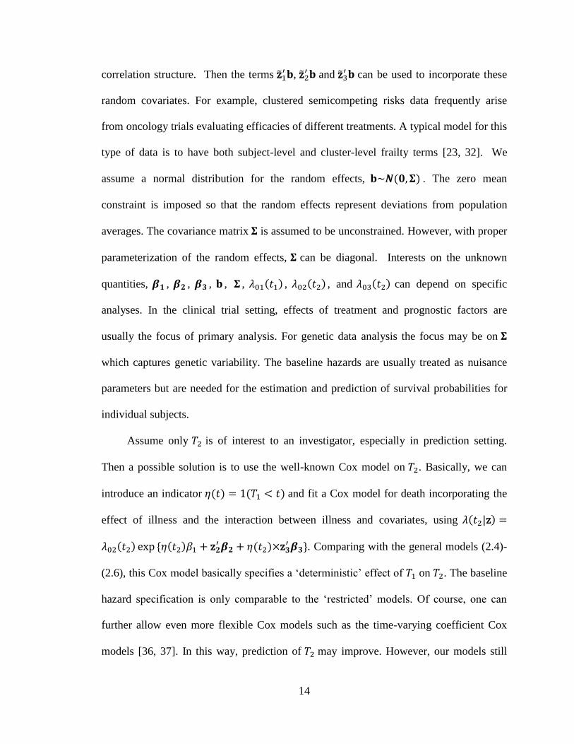
correlation structure. Then the terms ,
and can be used to incorporate these
random covariates. For example, clustered semicompeting risks data frequently arise
from oncology trials evaluating efficacies of different treatments. A typical model for this
type of data is to have both subject-level and cluster-level frailty terms [23, 32]. We
assume a normal distribution for the random effects, . The zero mean
constraint is imposed so that the random effects represent deviations from population
averages. The covariance matrix is assumed to be unconstrained. However, with proper
parameterization of the random effects, can be diagonal. Interests on the unknown
quantities, , , , , , , , and can depend on specific
analyses. In the clinical trial setting, effects of treatment and prognostic factors are
usually the focus of primary analysis. For genetic data analysis the focus may be on
which captures genetic variability. The baseline hazards are usually treated as nuisance
parameters but are needed for the estimation and prediction of survival probabilities for
individual subjects.
Assume only is of interest to an investigator, especially in prediction setting.
Then a possible solution is to use the well-known Cox model on . Basically, we can
introduce an indicator and fit a Cox model for death incorporating the
effect of illness and the interaction between illness and covariates, using
. Comparing with the general models (2.4)-
(2.6), this Cox model basically specifies a ‘deterministic’ effect of on . The baseline
hazard specification is only comparable to the ‘restricted’ models. Of course one can
further allow even more flexible Cox models such as the time-varying coefficient Cox
models [36, 37]. In this way, prediction of may improve. However, our models still
Page 29
15
offer more flexibility in capturing underlying data heterogeneity and prediction. In
particular, for any subject without illness, we can incorporate the illness progression via
model (2.5) and (2.6) in predicting .
Note that the general models allow much flexibility in model specification in case
of prior scientific knowledge or data sparsity. For example, we can set
but still allow different covariates in (2.5) and (2.6). The models can also easily
incorporate time-dependent covariates. For example, if interventions such as drugs or
behaviorial change were taken, for example, sometime after illness, then an indicator for
the intervention can be incorporated into in (2.6). However care must be taken
to identifiability issues. If all subjects take drugs immediately after illness, then the drug
effect is confounded with the baseline hazard . In this case, we need to put
constraints on , such as in order to estimate the drug effect.
For a subject , we observe , , Let
, , and be
the counting processes for the three patterns of the event process. Correspondingly, let
and be the
at-risk process for the three types of events. We assume that the censoring time is
independent of , , given covariates
For the subject i, the likelihood is
. The likelihood can be simplified to
. Note that
Page 30
16
when , and therefore the last part of can also be written as
. From the definition of the hazard functions, we can obtain
expressions of the probabilities by solving the corresponding ordinary differential
equations that link these hazards to distribution functions. Specifically, we have
By plugging the above two equations into and multiply across all subjects, we
obtain the following likelihood,
∏
With the proportional hazards assumptions and the use of counting process notations,
the corresponding likelihood can be rewritten as,
(2.7) ∏ ∏ {∏
[ ∫
]}
where
,
,
and
.
We can view (2.7) as Poisson kernels for the random variables with means
of . That is, . More specifically, the joint likelihood
can be written as
Page 31
17
(2.8)
∏[
] [
]
∏[
]
[
]
∏[
]
[
]
where are the baseline cumulative hazards functions.
Note that with the restricted model, the likelihood in (2.8) reduces to
(2.9)
∏ [
] [
]
∏ [
] [
]
The baseline hazard functions are left unspecified. Similar to Zeng and Lin
(2007) [25], we take as a discrete function, or as a step function, with
increments or jumps occurring at the corresponding observed distinct failure time points.
In other words, for , its jump points are at those with ; for , its
jump points are at those with and ; and for , its jump points are
at those with and . The jump sizes are treated as parameters in
maximizing (2.8). When the sample sizes are small or the number of events is low, the
need to estimate such a large number of parameters may lead to computational instability.
Page 32
18
In this case we can also model the baseline hazards from parametric distributions such as
the exponential, Weibull, lognormal, etc. However, these parametric assumptions can be
too restrictive. An attractive compromise is to adopt piecewise constant (PWC) baseline
hazards models to approximate the unspecified baseline hazards, which may significantly
reduce computational time [38]. For , the follow-up times are divided into
intervals with break points at where equals or exceeds the largest
observed times and . Usually, is located at the th quantile of the observed
failure times. The baseline hazard function then takes values in the intervals
] for .
2.4 Bayesian approach
Estimation for frailty models can usually be conducted using either the expectation-
maximization (EM) algorithm [25, 39-41] or MCMC methods [23, 29, 42-48]. When the
EM algorithm is used, the unobserved random effects are treated as ‘missing values’ in
the E step. The conditional expectations of random effects often involve intractable
integrals and Monte Carlo methods have been used to approximate the integrals [26, 27,
43]. The implementation of Monte Carlo EM becomes less straightforward and usually
needs to be treated on a case-by-case basis. For semicompeting risks data, involvement of
different event types will make programming a daunting task that can easily discourage
ordinary users. In addition, for prediction of future events, high order integration
involving complicated functions of random effects is needed under the EM algorithm.
Other numerical methods for maximizing likelihood were also proposed.
McGilchrist and Aisbett (1991) first adopted the partial penalized likelihood (PPL)
method for frailty models [20, 21]. In the simple frailty structure, the PPL estimation
Page 33
19
works relatively well. With multidimensional random effects, a two-step procedure was
proposed based on simple estimating equations and a penalized fixed effects partial
likelihood [49]. However, this approach leads to an underestimation of the variability of
the fixed parameters. Liu et al. [38] proposed a Gaussian quadrature estimation method
for restricted joint frailty models with a single frailty term using the piecewise constant
baseline hazard functions. Estimation can then be implemented easily in SAS. However,
when the baseline hazard is left unspecified, this approach does not work with the
existing software anymore. In addition, generalization of their method to our general
model may be difficult.
We therefore utilizes to a Bayesian approach for computation. Bayesian MCMC
methods have been applied as estimation procedures for frailty models [23, 29-32]. The
Bayesian framework is naturally suited to our setting with conditionally independent
observations and hierarchical models. The Bayesian approach allows us to use existing
software packages like WinBUGS [33], JAGS [34], and Stan [35]. The model fitting
becomes very accessible to any users. For example, the program for WinBUGS only
involved tens of lines (see Appendix A).
In order to carry out the Bayesian analysis, we specify the prior distributions for
various parameters as follows. Following Kalbfleisch [50], the priors for are
assigned as gamma processes with means and variances
for k=1, 2, 3.
The increments are distributed as independent gamma variables with shape and
scale parameters and , respectively.
can be viewed as an initial
estimate of . The scale reflects the degree of belief in the prior specification
with smaller values associated with higher levels of uncertainty. In our computation, we
Page 34
20
take . For univariate censored survival data without any frailty term, the prior
for has the virtue of being conjugate and the Bayes estimator (given ) for
is a shrinkage estimator between the maximum likelihood estimate and the prior
mean [29]. In our computation, we take the mean process
to be
proportional to time, that is, with . With this formulation, can be
considered as the mean baseline hazard rate.
For regression parameters, independent normal prior distributions are assigned
with as the corresponding identity matrices for . Usually,
large values of
are used so that the prior distributions bear negligible weights on the
analysis results. However relevant historical information about regression parameters can
be incorporated into the prior distribution to enhance the analysis results.
Finally, we specify an inverse Wishart prior distribution for the unconstrained
covariance matrix, . To represent non-informative prior, we choose the
degree of freedom of this distribution as d, i.e. the rank of , which is the smallest
possible value for this distribution. The scale matrix is often chosen to be an identity
matrix multiplied by a scalar . The choice of is fairly arbitrary. The sensitivity of the
results to changes of needs to be examined to ensure the prior distribution can leave
considerable prior probabilities for extreme values of the variances terms. If we have
evidence to assume no correlation among the random effects, diffuse priors can be
directly specified on the diagonal elements of : for . With
minimum prior information, we can choose and . For the piecewise
constant baseline models, diffuse gamma distribution priors can be specified for ,
Page 35
21
for .With minimum prior information, we can choose
and .
Because the posterior distributions involve complex integrals and are
computationally intractable, MCMC methods are used. The existing packages WinBUGS,
JAGS, and Stan all led to similar results in our simulation studies. Our analysis was based
on Stan version 1.1.0 [35], an open-source generic BUGS-style [51] package for
obtaining Bayesian inference using No-U-Turn sampler[52], a variant of the Hamiltonian
Monte Carlo[53]. For complicated models with correlated parameters, the Hamiltonian
Monte Carlo avoids the inefficient random walks used in simple MCMC algorithms such
as the random-walk Metropolis [54] and Gibbs sampling [55] by taking a series of steps
informed by first-order gradient information, and hence converges to high-dimensional
target distributions more quickly [56]. However we provide the WinBUGS program
codes for the general Cox model and the PWC exponential model in Appendix A due to
the long-standing status of WinBUGS. Program codes for other packages are available
upon request.
Within the Bayesian framework it is straightforward to predict an individual’s
survival that is often of great interest to both patients and physicians. Denote
. The survival probability at time for a patient with illness at and
censored for death at is
Page 36
22
(2.10)
∫
∫
∫
∫ [
]
Direct evaluation of (2.10) can be very computationally challenging even when the
dimension of and are moderately high. Because we have draws of and from
the posterior distribution,
and for , a straightforward
approximation of (2.10) is via a simple sum with the following form:
∑ ( |
)
Similarly the survival probability for terminal event at time for a patient who is
censored for both illness and death events at is
(2.11)
∫
∫
∫
Where
[ {
} ]
[ {
} ]
Page 37
23
∫
∫
Again (2.11) may be approximated by ,
∑ ( |
) .
2.5 Simulation study
We generated data according to models (2.4) - (2.6) with the Weibull baseline
hazard functions in our simulation. Specifically we chose
and . A fixed covariate applies to all three models, with
corresponding coefficients and Random effects were
incorporated using and with the corresponding frailties generated
independently using normal distributions with variances of 1 and 0.8 respectively. The
censoring time is fixed at 3. The detailed methods for generating survival times based
on the general semicompeting risks models are given in Appendix B.
Page 38
24
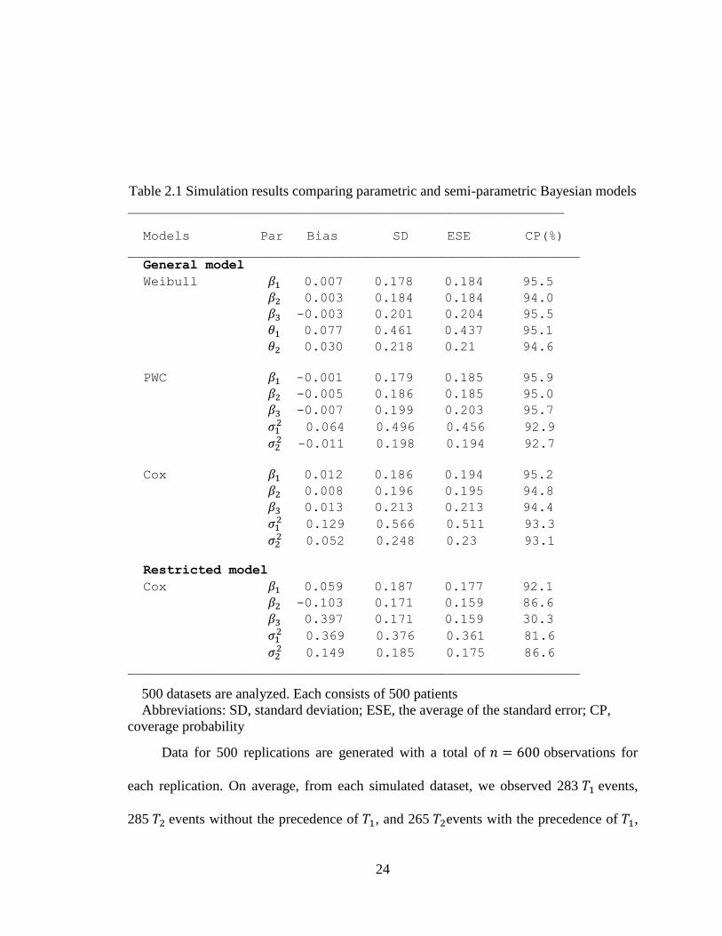
Table 2.1 Simulation results comparing parametric and semi-parametric Bayesian models ________________________________________________________
Models Par Bias SD ESE CP(%)
__________________________________________________________
General model
Weibull 0.007 0.178 0.184 95.5
0.003 0.184 0.184 94.0
-0.003 0.201 0.204 95.5
0.077 0.461 0.437 95.1
0.030 0.218 0.21 94.6
PWC -0.001 0.179 0.185 95.9
-0.005 0.186 0.185 95.0
-0.007 0.199 0.203 95.7
0.064 0.496 0.456 92.9
-0.011 0.198 0.194 92.7
Cox 0.012 0.186 0.194 95.2
0.008 0.196 0.195 94.8
0.013 0.213 0.213 94.4
0.129 0.566 0.511 93.3
0.052 0.248 0.23 93.1
Restricted model
Cox 0.059 0.187 0.177 92.1
-0.103 0.171 0.159 86.6
0.397 0.171 0.159 30.3
0.369 0.376 0.361 81.6
0.149 0.185 0.175 86.6
__________________________________________________________
500 datasets are analyzed. Each consists of 500 patients
Abbreviations: SD, standard deviation; ESE, the average of the standard error; CP,
coverage probability
Data for 500 replications are generated with a total of observations for
each replication. On average, from each simulated dataset, we observed 283 events,
285 events without the precedence of , and 265 events with the precedence of ,
Page 39
25
respectively. The analyses were conducted using the Cox models, the PWC exponential
models and the Weibull models for the baseline hazards. In addition to the general
models, the restricted Cox models were also fitted.
The results are summarized in Table 2.1. The average biases (Bias), the standard
deviation (SD) of the posterior mean, the average values of the estimated standard errors
(ESE), and coverage probabilities (CP) of the 95% credible intervals including the true
value are listed in the table. We can see that the three methods perform well for
regression and frailty parameters. In particular, the PWC exponential models are quite
comparable with Weibull models for both bias and SD estimates. The biases are small,
ESEs agree well with the sample SDs, and CPs are close to the nominal values. As
expected, ESEs and SDs increase with more complex models. The restricted Cox models
give an unbiased estimate for . However, the mean estimates for and is 0.897,
which is between the true values of and . This model does not consider differential
covariate effects. Further the variance estimates for random effects showed larger bias
compared with the general Cox models. The inflation of the variance may be attributed to
the misspecification (or restriction) of the baseline hazards which confounds the frailty
terms. We used Stan to perform all the simulations. With 10,000 posterior samples and
2,000 burn-in iterations, it took an average of 5.5 minutes per data set analysis for the
Weibull models, 7.3 minutes for the PWC exponential models with 20 pieces and 39.5
minutes for the Cox models on Linux server with 2.40 GHz Intel Xeon E7340 CPU and
4.0 GB RAM. Three multiple chains were run in parallel and the method of Gelman-
Rubin was used for convergence diagnosis[57].
Page 40
26
2.6 Application to breast cancer data
2.6.1 Effect of tamoxifen on local-regional failure in node-negative breast cancer
Between 1982 and 1988, 2892 women with estrogen receptor-positive breast
tumors and no auxiliary node involvement were enrolled in National Surgical Adjuvant
Breast and Bowel Project (NSABP) Protocol B-14, a double-blind randomized trial
comparing 5 years of tamoxifen (10 mg b.i.d.) with placebo [6, 58]. Women in the study
were observed for recurrence at local-regional, or distant sites. If distant metastasis was
the first event, then reporting of additional local-regional failure was not required.
Consequently, the data follow the semicompeting risks structure where the local-regional
failure is considered as non-terminal and distant failure as terminal [6]. Among 2850
patients with follow-up times of at least 6 months before any events, 1424 and 1426
patients received placebo and tamoxifen, respectively. A total of 237 patients had local
recurrence and 93 of them further developed distant metastasis. A total of 428 patients
had distant recurrence without local-regional failure occurring first.
We first fit a restricted model based on likelihood (2.9) to compare the effect of the
treatment. Covariates considered were age and tumor size at randomization. We
considered a shared frailty model with no random covariates. The results are summarized
in Table 2.2. As compared with placebo, tamoxifen significantly reduces both local and
distant recurrences with estimated log hazard ratios of -1.274 (95% credible interval (CI):
-1.642, -0.938) and -0.713 (95% CI: -1.019, -0.443), respectively. Both age and tumor
size have substantial effects on recurrences. Younger women have greater chance of
recurrence. It is true in general that younger women have worse prognosis, as younger
age at onset is associated with more aggressive tumor types. Every increase of 10 years in
Page 41
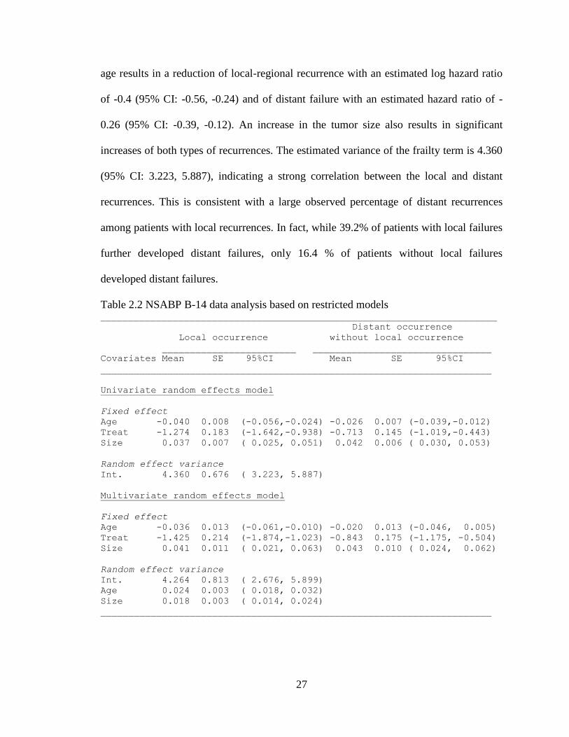
27
age results in a reduction of local-regional recurrence with an estimated log hazard ratio
of -0.4 (95% CI: -0.56, -0.24) and of distant failure with an estimated hazard ratio of -
0.26 (95% CI: -0.39, -0.12). An increase in the tumor size also results in significant
increases of both types of recurrences. The estimated variance of the frailty term is 4.360
(95% CI: 3.223, 5.887), indicating a strong correlation between the local and distant
recurrences. This is consistent with a large observed percentage of distant recurrences
among patients with local recurrences. In fact, while 39.2% of patients with local failures
further developed distant failures, only 16.4 % of patients without local failures
developed distant failures.
Table 2.2 NSABP B-14 data analysis based on restricted models _______________________________________________________________________
Distant occurrence
Local occurrence without local occurrence
________________________ ________________________________
Covariates Mean SE 95%CI Mean SE 95%CI
______________________________________________________________________
Univariate random effects model
Fixed effect
Age -0.040 0.008 (-0.056,-0.024) -0.026 0.007 (-0.039,-0.012)
Treat -1.274 0.183 (-1.642,-0.938) -0.713 0.145 (-1.019,-0.443)
Size 0.037 0.007 ( 0.025, 0.051) 0.042 0.006 ( 0.030, 0.053)
Random effect variance
Int. 4.360 0.676 ( 3.223, 5.887)
Multivariate random effects model
Fixed effect
Age -0.036 0.013 (-0.061,-0.010) -0.020 0.013 (-0.046, 0.005)
Treat -1.425 0.214 (-1.874,-1.023) -0.843 0.175 (-1.175, -0.504)
Size 0.041 0.011 ( 0.021, 0.063) 0.043 0.010 ( 0.024, 0.062)
Random effect variance
Int. 4.264 0.813 ( 2.676, 5.899)
Age 0.024 0.003 ( 0.018, 0.032)
Size 0.018 0.003 ( 0.014, 0.024)
______________________________________________________________________
Page 42
28
We next fit a restricted model with random covariates. The results are also shown in
Table 2.2. In addition to the random intercept, age and tumor size were included as
random covariates. An unstructured matrix was used to model the covariance of the
random effects. The posterior means of covariance were found to be rather close to zero
(data not shown), indicating minimum correlation among the random effects. The
variance for the random intercept, age and tumor size were quite different from zero, with
95% CIs of (2.676, 5.899), (0.018, 0.032), and (0.014, 0.024) respectively. The posterior
means of the log-hazard ratios of the treatment were -1.425 and -0.843 for the local and
distant recurrences respectively.
We also fit three general models based on (2.8): the random intercept Cox model,
the random effects Cox model and the random effects PWC model. The random effects
models used both age and tumor size as random covariates. Results are presented in
Table 2.3.
Based on the random intercept Cox model, the estimated cumulative baseline
hazards are plotted in Figure 2.2. In addition, for comparison, the estimated cumulative
baseline hazards based on restricted models are plotted in the same figure. Notice that the
restricted models do not distinguish the two types of hazards for the terminal events while
the general models do. The cumulative hazards for distant failure with and without local
recurrence are quite similar before 40 months, but then diverge from each other. The
variance of the random intercept is 2.617 with a standard error of 1.143, which is smaller
than that from the restricted model, possibly because the dependence of on is partly
captured by the different baseline hazard functions and .
Page 43
29
Table 2.3 NSABP B-14 data analysis based on general models ____________________________________________________________________________________________________
Distant occurrence Distant occurrence
Local occurrence without local occurrence after local occurrence
Covariates _________________________ __________________________ ____________________________
Mean SE 95%CI Mean SE 95%CI Mean SE 95%CI
______________________________________________________________________________________________________
Univariate random effects Cox model
Fixed effect
Age -0.035 0.008 (-0.051,-0.018) -0.022 0.007 (-0.037,-0.010) -0.007 0.015 (-0.036, 0.023)
Size 0.030 0.008 ( 0.017, 0.046) 0.035 0.007 ( 0.024, 0.049) 0.028 0.013 ( 0.004, 0.055)
Random effect variance
Intercept 2.617 1.143 1.025 5.353
Multivariate random effects Cox model
Fixed effect
Age -0.043 0.017 (-0.077,-0.012) -0.029 0.016 (-0.063, 0.001) -0.005 0.023 (-0.050, 0.041)
Treat -1.723 0.252 (-2.242,-1.236) -1.190 0.223 (-1.648,-0.766) -0.563 0.416 (-1.370, 0.215)
Size 0.052 0.014 ( 0.025, 0.079) 0.055 0.014 ( 0.028, 0.083) 0.050 0.019 ( 0.010, 0.087)
Random effect variance
Intercept 8.733 1.693 (5.753,12.619)
Age 0.032 0.006 ( 0.022, 0.044)
Size 0.023 0.004 ( 0.017, 0.031)
Multivariate random effects PWC model
Fixed effect
Age -0.043 0.015 (-0.073,-0.013) -0.029 0.015 (-0.059, 0.002) -0.003 0.023 (-0.047, 0.044)
Treat -1.658 0.245 (-2.173,-1.185) -1.126 0.228 (-1.613,-0.707) -0.451 0.409 (-1.258, 0.370)
Size 0.049 0.013 ( 0.024, 0.074) 0.051 0.013 ( 0.027, 0.075) 0.045 0.018 ( 0.010, 0.082)
Random effect variance
Intercept 7.635 1.689 (4.312,10.804)
Age 0.030 0.005 (0.022, 0.041)
Size 0.022 0.004 (0.016, 0.031)
_______________________________________________________________________________________________________
Page 44
30
Figure 2.2 The estimated baseline cumulative hazards for the NSABP B-14 dataset based
on the restricted and general semicompeting risks models
Based on the general model with only a random intercept, tamoxifen has a
significant effect in reducing the local-regional recurrence with an estimated log hazard
ratio of -1.130 (95% CI: -1.512, -0.802). Tamoxifen also has a significant effect on
distant recurrence without local failure with an estimated log hazard ratio of -0.616 (95%
CI: -0.949, -0.340). However, tamoxifen showed no effects in reducing distant recurrence
following local failure. This makes sense from a clinical and biological perspective.
Local failures tend to happen earlier than distant failures. If the tamoxifen fails to
control recurrence locally, then it also would likely not be able to control the distant
disease. The increase in tumor size has a comparable effect in increasing all three types of
recurrences. Age has a significant effect on both local and distant failure without local
reoccurrence, but no significant effect on distant recurrence following local failure,
indicating an age-independent metastatic rate after local failure. The fitted variances of
the random effects all differ from zero. The correlations among the three random effects
Page 45
31
are negligible. Similar conclusions about tamoxifen can be drawn as the random intercept
only model. In addition, the estimates based on the PWC exponential models are quite
comparable to the Cox models.
Figure 2.3 Prediction of distant recurrence for a patient experienced the local failure
Page 46
32
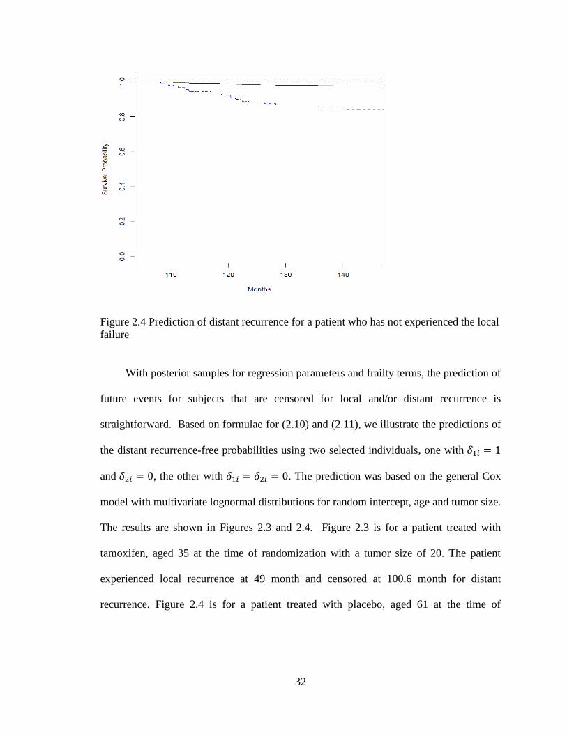
Figure 2.4 Prediction of distant recurrence for a patient who has not experienced the local
failure
With posterior samples for regression parameters and frailty terms, the prediction of
future events for subjects that are censored for local and/or distant recurrence is
straightforward. Based on formulae for (2.10) and (2.11), we illustrate the predictions of
the distant recurrence-free probabilities using two selected individuals, one with
and , the other with . The prediction was based on the general Cox
model with multivariate lognormal distributions for random intercept, age and tumor size.
The results are shown in Figures 2.3 and 2.4. Figure 2.3 is for a patient treated with
tamoxifen, aged 35 at the time of randomization with a tumor size of 20. The patient
experienced local recurrence at 49 month and censored at 100.6 month for distant
recurrence. Figure 2.4 is for a patient treated with placebo, aged 61 at the time of
Page 47
33
randomization with a tumor size of 33. The patient was censored at 107.9 months for
both types of recurrences.
2.6.2 Local-regional failure after surgery and chemotherapy for node-positive breast
cancer
NSABP Protocol B-22 is a randomized clinical trial to evaluate dose intensification
and increased cumulative dose on disease-free survival and survival of primary breast
cancer patients with positive auxiliary nodes receiving postoperative adriamycin-
cyclophosphamide (AC) therapy [59]. Between 1988 and 1991, 2305 women were
randomized and the primary trial findings indicated no advantage for increased or
intensified dose relative to the standard dose. However, this randomized trial provided
data for analyzing several important prognostic factors for failures, including the number
of lymph nodes that contained tumor cells (integer values from 1 to 37), size of the
primary tumor (in millimeters), and age at diagnosis. In our analysis, we included data
from 2201 patients with complete information for these covariates. Among these patients,
320 experienced local failures, 189 of which further developed distant failures, and 606
subjects had distant failures occurring before local failures.
We first fitted a restricted model with the same covariates analyzed by Dignam,
Wieand and Rathouz [6], including estrogen receptor status (0 for negative, 1 for positive
status), tumor size (per 0.1 mm) and age (per 0.1 year), both the linear and quadratic
terms of the number of positive nodes (per 0.1 unit). The shared random intercept with
log-normal distribution was used in the analysis. The results are shown in Table 2.4. The
mean estimate of the variance of the frailty term was 4.899, demonstrating a strong
association between the local and distant failures. Negative estrogen receptor status,
Page 48
34
increasing tumor size, and the linear term of the number of positive nodes all have
negative prognostic effects on both types of failures while older age has a positive
prognostic effect.
Table 2.4 NSABP B-22 data analysis using restricted models _______________________________________________________________________
Local recurrence Distant recurrence
_________________________ __________________________
Covariate Mean SE 95%CI Mean SE 95%CI
_______________________________________________________________________
Fixed effect
ER status -0.596 0.173 (-0.928,-0.261) -0.590 0.142 (-0.897,-0.313)
nPNodes 2.536 0.269 ( 2.051, 3.103) 2.484 0.233 ( 2.055, 2.990)
nPnodes SQ -0.795 0.170 (-1.150,-0.473) -0.671 0.140 (-0.973,-0.403)
Tumor size 0.159 0.050 ( 0.060, 0.254) 0.179 0.041 ( 0.103, 0.254)
Age -0.446 0.078 (-0.595,-0.297) -0.366 0.067 (-0.501,-0.232)
Random effect variance
Intercept 4.899 0.647 ( 3.701, 6.312)
_______________________________________________________________________
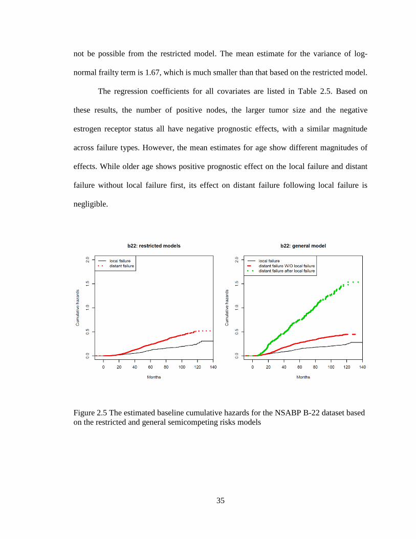
We next fitted a general model with the shared random log-normal intercept using
the same covariates as the restricted model. The estimated baseline cumulative hazards
are shown in Figure 2.5, which also includes the baseline cumulative hazards estimates
based on the restricted model for comparison. We note that the estimated baseline
cumulative hazards for the distant failure after the local failure are the largest from the
general model. It appears that patients who experienced the local failure first would
develop the distant failure much sooner than patients who have the same baseline
covariates but have not yet experienced local-regional failures. This finding is consistent
with the report based on data pooled from five NSABP node-positive protocols (B-15, B-
16, B-18, B-22, and B-25) by Wapnir et. al.[60], which demonstrated that local/regional
failure is associated with increased risk of distant disease and death. Such findings would
Page 49
35
not be possible from the restricted model. The mean estimate for the variance of log-
normal frailty term is 1.67, which is much smaller than that based on the restricted model.
The regression coefficients for all covariates are listed in Table 2.5. Based on
these results, the number of positive nodes, the larger tumor size and the negative
estrogen receptor status all have negative prognostic effects, with a similar magnitude
across failure types. However, the mean estimates for age show different magnitudes of
effects. While older age shows positive prognostic effect on the local failure and distant
failure without local failure first, its effect on distant failure following local failure is
negligible.
Figure 2.5 The estimated baseline cumulative hazards for the NSABP B-22 dataset based
on the restricted and general semicompeting risks models
Page 50
36
36
Table 2.5 NSABP B-22 data analysis using general models ______________________________________________________________________________________________________
Distant occurrence Distant occurrence
Local occurrence without local occurrence after local occurrence
_________________________ ___________________________ _____________________________
Covariate Mean SE 95%CI Mean SE 95%CI Mean SE 95%CI
______________________________________________________________________________________________________
Fixed effect
ER status -0.390 0.142 (-0.669,-0.107) -0.353 0.122 (-0.600,-0.105) -0.334 0.230 (-0.782, 0.087)
nPNodes 1.835 0.249 ( 1.365, 2.329) 1.738 0.208 ( 1.374, 2.149) 1.639 0.384 ( 0.931, 2.397)
nPNodes SQ -0.603 0.143 (-0.895,-0.324) -0.433 0.108 (-0.650,-0.234) -0.638 0.219 (-1.097,-0.221)
Tumor size 0.105 0.041 ( 0.023, 0.184) 0.125 0.033 ( 0.064, 0.193) 0.105 0.057 (-0.009, 0.215)
Age -0.345 0.068 (-0.483,-0.213) -0.302 0.054 (-0.407,-0.203) 0.047 0.100 (-0.149, 0.237)
Random effect variance
Intercept 1.582 0.520 0.795 2.769
________________________________________________________________________________________________________
Page 51
37
2.7 Discussion
We developed flexible frailty models for semicompeting risks data. Our models can
incorporate different covariates into the frailty terms for three different types of hazard
functions corresponding to the illness, death without illness, and death after illness. Our
methods extended the gamma frailty models by Xu et al. (2010) which used a single
frailty term to correlate the events and did not consider covariates for the frailty term. In
clinical trial settings, this model will help address important questions such as whether
continuing treatment is still beneficial for the terminal event after the occurrence of the
non-terminal event. We used Bayesian methods for estimation. Our choice over the EM
algorithm was mainly computational. With the development of general purpose software
packages such as WinBUGS, JAGS and Stan, implementation of the Bayesian approach
and model based predictions became very straightforward.
Our models also will work with clustered data [23, 42]. Further they can be
extended beyond shared frailty models. For example, Gustafson (1997) described a
semicompeting risks model where relapse and death have correlated frailties associated
with clusters in addition to the random intercept specific to individual subjects. Our
model could also be easily extended to such correlated frailty models. We are also
adapting our approach to the joint modelling of semicompeting risks, which will be
presented in Chapter 3.
Page 52
38
CHAPTER 3. JOINT MODELING OF LONGITUDINAL AND SEMICOMPETING
RISKS DATA
3.1 Summary
In medical research, multiple duration outcomes are often recorded along with
longitudinal biomarker measurements. In this chapter, we consider semicompeting risks
duration data that arise when two types of events, non-terminal and terminal, are
observed. When the terminal event occurs first, it censors the non-terminal event, but not
vice versa. For the longitudinal data, we consider repeated continuous measures that may
exhibit nonlinear patterns and can be important predictors for both types of the duration
outcomes. Joint models of the repeated measures and semicompeting risks data provide
most efficient use of data to infer the covariate effects and reduce bias due to the
intermittent observation of the longitudinal biomarker and with the dependent censoring
issue (of the non-terminal event) by the terminal event. In addition, such models also
facilitate an individualized approach for prediction of patient outcome that improves on
simplified models. The method is demonstrated via a simulation study and an analysis of
a prostate cancer study.
Page 53
39
3.2 Introduction
Many biomedical studies collect data on repeatedly measured markers such as CD4 cell
counts for human immunodeficiency virus (HIV) patients, and time-to-event outcomes
such as time to disease progression and time to death. The longitudinal data can be
important predictors or surrogates of the time-to-event outcomes. To describe the
relationship between the longitudinal data and the time-to-event outcomes, joint models
can be very useful. That is, a model is specified for the longitudinal data and then derived
components of the longitudinal model are linked to survival models. The modeling of the
longitudinal data is usually necessary due to the intermittent observations and
measurement error. Nice overviews of this field were given by [61, 62] [44, 63].
In this chapter we consider joint modeling of longitudinal data and semicompeting
risks data. Semicompeting risks data arise when two types of events, a non-terminal event
(e.g., tumor progression) and a terminal event (e.g., death) are observed. When the
terminal event occurs first, it censors the non-terminal event. Otherwise the terminal
event can still be observed when the non-terminal event occurs first [1, 2]. This is in
contrast to the well-known competing risks setting where occurrence of either of the two
events precludes observation of the other (effectively censoring the failure times) so that
only the first-occurring event is observable. More information about the event times are
therefore contained in semicompeting risks data than typical competing risks data due to
the possibility of continued observation of the terminal event after the non-terminal event.
Consequently, this allows modeling of the correlation between the non-terminal and
terminal events without making strong assumptions. Adequate modeling of the
correlation is important to address the issue of dependent censoring of the non-terminal
Page 54
40
event by the terminal event [2-4, 12]. It also can allow modeling of the influence of the
non-terminal event on the hazard of the terminal event and thus improve on predicting the
terminal event [5].
The development of our proposed model was primarily motivated by studies of
prostate cancer, the most commonly diagnosed cancer among American men. In current
practice, patients diagnosed with clinically localized prostate cancer often undergo
radiation therapy or radical prostatectomy, sometimes in combination with hormone
therapies [64]. After initial treatments, patients are actively monitored for prostate-
specific antigen (PSA), a biomarker associated with clinical recurrence of prostate cancer
[65]. Patients with elevated and/or rising levels of PSA sometimes receive additional new
treatment (called salvage therapy) in order to prevent or delay recurrence. One such
salvage therapy is androgen deprivation therapy (SADT), which consists of either
surgical or medical castration. Although SADT is generally thought to be beneficial in
delaying recurrence, the magnitude of the benefit of SADT is not well quantified [66-68].
The benefit of early versus deferred androgen suppression as well as the association of
the effect of SADT with the current health status of the patient (e.g., the current value or
slope of PSA) or other patient characteristics (e.g., age) are not well understood.
One of the complications in determining the effect of SADT is the adapted
treatment decision, which is not predetermined by the investigator, but rather than based
on the current condition of the patient. That is SADT is a “treatment by indication”
which is related to elevated PSA, or rising PSA slope, both being considered as
intermediate variables for the recurrence of prostate cancer. The effect of SADT on the
risk of recurrence of prostate cancer could not be adequately addressed by standard Cox
Page 55
41
regression models. Recently, Kennedy et al. [69] described a two-stage method (and as
well a sequential stratification method) to analyze the treatment effect. However, because
the two-stage method does not appropriately propagate the uncertainty from the analysis
of the first stage, the standard errors may be underestimated.
The basic joint models formulated by Faucett and Thomas (1996) [70]and Wulfson
and Tsiatis (1997)[71] have been extended in multiple ways to accommodate multivariate
survival outcome. These include competing risks data [72-74] [75-77]and recurrent event
data with informative terminal event[78, 79]. Unfortunately, despite the recent rapid
advance on semicompeting risks data, the joint modeling of such data and longitudinal
data has not been explicitly described in the literature. Most of the proposed models on
joint models with multivariate survival outcomes adopted shared frailty models.
Conceivably, the current shared frailty models developed for joint modeling on
multivariate survival data can be utilized for joint models with semicompeting risks data.
However current shared frailty models have the following shortcomings for modeling
semicompeting risks data. First conditioning the frailty terms, the frailty models specify
the joint distribution of the non-terminal event and terminal event in completely
independent manner. However because there is no possibility of observing a non-terminal
event after a terminal event, the shared frailty models are in essence over-specified [18].
In addition, the shared frailty models do not differentiate hazards of the terminal event
before or after the onset of the non-terminal event, and consequently the two type of
events can only be related via a shared frailty term, which may or may not be a sensible
assumption in reality since the onset of the non-terminal event may cause the terminal
event to occur sooner if it is harmful or later if it is a cure. In contrast, our adopted
Page 56
42
‘general model’ assumes that the terminal event ha ard function is possibly changed after
experiencing the non-terminal event on top of the frailty terms. This can have
implications in prediction.
On the other hand, the illness-death models proposed by Xu et al. [18] can
overcome these two shortcomings. However the current approaches do not incorporate
flexible random effects. Such incorporation can provide adequate modeling for complex
observational studies where over-dispersion and outcome heterogeneity are common. In
this chapter, we propose such random effects multistate models to jointly model
longitudinal and semicompeting risks data. For prostate cancer studies, we consider
SADT as the intermediate event and cancer recurrence as the terminating event. We
adopt the illness-death model for semicompeting risks data [18], which allows
specification of three types of baseline hazards and corresponding regression coefficients
associated with two type of events, i.e., the hazard for time to SADT, the hazard for time
to recurrence without SADT and the hazard for time to recurrence following SADT.
Further, we adopt joint modeling approach to appropriately adjust time-dependent PSA
value and its slope when estimating the effect of SADT. The linear mixed model is used
to predict the current value and slope of PSA in the absence of SADT. Although the
observed PSA of patients who received SADT experienced considerable decreases, the
‘latent PSA process’ represents health status that is unaffected by initiation of SADT [69].
The predicted PSA and slope of PSA are incorporated as time-dependent covariates in
proportional hazards models. Based on this joint modeling framework, the effect of
SADT on an individual can then be addressed by comparing the hazards overtime with or
without SADT. Although motivated by the prostate cancer study, the methods described
Page 57
43
here should be generally applicable to studies where both longitudinal and
semicompeting risks data are collected.
Besides parameter estimation, we also focus on subject specific predictions for the
time-to-event outcomes, in particular for the terminal event which can be of most clinical
relevance. Prediction in joint modeling framework has been considered in [80-83]. We
show in this article that in presence of both non-terminal and terminal event, adequate
modeling of longitudinal data and both events are necessary when the prediction of the
terminal event is of main interest.
Computation for such complex models can be challenging. Therefore we adopt
Bayesian MCMC to directly work with the full likelihood. The Bayesian paradigm
provides a unified framework for carrying out estimation and predictive inferences. In
particular, we carry out the computation using an existing software package Stan [35].
The remaining of the chapter is organized as follows. In Section 3.3, we introduce the
details of the joint model, the implementation of a Bayesian approach as well as
individualized prediction of survival outcome. In section 3.4, we present results from a
simulation study. In Section 3.5, we conduct a thorough analysis of the prostate cancer
studies. Section 3.6 contains a brief discussion.
3.3 Model specification
3.3.1 Joint models and assumptions
The proposed joint models consist of two submodels, the longitudinal data
submodel for the observed repeated biomarker measures and the survival submodel for
semicompeting risks data. For notational simplicity, we describe our models using a
simple linear mixed effect model for the marker process. However, more complex models
Page 58
44
such as nonlinear mixed models, B-spline models [48, 84] can be adopted when
necessary. The use of the nonlinear mixed models will be illustrated through our case
study in Section 3.5.
3.3.2 Longitudinal data submodels
Consider a set of subjects. For subject , let denote the unobserved true
values for the biomarker process at time and be the corresponding observed
biomarker process at time . Let and
denote the true and observed marker history up to time . There are a total of
longitudinal observations for subject at observation times . We further
denote ) as the vector of the observed marker values.
The observed and the latent process for subject at are assumed to
satisfy
(3.1) ( )
where are mutually independent for . The latent process
is typically specified as a linear function of time and baseline covariate vector , given
by
(3.2) ( )
The quantities and are taken to be random and have a multivariate normal
distribution,
where denote the mean vector and the covariance matrix.
Page 59
45
3.3.3 Semicompeting risk data submodels
We adopt the same notations and illness-death model for the semicompeting risks
data that is presented in Section 2.3 in Chapter 2. For self-containedness of this chapter,
we repeat it here. For semicompeting risks data, let be the time to the non-terminal
event, e.g., disease progression (referred to as illness hereafter), be the time to the
terminal event (referred as death hereafter), and be the time to the censoring event (e.g.,
the end of a study or last follow-up assessment status). Observed variables consist of
, , , and . Note that
can censor but not vice visa, whereas can censor both and . For subject , we
observe , , .
Semicompeting risks data have been popularly modeled using copula models,
which consists of two marginal distributions for the two types of events and an
association parameter to accommodate dependence. However, with the copula models, it
is not straightforward to incorporate both fixed and random covariates. Here we extend
the illness-death models recently proposed by Xu et al. [18] for more flexible modeling
of semicompeting risks data. With this model, an individual begin in an initial healthy
state (state 0) from which they may transition to death (state 2) directly or may transit to
an illness state (state 1) first and then to death (state 2) (see Figure 2.1). Three distinct
types of hazard functions, denoted by , are differentiated and defined as
follows,
(3.3)
Page 60
46
(3.4)
(3.5)
where . In general, can depend on both and . These equations
define a semi-Markov model. When , the model becomes Markov.
The ratio partly explains the dependence between and . When this
ratio is 1, the occurrence of has no effect on the hazard of . Borrowing the
terminology from Xu et al. [18], we refer models that force as
“restricted models” and models without this assumption as “general” models.
The longitudinal and semicompeting risks components can be linked through
functionals of the latent process , which account for the association of the two types
of outcomes. For notational simplicity, we assume that only the current value
affects the hazard functions. In our data analysis, we have both and its derivative
in the model. In addition, for semicompeting risks data, there may be additional
frailties or random effects . The proportional hazards models are thus given as,
(3.6)
,
where are the baseline functions. Baseline covariates and may overlap
among each other and may overlap with in the longitudinal model too. The random
effects follow a multivariate normal distribution with mean of zero and covariance
matrix , that is, . Note that under the restricted models, the occurrence of
does not alter the baseline hazard function of , that is , then we can
express the hazard models as
(3.7)
Page 61
47
This is the commonly used shared frailty model.
3.3.4 Baseline hazards
Parametric models such as the exponential, Weibull, gamma, and lognormal models can
be used for baseline hazards. Nonparametric models similar to the Cox proportional
hazards models [85] can also be used. Alternatively one can also use parametric but
flexible models such as piecewise-constant (PWC) models [86] [38] and regression
splines [48].
In a Weibull model, . The proportional hazards model is
given as,
(3.8)
The baseline hazards is monotone in If , the Weibull model is reduced to
the exponential model with the constant hazard.
In a PWC model, for , the follow-up times are divided into intervals
with break points at where equals or exceeds the largest observed
times and . Usually is located at th quantiles of the observed failure times.
The baseline hazard function then takes values in the interval ] for
, that is, . Obviously when the number of
break points increases, the baseline hazards become more flexible. In the limiting case
where each interval contains only a single true event time (assuming no ties), this model
is equivalent to the Cox model where the baseline hazards are left unspecified.
Although Cox models are widely used for survival analysis, the use of this method
for the joint modeling meets with some computational challenge. Due to the inclusion of
Page 62
48
random effects into the hazards, an EM algorithm based on profile likelihood approach is
typically used for estimation of standard errors of the maximum likelihood estimates
(MLEs). However, this method would lead to underestimation of standard errors of EM
estimators [87] [88]. Bootstrapping is therefore proposed for estimation of standard errors.
However, it is evident that computation load is rather demanding. With Bayesian
methods, on the other hand, because the inference on hazard parameters is based on exact
posterior distributions, it is feasible to fit joint models with Cox proportional hazards.
Nevertheless, the computation load also tremendously increases when the number of
distinct events increases.
3.3.5 Joint likelihood
To derive the joint likelihood, we adopted counting process notations for survival
data. Let , , and
be the counting processes for the three patterns of
the event process. Correspondingly, let
and be the at-risk process for the three patterns of events.
Denote as the event indicator associated with each type of hazard, as the
corresponding observed times. Hence, , ; , ;
, .
With the proportional hazards assumptions and the non-informative censoring
assumption for , the joint likelihood for subject , is given as,
(3.9)
Page 63
49
∏ ( | )
∏[∏
{ ∫
}]
where
. In particular, the joint
likelihood under the PWC baseline hazard can written as,
(3.10)
∏ ( | )
∏[
]
[
∑ ∫
]
where are at risk functions that equals to 1 if the subject is at risk for hazard type
In particular, for , for and 0 otherwise. For ,
only when =1 and .
Since the random effects and are not observed, the standard likelihood
approach to this problem involves integration of the joint likelihood over the distribution
of random effects. In addition, there is also an integral with respect to time for the
survival function that incorporates time-dependent marker values. Since the integrations
may not have close-form solutions, numerical solutions can be employed to approximate
these integrals. However approximations may not work well due to the nonlinear nature
of the integrands, especially when the dimensionality of random effects is not small.
Therefore programming becomes very demanding and can require problem-specific fine
tuning for stable numerical results. The Expectation-Maximization (EM) algorithm is
Page 64
50
commonly applied to joint modeling [62, 71, 89]. However these computational
challenges remain.
3.3.6 Bayesian approach and prior specification
We utilize Bayesian MCMC approach for parameter estimations [70, 90-92]. The
Bayesian computation can be conveniently implemented in standard Bayesian software
like WinBUGS [51], JAGS[34] and Stan [35]. In addition, posterior draws of all
parameters, including random effects, are stored, which facilitates easy approximation of
integrals. Consequently individual predictions can be done quickly.
For Bayesian analysis, prior distributions need to be specified for all parameters.
When there are no prior data, non-informative or diffuse prior distributions can be
specified. In general, the prior distributions can be chosen to be proper and conjugate to
the likelihood while remain fairly non-informative. For regression coefficients,
we will assume normal prior distributions with means of zero
and large variances (e.g., 10,000). For , we will assume an inverse gamma distribution
with shape and scale of 0.01. For , we will assume inverse-Wishart prior
distribution , where d is the rank of , which is the smallest possible value for
this distribution. The scale matrix is often chosen to be an identity matrix multiplied by
a scalar, . The choice of should ensure that the prior distribution can leave
considerable prior probabilities for extreme values of the variances terms. For parameters
of baseline hazards , and , gamma priors are specified with shape and scale of 0.01.
For the scale parameter of Weibull distribution, a normal prior is assumed on its
logarithm.
Page 65
51
All simulations and data analysis are done using Stan, which is a new piece of
software that allows a very flexible way of specifying the likelihood and obtaining
Bayesian inference [35]. Stan utilizes the No-U-Turn sampler, a variant of Hamiltonian
Monte Carlo (HMC), which takes a series of steps informed by the first-order gradient
information of logarithm of posterior distribution and hence avoids the random walk
behavior of simpler MCMC methods. These features allow it to converge to high-
dimensional target distributions much more quickly [93]. In our experience, Stan has
significant computational speed advantage over WinBUGS and JAGS with our proposed
joint models.
3.3.7 Prediction of Survival Probabilities
The joint model enables the prediction of patient survival outcomes using all
available information, including both the baseline information and highly individual
longitudinal biomarker levels. There have indeed been many related works [80-83]. With
semicompeting risks data, information from the non-terminal event should in general be
utilized to provide valid prediction of the terminal event. Such necessity arises first from
the fact that the transition rate to the terminal event can greatly differ before and after the
non-terminal event. Secondly, quite often the longitudinal biomarker is not measured
after the non-terminal event, the non-terminal event therefore represents an important
aspect for prediction of the terminal event, especially when the non-terminal event
happens early.
Specifically, we are interested in predicting survival probabilities for the subject ,
who has survived the terminal event up to time and has a set of longitudinal
measurements ). In this context, it is more relevant to calculate
Page 66
52
conditional probability of surviving time given the survival up to . If the
subject has experienced non-terminal event, the conditional survival probability for the
terminal event is,
(3.11)
When the subject is censored for both nonterminal and terminal events, the
conditional survival probability can be calculated as below,
(3.12)
where
∫
Posterior distributions of these conditional survival probabilities can be obtained easily
by substituting the stored posterior samples for and all other parameters such
as the baseline hazards.
3.4 Simulation studies
Simulation studies were performed to examine the feasibility and properties of the
proposed joint models. The simulated datasets included repeated measurements and
semicompeting risks data. The simulations consisted of 400 replications, each composed
Page 67
53
of subjects. Eight visits are scheduled at equally spaced time points between 0
and 4 months. The measurements of the longitudinal variable became missing after
, that is when subjects experienced the non-terminal event or censored
from studies. For simplicity, we set months. In addition to parameter estimation
for various parts of the joint model, we investigated terminal event prediction based on
various models. Specifically, we fit five joint models: three general models based on (3.6)
that used Weibull, 10-piece PWC, and nonparametric baseline hazards respectively; the
restricted model based on (3.7), and the joint model based on univariate survival
submodel that used only the terminal event but ignored the non-terminal event.
For simplicity, the longitudinal submodel (3.2) used in our simulation was a linear
mixed model consisting of random intercept and slope with mean
and variance =
with
and
. We also
include a single binary covariate with its covariate effect The residual of
measurement errors follows normal distribution with a mean of zero and .
For semicompeting risks data, we specified Weibull distributions for the baseline
hazards, i.e. with and for , 2, and 3. The
proportional hazards model (3.8) includes the single baseline covariate and the current
value of the true longitudinal variable value . Corresponding parameters for and
the current value in the survival submodels are , and
for the three hazard functions respectively. Because
affects the hazard functions not only through but also affect through , we also
Page 68
54
consider in our results comparison among various models we fit. These
derived quantities in some sense gauge the total effects of on the hazard functions.
For Bayesian analysis, flat priors specified in Section 3.3.6 were used for all
parameters except when fitting joint models based on Weibull baseline hazards. In that
case, we used slightly informative prior distributions to speed up convergence of MCMC
chains. A uniform prior on support of (-6, 0) is assumed on and a gamma prior is
specified with both shape and scale of 0.1 for . Integrations over time was
approximated by 16-points Gaussian quadrature. The computation was performed in
Linux clusters with over 1000 CPU processors (2.60GHz Intel Xeon CPU E5-2670 with
16 GB memory). Each data analysis was done using three MCMC chains with a burn-in
period of 1,000. Algorithm convergence was monitored using the method of Gelman-
Rubin [57]. Posterior distributions of parameters were summarized from 1,000 iterations.
For joint models based on general semicompeting risks survival submodels, it took an
average of 3.50 and 8.95 minutes when using the 10-piece PWC baseline hazard
functions and the Weibull baseline hazard functions, respectively. For Cox models, it
took an average of 24.3 hours due to the large number of parameters resulted from the
nonparametric baseline hazards. The computing time reduced drastically to 2.67 on
average when we fit datasets with 200 subjects. In a typical simulated data set with 600
subjects, there are typically 2170 longitudinal observations, 280 non-terminal events and
370 terminal events (278 without first experiencing the non-terminal events and and 67
after the non-terminal ones). Therefore, for the Cox models, the computation load
significantly increases as the sample sizes grow.
Page 69
55
3.4.1 Results for simulation
For parameter estimations, we report in Table 3.1 the average biases (Bias), the standard
deviation of the mean estimates (SD) and the coverage probabilities (CP) based on 95%
the credible intervals. When the joint model based on univariate survival submodel was
fit, large biases were observed for all parameters especially for the survival parameters,
leading to poor coverage probabilities from the 95% credence intervals. The biases are
relatively smaller from the joint model based on restricted semicompeting risks models.
The parameter estimates for longitudinal model all improved. For the survival outcomes,
the estimates for the parameters and that are associated with the non-terminal
event are all well estimated. However, for the terminal event, both and are
underestimated while both and are over-estimated. In contrast, all parameters are
well estimated when joint models based on (3.6) were used to fit the data sets, for all
three different baseline models: Weibull, 10-piece PWC and Cox models. The biases are
all small and coverage probabilities are all close to 95%.
Page 70
56
Table 3.1 Parameter estimation for simulation studies based on various joint models __________________________________________________________________________________________________________
Univariate Restricted General General General
Weibull Weibull Weibull PWC Cox
_________________ _________________ _________________ ________________ __________________
Par Truth Bias SD CP(%) Bias SD CP(%) Bias SD CP(%) Bias SD CP(%) Bias SD CP(%)
__________________________________________________________________________________________________________
Longitudinal submodel parameters
0.4 0.029 0.035 87.4 0.015 0.036 92.6 0.002 0.036 94.0 0.002 0.036 94.5 -0.001 0.036 94.4
0.5 -0.097 0.018 0 -0.049 0.019 32.0 -0.001 0.021 92.8 -0.002 0.021 95.0 -0.004 0.021 93.3
0.4 -0.028 0.048 90.9 -0.016 0.049 92.9 -0.003 0.049 94.5 -0.004 0.049 95.3 -0.001 0.049 94.9
0.5 -0.020 0.021 82.5 -0.010 0.021 91.4 0.001 0.021 94.5 -0.002 0.022 93.0 0.001 0.022 94.0
0.2 -0.030 0.018 65.9 -0.015 0.018 87.2 -0.003 0.018 95.3 -0.004 0.018 94.8 -0.004 0.018 95.4
0.5 0.007 0.010 88.3 0.003 0.010 91.9 0.001 0.010 95.3 0.001 0.010 94.0 0.001 0.010 94.6
Survival submodel parameters
0.2 0.005 0.134 93.8 0.010 0.133 91.8 0.002 0.136 94.8 -0.008 0.135 93.9
0.2 0.089 0.115 86.7 0.171 0.115 67.2 0.007 0.133 94.8 0.004 0.135 93.8 -0.006 0.134 94.9
0.8 -0.511 0.115 0.5 -0.429 0.115 03.2 0.064 0.295 94.0 0.042 0.299 95.3 0.008 0.297 94.9
1.5 -0.011 0.170 92.1 0.038 0.170 92.8 0.045 0.177 95.0 -0.027 0.167 94.1
1.5 -1.104 0.114 0 -1.367 0.100 0 0.031 0.170 95.3 0.030 0.176 95.8 -0.069 0.167 91.3
0.2 0.196 0.114 57.9 -0.067 0.100 86.9 -0.089 0.282 95.3 0.024 0.298 96.5 0.028 0.287 94.9
Total effect of binary covariate on survival
0.8 0.023 0.147 94.8 -0.021 0.149 94.8 -0.015 0.150 96.3 0.021 0.147 95.6
0.8 0.363 0.111 10.3 0.378 0.109 6.9 -0.014 0.150 94.8 -0.011 0.150 94.8 0.035 0.146 94.6
0.88 0.443 0.111 03.0 0.458 0.109 1.7 -0.028 0.288 94.0 -0.052 0.293 94.8 -0.020 0.288 94.6
Weibull baseline parameters
ln -3.22 0.006 0.220 95.6 0.056 0.224 94.3
ln -3.22 1.054 0.139 0 1.249 0.128 0 0.058 0.223 95.3
ln -3.22 1.054 0.139 0 1.249 0.128 0 0.088 0.603 96.5
1.05 0.003 0.072 93.6 -0.003 0.071 92.3
1.05 -0.092 0.064 70.8 -0.006 0.067 94.6 0.007 0.071 95.8
1.05 -0.092 0.064 70.8 -0.006 0.067 94.6 0.162 0.347 96.5
__________________________________________________________________________________________________________
Page 71
57
We next evaluated the performance of each model for the terminal event prediction
for censored patients at 4.5, 5.25, 6, 6.75 and 7.5 month. We calculated the survival
probabilities for the terminal events at these time points, conditional on the event history
and longitudinal profile. The sums of the event probabilities among these censored
patients were taken as estimates for the predicted total numbers of events that may occur
between 4 month and the corresponding future time points. These estimates were then
compared with observed numbers of events accordingly. In Table 3.2, we list prediction
results from the joint model based on univariate survival submodel, the joint model based
on restricted model, the joint model using Weibull baseline hazards, and the true model.
We see that the general model predicted the number of events quite comparable to that
based on true parameter values, both are close to the observed number of events. In
contrast, both the restricted model and univariate terminal event joint models over
predicted the number of events.
Table 3.2 Event prediction based on different joint models _______________________________________________________________________
Univariate Restricted General True
Observed model model model parameter
___________ _____________ _____________ ___________ ____________
Time Average SD Average SD Average SD Average SD Average SD
_______________________________________________________________________
4.5 19.8 4.3 33.2 1.8 30.3 2.1 22.1 2.5 21.4 1.7
5.25 45.3 6.2 77.7 4.2 70.2 4.9 50.2 6.5 48.1 3.2
6 67.0 7.6 115.9 6.1 104.1 7.3 74.0 10.8 70.8 4.3
6.75 86.9 8.6 147.9 7.5 132.6 9.3 94.7 15.3 91.0 5.3
7.5 105.2 9.5 173.9 8.2 156.2 10.6 112.9 19.7 109.3 6.1
_______________________________________________________________________
In Figure 3.1, we also plotted predicted survival probabilities for the terminal
event from the general Weibull baseline hazards and the restricted models for two
selected subjects. Subject 22 experienced the non-terminal event at 1.8 month and then
Page 72
58
got censored at 4 month. The predicted survival probabilities at 7.5 month are 0.75 and
0.42, respectively (see the top panel of Figure 3.1). Subject 38 was censored at 4 month
for both the non-terminal and terminal events. The predicted curve from the general
Weibull baseline hazards model took into account two possible path of terminal event.
For one path, the terminal event occurs before non-terminal event. For the other one, the
terminal event occurs after the non-terminal event and the occurrence of the non-terminal
event changes the hazard function over time. This is in contrast with the restricted model.
The predicted survival curve has quite a different shape (see bottom panel of Figure 3.1).
Figure 3.1 Predicted survival probabilities for two simulated subjects based on general
and restricted models.
Page 73
59
3.5 Application to prostate cancer studies
The analysis dataset contains 1947 clinically localized prostate cancer patients who
were initially treated with the external beam radiation therapy (EBRT) [94]. Patients
came from the University of Michigan and the William Beaumont Hospital in Detroit.
Patients were monitored for PSA periodically throughout follow-up. We plotted the log-
transformed longitudinal PSA profiles for a sample of 50 patients in the left panel of
Figure 3.2. Generally, the values decline initially and then increase. From
the right panel of Figure 3.2, patients that received SADT appear to have higher
recurrence free probabilities than those that did not.
Figure 3.2. Individual PSA profiles from randomly selected 50 patients (left) and Kaplan-
Meier curve on recurrence (right).
A summary of the data are listed in Table 3.3. The median number of PSA
measurements prior to the SADT is 8 times per patient. There were 11.8% patients who
received SADT. Among 287 cases of recurrence, 45 were treated with SADT and 242
Page 74
60
were untreated. The median time to clinical recurrence is 6.5 years for patients treated
with SADT and 3.7 years for those untreated. The median time to SADT is 4.4 years.
Table 3.3 Description of PSA data
_________________________________________________________
Item Category Summary
_________________________________________________________
Paitents (#) 1947
PSA measures (#) 17796
Age (years) 72.0(58.0,81.0)
Pretherapy PSA (ng/ml) 7.9( 2.3,41.0)
Clinical T-stage(#) 1 626( 32.2%)
2 1210(62.1%)
3-4 111( 5.7%)
Gleason score(#) 2-6 1249(64.1%)
7 518(26.6%)
8-10 180( 9.2%)
PSA measures/patient 8.0(3.0,19.0)
SADT 230(11.8%)
Time to SADT(years) 4.4(1.4,8.5)
Clinical recurrence Without prior ADT 242(12.4%)
With prior ADT 45( 2.3%)
Total 287(14.7%)
Time to clinical
recurrence (years) Without prior ADT 3.7(1.3, 8.6)
With prior ADT 6.5(1.8,10.6)
Time to last
contact (years) 4.9(1.5,10.9)
_________________________________________________________
The underlying curve for the longitudinal data, takes the following
form [69]:
(3.13)
( ) ( )
where and are used to capture the short term and long-
term evolutions respectively; are baseline covariates;
Page 75
61
are fixed effects and are random effects. Note that the timing of the
SADT can be viewed as a random variable that is associated with baseline characteristics
and disease progression status of patients. We therefore consider the time to SADT as the
non-terminal event and cancer recurrence as the terminal event. The corresponding
proportional hazards models is given,
(3.14)
( )
where is the derivative of representing the slope of the log-transformed
PSA process and are baseline covariates. We use patient age, baseline prostate
specific antigen (bPSA), Tumor stage (T-stage), and Gleason score as covariates in both
(3.13) and (3.14). The T-stage was dichotomized and takes a value of 1 when the actual
tumor stage is 1 and 0 otherwise. The other three covariates are continuous and mean-
centered. The baseline hazards are modeling using PWC functions with 8 pieces in the
analysis. Bayesian MCMC method is used to fit the models with non-informative prior
specified for all parameters. The complete Stan code is given in the Appendix C. The
trace plot of MCMC chains and density plots for several regression parameters are shown
in Figure 3.3. The MCMC chains for all parameters have reached their stationary
posterior distribution and are mixing very well.
Page 76
62
(Age on survival submodel)
(Current PSA value on survival submodel)
(Baseline hazard of 1
st interval for time to SADT)
(Residual error of longitudinal submodel)
Figure 3.3 Posterior marginals for selected parameters.
The left column gives superimposed time-series plots of the three Markov chains. The
right column gives posterior marginal distribution density for the corresponding
parameters.
3.5.1 Analysis results for the prostate cancer study
The analysis results on the prostate cancer study based on the joint models are
listed in Table 3.4 for the PSA longitudinal submodel and Table 3.5 for the survival
submodel. It is observed that for the phase 0 part of (3.13), the 95%
credible intervals of all covariates exclude zero, indicating significant fixed effects. For
Page 77
63
the phase 1 part, , that is related to , and for the phase 2,
, that is related to , the effect of age is negligible. On the other hand, higher
Gleason score, later T-stage, and higher baseline PSA are all positively correlated with
the magnitude of the slopes for both phase 1 and 2.
Table 3.4 Analysis results for the longitudinal submodels on PSA _______________________________________________
_______________________________________________
Covariate Mean SE 95%CI
________________________________________________
Phase 0
Intercept -1.165 0.036 (-1.240,-1.090)
Gleason -0.143 0.026 (-0.196,-0.092)
T_stage 0.369 0.068 ( 0.236, 0.498)
Age -0.013 0.004 (-0.022,-0.005)
bpsa 0.095 0.037 ( 0.023, 0.168)
Phase 1
Intercept 2.743 0.044 ( 2.654, 2.827)
Gleason 0.125 0.032 ( 0.063, 0.186)
T_stage -0.490 0.081 (-0.647,-0.328)
Age 0.006 0.005 (-0.005, 0.017)
bpsa 0.746 0.045 ( 0.657, 0.831)
Phase 2
Intercept 0.404 0.016 ( 0.373, 0.433)
Gleason 0.062 0.011 ( 0.039, 0.083)
T_stage -0.213 0.029 (-0.268,-0.155)
Age -0.003 0.002 (-0.007, 0.001)
bpsa 0.229 0.016 ( 0.199, 0.261)
Covariance
1.330 0.060 ( 1.218, 1.448)
1.643 0.084 ( 1.482, 1.810)
0.253 0.013 ( 0.229, 0.279)
-0.868 0.008 (-0.882,-0.852)
-0.517 0.022 (-0.558,-0.473)
0.510 0.023 ( 0.462, 0.555)
Residual
0.288 0.002 ( 0.284, 0.291)
__________________________________________________
Page 78
64
For the random effects, all variances for the three phases have 95% credible
intervals excluding zeros, demonstrating substantial heterogeneity for PSA trajectories.
There is also a large negative correlation between the random effects for phase 0 and
phase 1, suggesting a sharper PSA drop for higher baseline PSA subjects. Modest
correlations also exist between phase 0 and phase 2 random effects and between phase 1
and phase 2 random effects.
The piecewise baseline hazards based on the joint models are shown in Figure 3.4.
It appears that the baseline propensity of receiving SADT is similar to the baseline hazard
of cancer recurrence without SADT. On the other hand, the baseline hazards of
recurrence are much higher for SADT treated patients during the first five years of
follow-up. In fact, among 58 patients who received SADT within the period of (0, 2.79),
6 experienced recurrence during this period and 13 more experienced recurrence later.
The initial surge of the hazards may reflect the fact that SADT may not benefit those sick
patients with imminent recurrence.
In Table 3.5, we see that the estimates for T-stage, both PSA current value and
slope are all significant for the propensity of receiving SADT. In particular, the PSA
slope has a very large effect. Older age and higher Gleason score are associated with
higher hazards for recurrence when no SADT are received, but their association became
insignificant after SADT. The effects of T-stage, however, are significant regardless of
the SADT. Both PSA slope and PSA current value are strong predictors of cancer
recurrence for those patients receiving no SADT. On the other hand, both have negligible
effects on cancer recurrence after SADT. This demonstrated that the projected PSA
Page 79
65
process will not be a good predictor of recurrence anymore once patients received SADT.
In some sense, disease progression process appears to be substantially altered.
Analysis results from the joint models allow us to dissect the differential
treatment effect of SADT among different subpopulations, defined by covariate values.
In Figure 3.5A, the fitted PSA process for late and early T-stage is plotted. The PSA
values in both groups first decrease and then increase over time. However, the increasing
slopes significantly differ from each other. In Figure 3.5B, the hazard of recurrence over
time for patients with late T-stage was plotted for patients either treated or untreated with
SADT. The hazard of recurrence for patients who did not receive SADT dramatically
increases after year 5. However, the hazards for patients who received SADT remained
relatively flat. Patients of early T-stage also benefits from SADT treatment. However, the
treatment effect is much smaller.
Figure 3.4 Baseline survival based on joint models
Page 80
66
Table 3.5 Survival submodels based on two-stage and simultaneously joint modeling
________________________________________________________________________________________________________
SADT Recurrence without SADT Recurrence after SADT
_________________________ ___________________________ ___________________________
Covariate Mean SE 95%CI Mean SE 95%CI Mean SE 95%CI
______________________________________________________________________________________________________
Baseline covariates
Age -0.002 0.010 (-0.022, 0.018) -0.034 0.009 (-0.052, -0.015) 0.023 0.025 (-0.025, 0.075)
bpsa 0.148 0.084 (-0.019, 0.311) -0.120 0.080 (-0.276, 0.030) -0.263 0.178 (-0.615, 0.077)
Gleason -0.000 0.052 (-0.101, 0.100) 0.170 0.053 ( 0.065, 0.277) 0.028 0.127 (-0.218, 0.283)
T_stage 0.382 0.186 ( 0.020, 0.740) -0.494 0.236 (-0.982, -0.051) -1.515 0.819 (-3.308, -0.126)
Unobserved PSA process
PSA value 0.578 0.069 ( 0.439, 0.712) 0.640 0.064 ( 0.516, 0.762) 0.143 0.085 (-0.024, 0.311)
PSA slope 1.863 0.219 ( 1.437, 2.315) 1.612 0.191 ( 1.248, 1.989) 0.047 0.619 (-1.177, 1.237)
_______________________________________________________________________________________________________
Page 81
67
Figure 3.5 Fitted PSA process and hazard process for early and late T-stage patients.
Page 82
68
3.5.2 Results of prediction for prostate cancer study
To illustrate individualized prediction of cancer recurrence, we consider
prediction curves of cancer recurrence for 3 subjects. Patient 1175 was 86 years old at
baseline with a later T-stage and Gleason score of 7. He received SADT at 4.38 years and
censored for recurrence at 9.37 years. Patient 70 was 54 years old at baseline with a late
T-stage and Gleason score 6. He was censored at 5.8 years for both SADT and recurrence.
At the time of censoring, this patient has a relative low PSA value and a descending slope.
Patient 117 was 70 years old at baseline with a late T-stage and Gleason score 5. Similar
to patient 70, he was censored at 8.16 years for both SADT and recurrence. At the time of
censoring, the patient has a rising PSA slope and a high value of PSA. The prognosis for
patient 70 should be much better than patient 117.
Figure 3.6 Prediction of survival for a patient receiving SADT
Page 83
69
Figure 3.7 Prediction of survival probability for a healthier patient.
For patient 1175, prediction of cancer recurrence is according to and
illustrated in Figure 3.5. For patients 70 and 117 that were censored for both SADT and
recurrence, we can predict the cancer recurrence similar to our simulation study by using
our joint illness-death model that automatically account for the ‘random’ nature of
receiving SADT. However, we can also withhold SADT or give SADT at any time prior
to cancer recurrence and then use the joint illness-death model for prediction. However
these two approaches alter the ‘randomness’ in the SADT and therefore are at the risk of
Page 84
70
extrapolation from the observed data. For example, we can give SADT for a patient with
excellent prognosis in our prediction, but such case may never arise in practice and
therefore no data were available to test the validity of the prediction. Nevertheless, we
still did the predictions in three fashions for our curiosity. In Figure 3.6, we see that the
recurrence probability remain low whether the patients follow the current practice of
receiving SADT (Figure 3.6.A), given SADT at year 5.8 (Figure 3.6.B), or withhold
SADT forever (Figure 3.6.C), Note that the predicted recurrence-free probability for this
patient decreased by about 5% toward the end of year 15 when given SADT at year 5.8,
compared with the current practice of receiving SADT. It seems that SADT does minor
harm to this patient. Again this may be explained by the extrapolation nature of the
prediction when given SADT at year 5.8. The prediction of the survival probability of
this patient with very good prognosis, is based on data observed on SADT treated
patients who were relatively sick and usually expecting imminent recurrence.
Unfortunately, the observed data could not be used to test the validity of such
extrapolation and therefore we cannot rule out the possibility that SADT in fact may do
more harm than good to patients with good prognosis.
The prediction for patient 117 is shown in Figure 3.7. The predicted recurrence
probability is very high if this patient follows the current practice of receiving SADT
(Figure 3.7.A) or withholds SADT (Figure 3.7.C). However, if the patient receives SADT
from the time of censoring (Figure 3.7.B), the recurrence probability of the patient will be
substantially lowered, to about 22% at 15.4 years. This indicates the importance of early
SADT for this patient. Also we caution readers about the possible prediction bias
associated with extrapolation, which in this case may be less severe.
Page 85
71
Figure 3.8 Prediction of survival probability for a sicker patient
3.6 Discussion
We have developed a Bayesian joint modeling framework for longitudinal and
semicompeting risks data. The Bayesian computation can be conveniently performed
using standard Bayesian software including WinBUGS, JAGS and Stan. Although the
EM algorithm can also be developed, programming may become very cumbersome due
to the requirement for integration over multivariate frailty terms. The Bayesian
framework also made individualized event prediction very straightforward. In addition,
Page 86
72
the Bayesian framework described here can be easily extended. Possible extensions
include incorporation of multiple longitudinal markers and using semiparametric models
for longitudinal data [48, 84].
One unique feature of our joint models is the use of illness-death models for survival
outcome. To our knowledge, although this method has been proposed recently by Xu et
al., its use in the framework of joint modeling has not been reported. In the literature,
similar problems were addressed by time-varying covariate approach [69], the joint
models with a bivariate survival models [46], or by competing risks models [77]. The
main advantage of the illness-death model is its flexibility to differentiate two types of
hazards on the terminal event, one occurring after intermediate event and one without it,
thus allowing specifying different baseline models, and incorporating different regression
coefficients. When applied to prostate cancer data, it enables us to dissect and compare
the effect of PSA trajectory and baseline covariates on two separate survival path, one
receiving SADT and one remaining untreated. This model not only allow us to address
the interaction between the SADT and patient health status (PSA profile, T-stage) but
also enable us to predict the patient outcome according to the current practice by
accounting for the probability of receiving SADT.
As with many other models, there is a limitation to statistical inference based on
extrapolations. Obviously, the two patient populations, i.e., treated and untreated by
SADT, may have very different healthy status. We expect to see some bias, for example,
when we attempt to predict the effect of SADT on healthier people. Therefore the
conclusions based on this analysis should to be used with some cautions.
Page 87
73
CHAPTER 4. WEIGHTED RANDOMIZATION TESTS FOR MINIMIZATION WITH
UNBALANCED ALLOCATION
4.1 Summary
Re-randomization test has been considered as a robust alternative to the traditional
population model-based methods for analyzing randomized clinical trials. This is
especially so when the clinical trials are randomized according to minimization which is
a popular covariate-adaptive randomization method for ensuring balance among
prognostic factors. Among various re-randomization tests, fixed-entry-order re-
randomization is advocated as an effective strategy when a temporal trend is suspected.
Yet when the minimization is applied to trials with unequal allocation, fixed-entry-order
re-randomization test is found biased and thus compromised in power. We find that the
bias is due to non-uniform re-allocation probabilities incurred by the re-randomization in
this case. Therefore we propose a weighted fixed-entry-order re-randomization test to
overcome the bias. The performance of the new test was investigated in simulation
studies that mimic the settings of a real clinical trial. The weighted re-randomization test
was found to work well in the scenarios investigated including the presence of a strong
temporal trend.
Page 88
74
4.2 Introduction
Randomization is the foundation of modern controlled clinical trials. It establishes
causality and provides a basis for inference [95]. By ensuring proper balance of
prognostic factors in treatment and control groups, randomization leaves the treatment
under test as the only dissimilarity. Proper randomization can also eliminate or reduce
any conscious or unconscious selection biases in subject allocation. However, in practice
randomization often does not work so ideally, especially for trials of small sample sizes
[96]. For trials with many prognostic factors or confounders, the balance between
treatment groups across the covariates can be achieved by stratified block randomization
[97]. However, the performance of stratified randomization deteriorates as the number of
strata increases, particularly in small trials [98].
In such settings, minimization, a covariate-adaptive randomization procedure, can
be employed. The method of minimization was proposed by Taves [99] and generalized
by Pocock and Simon to clinical trials with equal allocation of subjects for each group
[100]. With this method, subjects are assigned to minimize imbalance among prognostic
factors. That is, for every possible assignment, a pre-specified measure of overall
covariate imbalance will be calculated. A treatment is preferred if inclusion of the new
subject into that treatment group minimizes the overall covariate imbalance. Commonly
used imbalance measures include marginal balance which is obtained by normalizing the
absolute imbalance by subject counts [101] and range. The new subject is then allocated
to the preferred treatment either deterministically, or with a ‘high’ probability of pH that
is larger than 0.5. In case when the assignment of the new subject does not affect the
overall imbalance, the subject is assigned randomly to the treatments. Pocock and
Page 89
75
Simon’s method cannot be applied directly to the case of unequal allocation [95, 101-
104]. Simple modifications of minimization tend to have a smaller allocation ratio than
the desired target. We recently described a biased coin minimization (BCM) that achieves
the desired allocation ratio by varying the probability of assigning the preferred treatment
according to the allocation ratio [105].
Although the majority of the primary analyses for clinical trials are performed
using population-based models that assume independent and identically distributed
random samples, re-randomization or permutation based inference provides an attractive
alternative in case of model assumption violation. Re-randomization test solely relies on
the specific randomization procedure employed in the trials. In particular, a test statistic
is evaluated using both the observed data and the re-randomized data or the reference set.
P-value of the statistic is calculated by comparing the observed test statistic with the
reference set. Simon suggests that, besides the subject responses and covariate values, the
entry order of the subjects should all be fixed during the re-randomization[106]. For
setting of equal allocation, Hasegawa and Tango (2009) conducted Monte Carlo
simulation to compare such fixed-entry-order re-randomization test with the t -test and
the analysis of covariance (ANCOVA) following minimization [107]. They concluded
that the fixed-entry-order re-randomization test is an indispensible alternative. The Food
and Drug Administration (FDA) frequently requests re-randomization tests to confirm the
results from population-model based tests, particularly when a confirmatory clinical trial
was randomized by minimization [97].
For minimization with unequal allocation, however, Proschan, Brittain and
Kammerman discovered serious problems with the fixed-entry-order re-randomization
Page 90
76
test [108]. In a randomized, double-blinded and placebo-controlled trial from Genzyme,
the “Late Onset Treatment study (LOTS)” 90 subjects with late-onset Pompe’s disease
were enrolled and randomized to alglucosidase alfa (60 subjects) or placebo (30 subjects)
[109]. A modified Pocock and Simon minimization algorithm was used to balance three
factors: clinical sites (8-levels), 6 minute walk tests (6MWT) (2 levels: 300m , 300m )
and forced vital capacities (FVC) (2 levels: 55% predicted, 55% predicted). The
actual minimization algorithm can be found in an addendum to the FDA briefing material
at http://www.fda.gov/ohrms/dockets/ac/08/briefing/2008-4389b1-00-FDA-index.htm.
The primary efficacy analysis was performed by the ANCOVA on the change of two co-
primary endpoints from baseline to week 78. The fixed-entry-order re-randomization test
was chosen as the pre-specified sensitivity analysis. At the conclusion of the trial, the p
value for one of the two co-primary endpoints was 0.035 based on ANCOVA, but was
0.06 from the re-randomization test. The discrepancy led to an intriguing discussion
regarding the interpretation of the re-randomization test during an FDA advisory
committee meeting on October 21, 2008 [110]. The fixed-entry-order re-randomization
test distribution was not centered around zero and the validity of re-randomization test
was questioned. It appeared that the re-randomization test broke down with the unequal
allocation minimization, whose use is consequently discouraged [108].
In this chapter, we examine the properties of the fixed-entry-order re-randomization
test in detail, and propose a valid re-randomization test for the unequal allocation
minimization. The performance of various methods will be evaluated through extensive
simulation studies that mimic the LOTS trial. The remaining of the chapter is organized
as follows. In Section 4.3, we briefly review the concept of the re-randomization test and
Page 91
77
then carefully examine the shift in the mean of the fixed-entry-order re-randomization
test distribution with unequal allocation minimization. In Section 4.4, we propose a
weighted fixed-entry-order re-randomization test and a random-entry-order re-
randomization test. In Section 4.5, we evaluate our proposed tests through extensive
simulations. In Section 4.6, we apply the proposed approaches to an example data set that
mimics the motivating example. In Section 4.7, we conclude the chapter with discussions.
4.3 Noncentral distribution of the fixed-entry-order re-randomization test
4.3.1 Notations and the re-randomization test
The most commonly used analysis for clinical trial is based on population models.
That is, for a clinical trial with subjects, the observed subject responses are
considered as realizations of random variables while the actual treatment
assignment, and covariates are considered as fixed. The
treatment indicator if subject is assigned to treatment A and 0 if to B. The
underlying population model is here taken as a linear regression model,
(4.1) ( )
where and are the treatment effects; is a vector of regression coefficients, and
is the variance of the error term. Test of equality between and is based on the
ANCOVA or the -test if is absent.
Re-randomization or permutation tests on the other hand consider the observed
responses and covariates as a set of fixed values. The treatment assignment is then re-
randomized using the same allocation mechanism as the trial. Let be the number of the
re-randomizations performed. Statistical inference or -value is evaluated by comparing
the observed treatment difference with the re-randomized treatment differences.
Page 92
78
Obviously each treatment re-randomization sequence is a realization of the random
binary variables , j=1,…,n}, where if a subject is assigned to treatment A and 0
if to B.
Denote and as the targeted allocation number, and and as
the actual assigned numbers to A and B, respectively. For notational simplicity, we first
consider the case without covariates and later extend our results to the case with
covariates. For , the corresponding re-randomization test statistic is based on
the difference in means,
(4.2)
∑
Here and are the numbers of subjects that are assigned to treatments A and B,
and are the sample means for groups A and B, and indicates treatment A
for subject j. The two-sided -value of the re-randomization test is then computed as [107,
111],
[ ∑
]
where is the indicator function,
∑
, and
∑
Note that the fixed-entry-order re-randomization sequences are generated by the
method of the randomization actually used. When the size of a trial is small, is also
small and the reference set can be listed exhaustively. When the size of a trial is relatively
large, the reference set can easily become too large to be enumerated. In this case, Monte
Carlo samples are often used to approximate the reference set [111].
Page 93
79
4.3.2 Noncentrality of the re-randomization test
For large , we have and under any effective
randomization scheme that attains the targeted allocation ratio. Consequently the mean of
over the reference set can be approximated by
(4.3)
∑ [
]
∑ [
]
Here (.)E denotes the expectation under the law of the re-randomization,
are the re-assigning probabilities of the random variable , j=1,…,n},
or
( )
Based on (4.3), if then . Obviously for
trials using the complete randomization, are independent and identically
distributed Bernoulli random variables, and hence . For equal
allocation with Pocock and Simon’s minimi ation method [100], we have for
all . Therefore in both cases, is centered around 0.
Now consider the minimization with unequal allocation. Because there are no
closed-form solutions to , we investigate their behavior via a Monte
Carlo method. Consider a most simple case with subjects to be allocated to A and B
with a ratio of 1 to 2. The responses for the three subjects are = -0.570, 0.527 and 0.870
which were generated from the standard normal distribution. These actual values are
irrelevant to us. The three subjects were randomized to A and B using biased coin
minimization (BCM) with and the fixed entry order. The re-randomization
process was repeated for 1,000 times and the treatment assignments were recorded. The
frequencies of 8 possible sequences are listed in Table 4.1. As can be seen, BAB was the
Page 94
80
most frequently observed re-randomization sequence. In contrast, the other two
sequences, BBA and ABB, both containing two Bs and one A, have very low frequencies.
The actual frequencies for assigning A for the three subjects are 53, 848, and 139. That is,
although the overall allocation to A is 1/3, , and can be very different from 1/3,
the targeted allocation ratio for A. This fact has a direct impact on both the mean and
variance of the re-randomization test. In particular, the mean re-randomization test score
over 1,000 simulations has a mean of 0.25. Obviously, the noncentrality of the fixed-
order re-randomization test is due to the restriction imposed by the fixed entry order.
When subject entry-order conveys no information, the random-entry test can be
performed after first permuting the subject entry order, which would allow each subject
to have equal chance of being in any position of the entry sequence. This asymptotically
ensures that will be close to because with minimization and relatively large
sample sizes, we have∑ . In this case, we expect this re-randomization test
to center at 0.
Though illuminating, the above simple example is rarely encountered in practice.
Therefore we also considered a more realistic setting where we randomized 90 subjects to
two treatments at a ratio 1 to 2 according to BCM [101] with no covariates. We used the
minimization assignment both with the probability and 0.9. The re-
randomizations were performed 9,999 times and are calculated and
shown in the top panel of Figure 4.1. The distribution of the re-randomization test will be
presented in Section 4.5.1. As can be seen, { } oscillate around 1/3. Except
for the first few subjects, display a periodic pattern with a period of 3.
For , the three values are around 0.535, 0.275 and 0.190, with a mean of 1/3.
Page 95
81
The oscillation of j is more pronounced for . Such periodic pattern is also
observed in other allocation ratios we have examined. For example, with an allocation
ratio of 2 to 3, the period becomes 5 (data not shown).
Table 4.1 Reference set for the fixed-entry-order re-randomization test ____________________________________
Test
Sequences score Frequency
____________________________________
AAA 0.000 0
AAB 0.594 4
ABA 0.251 5
ABB 0.846 44
BAA -.846 41
BAB -.251 803
BBA -.594 93
BBB 0.000 10
_____________________________________
3 subjects were allocated to treatment A and treatment B.The randomization was
performed by BCM and repeated 1,000 times. The subject responses were fixed and the
test score is defined as the negative of sum of the responses of all subjects that are
assigned to A.
Page 96
82
Figure 4.1 Representative examples of allocation probabilities of BCM in trials that
mimic LOTS.
Top panel, allocation probability for BCM without covariates with Hp = 0.7 (left) and 0.9
(right) respectively. Bottom panel, allocation probability profile for BCM with a specific
sequence of realization of covariates (site, FVC, 6MWT) with a random element Hp = 0.7
(left) and 0.9 (right) respectively. Only 50 out of a total of 90 subjects are shown. The
allocation probability is computed based on 9,999 Monte Carlo samples of re-
randomization. The dashed blue lines represents allocation probability with subject order
fixed while the wiggly solid line represents that with subject entry order randomly
permuted before each re-randomization.
A similar phenomenon exists also for the case with covariates. Using the setting
described in Section 4.4 below, with one particular set of virtual subjects, re-
Page 97
83
randomization are repeated 9,999 times and are calculated and shown in
the bottom panel of Figure 4.1. Again we can see that fluctuate around
1/3. Under the assignment probability , the periodic pattern is still visible
although not as distinct as the no covariate case. However the pattern is obviously more
apparent under the assignment probability . When the random entry order re-
randomization is performed, are all close to 1/3 (Figure 4.1).
From (4.3), we see that the non-uniform make
non-zero. We argue that marginally S is not centered at zero either. In other words,
suppose that we have many similar trials and when follow model (4.1)
without covariates. Then we can write where and are the
corresponding responses when treated with A or B. Then the mean and variance of are
( ) and
( ) .With some algebra, the
mean and variance of can be expressed as
(4.4)
∑ [
]
∑[
]
(4.5)
[
]
∑{(
)
( )
(
)
}
We show both (4.4) and (4.5) in the Appendix D. In deriving (4.5), we ignored
possible correlations among jY with heuristic justification. For most clinical trial settings,
the second term of (4.5) is relatively small since it is less than of the
first term.
Page 98
84
Based on (4.4) and (4.5), with a non-uniform , the mean of re-
randomization test distribution follows a distribution with the mean of and the
variance of . When
is shifted in the same
direction as the treatment mean difference . The magnitude of the mean shift is
proportional to both the relative treatment effect and
[
] ∑ (
)
, which can be considered a measure of fluctuation of
from its targeted ratio. Obviously, this mean shift contributes to the observed
power loss of the fixed-entry-order re-randomization test for minimization with unequal
allocation.
4.4 New re-randomization tests
4.4.1 Weighted re-randomization test
The insights we gained from the behavior of in Section 4.3 prompted us to
propose a weighted version of the fixed-entry-order re-randomization test for
minimization with unequal allocation. An obvious way is to correct the fluctuation and
use ∑ ( ) as a test statistic. Even though
explicit expressions for , are unavailable, they can be well approximated
through Monte Carlo simulations because the re-randomization mechanism is known.
Therefore S can be calculated after have been evaluated by simulation. We propose
10,000 re-randomizations to estimate which can then be utilised in the calculation of
the test statistic for each re-randomization. Ideally the same starting seed for running the
re-randomizations to estimate should be used when the re-randomization program is
run again with the addition that the test statistic is calculated.
Page 99
85
However we also need to consider the impact of the behavior of on the
variance.
Note that in re-randomization tests, the responses are considered as fixed
quantities. The observed test statistic is calculated as
∑
So each observation contributes equally in the sense that the ‘weights’ or
coefficients for the observed responses are the same. Therefore we want also equal
weights of the observed responses in re-randomized tests.
First consider the behavior of the re-randomization test under the complete
randomization. The variance of the re-randomization test given by formula (4.3) can be
computed as
(4.6)
(
)
{
∑
∑∑
}
Here the subscript in and indicates that these quantities are
evaluated under the re-randomization distribution. Note that is a Bernoulli random
variable with the success probability j . For minimization, is not zero although the
exact form is hard to derive.
Page 100
86
Now assume that the trial was conducted using complete randomization. In this
case, { , 1,..., }jT j n can be considered as independent and identically distributed binary
random variables. Therefore the second term of formula (4.6) is zero and the variance is
(4.7)
(
)
∑
(
∑
)
In (4.7) each carries the same weight so that is
proportional to the sample variance ∑ . This is obviously a desired
property that makes comparison with observed test statistic valid.
Now consider a variant of the complete randomization procedure. Assume
subjects are independently randomized to two treatments with predefined but unequal
allocation probabilities . In this case, , j=1,…,n} are independent but
non-identical. For trials randomized with this procedure,
(
)
∑
(
)
(∑
)
We see that each 2( )jy y is not equally weighted to the calculation of the
variance unless is constant. When is close to 0, subject j is severely down-weighted.
When , subject has the largest weight. Obviously, in order for each subject
response to have equal influence to the conditional variance, should be re-
weighted.
Page 101
87
Therefore we define a mean-centered and information-weighted re-randomization
test as,
(4.8)
∑
∑
√ ( )
√
Under the general minimization procedure with no covariates, the weighted
randomization test
wtS is centered around zero. Its variance can be calculated using (4.6),
which comprise two terms. The first term now becomes the sample variance and the
second term is a linear combination of the terms
,
which is generally intractable. Nevertheless, the second term has an expectation of 0
under the null hypothesis. In our simulations, we indeed observed small values for the
second term. Therefore the variance of is dominated by the first term in many cases.
Finally for a minimization procedure with covariates and where the responses
follow model (4.1), the ANCOVA is a valid test when a correct model is specified
between the response and covariates [112], and the simple -test, without any covariate,
is conservative in terms of type I error rates. As the covariate imbalance is minimized in
covariate-adaptive minimization, the weighted randomization test without adjusting for
covariates may still yield valid results. Alternatively, we propose to perform the re-
randomization test on covariate-adjusted residuals, which can be obtained by fitting a
regression model on baseline covariates, but without using the treatment indicator [95].
Note that in theory the covariate-adjusted re-randomization test remains valid even the
fitted model is misspecified. Frequently, covariate-adjusted re-randomization inference
Page 102
88
can reduce bias and increase efficiency by accounting for imbalanced influential
covariates due to finite samples.
4.4.2 Alternative re-randomization test using random entry order
The weighted re-randomization test described in Section 4.4.1 keeps the original
subject entry order during the re-randomization process. When the subject entry order
does not convey any information, random entry order re-randomization test can be
performed and we expect this re-randomization test to center at 0 and perform well.
However, when subject entry conveys certain information due to the temporal trend, this
test may be invalid as this information is lost after the permutation of the entry order. We
mainly use this random-entry-order test for numerical comparisons.
4.5 Numerical studies
In this section, we present results from extensive numerical studies to evaluate
various tests including the usual fixed-entry-order re-randomization test, the weighted
fixed-entry-order re-randomization test, the random-entry-order re-randomization test,
the t-test, and the ANCOVA. We considered cases with no covariates and with covariates.
We also investigated the influence of the temporal trend on the performance of these tests.
The simulation scenarios all mimicked the LOTS trial. In particular, we generated data
from 90 subjects to be allocated to two treatments with an allocation ratio of 1 to 2. We
generated subject responses assuming the mean treatment effect of 0 for the placebo and
0.64 for the active treatment using model (4.1) with =1. With the sample size of 90, a
power of 0.80 with type I error of 0.05 is expected based on a two-sided t-test. We
assumed 20, 16, 12, 10, 10, 10, 10 and 2 subjects for 8 sites respectively. Half of subjects
in each site had low 6MWT and half had low FVC. The two covariates 6MWT and FVC
Page 103
89
are independent. In LOTS, a modified minimization procedure with an imbalance
threshold check was used to achieve the target allocation ratio among factor levels. We
used BCM with the marginal balance measure to mimic the minimization algorithm used
in LOTS.
4.5.1 Empirical distributions of various re-randomization tests
We first construct empirical distributions of various re-randomization tests under
the BCM with with no covariates. We performed a total of 1,999 Monte Carlo
re-randomizations on this simulated dataset. The results are shown in Figure 4.2. The
usual fixed-entry-order re-randomization test distribution is shifted away from zero. In
addition, the variance is smaller as compared with that of the corresponding random-
entry-order test. In contrast, both the weighted fixed-entry-order and the random-entry-
order re-randomization tests are centered at zero and with variance close to each other.
4.5.2 Power and test size properties with no covariates and no temporal trend
Here BCM was performed with three different values, i.e., 0.7, 0.8 and 0.9. We
generated 10,000 and 1,000 replication data sets under the null and the alternative
respectively. Table 4.2 lists the results for the t-test and the usual fixed-entry-order re-
randomization test and Table 4.3 lists the results for the t-test, the weighted fixed-entry-
order re-randomization test, and the random-entry-order re-randomization test.
Page 104
90
Figure 4.2 Comparison of the distributions of various re-randomization tests.
In a simulated trial, a total of 90 subjects are randomized into two treatments with
allocation ratio of 1:2 using BCM with Hp =0.9. The effect size is 0.64. A total of 1,999
Monte Carlo samples were used for each re-randomization test. The distributions were
plotted based on R function density().
Page 105
91
Table 4.2 Size and power for the fixed-entry-order re-randomization test following
minimization with no covariates and no temporal trend
__________________________________________________________
Mean(SD) of
rerand. dist. mean
Effect _________________________ Rerand
size t-test Expected Observed Power
_________________________________________________________
0 0.7 0.048 0.00(0.07) -0.00(0.07) 0.049
0.8 0.048 0.00(0.11) -0.00(0.11) 0.053
0.9 0.048 0.00(0.16) -0.00(0.16) 0.050
0.64 0.7 0.799 0.06(0.07) 0.06(0.08) 0.766
0.8 0.801 0.16(0.11) 0.15(0.12) 0.680
0.9 0.802 0.34(0.16) 0.33(0.17) 0.410
__________________________________________________________
10,000 and 1,000 simulations were conducted under null and alternative
hypothesis, respectively. 4,999 Monte Carlo samples were used for re-randomization test.
Abbreviations: Rerand, re-randomization; dist, distribution; SD, standard deviation.
Table 4.3 Size and power of the fixed-entry-order and random-entry-order re-
randomization tests following minimization with no covariates and no temporal trend
______________________________________________________________
Fixed-entry-order
Effect _________________
size t-test Usual Weighted Random-entry-order
____________________________________________________________
0 0.7 0.048 0.049 0.048 0.049
0.8 0.048 0.053 0.046 0.048
0.9 0.048 0.050 0.044 0.048
0.64 0.7 0.799 0.766 0.805 0.802
0.8 0.801 0.680 0.802 0.803
0.9 0.802 0.410 0.792 0.807
______________________________________________________________
10,000 and 1,000 simulations were conducted under null and alternative hypothesis,
respectively. 4,999 Monte Carlo samples were used for re-randomization test.
Abbreviations: Rerand, re-randomization.
Page 106
92
Figure 4.3 Comparison of the variances of re-randomization tests.
Randomization is done using BCM with no covariates and Hp = 0.7. The treatment effect
is 0. A sample of 100 points is shown. The x-axis shows the sample standard deviation.
The y-axis shows the standard deviation of re-randomization tests.
From Table 4.2, the observed values of and agree quite well with
the expected values based on formula (4.4) and (4.5). When there is a treatment effect, a
positive shift in the mean of is observed and the shift increases as becomes larger.
With , the mean of the shift is 0.34, which is about 53% of the treatment effect.
The -test has the type I error about 0.05 and power about 0.80. The type I error of re-
randomization test is 0.05 but the power of the test are 0.766, 0.680 and 0.410 for
Page 107
93
, 0.8, and 0.9 respectively. Obviously, the power loss is proportional to the
magnitude of the shift in means.
In contrast, from Table 4.3, we see that both the weighted fixed-entry-order re-
randomization test, and the random-entry-order re-randomization test restored the power
to 0.80 while preserving the type I error level. To provide further insights, we traced the
variances of the re-randomization tests under the null treatment effect for 100 simulated
data sets using the BCM with . From Figure 4.3, we see that the variances of the
usual fixed-entry-order re-randomization tests are mostly smaller than the weighted
fixed-entry-order and random-entry-order tests, whose variances agree quite well with the
sample variance.
Table 4.4 Size and power for the fixed-entry-order re-randomization test following
minimization with covariates but no temporal trend ______________________________________________________________________________
Mean(SD) of Rerand. Rerand.
Effect Rerand. Dist. on raw on
size mean ANCOVA t-test response residuals*
_______________________________________________________________
0 0.7 0.01(0.04) 0.049 0.018 0.050 0.049
0.8 0.01(0.07) 0.048 0.013 0.048 0.051
0.9 0.02(0.10) 0.050 0.010 0.047 0.048
0.64 0.7 0.03(0.05) 0.804 0.593 0.714 0.788
0.8 0.06(0.07) 0.784 0.570 0.687 0.749
0.9 0.14(0.11) 0.800 0.564 0.626 0.668
_______________________________________________________________
10,000 and 1,000 simulations were conducted under null and alternative hypothesis,
respectively. The covariates of each simulated trial mimic LOTS.
999 Monte Carlo samples were used for re-randomization test.
* Residuals were obtained by first fitting a linear regression model to baseline covariates,
other than treatment groups.
Abbreviations: Rerand, re-randomization; dist, distribution; SD, standard deviation.
Page 108
94
4.5.3 Power and test size properties with covariates but no temporal trend
Now we incorporate covariates but no temporal trend. The effects of 6MWT are
taken as -0.6 and 0.6 for low and high levels; the effects of FVC are taken as -0.4 and 0.4
for low and high levels; and the effects of clinical sites 1~8 are taken as 0.851, 0.317, -
0.629, -0.219, 0.429, -0.517, 0.647, and -1.337. In addition to the re-randomization tests
on the responses directly, we also performed residual based re-randomization tests.
Table 4.5 Size and power of the fixed-entry-order and random-entry-order re-
randomization tests following minimization with covariates but no temporal trend _______________________________________________________________________
Fixed-entry-order
___________________
Effect size Hp ANCOVA Usual Weighted Random-entry-order
_______________________________________________________________________
0 0.7 0.049 0.049 0.049 0.049
0.8 0.048 0.051 0.050 0.048
0.9 0.050 0.048 0.046 0.050
0.64 0.7 0.804 0.788 0.810 0.806
0.8 0.784 0.749 0.782 0.786
0.9 0.800 0.668 0.783 0.795
______________________________________________________________________
10,000 and 1,000 simulations were conducted under null and alternative hypothesis,
respectively. The covariates of each simulated trial mimic LOTS.
999 Monte Carlo samples were used for re-randomization test.
Table 4.4 lists the results for the t-test, the ANCOVA, and the usual fixed-entry-
order re-randomization test. Table 4.5 lists the results for the ANCOVA, the weighted
fixed-entry-order and the random-entry-order re-randomization test. From Table 4.4, we
observed a shift in the expected mean value of the usual re-randomization test similarly to
the no covariate case. The magnitude of the positive shift increased from 0.03 to 0.14
when the random element changes from 0.7 to 0.9. The power of the ANCOVA is
around 0.80. The power of the t test, however, is between 0.564 and 0.593. In all cases,
the re-randomization test based on residuals outperformed those based on response only.
Page 109
95
Although still under-powered, the usual fixed-entry-order re-randomization test on both
responses and covariate-adjusted residuals provided better power than the t -test. On the
other hand, the power loss of the usual fixed-entry-order re-randomization test could be
severe and reached over 0.13 when . In contrast, from Table 4.5 we see that
both the weighted fixed-entry-order and the random-entry-order re-randomization tests
recovered the power while maintaining the type I error in all scenarios.
Table 4.6 Size and power for the fixed-entry-order re-randomization test following
minimization with covariates but no temporal trend ___________________________________________________________________
Mean(SD) of Rerand. Rerand.
Effect Rerand. Dist. on raw on
size mean ANCOVA t-test response residuals*
___________________________________________________________________
0 0.7 0.01(0.04) 0.049 0.018 0.050 0.049
0.8 0.01(0.07) 0.048 0.013 0.048 0.051
0.9 0.02(0.10) 0.050 0.010 0.047 0.048
0.64 0.7 0.03(0.05) 0.804 0.593 0.714 0.788
0.8 0.06(0.07) 0.784 0.570 0.687 0.749
0.9 0.14(0.11) 0.800 0.564 0.626 0.668
___________________________________________________________________
10,000 and 1,000 simulations were conducted under null and alternative hypothesis,
respectively. The covariates of each simulated trial mimic LOTS.
999 Monte Carlo samples were used for re-randomization test.
* Residuals were obtained by first fitting a linear regression model to baseline covariates,
other than treatment groups.
Abbreviations: Rerand, re-randomization; dist, distribution; SD, standard deviation.
4.5.4 Power and test size properties with covariates and temporal trend
We assume that there is a time trend such that the response increases 0.0284 per
subject order. This resulted in a mean response difference of 2.56 between the last and
the first subject, which is about four times as large as the treatment effect. The results are
shown in Table 4.6. When no adjustment was made for the time trend, the true
significance levels of the ANCOVA were around 0.02. There were also substantial losses
of power for the ANCOVA. Similar results have been observed previously for both
Page 110
96
minimization and the blocked randomization [113]. The usual fixed-entry-order re-
randomization test based on residuals preserved the type I error rates but suffered
noticeable power loss. Loss of power was also observed for the random-entry-order re-
randomization test. On the other hand, the weighted fixed-entry-order re-randomization
test performed satisfactorily in terms of power and the type I error rate. When adjustment
was made for the time trend using subject entry order as a covariate, the power and type I
error of both the weighted fixed-entry-order and the random-entry-order randomization
tests agreed well with that of the ANCOVA, similar to scenarios with no time trend.
However the usual fixed-entry-order re-randomization test still experienced very
noticeable power loss.
Table 4.7 Type I error and average power of different re-randomization tests following
minimization with covariates in the presence of temporal trend ___________________________________________________________________
Fixed-entry-order
_________________
Time trend Effect
adjust** size ANCOVA Usual Weighted Random-entry-order
_________________________________________________________________
NO 0 0.7 0.024 0.049 0.053 0.025
0.8 0.021 0.049 0.048 0.022
0.9 0.019 0.052 0.048 0.020
0.64 0.7 0.713 0.732 0.810 0.706
0.8 0.694 0.691 0.807 0.694
0.9 0.703 0.645 0.827 0.706
YES 0 0.7 0.050 0.049 0.050 0.051
0.8 0.049 0.051 0.050 0.050
0.9 0.049 0.047 0.045 0.051
0.64 0.7 0.801 0.786 0.802 0.804
0.8 0.782 0.742 0.777 0.784
0.9 0.798 0.664 0.785 0.800
__________________________________________________________________
10,000 and 1,000 simulations were conducted under null and alternative hypothesis,
respectively. The covariates of each simulated trial mimic LOTS.
Residual based re-randomization tests were performed with 999 Monte Carlo samples.
**Adjustment of time trend is performed on residuals obtained by fitting a model that
include both baseline covariates and subject entry order.
Page 111
97
4.5.5 Property of the confidence interval
We demonstrate briefly here that it is feasible to invert the re-randomization tests
to provide estimates of the treatment effect difference, say and the corresponding
confidence intervals (see Section 3.4 of [111]). An interval estimate of contains all
values of for which a given test does not reject the null hypothesis when all
treatment responses are shifted by . For comparison, we consider three types of re-
randomization tests: 1) a simple permutation test where each subject is independently
sampled without replacement into two groups with ratio 1:2; 2) BCM with the usual
fixed-entry-order test; and 3) BCM with the weighted fixed-entry-order re-randomization
test. Due to the computational load, we only performed a grid search around the
endpoints of the confidence interval. We also only selected two representative data sets
under the simulations described Section 4.5.2. In Figure 4.4, we see that the weighted test
has almost identical performance as the permutation test but the usual fixed-entry-order
re-randomization test leads to quite different confidence intervals. The mean values for
the fixed entry-order re-randomization tests were 0.22 and -0.10 for the left and right
panel of Figure 4.4, respectively. The confidence intervals based on the fixed entry-order
re-randomization tests shifted to the opposite direction to the sign of the mean values.
4.6 Application to a single trial data that mimic LOTS
Due to lack of the actual subject-level data from the LOTS trial, we focused on one
simulated dataset to illustrate how the proposed method can be applied in real settings
using the simulation setting of Section 4.5.4.
Page 112
98
Figure 4.4 Confidence interval estimation by re-randomization tests.
A total of 90 subjects were randomized to treatment A and B under alternative hypothesis
with a treatment effect of 0.64. The randomization is performed using BCM with Hp of
0.8. For each simulated trial, three types of re-randomization tests were performed: the
simple permutation test, the usual fixed entry-order, and the weighted fixed-order re-
randomization test. The confidence interval of treatment effects is obtained by identifying
a shift that leads to relevant p-values. Two representative plots from two simulated data
sets are shown. The x-axis is the magnitude of shift in treatment effect. The y-axis is the
corresponding two-sided p values from re-randomization tests. The horizontal dashed line
indicates the p-value of 0.05.
In the top left panel of Figure 4.5, the dot plot shows the subject entry stratified by
sites. In the top right panel of Figure 4.5, the scatter plot shows a linear increase in the
subject responses over time (i.e. the entry order). In the bottom left of Figure 4.5, the re-
assignment probability { } versus the subject entry order is displayed, which
were calculated based on 9,999 Monte Carlo re-randomizations. We see that
, are not uniform but fluctuate wildly around 1/3. Note , is quite
different from the bottom panel of Figure 4.1 due to different realizations of covariates
despite the use of the same study design and the minimization process. In the bottom
Page 113
99
right panel of Figure 4.5, the distribution of the usual fixed-entry-order re-randomization
test based on the mean residual difference is displayed and we see that the mean of the
distribution clearly shifted away from 0. The observed test statistic is also shown. We
then applied various tests to this mock data. When the time trend is adjusted, the
ANCOVA gave a p value of 0.056. The usual fixed-entry-order, weighted fixed-entry-
order, and random-entry-order re-randomization tests gave p values of 0.399, 0.054, and
0.053, respectively. When the temporal trend was not adjusted, the ANCOVA gave a p
value of 0.070 and usual fixed-entry-order, weighted fixed-entry-order, and random-
entry-order re-randomization tests gave p values of 0.329, 0.032, and 0.066, respectively.
4.7 Discussion
The main focus of this chapter is on properties of the fixed-entry-order re-
randomization test under unbalanced treatment allocation using BCM. It should be noted
that although the main results are obtained using BCM, the conclusion is generally
applicable to any other randomization scheme with non-uniform allocation probabilities,
including the modified minimization scheme used in LOTS trial. In particular, BCM with
no covariates works in the same way as the original biased coin design [114] and the
biased coin design with imbalance tolerance [115].
Page 114
100
Figure 4.5 A representative of simulated trials that mimic LOTS under the alternative
hypothesis.
(Top left) Dot-plot for subject entry among 8 sites. (Top right) Time trend for response.
Dashed line is the simple linear regression line. (Bottom left) Unconditional assignment
probability at each allocation step. The horizontal line refers to arithmetic average. The
unconditional assignment probability was calculated from re-randomizations. (Bottom
right) The usual fixed-entry-order re-randomization test distribution in the difference in
the means between placebo and treatment. The dashed line refers to the arithmetic mean
of the test. The solid line indicates the observed value of the test. 9,999 Monte Carlo
samples were used for re-randomization.
Page 115
101
Through extensive simulations that mimic the LOTS trial, the distribution and the
associated power of the usual fixed-entry-order re-randomization test following unequal
allocation minimization were characterized in this chapter. Theoretically, the center of re-
randomization test distribution is not guaranteed to be at zero unless the re-assigning
probabilities are all equal to the targeted allocation ratio. With unequal
allocation BCM, { } vary at each allocation step and the variation is both
determined by the subject covariates and the re-randomization procedure used. The extent
of the fluctuation of assignment probabilities is smaller when a less determined
minimization procedure is used. The choice of imbalance metrics also affects the
assignment probabilities. The results presented in simulations are based on the marginal
imbalance, which is a relative measure. With a non-uniform { }, the mean of
the re-randomization distribution tends to shift in the same direction as the treatment
effect, thus jeopardizing power. We proposed a fixed-entry-order weighted re-
randomization test that restores the power level while preserving the type I error rate.
When no time trend is suspected, a random-entry-order re-randomization test may be an
alternative choice. The weighted fixed-entry-order re-randomization test ensures that
each subject contributes equally to the variation of the re-randomization test distribution,
thereby leading to a valid test of the treatment effect. It indeed controlled the type I error
rate at its nominal level while attaining sufficient power in all our simulation studies. We
have only heuristically argued its validity, a rigorous investigation is still lacking. Further
research similar to Kalish et.al [113] would be helpful in this regard.
Recently, model based inference following covariate adaptive randomization
including minimization has been investigated in a rigorous fashion [112]. In particular,
Page 116
102
the authors showed that one way to obtain a valid test procedure is to use a correct model
between the outcome and the covariates, including those used in randomization. Our
work has confirmed that standard asymptotic ANCOVA has satisfactory properties for
Type I error and power for unequal allocation with minimization in the absence of a
strong time trend. If the time trend is corrected for in the analysis then again standard
ANCOVA has adequate properties. Thus in keeping with standard practice we
recommend using the standard asymptotic test to be the primary analysis. We note,
however, that others may take a different view [116, 117]. Berger [116] has argued the
need to perform this approximate test when a permutation test has good properties. We
certainly agree with such argument, though ANCOVA can be a practical preference due
to its simplicity, particularly when trial results are presented in medical journals. On the
other hand, the weighted residual-based re-randomization tests can be used for sensitivity
analysis due to its robustness to model misspecification between the outcome and the
covariates. A rigorous investigation of such robustness should be an interesting future
research direction.
In practice, the use of unequal minimization with BCM without covariates for
purpose of solely balancing treatment totals should be used with caution as this may lead
to selection bias if investigators are aware of the periodic pattern. Further, it can
potentially introduce the accidental bias if the periodic pattern coincides with some
unknown influential covariates. On the other hand, in practice unequal allocation
minimization is mostly used for balancing many prognostic factors where the stratified
block randomization fails. Since the assignment probabilities { } depend on
the realization of covariate values specific to a trial, the pattern is largely unpredictable,
Page 117
103
which prevents the selection bias. In addition, if we can assume that the covariate values
are independent samples from a certain distribution, the assignment probability at each
allocation step will vary from trial to trial, with an expected value around the target
allocation ratio except for the first few subjects (data not shown). This feature may help
prevent the accidental bias when unknown confounding covariates exists. Alternatively, a
minimization algorithm that preserves the allocation ratio at every step can be used albeit
with a cost in balancing particularly when “block si e” S (i.e. the sum of integer
allocation ratios that has no common divisor, e.g., S=3 for allocation ratio of 1:2 ) is not
too small[118].
Page 118
104
CHAPTER 5. CONCLUSIONS AND DISCUSSIONS
The use of Monte Carlo methods has generated significant impact on statistics. In the
settings of clinical trials, the use of this method allows statistician to address a variety of
problems from study design to data analysis, which many times do not have closed-form
solutions and would be otherwise unapproachable. In this dissertation, we focused on two
areas of applications, i.e., Bayesian MCMC methods and randomization based inference.
Other common applications of Monte Carlo methods include bootstrap methodology,
Monte-Carlo Expectation-Maximization (MCEM) and Approximated Bayesian
computation (ABC).
Semicompeting risks data is frequently encountered in medical research. The
literature of semicompeting risks model is dominated by copula models. The parameter
estimation for copula models is usually done by estimating equations or classical
likelihood based method. In this dissertation, we adopted the well-known illness-death
models to more flexibly modeling semicompeting risks data. We extended the shared
gamma frailty models proposed by others to multivariate frailty models. This extension
allows us to more flexibly model data heterogeneity by incorporating random covariates
such as investigation sites in clinical trials.
The extended model presents computational challenge to standard likelihood based
approach because it involves high-dimensional integrations. We therefore proposed a
Bayesian MCMC approach to solve this problem. Our proposed approach can be
conveniently implemented in general software package like Stan/WinBUGS. The use of
Bayesian methods also makes event prediction very straightforward. We evaluated the
Page 119
105
proposed method through simulation study. We also applied our method to two breast
cancer study. The use of the proposed method allows us to provide estimations for the
different effects of covariates (including treatments) on two subgroups, that is, those who
have experienced illness and those have not. On the other hand, the copula models do not
differentiate these two subgroups.
The use of Bayesian methods also allows us to easily further extend our
semicompeting risks models. For example, we may be able to replace the shared frailty to
the correlated frailty models to more appropriately model the genetic effects. In this
dissertation, we extended our models to the framework of joint modeling, where repeated
marker and semicompeting risks data are jointly analyzed. Joint modeling is a very active
research area in recent years because it provides unbiased and efficient estimation for
parameter of interests. However, the use of this method in the settings of clinical trials is
still not as popular as it should have been. One of the main challenges is the
computational complexity which usually involves the development of EM or MCEM
algorithm that is often problem specific and requires special expertise. Furthermore, the
description of joint models with semicompeting risks model is scant or lacking.
We developed a Bayesian model for joint modeling. Our model includes mixed
model for repeated marker and shared frailty illness-death models for semicompeting
risks data. The underlying value and slope of the marker are included as covariates for the
survival outcome. Our methods can be easily implemented in Stan. We evaluated our
methods through simulation study and applied this method to prostate cancer datasets.
The use of this method allows us to more accurately predict survival probability of
Page 120
106
subjects, based on all information available, which may inform physicians to make
optimal decisions for patients.
Currently our joint models include parametric mixed models for univariate
longitudinal marker. Future extensions include dealing with multivariate marker or
markers that follow non-normal distribution (e.g., Bernoulli distribution). Another
extension is to replace the parametric mixed models by nonparametric models such cubic
B-splines.
Randomization based inference is another part of this dissertation where Monte
Carlo method is used to generate null distribution for making inferences. Randomization
based inference has been well established as a robust method of inference as it is
nonparametric and requires minimum assumptions. Surprisingly, when this inference
method is used for analyzing clinical trial data where patients are randomized by
minimization with unequal allocation ratio, a non-central null distribution is discovered,
which is associated with a comprised power.
We investigated this issue and proposed a weighted method for more appropriate
inference. We provided some heuristic derivation on the proposed methods. Formal proof
of the method involves complex covariance calculation, which currently is still an open
research problem. We therefore performed extensive simulations. The proposed methods
worked well for all scenarios tested. Our methods are currently based on normal
distributed outcome. Some modifications or further developments may be needed for
outcome of other distributions.
Page 121
107
Appendix A WinBUGS code for semicompeting risks model
Data preparation for Cox model and piecewise model are similar. For semicompeting
risks data, the event or censoring time for and , the covariate vector X are usually
recorded for each subject . To prepare datasets for WinBUGS, we need to obtain the
values of the following data variables:
N: the number of subjects
obs_t1: the observed event time for
obs_t2: the observed event time for before the occurrence of
obs_t3: the observed event time for after the occurrence of
fail1: the event indicator for
fail2: the event indicator for before the occurrence of
fail3: the event indicator for after the occurrence of
t1, t2, t3: vectors that specifying the boundary of intervals for three types of hazards, with
the first element being zero and last element being the maximum observed time. For cox
models, boundaries are defined by distinct event times associated with each type of
hazard. For piecewise model, the quartiles of the event times are usually taken as
boundaries.
NT1,NT2,NT3: the number of intervals for three types of hazards
X: the vector of fixed covariate
nX: the number fixed covariates
Z: the vector of random covariate, with the first element being 1, corresponding to the
random intercept
nZ: the number of random covariates
Page 122
108
S: the identity matrix with dimension of nZ
Code for Cox model:
model { #nZ is number of random covariates for ( i in 1:nZ){ mu[i]<-0; } #prior precision c <- 0.001; #prior hazard rate r <- 0.1; for(i in 1:N) { # illness for(j in 1:NT1) { Y1[i, j] <- step(obs_t1[i] - t1[j] + .0000001); # at risk process dN1[i, j] <- Y1[i, j] * fail1[i] * step(t1[j + 1] - obs_t1[i] - .0000001); # event process } # direct death for(j in 1:NT2) { Y2[i, j] <- step(obs_t2[i] - t2[j] + .000000001); dN2[i, j] <- Y2[i, j] * fail2[i] * step(t2[j + 1] - obs_t2[i] - .0000001); } # death after illness for(j in 1:NT3) {
Y3[i, j] <- step(obs_t3[i] - t3[j] + .000000001) *step(t3[j+1]-obs_t1[i]+ .0000001 ) * fail1[i];
dN3[i, j] <- Y3[i, j] * fail3[i] * step(t3[j + 1] - obs_t3[i] - .0000001); } } # prior for the inverse of covariance matrix Omega[1:nZ, 1:nZ]~dwish(S[1:nZ,1:nZ],nZ) Sigma[1:nZ, 1:nZ]<-inverse(Omega[1:nZ, 1:nZ]); for ( i in 1:N){ #multivariate log-normal random effect b[i,1:nZ]~dmnorm(mu[1:nZ], Omega[1:nZ,1:nZ]) ; } for ( i in 1:nX){ #Regression coeffients for illness alpha[i]~dnorm (0, 0.01); #Regression coeffients for direct death beta[i]~dnorm (0, 0.01); #Regression coeffients for death after illness eta[i]~dnorm(0,0.01)
Page 123
109
} for ( j in 1:NT1){ #hazard increament for illness, intv1 is the width of interval dL10[j] ~ dgamma(mu10[j], c); mu10[j]<-r * intv1[j] * c; } for ( j in 1:NT2){ #hazard increment for direct death dL20[j] ~ dgamma(mu20[j], c); mu20[j]<-r * intv2[j] * c; } for ( j in 1:NT3){ #hazard increment for death after illness dL30[j] ~ dgamma(mu30[j], c); mu30[j]<-r * intv3[j] * c ; } for(i in 1:N) { for ( j in 1:NT1){ #likelihood for illness dN1[i, j]~dpois(idt1[i,j] ); idt1[i,j]<-Y1[i,j]*dL10[j]*exp( inprod(b[i,], Z[i,] )+ inprod(alpha[],X[i,])) } for ( j in 1:NT2){ #likelihood for direct death dN2[i, j]~dpois(idt2[i,j] ); idt2[i,j]<- Y2[i,j]* dL20[j]*exp(inprod(b[i,], Z[i,] )+ inprod(beta[],X[i,]) ) } for ( j in 1:NT3){ #likelihood for death after illness dN3[i, j]~dpois(idt3[i,j] ); idt3[i,j]<- Y3[i,j] * dL30[j]*exp(inprod(b[i,], Z[i,] )+ inprod(eta[],X[i,]) ) } } }
Page 124
110
Code for Piecewise model:
model{ #nZ is the number of random covariates for ( i in 1: nZ) { mu[i]<-0;} #N is the number of observations for(i in 1:N) {
#NT1: the number of pieces for illness for(j in 1:NT1) { dN1[i, j] <- step(obs_t1[i]-t1[j] ) * fail1[i] * step(t1[j + 1] - obs_t1[i] ); delta1[i,j] <- (min(obs_t1[i], t1[j+1]) - t1[j])*step(obs_t1[i] - t1[j] ); }
#NT2: the number of pieces for direct death for(j in 1:NT2) { dN2[i, j] <- step(obs_t2[i] - t2[j] ) * fail2[i] * step(t2[j + 1] - obs_t2[i] ); delta2[i,j] <- (min(obs_t2[i], t2[j+1]) - t2[j]) * step(obs_t2[i] - t2[j] ); }
#NT3: the number of pieces for death after illness for(j in 1:NT3) {
dN3[i, j] <- step(obs_t3[i] - t3[j])*step(t3[j+1]-obs_t1[i] ) * fail1[i] * fail3[i] * step(t3[j + 1] - obs_t3[i] );
delta3[i,j] <- (min(obs_t3[i] , t3[j+1]) - max(t3[j],obs_t1[i]) )* step(obs_t3[i] – t3[j])*step(t3[j+1]-obs_t1[i] ) * fail1[i];
}
# prior for the inverse of covariance matrix Omega[1:nZ, 1:nZ]~dwish(S[1:nZ,1:nZ],nZ) Sigma[1:nZ, 1:nZ]<-inverse(Omega[1:nZ, 1:nZ]); for ( i in 1:N){ # Multivaraite log-normal random effect b[i,1:nZ]~dmnorm(mu[1:nZ], Omega[1:nZ,1:nZ]) ; } for ( i in 1:nX){ #regression coefficients for illness alpha[i]~dnorm (0, 0.01); #regression coefficients for direct death beta[i]~dnorm (0, 0.01); #regression coefficients for death after illness eta[i]~dnorm (0, 0.01); }
Page 125
111
for ( i in 1:NT1 ){ #prio distribution for hazard of illness h10[i] ~ dgamma(0.01,0.01); } for ( i in 1:NT2 ){ #prio distribution for hazard of direct death h20[i] ~ dgamma(0.01,0.01); } for ( i in 1:NT3 ){ #prio distribution for hazard of death after illness h30[i] ~ dgamma(0.01,0.01); } for(i in 1:N) { for ( j in 1:NT1){ #likelihood for illness dN1[i, j]~dpois(idt1[i,j]) idt1[i,j]<-h10[j]*delta1[i,j]*exp(inprod(b[i,], Z[i,] )+ inprod(alpha[],X[i,]) ); } for ( j in 1:NT2){ #likelihood for direct death dN2[i, j]~dpois(idt2[i,j]) idt2[i,j]<-h20[j]*delta2[i,j]*exp(inprod(b[i,], Z[i,] )+ inprod(beta[],X[i,]) ) ; } for ( j in 1:NT3){ #likelihood for death after illness dN3[i, j]~dpois(idt3[i,j]) idt3[i,j]<-h30[j]*delta3[i,j]*exp(inprod(b[i,], Z[i,] )+ inprod( eta[],X[i,]) )); } }
}
Page 126
112
Appendix B Simulating semicompeting risks data based on general models
Denote the observed event time for illness and death as , respectively The
generation of semicompeting risks data based on illness-death models consists of two
steps.. In the first step, survival times are generated for either illness or death without
illness. This is the competing component of semicompeting risks data. The survival
function for the two type of events can be defined as
[ ]
where and denote the cumulative hazards for illness and death without illness,
respectively. We have,
.
The survival function may involve integrals over the time-dependent hazards. The
function in R can be used for integration.
To generate competing event times, denoted by , a random number is
generated and then is solved using function in R. Then we
generate another random number to determine the type of events. If >
,
is considered as and . The subject is censored for and is then
assigned a vary large number, e.g. 9999. Otherwise, is considered as , that is
. To generate , additional survival time till the terminal event, dented by
should be generated, based on the following survival function,
[ ] ,
where is the cumulative hazards for death after illness.
Page 127
113
A third random number is generated and is obtained by solving
[ ]. Consequently,
To generate the event indicator and a censoring time is independently
generated and compared with .
Page 128
114
Appendix C Stan code for joint modeling
The Stan code below was developed for Stan 1.3.0. to illustrate how joint modeling
approach can be applied to prostate cancer studies. The following data variables are
expected for this code to work:
Data for integration using quadrature
nQ: the number of quadrature points
wt[nQ]; the weights for quadrature points, obtained using legendre.quadrature.rules()
function of R package ‘gaussquad’
x[nQ] : the quadrature points
Data for marker values
N: the total number of subjects
nObs: the total number of longitudinal data points
y1: the observed marker values
t: the times of measurements for marker values
id: the subject id of marker value
nW: the number of covariates for marker
W: the covariate vector for marker
Data for survival models
nZ: the number of covariates for hazards
Z: the covariate vector for hazards
fail1: the event indicator associated with type I hazard
obs_t1: the observed event times associated with type I hazard
NT1: the number of pieces of intervals associated with type I hazard
Page 129
115
t1: the interval boundaries associated with type I hazard
ind1: the interval number for obs_t1;
fail2: the event indicator associated with type II hazard
obs_t2: the observed event times associated with type II hazard
NT2: the number of pieces of intervals associated with type II hazard
t2: the interval boundaries associated with type II hazard
ind2: the interval number for obs_t2;
fail2: the event indicator associated with type III hazard
obs_t2: the observed event times associated with type III hazard
NT3: the number of pieces of intervals associated with type III hazard
t3: the interval boundaries associated with type III hazard
ind3: the interval number for obs_t3;
Other data variables:
S: the identity matrix, used for Wishart distribution
Stan code
data { int<lower=0> nQ; #number of quadrature points; vector [nQ] wt; #weights for quadrature points vector [nQ] x; #quadrature points matrix [3,3] S; #identity matrix, used for Wishart distribution ; #number of subjects int<lower=0> N; #longitudinal data int<lower=0> nObs; real y1[nObs]; #observed marker values real<lower=0> t[nObs]; #measuring time
Page 130
116
int<lower=0> id[nObs]; #subject id # covariates for marker int<lower=0> nW; vector [nW] W[N]; #covariates for hazards int<lower=0> nZ; vector[nZ] Z[N]; # type I survival data int<lower=0> fail1[N]; real<lower=0> obs_t1[N]; int<lower=0> NT1; #number of pieces real<lower=0> t1[NT1 + 1]; #boundaries int<lower=0> ind1[N]; #the interval number for obs_t1; # type II survival data int<lower=0> fail2[N]; real<lower=0> obs_t2[N]; int<lower=0> NT2; #number of pieces real<lower=0> t2[NT2 + 1]; #boundaries int<lower=0> ind2[N]; #the interval number for obs_t1; # type III survival data int<lower=0> fail3[N]; real<lower=0> obs_t3[N]; int<lower=0> NT3; #number of pieces real<lower=0> t3[NT3 + 1]; #boundaries int<lower=0> ind3[N]; #the interval number for obs_t1; } transformed data { #mean vector for multivariate random effect b vector [3] mub; vector [NT1] C1[N]; #half of the interval width vector [NT1] D1[N]; #the average of the boundary points
Page 131
117
int<lower=0> R1[N,NT1]; #at risk vector [NT2] C2[N]; # half of the interval width vector [NT2] D2[N]; # the average of the boundary points int<lower=0> R2[N,NT2]; #at risk vector [NT3] C3[N]; # half of the interval width vector [NT3] D3[N]; # the average of the boundary points int<lower=0> R3[N,NT3]; #at risk for ( i in 1:3){ mub[i]<-0; } # type I event for(i in 1:N) { for(j in 1:NT1) { R1[i,j] <- int_step(obs_t1[i] - t1[j] ); #at risk; C1[i,j] <- 0.5 * (fmin(obs_t1[i], t1[j+1]) - fmin(obs_t1[i], t1[j] )) * R1[i,j] ; D1[i,j] <- 0.5 * (fmin(obs_t1[i], t1[j+1]) + fmin(obs_t1[i], t1[j] )) * R1[i,j] ; } # type II event for(j in 1:NT2) { R2[i,j] <- int_step(obs_t2[i] - t2[j] ); #at risk; C2[i,j] <- 0.5 * (fmin(obs_t2[i], t2[j+1]) - fmin(obs_t2[i], t2[j] )) * R2[i,j] ; D2[i,j] <- 0.5 * (fmin(obs_t2[i], t2[j+1]) + fmin(obs_t2[i], t2[j] )) * R2[i,j] ; } # type III event for(j in 1:NT3) { R3[i,j] <- int_step(obs_t3[i] - t3[j] ) * int_step(t3[j+1]- obs_t1[i]) * fail1[i] ; #at risk; C3[i,j] <-0.5 * ( fmin(obs_t3[i], t3[j+1]) - fmax(obs_t1[i], t3[j] )) * R3[i,j] ; D3[i,j] <-0.5 * ( fmin(obs_t3[i], t3[j+1]) + fmax(obs_t1[i], t3[j] )) * R3[i,j] ; } } } parameters { # residual error for marker real<lower=0> sigma1;
Page 132
118
#unstructured covariance matrix for random effects cov_matrix [3] omega; # 3-dimentional random effects vector [3] b[N]; #regression coefficients #intercepts for three phases real mu [3]; #regression coefficients for covariates on three phases vector [nW] alpha1; vector [nW] alpha2; vector [nW] alpha3; # covariate effect on hazard vector [nZ] beta[3]; #link parameter for current marker real eta[3]; #link parameter for current slope real gam[3]; #baseline hazard vector <lower=0>[NT1] h10; vector <lower=0>[NT2] h20; vector <lower=0>[NT3] h30; } transformed parameters { } model { sigma1~gamma(0.01,0.01); #prior for sd for marker omega~inv_wishart(3,S); # prior for covariance of random intercept, slope 1 and slope 2; # prior for regression coefficients for marker; for ( i in 1:nW){ alpha1[i] ~ normal (0, 100);
Page 133
119
alpha2[i] ~ normal (0, 100); alpha3[i] ~ normal (0, 100); } # prior for intercepts of three phases; for ( i in 1:3){ mu[i]~normal(0,100); } #multivariate distribution for random effect; for ( i in 1:N){ b[i]~multi_normal(mub, omega); } # prior for regression coefficients for three type of hazards for ( i in 1:3){ for(j in 1:nZ){ beta[i,j]~normal (0, 100); } } # prior for coefficients linking current marker and slope for ( i in 1:3){ eta[i] ~ normal(0, 100); gam[i] ~ normal(0, 100); } #prior for hazards of each pieces for ( i in 1:NT1 ){ h10[i] ~ gamma(0.01,0.01); } for ( i in 1:NT2 ){ h20[i] ~ gamma(0.01,0.01); } for ( i in 1:NT3 ){ h30[i] ~ gamma(0.01,0.01); } #likelihood for longitudinal markers for ( i in 1:nObs){ y1[i]~normal( dot_product(W[id[i]],alpha1) + mu[1] + b[id[i] ,1]
Page 134
120
+ ( dot_product(W[id[i]],alpha2) + mu[2] + b[id[i], 2]) * pow(1 + t[i], -1.5) + ( dot_product(W[id[i]],alpha3) + mu[3] + b[id[i], 3]) * t[i], sigma1) ; } #likelihood for survival for(i in 1:N) { #local variables real A0; #for phase 0 real A1; #for phase 1 real A2; #for phase 2 A0<- b[i,1]+ mu[1]+ dot_product(W[i],alpha1); A1<- b[i,2]+ mu[2]+ dot_product(W[i],alpha2); A2<- b[i,3]+ mu[3]+ dot_product(W[i],alpha3); #likelihood part I: event related if (fail1[i] != 0) lp__ <- lp__ + log(h10[ind1[i]]) + dot_product(beta[1],Z[i]) + eta[1] * A2 -1.5* eta[1] * A1 * pow(1.0 + obs_t1[i], -2.5) + gam[1] * ( A0 + A1 * pow(1 + obs_t1[i],-1.5) + A2 * obs_t1[i] ) ; if (fail2[i] != 0) lp__ <- lp__ + log(h20[ind2[i]]) + dot_product(beta[2],Z[i]) + eta[2]*A2 -1.5* eta[2] * A1 * pow(1 + obs_t2[i], -2.5) + gam[2] * ( A0 + A1 * pow(1.0 + obs_t2[i],-1.5) + A2 * obs_t2[i] ) ; if (fail3[i] != 0) lp__ <- lp__ + log(h30[ind3[i]]) + dot_product(beta[3],Z[i]) + eta[3]*A2 -1.5* eta[3] * A1 * pow(1 + obs_t3[i], -2.5) + gam[3] * ( A0 + A1 * pow(1.0 + obs_t3[i],-1.5) + A2 * obs_t3[i] ) ; #likelihood part II: survival or at-risk related for ( j in 1:NT1){ if(R1[i,j] !=0) { vector [nQ] qd; for (k in 1:nQ){ real xp; xp<- C1[i,j] * x[k] + D1[i,j]; qd[k]<-C1[i,j] * wt[k] * exp (-1.5 * eta[1] * A1 * pow(1 + xp, -2.5) + gam[1] * (A1 * pow(1.0 + xp, -1.5) + A2 * xp) );
Page 135
121
} lp__ <- lp__ - h10[j] * exp( dot_product(beta[1],Z[i]) + eta[1] * A2 + gam[1] * A0) * sum(qd) ; } } for ( j in 1:NT2){ if(R2[i,j] !=0) { vector [nQ] qd; for (k in 1:nQ){ real xp; xp<- C2[i,j] * x[k] + D2[i,j]; qd[k]<-C2[i,j] * wt[k] * exp (-1.5 * eta[2] * A1 * pow( 1+ xp, -2.5) + gam[2] * (A1 * pow(1.0 + xp, -1.5) + A2 * xp) ); } lp__ <- lp__ - h20[j] * exp( dot_product(beta[2],Z[i]) + eta[2] * A2 + gam[2] * A0) * sum(qd) ; } } for ( j in 1:NT3){ if(R3[i,j] !=0) { vector [nQ] qd; for (k in 1:nQ){ real xp; xp<- C3[i,j] * x[k] + D3[i,j]; qd[k]<-C3[i,j] * wt[k] * exp (-1.5 * eta[3] * A1 * pow( 1+ xp, -2.5) + gam[3] * (A1 * pow(1.0 + xp, -1.5) + A2 * xp) ); } lp__ <- lp__ - h30[j] * exp( dot_product(beta[3],Z[i]) + eta[3] * A2 + gam[3] * A0) * sum(qd) ; } } } } generated quantities { }
Page 136
122
Appendix D Derivation of formula (4.4) and (4.5)
Under model (4.1), the response for any subject is , where
is the indicator variable for treatment , that is, if the subject is assigned to
treatment and 0 otherwise. Denote as the response treated with with mean ,
and as the response treated with with mean . Let ( ) ,
then the mean of is
( )
Therefore
∑ [
]
∑ [
]
∑[ ( ) ] [
]
∑[ ] [
]
∑ (
)
∑
Under minimization and a large , ∑
. The second term is
therefore approximately zero. Further we have,
∑ (
)
Replace the second term with the above term, we obtain formula (4.4).
Page 137
123
In deriving formula (4.5), we assume that the covariance between is zero.
Because the correlations between can only occur due to correlated treatment
assignment, they are 0 under the null case of no treatment differences. On the other hand
these correlations can be nonzero especially for adjacent responses in minimization with
unequal allocation. However for terms far apart, the correlation should be close to zero.
In addition, based on our simulations, the contribution of covariance terms is minimal
and formula (4.5) agreed with empirical estimates closely (see Table 4.2). Consequently,
[
]
∑ (
)
Replace by ( ) ,
[
]
∑[ ( ) ] (
)
[
]
∑{(
)
( )
(
)
}
Page 138
124
BIBLIOGRAPHY
1. Day R, Bryant J, Lefkopolou M. Adaptation of bivariate frailty models for
prediction, with application to biological markers as prognostic indicators.
Biometrika 1997; 84: 45-56
2. Fine J, Jiang H, Chappell R. On semicompeting risks data. Biometrika 2001; 88:
907–919
3. Wang W. Estimating the Association Parameter for Copula Models under
Dependent Censoring. Journal of the Royal Statistical Society Series B (Statistical
Methodology) 2003; 65: 257-273
4. Ding A, Shi G, Wang W, Hsieh JJ. Marginal Regression Analysis for Semi-
Competing Risks Data Under Dependent Censoring. Scandinavian Journal of
Statistics 2009; 36: 481-500. DOI 10.1111/j.1467-9469.2008.00635.x
5. Fu H, Wang Y, Liu J, Kulkarni PM, Melemed AS. Joint modeling of progression-
free survival and overall survival by a Bayesian normal induced copula estimation
model. Stat Med 2013; 32: 240-254. DOI 10.1002/sim.5487
6. Dignam JJ, Wieand K, Rathouz PJ. A missing data approach to semi-competing
risks problems. Stat Med 2007; 26: 837-856. DOI 10.1002/sim.2582
7. Jiang H, Fine JP, Kosorok MR, Chappell R. Pseudo Self-Consistent Estimation of
a Copula Model with Informative Censoring. Scandinavian Journal of Statistics
2005; 32: 1-20. DOI 10.1111/j.1467-9469.2005.00412.x
8. Clayton DG. A Model for Association in Bivariate Life Tables and Its
Application in Epidemiological Studies of Familial Tendency in Chronic Disease
Incidence. Biometrika 1978; 65: 141-151. DOI 10.2307/2335289
9. Oakes D. A model for association in bivariate survival data. Journal of the Royal
Statistical Society, Series B 1982; 44: 414-422
10. Clayton DG, Cuzick J. Multivariate generalizations of the proportional hazards
model. J Roy Statist Soc Ser A 1985; 148: 82-108
11. Ghosh D. Semiparametirc inferences for association with semi-competing risks
data. STATISTICS IN MEDICINE 2006; 25: 2059-2070
12. Peng L, Fine JP. Regression modeling of semicompeting risks data. Biometrics
2007; 63: 96-108. DOI BIOM621 [pii]10.1111/j.1541-0420.2006.00621.x
13. Lakhal L, Rivest LP, Abdous B. Estimating survival and association in a
semicompeting risks model. Biometrics 2008; 64: 180-188. DOI BIOM872
[pii]10.1111/j.1541-0420.2007.00872.x
14. Hsieh J-J, Wang W, Adam Ding A. Regression analysis based on semicompeting
risks data. Journal of the Royal Statistical Society: Series B (Statistical
Methodology) 2008; 70: 3-20. DOI 10.1111/j.1467-9868.2007.00621.x
15. Ghosh D. On assessing surrogacy in a single trial setting using a semicompeting
risks paradigm. Biometrics 2009; 65: 521-529. DOI BIOM1109
[pii]10.1111/j.1541-0420.2008.01109.x
16. Chen YH. Maximum likelihood analysis of semicompeting risks data with
semiparametric regression models. Lifetime Data Anal 2012; 18: 36-57. DOI
10.1007/s10985-011-9202-4
Page 139
125
17. Hsieh JJ, Huang YT. Regression analysis based on conditional likelihood
approach under semi-competing risks data. Lifetime Data Anal 2012; 18: 302-320.
DOI 10.1007/s10985-012-9219-3
18. Xu J, Kalbfleisch JD, Tai B. Statistical analysis of illness-death processes and
semicompeting risks data. Biometrics 2010; 66: 716-725
19. Hougaard P. Frailty models for survival data. Lifetime Data Anal 1995; 1: 255-
273
20. McGilchrist CA, Aisbett CW. Regression with frailty in survival analysis.
Biometrics 1991; 47: 461-466
21. McGilchrist CA. REML estimation for survival models with frailty. Biometrics
1993; 49: 221-225
22. Xue X, Brookmeyer R. Bivariate frailty model for the analysis of multivariate
survival time. Lifetime Data Anal 1996; 2: 277-289
23. Gustafson P. Large hierarchical Bayesian analysis of multivariate survival data.
Biometrics 1997; 53: 230-242
24. Huang X, Wolfe RA. A frailty model for informative censoring. Biometrics 2002;
58: 510-520
25. Zeng D, Lin DY. Maximum likelihood estimation in semiparametric regression
models with censored data. Journal of the Royal Statistical Society: Series B
(Statistical Methodology) 2007; 69: 507-564. DOI 10.1111/j.1369-
7412.2007.00606.x
26. Vaida F, Xu R. Proportional hazards model with random effects. STATISTICS IN
MEDICINE 2000; 19: 3309-3324
27. Liu L, Wolfe RA, Huang X. Shared frailty models for recurrent events and a
terminal event. Biometrics 2004; 60: 747-756. DOI 10.1111/j.0006-
341X.2004.00225.xBIOM225 [pii]
28. Verbeke G, Davidian M. Joint Models for Longitudinal Data: Introduction and
Overview. In Longitudinal Data Analysis: Chapman & Hall/CRC Handbooks of
Modern Statistical Methods, Garrett Fitzmaurice MD, Geert Verbeke, Geert
Molenberghs (ed): Chapman and Hall/CRC, 2008
29. Clayton DG. A Monte Carlo method for Bayesian inference in frailty models.
Biometrics 1991; 47: 467-485
30. Spiegelhalter DT, A;Best, NG; Gilks WR;. BUGS example Volume 1. 1996;
31. Sinha D, Dey DK. Semiparametric Bayesian Analysis of Survival Data. Journal
of the American Statistical Association 1997; 92: 1195-1212. DOI
10.2307/2965586
32. Gustafson P. A Bayesian analysis of bivariate survival data from a multicentre
cancer clinical trial. Stat Med 1995; 14: 2523-2535
33. Spiegelhalter DJ, Thomas A, Best N. Computation on Bayesian graphical models.
Bayesian Statistics 1996; 5: 407-425
34. Martyn P. JAGS: A Program for Analysis of Bayesian Graphical Models Using
Gibbs Sampling,. Proceedings of the 3rd International Workshop on Distributed
Statistical Computing (DSC 2003) 2003: March 20–22, Vienna, Austria. ISSN
1609-1395X
Page 140
126
35. Stan Development Team. A C++ Library for Probability and Sampling, Version
1.0. http://mc-stanorg/ 2012
36. Zucker D, Karr A. Nonparametric Survival Analysis with Time Dependent
Covariate Effects: A Penalized Partial Likelihood Approach. The Annals of
Statistics 1990; 18: 329-353
37. Tian L, Zucker D, Wei L. On the Cox model with timevarying regression
coefficients. Journal of the American Statistical Association 2005; 100: 172-183
38. Liu L, Huang X. The use of Gaussian quadrature for estimation in frailty
proportional hazards models. Stat Med 2008; 27: 2665-2683. DOI
10.1002/sim.3077
39. Nielsen GG, Gill RD, Andersen PK, Sørensen TIA. A Counting Process
Approach to Maximum Likelihood Estimation in Frailty Models. Scandinavian
Journal of Statistics 1992; 19: 25-43. DOI 10.2307/4616223
40. Klein JP. Semiparametric Estimation of Random Effects Using the Cox Model
Based on the EM Algorithm. Biometrics 1992; 48: 795-806. DOI
10.2307/2532345
41. Andersen PK, Klein JP, Knudsen KM, Tabanera y Palacios R. Estimation of
variance in Cox's regression model with shared gamma frailties. Biometrics 1997;
53: 1475-1484
42. Gray RJ. A Bayesian analysis of institutional effects in a multicenter cancer
clinical trial. Biometrics 1994; 50: 244-253
43. Ripatti S, Larsen K, Palmgren J. Maximum likelihood inference for multivariate
frailty models using an automated Monte Carlo EM algorithm. Lifetime Data Anal
2002; 8: 349-360
44. Ibrahim JG, Chen M-H, Sinha D. Bayesian methods for joint modeling of
longitudinal and survival data with applications to cancer vaccine trials. Statistica
Sinica 2004; 14: 863-883
45. Yin G, Ibrahim JG. A class of Bayesian shared gamma frailty models with
multivariate failure time data. Biometrics 2005; 61: 208-216. DOI BIOM030826
[pii]10.1111/j.0006-341X.2005.030826.x
46. Chi Y-Y, Ibrahim JG. Joint Models for Multivariate Longitudinal and
Multivariate Survival Data. Biometrics 2006; 62: 432-445. DOI 10.1111/j.1541-
0420.2005.00448.x
47. Huang X, Li G, Elashoff RM, Pan J. A general joint model for longitudinal
measurements and competing risks survival data with heterogeneous random
effects. Lifetime Data Anal 2011; 17: 80-100. DOI 10.1007/s10985-010-9169-6
48. Rizopoulos D, Ghosh P. A Bayesian semiparametric multivariate joint model for
multiple longitudinal outcomes and a time-to-event. Stat Med 2011; 30: 1366-
1380. DOI 10.1002/sim.4205
49. Ripatti S, Palmgren J. Estimation of multivariate frailty models using penalized
partial likelihood. Biometrics 2000; 56: 1016-1022
50. Kalbfleisch JD. Non-parametric Bayesian analysis of survival data. Jouranl of the
Royal Statistical Society, Seires B 1978; 40: 214-221
51. Spiegelhalter. WGaD. A language and program for complex Bayesian modelling.
The Statistician 1992; 3: 169-177
Page 141
127
52. Hoffman M, Gelman A. The No-U-Turn Sampler: Adaptively Setting Path
Lengths in Hamiltonian Monte Carlo. Journal of Machine Learning Research
2012: 1-30
53. Neal R. MCMC for Using Hamiltonian Dynamics. Chapman & Hall: Boca Raton,
FL, 2011
54. Metropolis NR, A.W.; Rosenbluth, M.N.; Teller, A.H.; Teller, E. Equations of
state calculations by fast computing machines. Journal of Chemical Physics 1953;
21: 1087-1092
55. Geman SGaD. Stochastic relaxation, Gibbs distributions and the Bayesian
restoration of images. IEEE Transactions on Pattern Analysis and Machine
Intelligence 1984; 6: 721-741
56. Hoffman MDaAG. The No-U-Turn Sampler: Adaptively Setting Path Lengths in
Hamiltonian Monte Carlo. arXiv:11114246 2011
57. Gelman A, Rubin DB. Inference from Iterative Simulation Using Multiple
Sequences. Statistical Science 1992; 7: 457-472
58. Fisher B, Costantino J, Redmond C, Poisson R, Bowman D, Couture J, Dimitrov
NV, Wolmark N, Wickerham DL, Fisher ER, et al. A randomized clinical trial
evaluating tamoxifen in the treatment of patients with node-negative breast cancer
who have estrogen-receptor-positive tumors. N Engl J Med 1989; 320: 479-484.
DOI 10.1056/nejm198902233200802
59. Fisher B, Anderson S, Wickerham DL, DeCillis A, Dimitrov N, Mamounas E,
Wolmark N, Pugh R, Atkins JN, Meyers FJ, Abramson N, Wolter J, Bornstein RS,
Levy L, Romond EH, Caggiano V, Grimaldi M, Jochimsen P, Deckers P.
Increased intensification and total dose of cyclophosphamide in a doxorubicin-
cyclophosphamide regimen for the treatment of primary breast cancer: findings
from National Surgical Adjuvant Breast and Bowel Project B-22. J Clin Oncol
1997; 15: 1858-1869
60. Wapnir IL, Anderson SJ, Mamounas EP, Geyer CE, Jr., Jeong JH, Tan-Chiu E,
Fisher B, Wolmark N. Prognosis after ipsilateral breast tumor recurrence and
locoregional recurrences in five National Surgical Adjuvant Breast and Bowel
Project node-positive adjuvant breast cancer trials. J Clin Oncol 2006; 24: 2028-
2037. DOI 10.1200/jco.2005.04.3273
61. Tsiatis AA, Davidian M. Joint modeling of longitudinal and time-to-event data:
an overview. Statistica Sinica 2004; 14: 809-834
62. Yu M, Law NJ, Taylor JMG, Sandler HM. Joint longitudinal-survival-cure
models and their application to prostate cancer. Statistica Sinica 2004; 14: 835-
862
63. Wu L, Liu W, Yi G, Huang Y. Analysis of Longitudinal and Survival Data: Joint
Modeling, Inference Methods, and Issues. Journal of Probability and Statistics
2012; 2012. DOI 10.1155/2012/640153
64. Agarwal PK, Sadetsky N, Konety BR, Resnick MI, Carroll PR. Treatment failure
after primary and salvage therapy for prostate cancer. Cancer 2008; 112: 307-314.
DOI 10.1002/cncr.23161
Page 142
128
65. Zagars G, von Eschenbach A. Prostate-specific antigen: an important marker for
prostate cancer treated by external beam radiation therapy Cancer 1993; 72: 538-
548
66. DiBlasio CJ, Malcolm JB, Hammett J, Wan JY, Aleman MA, Patterson AL,
Wake RW, Derweesh IH. Survival outcomes in men receiving androgen-
deprivation therapy as primary or salvage treatment for localized or advanced
prostate cancer: 20-year single-centre experience. BJU Int 2009; 104: 1208-1214.
DOI 10.1111/j.1464-410X.2009.08593.x
67. Smith M, Akhtar N, Tagawa S. The Current Role of Androgen Deprivation in
Patients Undergoing Dose-Escalated External Beam Radiation Therapy for
Clinically Localized Prostate Cancer. Prostate Cancer 2012. DOI
10.1155/2012/280278
68. Payne H, Mason M. Androgen deprivation therapy as adjuvant/neoadjuvant to
radiotherapy for high-risk localised and locally advanced prostate cancer: recent
developments. British Journal of Cancer 2011; 105: 1628-1634
69. Kennedy EH, Taylor JMG, Schaubel DE, Williams S. The effect of salvage
therapy on survival in a longitudinal study with treatment by indication. Stat Med
2010; 29: 2569-2580
70. Faucett CL, Thomas DC. Simultaneously modelling censored survival data and
repeatedly measured covariates: a Gibbs sampling approach. Stat Med 1996; 15:
1663-1685
71. Wulfsohn MS, Tsiatis AA. A joint model for survival and longitudinal data
measured with error. Biometrics 1997; 53: 330-339
72. Elashoff RM, Li G, Li N. A joint model for longitudinal measurements and
survival data in the presence of multiple failure types. Biometrics 2008; 64: 762-
771. DOI 10.1111/j.1541-0420.2007.00952.x
73. Hatfield LA, Boye ME, Carlin BP. Joint Modeling of Multiple Longitudinal
Patient-Reported Outcomes and Survival. Journal of Biopharmaceutical Statistics
2011; 21: 971-991. DOI 10.1080/10543406.2011.590922
74. Williamson PR, Kolamunnage-Dona R, Philipson P, Marson AG. Joint modelling
of longitudinal and competing risks data. Stat Med 2008; 27: 6426-6438
75. Li N, Elashoff RM, Li G. Robust joint modeling of longitudinal measurements
and competing risks failure time data. Biom J 2009; 51: 19-30. DOI
10.1002/bimj.200810491
76. Ning Li N, Elashoff RM, Li G, Saver J. Joint modeling of longitudinal ordinal
data and competing risks survival times and analysis of the NINDS rt-PA stroke
trial. STATISTICS IN MEDICINE 2010; 29: 546-557
77. Yu B, Ghosh P. Joint modeling for cognitive trajectory and risk of dementia in the
presence of death. Biometrics 2010; 66: 294-300. DOI 10.1111/j.1541-
0420.2009.01261.x
78. Kim S, Zeng D, Chambless L, Li Y. Joint Models of Longitudinal Data and
Recurrent Events with Informative Terminal Event. Statistics in Biosciences 2012;
4: 262-281. DOI 10.1007/s12561-012-9061-x
79. Liu L, Huang X. Joint analysis of correlated repeated measures and recurrent
events processes in the presence of death, with application to a study on acquired
Page 143
129
immune deficiency syndrome. Journal of the Royal Statistical Society: Series C
(Applied Statistics) 2009; 58: 65-81. DOI 10.1111/j.1467-9876.2008.00641.x
80. Rizopoulos D. Dynamic predictions and prospective accuracy in joint models for
longitudinal and time-to-event data. Biometrics 2011; 67: 819-829
81. Proust-Lima C, Taylor JM. Development and validation of a dynamic prognostic
tool for prostate cancer recurrence using repeated measures of posttreatment PSA:
a joint modeling approach. Biostatistics 2009; 10: 535-549. DOI
10.1093/biostatistics/kxp009
82. Yu M, Taylor JMG, Sandler HM. Individual Prediction in Prostate Cancer Studies
Using a Joint Longitudinal Survival–Cure Model. Journal of the American
Statistical Association 2008; 103: 178-187. DOI 10.1198/016214507000000400
83. Garre FG, Zwinderman AH, Geskus RB, Sijpkens YWJ. A joint latent class
changepoint model to improve the prediction of time to graft failure. Journal of
the Royal Statistical Society: Series A (Statistics in Society) 2008; 171: 299-308.
DOI 10.1111/j.1467-985X.2007.00514.x
84. Brown ER, Ibrahim JG, DeGruttola V. A flexible B-spline model for multiple
longitudinal biomarkers and survival. Biometrics 2005; 61: 64-73. DOI
10.1111/j.0006-341X.2005.030929.x
85. Cox DRaO, D. Analysis of survival data. London: Chapman and Hall, 1984.
86. Kalbfleisch JP, RL. The Statistical Analysis of Failure Time Data. New York,
John Wiley & Sons, Inc., 2002
87. Hsieh F, Tseng Y-K, Wang J-L. Joint modeling of survival and longitudinal data:
likelihood approach revisited. Biometrics 2006; 62.: 1037-1043
88. Rizopoulos D. Joint modeling of longitudinal and time-to-event data: with
applications in R. In Chapman & Hall/CRC Biostatistics Series Chapman &
Hall/CRC, 2012; Chpater 4
89. Henderson R, Diggle P, Dobson A. Joint modelling of longitudinal measurements
and event time data. Biostatistics 2000; 1: 465-480
90. Brown ER, Ibrahim JG. Bayesian approaches to joint cure-rate and longitudinal
models with applications to cancer vaccine trials. Biometrics 2003; 59: 686-693
91. Xu J, Zeger SL. The evaluation of multiple surrogate endpoints. Biometrics 2001;
57: 81-87
92. Wang Y, Taylor J. Jointly modeling longitudinal and event time data with
application to acquired immunodeficiency syndrome. Journal of the American
Statistical Association 2001; 96: 895-905
93. Hoffman M, Gelman A. The No-U-Turn sampler: adaptively setting path lengths
in hamiltonian monte carlo. Journal of Machine Learning Research 2012; In
Press
94. Proust-Lima C, Taylor J, Williams S, Ankerst D, Liu N, Kestin L, Bae K, Sandler
H. Determinants of change in prostate-specific antigen over time and its
association with recurrence after external beam radiation therapy for prostate
cancer in five large cohorts. International Journal of Radiation Oncology Biology
Physics 2008; 72: 782-791
95. Rosenberger WL, JM Randomization in clinical trial: theory and practice. Wiley:
New York, 2002
Page 144
130
96. Berger V. Selection Bias and Covariate Imbalances in Randomized Clinical Trials,
V B (ed). Wiley: Chichester, 2005
97. McEntegart D. The pursuit of balance using stratified and dynamic randomization
techniques: an overview. Drug Information Journal 2003; 37: 293-308. DOI doi:
10.1177/009286150303700305
98. Kernan WN, Viscoli CM, Makuch RW, Brass LM, Horwitz RI. Stratified
randomization for clinical trials. J Clin Epidemiol 1999; 52: 19-26. DOI
10.1016/S0895-4356(98)00138-3
99. Taves D. Minimization: a new method of assigning subjects to treatment and
control groups. Clinical Pharmacology Therapeutics 1974; 15: 443-453
100. Pocock SJ, Simon R. Sequential treatment assignment with balancing for
prognostic factors in the controlled clinical trial. Biometrics 1975; 31: 103-115
101. Han B, Enas NH, McEntegart D. Randomization by minimization for unbalanced
treatment allocation. Stat Med 2009; 28: 3329-3346. DOI 10.1002/sim.3710
102. Gail M, Williams R, Byar DP, Brown C. How many controls? J Chronic Dis 1976;
29: 723-731
103. Woods SW, Sholomskas DE, Shear MK, Gorman JM, Barlow DH, Goddard AW,
Cohen J. Efficient allocation of patients to treatment cells in clinical trials with
more than two treatment conditions. Am J Psychiatry 1998; 155: 1446-1448
104. McEntegart DDR. Letter to the Editor re Dumville et al. Contemp. Clin. Trials
2006; 27:1-12. Contemporary Clinical Trials 2006; 27: 207-208. DOI
10.1016/j.cct.2006.02.003
105. Chen W, Ghosh D, Raghunathan TE, Sargent DJ. Bayesian variable selection
with joint modeling of categorical and survival outcomes: an application to
individualizing chemotherapy treatment in advanced colorectal cancer. Biometrics
2009; 65: 1030-1040
106. Simon R. Restricted randomization designs in clinical trials. Biometrics 1979; 35:
503-512
107. Hasegawa T, Tango T. Permutation test following covariate-adaptive
randomization in randomized controlled trials. J Biopharm Stat 2009; 19: 106-119.
DOI 10.1080/10543400802527908
108. Proschan MB, E; Kammerman, L. Minimize the use of minimization with unequal
allocation. Biometrics 2011; 67: 1135-1141. DOI 10.1111/j.1541-
0420.2010.01545.x
109. van der Ploeg AT, Clemens PR, Corzo D, Escolar DM, Florence J, Groeneveld GJ,
Herson S, Kishnani PS, Laforet P, Lake SL, Lange DJ, Leshner RT, Mayhew JE,
Morgan C, Nozaki K, Park DJ, Pestronk A, Rosenbloom B, Skrinar A, van
Capelle CI, van der Beek NA, Wasserstein M, Zivkovic SA. A randomized study
of alglucosidase alfa in late-onset Pompe's disease. N Engl J Med 2010; 362:
1396-1406. DOI 10.1056/NEJMoa0909859
110. FDA. Endocrinologic and Metabolic Drugs Advisory Committee Meeting 2008:
available at http://www.fda.gov/ohrms/dockets/ac/08/transcripts/2008-4389t1-
part1.pdf
111. Ernst M. Permutation methods: a basis for exact reference. Statistical Sciences
2004; 19: 676-685. DOI 10.1214/088342304000000396
Page 145
131
112. Shao JY, X; Zhong, B A theory for testing hypotheses under covariate-adaptive
randomization. Biometrika 2010; 97: 347-360. DOI 10.1093/biomet/asq014
113. Kalish LA, Begg CB. The impact of treatment allocation procedures on nominal
significance levels and bias. Control Clin Trials 1987; 8: 121-135
114. Efron B. Forcing a sequential experiment to be balanced. Biometrika 1971; 58:
403-417
115. Chen Y-P. Biased coin design with imbalance tolerance Communication in
Statistics–Stochastic Models 15 1999; 15: 953-975
116. Berger VW. Pros and cons of permutation tests in clinical trials. Stat Med 2000;
19: 1319-1328
117. Lachin JM, Matts JP, Wei LJ. Randomization in clinical trials: conclusions and
recommendations. Control Clin Trials 1988; 9: 365-374
118. Kuznetsova OM, Tymofyeyev Y. Preserving the allocation ratio at every
allocation with biased coin randomization and minimization in studies with
unequal allocation. Stat Med 2012; 31: 701-723. DOI 10.1002/sim.4447
Page 146
CURRICULUM VITAE
Baoguang Han
EDUCATION
PhD. in Biostatistics, Indiana University, Indianapolis, IN, 2013 (minor in
Medical Genetics)
M.S. in Applied Statistics, Purdue University, Indianapolis, IN, 2007
Ph.D. in Molecular Genetics, Academy of Military Medical Sciences, Beijing,
China, 1996
M. S. in Radiation Medicine, 1993, Academy of Military Medical Sciences,
Beijing, China, 1993
B. S. in Engineering Physics , Tsinghua University, Beijing, China, 1990 (Minor
in Economics )
WORKING EXPEREIENCE
Research Scientist, Eli Lilly and Company, Indiana, 6/2007- present
Assistant Research Scientist, Indiana University School of Medicine, Indianapolis,
IN, 2004 - 2006
Postdoctoral Fellow, Indiana University School of Medicine, Indianapolis, IN,
1998 - 2003
Assistant Professor, Academy of Military Medical Sciences, Beijing, China, 1996
– 1998
HONORS, AWARDS AND FELLOWSHIPS
Lilly Research Laboratories (LRL) President’s Scientific Recognition Award
2013
Biomedical Research Pilot Fund, Indiana University, 2005 - 2006
Showalter Research Trust Fund, Showalter Trust, Indiana, 2004 - 2005
SELECTED PUBLICATIONS
Han B, Yu M. Bayesian approach for joint modeling of longitudinal marker and
semicompeting risks data. In preparation.
Han B, Yu M, Dignam J, Rathouz P. Bayesian approach for flexible modeling of
semicompeting risks data. Submitted.
Han B, Yu M, McEntegart D. Weighted re-randomization tests for minimization
with unequal allocation. Pharmaceutical Statistics, 2013, 12: 243-253
Han B, Enas N, McEntegart D. Randomization by minimization for unbalanced
treatment allocation. Statistics in medicine 2009, 28:3329-3346
Han B, Xie H, Chen Q, Zhang J-T. Sensitizing hormone-refractory prostate
cancer cells to drug treatment by targeting 14-3-3sigma. Mol Cancer Ther. 2006,
5(4): 903-12
Page 147
Liu Y, Liu H, Han B, Zhang T-T. Identification of 14-3-3sigma as a contributor to
drug resistance in human breast cancer cells using functional proteomic analysis.
Cancer Res. 2006, 66(6): 3248-55
Han B and Zhang J-T. Multidrug resistance in cancer chemotherapy and
xenobiotic protection mediated by the half ATP-binding transporter ABCG2. Curr.
Med. Chem.- Anti-Cancer Agents. 2004, 4: 31-42
Han B, Dong Z, Zhang J-T. Tight control of platelet-derived growth factor B
(PDGF-B/c-sis) expression by interplay between 5'-untranslated region and the
major upstream promoter. J. Biol. Chem., 2003, 278(47): 46983-93
Han B, Dong Z, Liu Y, Chen Q, Hashimoto K, Zhang J-T. Regulation of
constitutive expression of mouse PTEN by the 5'-untranslated region. Oncogene
2003, 22(34): 5325-37
Han B and Zhang J-T. Regulation of gene expression by internal ribosome entry
site (IRES) vs cryptic promoter: the eIF4G story. Mol. and Cell. Biol. 2002;
22(21): 7372-7384
Yin Z, Haynie J, Yang X, Han B, Kiatchoosakun S, Restivo J, Yuan S, Prabhakar
NR, Herrup K, Conlon RA, Hoit BD, Watanabe M and Yang Y-C. The essential
role of Cited2, a negative regulator for HIF-1 alpha, in heart development and
neurulation. PNAS 2002; 99(16): 10488-10493
Han B, Liu N, Yang X, Sun HB and Yang Y-C. MRG1 expression in fibroblasts
is regulated by Sp1/Sp3 and an Ets transcription factor. J. Biol. Chem. 2001;
276(11): 7937-7942
Chen K, Han B, Ma XK, Zhang HQ, Meng L, Wang GH, Xia F, Song XG,Ling
SG. Establishment and preliminary use of hepatitis virus preS1/2 antigen assay.
World Journal Gastroenterology, 1999, 5(6): 550-552
Han B, Ma XK, Song XG, Peng SY, Wang JX, Ling SG. Thioredoxin
fusion/HIV-1 protease coexpression system for production of soluble human IL6
in E. coli cytoplasm. Biochemistry and Molecular Biology International 1998,
46( 4): 839 – 846
Han B, Ma XK, Song XG, chen Q, Wang H, Ling SG, Ma XK. The use of a
chimera HIV-1/HIV-2 envelope protein for immunodiagosis of HIV infection: Its
expression and purification in E. coli by use of a translation initiation site within
HIV-1 env gene Biochemistry and Molecular Biology International 1998, 46: 607
– 617
Han B, Meng L, Song X, Chen K, Zhang H, Ma XK, Ling SG. Expression of
HIV-1 Gag/Env protein in E.coli and its immunological analysis. Chinese Journal
of Cellular and Molecular Immunology 1999, 15(2): 84-87
Zhang J, Li N, Song X, Meng L, Han B, Ling S, Ma XK. Inhibition of enzymatic
activities of HIV-1 integrase (IN) by the ScFv against IN. Journal of Cellular and
Molecular Immunology 1999, 15(2): 81-83
Han B, Meng L, Ma X, Song X, Chen K, Zhang HQ, Ling S. Expression,
purification and serological application of human immunodeficiency virus type 1
integrase protein (p31). Journal of Cellular and Molecular Immunology 1999,
15(1): 17-20
Page 148
Han B, Hildt E, Ma XK, Wang Y, Hofschneider PH. Studies on expression and
purification of hepatitis B virus PreS1 polypeptide in E. coli. Chinese Journal of
Microbiology and Immunology: 1999, 19(5): 359-363
Meng L, Han B, Ma XK, Zou M, Ling S, Wang J. Construction and application of
an expression vectors with combined T7 and PR promoters for flexible induced
expression of cloned DNA in E. coli. Bull Acad Mil Med Sci 1998, 22(4): 260-
264
Zhang J, Meng L, Han B, Song X, Feng Y, ling S, Ma XK. A preliminary study
on single chain fragments variable (ScFv) antibody against HIV-1 integrase by
phage surface displaying. Bull Acad Mil Med Sci 1998, 22(4): 248-252
Han B, Meng L, Ma XK, Song X, Wang H, Ling S. Novel recombinant env
protein of HIV-1 with multiple immunodominant epitopes: its expression in E.coli
and application as reagents for serological tests. Bull Acad Mil Med Sci 1998,
22(1): 8-12
Han B, Meng L, Ma X, Song X, Zou M, Ling S, Wang J. Expression of capsid
protein (p24) of human immunodeficiency virus type 1(HIV-1) in Escherichia coli
and its purification and characterization. Chinese Journal of Virology 1997,
13:110-118
Han B, Meng L, Ma XK, Song X, Zou M, Ling S, Wang J. Expression,
purification and characterization of fragments of Gag protein of human
immunodeficiency virus type 1 in E.coli. Bull Acad Mil Med Sci 1997, 21:84-88
Liu H, Ling S, Dong B, Song X, Han B, Meng L, Ma XK, Jin B. Preparation of
the monoclonal antibodies against HIV-1 capsid protein (p24). Bull Acad Mil
Med Sci 1997, 21:17-23
Liu H, Ling S, Chen K, Song X, Han B, Meng L, Ma XK, Dong B, Jin B.
Establishment and application of detection method for HIV core antigen (p24).
Journal of Cellular and Molecular Immunology 1997, 13(4): 51-54
Han B, Meng L, Ma XK. Construction of ColE1 compatible expression vectors
and its use in over-expression of HIV-1 protease in E.coli. Bull Acad Mil Med Sci
1997, 21: 164-168
Han B, Meng L, Zou M, Ling S, Song X, Zhao C, Duan J, Wang J, Ma XK.
Expression, purification, characterization of capsid protein (p24) of human
immunodeficiency virus type 1 in Escherichia coli. Letters in Biotechnology 1995;
6(4): 145-150
Han B, Chen D, Jin C, Liu X, Luo Y. 1993. Experimental studies on cytogenetic
dosimetry for in vitro simulated and in vivo partial-body exposure. Radiation
Protection (Chinese) 1993, 13: 401-413
Han B, Chen D, Jin C, Liu X. Chromosome aberration distribution after in vitro
simulated partial-body exposure and its implications in chromosomal dosimetry.
Proceedings of Asia Congress on Radiation Protection, 1993: p162-165
Han B. Statistical methods for biological dosimetry by chromosomal aberration
analysis. Chinese Journal of Radiation Medicine and Protection 1994, 14: 424