Statistical Consulting Topics MANOVA: Multivariate ANOVA • Suppose, a client was interested in testing if there was a significant difference between the sexes for blood pressure (1-way ANOVA or t- test). And they were interested in testing if there was a significant difference between the sexes for cholesterol (1-way ANOVA or t-test). • In biological studies, it wouldn’t be unrea- sonable to think we have more than one re- sponse variable measured on each individual. • It’s possible to gain some power for detecting differences between the sexes by considering both responses simultaneously in a MANOVA. 1
Transcript
Statistical Consulting Topics
MANOVA: Multivariate ANOVA
• Suppose, a client was interested in testing ifthere was a significant difference between thesexes for blood pressure (1-way ANOVA or t-test).
And they were interested in testing if therewas a significant difference between the sexesfor cholesterol (1-way ANOVA or t-test).
• In biological studies, it wouldn’t be unrea-sonable to think we have more than one re-sponse variable measured on each individual.
• It’s possible to gain some power for detectingdifferences between the sexes by consideringboth responses simultaneously in a MANOVA.
1
• A MANOVA is similar to an ANOVA be-cause predictors are still factors, but we havemore than one continuous-variable responseor outcome on each experimental unit. Forexample, yi = (yi1, yi2).
• One option is to perform a separate 1-wayANOVA analysis for each outcome, but an-other option is to unify the model using aMANOVA.
2
• 1-way ANOVA null hypothesis(1 factor with 2 levels):
Ho : µ1 = µ2
• 1-way MANOVA null hypothesis(1 factor with 2 levels, and 2 responses):
Ho : µ1 = µ2 or Ho :
(µ11µ12
)=
(µ21µ22
)• 1-way MANOVA null hypothesis
(1 factor with 2 levels, and 3 responses):
Ho : µ1 = µ2 or Ho :
µ11µ12µ13
=
µ21µ22µ23
• In a MANOVA, we test for the equality of
mean vectors, not just means. Rejecting thenull says there is a difference in at least oneof the responses between the factor groups.
3
Some comments from others...
•What can we gain by approaching this as aMANOVA?
– It can protect against Type I errors thatmight occur if multiple ANOVAs were con-ducted independently. In MANOVA, weget one overall test to ask if any of thetreatment groups were significant for anyof the outcomes.
– By measuring several dependent variablesin a single experiment, there is a betterchance of discovering which factor is trulyimportant.
– By looking at things in a higher dimen-sion, it can reveal differences not discov-ered by ANOVA tests.
•MANOVA works well in situations where thereare moderate correlations between DVs (veryhigh correlation can cause estimation prob-lems, and very low correlation says you useddegrees of freedom for no real gain).
4
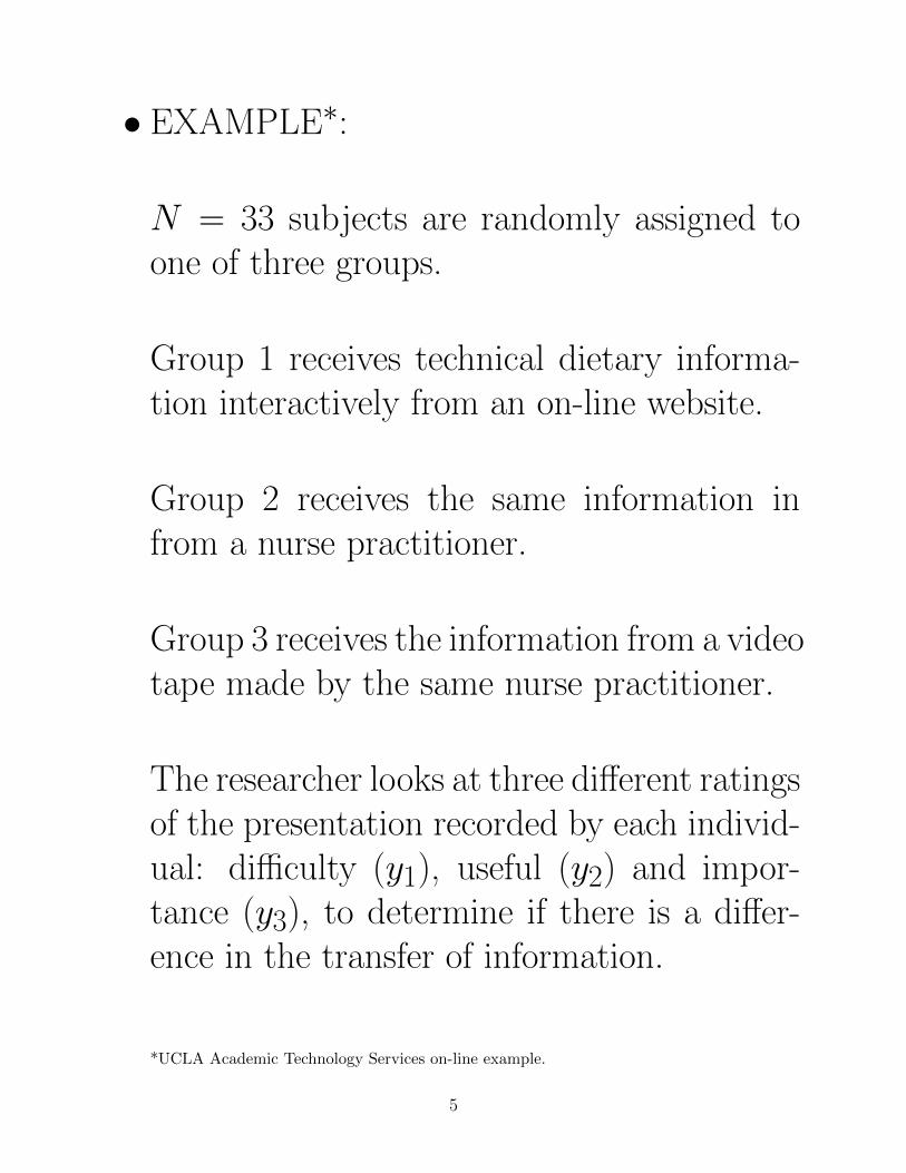
• EXAMPLE∗:
N = 33 subjects are randomly assigned toone of three groups.
Group 1 receives technical dietary informa-tion interactively from an on-line website.
Group 2 receives the same information infrom a nurse practitioner.
Group 3 receives the information from a videotape made by the same nurse practitioner.
The researcher looks at three different ratingsof the presentation recorded by each individ-ual: difficulty (y1), useful (y2) and impor-tance (y3), to determine if there is a differ-ence in the transfer of information.
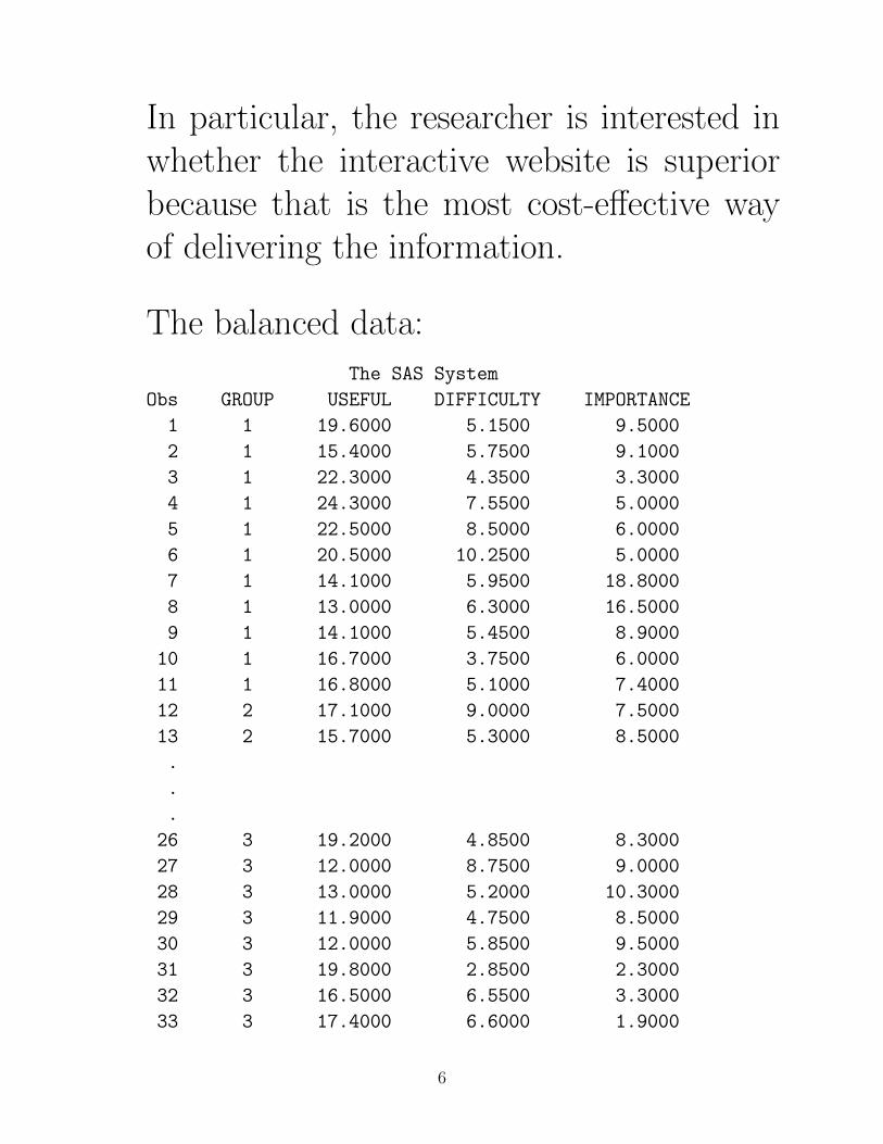
In particular, the researcher is interested inwhether the interactive website is superiorbecause that is the most cost-effective wayof delivering the information.
The balanced data:
The SAS System
Obs GROUP USEFUL DIFFICULTY IMPORTANCE
1 1 19.6000 5.1500 9.5000
2 1 15.4000 5.7500 9.1000
3 1 22.3000 4.3500 3.3000
4 1 24.3000 7.5500 5.0000
5 1 22.5000 8.5000 6.0000
6 1 20.5000 10.2500 5.0000
7 1 14.1000 5.9500 18.8000
8 1 13.0000 6.3000 16.5000
9 1 14.1000 5.4500 8.9000
10 1 16.7000 3.7500 6.0000
11 1 16.8000 5.1000 7.4000
12 2 17.1000 9.0000 7.5000
13 2 15.7000 5.3000 8.5000
.
.
.
26 3 19.2000 4.8500 8.3000
27 3 12.0000 8.7500 9.0000
28 3 13.0000 5.2000 10.3000
29 3 11.9000 4.7500 8.5000
30 3 12.0000 5.8500 9.5000
31 3 19.8000 2.8500 2.3000
32 3 16.5000 6.5500 3.3000
33 3 17.4000 6.6000 1.9000
6
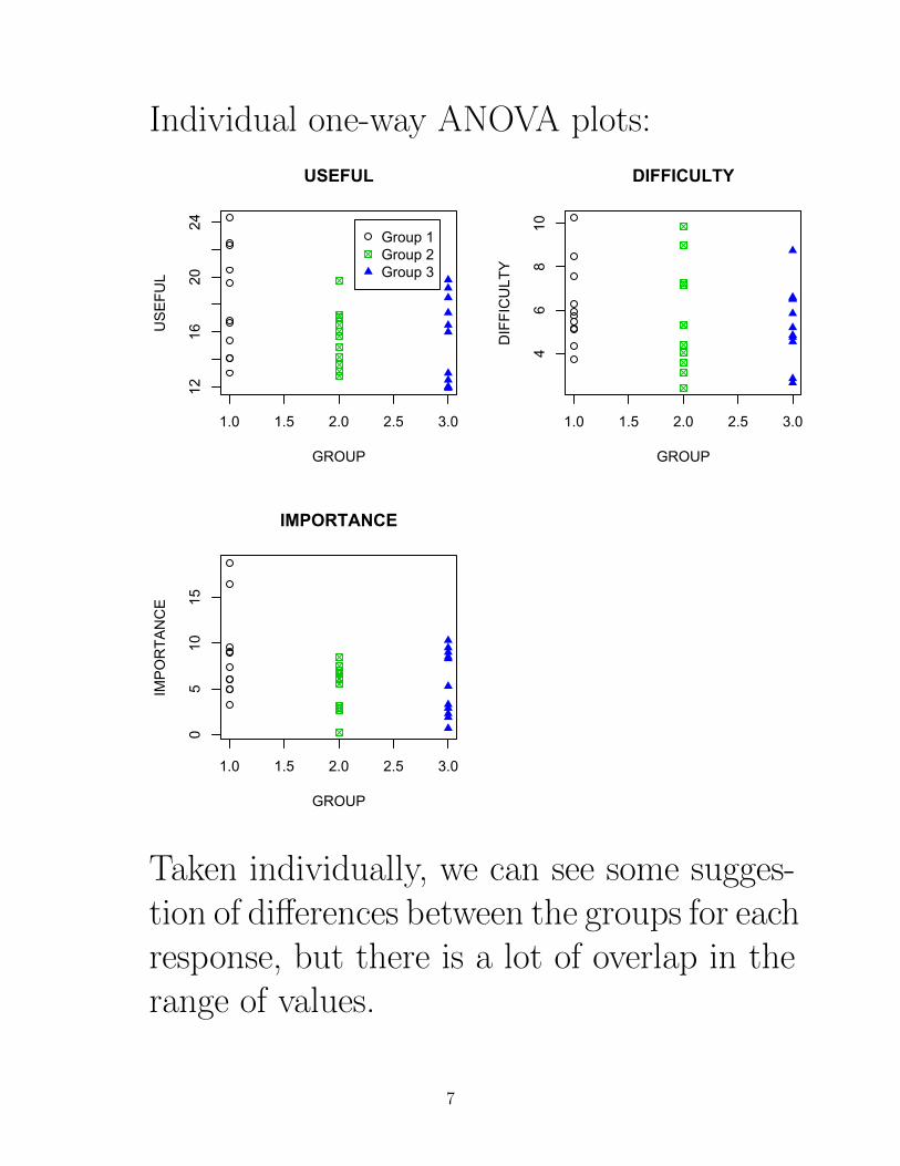
Individual one-way ANOVA plots:
1.0 1.5 2.0 2.5 3.0
1216
2024
USEFUL
GROUP
USEFUL
Group 1Group 2Group 3
1.0 1.5 2.0 2.5 3.0
46
810
DIFFICULTY
GROUP
DIFFICULTY
1.0 1.5 2.0 2.5 3.0
05
1015
IMPORTANCE
GROUP
IMPORTANCE
Taken individually, we can see some sugges-tion of differences between the groups for eachresponse, but there is a lot of overlap in therange of values.
7
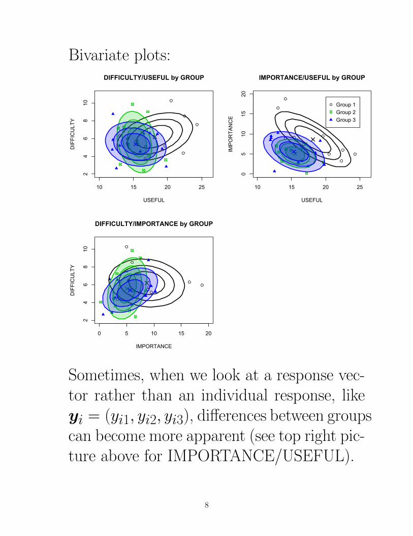
Bivariate plots:
10 15 20 25
24
68
10DIFFICULTY/USEFUL by GROUP
USEFUL
DIFFICULTY
10 15 20 25
05
1015
20
IMPORTANCE/USEFUL by GROUP
USEFUL
IMPORTANCE
Group 1Group 2Group 3
0 5 10 15 20
24
68
10
DIFFICULTY/IMPORTANCE by GROUP
IMPORTANCE
DIFFICULTY
Sometimes, when we look at a response vec-tor rather than an individual response, likeyi = (yi1, yi2, yi3), differences between groupscan become more apparent (see top right pic-ture above for IMPORTANCE/USEFUL).
8
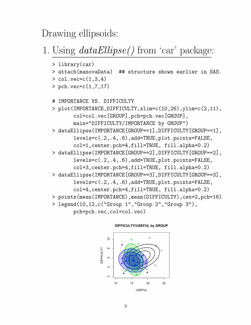
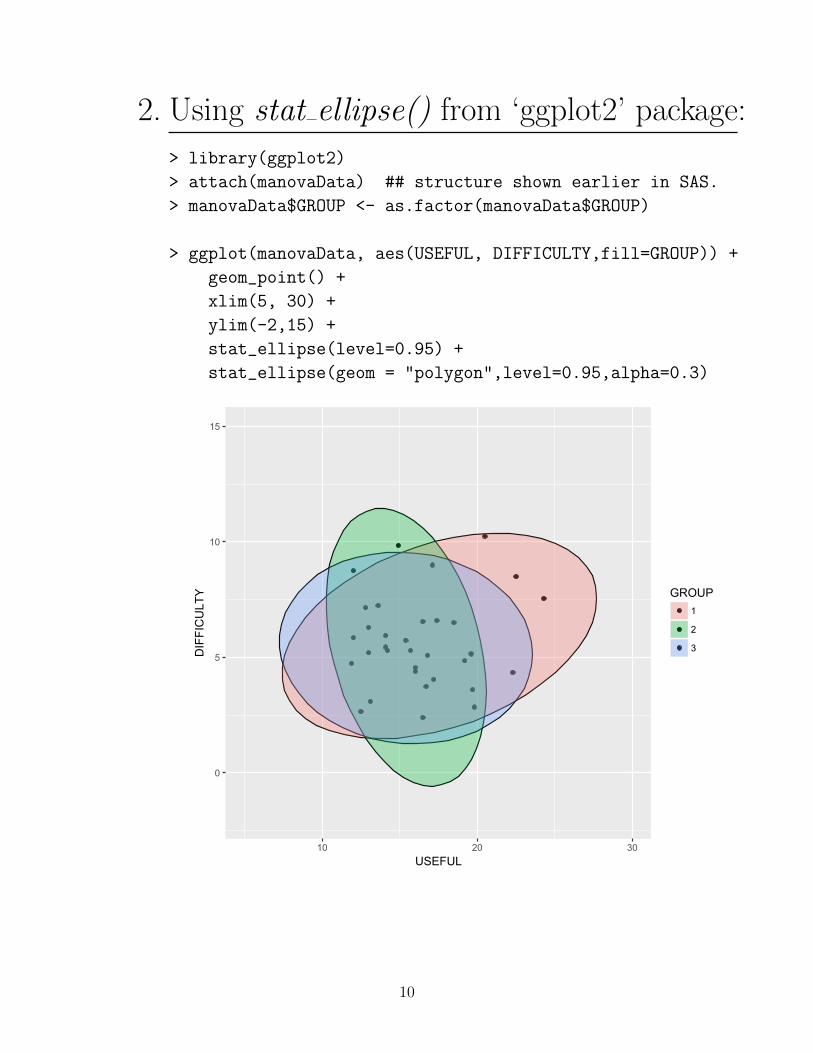
Drawing ellipsoids:
1. Using dataEllipse() from ‘car’ package:> library(car)
> attach(manovaData) ## structure shown earlier in SAS.
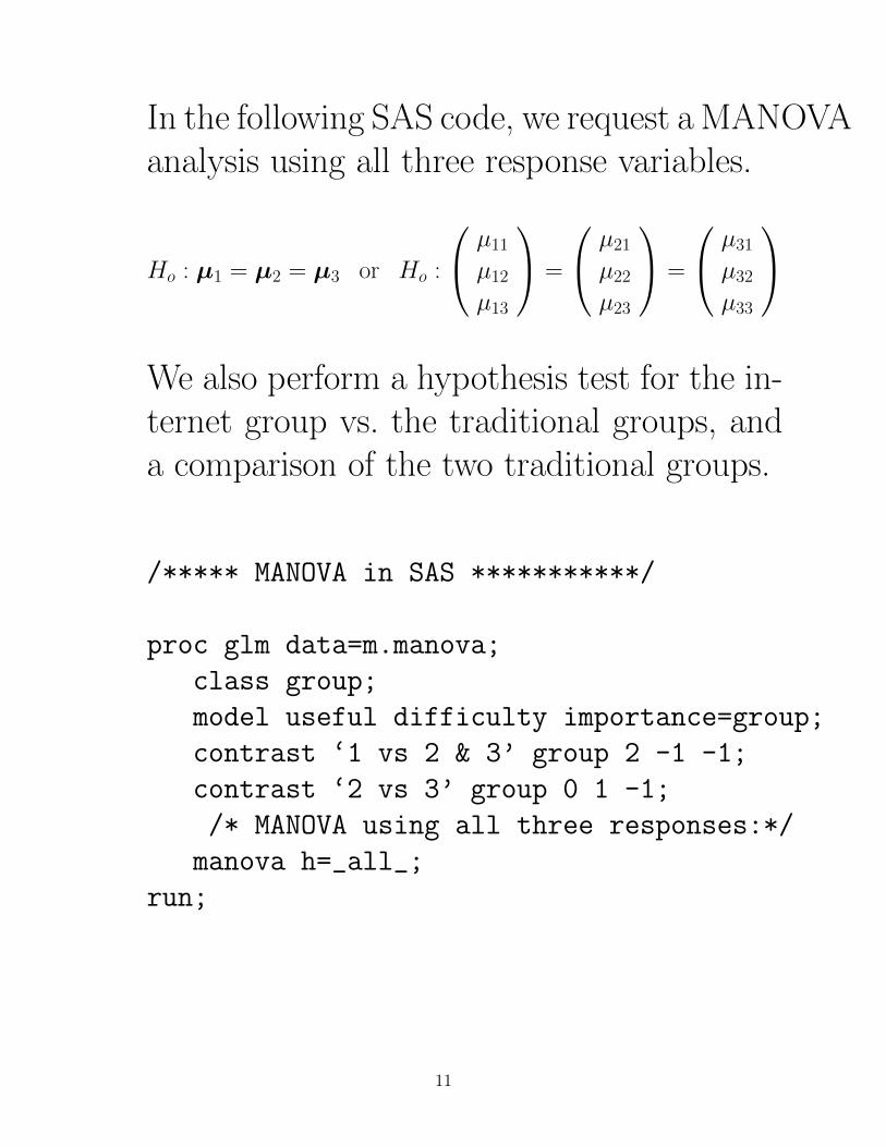
In the following SAS code, we request a MANOVAanalysis using all three response variables.
Ho : µ1 = µ2 = µ3 or Ho :
µ11µ12µ13
=
µ21µ22µ23
=
µ31µ32µ33
We also perform a hypothesis test for the in-ternet group vs. the traditional groups, anda comparison of the two traditional groups.
/***** MANOVA in SAS ***********/
proc glm data=m.manova;
class group;
model useful difficulty importance=group;
contrast ‘1 vs 2 & 3’ group 2 -1 -1;
contrast ‘2 vs 3’ group 0 1 -1;
/* MANOVA using all three responses:*/
manova h=_all_;
run;
11
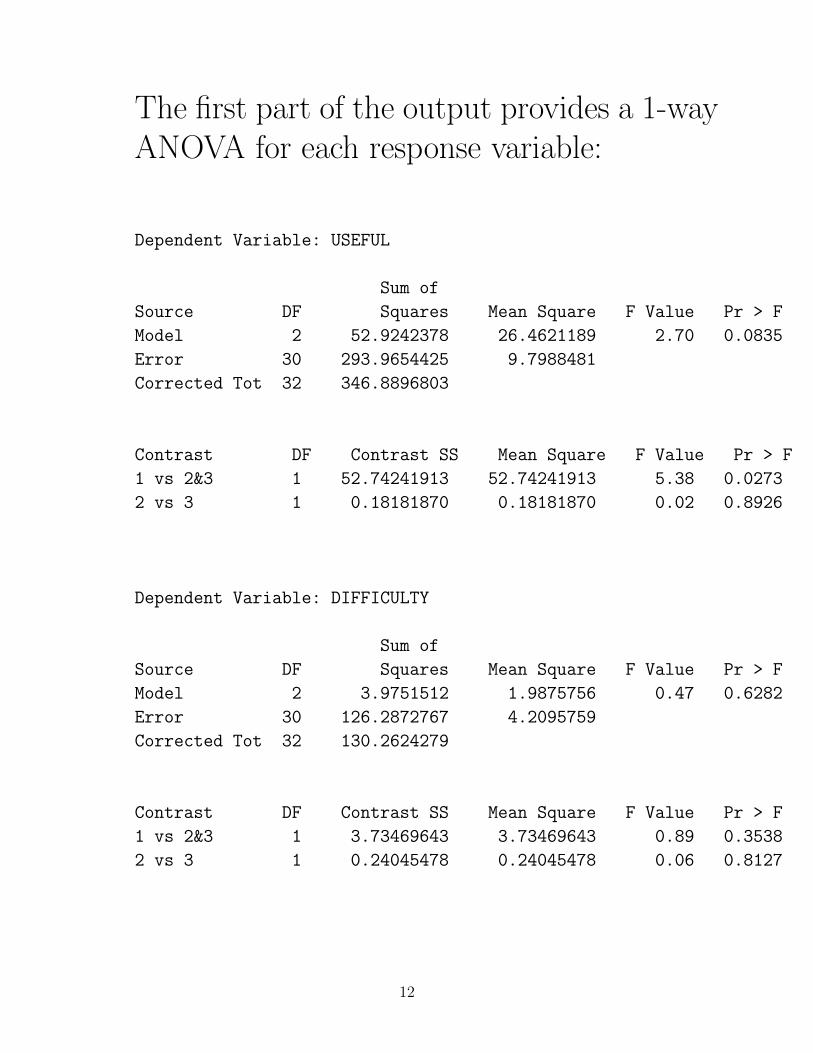
The first part of the output provides a 1-wayANOVA for each response variable:
Dependent Variable: USEFUL
Sum of
Source DF Squares Mean Square F Value Pr > F
Model 2 52.9242378 26.4621189 2.70 0.0835
Error 30 293.9654425 9.7988481
Corrected Tot 32 346.8896803
Contrast DF Contrast SS Mean Square F Value Pr > F
1 vs 2&3 1 52.74241913 52.74241913 5.38 0.0273
2 vs 3 1 0.18181870 0.18181870 0.02 0.8926
Dependent Variable: DIFFICULTY
Sum of
Source DF Squares Mean Square F Value Pr > F
Model 2 3.9751512 1.9875756 0.47 0.6282
Error 30 126.2872767 4.2095759
Corrected Tot 32 130.2624279
Contrast DF Contrast SS Mean Square F Value Pr > F
1 vs 2&3 1 3.73469643 3.73469643 0.89 0.3538
2 vs 3 1 0.24045478 0.24045478 0.06 0.8127
12
The GLM Procedure
Dependent Variable: IMPORTANCE
Sum of
Source DF Squares Mean Square F Value Pr > F
Model 2 81.8296936 40.9148468 2.88 0.0718
Error 30 426.3708962 14.2123632
Corrected Tot 32 508.2005898
Contrast DF Contrast SS Mean Square F Value Pr > F
1 vs 2&3 1 80.30060224 80.30060224 5.65 0.0240
2 vs 3 1 1.52909132 1.52909132 0.11 0.7452
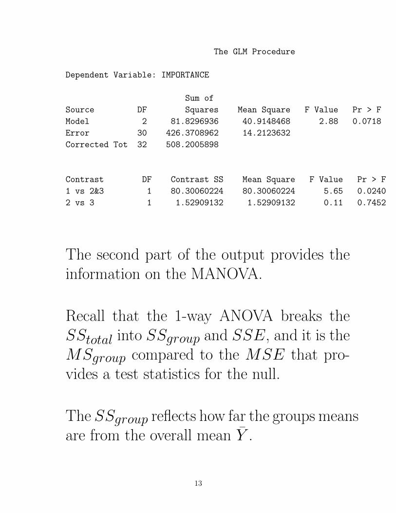
The second part of the output provides theinformation on the MANOVA.
Recall that the 1-way ANOVA breaks theSStotal into SSgroup and SSE, and it is theMSgroup compared to the MSE that pro-vides a test statistics for the null.
The SSgroup reflects how far the groups meansare from the overall mean Y .
13
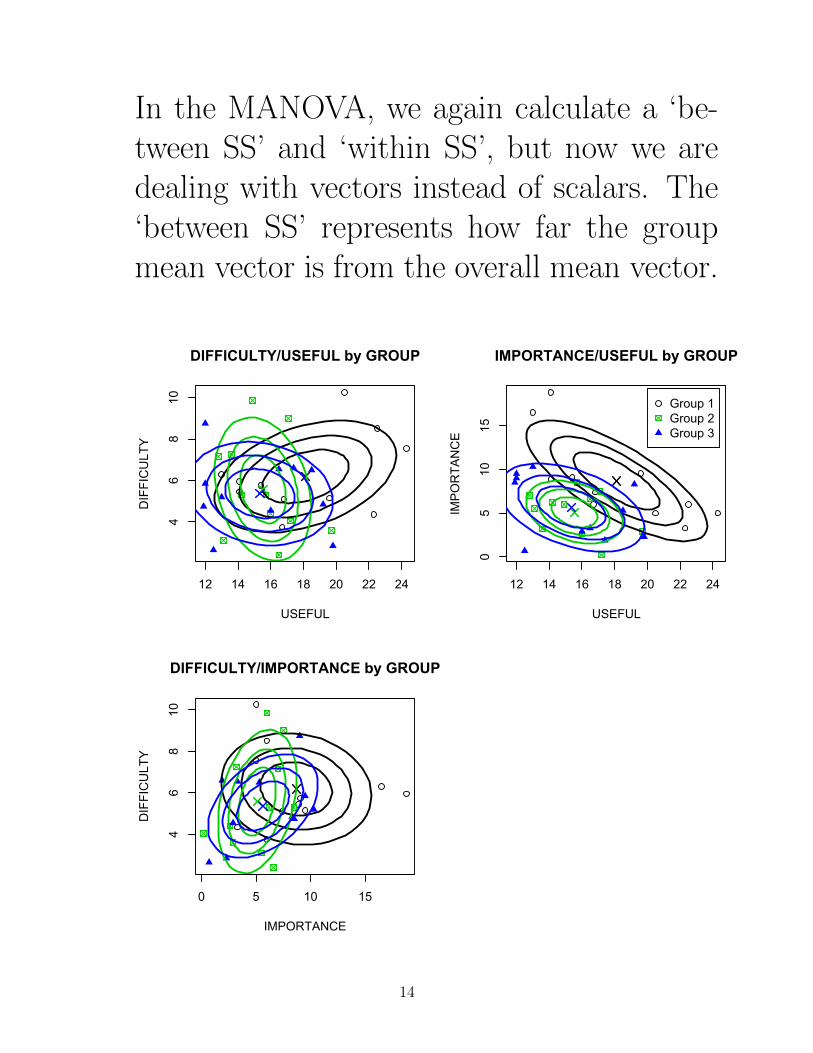
In the MANOVA, we again calculate a ‘be-tween SS’ and ‘within SS’, but now we aredealing with vectors instead of scalars. The‘between SS’ represents how far the groupmean vector is from the overall mean vector.
12 14 16 18 20 22 24
46
810
DIFFICULTY/USEFUL by GROUP
USEFUL
DIFFICULTY
12 14 16 18 20 22 24
05
1015
IMPORTANCE/USEFUL by GROUP
USEFUL
IMPORTANCE
Group 1Group 2Group 3
0 5 10 15
46
810
DIFFICULTY/IMPORTANCE by GROUP
IMPORTANCE
DIFFICULTY
14
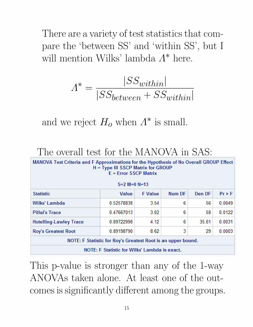
There are a variety of test statistics that com-pare the ‘between SS’ and ‘within SS’, but Iwill mention Wilks’ lambda Λ∗ here.
Λ∗ =|SSwithin|
|SSbetween + SSwithin|
and we reject Ho when Λ∗ is small.
The overall test for the MANOVA in SAS:
This p-value is stronger than any of the 1-wayANOVAs taken alone. At least one of the out-comes is significantly different among the groups.
15
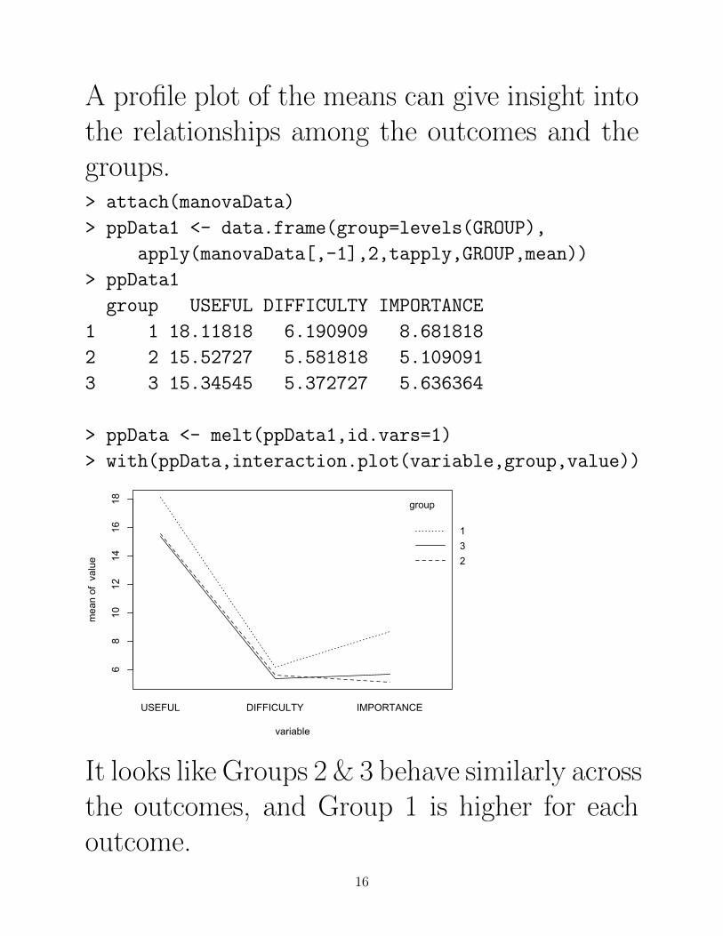
A profile plot of the means can give insight intothe relationships among the outcomes and thegroups.> attach(manovaData)
It looks like Groups 2 & 3 behave similarly acrossthe outcomes, and Group 1 is higher for eachoutcome.
16
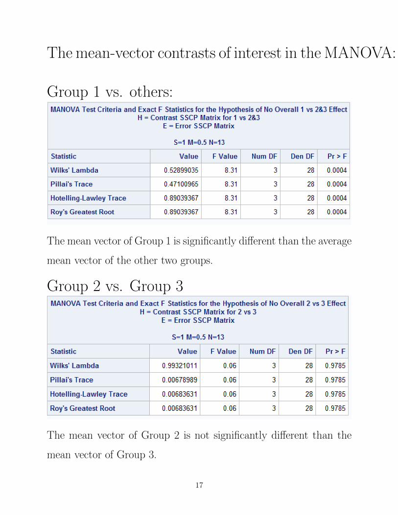
The mean-vector contrasts of interest in the MANOVA:
Group 1 vs. others:
The mean vector of Group 1 is significantly different than the average
mean vector of the other two groups.
Group 2 vs. Group 3
The mean vector of Group 2 is not significantly different than the
mean vector of Group 3.
17
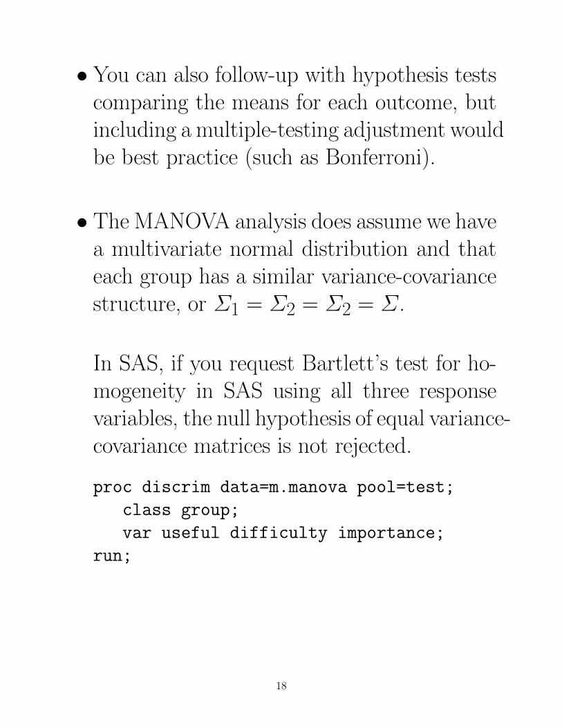
• You can also follow-up with hypothesis testscomparing the means for each outcome, butincluding a multiple-testing adjustment wouldbe best practice (such as Bonferroni).
• The MANOVA analysis does assume we havea multivariate normal distribution and thateach group has a similar variance-covariancestructure, or Σ1 = Σ2 = Σ2 = Σ.
In SAS, if you request Bartlett’s test for ho-mogeneity in SAS using all three responsevariables, the null hypothesis of equal variance-covariance matrices is not rejected.
proc discrim data=m.manova pool=test;
class group;
var useful difficulty importance;
run;
18
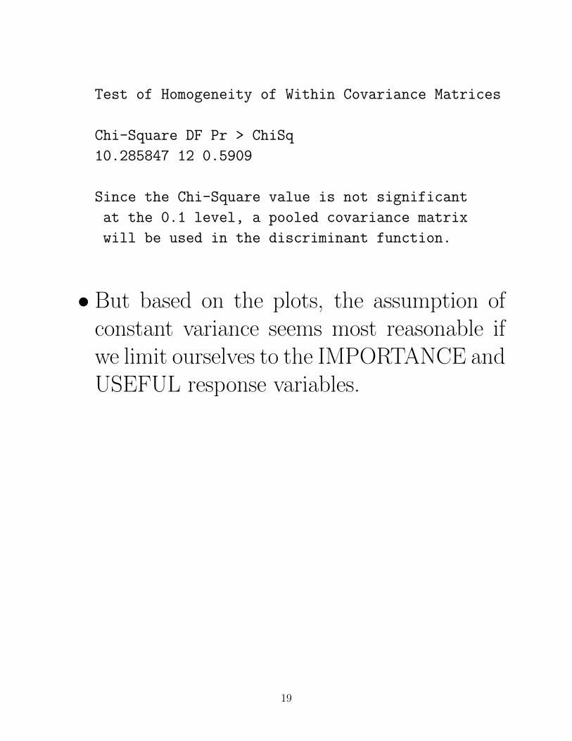
Test of Homogeneity of Within Covariance Matrices
Chi-Square DF Pr > ChiSq
10.285847 12 0.5909
Since the Chi-Square value is not significant
at the 0.1 level, a pooled covariance matrix
will be used in the discriminant function.
• But based on the plots, the assumption ofconstant variance seems most reasonable ifwe limit ourselves to the IMPORTANCE andUSEFUL response variables.
19
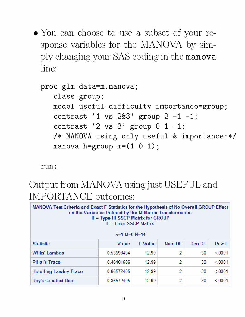
• You can choose to use a subset of your re-sponse variables for the MANOVA by sim-ply changing your SAS coding in the manovaline:
proc glm data=m.manova;
class group;
model useful difficulty importance=group;
contrast ‘1 vs 2&3’ group 2 -1 -1;
contrast ‘2 vs 3’ group 0 1 -1;
/* MANOVA using only useful & importance:*/
manova h=group m=(1 0 1);
run;
Output from MANOVA using just USEFUL andIMPORTANCE outcomes:
20
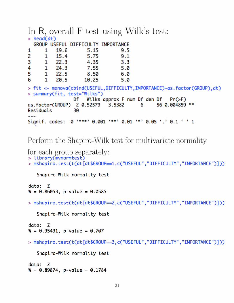
In R, overall F-test using Wilk’s test:
Perform the Shapiro-Wilk test for multivariate normality
for each group separately:
21
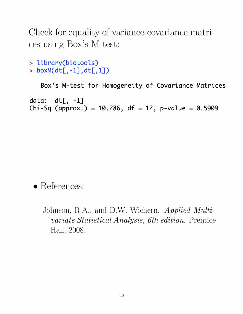
Check for equality of variance-covariance matri-ces using Box’s M-test: