STATISTICAL CONTROVERSIES IN CENSUS 2000 30 April 1999

Technical Report 537, Department of Statistics, U.C. BerkeleyTo appear inJurimetrics

by Lawrence D. Brown, Morris L. Eaton, David A. Freedman, Stephen P. Klein, Richard A. Olshen,Kenneth W. Wachter, Martin T. Wells, and Donald Ylvisaker.

ABSTRACT

This paper is a discussion of Census 2000, focusing on planned use of samplingtechniques for adjustment. Past experience with similar adjustment methodssuggests that the design for Census 2000 is quite risky. Adjustment was thefocus of litigation in the census of 1980 and 1990. The planned use of samplingto obtain population counts for apportionment was rejected by the SupremeCourt as violating the Census Act. Statistical adjustments for the purpose ofredistricting may or may not be constitutional.

I. INTRODUCTION

The census has been the subject of high-profile controversy since the 1980s.1 In 1980 and1990, the major cases revolved around proposed adjustments to remedy the differential undercountof minorities. For Census 2000, sampling was the focus of the conflict. Sampling came into theBureau’s proposed design in two main ways.

(i) Only a sample of households that do not respond to the census by mail was to be followedup by interviewers; in the past, all non-responding households were followed up.

(ii) A large sample survey after the enumeration was to be used as the basis for adjustmentof census counts to compensate for under- and over-enumeration. This use of samplingwas called “ICM” or “Integrated Coverage Measurement.”

Sample-based non-response followup has been dropped from the plan, since the courts have ruledthat this use of sampling—for purposes of apportionment—would violate the Census Act.2 That isthe topic of Section II.

Despite the name, ICM is not an inseparable part of the census operation. Instead, it is a largerversion of the Post Enumeration Survey (PES) that was developed for adjusting the census in 1990.In turn, the PES was a modification of the “Post Enumeration Program” for the census of 1980.These proposals for adjustment are all based on a capture-recapture technique called “dual systemestimation:” capture is in the census, recapture is in the post enumeration survey. Details are givenbelow. The ICM is still part of the Bureau’s plan for Census 2000, although the acronym has beenchanged to ACE (Accuracy and Coverage Evaluation). The focus of Sections III–X is the plan forCensus 2000 that was reviewed by the courts, although most of the statistical considerations applyas well to the current plan for ACE (Section XI).

In the past, there have been census undercounts that differ by race and ethnicity, sex, andage. Such differentials can distort political representation and the allocation of tax funds. Adjust-ment is meant to correct these inequities by changing the way resources are shared out. However,

1

adjustment creates no new resources. Furthermore, political representation and tax funds are gen-erally allocated to geographical areas rather than national racial or ethnic groups. For such reasons,the population shares of places—such as states, counties, and cities—matter more than counts.Improving the accuracy of population shares for places is more delicate than improving nationalcounts of demographic groups. Unless the adjustment method is quite exact, it can make estimatedshares worse by putting people in the wrong places. For 1990, there were major errors in theproposed adjustments, as shown by Census Bureau evaluation data: adjustment could easily havemade population shares less accurate rather than more accurate, even for states.

The 1990 census counted 248.7 million people. As of July 1991, the undercount in thecensus was estimated as 2.1%, or 5.3 million people (net, nationwide). The median change in statepopulation shares that would have been produced by adjustment was 8 parts in 100,000; signs areignored in this calculation. Share changes are what need to be estimated, and estimating at thelevel of 1 in 10,000 or 1 in 100,000 is obviously a difficult business. The difficulty is compoundedbecause the census includes both overcounts and undercounts: the net undercount is the differencebetween two much larger numbers. That kind of subtraction entails a substantial loss in accuracy(Section III).

Sample-based estimates suffer from sampling error and non-sampling error. The latter was byfar the more serious problem in 1990 and is likely to be so again in 2000, as discussed below. Thesalient points are as follows.

(i) Processing errors in the PES.The census makes errors of various kinds; so does the postenumeration survey. Some of the estimated undercount must result from census errors,but some is due to processing errors in the PES. In 1990, of the 5.3 million estimatedundercount, processing errors in the PES contributed roughly 3 to 4 million. (Thesefigures are net, and national in scope; Section IVA.)

(ii) Correlation bias.Some kinds of people are missed both in the original census and in theadjusted census. Such people are unlikely to be randomly distributed over the landscape,and there are enough of them to matter (Section V).

(iii) Heterogeneity.Geographical shares are adjusted by assuming that undercount rates areconstant within specific demographic groups called “post strata.” This assumption isclearly wrong (Section VI).

(iv) Instability. Adjustment depends on a host of somewhat arbitrary technical decisions, someof which have a considerable bearing on the results. For example, in 1990, estimates of theundercount were smoothed using a hierarchical Bayes sort of procedure. However, therewas a decision to “pre-smooth” the variances going into the algorithm, using yet anotherprocedure. Pre-smoothing more or less doubled the estimated undercount (Section VIIB).

Efforts to demonstrate the validity of adjustment are more problematic than adjustment itself, be-cause they depend even more heavily on assumptions that turn out to be rather fragile (Section VIII).Sampling for non-response will be discussed in Section IX, and some of the arguments in favor ofsampling are reviewed in Section X.

In 1980 and 1990, suits were brought by the City of New York among other plaintiffs tocompel adjustment, but the courts held that the federal government’s decision not to adjust wasreasonable, and strict scrutiny was not required.3 With Census 2000, there were challenges tosampling as a method of determining the population base for apportionment, that is, the distribution

2

of congressional seats among the states. The arguments were more legal than statistical, andprevailed in court—as discussed in the next section.

II. LEGAL BACKGROUND

To resolve a conflict over funding, Congress enacted statutes requiring the Bureau to reportits plans for taking the 2000 census, deeming these plans to be final agency action, and authorizingthe Speaker of the House to sue the Department of Commerce to preclude use of sampling forapportionment; such cases were to be heard by a three-judge panel, with expedited review by theSupreme Court.4 The Executive Branch argued that the Congress had no standing to bring the suit;among other things, only a future Congress would have its electoral districts affected by sampling.Furthermore, the matter was not ripe for adjudication because Congress could for instance denyfunds for sampling. The district court rejected these arguments in U.S. House of Representativesv. U.S. Department of Commerce, et al.5

Without holding that 105th House is itself either the “next friend” of or a fiduciary for the107th House, we hold that because of the special relationship between the present Houseand its successor once removed, the 105th House has standing to litigate on behalf of the107th House. This permits the current House to vindicate the later House’s interest in ful-filling its constitutional duties regarding the census, without giving rise to general legislativestanding. . . .6

If this court does not rule on this question now, and thereafter a reviewing court concludespost-census that statistical sampling is statutorily or constitutionally proscribed, it will beimpossible at that point to determine what the headcount-only number would have been.7

We turn now to the core issue. The Census Act governs the taking of the census. According to the1957 version of section 195,

except for the determination of the population for apportionment purposes, the Secretary [ofCommerce] may, where he deems it appropriate, authorize the use of the statistical methodknown as “sampling” in carrying out the provisions of this title.8

The Census Act was amended in 1976, and the revised version of Section 195 recommendedsampling more strongly:

except for the determination of the population for purposes of apportionment of Representativesin Congress among the several States, the Secretary shall, if he considers it feasible, authorizethe use of the statistical method known as “sampling” in carrying out the provisions of thistitle.

The Executive Branch, however, relied on Section 141(a) of the 1976 Act:

The Secretary shall, in the year 1980 and every 10 years thereafter, take a decennial census ofpopulation as of the first day of April of such year, which date shall be known as the “decennialcensus date” in such form and content as he may determine, including the use of samplingprocedures and special surveys.9

The court held that the grant of authority in Section 141 was qualified by the restriction in Section195, the latter being more specific and therefore binding.10 In sum,

3

Reading section 141(a) and section 195 together, and considering the plain text, legislativehistory, and other tools of statutory construction, this court finds that the use of statisticalsampling to determine the population for purposes of the apportionment of representatives inCongress among the states violates the Census Act.11

The constitution requires an “actual enumeration of the population:” the Speaker argued thatthe constitutional language precluded adjustment, but the court ruled that “there is no need toreach the constitutional questions presented.”12 In a summary judgment, the court enjoined theDepartment of Commerce “from using any form of statistical sampling, including their programfor nonresponse follow-up and Integrated Coverage Measurement, to determine the population forpurposes of congressional apportionment.”13

A parallel case, Matthew Glavin, et al. v. William J. Clinton, et al.14 was initiated by theSoutheastern Legal Foundation, with similar results. Plaintiffs included several individuals livingin different states; there was also a corporate plaintiff, Cobb County (Georgia). The argument onstanding was somewhat different: according to the Executive Branch, plaintiffs lacked standingsince there was no proof of harm. However, the court held that harm was probable, since resultsof adjustment in 2000 were likely to be similar to results in 1990. Vote dilution and loss of federalfunds were concrete injuries likely to flow from adjustment, and “plaintiffs do not need to prove withmathematical certainty the degree to which they will be injured. . . .”15 The court found that “theonly plausible interpretation of the plain language and structure of the [Census] Act is that Section195 prohibits sampling for apportionment and Section 141 allows it for all other purposes.”16 Thecourt granted plaintiffs motion for summary judgment, ordering “that the defendants should bepermanently enjoined from using any form of statistical sampling, including their program fornonresponse follow-up and Integrated Coverage Measurement, to determine the population forpurposes of congressional apportionment.”17

A divided Supreme Court upheld the decisions of the lower courts.18 The opinion focused onGlavin, summarized as follows.

The District Court held that the case was ripe for review, that the plaintiffs satisfied therequirements for Article III standing, and that the Census Act prohibited use of the challengedsampling procedures to apportion Representatives. 19 F.Supp. 2d, at 547, 548–550, 553. TheDistrict Court concluded that, because the statute was clear on its face, the court did not need toreach the constitutional questions presented. Id., at 553. It thus denied defendants’ motion todismiss, granted plaintiffs’ motion for summary judgment, and permanently enjoined the use ofthe challenged sampling procedures to determine the population for purposes of congressionalapportionment. Id., at 545, 553.19

With respect to the issues of standing and ripeness, the Supreme Court reasoned as follows.

. . . . because the record before us amply supports the conclusion that several of the ap-pellees have met their burden of proof regarding their standing to bring this suit, we affirm theDistrict Court’s holding.20

[One plaintiff was a resident of Indiana, whose] expected loss of a Representative tothe United States Congress undoubtedly satisfies the injury-in-fact requirement of Article IIIstanding. In the context of apportionment, we have held that voters have standing to challengean apportionment statute because “[t]hey are asserting ‘a plain, direct and adequate interestin maintaining the effectiveness of their votes.’” Baker v. Carr, 369 U.S. 186, 208 (1962)

4

(quoting Coleman v. Miller, 307 U.S. 433, 438 (1939)). The same distinct interest is at issuehere: With one fewer Representative, Indiana residents’ votes will be diluted. Moreover, thethreat of vote dilution through the use of sampling is “concrete” and “actual or imminent, not‘conjectural’ or ‘hypothetical.’” Whitmore v. Arkansas, 495 U.S. 149, 155 (1990).21

And it is certainly not necessary for this Court to wait until the census has been conductedto consider the issues presented here, because such a pause would result in extreme—possiblyirremediable—hardship. . . . There is undoubtedly a “traceable” connection between the useof sampling in the decennial census and Indiana’s expected loss of a Representative, andthere is a substantial likelihood that the requested relief—a permanent injunction against theproposed uses of sampling in the census—will redress the alleged injury. . . . Appellees havealso established standing on the basis of the expected effects of the use of sampling in the 2000census on intrastate redistricting.22

Thus, the appellees who live in the aforementioned counties have a strong claim that theywill be injured by the Bureau’s plan because their votes will be diluted vis-a-vis residents ofcounties with larger “undercount” rates. . . . For the reasons discussed above. . . , this expectedintrastate vote dilution satisfies the injury-in-fact, causation, and redressibility requirements.Accordingly, appellees have again carried their burden under Rule 56 and have establishedstanding to pursue this case.23

A majority of the Court continued,

We accordingly arrive at the dispute over the meaning of the relevant provisions of theCensus Act. The District Court below examined the plain text and legislative history of theAct and concluded that the proposed use of statistical sampling to determine population forpurposes of apportioning congressional seats among the States violates the Act. We agree.24

This broad grant of authority given in §141(a) is informed. . . by the narrower and morespecific §195, which is revealingly entitled, “Use of Sampling.” See Green v. Bock LaundryMachine Co., 490 U.S. 504, 524 (1989). The §141 authorization to use sampling techniquesin the decennial census is not necessarily an authorization to use these techniques in collectingall of the information that is gathered during the decennial census. We look to the remainderof the law to determine what portions of the decennial census the authorization covers. Whenwe do, we discover that. . . §195 directly prohibits the use of sampling in the determinationof population for purposes of apportionment. [footnote omitted.]25

As amended, the section now requires the Secretary to use statistical sampling in assem-bling the myriad demographic data that are collected in connection with the decennial census.But the section maintains its prohibition on the use of statistical sampling in calculating pop-ulation for purposes of apportionment. Absent any historical context, the language in theamended §195 might reasonably be read as either permissive or prohibitive with regard to theuse of sampling for apportionment purposes.26

Here, the context is provided by over 200 years during which federal statutes have pro-hibited the use of statistical sampling where apportionment is concerned. In light of thisbackground, there is only one plausible reading of the amended §195: It prohibits the use ofsampling in calculating the population for purposes of apportionment.27

5

The majority concluded,

For the reasons stated, we conclude that the Census Act prohibits the proposed uses ofstatistical sampling in calculating the population for purposes of apportionment. Becausewe so conclude, we find it unnecessary to reach the constitutional question presented. . . .

Accordingly, we affirm the judgment of the District Court for the Eastern District of Virginia inClinton v. Glavin, No. 98–564. As this decision also resolves the substantive issues presentedby Department of Commerce v. United States House of Representatives, No. 98–404, thatcase no longer presents a substantial federal question. The appeal in that case is thereforedismissed.28

In response to this decision, the Executive Branch now seems to be planning a two-trackcensus, with a headcount for apportionment, while adjusted counts are used for redistricting withinstate and allocation of federal funds (Section XI below). Sample-based non-response followuphad to be dropped: if 100% followup is needed for apportionment, it would not be sensible to dosample-based followup in parallel for other purposes.

The Executive Branch is required by law to release the unadjusted block counts:

In both the 2000 decennial census, and any dress rehearsal or other simulation made in prepara-tion for the 2000 decennial census, the number of persons enumerated without using statisticalmethods must be publicly available for all levels of census geography which are being re-leased by the Bureau of the Census for: (1) all data releases before January 1, 2001, (2) thedata contained in the 2000 decennial census Public Law 94-171 data file released for use inredistricting, (3) the Summary Tabulation File One (STF-1) for the 2000 decennial census; and(4) the official populations of the States transmitted from the Secretary of Commerce throughthe President to the Clerk of the House used to reapportion the districts of the House amongthe States as a result of the 2000 decennial census.29

Some states may elect to use the unadjusted counts for redistricting, while others will use theadjusted figures. Litigation seems inevitable. Many plaintiffs are likely to have standing, but theconstitutionality of sample-based adjustments remains to be decided. The balance of the presentarticle mainly considers the statistical issues raised by adjustment. These issues were not prominentin the litigation about use of sampling for apportionment, but may become quite salient in litigationprompted by redistricting.

III. INTEGRATED COVERAGE MEASUREMENT

The version of ICM reviewed by the courts was to be based on a PES or post enumerationsurvey—a cluster sample of about 60,000 blocks, containing 750,000 housing units and 1.7 millionpeople. A “block” is the minimal unit of census geography: there are about 7 million blocks inthe U.S., of which about 5 million are inhabited. The discussion that follows applies to the PESof 1990 as well as 2000; some differences of detail will be noted below. A listing is made ofthe housing units in the sample blocks, and persons in these units are interviewed after the censusis complete. PES records are then matched against census records. A match generally validatesboth the census record and the PES record. A PES record that does not match to the census maycorrespond to a gross omission, that is, a person who should have been counted in the census but wasmissed. Conversely, a census record that does not match to the PES may correspond to an erroneous

6

enumeration, that is, a person who was counted in the census in error. For example, someone maybe counted twice in the census—perhaps because he sent in two forms, and quality control failed toidentify the duplication. Another person may be counted correctly but assigned to the wrong unit ofgeography. She would be a gross omission in one place and an erroneous enumeration in the other.Census records fabricated by respondents or enumerators would also be erroneous enumerations.The main purpose of the post enumeration survey is to estimate the number of gross omissions anderroneous enumerations.

July 15, 1991 was a critical date for the 1990 PES because the Secretary of Commerce hadthen to decide whether or not to adjust the 1990 census. He decided not to adjust, over-ruling inthe process a split recommendation from the technical staff at the Bureau of the Census. At thetime, results from the post enumeration survey of 1990 suggested there were about 19 million grossomissions and 13 million erroneous enumerations; 2 million persons in the census had insufficientdata for matching.30 A first approximation to the estimated undercount is 19− 13− 2 = 4 million;another million persons were added by statistical modeling. Relatively small errors in estimatingthe number of gross omissions and erroneous enumerations can lead to an unacceptably large errorin the difference of the two—and it is the difference that is relevant. For example, if the grossomissions are overestimated by 10% and the erroneous enumerations are underestimated by 10%,the undercount is overestimated by 1.9+ 1.3 = 3.2 million. In combination, the two errors of 10%create an error that exceeds 60% of the estimated undercount. The next section provides furtherdetail, and shows that our illustrative calculation is realistic.

“Non-sampling error” is a catch-all term for errors other than sampling error. Respondentsgive answers that are not wholly correct. There are clerical errors in processing data. There aresystematic biases in matching and in models used to impute missing data. There are differentialsuccess rates in finding persons omitted from the census. Sampling error can be expected to godown with bigger samples, but non-sampling error is another story. As sample size increases, itbecomes more difficult to recruit, train, and manage personnel. Moreover, complexity increasesthe likelihood of non-sampling error. Adjustment programs like the PES are most vulnerable tonon-sampling error, and it is non-sampling error that is hard to control—or even to quantify.

Generally, the post enumeration survey proposed for 2000 is close in design to the one for 1990.However, matching will be done on site during the interview, not afterwards at field offices; moverswill be handled differently; and the sample is larger.31 Erroneous enumerations are likely to beeven more numerous in 2000 than in 1990 because in 2000 the Census Bureau will be broadcastingthe forms in many different ways in its “Be Counted” program.32 The Bureau will use computeralgorithms to detect and remove duplicates; the reliability of these algorithms is presently unknown.Differences between Census 2000 and 1990 will be discussed in more detail below.

IV. PROCESSING ERROR

IV A. Evaluation Data

Some systematic error is inevitable in any large survey operation. The PES is particularlyvulnerable to such error for two reasons mentioned above: (i) the adjustments to state shares thatneed to be estimated are tiny, and (ii) relatively small errors in estimates of gross omissions anderroneous enumerations translate into relatively large errors for the net undercount. Moreover, thePES will be conducted under extreme time pressure to meet the legal deadline for the transmission

7

of census data to Congress. Processing errors are likely to be even more serious in 2000 than theywere in 1990: the larger sample size and the tighter timetable make quality control more difficult.

The plan to conduct initial matching on site could make it easier to resolve cases by questioningthe respondents. On the other hand, enumerators may prove less adept than the specialized matchersof 1990. The fieldwork will be done closer to census day, which should reduce the number ofbad census day addresses given by respondents; avoiding interactions between census and PESoperations will be harder.

Matching people between two large sets of records (the census and the PES) is a complex anderror-prone process. Due to concerns about confidentiality, the census cannot collect unique iden-tifiers, like fingerprints or social security numbers. Instead, records are matched using incompleteand sometimes erroneous data provided by the respondents. One of the paradoxes of adjustmentis that matching is hardest to do in the geographical areas that are hardest to count.33 Therefore,errors introduced by adjustment are far from evenly distributed.

In 1990, the Census Bureau conducted extensive evaluations of the adjustment-related oper-ations, including reinterviewing samples of households and rematching samples of records. (Thereinterviewing was done in a special survey called “Evaluation Followup,” several months afterthe post enumeration survey.) The evaluation data showed that false non-matches systematicallyexceeded false matches, creating an upward bias in estimated net undercounts. A computer codingerror, discussed in Section IVE, also created an upward bias. As noted earlier, 3.0 to 4.2 millionof the estimated 5.3 million undercount was due to measured errors in the post enumeration sur-vey, rather than errors in the census.34 These figures are net, nation-wide. Correlation bias offsetsthe measured errors in counts to some unknown degree, but could exacerbate the errors in shares(Section V).

The evaluation data allow disaggregation of measured biases among thirteen “evaluationstrata”—broad groups defined partly by geography and partly by demography. The biases provedto be unevenly distributed, affecting state shares as well as counts. After all, shares are adjusted byadding different numbers of people to the different states. If most of the additional people representthe effects of errors in the adjustment process, rather than errors in the census, then the adjustmentto shares is likely to be more artifactual than real. Cancellation of biases in the PES is not anassumption to be lightly made; indeed, the evidence runs against it (Sections IV, V, and VIII).

IV B. Balancing Error

Matching records between the post enumeration survey and the census would be impossibleunless the search is restricted—the files are simply too large to process in full. Restriction is bygeography: a PES respondent is picked up in a block, and census records are searched in thatblock or nearby blocks. For this purpose among others, addresses must be assigned to censusblocks, a process called “geocoding.” Errors in geocoding are not infrequent. Expanding thesearch area would generally increase the number of matches, reducing the estimated number ofgross omissions. The effort spent in identifying gross omissions must be comparable to the effortin identifying erroneous enumerations; otherwise, there is “balancing error.” According to presentplans, the search area will be smaller in 2000 than in 1990.35 That reduces operational problems,but is likely to add an upward bias to the tally of gross omissions. There are indications that in1990, balancing error was appreciable.36 If the search area is reduced, the problem for 2000 willbe worse.

8

IV C. Missing Data

After the initial matching done by the PES, additional fieldwork—“production followup”—may be needed to resolve the status of unmatched cases, that is, to decide whether the error shouldbe charged against the census or the PES. Even after fieldwork is complete, however, some casesremain unresolved. Statistical models are then used to impute the missing match status. Thenumber of unresolved cases may be relatively small, but it is likely to be large enough to havean appreciable influence on the final results. Imputation models have many somewhat arbitraryelements, and should therefore be scrutinized with great care. Past experience is not encouraging.

In 1990, there were about 4 million unresolved cases in the P-sample universe and 5 million inthe E-sample. (Sample numbers are weighted up so as to estimate national totals; the “P-sample”consisted of persons found by the post enumeration survey in its sample blocks; the “E-sample”consisted of persons found by the census in the same blocks.) Four million is a big number relativeto a total estimated undercount of 5.3 million. To see the implications, consider what has been-called the “Q-class” (with “Q” for “question marks”). This was a group of P-sample cases withminimal information—so minimal that these cases were not sent to production followup. TheBureau’s model imputed match status for the Q-class as if such cases were comparable to caseswith full information, after conditioning on certain covariates. The imputed match rate was muchtoo high. If we assign to the Q-class a match rate equal to the average rate for cases with partialinformation, the estimated undercount would on our reckoning go up by roughly 400,000 people.37

This is not a trivial change relative to 5.3 million; nor do we think these people were randomlysprinkled across the U.S. There may be similar problems with the imputation of match status forunresolved E-sample cases.

IV D. Movers

Movers—people who change address between the time of the census and the time of thePES—are another complication. Unless persons are correctly identified as movers or non-movers,they cannot be matched. Identification depends on getting accurate information from respondentson where they were living at census time; this is not a trivial problem.38 More generally, match-ing records between the PES and the census becomes problematic if respondents give inaccurateinformation to the census, or the PES, or both.

In 1990, the post enumeration survey identified “inmovers,” that is, persons who moved intothe sample blocks after census day. There were 19 million inmovers, who contributed about 5million to the estimated number of gross omissions.39 (Again, figures are weighted to nationaltotals.) Movers are a large factor in the adjustment equation. In 2000, the PES must identifyboth inmovers and outmovers; according to current plans, it is the outmovers who will be matchedto the census. Inmovers would have to be matched to the census at their census-day addresses,which are likely to be in non-PES blocks where census followup was to be done on a sample basis.Consequently, matching inmovers would have been quite troublesome, and that is why outmovershad to be considered.

Outmovers will be hard to identify, and information about them will be hard to collect. Ap-parently, such data will be obtained from “proxy interviews,” with neighbors, current occupantsof the household, and so forth; the alternative is to try and trace the outmovers to their currentaddresses. Curiously, non-match rates estimated from outmovers will be applied to inmovers. Thatmay be appropriate in neighborhoods where the population is stable, but seems questionable if the

9

population is changing rapidly. At this time, it is not clear whether or how erroneous enumerationrates will be computed for outmovers. In these respects, the 2000 design is more problematic than1990.

IV E. The Coding Error and the Revised PES

In 1990, the post enumeration survey picked up some number of respondents who moved intosample blocks after census day but matched to the census. (For a specific example, take someonewho moves from Boston to San Francisco right after census day, lists a San Francisco address onthe census form, is sampled for the PES, and tells the whole story to the PES interviewer.) Suchrespondents were gross omissions at their old addresses. They were also erroneous enumerations attheir new addresses but were often classified by the PES as correct enumerations. This “computercoding error” added a million people to the estimated undercount. After the adjustment decisionin 1991, the Bureau corrected the coding error. Rematching the 104 most extreme block clusterseliminated another 300,000 persons from the estimated undercount, which was therefore reducedfrom 5.3 million to 4.0 million. The Bureau considered using the revised PES to adjust the censusas a base for post-censal population estimates, but in the end decided to stay with the unadjustedcensus.40

The original adjustment would have shifted two congressional seats. The revised adjustment,with the estimated undercount reduced from 5.3 million to 4.0 million, would only have shiftedone seat. Errors in the PES—the coding error being the dominant factor—would have moveda congressional seat from Pennsylvania to Arizona. The original adjustment went too far. Theproposed revision also seems problematic, for it still incorporates processing errors of 1.7 to 2.9million out of the 4 million estimated net undercount.41

V. CORRELATION BIAS

Some persons are missed both by the census and by the post enumeration survey. Theirnumber is estimated by capture-recapture methods, under the assumption that within pre-defineddemographic groups (the post strata) there is no correlation between being missed by the censusand by the PES. When this assumption is not satisfied, there is “correlation bias” in the estimatedadjustments. People who are especially hard to reach by any survey—whether the census or thePES—are a prime source of correlation bias. Reachability varies from place to place around thecountry, and differential levels of correlation bias are a major threat to the accuracy of adjustedpopulation shares.

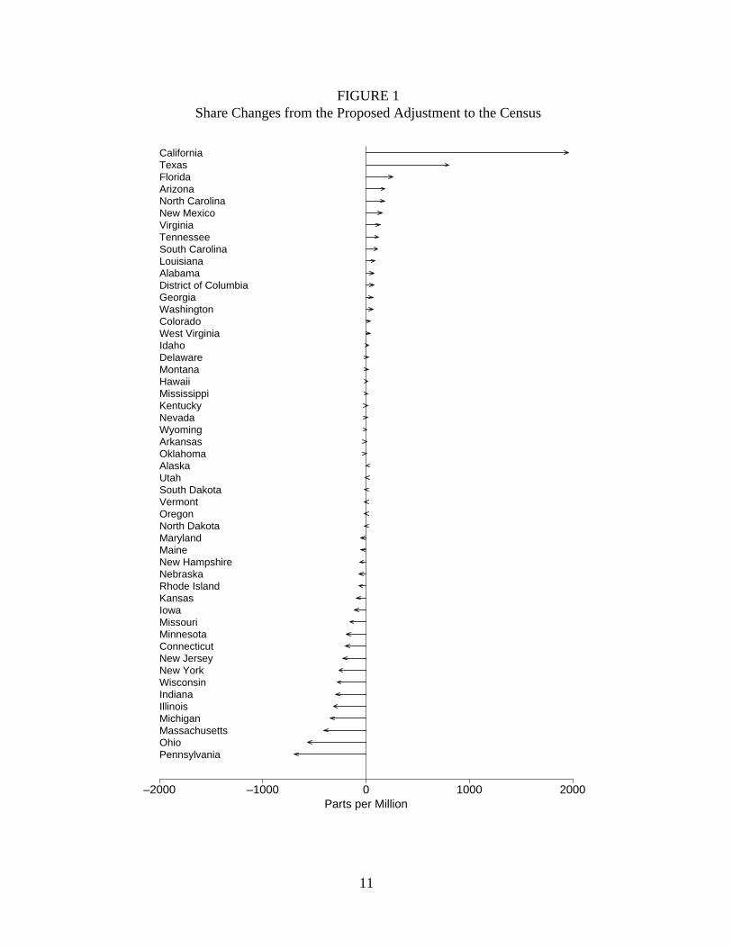
Figure 1 shows the changes in state shares that would have been produced by census adjustmentin 1990, sorted by the size of the change.42 The adjusted share for a state is its adjusted count, dividedby the total adjusted count for the whole country; likewise, the census share is the census count,divided by the census count for the whole country. (The adjustment is the one considered bythe Secretary of Commerce as of July 1991.) The share of California increases from .119658 to.121617, that is, by.121617− .119658= .001959, or 1,959/1,000,000. The length of the arrowto the right of California is 1,959 parts per million. California would have been the biggest gainerfrom adjustment. Arrows to the left correspond to losing population share. Pennsylvania’s sharewould have decreased from .047773 to .047078; the loss is.047773− .047078= .000695, or 695parts per million. That is the biggest loss. (Oddly, Pennsylvania supported adjustment in 1990;

10

FIGURE 1Share Changes from the Proposed Adjustment to the Census

CaliforniaTexasFloridaArizonaNorth CarolinaNew MexicoVirginiaTennesseeSouth CarolinaLouisianaAlabamaDistrict of ColumbiaGeorgiaWashingtonColoradoWest VirginiaIdahoDelawareMontanaHawaiiMississippiKentuckyNevadaWyomingArkansasOklahomaAlaskaUtahSouth DakotaVermontOregonNorth DakotaMarylandMaineNew HampshireNebraskaRhode IslandKansasIowaMissouriMinnesotaConnecticutNew JerseyNew YorkWisconsinIndianaIllinoisMichiganMassachusettsOhioPennsylvania

200010000–1000–2000Parts per Million

11

so did New York and New Jersey.) For many of the states, the adjustment would have been lessthan 30 parts per million: the arrowhead overlaps the vertical line marking no change in populationshare.

There are two noteworthy features. First, the share changes are tiny: the median size of thechange is 75 parts per million. Second, the Northeastern and Midwestern states with large central-city minority populations—like New York, Illinois, Michigan, Massachusetts, and Pennsylvania—would have lost share from adjustment. If adjustment were accurately correcting for racial differ-entials in the undercount, these states would have been expected to gain population share. Oneplausible explanation for the paradox is correlation bias.

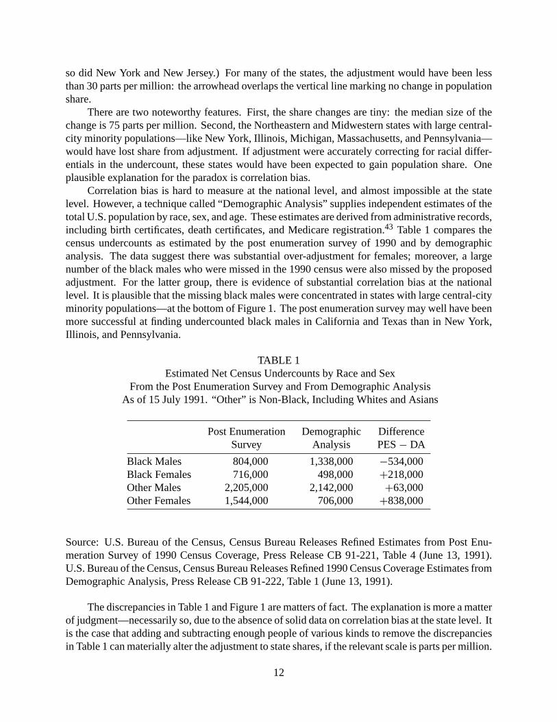
Correlation bias is hard to measure at the national level, and almost impossible at the statelevel. However, a technique called “Demographic Analysis” supplies independent estimates of thetotal U.S. population by race, sex, and age. These estimates are derived from administrative records,including birth certificates, death certificates, and Medicare registration.43 Table 1 compares thecensus undercounts as estimated by the post enumeration survey of 1990 and by demographicanalysis. The data suggest there was substantial over-adjustment for females; moreover, a largenumber of the black males who were missed in the 1990 census were also missed by the proposedadjustment. For the latter group, there is evidence of substantial correlation bias at the nationallevel. It is plausible that the missing black males were concentrated in states with large central-cityminority populations—at the bottom of Figure 1. The post enumeration survey may well have beenmore successful at finding undercounted black males in California and Texas than in New York,Illinois, and Pennsylvania.

TABLE 1Estimated Net Census Undercounts by Race and Sex

From the Post Enumeration Survey and From Demographic AnalysisAs of 15 July 1991. “Other” is Non-Black, Including Whites and Asians

Post Enumeration Demographic DifferenceSurvey Analysis PES− DA

Black Males 804,000 1,338,000 −534,000Black Females 716,000 498,000 +218,000Other Males 2,205,000 2,142,000 +63,000Other Females 1,544,000 706,000 +838,000

Source: U.S. Bureau of the Census, Census Bureau Releases Refined Estimates from Post Enu-meration Survey of 1990 Census Coverage, Press Release CB 91-221, Table 4 (June 13, 1991).U.S. Bureau of the Census, Census Bureau Releases Refined 1990 Census Coverage Estimates fromDemographic Analysis, Press Release CB 91-222, Table 1 (June 13, 1991).

The discrepancies in Table 1 and Figure 1 are matters of fact. The explanation is more a matterof judgment—necessarily so, due to the absence of solid data on correlation bias at the state level. Itis the case that adding and subtracting enough people of various kinds to remove the discrepanciesin Table 1 can materially alter the adjustment to state shares, if the relevant scale is parts per million.

12

We conclude that correlation bias is a serious and intractable problem. The bias is serious becauseit can result in adjustments that make state shares worse rather than better. The bias is intractablebecause it cannot be measured at subnational levels.44

VI. HETEROGENEITY

As noted above, the Bureau divides the population into post strata defined by demographicand geographic characteristics: one post stratum might be Hispanic male renters age 30–49 inCalifornia. Sample persons are assigned to post strata on the basis of the fieldwork. The rate ofgross omissions, erroneous enumerations, and the net undercount rate are estimated separately foreach post stratum (Section VIIA). It is the net undercount rate that matters for adjustment.

To adjust small areas (counties, cities,. . . , blocks), the undercount rate in a post stratum isassumed to be constant across geography. In our example, the number of Hispanic male rentersage 30–49 in every single block in California—from the barrios of east Los Angeles to the affluentsuburbs of Marin county and beyond—would be scaled up by the same adjustment factor, whichis computed from sample data for the whole post stratum. This process, of course, is repeated forevery post stratum. The choice of post strata may therefore have a substantial influence on theresults.45 Plainly, the choice of post strata is somewhat subjective. The assumption that undercountrates are constant within post strata is the “homogeneity assumption,” and failures are termed“heterogeneity.” Ordinarily, samples are used to extrapolate upwards, from the part to the whole.Census adjustment extrapolates sideways, from 60,000 sample blocks to each and every one of 5million inhabited blocks in the U.S. That is why the homogeneity assumption is needed.

In July 1991, the Bureau proposed to use 1,392 post strata. The Bureau later consideredadjusting the census as a base for the post-censal estimates (Section IVE), using 357 post strata. Witheither post stratification, there was considerable residual heterogeneity.46 This added appreciablyto the uncertainties about adjustments for state and sub-state areas, and significantly complicatedthe task of comparing the accuracy of the census to that of adjustment.47

The Bureau has not finalized its post stratification for 2000.48 In the plan reviewed by thecourts, post strata would not have crossed state lines: thus, each state would be adjusted only usingdata collected within that state. This is an improvement over 1990, because homogeneity of poststrata that cross state lines is not assumed. There is a cross-classification within each state (andD.C.) by six race-ethnicity groups, seven age-sex groups, and two “tenure” groups—owners andrenters. Post strata can be formed from these 6× 7 × 2 = 84 categories by collapsing cells withsmall sample sizes, although that part of the process was not fully defined. These post strata do nottake into account area of residence—whether respondents live in major metropolitan areas, suburbs,or rural areas. For that reason, heterogeneity within states may be even more of a problem in 2000than it was in 1990. In the current plan, post strata will cross state lines (Section XI).

VII. DUAL SYSTEM ESTIMATION

VII A. Weights

We turn now to estimation. Each person in the PES is assigned a “sample weight.” If theBureau sampled 1 person in 100, each sample person would stand for 100 in the population, and

13

have a sample weight of 100. The actual sampling plan is more complex, so different people havedifferent weights. Basically, the weight is the inverse of the selection probability, with adjustmentsfor non-response. Each gross omission or erroneous enumeration detected in the sample is weightedup in the estimation process.

To estimate the total number of gross omissions in a post stratum, one simply adds the weightsof all PES respondents who were identified as (i) gross omissions and (ii) in the relevant post stratum.To a first approximation, the estimated undercount in a post stratum is the difference between theestimated numbers of gross omissions and erroneous enumerations. Details are postponed to theAppendix. The “raw adjustment factor” for a post stratum is the ratio of its estimated populationto the census count: when multiplied by this factor, the census count for a post stratum equals theestimated true count. Typically, adjustment factors exceed 1: most post strata are estimated to haveundercounts. However, many adjustment factors are less than 1. These post strata are estimated tohave been overcounted. In 1990, about 70% of the adjustment factors exceeded 1 and 30% werebelow 1.

Use of sample weights is of course quite standard, but not free of problems in the adjustmentcontext. For one thing, mistakes in fieldwork are magnified by the weights. For another thing,the weights may themselves be adjusted at various stages of the process, for reasons that are notentirely compelling—and the impact of such changes can be striking. Thus, a decision to revisethe weights of two block clusters out of the 5,300 in the 1990 post enumeration survey subtracted654,000 people from the adjusted count.49

VII B. Smoothing in 1990

In 1990, the raw adjustment factors had unacceptable levels of sampling error. As noted above,the Bureau tried to reduce sampling error by means of smoothing. This was done separately infour geographical regions—Northeast, Midwest, South, and West. In the Northeast, for instance,there were 300 post strata. The Bureau was using a “hierarchical linear model,” with two equations(reported in the Appendix). The first equation states an assumption, that the raw adjustment factorfor a post stratum is an unbiased estimate of the true factor. The second equation in the modelstates another assumption, that the true adjustment factors are linearly related to certain covariates,with additive random errors. The “smoothed adjustment factors” are obtained by averaging theraw factors with values predicted from an auxiliary regression model. The weights in the averagedepend critically on the variances of the raw factors. These variances are initially estimated fromthe data,50 but are then “pre-smoothed,” that is, replaced by values predicted from yet anotherregression model.

The detailed structure of the models seems arbitrary, and details had major impacts. Forinstance, the proposed adjustment in 1990 would have shifted population share from the Northeastand Midwest to the South and West; pre-smoothing and benchmarking account for 1/3 of the shift.51

Moreover, the estimated variances in the smoothed adjustment factors depend quite strongly on theassumptions in the model. If these assumptions are violated, real variances may be much larger thanthe estimated variances. When model outputs were taken at face value, smoothing seemed to reducevariances by a factor of about 2. However, simulation studies and sensitivity analysis suggest thatestimated variances were too small by a factor of 2 or 3: if anything, smoothing increased variance.52

Pre-smoothing accounted for nearly half of the 5.3 million estimated undercount.53

14

VII C. Smoothing in 2000

The Bureau planned to smooth the adjustment factors in Census 2000 by means of a log linearmodel, in order to reduce variance.54 (Although the ICM would have been 5 times larger than thePES of 1990, there would have been 2 or 3 times as many post strata; thus, sampling error is still aproblem.) There are strong similarities between the log linear model for 2000 and the linear modelfor 1990, although the one for 2000 may be simpler and therefore more robust. The benchmarkingwill certainly be more extensive. However, the basic issue remains the same: a reduction in varianceis likely to be accompanied by some increase in bias, and the tradeoff is extraordinarily hard toassess.55

VIII. LOSS FUNCTION ANALYSIS

In brief, “loss function analysis” attempts to make unbiased estimates of the risk in the censusand the adjustment. Various loss functions can be considered, and different levels of geography.We focus here on total squared error in population shares for the 50 states and D.C. The object is toestimate “census risk− adjustment risk:” risk is squared error, averaged over possible realizationsof the PES and the Evaluation Followup (Section IVA). Using the Bureau’s assumptions, this riskdifference is estimated as 667, with a standard error of 281. With other assumptions that are perhapsmore realistic, the estimate becomes−250, with a standard error of 821; units are parts per 100million, positive values favoring adjustment and negative values favoring the census. Even at thestate level, the case for adjusting the 1990 census was shaky at best: there was a strong likelihoodthat adjustment would have put in more error than it took out, and conclusions depend heavily onassumptions. A technical discussion is postponed to the Appendix.

IX. SAMPLING FOR NON-RESPONSE

IX A. SNRFU

We now turn to “SNRFU,” or Sample-based Non-Response Followup. This was the componentof the plan for 2000 ruled out by the courts (Section II). Non-response followup in the census has inthe past been done on a 100% basis. In the bulk of the country, forms are mailed out to all identifiedhousing units. If there is no response, interviewers come knocking on the door. In 2000, the Bureauplanned to follow up only a sample of non-respondents, within each tract. If, for instance, a tracthas 2,000 housing units and 1,200 return their census form by mail, there are 800 non-respondingunits. The Bureau would then have sampled 600 out of these 800 units, sending interviewers onlyto the sample units. A separate sample would be drawn from the forms returned by the Post Officeas undeliverable. Additional housing units would be imputed into the census using responses fromthe two samples.

A “tract” is a unit of census geography, containing on average something like 100 blocks,2,000 housing units, and 5,000 people. The idea is to obtain responses from 90% of the housingunits in each tract. In our example, 1,200+ 600 = 1,800, which is 90% of the assumed total of2,000; if the mail-back rate in a tract is above 85%, the sampling rate is held at 1 in 3. Sample datamay for instance suggest adding a certain number of households of a given type; some householdswould be selected from enumerated households of that type and added to the census.

15

There is some opinion that sampling improves accuracy since interviewers can be better trainedand supervised. Given the proposed sampling rates, this advantage cannot be substantial. Samplingseems inherently more complex than a census, and past experience shows that sample surveys haveworse coverage than the census. Of course, sampling for non-response in Census 2000 may not bedirectly comparable to past surveys. Coverage can be explained this way. As noted above, eachperson in a sample gets a sample weight: this could, for instance, be the inverse of the probability ofdrawing that person into the sample. Based on sample data, one can then estimate the total numberof persons in the population by adding up the weights of the sample persons. “Coverage” is theratio of this estimated number to the true number. Likewise, the coverage of the census is the ratioof the census population to its (estimated) true value.

The Current Population Survey is a well-established, well-run sample survey; still, it reachesonly about 95% of the census population. Relative to the census, the CPS has a 95% coverage ratio.Black and Hispanic sub-populations have noticeably lower coverage ratios.56 For another example,the post enumeration survey of 1990 had by our reckoning about 98% of the coverage of the census.(The calculation weights the P-sample and E-sample to national totals.) Of course, the census datawere in some cases problematic—but so were the post enumeration survey data. It is by no meansobvious that SNRFU will reduce differential undercounts.

IX B. How Does Sampling for Non-Response Interact with the ICM?

The essential task of the ICM is to match records against the census. That conflicts withsampling for non-response, because ICM respondents may be in households that did not return acensus form and were not selected for followup. To solve this problem, the Bureau proposed todo 100% followup in the ICM sample blocks. The plan for Census 2000 that was rejected by thecourts therefore involved at least three kinds of sampling and three kinds of fieldwork.

The three kinds of sampling:

(i) sampling in the ICM;(ii) sample-based followup for census non-response;

(iii) sampling housing units with undeliverable census forms.

The three kinds of fieldwork:

(i) the ICM;(ii) 100% followup for census non-response in the ICM sample blocks;

(iii) sample followup for census non-response in the rest of the country.

Other assumptions would be needed here: (i) census coverage is the same whether non-responsefollowup is done on a sample basis or a 100% basis; and, (ii) residents of the ICM sample blocks donot change their behavior as a result of being interviewed more than once. Failure of these assump-tions may be termed “contamination error.” The magnitude of contamination error is unknown. Atest census may provide evidence showing that contamination error is modest. However, power islimited and the real census may be somewhat different.57 One other feature of the design reviewedby the courts is worth considering here: the ICM could not have detected any non-sampling errorsin SNRFU, because the ICM would not—by design—examine any blocks where non-responsefollowup is done on a sample basis.

16

X. OTHER ARGUMENTS

In this section, we review some additional arguments for sampling and adjustment.58

Everything is relative: the census is imperfect, and survey data are of better quality thancensus data.The imperfection of the census may be granted. However, even if the PES is in someways better than the census, the central question remains open. Are the PES data good enough fortheir intended use? Will proposed adjustments to the census take out more error than they put in?

Sampling saves money and improves accuracy.“Without sampling, costs would increase by atleast $675 million and the final count would be less accurate than the 1990 census.” p. 37. However,sampling 3 households in 4 within each tract cannot have saved very much money. The budgetfor non-response followup is only about $500 million, and the sampling rate is about 3/4, so thesavings may be on the order of $150 to $200 million rather than $675 million. For comparison, thetotal budget is about $4 billion.59

If there was little money to be saved by SNRFU, few gains in accuracy would have resultedfrom putting those savings into improvements in fieldwork. The case that sampling will improveaccuracy must rest therefore on the post enumeration survey and the DSE: “The Census Bureau isconfident in the Dual System Estimation methodology based on its experience implementing DualSystem Estimation and its expertise explaining Dual System Estimation. . . .” p. 32. In our view,however, the DSE failed to improve accuracy in 1980; and it failed again in 1990.60 The crucialquestion is whether the DSE will improve accuracy in 2000.

The argument from authority.The Bureau’s plans have been approved by “three separatepanels” of the National Academy of Sciences, six Census Advisory Committees, and “publicmeetings. . . in thirty-one cities across the country.” pp. 7, 9. The National Academy reportsprovide little analytic detail supporting adjustment. Nor are they quite as supportive of samplingas the Bureau makes out: “If sampling for NRFU frees resources for taking steps to reduce othersources of error in the final results, it may produce a more accurate census by some measures.”Steffey and Bradburn, supra note 57, at 101. This is hardly a ringing endorsement.

Sampling is scientific.“Scientists understand that sampling has known, objective propertiesthat are preferable to the certainty of missing several million individuals using traditional enumer-ation methods alone. . . . the issue is not whether to ‘sample’ but whether to sample scientifically.”pp. ii, 23. Presumably, the census is an unscientific “sample” because it is not an exact count ofthe population; the “known, objective properties” of a scientific sample must refer to the possibilityof quantifying sampling error. However, the argument is diversionary as well as murky. The realproblem is non-sampling error. The PES will suffer from non-sampling error, which will be as hardto quantify as the errors in the census.

Adjustment will correct the differential undercount for national race and ethnic groups, andmay improve the accuracy of state and local shares.We think this was the best argument foradjustment in 1990, although it was seldom made explicit. However, it is not an argument forthe post enumeration survey and the DSE, because there is a much simpler way to correct thenational undercount. Census figures could be scaled up to match the demographic analysis totalsfor subgroups of the national population defined by age, sex and race (Section V). The people ina demographic group who are thought to be missing from the census would be added back, inproportion to the ones who are counted—state by state, block by block. Currently, demographicanalysis does not account for ethnicity, but the method could be adapted for that purpose. Scaling istransparent, so there is little opportunity for major error. Changes in state and local-area population

17

shares may go in the right direction and will in any event be small. Despite the flaws in demographicanalysis and the heterogeneity of undercount rates, we do not see much likelihood of demonstratingthat the DSE will be more accurate than scaling. On the contrary, the DSE may do worse becauseof some hidden breakdown in the operation.

XI. THE MODIFIED PLAN FOR CENSUS 2000

In response to the Supreme Court’s decision, the Executive Branch is planning a two-trackcensus. The apportionment numbers will be based on a headcount. For other purposes, censuscounts will be adjusted using a revised version of the ICM, to be called ACE (Accuracy andCoverage Evaluation Survey). The sample size will be about 40% of the planned size for ICM,that is, about double the size of the 1990 PES. Post strata are not yet defined, but will almostcertainly cross state lines.61 Plans for sample-based non-response followup have been dropped, sothe complicated interactions with ICM fieldwork will no longer be a problem (Section IX). In otherrespects, the new poposal seems very like the one described here, and very like the 1990 plan. Themajor differences we see between plans for 2000 and 1990 are now as follows:

(i) Counts will be adjusted using ACE, for purposes other than apportionment of congres-sional seats to states. In 1990, there was no adjustment.

(ii) ACE will be almost double the size of the 1990 PES.(iii) Outmovers identified by ACE will be matched to the census; the PES attempted to identify

and match inmovers (Section IVD).(iv) Census fieldwork will be curtailed to make time for ACE fieldwork.(v) Census forms will be widely distributed through the “Be Counted” program, as well as

being mailed or delivered to all addresses in the Master Address File. This increases therisk of duplicate enumerations.

XII. SUMMARY AND CONCLUSION

One of the oft-stated goals for Census 2000 is “Keep It Simple.”62 However, adjustment addslayer upon layer of complexity to an already complex census. Consequently, the results are highlydependent on many somewhat arbitrary technical decisions. Mistakes are almost inevitable, veryhard to detect, and have profound consequences. Examples from 1990 are sobering:

(i) A computer coding error added a million people to the adjusted count (Section IVE).(ii) In total, about 3.0 to 4.2 million out of the estimated 5.3 million undercount resulted from

errors in the PES rather than census errors (Section IVA).(iii) The treatment of the Q-class by the imputation model subtracted 400,000 to 900,000

people from the adjusted count (Section IVC).(iv) A decision to revise the weights of two block clusters out of the 5,300 in the 1990 PES

subtracted 654,000 people from the adjusted count (Section VIIA).(v) The decision to pre-smooth estimated variances added 2.5 million people to the adjusted

count (Section VIIB).

The specific sources of instability discovered in 1990 may well be avoided in 2000. But the lesson isthat the kinds of methods proposed to fix the census are quite dependent on many somewhat arbitrary

18

technical decisions, and inherently vulnerable to error. Furthermore, the statistical assumptionsbehind the adjustment methodology are rather shaky. The homogeneity assumption is one example(Section V); the imputation and smoothing models can also be mentioned (Sections IVC, VIIC);and the list does not end there. If the PES of 2000—like the PES of 1990 before it—puts in moreerror than it takes out, Census 2000 will be at considerable risk.

APPENDIX

The Dual System Estimator

The formula for the raw dual system estimator (DSE) is

DSE= Cen− II

M/Np

×[1 − EE

Ne

].

In this formula, DSE is the dual system estimate of the population in a post stratum; Cen is the censuscount;II is the number of persons imputed into the census count;M is the estimated total numberof matches obtained by weighting up sample matches;Np is the estimated population obtained byweighting up P-sample counts;EE is the estimated number of erroneous enumerations; andNe

is the estimated population obtained by weighting up E-sample counts. The formula is appliedseparately to each post stratum.

The “match rate”M/Np appears in the denominator of the DSE. Intuitively, the complementof the match rate estimates the gross omissions rate in the census. Likewise,EE/Ne estimatesthe rate of erroneous enumerations in the census. The object of the post enumeration survey is toestimate these fractions. Cen andII come from census records. Some persons besides theII ’s arecounted in the census without enough detail for matching; such persons are classified as erroneousenumerations, as are persons who have been counted more than once.63

The Smoothing Model

We use the Northeast as an example. There were 300 post strata, which we index byi. Let γi

be the “true” adjustment factor for post stratumi, andYi the “raw” adjustment factor derived fromthe DSE. The Bureau was using a hierarchical linear model. The first equation in the model statesan assumption, that the raw adjustment factor is an unbiased estimate of the true factor:

Yi = γi + δi,

whereδi is a random error term.The second equation in the model states another assumption, that the true adjustment factors

are linearly related to certain covariates, with additive random errors:

γ = Xα + ε.

Here,α is a vector of unknown parameters andX is a matrix of covariates computed from censusdata; theith row of X describes post stratumi. Again, ε is a vector of random errors, assumed

19

independent ofδ, with E(ε) = 0 and cov(ε) = σ 2I , whereσ 2 is another parameter to be estimated.Random errors are assumed to be multivariate normal.

Let δ be the vector whoseith component isδi , and letK = cov(δ), whereK is a 300× 300matrix that is estimated from the data by the jackknife. After estimation, variances are “pre-smoothed,” that is, replaced by fitted values computed from some auxiliary regression model. Callthe resulting estimateK. The “smoothed” adjustment factorsγ are obtained by projecting the rawadjustment factorsY toward a hyper-plane defined byX; direction and distance are determined byK. Thus, the algorithm depends strongly on estimated variances.

To implement the smoothing model, the Bureau drew up a list of admissible covariates. Fromthis list, some initial versionX0 was chosen forX. Thenσ 2 andα are estimated by maximumlikelihood, and a new version ofX is chosen by a “best subsets” routine from the list of admissiblecovariates, and there is iteration to convergence.64 In the Northeast, for instance, the algorithmchose 18 covariates out of a possible 32.

Write X for the “final” version of the design matrix. Denote the MLE forσ 2 by σ 2. Let PX

be the OLS projection matrix,PX = X(X′X)−1X′. Define the 300× 300 matrix0 as follows:0−1 = K−1 + σ−2(I − PX). The vector of smoothed adjustment factors could be computed asγ = 0K−1Y , with covariances estimated ascov(γ − γ ) = 0. In 1990, however, the Bureau“benchmarked”γ so the total population in each of the four regions was unaffected by smoothing.This necessitated a more complex formula for the covariances ofγ . The formula allowed foruncertainty inσ 2. No allowance was made for uncertainty inK, or in the choice ofX. Noallowance was made for specification error.65

Loss Function Analysis

Index the areas byk = 1, . . . , 51, corresponding to the 50 states and D.C. Letµk be the errorin the census population share for areak. Let Xk be the production dual system estimate forµk,derived from the post enumeration survey and the smoothing model. The bias inXk is denotedβk;this is estimated from evaluation followup data asβk. The Bureau’s model can be stated as follows:X ∼ N(µ + β, G), β ∼ N(β, H), andX is independent ofβ. Here,X, β, andβ are 51-vectorsof share changes;G andH are 51× 51 matrices of rank 50. Shares add to unity, so share changesadd to 0, and one degree of freedom is lost. The smoothing model provided an estimatorG forG, and the Bureau had an estimatorH for H ; these estimators were assumed to be nearly correct.Likewise, the model assumedβ to be an unbiased estimator forβ. We find these assumptions tobe extremely questionable: for example,β is severely biased (Section IV above).

The estimated risk from the census for areak is (Xk − βk)2 − Gkk − Hkk, while the estimated

risk from adjustment isβ2k + Gkk − Hkk. The estimated risk difference is

Rk = (Xk − βk)2 − β2

k − 2Gkk.

The covariance can be computed, ignoring the variability inG, as

cov(Ri , Rj ) = 4µiµjGij + 2G2ij + 4E(XiXj )Hij .

The displayed covariance can be estimated from sample data as

Cij = 4(Xi − βi )(Xj − βj )Gij − 2G2ij − 4Gij Hij + 4XiXj Hij .

20

Thus, we have unbiased estimates—given the model, and given that

E(G) = G, E(H ) = H.

Let ERD be the estimated risk difference, summed over all 51 areas: ERD= ∑k Rk. Now

var(ERD) can be estimated as∑

ij Cij . Table 2 shows ERD and var(ERD), computed using theformulas above, under various sets of assumptions. Bias was measured for 13 evaluation poststrata, and allocated by the Bureau to 1,392 post strata. The Bureau’s allocation assumed (i) biaswas proportional to some covariate for post strata within evaluation post strata, and (ii) bias wasconstant across states within post strata. Bias was allocated down, then reaggregated to the 51areas. The evaluation followup sample was about 7% of the size of the post enumeration survey;there was no smoothing (factor of 2 reduction in apparent variance). Trace(H ) should thereforehave been around

1

.07× 2 × trace(G).

Instead, on the Bureau’s reckoning, trace(H ) turned out to be around.33× trace(G). We concludethatH is off by a factor of around

1

.07× 2 × 1

.33= 84.

The explanation: the Bureau’s allocation scheme converted variance inβ to bias, and their modelassumed that bias inβ vanishes.

TABLE 2Impact of Allocation Schemes for State-Level Biases

Correction of Final Variances and Estimated Variances of Bias EstimatesERD= Census Risk− Adjustment Risk

The “SE” Column Gives the Estimated Standard Error of ERDin the Various Scenarios. Units are parts per 100 million

Allocation G H ERD SE

PRODSE 1 1 667 281

PRODSE 1 50 667 890

PRODSE 2 1 542 371

PRODSE 2 50 542 885

.25× undercount 1 1 193 199

.50× undercount 1 1 −125 156

.50× undercount 1 50 −125 859

.50× undercount 2 1 −250 169

.50× undercount 2 50 −250 821

21

The matrixG is too small as well, by a factor of 2 to 3, as discussed in Section VIIB. Further-more, measured biases in the post enumeration survey—response errors, matching errors, errorsin the imputations for missing data, the coding error, and so forth—amount to well over half theestimated undercount, as reported in Section IIIA. The first line in Table 2 does the loss func-tion analysis on the Bureau’s assumptions. The other lines show what happens when the varianceestimates are corrected, and the bias allocations are revised.66

Table 2 may in some respects understate the problems with loss function analysis. For instance,heterogeneity is probably larger than all the other errors put together, and heterogeneity is not takeninto account in Table 2; there is no allowance for bias in the imputations; and the Bureau’s schemefor allocating biases to states violates the assumption thatβ should be independent ofX. (Ours doestoo.) We think the last line in the table is the most plausible.67 Taken as a whole, the table showsthat loss function analysis depends very strongly on the assumptions going into the evaluation: theavailable data do not decide the issue. We suspect that methods like loss function analysis will beused to justify the ICM in Census 2000.

AFFILIATIONS

L.D. Brown, Department of Statistics, University of Pennsylvania, Philadelphia; M.L. Eaton,Department of Theoretical Statistics, University of Minnesota, Minneapolis; D.A. Freedman,K.W. Wachter, Department of Statistics, U.C. Berkeley; R.A. Olshen, Division of Biostatistics,Stanford University; S.P. Klein, RAND Corporation, Santa Monica, M.T. Wells, Department ofSocial Statistics, Cornell University, D. Ylvisaker, Statistics Department, UCLA.

ACKNOWLEDGMENTS

We thank the Donner Foundation for its support (DAF, KWW, MTW, and DY). We also thankour editor, David Kaye, for his help, along with Mike Finkelstein and Philip Stark. DAF and KWWtestified for defendants in the census litigation of 1980 and 1990; more recently, they have consultedfor the Freshpond Research Institute on census adjustment.

FOOTNOTES

1. For conflicting views on proposed adjustments to the 1990 census, see the exchanges of papers at9 Stat. Sci. 458 (1994), 18 Survey Methodology No. 1 (1992), 88 J. Am. Stat. Ass’n 1044 (1993),and 34 Jurimetrics J. 65 (1993).

2. Title 13 of the U.S. Code.

3. In Wisconsin v. City of New York, 116 S.Ct. 1096, the Supreme Court resolved the conflictamong the circuits over the legal standard governing claims that adjustment is compelled by statuteor constitution. Compare City of New York v. United States Dep’t of Commerce, 34 F.3d 1114(2d Cir. 1994) (equal protection clause requires government to show compelling interest that couldjustify Secretary of Commerce’s refusal to adjust 1990 census), rev’d sub nom. Wisconsin v. City ofNew York with City of Detroit v. Franklin, 4 F.3d 1367 (6th Cir. 1993) (neither the statutes nor theconstitution requires adjustment), cert. denied sub nom. City of Detroit v. Brown, 510 U.S. 1176(1994); Tucker v. United States Dep’t of Commerce, 958 F.2d 1411 (7th Cir.) (issue is not justiciable),cert. denied, 506 U.S. 953 (1992). In Wisconsin, the Supreme Court unanimously determined thatthe exacting requirements of the equal protection clause, as explicated in congressional redistricting

22

and state reapportionment cases, do not “translate into a requirement that the Federal Governmentconduct a census that is as accurate as possible. . . .” 116 S.Ct. at 1099–1100. The Court thereforeapplied a much less demanding standard to the Secretary’s decision.

“In 1990, the Census Bureau made an extraordinary effort to conduct an accurate enumeration,and was successful in counting 98.4% of the population. . . . The Secretary then had to considerwhether to adjust the census using statistical data derived from the PES. He based his decisionnot to adjust the census upon three determinations. First, he held that in light of the constitutionalpurpose of the census, its distributive accuracy was more important than its numerical accuracy.Second, he determined that the unadjusted census data would be considered the most distributivelyaccurate absent a showing to the contrary. And finally, after reviewing the results of the PES in thelight of extensive research and the recommendations of his advisers, the Secretary found that thePES-based adjustment would not improve distributive accuracy. Each of these three determinationsis well within the bounds of the Secretary’s constitutional discretion. . . . Moreover, even those whorecommended in favor of adjustment recognized that their conclusion was not compelled by theevidence. . . . Therefore, and because we find the Secretary’s. . . prior determinations. . . to beentirely reasonable, we conclude that his decision not to adjust the 1990 census was ‘consonantwith . . . the text and history of the Constitution. . . .’” 116 S.Ct. at 1101, 1103.

Concluding that the government had shown “a reasonable relationship” between the decision not tomake post hoc adjustments and “the accomplishment of an actual enumeration of the population,keeping in mind the constitutional purpose of the census. . . . to determine the apportionment ofthe Representatives among the States,” the Court held that the decision satisfied the Constitution.Indeed, having rejected the argument that the constitution compelled statistical adjustment, theCourt noted that the constitution might prohibit such adjustment. 116 S.Ct. at 1109 & n.9. Thisfootnote is adapted from D.H. Kaye and D.A. Freedman, Statistical Proof, in Modern ScientificEvidence, Vol. I, 83, 92 (D.L. Faigman, D.H. Kaye, M.J. Saks, J. Saunders, eds., 1997). There isfurther discussion in D.A. Freedman and K.W. Wachter, Planning for the Census in the Year 2000,20 Eval. Rev. 355 (1996).

4. Pub.L. 105-18, tit. VIII, 111 Stat. 158, 217 (1997). Sections 209 and 210 of the Departmentsof Commerce, Justice, and State, the Judiciary, and Related Agencies Appropriations Act, 1998,Pub.L. 105-119, 111 Stat. 2440, 2480-87 (1997). For the Bureau’s report, see infra note 32.

5. 11 F.Supp.2d 76 (D.D.C. 1998) at 87, 90–91.

6. Id. at 89.

7. Id. at 94.

8. 13 U.S.C. §195.

9. 13 U.S.C. §141(a).

10. 11 F.Supp.2d at 103.

11. Id. at 104.

12. 11 F.Supp.2d at 104.

13. Order and Judgment at 2.

14. 19 F.Supp.2d 543 (E.D.Va. 1998).

15. Id. at 548.

23

16. Id. at 552–53.

17. Id. at 553.

18. Dep’t. of Commerce et al. v. U.S. House of Representatives et al. and Clinton et al. v. Glavin etal. Slip Op. January 25, 1999.

19. Id. at 9.

20. Id. at 11.

21. Id. at 13.

22. Id. at 14.

23. Id. at 16.

24. Id. at 16.

25. Id. at 20.

26. Id. at 21.

27. Id. at 22.

28. Id. at 26.

29. Pub.L. 105-119 §209(j).

30. We computed the figures from the Bureau’s Advisory Use File. There is substantial overlapbetween the 19 million and the 13 million, namely, persons whose addresses were geocoded tothe wrong block (Section IVB). Other observers quote different numbers; see, for instance, S.E.Fienberg, The New York City Census Adjustment Trial: Witness for the Plaintiffs, 34 JurimetricsJ. 65, 70 (1993). According to the GAO, “The Bureau of the Census estimated that about 6 millionpersons were counted twice in the 1990 Census, while 10 million were missed.” U.S. GeneralAccounting Office, 2000 Census: Progress Made on Design, But Risks Remain, Washington, D.C.,at 7, 56 (1997). These figures are widely quoted. We believe they apply to the revised PES (SectionIVE), but cannot verify them; indeed, they are somewhat inconsistent with other data published bythe Bureau.

31. The ICM would have had a sample of about 1.7 million people; ACE is likely to have a sampleof about 700,000; the 1990 PES had a sample of about 380,000.

32. U.S. Bureau of the Census, Report to Congress—The Plan for Census 2000, Bureau of theCensus, Washington, D.C. at 21–22, 36 (1997).

33. K. Wolter, Comment, 1 Stat. Sci. 24, 26 (1986)

34. The estimate of 3.0 million can be derived from data in U.S. Bureau of the Census, Decisionof the Director of the Bureau of the Census on Whether to Use Information from the 1990 Post-Enumeration Survey (PES) to Adjust the Base for the Intercensal Population Estimates Producedby the Bureau of the Census, 58 Federal Register 69, 75 (January 4, 1993). The figure of 4.2 millionis reported by L. Breiman, The 1991 Census Adjustment: Undercount or Bad Data? 9 Stat. Sci. 458,471 (1994). There is further discussion in D.A. Freedman and K.W. Wachter, Rejoinder, 9 Stat. Sci.527, 531, 535–36 (1994).

35. J. E. Farber, R. E. Fay, and E. J. Schindler, The statistical methodology of Census 2000, Technicalreport, Bureau of the Census, Washington, D.C. (1998) at 15–16.

36. Breiman, supra note 34, at 473–4.

24

37. The Bureau seemed initially to believe that the imputation models used in 1990 were robust andunbiased. Undercount Steering Committee, Technical Assessment of the Accuracy of Unadjustedversus Adjusted 1990 Census Counts, at 10; reprinted in U.S. Department of Commerce, Office ofthe Secretary, Decision on Whether or Not a Statistical Adjustment of the 1990 Decennial Censusof Population Should Be Made for Coverage Deficiencies Resulting in an Overcount or Undercountof the Population, Explanation, three volumes, Washington, D.C., Appendix 4 (1991). Reprinted inpart in 56 Federal Register 33582 (July 22, 1991). M. Mulry and B. Spencer, Accuracy of the 1990Census and Undercount Adjustments, 88 J. Am. Stat. Ass’n 1080, Table 1 (1993). On the otherhand, senior Bureau technical staff later acknowledged the “subjectivity” of model specification,and the difficulty of quantifying the resulting uncertainties; they also agreed that the missing dataproblem is quite intractable because the missingness mechanism is non-ignorable. R.E. Fay andJ.H. Thompson, The 1990 Post Enumeration Survey: Statistical Lessons in Hindsight, Proceedings,Bureau of the Census Annual Research Conference, Bureau of the Census, Washington, D.C. 71,76 (1993). There is discussion of the 1990 imputation model by T.R. Belin, G.J. Diffendal, S.Mack, D.R. Rubin, J.L. Schafer, and A.M. Zaslavksy, Hierarchical Logistic Regression Models forImputation of Unresolved Enumeration Status in Undercount Estimation, 88 J. Am. Stat. Ass’n1149. Also see T.R. Belin and J.E. Rolph, Can We Reach Consensus on Census Adjustment, 9 Stat.Sci. 486, 489. But see K.W. Wachter, Comment: Ignoring Nonignorable Effects, 88 J. Am. Stat.Ass’n 1161 (1993), Breiman, supra note 34, Freedman and Wachter, supra note 34, at 531 (whichintroduces the Q-class terminology), 535–36.

38. Breiman, supra note 34, at 471–2.

39. We computed these figures from the Bureau’s Advisory Use File.

40. On the revised adjustment, see U.S. Bureau of the Census, supra note 34. H. Hogan, The 1990Post-Enumeration Survey: Operations and Results, 88 J. Am. Stat. Ass’n 1047, 1053–54 (1993).Fay and Thompson, supra note 37, at 74. Belin and Rolph, supra note 37, at 498. D.A. Freedmanand K.W. Wachter, Heterogeneity and Census Adjustment for the Intercensal Base, 9 Stat. Sci. 476(1994). (In Table 2 of that paper, entries 3 and 4 should be interchanged.) Breiman, supra note 34,at 471.

41. Processing errors in the PES of about 1.7 million are reported by M. Mulry, 1990 Post Enu-meration Survey Evaluation Project P16: Total Error in PES Estimates for Evaluation Post Strata,Bureau of the Census, Washington, D.C., Table 19 (1991). The coding error and the results from theextreme blocks add 1.3 million to this estimate, for a total of 1.7 + 1.3 = 3 million, in agreementwith U.S. Bureau of the Census, supra note 34, at 75. On the Bureau’s figures, the processing errorsleft in the revised PES amount to 1.7 million. Breiman, supra note 34, adds 1.2 million to thisestimate.

42. Shares were computed from data supplied by the Bureau, and may differ slightly from otherpublished results due to rounding.

43. R.E. Fay, J.S. Passel, J.G. Robinson, and C.D. Cowan, The Coverage of the Population in the1980 Census, U.S. Department of Commerce, Government Printing Office (1988). D.A. Freedman,Adjusting the 1990 Census, 252 Science 1233 (1991).

44. Efforts to model the bias at the state level in 1990 were quite unsuccessful, as acknowledged bysenior Bureau technical staff. Fay and Thompson, supra note 37, at 76. For another perspective, seeFienberg, supra note 30, at 75. Also see E.P. Ericksen, S.E. Fienberg and J.B. Kadane, Comment, 9

25

Stat. Sci. 511, 514 (1994). But see K.W. Wachter, The Census Adjustment Trial: An Exchange, 34Jurimetrics J. 107, 110–13 (1993), or Freedman and Wachter, supra note 34, at 533–34. For morecomparisons between the PES and Demographic Analysis, see K. Darga,Sampling and the Census,The AEI Press, Washington, D.C. (1999). For a formal model of correlation bias and heterogeneity,see D.A. Freedman, P.B. Stark, and K.W. Wachter, A model for correlation bias, heterogeneity,and ratio estimator bias in census adjustment, Technical Report 557, Department of Statistics, U.C.Berkeley (1999).

45. H. Woltman, Estimated State Level Adjusted Counts Based on Revised State Groups, Bureauof the Census, Washington, D.C. (1991).

46. Freedman and Wachter, supra note 40.

47. Initially, residual heterogeneity was deemed trivial by the Bureau. The Undercount SteeringCommittee, supra note 37 at 7, was “convinced” that “block parts are homogeneous within poststrata”; they saw “no evidence to indicate there are any serious flaws” in the homogeneity assumptionat the state level; they relied on J. Kim, 1990 PES Evaluation Project P12: Evaluation of SyntheticAssumption,” Bureau of the Census, Washington, D.C. (1991). Later, senior Bureau technical staffacknowledged that residual heterogeneity was appreciable. Fay and Thompson, supra note 37, at81. J. Thompson, ICM Stratification and Post Stratification, Bureau of the Census, Washington,D.C., at 7 (1998).

48. P.J. Waite and H. Hogan, Statistical Methodologies for Census 2000—Decisions, Issues, andPreliminary Results, Prepared for Joint Statistical Meetings, August 13, 1998. Technical Report,Bureau of the Census, Washington, D.C., at 8–9 (1998).

49. H. Hogan, Downweighting Outlier Small Blocks, Memorandum from Howard Hogan to JohnThompson, dated 18 June 1991, Bureau of the Census, Washington, D.C. Hogan, supra note 40, at1050.

50. Variances and covariances were estimated using a statistical technique called the “jackknife.”R.E. Fay, VPLX: Variance Estimates for Complex Samples, Bureau of the Census, Washington,D.C. (1990).

51. D.A. Freedman, K.W. Wachter, D. Coster, R. Cutler, and S. Klein, Adjusting the Census of1990: The Smoothing Model, 17 Eval. Rev. 371 (1993).

52. See R.E. Fay, Inferences for Small Domain Estimates from the 1990 Post Enumeration Survey,Bureau of the Census, Washington, D.C. (1992). Also see Freedman et al. supra note 51. But seeJ.E. Rolph, The Census Adjustment Trial: Reflections of a Witness for the Plaintiffs, 34 JurimetricsJ. 85 (1993).

53. E.P. Ericksen and J.W. Tukey, Letter dated 11 July 1991, reprinted in U.S. Department ofCommerce, supra note 37, appendix 16. Freedman and Wachter, supra note 3, has further discussion;also see Fay and Thompson, supra note 37, at 83, Freedman et al. supra note 51.

54. Waite and Hogan, supra note 48.

55. Thompson, supra note 47, at 7.

56. U.S. Bureau of the Census, Money Income of Households, Families and Persons in the UnitedStates: 1992, Series P-60, Washington, D.C., Table D-2 (1993).

26

57. Freedman and Wachter, supra note 3. Also see D.L. Steffey and N.M. Bradburn, editors, CountingPeople in the Information Age, National Academy Press, Washington, D.C., at 115 (1994).

58. Unless otherwise noted, quotations are from U.S. Bureau of the Census, supra note 32.

59. U.S. General Accounting Office, 2000 Census: Preparations for Dress Rehearsal Leave ManyUnanswered Questions, Washington, D.C., at 18, 38 (1998). U.S. Bureau of the Census, The Planfor Census 2000, Revised and Reissued February 28, 1996, Washington, D.C. at V-6 (1996). Thearithmetic behind our estimate: if the cost of non-response followup without sampling is $667million, the cost with sampling at the rate of 3 in 4 is roughly 0.75 × $667

.= $500 million; and$667 − $500= $167 million.

It should further be noted that the ICM would cost in the neighborhood of $500 million. In thecensus context, sampling may not be cost effective.

60. On the 1980 census, see Fay et al. supra note 43; also see D.A. Freedman and W.C. Navidi,Regression Models for Adjusting the 1980 Census, 1 Stat. Sci. 1 (1986). D.A. Freedman and W.C.Navidi, Should We Have Adjusted the U.S. Census of 1980? 18 Survey Methodology 3 (1992).

61. U.S. Bureau of the Census, Updated Summary: Census 2000 Operational Plan, Bureau ofthe Census, Washington, D.C. (1999). D. Kostanich, R. Griffin, D. Fenstermaker, Accuracy andcoverage evaluation survey, Prepared for the March 19, 1999 meeting of the National Academyof Science panel to review the 2000 census, Bureau of the Census, Washington, D.C. (1999). Poststrata may be defined in part by 9 “census divisions:” for instance, the Pacific Division comprisesCalifornia, Oregon, Washington, Hawaii, and Alaska. A typical post stratum might then consist ofHispanic male renters age 30–49 living in the Pacific Division.

62. See, for instance, U.S. Bureau of the Census, Census 2000 Operational Plan, Bureau of theCensus, Washington, D.C., at I-3 (1998).

63. The formula discussed in the text is the one used in 1990. Hogan, supra note 40, at 1050. For the1980 formula, see Fay et al., supra note 43, or Freedman, supra note 43. Apparently, the formulafor 2000 remains to be determined. The logic behind the formula is discussed in Freedman, Stark,and Wachter, supra note 44.

64. For a detailed description of the algorithm, see Hogan, supra note 40, or Freedman et al. supranote 51.

65. This section is adapted from Freedman and Wachter, supra note 3.

66. “PRODSE” is one of the two schemes used by the Bureau to allocate bias from evaluationpost strata to individual post strata: bias was allocated in proportion to the production dual systemestimate of population. Mulry and Spencer, supra note 37, at 1089. This procedure allocates errors toevaluation post strata, then to the post strata themselves, with reaggregation to states. Our allocationoperates directly on share changes for states.β is probably smaller thanµ, which offsets our factorof 84 to some degree.

67. For additional details on loss function analysis and the underlying estimates of error, see Breiman,supra note 34, Freedman and Wachter, supra note 34, Freedman et al. supra note 51, D.A. Freedman,K.W. Wachter, R. Cutler, S. Klein, Adjusting the Census of 1990: Loss Functions, 18 Eval. Rev.243 (1994). The latter papers discuss simulation studies to calibrate the numbers in Table 2. Amongother problems, ERD/SE may have a skewed distribution under the null hypothesis, even ifG

andH are unbiased: much depends on the nuisance parameters in the model. For a view from the

27

architects of the Bureau’s loss function analysis, see Mulry and Spencer, supra note 37; that paperdoes not respond to the issues raised here. Responses are given by Belin and Rolph, supra note 37,or Ericksen, Fienberg and Kadane, supra note 44; but also see Fay and Thompson, supra note 37,at 77–83, Breiman, supra note 34, at 521–27, Freedman and Wachter, supra note 34, at 527–37.

Proponents of adjustment often cite A.M. Zaslavsky, Combining Census, Dual System, and Evalu-ation Study Data to Estimate Population Shares, 88 J. Amer. Statist. Assoc. 1092 (1993). However,Zaslavsky’s calculations depend on statistical assumptions that turn out to be wrong. For instance,he assumes that after the census and the PES are done, the Bureau has unbiased estimates for thebiases in the DSE, with a known covariance matrix. In fact, the bias estimates and their estimatedcovariances were themselves severely biased (Section IV). Also see Freedman and Wachter, supranote 34, at 530, 532, showing that loss function analysis does not measure the social costs of errors,but merely provides a statistical summary, which may or may not be useful. This section is adaptedfrom Freedman and Wachter, supra note 3, which has further discussion.

References

Belin, T.R., Diffendal, G.J., Mack, S., Rubin, D.R., Schafer, J.L., and Zaslavksy, A.M. (1993),“Hierarchical Logistic Regression Models for Imputation of Unresolved Enumeration Status inUndercount Estimation,”Journal of the American Statistical Association,88, 1149–66.

Belin, T.R. and Rolph, J.E. (1994). “Can We Reach Consensus on Census Adjustment?”StatisticalScience,9, 486–508 (with discussion).

Breiman, L. (1994), “The 1991 Census Adjustment: Undercount or Bad Data?”Statistical Science,9, 458–75, 521–27 (with discussion).

Darga, K. (1999),Sampling and the Census.The AEI Press, Washington, D.C.

Ericksen, E.P., Fienberg, S.P., and Kadane, J.B. (1994), “Comment,”Statistical Science,9, 511–15.

Ericksen, E.P. and Tukey, J.W. (1991), Letter dated 11 July 1991, reprinted in U.S. Department ofCommerce (1991), appendix 16.

Fay, R.E. (1990), “VPLX: Variance Estimates for Complex Samples,” Bureau of the Census, Wash-ington, D.C.

Fay, R.E. (1992), “Inferences for Small Domain Estimates from the 1990 Post Enumeration Survey,”Bureau of the Census, Washington, D.C.

Fay, R.E., Passel, J.S., Robinson, J.G., and Cowan, C.D. (1988),The Coverage of the Population inthe 1980 Census,U.S. Department of Commerce, Government Printing Office.

Fay, R.E. and Thompson, J.H. (1993), “The 1990 Post Enumeration Survey: Statistical Lessons, inHindsight,”Proceedings, Bureau of the Census Annual Research Conference, Bureau of the Census,Washington, D.C.

Farber, J.E., Fay, R.E., and Schindler, E.J. (1998). “The statistical methodology of Census 2000,”Technical report, Bureau of the Census, Washington, D.C.

Fienberg, S.E. (1993), “The New York City Census Adjustment Trial: Witness for the Plaintiffs,”Jurimetrics,34, 65–83.

Freedman, D. (1991), “Adjusting the 1990 Census,”Science,252, 1233–36.

28

Freedman, D. (1993). “Adjusting the Census of 1990,”Jurimetrics,34, 99–106.

Freedman, D.A., Stark, P.B., and Wachter, K.W. (1999). A model for correlation bias, heterogeneity,and ratio estimator bias in census adjustment, Technical Report, Department of Statistics, U.C.Berkeley.

Freedman, D. and Navidi,W.C. (1986), “Regression Models for Adjusting the 1980 Census,”Sta-tistical Science,1, 1–39.

Freedman, D. and Navidi, W.C. (1992), “Should We Have Adjusted the U.S. Census of 1980?”Survey Methodology,18, 3–74 (with discussion).

Freedman, D. and Wachter, K. (1994), “Heterogeneity and Census Adjustment for the Post-CensalBase,”Statistical Science,9, 476–85, 527–37 (with discussion).

Freedman, D. and Wachter, K. (1996), “Planning for the Census in the Year 2000,”EvaluationReview,20, 355–77.

Freedman, D., Wachter, K., Coster, D., Cutler, R., and Klein, S. (1993), “Adjusting the Census of1990: The Smoothing Model,”Evaluation Review,17, 371–443.

Freedman, D., Wachter, K., Cutler, R., and Klein, S. (1994), “Adjusting the Census of 1990: LossFunctions,”Evaluation Review,18, 243–280.

Hogan, H. (1991), “Downweighting Outlier Small Blocks,” Memorandum from Howard Hogan toJohn Thompson, dated 18 June 1991, Bureau of the Census, Washington, D.C.

Hogan, H. (1993), “The 1990 Post-Enumeration Survey: Operations and Results,”Journal of theAmerican Statistical Association,88, 1047–60.

Kaye, D. and Freedman, D. (1997), “Statistical proof.” InModern Scientific Evidence.D. Faigman,D. Kaye, M. Saks, J. Saunders, editors. West Legal Publishers.

Kim, J. (1991), “1990 PES Evaluation Project P12: Evaluation of Synthetic Assumption,” Bureauof the Census, Washington, D.C.

Kostanich, D., Griffin, R., and Fenstermaker, D. (1999). Accuracy and coverage evaluation survey.Prepared for the March 19, 1999 meeting of the National Academy of Science Panel to Review the2000 census. Bureau of the Census, Washington, D.C.

Mulry, M. (1991). “1990 Post Enumeration Survey Evaluation Project P16: Total Error in PESEstimates for Evaluation Post Strata,” Bureau of the Census, Washington, D.C.

Mulry, M. and Spencer, B. (1993). “Accuracy of the 1990 Census and Undercount Adjustments,”Journal of the American Statistical Association,88, 1080–91.

Rolph, J.E. (1993), “The Census Adjustment Trial: Reflections of a Witness for the Plaintiffs,”Jurimetrics,34, 85–98.

Steffey, D.L. and Bradburn, N.M., editors (1994),Counting People in the Information Age,NationalAcademy Press, Washington, D.C.

Thompson, J. (1998). “ICM Stratification and Post Stratification,” Bureau of the Census, Washing-ton, D.C.

Undercount Steering Committee (1991), “Technical Assessment of the Accuracy of Unadjusted ver-sus Adjusted 1990 Census Counts,” Reprinted in U.S. Department of Commerce (1991), Appendix4.

29

U.S. Bureau of the Census (1991a), “Census Bureau Releases Refined Estimates from Post Enu-meration Survey of 1990 Census Coverage,” Press Release CB 91-221, June 13.

U.S. Bureau of the Census (1991b), “Census Bureau Releases Refined 1990 Census CoverageEstimates from Demographic Analysis,” Press Release CB 91-222, June 13.

U.S. Bureau of the Census (1993a), “Decision of the Director of the Bureau of the Census onWhether to Use Information from the 1990 Post-Enumeration Survey (PES) to Adjust the Base forthe Intercensal Population Estimates Produced by the Bureau of the Census,”Federal Register,58,69–77 (January 4).

U.S. Bureau of the Census (1993b),Money Income of Households, Families and Persons in theUnited States: 1992, Series P-60, Washington, D.C.

U.S. Bureau of the Census (1997),Report to Congress—The Plan for Census 2000,Bureau of theCensus, Washington, D.C.

U.S. Bureau of the Census (1998),Census 2000 Operational Plan,Bureau of the Census, Wash-ington, D.C.

(1999). U.S. Bureau of the Census (1999).Updated Summary: Census 2000 Operational Plan.Washington, D.C.

U.S. Department of Commerce (1991), Office of the Secretary,Decision on Whether or Not aStatistical Adjustment of the 1990 Decennial Census of Population Should Be Made for Cover-age Deficiencies Resulting in an Overcount or Undercount of the Population, Explanation,threevolumes, Washington, D.C., reprinted in part in theFederal Register,56, 33582–33642 (July 22).

U.S. General Accounting Office (1998),2000 Census: Preparations for Dress Rehearsal LeaveMany Unanswered Questions,Washington, D.C.

Wachter, K. (1993), “The Census Adjustment Trial: An Exchange,”Jurimetrics,34, 107–115.

Waite, P.J. and Hogan, H. (1998), “Statistical Methodologies for Census 2000—Decisions, Issues,and Preliminary Results,” Prepared for Joint Statistical Meetings, August 13, 1998. Technical Re-port, Bureau of the Census, Washington, D.C.

Wolter, K. (1986), “Comment,”Statistical Science,1, 24–28.

Woltman, H. (1991), “Estimated State Level Adjusted Counts Based on Revised State Groups,”Bureau of the Census, Washington, D.C.

Zaslavsky, A.M. (1993). “Combining Census, Dual System, and Evaluation Study Data to EstimatePopulation Shares,”Journal of the American Statistical Association,88 1092–1105.

30