STATISTICAL EVALUATION OF VITAL RATES FOR SMALL GROUPS Rita Zemach, Ph.D. and Peter A. Lachenbruch, Ph.D. University of Michigan and University of North Carolina Introduction In recent years much attention has been devoted to the use of statistical indices of health-related characteristics of populations. In particular, records of vital events such as births and deaths have been used to compute rates which serve to compare one population to another, or to monitor changes over time. These vital rates are frequently used as health status indicators for geographic, racial, ethnic, or other groups. Comparisons are made either between different groups at a fixed point in time, or between time points for a particular group. For example, infant, perinatal, or neonatal mortality rates are often used as indices of both health and adequacy of health care. Inferences are made concerning differences in observed rates among groups, or changes in observed rates over time. In many of these studies, little recognition is given to the fact that the observed rate for a given group at a given time is a random variable, and may be regarded as differing by some chance amount from a hypothetical "true" or expected rate. For relatively large population groups---for example, in comparing vital rates of different nations, or in comparing rates of individual states to the U.S. rate---the variance is negligibly small, and observed differences may be taken as true differences. However, if comparisons of rates are to be made among relatively small groups, or among groups of greatly varying size, such as in examining counties within a state, the possibility of large variance components in the observed rates
Transcript
STATISTICAL EVALUATION OF VITAL RATES FOR SMALL GROUPS
Rita Zemach, Ph.D. and Peter A. Lachenbruch, Ph.D.
University of Michigan and University of North Carolina
Introduction
In recent years much attention has been devoted to the use of
statistical indices of health-related characteristics of populations. In
particular, records of vital events such as births and deaths have been used
to compute rates which serve to compare one population to another, or to
monitor changes over time. These vital rates are frequently used as health
status indicators for geographic, racial, ethnic, or other groups.
Comparisons are made either between different groups at a fixed point in
time, or between time points for a particular group. For example, infant,
perinatal, or neonatal mortality rates are often used as indices of both
health and adequacy of health care. Inferences are made concerning
differences in observed rates among groups, or changes in observed rates
over time.
In many of these studies, little recognition is given to the fact that
the observed rate for a given group at a given time is a random variable,
and may be regarded as differing by some chance amount from a hypothetical
"true" or expected rate. For relatively large population groups---for
example, in comparing vital rates of different nations, or in comparing
rates of individual states to the U.S. rate---the variance is negligibly
small, and observed differences may be taken as true differences. However,
if comparisons of rates are to be made among relatively small groups, or
among groups of greatly varying size, such as in examining counties within
a state, the possibility of large variance components in the observed rates
-2-
requires the use of statistical methods in evaluating differences, and
consideration of errors of estimation.
Because of this uncertainty or error inherent in the observed rates,
caution should be used in collecting such data, and in basing actions on
the results. In truth, though they may seem interesting to study, their
information may be quite limited.
One example of a commonly used health status indicator based on vital
records is the infant mortality rate. This paper examines several
statistical techniques for evaluation of infant mortality rates, as applied
to small-group data, focusing on the problem of drawing inferences when the
denominator (number of live births) is only moderately large. The problems
of estimating the true underlying rate, detecting a change in rate over
time, and detecting a difference in rate between two groups are discussed.
The techniques discussed are applied to data from counties in Michigan.
Although the discussion focuses on infant mortality, the techniques may
be applied to any rates.
Statistical Model
It is assumed that the number of infant deaths in a given population
in a fixed time period is a binomial random variable X. A parameter n is
the number of live births, and p is assumed to be the probability of an
infant's death within Qne year. The probability of k infant deaths, given
n live births, is
P[X=k\n] n! k (l_p)n-kk! (n-k)!P
The observed ratio X/n is the maximum likelihood estimate of p and is
proportional to the usual infant mortality rate R (R=(X/n)x(IOOO».
-3-
The binomial assumption implies that there is a constant probability p of
infant death, and that successive deaths are statistically independent
events. Although these assumptions are invalid in particular cases, the
binomial model provides a reasonable and simple statistical basis for
analysis.
In the following discussion rates are expressed sometimes as
proportions and sometimes as rates per 1000. Thus, a rate usually ex-
pressed as 26.3 (per 1000 live births) may be given as a proportion, .0263.
This proportion is an estimate of the probability p of an infant death,
which is here interpreted as the true underlying rate of infant mortality.
Regarding X as a binomial random variable, the observed rate X/n has
an estimated variance of s2/n = p(l-p)/n, where p = X/n, and the standard
errorA A 1/2
is [p(l-p)/n] • The larger the number of births, the smaller this
error will be. As an example of the relationship between the number of
births and the error of estimation, we can determine the required size of
n for any desired bound on the standard error. For example, suppose the
rate is assumed to be approximately .025 (25 per 1000). If the standard
error is to be less than .001 (1 per 1000) the number of live births must
be almost 24,500. If p is approximately .030, this required minimum is
almost 30,000. Thus a considerable population size is required for a fine
degree of accuracy in estimating rates or in determining small differences.
When a population is of such a size that the number of live births is 1000
or less caution is needed in drawing inferences about mortality from
changes in the observed rate, or differences between two populations.
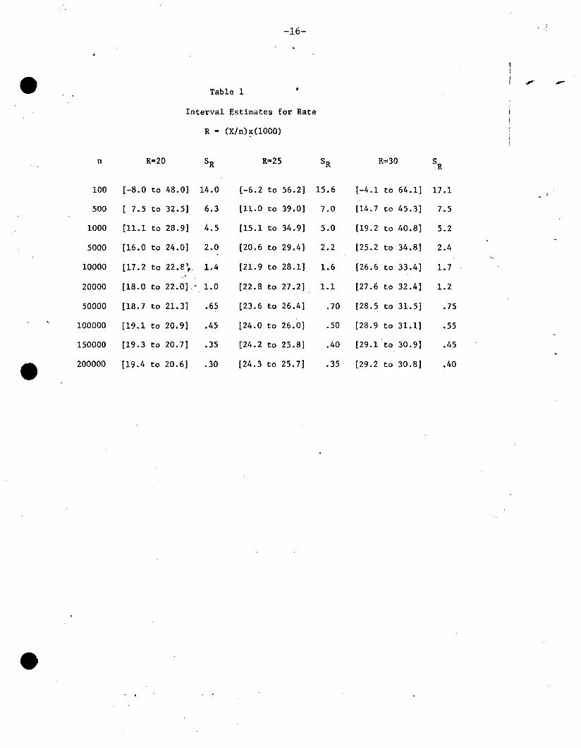
Table 1 illustrates the possible errors of estimation, for various
values of n, and for observed infant mortality rates of R=20,25, and 30.
With R=(X/n)x(1000), the standard error of the estimate is sR = (s)x(lOOO) ,
-4-
where s is the standard error of X/no To allow for the variance of the
observed rate, the interval R+ 2sR may be used as an interval estimate of
the true underlying rate. The table gives lower and upper limits for these
intervals. For small numbers of births (n) the limits are very wide and
little useful information is contained in the data (for n~500 these limits
correspond to approximate 95% confidence limits). Not until the number of
births becomes fairly large, say n~20,OOO can the rates be estimated with
any degree of precision. Conclusions regarding actions to be taken by
health officials must be approached with extreme caution to avoid unnecessary
alarm, wasted time, and expense.
In the following sections, several methods of~atistical analysis
are described and problems of inference are discussed. The examples used
to illustrate these problems refer to infant mortality rates, but the
conclusions apply equally well to perinatal or neonatal rates, and with some
modification, to other vital rates as well. To compare counties within a
state to one another, a method derived from techniques of quality control
is introduced. Next, the problem of finding stable estimates or tests for
small populations is considered. Sequential tests and estimates are
presented, in which data of several years are accumulated to improve the
precision of the estimate. Properties of these procedures are illustrated
and discussed. Methods of Bayesian estimation are explored as a possible
solution where sequential procedures are not sufficient.
Method of Quality Control
Suppose one wishes to determine whether county infant mortality rates
differ from a regional rate or from the state rate by an amount sufficient
to warrant corrective action. A technique which is widely used in industry
has easy application in this context.
-5-
Table 2 gives the infant mortality rates for Michigan counties in
1966. The overall Michigan rate is 22.6 per 1000 (or .0226). Based on this
state rate, the estimated variance of a county mortality rate for a county
with n live births is .0221/n. The variance estimate will be used in
determining whether an observed county rate is significantly larger or
smaller than the state rate. The difference for a particular county is
measured in units of the standard error for that county. The smaller the
number of births, the larger this error will be.
In Table 2, the Z score associated with each county rate is derived
by subtracting the state rate and dividing by the standard error for the
county. (1) Thus, all values are expressed in the same units of measurement.
The extent to which a county rate differs from the state rate depends on the
extent to which Z differs from zero.
According to the Normal distribution, if measurements are expressed
in standard units, and if the measurements arise from the same or similar
populations, then 99% of the time, the measurements should be between
-2.57 and +2.57; 95% of the time they should be between -1.96 and +1.96.
In industrial work, when measurements fall outside of these limits, the
process is considered to be "out of control", and corrective action is
taken. Often, +1.96 are considered "warning limits" and ±2.57 are con-
sidered "action limits". Many variations are possible; for example, action
may be taken only if two consecutive values are "out of control".
(1). In comparing county rates to the state rate, the state rate has beenregarded as a fixed (non-random) value. In fact, the state rateitself is subject to random variation, which calls for somemodification in the variance estimate used. However, if N is thetotal number of live births in the state, the correct varianceestimate is less than the one used here by an amount of p(1-p)/N,which is usually small enough to ignore.
-6-
In studying infant mortality rates, one may only be interested in those
rates that are significantly high. In this case the 99% upper limits are
2.33 and 1.65, respectively, assuming that the Normal distribution is
approximately accurate for these variables. In Table 2, the Z scores can
easily be examined to determine which ones are significantly high. The
rankings of the Z scores differ considerably from the ranking of the
original observed infant mortality rate. In Table 2, a county with 1268
live births has a rate of 30.8 and a Z score of 1.96, outside of the warning
limits, while a county with 177 live births has a rate of 39.5 but a Z
score of only 1.59.
This methodology, while useful in some contexts, points out some of
the problems that arise in small-area estimation. First, as shown, some
counties will not be outside of the control limits, while other counties,
with smaller observed rates (but larger Z scores), will be outside the
control limits. While this is perfectly consistent according to statistical
theory, it may be difficult to explain to a non-statistical administrator.
A second problem arises from the probability of error. As pointed out
above, the rates are random variables, subject to chance variation. The
probability of error in concluding that infant mortality is "out of control"
is limited to .01 or .05 for each county by the structure of the test used,
but with a large number of counties there is a high total probability that
some of the Z scores will be above the control limits when in fact all of
the counties are "in control". In industrial work, this problem is not
serious, since it means only that an occasional batch of items will be
rejected when the overall quality is actually acceptable. But in health
planning, it might mean that a county or other agency embarks on an ex
pensive program unnecessarily.
-7-
When a county has a very large number of live births, the standard
error of estimation of the rate is very small, and differences in infant
mortality rates are easily detected. Thus, in Table 2, a county with more
than 50,000 live births has a Z score of 3.98, by far the largest in the
series, although the observed rate of 25.2 .is well below those of other
counties. In Table 1, it can be seen that with R=25 and n=50,000, the
interval estimate is only 2.8 units long. In such a case, if the observed
rate differs from the state rate by only a small amount, the Z score will be
beyond the control limits. However, since the standard error is so small,
judgements about whether corrective action is needed can be based on
differences in the observed rates themselves.
An alternative approach to the one suggested here is to compare county
rates to a selected "desirable" rate, rather than to a state or regional
rate. One could get considerably different verdicts about which counties
were in or out of control by varying the "desirable" value, but the rankings
of the Z scores would remain the same.
Finally, a major problem in this procedure is the power of the tests
used. The power associated with a particular difference is the probability
of detecting that difference, and is a measure of how well the test detects
the differences it is supposed to detect. It is a function of (a) the level
of the action and warning limits, (b) the size of the difference and (c) the
number of live births. Table 3 gives approximate values of the power of
the suggested test for an action limit of 2.33 and for various sizes of n
and various size differences, denoted as ~ p. The power is based on the
Normal approximation, with variance estimated as .02/n (for higher variance,
the power is reduced). One can see that these procedures are not very
powerful. With a change of 5 deaths per 1000 live births (~ p=.005),
-8-
10,000 live births are needed to detect the change with probability .889.
This means that with n only moderately large, one may conclude that action
is not necessary when in fact it really is needed.
The method of quality control can be useful in assessing observed
rates for small population groups, if the problems discussed above are
taken into consideration. It is more useful to the state or regional
administrator who is evaluating the overall status of a large collection
of small population groups than it is to the administrator associated with
only one of the groups. If his group is a modest size, he knows that there
is considerable chance of error in drawing inferences based on observed
statistics.
Sequential Procedures
According to Table 2, 37 counties in Michigan had observed rates in
1966 which were greater than the overall rate for Michigan of 22.6. However,
only 7 of these 37 counties have Z scores exceeding the warning limit of
1.645, and only 4 exceed the action limit of 2.33. As Table 4 shows, the
power of the test being used to detect differences is quite low when the
number of live births is moderately large, hence we may fail to take
corrective action when it is needed. In this case, a sequential procedure
may be appropriate to monitor the proportion of infant deaths in suceeding
years and to determine when and if the accumulated evidence indicates that
the rate is significantly high.
Frequently health officers wish to compare the infant mortality rate
within a county, beginning in some particular year, to the county's own
rate as averaged over several preceding years. In this case, they may
wish to determine whether the accumulated rate is either higher or lower
than the historical rate, and a two-sided sequential test is appropriate.
-9-
If a new health program has been initiated, a one-sided sequential test
may be used to detect whether there is a decrease.
In the sequential test, the base rate being used for comparison is
expressed as an interval [p',p"]. The test determines at each stage
whether the cumulative observed rate is significantly greater than p"
or significantly less than p' with the interval from p' to p" regarded
as a zone of indifference. A decision can be reached in the minimum
amount of time possible, given the observations generated by the group
being studied. The sequential test also has the advantage of allowing
arbitrary selection of the two error probabilities, probability of in-
correct assumption of increase, and probability of incorrect assumption
of decrease. This overcomes the problem of lack of power due to a
small number of observations, at the cost of a longer waiting period before
a decision is reached. The error probabilities to be tolerated can be
chosen on the basis of practical considerations, according to the
seriousness of the action that would result from either decision.
Let nl
, nZ
' n3
, ..• denote the numbers of live births in successive
years for the group being studied, and let Xl' XZ' X3, ••• be the numbers
of infant deaths.th
The estimated rate up to and including the m year
is the accumulated ratio (XI+X2+"'Xm)/(nl+n2+...+nm) = ~m' A sequence
of intervals [LI,UI ], [LZ'UZ]' [L3,U3], •• is established. As long as the
cumulative estimated rate in a given year is within the appropriate
interval for that year, judgement is reserved until more evidence can be
I d H Of ° h th i I h L h °accumu ate. owever, ~ ~n t e m year, Pm s ess t an m' t e rate ~s
judged to be significantly less than p', or if Pm is greater than Um'
the rate is judged to be significantly greater than p". The intervals
become shorter as the data accumulate, and a difference becomes easier to
-10-
detect.
The threshold values Lm and Um have the form: Lm =(al/Nm)+b and
U =(a2/N )+b, where N is the total number of births up to and includingm m mththe m year. The values aI' a2 , and be depend on the values of p' and p"
chosen for the test, and on the two error probabilities: a, the probability
of incorrectly deciding the rate is greater than p", and S, the probability
of incorrectly deciding the rate is less than p' (2)It is simple to
construct graphs to study this procedure over time. The boundaries of the
decision regions are hyperbolas and appear as in Figure 1. (For very large
values of N , the boundaries converge to the value b, and the interpretationm
of the test changes). In this example, p'=.0200 and p"=.0250; a =.05 and
S = .10. The boundaries of the decision regions are U =(12.66l/N ) +.02247m m
and L =(-9.86l/N) + .02247. Data for two counties in Michigan have beenm m
used to illustrate the procedure, using births and infant mortality for the
years 1960-69. Data for County 1 are plotted with x in the graph.
For this county, while the cumulative observed infant mortality rate re-
mains relatively high, the test does not indicate that action should be taken.
The number of births is so small that even a cumulative ten year rate has a
rather large standard error.
The results in this section show how cumulative data may be used to
reach a decision when the number of births in a single year is not large enough
to yield a statistically significant result. However, in some cases, even the
cumulative number of births may be too small for valid inference.
Moving Average
Even when no test of increase or decrease is involved, cumulative data
methods can be used to improve the accuracy (that is, reduce the standard
error) of an estimate. This is frequently done by using a "moving average"
of a few years data; for example, data from the present and the previous two
years are used to obtain an estimate for the present year. If the true
underlying rate of infant mortality is not changing, this will yield a better
-12-
estimate of the underlying rate.
A moving average is usually obtained by simply averaging the observed
annual rates for the three year period. Thus if Pl ,P2 , and P3 are three
consecutive annual estimates, based on nl ,n2 , and n3
births, the average is
PA = (Pl +P2+P3)/3, which has variance.
1=
9111[p (l-p) ][- + - + -] .nl n2 n
3
If the number of births is small, this estimate can be improved by a very
simple device which reduces the variance of the estimate, thus centering it
more closely on the true value. The improved estimate is obtained by summing
the number of deaths for the three years and dividing by the total number of
variance
2 A
which can be shown to be smaller than sA' (The estimate PB is the same as the
one used in the sequential test).
For example, using the data from County No. 2 in the previous section,
the variance of the three year estimate using data from 1960-61-62 is
.0018547 p(l-p) using PA, and .0018416 p(l-p) using PB. The improvement will
be greatest for counties with very small numbers of births, say less than 100.
The accuracy of the estimate for a given cumulative number of births can be
judged by using Table 1, with n equal to the total number of births.
Bayesian Estimation
For areas of very small population, even the sequential or moving
-13-
average methods suggested in the previous sections may not yield estimates
which are statistically accurate enough for valid inference. An alternative
method of estimation, not commonly used in health statistics, is to assume
some a-priori knowledge about the true underlying rate of infant mortality,
and to make use of this knowledge in a systematic manner. The a-priori
knowledge may be based on some independent information such as a state or
regional rate, or an historical observed rate, and is combined with the data
for the area being studied in order to obtain a more accurate estimate. This,
in effect, combines two independent sources of information, and the procedure
may be varied by the amount of weight placed on the a-priori information.
The amount of weight given to the observed data for the area being studied is
determined by the variance for these data alone, which is again a function of
the number of live births.
The prior information is expressed in the form of a probability
distribution for the true underlying rate p. The most convenient distribution,
for mathematical reasons, is the Beta. Its density function may be expressed
in the form
f (p; m, z)(m+1) != --:---,-:...-:--:-
z! (m-z)!
o otherwise,
z m-zp (l-p) ,O<p<l
where m and z are integers, O<z<m. This distribution has mean (z+1)/(m+2)
and variance [(z+1)(m-z+1)]/[(m+2)2(m+3)]. In this form, the probability
density function may be interpreted as the distribution of p based on a-priori
information that m births results in z infant deaths. (3) Suppose now that
(3)Novick, Melvin R., and Grizzle, James E., "A Bayesian Approach to theAnalysis of Data from Clinical Trials", JASA, Vol. 60, No. 309,March 1965, pp. 81-96.
-14-
observations for the current year give X deaths in n births. The Bayes
estimate p which minimizes the expected squared deviation from the true
underlying value of p is
p = X+z+ln+m+2
This is the mean of a revised or a-posteriori Beta distribution with
parameters z'=z+X and m'=m+n. The revised distribution is a probability
distribution for p based on a combination of a-priori and newly observed
information.
Suppose the estimates in Michigan for 1966 are to be weighted by the
information that the overall state rate is 22.6. This may be expressed,
for example, by using a Beta distribution for p with parameters z=2 and
m=13l (this distribution has mean .02256 and standard deviation .0128).A
The Bayes estimate for each county would be p = (X+3)/(n+133). These
estimates (xlOOO) appear in Table 2 and can be compared to the unweighted
estimates (X/n)x(lOOO). The Baye's estimates have the following properties:
(1) the larger the parameter m is chosen in the Beta distribution, for a
given mean value, the greater the weight placed on the prior information
in the estimate, and (2) for a given Beta distribution, the larger the
number of births in the county, the less the estimate is affected by the
prior information. Thus it can be seen that for counties with large
numbers of births, the two estimates are almost the same, whereas if the
number of births is small, the Bayes estimate is considerably modified in
the direction of the overall state rate.
The Bayes method of estimation may also be used iteratively, with
each year's observed births and infant deaths being used to revise the
previous estimate. After k years of observations, the estimate will be
-15-
Xl + Xz +•....+Xk+z+l
nl + nZ +·····+nk+m+Z
As the number of observed births increases, more and more weight is given
to the observed data as compared to the a-priori information. If the true
underlying value of p is not changing, the estimate will converge to this
value. The procedure cannot be used to detect changes in the pattern of
infant mortality, since new observations are weighted by previous observations
and the a-priori information in making the estimates.
Summary
When statistical indices such as infant mortality rates are computed
for relatively small population groups, the variance of the estimated rate
must be taken into consideration in making inferences about differences
or changes. Statistical techniques such as quality control methods,
sequential procedures, or Bayes estimates may sometimes be helpful in study-
ing these rates. However, for small areas, or small population groups, such
as counties within a state, the variance inherent in these rates may rule
out their use as valid health status indicators.
Acknowledgements:
We thank the Michigan Center for Health Statistics for their assistance.
One of us was supported by Research Career Development Award HD 46344.
-16- ,.'
." -Table 1
Interval Estimates for Rate
R = (X/n)x(1000)
n R=20 SR R=25 SR R=30 SR
100 [-8.0 to 48.0] 14.0 [-6.2 to 56.2] 15.6 [-4.1 to 64.1] 17.1
500 [ 7.5 to 32.5] 6.3 [11.0 to 39.0] 7.0 [14.7 to 45.3] 7.5
1000 [11.1 to 28.9] 4.5 [15.1 to 34.9] 5.0 [19.2 to 40.8] 5.2
5000 [16.0 to 24.0] 2.0 [20.6 to 29.4] 2.2 [25.2 to 34.8] 2.4
10000 [17.2 to 22.8't 1.4 [21.9 to 28.1] 1.6 [26.6 to 33.4] 1.7
20000 [18.0 to 22.0] 1.0 [22.8 to 27.2] 1.1 [27.6 to 32.4] 1.2
50000 [18.7 to 21.3] .65 [23.6 to 26.4] .70 [28.5 to 31.5] .75
100000 [19.1 to 20.9] .45 [24.0 to 26.0] .50 [28.9 to 31.1] .55
150000 [19.3 to 20.7] .35 [24.2 to 25.8] .40 [29.1 to 30.9] .45
200000 [19.4 to 20.6] .30 [24.3 to 25.7] .35 [29.2 to 30.8] .40
-17-
•
Table 2
Michigan Infant Morta1ity-1966
Live Observed Z Z BayesBirths Rate Score Rank Estimate