JOURNAL OF Econometrics ELSEVIER Journal of Econometrics 80 (19971 125-- 165 Statistical inference in the multinomial multiperiod probit model John F. Geweke"-*, Michael P. Keane ~, David E. Runkle t' Department of Economics. Uni~'ersi~' of Minnesota. Minneapolis. MN 55455. USA b Federal Reserve Bank of Minneapolis. Research Department. 250 ~l,larquette Avenue. Minneapolis. Minnesota 35401-0291. USA (Received 1 October 1994; received in revised form July 1996) Abstract Statistical inference in multinomial multiperiod probit models has been hindered in the past by the high dimensional numerical integrations necessary to form the likelihood functions, posterior distributions, or moment conditions in these models. We describe three alternative estimators, implemented using simulation-based approaches to infer- ence, that circumvent the integration problem: posterior means computed using Gibbs sampling and data augmentation (GIBBS), simulated maximum likelihood (SML} es- timation using the GHK probability simulator, and method of simulated moment (MSM) estimation using GHK. We perform a set of Monte-Carlo experiments to compare the sampling distributions of these estimators. Although all three estimators perform reasonably well, some important differences emerge. Our most important finding is that, holding simulation size fixed, the relative and absolute performar-<, of the classical methods, especially SML, gets worse when serial correlation in disturbances is strong. In data sets wtth an AR(I) parameter of 0.50, the RMSEs for SML and MSM based on GHK with 20 draws exceed those of GIBBS by 9% and 0%. respectively. But when the AR(I) parameter is 0.80, the RMSEs for SML and MSM based on 20 draws exceed those of GIBBS by 79% and 37%, respectively, and the number of draws needed to reduce the RMSEs to within I0% of GIBBS are 160 and 80 respectively. Also. the SM L estimates of serial correlation parameters exhibit significant downward bias. Thus, while conventional wisdom suggests that 20 draws of G HK is "enough" to render the bias * Corresponding author. We wish to thank Peter Rossi for useful discussions and Donna Boswell for research assistance, but we are entirely responsible for any errors. Geweke's work was supported in part by National Science Foundation Grant SES-9210070. We thank the f2deral Reserve Bank of Minneapolisfor its support of this research. The views expressed herein are hose of the authors and not necessarily those of the Federal Reserve Bank of Minneapolis or the Vedcral Reserve System. 0304-4076/97/$17.00 ~.:) 1997 Elsevier Science S.A. All rights reserved Pil S0304-4076(97)00005-5
Transcript
JOURNAL OF Econometrics
ELSEVIER Journal of Econometrics 80 (19971 125-- 165
Statistical inference in the multinomial multiperiod probit model
John F. Geweke"-*, Michael P. Keane ~, David E. Runk le t'
Department o f Economics. Uni~'ersi~' o f Minnesota. Minneapolis. MN 55455. USA b Federal Reserve Bank o f Minneapolis. Research Department. 250 ~l,larquette Avenue. Minneapolis.
Minnesota 35401-0291. USA
(Received 1 October 1994; received in revised form July 1996)
Abstract
Statistical inference in multinomial multiperiod probit models has been hindered in the past by the high dimensional numerical integrations necessary to form the likelihood functions, posterior distributions, or moment conditions in these models. We describe three alternative estimators, implemented using simulation-based approaches to infer- ence, that circumvent the integration problem: posterior means computed using Gibbs sampling and data augmentation (GIBBS), simulated maximum likelihood (SML} es- timation using the G H K probability simulator, and method of simulated moment (MSM) estimation using GHK. We perform a set of Monte-Carlo experiments to compare the sampling distributions of these estimators. Although all three estimators perform reasonably well, some important differences emerge. Our most important finding is that, holding simulation size fixed, the relative and absolute performar-<, of the classical methods, especially SML, gets worse when serial correlation in disturbances is strong. In data sets wtth an AR(I) parameter of 0.50, the RMSEs for SML and MSM based on G H K with 20 draws exceed those of GIBBS by 9% and 0%. respectively. But when the AR(I) parameter is 0.80, the RMSEs for SML and MSM based on 20 draws exceed those of GIBBS by 79% and 37%, respectively, and the number of draws needed to reduce the RMSEs to within I0% of GIBBS are 160 and 80 respectively. Also. the SM L estimates of serial correlation parameters exhibit significant downward bias. Thus, while conventional wisdom suggests that 20 draws of G HK is "enough" to render the bias
* Corresponding author.
We wish to thank Peter Rossi for useful discussions and Donna Boswell for research assistance, but we are entirely responsible for any errors. Geweke's work was supported in part by National Science Foundation Grant SES-9210070. We thank the f2deral Reserve Bank of Minneapolis for its support of this research. The views expressed herein are hose of the authors and not necessarily those of the Federal Reserve Bank of Minneapolis or the Vedcral Reserve System.
0304-4076/97/$17.00 ~.:) 1997 Elsevier Science S.A. All rights reserved Pi l S 0 3 0 4 - 4 0 7 6 ( 9 7 ) 0 0 0 0 5 - 5
126 J.F. Geweke et aL / Journal o f Econometrics 80 (1997) 125-165
and noise induced by simulation negligible, our results suggest that much larger simula- tion sizes are needed when serial correlation in disturbances is strong. (.t~, 1997 Elsevier Science S.A.
Kevn'ords: Bayesian inference; Discrete choice; Gibbs sampling; Method of simulated moments; Simulated maximum likelihood; Panel data JEL clasMfication: C35; C15
1. Introduction
Discrete economic choices are often made repeatedly over several time peri- ods. Examples include the. choice of which brand of a frequently purchased product category to buy on each successive ourchase occasion and which of several industries or occupations to work in during each year of one's life. A multinomial multiperiod probit (MMP) model can be a reasonable frame- work for studying choice behavior in such situations. However, the very high dimensional integrations necessary to form the likelihood function, posterior distribution, or momer, t conditions for inference in the M M P model have until recently precluded its application. Rapid advances in simulation-based ap- proaches to inference (McFadden, 1989; Pakes and Pollard, 1989; Keane, 1994a; McCulloch and Rossi, 1994) have now made both classical and Bayesian mference feasible. These advances have led to several interesting applications of the MMP model. These include sequential models of the decision to work (Keane, 1994a), brand choice (Elrod and Keane, 1995, Keane, 1994b, McCulloch and Rossi, 1994), choice of residential location (Hajivassiliou et al., 1996), and the probability a country will default on loans (Hajivassiliou and McFadden, 1994L
Despite this burgeoning list of applications, there has been no systematic comparison of the sampling distributions of alternative estimators in the MMP model in samples representative of these applications. The goal of the present paper is to provide such a comparison. First, we describe estimators based on three alternative approaches to inference: simulated maximum likelihood (SML) estimation using the Geweke-Hajivassiliou-Keane (GH K) recursive probability simulator, method of simulated moment IMSM) estimation using the GHK simulator, and posterior means computed using Gibbs sampling and data augmentation (GIBBS). We perform a set of Monte-Carlo experiments to compare the sampling distributions of the respective estimators. The experi- mental design allows the impact of three important features of the data on the performance of the methods to be assessed: (1 ~ serial correlation of the random components of utility, (2) serial correlation of the exogenous variables, and (3) contemporaneous cross-alternative correlations of the random components of utility.
J.F. Geweke et al. / Journal ~ f Econometrics 80 (1997) 12J-165 127
Besides features of the data, it is also important to consider how simulation size affects results. In the first set of experiments we hold the number of draws used to implement the GHK probability simulator fixed at 20. We choose 20 because conventional wisdom suggests this number is sufficient to render the bias intrinsic to the SML estimator negligible. For instance, Brrseh-Supan and Hajivassiliou (1993) conclude that 'In our Monte Carlo experiment, 20 replica- tions were sufficient to produce a negligible bias', z,n.~ this conclusion has been influential. In fact, existing applications of SML generally use 20 or fewer draws. In a second set of experiments, we examine how performance of the classical estimators is affected by the number of draws used to implement the G H K probability simulator. In both experiments we set the number of cycles of the Gibbs sampler at 5000, since we find that this is sufficient to render the simulation noise in the posterior means very small as a fraction of root mean square error (RMSE).
Although all three estimators perform reasonably well in our experiments, some important differences emerge. Our most important finding is that, holding simulation size fixed, the relative and absolute performance of the classical methods, especially SML, gets worse when serial correlation in disturbances is strong. Consider the RMSEs of the SML and MSM point estimates and GIBBS posterior means around the data generating parameter values. In data sets with an AR(I) parameter of 0.50, the RMSEs for SML and MSM based on G H K with 20 draws exceed those of GIBBS by 9% and 0%, respectively. But when the AR(I) parameter is 0.80, the RMSEs for SML and MSM based on 20 draws exceed those of GIBBS by 79% and 37%, respectively, and the number of draws needed to reduce the RMSEs to within 100,~ of GIBBS are 160 and 80 respec- tively. Furthermore, the SML estimates of serial correlation parameters exhibit significant downward bias and this becomes insignificant only when 160 to 320 draws are used. Thus, contrary to conventional wisdom, 20 draws is not nearly 'enough" when serial correlation is strong.
This is the first systematic study of the performance of simulation-based approaches to inference in the M M P model in representative samples. There are five precursors of this work that are worth noting. Brrsch-Supan and Hajivas- siliou (1993) considered the distribution of the SM L estimates of a single slope parameter in a cross-section trinomial probit model (with all other parameters held fixed at true values) using a single artificial data set, but varying the draws used in constructing the G H K simulator. McCulloch and Rossi (I 994) provide Gibbs sampling data augmentation algorithms for the cross-section and panel probit models with random coefficients, but they do not allow for serial correla- tion in disturbances or compare sampling distributions ofalternative estimators, Geweke et at. (1994) compared the sampling distributions of the SML, MSM and GIBBS estimators in the single-period multinomial probit model. Keane (1994a) studied the sampling distributions of the MSM and SML estimators based on the GHK probability simulator in the multiperiod probit model.
t 2 8 d.F. Geweke et al. /dourna l o f Econometrics 80 (1997) 125-165
However, he only considered binomial probit models, did not consider Bayesian methods, and did not evaluate the influence of simulation size on the perfor- mance of the alternative methods. Hajivassiliou and McFadden (1994) s tudy sampling distributions of S M L and simulated score estimators in the multi- period binomial probit model.
in Section 2 we describe the M M P model. Section 3 describes the SML and MSM estimators. In Section 4 we describe the GIBBS estimator. Section 5 lays out the design of our Monte-Car lo study, Section 6 presents results, and Section 7 concludes.
2. The model
Assume that agents choose among a set of J mutually exclusive alternatives in each of T time periods. If individual i chooses alternative j at time t, he/she derives utility
U o , = X ; j , flj+~:i# ( J = 1 . . . . . J ; t = 1 . . . . . T),
where X 0, is a p × 1 vector of exogenous variables, /~j is a p x l vector of corresponding coefficients, and e.~jt is a r andom shock to utility that is known to the agent but not to the econometrician. Cho ice j is made at t ime t if Uor > U m for all k ~ j . The econometr ic ian observes the choice
d~j t=.~l i f i chooses j a t time t otherwise,
but not the utility of any choice. The M M P model is obtained by assuming
g i ~ (g..i! 1 , " ' " , g ' i J l , " ' " , g i l T , "" ,~ i . t r ) ' "~" IIDN(0,E), E = [-o'i~ ].
Since choices only depend on utility differences, it is conventional to measure utility relatice to alternative J. Since the scale of utilities is indeterminate, it is also conventional to normalize by setting the variance of the error term correspond- ing to the first alternative in the transformed model equal to one. Thus, we define
U*, = (U O, -- U/a,)(tr t t + aj~ -- 2tr t j ) - 1/2
= [ ( X ; j , t l j - X ; j , # ~ ) + (~:/j, - ~ :u , ) ] (61 , + 0"11 - - 20"t j ) - ,/2
= x * ; f l ~ + ~* , ( j = 1 . . . . . a ; t = 1 . . . . . r ) , (2.1)
where X~t ( j -- 1 . . . . . J ) is the appropr ia te t ransformation o f X i j t ( j = 1 . . . . , J ) and f l ' ~ ( j= 1 . . . . . J ) is the appropria te t ransformation of f l j ( j = i . . . . . J). (Notice that U~5, = 0 and ~5, = 0.) We further define
£ ~ = ( 8 i l , . . . . . . L J - I . t . . . . . & / I T . . . . . P ' i . J - , . T)'
~.~ ,.0 IIDN(O,'~*), E* --- loCI , (2.2)
J.F. Geweke et al. / Journal o f Econometrics 80 (1997) 125-165 129
where Y-* is the correspo-,,ding appropr ia te t ransformation of X; by construc- tion, al ' l = I.
In the notat ion of the transformed model, choice j is made at time t if
Ui*, > Ui*, for all k ¢-j (j = 1 . . . . . J). (2.3)
in order to have a compact nota t ion for the sequence of choices observed for person i, define
d a = ( d i l , . . . . , d i j , ) , dt = (d~t . . . . . di,), and j , = { j ld i j , = 1}. (2.4)
If P(d~) denotes the probabil i ty that i chooses the sequence dl,
P(d f ) = P(U~j, . , > Ui*, V k ~ Ji,, t -- ! , . . . , T )
v * , a * _ X * , t~*Vk ¢ j i , , ( t = 1, T) ' ] . = P [~,.*i,., - e l , > - ~ , , , v k , j , . , , - j , - - . ,
If the ~ , are serially independent, then this is the product of T integrals each of dimension J -- I. However, if the e*~ are serially correlated, this is in general a T ( J - l) variate integral. As T and /o r J grow, inference requiring exact evaluation of such integrals rapidly becomes infeasible. Much o.f the earlier work on the M M P model sought to avoid this problem by imposing low-order factor structures on ~*. Fo r example, if a r andom effects structure is imposed, the order of integration is reduced to 2 ( J - - 1). The goal of simulation~based inference is to allow a richer covariance structure to be used.
In this paper we consider a special case of the model (2.1)-(2.4) in which the ~.r*~ are s tat ionary first-order autoregressive EAR(I)] processes and in which the X*t are divided into two sets of covariates: a set -~*-t that is constant across alternatives (which can be thought of as containing characteristics of agent i) and a set Zi*t that varies across alternatives (which can be thought of as containing attributes of alternatives, such as price or quality), but for which the corresponding coefficients are restricted to be equal across alternatives.
These decisions are motivated by a desire to s tudy models that are practical. Note that even if the high-order integration problem can be solved by simula- tion techniques, unless J and T are both quite small it is not feasible to estimate an unrestricted ~ * matrix which would contain T 2 ( J - 1)2/2 free parameters. This motivates our decision to study models in which the errors follow a station- ary AR(1) process. Our parti t ioning of the covariates into two types is motivated not only by a desire to imitate applications, but also by the fact that likelihood surfaces in the muitinomial probit model tend to be very flat unless one includes covariates that vary across alternatives (see Keane, 1990).
We next set out notat ion for the specific M M P model used in our experi- ments. Part i t ion each coefficient vector fl~' -- (~[~", 7') reflecting cross-equation constraints of the form employed in the experiments, and conformably part i t ion
130 J,F. Geweke et at. /Journal o f Econometrics 80 (1997) 125 165
= (Xo, , Z u,). F u r t h e r define the mat r ices
[i o o [io o 2 , 2*, ' , . . . o p ~ - . - o
o - .
0 .-- X;% 0 "'" pt.
[ z?,;
z* = ] Z?~, LZ~L
where L = d -- 1 a n d Ipjl < I [j = 1 . . . . ,L) . C o n f o r m a b l y def ine
~ : , * = " , u ~ , = " , g * = : , p = .
In ma t r i x no ta t ion , the m o d e l is then
u,*, 2"17" + z~.~ + * ~ - F, i t •
T h e d i s t u rbances ~:* fol low s t a t i o n a r y AR( I ) processes:
Thus , the vi, a re serially uncor re l a t ed but co r re la ted ac ros s a l ternat ives . Wi th this s t ruc ture , a ~ = ,/,jk/(l - PkP.i ]. T h e a s s u m p t i o n tha t R is d i agona l is specific to the n o r m a l i z a t i o n on cho ice d in (2. I). In general , if R is d i agona l for the given no rma l i za t i on , it will no t be d i agona l for a l t e rna t ive no rma l i za t ions . T h e d iag- ona l i ty a s s u m p t i o n m a d e here will be m o s t a p p e a l i n g when choice J is a base l ine decision, such as a no pu rchase op t ion in a b r a n d choice m o d e l o r a no w o r k : ,p t ion in an o c c u p a t i o n a l cho ice model , for which it is r e a sonab l e to a s s u m e util i ty is n o n r a n d o m .
3. Classical approaches to inference
3. !. Simulation o f choice sequence probabilities
Classical e s t i m a t o r s for the M M P m o d e l rely on M o n t e - C a r l o s imula t ion o f the choice sequence p robab i l i t i e s P(dl) a n d subs t i tu t ion of these s imula ted probabi l i t i e s in to l ike l ihood funct ions or m o m e n t condi t ions . In an extensive
J.F. Geweke et al. / Journal o f Econometrics 80 (1997) 125-165 i 31
study of alternative methods for simulation of multinomial orthant probabiht- ies, |lajivassiliou et al. (1992)conclude that the G H K probability simulator, due to Keane (1990), Geweke (1991), and Hajivassiliou and McFadden (! 994L is the most accurate of all methods considered. Geweke et al. (1994), in a Monte-Carlo study of alternative simulation estimators in the single-period multinomial probit model, concluded that classical methods based on GHK substantially outperformed classical methods based on kernel smoothed probability simula- tors. For these reasons, we rely exclusively on G H K to simulate choice probabil- ities when implementing classical estimators in this paper. In Appendix A we describe how to apply the GHK algorithm to simulation of choice sequence probabilities in the MMP model of Section 2. Below, we let P6HK(dil/~*, X*, X*) denote the GHK simulator of the probability of ~.[,oice sequence d~.
3.2. Classical estimation methods
The two classical estimation methods we consider are simulated maximum likelihood (SML) and method of simulated moments {MSM). The SML es- timator maximizes the simulated log-likelihood function, which is obtained simply by substituting GHK simulators of choice sequence probabilities into the log-likelihood function:
N
L([~*, E*) = ~ log P~nK(d;l/~*, X*, X*). i = t
The SML estimator is consistent if M / ( N ) jlx -* oc as N --* o'z. (For proofs, see Lee, 1992, 1995; and Gourieroux and Monfort, I993.)
Direct application of McFadden's (! 989) MSM estimator to the i M P model would involve indexing all possible choice sequences s = 1 . . . . . j r and defining choice indicators d~ = 1 if i chooses sequence s and 0 otherwise. Then form the MSM estimator by solving the moment conditions:
N j r
E W,.[d,s - P ,,K X sM, = 0. / = 1 s = l
This MSM estimator is consistent for fixed M. This direct approach is not feasible because of the computational burden involved in simulating probabilit- ies of J r sequences and forming j r weights.
Keane (I 990) proposed the eomputationally feasible alternative of factoring the sequence probabilities into transition probabilities and forming the alterna- tive estimator:
N T d
Y w j, P .Kld, ,l,t, . . . . . = 0 , i = l I = i j = l
132 J.F. Geweke e! aL / Joto'nal o f Econometrics 80 (1997) 123-165
where the transition probabilities are simulated using ratios of GHK-simulated choice probabilities,
PGaK (do, I di l . . . . . di., - 1) - /~C.HK(dil . . . . . d i . , - t , dij,)
PGH~(d. . . . . . d,.,_ , )
Although this gives a biased simulator of the transition probability, an MSM estimator of this form is consistent if M / ( N ) t/2 ~ ~ as N ~ ~ (see Keane, 1994a). In addition, Keane (1994a) finds in a Monte-Carlo study that it has small sample properties superior to SML for the multiperiod binomial probit model, especially when serial correlation is strong.
4. Bayesian inference using the Gibbs sampler
Bayesian inference using the Gibbs sampler (Gelfand and Smith, 1990) and data augmentation (Tanner and Wong, 1987) has been applied to the M M P model by McCulloch and Rossi (1994). Our approach is similar, but differs in four respects: Here, all priors are proper whereas MeCulloeh and Rossi use improper priors fer fl*; we include autoregressive error components; stationar- ity is enforced through data augmentation of presample random utilities, rather than through explicit restrictions on E* (see step 2 below); and the coefficients of covariates are fixed ~ather than random.
To provide a description of the Gibbs algorithm in generic notation, let 17, 0 and Y denote vectors of latent utilities, model parameters, and observed choice data, respectively. Let p (0, ~1 Y ) denote the joint posterior density function for 0 and 17 conditional on Y. Suppose there is a partition of the parameter vector 0 into B subveetors, 0' =(0~1~ . . . . . 0~B~), such that the conditional posterior densities p(Oo~ I Oij ~, j ~ i, 17, Y ) and p( F I 0, Y) are of sufficiently simple form that it is practical to draw random subvectors tT,~ and 17 from these conditional densities. The Gibbs algorithm starts with an initial value (0 Ira, ~,lm) in the support of p(O, ~ I Y ) , and then draws in turn each of the subveetors ]?, Ott ~ . . . . . 0~m from the appropriate conditional density. After each draw, the corresponding initial value subveetor is replaced by the new subveetor, until after a complete iteration an updated vector (0 ~ t ~ 17 ~ t ~) is obtained. After the ruth iteration we obtain the draw (0 Imp, 17t=~). As m grows larger the sample of (0, 17) draws converges in distribution to the joint posterior distribution. Posterior means for the elements 0 are then approximated using arithmetic averages ef the corresponding draws.
To describe the implementation of the Gibbs algorithm in the M M P model, some minor changes and extension in notation are necessary. Let the U*, , X ~ , , .,jP*, and e.-*..,~, continue to denote the latent utilities, covariates, coeffi- cients, and disturbances of the transformed model, respectively, except that the
J.F. Geweke el al, / Jonrnal o f Econometrics 80 (1997] 125-165 133
transformatios~ (2.1)is replaced by
U L = ( U u , - Uij~)
--u,~'~ "u, ( j = l , J ; t = I , T ) .
The values of the fl* change accordingly, as does ~' = var(e* - Re* ,_ i ). The matrix R is unaffected.
Since the restriction aT, = 1 has not been imposed, the parameters at this point are unidentified. In order to achieve identification, the following proper prior distributions were employed throughout the experiments:
/~* --~ N(0,1r); ~, --~ N(0, IT); pj "-- TN(0.5,0.25); , p - t ... W 0 0 / L , 10).
The proper prior distribution for ~ centers the ~jj, which otherwise would be identified only up to a scale factor, about 1.0. This in turn induces a proper posterior distribution for the/~* and 7, even if the priors for these coefficients were flat and improper. (This technique was introduced by McCuUoch and Rossi (I 994).) The posterior distribution of these parameters induces a posterior distribution on g * = vat(e*), with aj* = ~jt,/(1 -p jp~) . Using the normaliz- ation set forth in Section 2, parameters of interest are ~ ' (oi '])- t/z (j = 1 . . . . . L); "/(~Tt )- l/z; p~ fo r j = 1 . . . . . L; and the elements of the upper triangular matrix A*, where A* 'A* = (a*~)-t ,p. To make drawings from the posterior distribu- tions of these functions it is necessary only to transform the drawings of the ~*, ~, p j . and ~'. in the experiments we will see that posterior s tandard deviations are very ~mall relative to the priors, and on this basis it is reasonable to conjecture that results would be quite similar for other diffuse but proper priors.
We employ a six-block Gibbs sampling da ta augmentat ion algorithm in which the blocks are: (1) ~he latent utilities U ' t ; (2) the presample values of the errors, e~0; (3) the p j; (4) '~be matrix ~; (5) the vector fl* = (]I*', . . . . /~/~')'; and (6) the 7. Although McCulloch and Rossi (1994) descr,.'be the structure of a Gibbs sampling data augmentat ion algorithm for a M M P model with random effects, the complications introduced by our addition of autoregressive error compo- nents are sufficiently great (including the addition of the new blocks 2 and 3 and changes necessary in other blocks) that we provide a detailed description of the algorithm for the present model in Appendix B.
In our experiments, the first 200 Gibbs iterations were discarded to allow "burn in' from the initial drawing from the prior distribution. Inspection of these iterations showed that parameter values moved from well outside the concentra- tion of the posterior distribution to its concentration in fewer than 100 iter- ations. Arithmetic averages of the parameters of interest over the next m = 5000 iterations were used to approximate posterior means. The standard errors of these Monte-Carlo approximations were asse.~.,.ed as described in G~.weke
134 J.F. Geweke et aL / donrnat o f Econometrics 80 (1997) 125-165
(1992). Typical ly, this s t anda rd e r ro r was less than 10% o f the pos te r ior s t a n d a r d devia t ion for the exper iments under taken .
T h e a p p r o x i m a t e pos te r io r means ob ta ined via the G i b b s sampl ing da t a a u g m e n t a t i o n a lgo r i thm cons t i tu te the G I B B S es t imators that we c o m p a r e with the S M L and M S M est imators . Pos te r io r means , given the priors assumed, cons t i tu te well-defined es t imators with sampl ing- theore t ic propert ies. Thus, ou t a p p r o a c h here is del iberately frequentist. A truly subjective Bayesian wou ld have no reason to enter ta in e i ther the M S M or S M L methods , and wou ld have little interest in pos ter ior means given pr iors o f convenience.
5. Experimental design
In o u r M o n t e - C a r l o experiments , we cons ider a three a l ternat ive model (d = 3~ with T = 10. We cons t ruc t 20 artificial da t a sets o f size N = 500 using the da t a genera t ing process:
u*l , -- 0.5 + 1 x * + I Z * , + ~:~,
u & , -- - 1.2 + i x ? , + 1z?,2 + ,:*,
and of course, U*3r = 0.0 by o u r normal iza t ion . The r a n d o m shocks to utility evolve acco rd ing to
~:*n = p l s * l . , - i + v , ,
~:,'*z, = p,_~:*,..,- t + vi2,
,',,,l--[' o ]r,,,,,l vi2,_l a]~- " w/l--(a]~2} 2 Lq;2, J
with tl~r ~ I IDN(0 , 1(I - p 2 } ) . In all the genera ted data , Pt = P., = P. In the no ta t ion o f Sect ion 2,
lq ' = ( 0 5 , 1, i)' , / ;* = ( - 1.2, 1, i)'
x~*i,, = x * , , , - x ~ , x,*,,,_ = z * , , , x~ , ,_ =_ z*2,
[~% = 1 ~ - 7,
where X~u refers to the lth e lement of the X.*. vector. The regressors are ~dg cons t ruc t ed as follows:
In our first experiment, we set the number of draws used to form the G H K simulator at 20, and consider 12 different data structures given by the 3 x 2 × 2 full factorial design,
p, = P2 -- 0.50 or 0.80; a~'2 = 0.50 or 0.80; ~b-" = 0 or 0.50 or 0.80.
These correspond to 'low" and "high" serial correlat ion and cross correlat ion in the random elements of utility and "no', 'low', and "high" serial correlat ion in the exogenous variables, respectively, in the second experiment we vary the number of draws used to implement G H K , using two of the these data structures (chosen as described in Section 6.2).
6. Results
6.1. Experiment I - - effect o f data structure on petformance o f the estimators
The results of the Monte-Car lo experiments based on the 12 different data structures are reported in Tables 1-12. Fo r GIBBS we report: (1) the mean of the posterior means across the 20 replications, ~; (2) the RMSE of the posterior means a round the data generating values; and (3) the mean of the posterior s tandard deviation across the 20 replications, PSD. F o r S M L and MS M we report three statistics for each parameter in each model: (!) the mean of the point estimates across the 20 replications, 0; (2) the root mean square er ror (R MSE) of the point estimates a round the data generating values; and (3) the mean of the
asymptotic s tandard errors across the 20 replications, ASE. In the remainder of this section, we compare the performance of the different estimators in each experiment, focussing on RMSE as the criterion of performance. We also
examine the ASE and PSD, because, for purposes of inference, it is desirable that ASE or PSD be similar to RMSE.
In Table 1 we consider 20 artificial da ta sets generated from the data structure in which Pi = P2 = 0.50, a]'2 ---- 0,50, and q)2 = 0. This is the case of low serial and cross correlat ions of the disturbances combined with no serial correlat ion in the covariates. For GIBBS and MSM, the ~ are close to the data generating values for all 9 model parameters. SML, on the other hand, while producing estimates close to the data generating values for most model parameters, exhibits severe bias in estimatipg the AR(I) parameters. In particular, the mean SM L point estimate of p2 is 0.376, while the data generating value is 0.500. If we use the empirical RMSEs divided by (20) t/z to form t-tests for the estimated
Tab
le 1
C
orr0
1,,
ah,)
= 0.
5, P
t =
tta2
=
0.5.
Cor
r(x,
, x,_
1) =
0.0
Bay
esia
n in
fere
nce
MS
M-G
HK
S
ML
-GH
K
0
DG
P
~
RM
SE
PSD
(~
R
MSE
ASE
~7
RM
SE
A'-S'E
EaT:
0.
500
0.47
0 0.
085
0.08
0 0.
520
0.08
6 0.
088
0.56
6 0.
110
0.07
5 a*
2 0.
866
0.88
4 0.
053
0.06
5 0.
880
0.05
6 0.
070
0.93
3 0.
084
0.05
9 #;
0.
500
0.49
6 0.
023
0.03
2 0.
504
0.02
4 0.
031
0.45
5 0.
050
0.02
8 ,o
* 0.
500
0.47
5 0.
040
0.06
1 0.
480
0.04
8 0.
065
0.37
6 0.
131
0.05
1 /t*
1 0.
500
0.49
2 0.
025
0.03
6 0.
499
0.02
5 0.
032
0.50
2 0.
024
0.03
0 [~
*a
- 1.
200
- 1.
210
0.06
5 0.
083
- 1.
204
0.07
4 0.
078
- 1.
231
0.07
9 0.
077
/t~' 2
1.00
0 0.
988
0.02
4 0.
037
0.99
5 O
.021
0.
032
0.99
3 0.
022
0.03
2 [~*
,_z
1.00
0 0.
974
0.05
9 0.
058
1.00
5 0.
056
0.05
4 1.
012
0.05
7 0.
05I
-.*
1.00
0 0.
995
0.02
4 0.
037
0.99
3 0.
028
0.03
3 0.
995
0.02
5 0.
032
t Tab
le 2
C
orr0
h,,
)?2,
) = 0
.5,
th =
92
= O
.5, C
orr(
x,..'
q _ 1
) = 0
.5
e,,
Bay
esia
n in
fere
nce
MS
M-G
HK
S
ML
-GH
K
(; D
GP
~ R
MSE
PS
D
V
RM
SE
ASE
I~
R
MSE
A
SE
oe,
a:~,
0.
500
0.45
7 0.
069
0.09
2 0.
505
0.08
8 0.
124
0.59
7 0.
131
0.08
8 a*
: 0.
866
0.87
2 0.
070
0.07
7 0.
854
0.09
3 0.
081
0.92
2 0.
096
0.06
8 p]
' 0.
500
0.50
6 0.
022
0.02
5 0.
509
0 32
5 0.
026
0.47
6 0.
034
0.02
3 p~
0.
500
0,48
9 0.
037
0.05
0 0.
496
0.03
6 0.
057
0.41
6 0.
091
0.04
3 fl~
'l 0.
500
0.49
3 0.
018
0.03
2 0.
499
0.01
8 0.
O31
0.
502
0.01
7 0.
028
fl~t
-
1.20
0 -
1.20
8 0.
090
0.11
1 -
1.18
0 0.
115
0.10
6 -
1.23
5 0,
104
0.10
2 f.~
L,
1.00
0 0.
989
0.02
9 0.
042
0.99
5 0.
029
0.04
0 0.
997
0.02
9 0.
038
[1"_,2
!.0
00
0.94
7 0.
091
0.08
0 0.
974
0.10
4 0.
084
1.01
6 0.
087
0.07
2 -,*
1.
000
0.98
7 0.
034
0.04
3 0.
981
0.03
8 0.
040
0.98
7 0.
034
0.03
9
I
Not
e: 0
~ p
aram
eter
. D
GP
--
data
gen
erat
ing
valu
e, ~
- av
erag
e pa
ram
eter
est
imat
e, R
MS
E -
= ro
ot m
ean
squa
re e
rror
, P
SD
-
aver
age
post
erio
r
stan
dard
dev
iati
on,
ASE
~ a
vera
ge a
sym
ptot
ic s
tand
ard
erro
r.
Tab
le 3
C
orrl
lht,
l#:,}
= 0
.5, P
l= P
- =
0.5,
Cor
r(x,
. x,-
,) =
0.8
Bay
esia
n in
fere
nce
0 D
GP
~
RM
SE
PS
D
a~2
0.50
0 0.
438
0.t1
3 a*
_,
0.86
6 0.
860
0.07
I pT
0.
500
0,50
7 0.
025
p~
0.50
0 0.
494
0.05
4 /JT
~ 0.
500
0.48
8 0.
027
fl_~t
-
1.20
0 -
1.19
3 0.
111
//*z
1.12
00
0.97
4 0.
041
lIT,
1.00
0 0.
939
0.09
3 -,*
1,
000
0.98
6 O
.041
i T
able
4
MS
M-G
itK
;'~M
SE
ASE
SM
L-G
HK
RM
SE
ASE
0.0%
0.
535
0.13
7 O
. 137
0.
574
0.07
9 0.
861
0.O
97
0.08
5 0.
931
0.02
5 0.
507
0.02
9 0.
026
0.48
3 0.
045
0.49
0 0.
064
0.05
2 0.
429
0,03
4 0.
498
0.02
9 0.
034
0.50
3 0.
115
- t.1
86
O. 1
24
0.11
2 -
1.24
3 0.
046
0987
0.
038
0.04
4 0.
991
0.07
7 0.
982
O. 1
00
0.08
8 1.
006
0.04
7 0.
986
0.03
9 0.
044
0.99
6
0.12
2 0.
085
.'n
0.10
1 0.
070
0.03
2 0.
024
.~
0.08
6 0.
040
0.02
7 0.
031
p,.
0.11
5 0.
104
0,03
3 0.
041
7 0.
065
0.07
0 0.
036
0.04
2
, g.
RM
SE
AS-E
~,~
0.13
8 0.
067
0.16
1 0.
064
i
0.04
8 0.
014
0.12
4 0.
027
0.03
0 0.
033
0.06
2 0,070
0.02
3 0.
030
0.05
7 0.
046
0.02
5 0.
030
.~
Cor
rOh,
, ~1-
,,) =
O.5
, Ih
= P.
' = 0
.8,
Cor
r(x,
x~-
O =
0.0
Bay
esia
n in
fere
nce
0 D
GP
I~
R
MSE
P
SD
MS
M-G
HK
RMSE
AS
I~
SM
L.G
HK
a*_,
0.
500
0.50
6 0.
053
a[2
0.86
6 0.
927
0.08
9 Pt
' 0.
800
0.79
5 0,
013
p~
0.80
0 0.
771
0,03
9 [IT
~ 0.
500
0,49
6 0.
025
[l_~l
-
1.20
0 -
1.20
5 0.
066
Jt?z
1.oo
o 0.
985
0.02
6 j/*
,, 1.
000
0.97
2 0.
060
• ,*
t.000
0.
991
0.03
0 I
0,07
9 0,
567
0.12
1 0.
107
0.62
0 0.
084
0.89
2 0,
109
0.09
7 1.
012
0,02
7 0.
808
0.02
2 0.
018
0.75
5 0.
047
0,79
0 0.
042
0.03
7 0.
680
0.04
1 0.
500
0.03
3 0,
042
0.49
9 0.
085
- 1.
176
0.09
0 0.
084
- 1,
218
0,03
8 0.
985
0.02
8 0.
037
0.99
0 0.
056
0.98
9 0.
O61
0.
056
1.00
3 0.
039
0.98
2 0.
038
0.03
6 0.
991
Tab
le 5
Co
rrOh
,,q,_
,) =
0.5,
pt
= ~J
z = 0
.8.
Cor
rlv,
, x,-
,) =
0.5
=o
Bay
esia
n in
fere
nce
0 D
GP
~
RM
SE
P
SD
aT:
0.50
0 0.
455
0.08
4 a*
, 0.
866
0.88
8 0.
072
p*
0.80
0 0.
798
0.01
6 p_
*, 0.
800
0.78
3 0.
026
/t1'l
0.50
0 0.
497
0.01
8 [l*
~ -
1.20
0 -
1.19
1 0.
096
fl'(2
t.000
O
.991
0.
028
1,~*:
1.
000
0.93
2 O
. I 01
".
* 1.
000
0.98
0 0.
040
¢ Tab
le 6
MS
M-G
HK
RM
SE
A
SE
SM
L-G
HK
RM
SE
A
SE
0.08
8 0.
529
0.13
2 O
. 155
0.
606
0.08
0 0.
830
0.09
6 0.
108
1.00
t 0.
020
0.80
5 0.
020
0.01
6 0.
768
0.03
5 0.
791
0.03
9 0.
038
0.70
2 0.
041
0.50
1 0.
029
0.04
1 0.
501
0.11
1 -
1.12
1 0.
140
0.11
6 -
1.23
3 0.
044
0,99
5 0,
037
0.04
3 1.
000
0.07
5 0.
960
0.09
1 0.
090
0.99
6 0.
045
0.96
6 0.
054
0.04
4 0.
987
0.14
0 0.
076
0.15
7 0.
073
0.03
6 0.
013
0.10
4 0.
025
0.03
0 0.
033
0.11
0 0.
097
0.03
1 0.
038
0.O
82
0.06
6 0.
038
0.03
7
Cor
r0h,
, q_
,,) =
O.5
, th
= P_
, = 0
.8,
Cor
r(x,
..~;,-
~1 =
0.8
Bay
esia
n in
fere
nce
0 D
GP
0
RM
SE
aT_,
0.50
0 0.
4 i 8
0.
139
0*2
0.86
6 0.
870
0.06
4 I~
' 0.
800
0.79
5 0.
0t 5
p_
*, 0.
800
0.78
1 0.
029
p,*~
0.
500
0.48
5 0.
025
[3*,_t
- 1.
200
- 1.
189
0.12
5 P~
2 I.O
00
0.95
9 0.
063
[l~z
1.00
0 0.
920
0.10
9 • ,*
1.
000
0.97
3 0.
059
PS
D
MS
M-G
HK
RM
SE
A
SE
SM
L-G
HK
RM
SE
A
SE
0.09
9 0.
590
0.25
0 0.
218
0.56
9 0.
097
0.86
3 O
. 132
O
. 137
1.
003
0.0t
8 0.
802
0.01
8 0.
018
0.77
2 0.
033
0.78
5 0.
034
0.03
7 0.
717
0.04
3 0.
497
0.03
2 0.
047
0.49
7 0.
132
- 1.
162
0.16
4 0.
152
- 1.
255
0.05
3 0.
975
0.05
5 0.
059
0.97
4 0.
084
0.99
3 0.
112
0.12
6 0.
987
0.05
4 0.
962
0.07
6 0.
060
0.98
8
O, 14
8 0,
079
O. 16
9 0.
084
0,03
3 0,
014
0.09
0 0.
024
0.02
8 0.
037
0,14
6 0,
117
0.05
8 0.
045
0.09
2 0.
076
0.05
0 0.
046
r,
L 4 rg
t.,n I
Tab
le 7
C
orr0
t't,.
q2J
= 0
.8, l
h =
P2
= O
.5, C
orr{
x,, x
j_ ,)
= 0
.0
Bay
esia
n in
fere
nce
0 DGP
RM
SE
P
SD
a*.,
0.80
0 0.
754
0.07
3 a_
,*_,
0.60
0 0.
638
0.05
7 p?
0.
500
0.48
8 0.
025
p*,
0.50
0 0.
476
0.04
5 fl
*t
O.5
0D
0.49
3 0.
024
[l~
- 1.
200
- 1.
228
0.06
1 It*
,. 1.
000
0.98
7 0.
027
fl*,
1.
000
0,97
3 0.
052
"'"
1,00
0 1.
003
0.02
5 i T
able
8
MS
M-G
HK
RM
SE
A
SE
SM
L-G
HK
RM
SE
ASE
0.07
9 0.
822
0.09
6 0.
079
0.82
3 0.
065
0.58
7 0.
052
0.04
6 0.
624
0.03
2 0.
502
0.02
8 0.
032
0.44
6 0.
057
0.50
3 0.
053
0.05
4 0.
417
0.03
4 0.
496
0.02
5 0.
031
0.50
1 0.
088
- 1.
202
0.07
2 0.
075
- 1.
213
0.03
5 0.
990
0.02
8 0.
032
0.99
0 0.
056
0.99
8 0,
055
0.05
0 0.
994
0.03
8 0.
990
0.02
7 0.
033
0.99
4
0.07
2 0.
061
0.04
9 0.
042
0.05
8 0.
028
0.09
8 0.
044
0.02
4 0.
029
0.06
8 0.
070
0.02
5 0.
031
0.05
1 0.
047
0.02
4 0.
032
Co
rr0
h,
~1,_,
) = 0
.8. ¢
h =
P,_
= 0
.5,
Cor
rlx,
, x~
_ s}
= 0
.5
Bay
esia
n in
fere
nce
0 D
GP
R
MSE
PS
D
f~
MS
M-G
HK
S
ML
-GH
K
a]'_
, 0.
800
0.70
6 O
. 116
a*
z 0.
600
0.61
2 0.
045
pT
0.50
0 0.
500
0.02
2 ,o.
T 0.
500
0.49
4 0.
028
/J]':
0,
500
0.49
4 0.
019
J'{-~
l --
1.
200
- 1.
189
0.07
4 liT
: 1.
000
0.98
8 0.
030
ILL,
1.1
300
0.93
2 0.
094
"'*
1.00
0 0.
992
0.02
8
RM
SE
A
SE
R
MS
E
ASE
0.09
6 0.
766
0.09
8 0.
117
0.81
2 0.
062
0.56
4 0.
061
0.05
4 0.
603
0.02
5 0.
508
0.02
7 0.
026
0.46
9 0,
049
0.51
7 0.
040
0.05
2 0.
448
0.03
1 0.
497
0.01
9 0.
029
0,50
1 O
. 105
-
1,14
5 0.
112
0.10
3 -
1.18
3 0.
042
0.99
0 0.
029
0.03
9 0.
993
0.07
7 0.
958
0.09
0 0.
081
0.97
3 0.
044
0.97
9 0.
034
0.04
0 0.
982
0,09
5 0.
075
0.04
6 0.
048
0040
0.
023
0,06
4 0.
040
0,02
0 0.
027
0.08
2 0.
090
0,03
0 0,
037
0,07
1 0,
O66
0,
035
0.03
8
%
.'n
r,-
Or,
I 7,
Tab
le 9
C
orr0
h,,
q2,]
= 0.
8, p
~ =
Pz
= 0.
5, C
orr(
x,, x
,_ t)
= 0
.8
;~
Bay
esia
n in
fere
nce
0 D
GP
0
RM
SE
P
SD
a]'2
0.
800
0.70
8 0.
106
a~_,
0,
600
0.63
8 0.
059
p,*
0.50
0 0.
502
0.02
3 p.
*,
0.50
0 0.
483
0.04
4 [J*
~ 0.
500
0.49
1 0.
027
/J.~t
-
1.20
0 -
t.21
0 0.
095
/31%
1.
000
0,97
3 0.
044
fl_,*z
1.
000
0,93
0 0.
089
-,*
1.00
0 1.
001
0.04
1
Tab
le i
0
MS
M-G
HK
RM
SE
A
SE
SM
L-G
HK
RM
SE
A
SE
0.08
9 0.
799
0.08
0 0.
127
0.76
2 0.
067
0.58
6 0.
057
0.05
9 0.
634
0.02
4 0.
506
0,02
6 0.
026
0.47
3 0.
042
0.48
0 0.
06t
0.04
9 0,
444
0.03
3 0.
496
0.02
6 0.
032
0.49
9 0.
1tl
- 1.
165
0.09
8 0.
109
- 1.
212
0.04
6 0.
983
0.03
8 0.
043
0.98
2 0.
077
0.96
9 0.
070
0.08
3 0.
959
0.04
8 0.
985
0.04
3 0.
045
1.00
1
.%.,
0.08
! 0.
072
o.o
~
0.05
2 0.
037
0.02
4 0,
072
0.04
0 0,
027
0.02
9 0.
103
0,09
1 0.
037
0.04
0 0.
070
0.06
3 0.
042
o.04
1
r~
RM
SE
A
S
-'E
"~
,~
0.09
7 0.
056
0.06
9 0.
042
I 0.
055
0.01
4 ~,
0.
087
0,02
2 0.
028
0.03
2 0.
070
0.06
4 O
.O27
0.
029
0.04
8 0.
042
0.03
0 0.
030
Cor
r0h,
, ~1
:,) =
0.8
, lq
= P
2 =
0.8,
Cor
r(x~
, x,
_ t)
= 0
.O
Bay
esia
n in
fere
nce
o D
GP
R
MSE
P
SD
u~:
0.80
0 0,
784
0.05
5 a[
2 0.
600
0,67
2 0.
086
p~'
0.80
0 0.
786
0.01
7 p~
0.
800
0.76
9 0,
038
fl~*l
0.
500
0,49
9 0,
025
,(/*~
-
1.20
0 -
1.23
0 0.
067
fiT.,
1.00
0 0.
992
0,02
6
fl*,_a
1.
000
0.97
6 0.
052
-,*
1.00
0 1.
007
0.03
0 i
MS
M-G
HK
RM
SE
A
SE
SM
L-G
HK
0.07
6 0.
834
0.12
1 0.
097
0.86
8 0.
080
0.57
7 0.
073
0.05
8 0.
649
0.02
9 0.
804
0.01
8 0.
018
0.74
8 0,
051
0.80
0 0.
041
0.03
2 0.
721
0,04
0 0.
501
0.03
0 0.
042
0.50
2 0.
089
- 1.
177
0,08
7 0.
081
- 1.
202
0.03
8 0.
991
0.03
1 0.
035
0.98
9 0.
057
0.98
9 0.
061
0.05
3 0.
991
0,03
9 0.
989
0.03
6 0.
036
0.99
1
Tab
le 1
I C
orr(
~h,,
~12t
) --
0.8,
Pl
= P-
, = 0
.8, C
orrl
x, x
,_ t)
= 0
.5
Bay
esia
n in
fere
nce
o D
GP
R
MSE
PS
---D
a?2
0.80
0 0.
705
0.10
9 a~
, 0,
600
0.67
2 0,
086
Id'
0.80
0 0.
793
0.01
6 p~
0.
800
0,77
4 0.
031
/17,
0.
500
0.49
9 0.
019
fl~
- 1.
200
- 1.
225
0.08
6 fl*
_~
1.00
0 0.
993
0.03
I fl~
2 1.
000
0.92
6 0.
094
"'*
1.00
0 1,
000
0.03
4 1
MS
M-G
HK
Tab
le 1
2
RM
SE
A
SE
SM
L-G
HK
0.08
8 0.
802
0.13
5 0.
143
0,82
6 0.
081
0.57
1 0.
087
0.07
0 0.
661
0.02
0 0.
803
0.01
8 0.
016
0.76
3 0.
040
0.80
1 0.
030
0,03
4 0.
726
0.03
9 0.
501
0.03
2 0.
040
0,50
1 0.
104
- 1.
147
0.13
0 0.
111
- t.2
06
0.04
3 0.
991
0.03
5 0.
043
0.99
4 0.
075
0.97
7 0.
087
0.08
3 0.
966
0.04
6 0.
970
0,04
8 0.
044
0.99
2
RM
SE
ASE
0.10
1 0.
067
0.08
7 0.
053
0.04
0 0.
013
0.08
0 0.
024
0.02
5 0.
032
0,09
7 0.
088
0.03
6 0.
037
0,06
6 q.
062
0.03
9 0,
037
Cor
r01u
, ~l-,
,) = 0
.8, P
t =
Pz =
0.8
, Cor
r(x,
. x~_
:) =
0.8
Bay
esia
n in
fere
nce
# D
GP
()
R
MS
E
PS
D
aT2
0,80
0 0.
669
0.14
3 a~
., 0,
600
0.70
1 0,
121
PI'
0.80
0 0.
791
0,01
7 p~
0.800
0.773
0.033
t17,
0.500
0.488
0.02
5 /l~
t -
1.20
0 -
1.25
6 0.
126
//?.,
1,00
0 0.
965
0,06
2 p!
: 1.
000
0.90
9 0,
i 14
"'*
1.000
1,00
2 0,
045
MS
M-G
HK
$M
L-G
HK
RM
SE
A
SE
RM
SE
ASE
0.09
3 0.
860
0,18
8 0,
204
0.77
0 0A
06
0,58
5 0.
091
0,08
8 0.
70'~
0.
018
0,80
1 0.
018
0.01
8 0,
767
0.03
4 0.
788
0.03
0 0.
035
0.73
6 0.042
0.500
0.031
0.04
5 0A
99
0,14
6 -
1.15
7 0,
149
0.15
0 -
1.26
0 0.054
0,983
0.053
0,05
7 0,977
0.087
0,984
0. I0
1 0, I 13
0,955
0,056
0.967
0.062
0.061
1.005
0.10
8 0.
070
0.13
1 0.
063
0.03
7 0.
014
0.07
0 0.
022
0,02
8 0,
036
0.15
1 0.
106
0.05
4 0.
045
0.09
! 0.
069
0.04
9 0.
045
%,
tl
.,-. .%
t..n L
142 J F. Geweke el ak / Journal o f Econometrics 80 (1997) t25-165
deviat ions of mean point est imates (or mean poster ior means) f rom da ta generat ing values, highly s'~gnificant biases are found ['or the S M L estimates of all covar iance matr ix paramete rs (a 'z , a~z, Pt , P2)- N o significant biases are found for the M S M estimates. For the GIBBS estimates, marginal ly significant biases are found only for P2 and ill*z.
In a compar i son of RMSEs, G I B B S has an edge over the classical methods, it p roduces the smallest R M S E for six of the nine model parameters . Exceptions are fl]'z and fl~2 for which the RMSEs of the M S M point est imates are smallest, and fl~'t for which the R M S E of the S M L point est imates is smallest. Another clear pa t te rn is that for M S M the RMSE and the ASE are in close agreement for most model parameters . But for SML, the ASE are substantial ly below the R M S E for the covar iance matr ix parameters . Interestingly, the ASE for M S M and the P S D for G I B B S are in very close agreement . Given that the R M S E s for G I B B S are generally lower than for MSM, this also means that for GIBBS the PSDs are generally a bit above the cor responding RMSEs.
Ra ther than describing Tables 2-12 with the same level o f detail devoted to Table 1, we instead point out certain b road patterns. As we move across Tables ~ -3, the serial correlat ion in the covar ia tes is increasing (~b 2 increases from 0 to 0.50 to 0.80) while o ther things are held constant . F o r mos t model parameters , the R M S E s for all three methods have a tendency to rise as ~b 2 increases. The exception involves the p, for which the RMSEs fall as ~b 2 increases. It also appea r s that the RMSEs for the S M L estimates improve relative to those for other methods as ~b 2 increases,
In Tables 4 -6 the AR(I) pa ramete rs are increased (Pt and P2 are set at 0.80). Again, as we move across Tables 4-6, serial correlat ion in the covar ia tes is increasing. C o m p a r i n g Tables 4 -6 with Tables 1-3, we see that the increase in the p generally causes RMSEs to rise, This is especially true for MSM. But for M S M and GIBBS, the increase in the p causes the RMSEs for the p to fall. This is not true for SML. Again, as in Tables 1-3, the RMSEs rise as ~2 increases.
In Tables 7-9 the degree of serial correlat ion in the dis turbances is returned to the Table I -3 level (with Pt and p_, being set at 0.50), but the cross correlat ion of the errors is increased (a~'2 is set at 0.80). There is no obvious impact on the overall level of the RMSEs as com pa red to Tables 1-3. However , there is a substant ial relative improvemen t for SM L in the ~± -- 0 case of Table 7, where it p roduces the best RMSE for seven of nine parameters . And there is a substan- tial relative improvemen t for M S M in the 02 --- 0.80 case of Table 9, where it produces the best R M S E for four of nine parameters . These improvement s in relative per formance for S M L and MSM do not extend to o ther cases.
In Tables 10-12 the degrees of serial and cross corre la t ion in the errors are bo th set at the 'h igh ' level (Pl --~ P2 --- 0.80, aT2 = 0.801. A compar i son of Tables 10-12 with Tables 4 -6 isolates the impact of increasing cross correlat ion when serial correlat ion in the errors is fixed at the high level. This leads to a clear reduction in the RMSE for the p as est imated by SML, but not for other
.I.F. Geweke et al. / Journal of Econometrics 80 (1997] 125-165 143
methods. Comparison of Tables 10-12 with Tables 7-9 isolates the impact of increasing serial correlation in the errors when cross correlation is fixed at the high level. This causes an increase of the RMSE for all parameters and for all methods, except for the p, for which the RMSEs decrease for GIBBS and MSM, but not for SML.
In Table 13 we present a regression that summarizes the relative performance of the estimators. The dependent variable is the log RMSE of the estimates for a parameter in one of the experiments. The right hand side variables are intercept and dummies for parameter, method of inference, and different levels of the treatments (that is, the degrees of serial and cross correlation in the errors, and the degree of serial correlation in the regressors), along with interactions of the treatment dummies with an indicator for whether the parameter is a p and interactions of method of inference with parameter and treatment levels. The intercept in the regression corresponds to the base case of GIBBS estimates for I' in the model with p = 0.50, a~'2 = 0.50, and ~b = 0.
The coefficient on MSM-GHK of 0.165 indicates that the RMSEs for the MSM estimates of 7 tend to be roughly I6% greater than the RMSEs of the GIBBS posterior means. For SML the corresponding estimate is roughly 4%. By looking at the interactions of the parameter dummies with the method of inference, we can determine if the relative performance of the methods in terms of RMSEs differs systematically across parameters. The parameter with SML-GHK interactions produces some striking results. The interactions in- volving p~ and P2 have coefficients of 0.767 and 0.909 and are significant at the 1% level. Thus, the RMSEs of the SML point estimates for the serial correlation parameters are roughly 81% and 95% greater than those of the GIBBS poste- rior means. Also significant are the interactions involving the cross-correlation parameters a~2 and a~2, which are 0.191 and 0.280. Thus, the performance of SML relative to other methods deteriorates substantially for these parameters as well.
Also of interest are the coefficients on the treatment dummies. These were entered both individually and in interaction with a dummy (DEP - RHO) for whether the parameter is p~ or P2- This is because, as the above discussion of Tables 1-12 made clear, there are obvious differences in how the treatments affect the RMSEs for the p's vs. all other model parameters. Note that the estimated main effect for Pl = pz = 0.80 is 0.122. This indicates that raising the AR(I) parameters from 0.50 to 0.80 causes the RMSEs for GIBBS to rise by roughly 12% for parameters other than the p. However, the interaction of the P~ -- P2 -- 0.80 dummy with the p parameter dummy has a coefficient estimate of -- 0.421. This indicates that for the p parameters, raising the serial correlation in the errors causes the RMSE for GIBBS to fall by roughly 30%.
An important result is that the interactions ofp~ -- Pz = 0.80 with MSM and SML are both significantly positive, at 0.129 and 0.142, respectively. This indicates that for MSM and SML the increases in RMSEs for model parameters
144 J.F. Geweke et aL/ Journal of Econometrics 80 (1997) 125-165
other than the p parameters when serial correlat ion is s t rong are abou t 25 -26% (vs. I 2 % for GIBBS), while the drops in RMSEs for the p paramete rs are only a b o u t 13-14%o (vs. 30%0 for GIBBS). Thus, the performance of M S M and S M L relative to GIBBS deteriorates substantial ly as serial correlat ion is increased.
The main effects o f the if2 = 0.50 and ~b ~ = 0.80 t reatments are 0.185 and 0.468, indicating that increasing serial correlat ion the regressors causes the R M S E s for G I B B S to rise. The only one of the interactions of the ~b 2 = 0.50 and ~b z = 0.80 t rea tments with M S M - G H K and S M L - G H K that is significant is the interact ion of ~b 2 = 0.80 with S M L - G H K . This has a coefficient of - 0.143, which indicates that the performance of S M L relative to G I B B S improves as serial corre la t ion in the regressors increases. The interact ion of ~b 2 = 0.80 with M S M - G H K also has a negative coefficient o f - 0.057, but this is not significant.
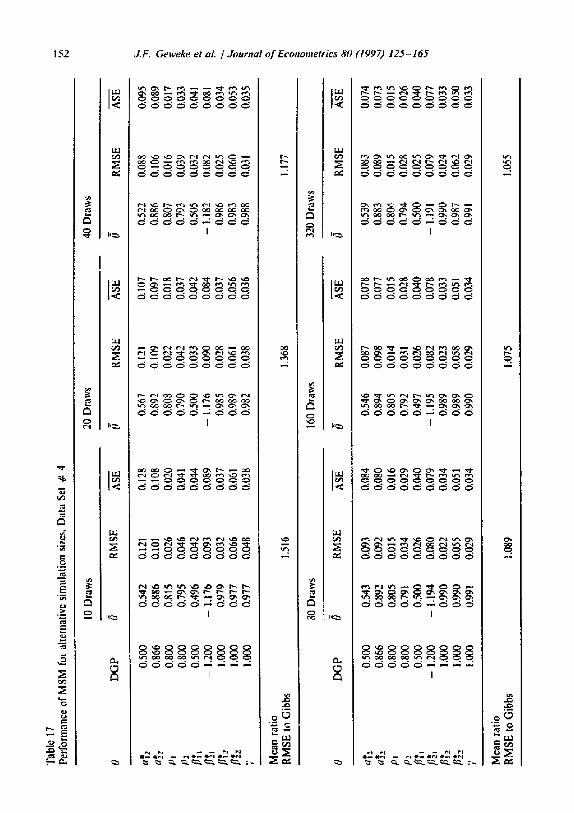
6.2. Experiment 2 - - effect o f simulation size
In this exper iment we consider the effect of the n u m b e r of draws used to construct the G H K s imula tor on the per formance of M S M and SML. In particular, we want to determine whether the generally higher RMSEs for S M L and MSM, relative to GIBBS, can be a t t r ibuted to an insufficient number of draws in the G H K algori thm. Thus, we consider M S M and S M L es t imators implemented using G H K simulators based on I0, 20, 40, 80, 160, 320, 640 and 1280 draws.
It is impract ical to repeat the analysis using all 12 da ta structures used in exper iment 1 and all 8 al ternat ive simulat ion sizes. Instead, we use the two data structures that generate the lowest and highest R M S E s for S M L and MSM, relative to GIBBS. The last eight rows of Table 13 indicate that the best case for the classical es t imators relative to G I B B S is da ta s tructure # 9, with low serial corre la t ion in disturbances, high serial correlat ion in regressors, and high cross correlat ion in disturbances. Conversely, the worst case for S M L and M S M is data s t ructure ~ 4, in which these correlat ions are high, low, and low, respec- tively.
in Table .~4 we repor t the results for SML, using the same 20 artificial da ta sets generated with da ta s tructure # 9 as were used in exper iment 1. For each s imulat ion size, we also repor t the average (across parameters) o f R MSE relative to that for the G I B B S est imates based on m = 5000 iterations. We do this because s tandard methods for evaluat ing the accuracy of poster ior momen t s (see Geweke, 1992) indicate that, with an = 5000, further G ibbs i terations should produce negligible changes in RMSE. Thus, the RMSEs for G I B B S provide a reasonable benchmark.
The Tab le 14 results are roughly consmtent with the convent ional wisdom reported in Br rsch-Supan and Hajivassiliou (1993) that S M L based on G H K performs w e , using only 20 draws. The mean across all 9 model parameters of
J.F, Geweke et al. / Jovrna l o f Econometr ics 80 (1997) 1 2 5 - 1 6 5 145
T a b l e 13 R o o l m e a n s q u a r e e r r o r c o m p a r i s o n
C o v a r i a t e P r e d i c t e d R M S E
Coeff. S td E r r t - r a t io
I n t e r c e p t -- 3.633 0.064 -- 56.493 M S M - G H K O. 165 0.090 1.846 S M L - G H K 0.043 0.090 0.483
Corrf~ht , ~12,) = 0.80 x D E P = R H O 0.051 0.049 1.O43
Pt = P2 = 0.80 × D E P = R H O - 0.421 0.049 - 8.615 $ 2 = 0.50 × D E P = R H O - 0.383 0 .060 -- 6.409 ~b 2 = 0.80 x D E P = R H O - 0.530 0.060 - 8.864
a*2 x M S M - G H K 0.103 0.105 0.980 a*2 x M S M - G H K - 0.047 0,105 - 0.447 p~' x M S M - G H K -- 0.021 0-105 - 0.196
p~ × M S M - G H K - 0 .034 0,105 - 0,326
fll*t x M S M - G H K - 0.015 0.105 - 0 ,140 fl~, x M S M - G H K 0.061 0 . t 0 5 O,57a
fit*_, x M S M - G H K --O.181 0.105 -- 1,713 /J*, x M S M - G H K - 0.195 0.105 -- 1.852
aT2 x S M L - G H K 0.191 0.105 1.812 a ~ × S M L - G H K 0.280 O. 105 Z 6 5 0
p* x S M L - G H K 0.767 0.105 7.274
p* x S M L - G H K 0.909 0.105 8.62 I [l[t x S M L - G H K 0.110 0.105 i .043 / ~ t x S M L - G H K 0,108 0.105 ! .028 fl~'2 x S M L - G H K - 0.046 0.105 -- 0.434 tJ~2 x S M L - G H K - 0.167 0.105 - 1.585
C o r r P h , , ~lz,) = 0.80 x M S M - G H K - 0.082 0.050 - 1.652 Pt = Pz = 0.80 × M S M - G H K 0.129 0.050 2.597 ~b ~ -- 0.50 x M S M - G H K 0.033 0.061 0.543 ~b 2 = 0.80 × M S M - G H K - 0.057 0.061 - 0.938
C o r r i r h , , ll2t) = 0.80 x S M L - G H K - 0.129 0.050 - 2.585 PL ---- P2 = 0.80 x S M L - G H K 0.142 0.050 2.865 ~b z = 0.50 × S M L - G H K - O.G18 0.061 - 0,292
q~-" = 0.80 × S M L - G H K - 0.148 0.061 - 2.431
Note : D e p e n d e n t va r i ab l e is Iog (RMSE) . D E P = R H O m e a n s t ha i the d e p e n d e n t va r i ab l e fo r tho
o b s e r v a t i o n is t he I o g ( R M S E ) for a p a r a m e t e r p l o r p_,. c~., = p j ~ . , - ~ + fit, c2., = P ,~2 . , - t + t/_,, t:a. ~ ~ 0 .
Tab
le 1
4 Pe
rfor
man
ce o
f SM
L f
or a
lter
nati
ve s
imul
atio
n si
zes,
Dat
a Se
t #
9 z~
10 D
raw
s 20
Dra
ws
0 D
GP
~
RM
SE
ASE
0
RM
SE
ASE
tJ
a]'2
0,
800
0.75
2 0.
094
0.06
6 a'~
z 0,
600
0.67
3 0.
087
0.05
2 p~
0,
500
0.45
6 0.
052
0.02
3 P2
0.
500
0.41
1 0.
101
0,03
8 flT
~ 0.
500
0.50
0 0,
025
0,02
9 fl
~
- 1.
200
- 1.
254
0,11
6 0,
090
//1,:
1.00
0 0.
983
0,03
6 00
38
flC_z
1.00
0 0.
965
0,07
3 0.
061
7 1.
000
1.01
2 0,
045
0.03
9 M
ean
rati
o R
MSE
to
Gib
bs
1.31
0
40 D
raw
s
0.76
2 0.
081
0,07
2 0,
788
0.63
4 0.
064
0.05
2 0,
616
0A73
0.
037
0.02
4 0,
487
0.44
4 0.
072
0.04
0 0.
456
0A99
0.
027
0,03
0 0,
500
- 1.
212
0.10
3 0,
091
- 1.
190
0.98
2 0.
037
0,03
9 0.
981
0,95
9 0.
070
0.06
3 0,
963
1.00
1 0.
042
0.04
1 0.
992
1.09
3
80 D
raw
s
RM
SE
ASE
0,07
2 0.
078
0.05
5 0.
051
0,02
7 0.
024
0.06
1 0.
041
0.02
6 0.
030
0.09
9 0.
094
0.03
7 0.
040
0.06
7 0.
065
0.03
9 0.
042
0.97
!
160
Dra
ws
l~
DG
P
0 R
MSE
A
SE
~ R
MS
E
ASE
/~
320
Dra
ws
RM
SE
A
SE
aTz
0,80
0 0.
779
0.07
3 0.
083
0,79
0 0.
069
0.08
6 0.
770
0.08
4 a.,
*2
0.60
0 0.
599
0.05
2 0.
052
0.59
1 0,
054
0.05
3 0.
582
0,05
4 p~
0,
500
0.49
6 0.
024
0.02
4 0.
499
0.02
5 0,
024
0500
0,
024
p..
0,50
0 0.
476
0,04
9 0.
041
0.48
2 0.
050
0.04
2 0A
85
0,04
8 /J
~ 0,
500
0.49
5 0~
027
0,03
1 0.
496
0.02
7 0.
031
0A94
0,
026
/J*.~
-
1,20
0 -
1.17
9 0.
104
0.09
6 -
1.17
2 0,
103
0.09
7 -
1.16
1 0.
101
/J~'~
1,
000
0.97
9 0.
038
0.04
1 0.
981
0,03
8 0,
041
0,98
1 0,
037
[J~.
t.0
00
0.96
t 0.
065
0.06
9 0.
965
0,06
9 0.
070
0.95
8 0,
067
7 1.
000
0.98
9 0.
044
0,04
3 0.
987
0,04
2 0.
043
0.98
7 0.
043
Mea
n ra
tio
RM
SE
to
Gib
bs
0.94
9 0.
944
0,94
9
0.08
6 0.
053
0.02
4 0.
043
0.03
1 0.
097
0.04
1 0.
072
0.04
3
I
640
Dra
ws
1280
Dra
ws
,1L-
Pt t-2
? Mea
n ra
tio
RM
SE
to
Gib
bs
DG
P
RM
SE
ASE
I~
R
MS
E
ASE
0.80
0 0,
779
0.06
6 0,
089
0.78
2 0.
600
0,58
3 0.
056
0.05
3 0.
582
0.500
0.503
0.025
0,024
0.502
0.50
0 0.
487
0.04
6 0.
043
0.48
6 0.
500
0A94
0.
027
0.03
1 0.
494
- 1.
200
- 1.
161
0.10
6 0.
098
- 1.
162
1.00
0 0.
980
0.03
8 0.
042
0.98
1 1.
000
0.96
2 0.
065
0.07
1 0.
964
1.000
0.985
0.04
3 0.044
0.985
0.072
0.089
0.056
0.053
0.025
0.024
0.O43
0.O43
0.027
0.031
O. 1
05
0.O
98
0,037
0.04
2 0.064
0.07
1 0.043
0.04
4
0.939
0.93
1
e~
.,,.. ,% 8
Tab
le
15
Per
fom
lane
e of
MS
M f
or a
ltern
ativ
e si
mul
atio
n si
zes.
Dat
a Se
t #
9
10 D
raw
s
0 D
GP
0
RM
SE
ASE
a~'2
0,
800
0,74
6 0.
116
0.14
6 aL
, 0,
600
0,57
4 0,
064
0.06
1 th
0.
500
0,50
5 0,
034
0.02
8 p.
, 0.
500
0,49
4 0,
061
0.05
2 [IT
~ 0.
500
0.49
2 00
31
0,03
2 ~
t -
1,20
0 -
1.15
5 0.
097
0.11
3 B
~':
1,00
0 0,
980
0.03
7 0.
043
11~2
LO
00
0.94
6 0.
080
0.08
9 7
1.00
0 0.
989
0.1)
44
0.04
6 M
ean
rati;
, R
MS
E t
o G
ibh~
i.
i 15
20 D
raw
s 40
Dra
ws
RM
SE
ASE
~
RM
SE
ASE
0.79
9 0,
080
0,12
7 0.
778
0,58
6 0.
057
0,05
9 0.
586
0.50
6 0.
026
0.02
6 0.
504
0.48
0 0.
061
0.04
9 0.
48t
0,49
6 0.
026
0.03
2 0A
97
- 1.
165
0.09
8 0.
109
- 1.
160
0.98
3 0.
038
0,04
3 0.
984
0.96
9 0.
070
0,08
3 0.
963
0.98
5 0.
043
0,04
5 0.
986
0.99
5
80 D
raw
s
0.07
3 0.
! 09
0.05
9 0,
057
0.02
5 0,
025
0.05
6 0.
045
0.02
8 0.
03 I
0.10
5 0.
106
0.03
7 0.
042
0.06
6 0.
077
0.04
3 0.
044
0.98
2
160
Dra
ws
320
Dra
ws
0 D
GP
0
RM
SE
ASE
~
RM
SE
A
SE
RM
SE
ASE
aT:
0.80
0 0.
795
0.08
0 0.
099
0.78
6 0.
078
0.09
4 0.
785
0.06
3 n.
,*:
0.60
0 0.
585
0,06
2 0~
054
0,58
1 0.
055
0.05
4 0.
585
0.05
5 pj
0.
500
0.50
7 0.
026
0.02
5 0.
505
0.02
5 0.
024
0.50
4 0.
024
p,
0.50
0 0.
489
0.05
1 0.
043
0.48
9 0.
047
0.04
2 0.
488
0.04
6 fl*
~ 0,
500
0.49
6 0.
028
0.03
1 0.
495
0.02
7 0.
031
0.49
5 0.
027
[l~:
- 1.
200
- 1,
169
0.10
8 0.
102
- 1.
165
0.10
I 0.
101
- 1.
168
0.10
6 fiT
: 1.
000
0.98
3 0.
037
0,04
2 0.
983
0,03
7 0.
042
0.98
3 0.
037
[l',,_
1.
000
0.97
1 0.
065
0,07
4 0.
969
0.06
3 0.
073
0.96
7 0.
064
;, 1.1
300
0.98
6 0.
042
0.04
4 0,
987
0,04
3 0,
043
0.98
8 0.
043
Mea
n
rati
o R
MS
E l
o G
ibbs
0.
984
0.94
2 0.
924
O.0
9]
O.0
54
0.O
24
0.04
1 0.
031
0.10
0 0.
042
0.07
2 0.
043
t.,.,
.-,7
$ I
640
Dra
ws
1280
Dra
ws
m
0 D
GP
0
RM
SE
ASE
~'~
R
MSE
A
SE
aI'2
0.
800
0.78
4 0.
069
0.08
9 0.
784
0.06
7 a[
z 0.
600
0.58
4 0.
056
0.05
3 0.
585
0.05
5 Pt
0.
500
0.50
4 0.
024
0.02
4 0.
504
0.02
5 p_
, 0,
500
0.48
7 0.
045
0.04
1 0.
487
0.04
6 //~
*~
0.50
0 0.
495
0.02
7 0.
031
0.49
5 0.
027
//*~
- 1.
200
- 1.
166
0.10
7 0.
100
- 1.
167
0,10
5 //
'2
1.00
0 0.
983
0.03
6 0.
042
0.98
3 0.
036
~,
1.00
0 0.
967
0,06
4 0.
071
0.96
7 0.
064
7 1.
000
0.98
7 0.
043
0.04
3 0.
987
0.04
3
Mea
n ra
tio
RM
SE
lo
Gib
bs
0.93
1 0.
931
0.08
9 0.
053
0.02
4 0.041
0.031
0,I0
0 0.
042
0.071
0.04
3
n~
",O
I m ,g
Tab
le 1
6 Pe
rfor
man
ce o
f S
ML
for
alte
rnat
ive
sim
ulat
ion
size
s. D
ata
Set
# 4
10 D
raw
s
0 D
GP
O
R
MSE
A
S-E
/~
a'/z
0,50
0 0.
631
0.15
0 0.
064
a~2
0.86
6 1.
042
0.18
9 0.
064
Pl
0.80
0 0.
719
0.08
3 0.
015
p,_
0.80
0 0.
617
0,18
9 0.
028
//'/t
0.
500
0.50
3 0,
024
0.03
0 //~
t -
1.20
0 -
i.237
0.
075
0.07
0 //~
'2
1,00
0 0.
997
0,02
3 0.
029
//*'.2
1.
000
1.01
6 0.
061
0.04
5 "7
1.
000
i .00
0 0.
029
0.02
9 M
ean
ratio
R
MSE
Io
Gib
bs
2,34
5
20 D
raw
s 40
Dra
ws
RM
SE
A
SE
0 R
MSE
A
SE
0.62
0 O
. 138
0.
067
0.60
6 1.
012
0.16
1 0,
064
0.98
7 0.
755
0.04
8 0.
014
0.77
5 0.
680
0.12
4 0.
027
0.71
7 0.
499
0.03
0 0.
033
0.49
7 -
1.21
8 0.
062
0,07
0 -
1.20
7 0.
990
0.02
3 0,
030
0.98
9 1.
003
0.05
7 0.
0/16
0.
999
0.99
1 0.
025
0.03
0 0.
990
1.79
1
80 D
raw
s
0.12
5 0.
069
0.14
2 0.
066
0,02
9 0.
014
0.08
7 0.
026
0.02
8 0.
035
0.06
9 0.
072
0.02
4 0.
031
0.05
0 0.
046
0.02
8 0.
031
1,47
3
160
Dra
ws
0 D
GP
0
RM
SE
ASE
0
RM
SE
ASE
320
Dra
ws
RM
SE
ASE
a*z
0.50
0 0.
579
0,09
7 0.
069
0.54
7 0,
076
0,06
8 0.
550
0,08
4 a~
'2
0.86
6 0.
947
0.11
2 0.
066
0.91
4 0.
089
0.06
7 0.
905
0.08
3 P
l 0.
800
0.78
7 0.
021
0.01
4 0.
795
0.01
6 0.
014
0.79
8 9.
015
P2
0.80
0 0.
752
0.05
5 0.
025
0.77
3 0.
042
0.02
5 0.
778
0.03
5 //'
/i 0.
500
0.49
8 0.
024
0,03
7 0.
497
0.02
8 0.
038
0.49
7 0.
024
//~
-
1.20
0 -
1.12
0 0,
071
0,07
3 -
1,19
4 0,
065
0.07
4 -
1,18
8 0,
071
/1'/,
1,
000
0.99
0 0.
025
0.03
1 0,
989
0,02
4 0,
032
0.98
8 0.
025
//.,*
2 i.0
00
0.99
3 0.
056
0.0-
¢.7
0.98
9 0.
051
0.04
7 0.
98 '~
0.
'x'~
6 7
1.00
0 0.
992
0.03
0 0.
031
0.98
9 0.
032
0.03
2 0.9
Q.v,
0.
0."0
Mea
n ra
tio
RM
SE
to
Gib
bs
1.22
2 1.
073
1.05
2
0.07
1 0.
068
0.01
4 0.
025
0.03
8 0.
074
0.03
2 0.
047
0.03
2
+ e.,
.,.., i t,m
640
Dra
ws
1280
Dra
ws
0 D
GP
f~
R
MSE
A
SE
~ R
MS
E
ASE
aT2
0.50
0 0.
544
0.07
5 0.
072
0.53
9 0.
072
a~
0.86
6 0.
897
0077
0.
069
0.89
0 0.
079
Pl
0.80
0 0.
801
0.01
4 0.
014
0.80
0 0.
013
Pz
0.80
0 0.
787
0.02
8 0.
026
0.78
9 0.
029
//]'~
0.
500
0.49
6 0.
025
0.03
9 0.
497
0.02
6 fl
~l
- 1,
200
- 1.
193
0.07
2 0,
075
- 1.
189
0.07
2 fiT
., 1.
000
0.98
8 0.
024
0.03
2 0.
989
0.02
3 /~
_,'2
1.00
0 0.
988
0.05
6 0.
047
0.98
7 0.
056
;, 1.
000
0.98
9 0.
030
0.03
2 0.
989
0.02
9
Mea
n ra
tio
RM
SE
to
Gib
bs
1.00
0 0.
994
0.07
2 0.
070
0.01
5 0,
025
0.03
9 0.
075
0.O
32
O.O
47
0.03
2
,-,.
Oc I C,,
Tab
le 1
7 Pe
rfor
man
ce o
f M
SM
for
alte
rnat
ive
sim
ulat
ion
size
s, D
ata
Set
# 4
10 D
raw
s 20
Dra
ws
0 D
GP
(~
R
MSE
A
$-'--E
O
R
MSE
A
SE
40 D
raw
s
RM
SE
ASE
aT2
0.50
0 0.
542
0.12
1 0.
128
0.56
7 0.
121
0.10
7 0.
522
0.08
8 a*
, 0.
866
0.88
6 0.
101
0.10
8 0.
892
0.10
9 0.
097
0.88
6 0.
106
p~
0.80
0 0.
815
0.02
6 0.
020
0.80
8 0.
022
0.01
8 0.
807
0.01
6 P2
0.
800
0.79
5 0.
046
0.04
1 0,
790
0,04
2 0,
037
0.79
3 0.
039
fl*t
0.
500
0.49
6 0.
042
0.04
4 0.
500
0.03
3 0.
042
0.50
5 0.
032
fl,*=
-
1200
-
1.17
6 0.
093
0.08
9 -
t.176
0.
090
0.08
4 -
1.18
2 0.
082
[l'{z
1.00
0 0.
979
0.03
2 0.
037
0.98
5 0.
028
0.03
7 0.
986
0.02
5 [l~
z 1.
000
0.97
7 0.
066
0.06
1 0.
989
0.O
61
0.05
6 0.
983
0.06
0 7
1,00
0 0.
977
0.04
8 0.
038
0.98
2 0.
038
0.03
6 0.
988
0.03
1
Mea
n ra
tio
RM
SE
la
Gib
bs
1.51
6 1.
368
1.17
7
,~0
Dra
ws
160
Dra
ws
320
Dra
ws
0 D
GP
~
RM
SE
ASE
O
R
MS
E
ASE
0.09
5 0.
089
0.O
I7
0.03
3 0.
041
0.08
1 0,
034
0,05
3 0.
035
RM
SE
ASE
a*,_
O.5
00
0.54
3 0.
093
0.08
4 0.
546
0.08
7 0.
078
0.53
9 0.
083
a*z
0.86
6 0.
892
0.09
2 0.
080
0.89
4 0.
098
0.07
7 0.
883
0.08
9 pt
0.
800
0.80
5 0.
015
0.01
6 0.
805
0.01
4 0.
015
0.80
4.
0.01
5 p
, 0.
800
O.7
9t
0.03
4 0.
029
0.79
2 0.
031
0.02
8 0.
794
0.02
8 fl
'/,
0.50
0 0.
500
0.02
6 0.
040
0.49
7 0.
026
0.04
0 0.
500
0,02
5 /./
~ -
1.20
0 -
1.19
4-
0.08
0 0.
079
- 1.
195
0.08
2 0.
078
- 1.
191
0.07
9 ~
'z
1.00
0 0.
990
0.02
2 0.
034
0.98
9 0.
023
0.03
3 0.
990
0.02
4 ~.
-*z
t.000
0.
990
0.05
5 0.
051
0.98
9 0.
058
0.05
1 0.
987
0.06
2 ,,
t.000
O
.991
0.
029
0.03
4 0.
990
0.02
9 0.
034
0.99
1 0.
029
Mea
n ra
tio
RM
SE
to
Gib
bs
1.08
9 I.O
75
1.05
5
0.074
0.073
0.015
0.026
0.040
0.077
0.033
0.050
0.033
.=.,
t,,,, _=
0¢, 1 ,..
,.,
640
Dra
ws
1280
Dra
ws
0 D
GP
~
RM
SE
AS---
-F
0 R
MSE
A
St~
aT,,
0.50
0 0.
540
0.08
0 0.
072
0.54
1 0.
079
a*,z
0.
866
0.88
7 0.
086
0.07
2 0.
890
0.08
4 Pl
0.
800
0.80
3 0.
014
0.01
5 0.
802
0.01
4 P2
0.
800
0.79
3 0.
028
0.02
5 0.
791
0.02
8 fl
i't
0.50
0 0.
500
0,02
6 0.
039
0.50
0 0.
025
fl~,
-
1.20
0 -
1.19
4 0,
077
0.07
7 -
t.192
0.
074
flT.~
1.
000
0.99
0 0.
023
0.03
3 0,
990
0.02
3 /J
~,
1,00
0 0.
990
0.05
8 0,
049
0.99
0 0,
058
7 1.
1300
0,
991
0.02
9 0.
033
0,99
1 0,
029
Mea
n ra
tio
RM
SE t
o G
ibbs
!.0
33
1.01
7
0.071
0.071
0.015
0.025
0.039
0,077
0,033
0.049
0.033
p,.. a~
',,.n
I
154 J.F. Geweke et aL /Journal o f Econometrics 80 (19971 125-165
the RMSE for SML is only 9% greater than GIBBS, and agreement between RMSE and ASE is generally good. The exceptions are Pt and p2, for which downward bias is noticeable and RMSEs are well above ASE. Noticeable improvements in RMSEs and in agreement between RMSEs and ASEs for the autoregressive parameters are achieved by increasing the number of draws to 49 or 80, but little is gained by going beyond that.
Note that for the slope parameters fl* and "2 there is little change in RMSE in going from 20 (or even 10) up to 1280 draws. Thus, the conventional wisdom that "20 draws is enough" may well stem from th: tendency to focus on such parameters to the exclusion of the covariance structure parameters (in fact, recall that B6rsch-Supan and Hajivassiliou (1993) held the covariance structure parameters fixed at true values in their study}. But clearly, i ra M M P mn,~ ,1 is to be used to model behavior, then the covariance parameters are every bit as important as the slope parameters.
The MSM results for data structure # 9 are reported in Table 15. When only 20 draws are used MSM performs even better than SML. The mean across all nine model parameters of the RMSE is essentially identical to that for GIBBS, and the agreement between RMSE and ASE is generally good. in contrast to SML, no downward bias is apparent for Pt and P2, even when only 10 draws are used. This is consistent with findings in Keane (1994). Again, it appears that increasing the number of draws beyond 20 leads to only minor improvements in RMSEs.
In Table 16 we report the results for SML using data structure # 4 - the worsl ease for MSM and SML. These results sharply contradict the conven- tional wisdom that '20 draws is enough'. Using only 20 draws, the mean RMSE for SML is roughly 79% greater than for GIBBS. Biases for all the covariance parameters are severe, especially for pt and P2. 160 draws are needed to reduce the RMSE for SML to less than 10 percent greater than GIBBS, and 640 draws are needed to reduce it to the same level as for GIBBS. But even here, for the slope parameters it appears that the i m p r o v c ~ n t s in RMSE that are achieved by going past 20 draws are minor.
The MSM results for data structure # 4 arc reported in Table 17. The performance of MSM in this worst case is much superior to that of SM L. Using 20 draws, the mean RMSE for MSM is roughly 37% greater than for GIBBS. This is much better than the 79% figure achieved by SML. Even more impor- tantly, there is no evidence of bias, even when only 10 draws are used. This is again consistent with findings in Keane (1994).
7. Conclusion
We have compared the sampling properties of the GIBBS estimator obtained by using Gibbs sampling and data augmentation to compute posterior means,
d.F. Geweke el al. / Journal o f Econoraetrics 80 0997) 125-165 155
the MS1H estimator using the G H K probability simulator, and the SML estimator using the G H K probability simulator. In a controlled Monte Carlo experiment we find that all three estimators perform reasonably well in point estimation of parameters of the data generating process in a three alternative 10-period multi- hernial multiperiod probit model. However, the relative performance of the methods varies as we vary the treatment variables in our experimental design.
Four important patterns emerge in the response of RMSEs to the design variables. First, RMSEs for all estimation methods and model parameters rise as serial correlation in either the errors or in the covariates is increased, except for the AR(I) parameters, for which RMSEs fall. Second, RMSEs of the SML and MSM estimates rise substantially relative to those of the GIBBS estimates as serial correlation in the errors increases. Third, increasing serial correlation in the covariates leads to a small relative decrease in the RMSEs of the SML estimates. Fourth, increasing cross correlation of the errors leads to relative declines in the RMSEs of the SML and MSM estimators.
Of these patterns, we feel that the most important to a user of these methods is the fact that, holding draws fixed, both the relative and absolute performance of the classical methods, especially SML, becomes worse as serial correlation in disturbances increases. In data sets with an AR(I )parameter of O.50, the RMSEs for SML and MSM based on 20 draws exceed those oFGIBBS by 9% and 0°A, respectively. But when the AR(I) parameter is 0.80, the RMSEs for S ML and MSM based on 20 draws exceed those oFGIBBS by 79%0 and 37%, respectively, and the number of draws needed to reduce the RMSEs for S ML and MSM to within 10% of GIBBS are 160 and 80, respectively.
In existing applications it is common for MSM or SML to be implemented using G H K simulators based on only 10 or 20 draws, and conventional wisdom seems to suggest that 20 draws is "enough'. But our results suggest that when serial correlation in the errors is strong, substantial RMSE reductions can be achieved by going to 80 or 160 draws. And in the case of SML, substantial bias reductions can be achieved as well. The main weakness of SML relative to the other methods is in estimation of serial correlation parameters. When 20 draws are used, the SML estimates of the AR(I) coefficients are clearly biased down- ward and have RMSEs roughly twice as great as for o ther methods. This problem would lead to larger RMSEs in out of sample forecasts obtained using SM L as compared to the other methods. It appears that from 80 to 320 draws must be used in order to render these biases insignificant.
For purposes of statistical inference it is desirable that ASE or PSD be similar to RMSE. There is generally close agreement between RMSEs and ASEs for MSM, and somewhat less close but still acceptable agreement between RMSEs and PSDs for GIBBS. But, when only 20 draws are used, RMSEs of SM L point estimates exceed ASEs by 38% on average. This divergence is greater when serial correlation in errors is strong, and it can be reduced by using more draws.
156 J.F. Geweke el aL /Journal o f Econometrics 80 (1997) 12S-165
What accounts for the increases in RMSEs for MSM and SML relative to GIBBS as serial correlation in the errors is increased while holding simulation size fixed? It stems from the different roles of simulation in the estimators. In MSM and SML, a set of nonlinear equations is solved iteratively. Equation evaluation at each i teration is approximate, but consistent in the number of G H K draws. As serial correlation increases, more draws are needed to maintain a given level of accuracy of the G H K approximation. In GIBBS, simulation- consistent approximat ion of posterior means comes about because, over the whole set of iterations, the simulator draws a sample representative of the posterior distribution. With increased disturbance serial correlation, a greater number of iterations is required to achieve a representative sample because the Gibbs sampler navigates the posterior more slowly. Thus, performance of each method should deteriorate as serial cotrelation in disturbances is increased, but the relative rate of deterioration is an empirical question. In our experiments, 5000 iterations of the Gibbs sampler provides good approximations to the posterior for both high and low degrees of serial correlation. In contrast, 20 draws for the G H K simulator provides comparable approximation accuracy when serial correlation is low, but the number must be made much greater when serial correlation is high.
Since we argue that RMSEs of the MSM and SML estimators based on G H K with 20 draws and GIBBS posterior means based on 5000 Gibbs iterations are similar when serial correlation is relati'~'ely weak (i.e., AR(I) parameters in the 0.50 range}, but that roughly 80 to 320 draws for MSM and S ML are needed to maintain comparable performance when serial correlation is strong 0.e., ARO) parameters in the 0.80 range}, it is important to consider how computat ion time for the various methods is affected by simulation size.
Unfortunately, it is essentially impossible to give absolute time comparisons for these methods for several reasons. For example, since most of the computa- tion time for GIBBS is used in drawing the latent utilities, time for GIBBS increases slowly as the number of model parameters increases. But for SM L and MSM, computat ion time is roughly proport ional to the number of parameters, since most of the time in these methods is spent calculating derivatives and the initial weighting matrix, respectively. Also, relative timings for the methods wilt depend on the number of iterations necessary to achieve convergence for the classical methods, and the number of Gibbs iterations needed to achieve a de- sired level of numerical accuracy. In particular, for MSM the calculation of the initial weighting matrix is much more time consuming that subsequent iter- ations, while for SML all iterations take roughly equal time. And the number of iterations needed for convergence is particular to the application at hand. Finally, if one wishes to check sensitivity of results to simulation size, MSM and SML require that one redo the entire estimation ~,sing more draws, while with GI BBS one can simply restart the algorithm from end values and add additional iterations. Thus, monitoring numerical accuracy is much easier with GIBBS.
J.F. Geweke et al. / Journal o f Econometrics 80 (1997) 125-165 157
Despite these problems, it is informative to give so,.-ne timing information based on our Monte Carlo experiments. The typical t ime for our GIBBS runs on an IBM 3090 mainframe was 816 cpus. Timings for the classical methods is much more variable than for GIBBS, because the number of iterations needed to achieve convergence varies greatly across Monte Carlo data sets. On average, the number of iterations needed to achieve convergence for the data sots considered here is about I0. For SML, a regression of computat ion time per iteration on number of draws produced the result 5.2 + 0.74*Draws. Thus, the predicted times for ten iteration runs using 20, 80 and 160 draws arc 200, 644 and 1236 epu s, respectively. For MSM, a regression of marginal computat ion time per iteration on number of draws produced the result 2.7 + 0.54*Draws, while a regression of initial weighting matrix computat ion time on number of draws produced the result - 2.0 + 3.44*Draws. Thus, the predicted times for ten iteration runs using 20, 80 and 160 draws are 202, 732 and 1439 cpu s, respectively. We interpret these results as indicating that computat ion times are in the same ballpark for all three methods, given models of the size considered here and simulation sizes of the type one would typically employ. Thus, we conclude that computa t ion time should not be a decisive factor in choosing among the methods.
If we had found that computat ion times for G1BBS greatly exceeded those Ior MSM or SML, it would make sense for a Bayesian practi t ioner to consider these methods as a way to approximate posterior means. That this is not the case implies that a Bayesian should have no interest in these alternatives - provided that Gibbs sampling data augmentat ion software is at hand.
Appendix A: application of the GHK simulator to the MMP model
Here we provide a description of the G H K simulator as applied to the simulation of choice probabilities in the M M P model described in Section 2. F o r a proof of the unbiasedness of the G H K simulator in genera l see B~rsch-Supan and Hajivassiliou (1993). To describe the G H K simulator it is useful to define some additional notation. Let
0,'/~, = Ui*+ U~, ( j = 1, , J ; t = 1 . . . . . T), ~,~, * * - - • * • - - ~ ~ [ k r - - l ; i j l -
(Notice that L?~j+ = 0 and ~j, = 0.) Choice j is made at t if the J -- I constraints O~k, < 0 for all k # : j are satisfied. Fur ther let
where d+ is the choice vector defined in (2.4). Thus +(d, +) -- IIDN(0, ~(dl)), where ~(d+) is the appropriate transformation of 27".
158 J.F. Geweke et al. / Journal o f Econometrics 80 (1997) 125-165
Le t ~(d~) be the u n i q u e l o w e r t r i a n g u l a r C h o l e s k y d e c o m p o s i t i o n -if(d;) = ~(d~) ~(dr) ' . T h e n g(d;) = / ~ ( d i ) ~q(di), w h e r e ( s u p p r e s s i n g the i s u b s c r i p t ) ~,( - j , ) = (ri], . . . . . rb, _ ,.,, tlj, + ,., . . . . . rij,)', q (d , ) = ( # , ( - - j , ) . . . . . q r ( - - J r ) ) ' , a n d rhjs "~ I D N ( 0 , I) fo r all i , j , t.
Fina l ly , de f ine - 1 -r ~ . , - t . . . . U i , , ( r / t l . . . . . . r~ , , ~ , ) a s t h e v a l u e o f £7~,t w h e n t h e r a n d o m v a r i a b l e s (ri~] . . . . . q J . , - ~ , q t , . . . . . ~p,) a r e f ixed a t the d r a w (0~,, ,q~ , ,q' , , -, . . . . , - . . . . r/pt). N o t e t h a t fo r p = k th is is a n u m b e r , a n d fo r p < k th is is a r a n d o m va r i ab l e . T h e n , t he G H K s i m u l a t o r for t h e p r o b a b i l i t y o f t h e c h o i c e s e q u e n c e ( d i t , - - . ,d,-t), o r e q u i v a l e n t l y ( j l t , . . . ,Jlt), is c o n s t r u c t e d as fo l lows ( s u p p r e s s i n g the i subsc r ip t ) :
P e r i o d 1:
Step:
(J)
P e r i o d t. Step:
(1) D r a w r/tit s.t. OJi l ( ; / I t l ) < 0
( j ~ - 1)Draw r/~,_ ,., s.t. /.7~',,_ t . t ( t f t t , . . . , r / J , _ n., ) . < 0
( j~) S k i p ~/J.,~
( j , + 1 ) D r a w J/,~, +,. , s.t. 0~',, +, . , o / t t , . . . . ,t7~, , . , , t/I, + ,.,) < 0
D r a w r/~t, s.t.t..79 t ( r f t , . . . . . t/J, _ , . , , t7~ ' + ,., . . . . . qS, ) < O
(1) D r a w 'l~, s.t. 0 ~ i , ( ~ t fit . . . . . t j . , - 1 , q t n ) < 0
(.fi - 1) D r a w ~l~. - ,., s.t. 0'~',._ 1.,(ri~ ~ , . . . , ~ t . _ , , ~ , . . . . , rb _ 1 . , ) t < 0
l j,} Skip ~,, ( . b + 1) D r a w 0~;. , . , s.t. Oj;+ ,.,(qJt~ . . . . . $ ~ . , - , , tft . . . . . . t/~_,.1, r / J , + , . , ) < 0
/~r , rl/lt . . . . t 1 (d) D r a w r/~, s.t. O$,(0~1, .-. • D . , - t , tb .- L,, qj. + ,.,, . . . . q~,) < 0
a n d f inal ly, c o n s t r u c t :
P G . K ( d t . . . . . d, l l l* , Z * . X * ~
1 M j , -
= Mt~t= P(G'~ ' t < O) k=-,I'] e [ O ~ t ( t i ~ t ] . . . . . t / I_ [ . , ) < 0]
J.F. Geweke et al. /Journal o f Econometrics 80 (1997) 125-165 159
- - A ! x P [ U j , + ,.L(~l~l < . . . . . ~j,- L,) O] J
Appendix 13: a Gibbs sampling data augmentation algorithm for tke M M P model
In order to describe the Gibbs sampling da ta augmenta t ion algori thm, it is first useful to define the proper pr ior distributions in generic notation:
~ "" N(I~7, V~7) ( j -~ 1 . . . . . J -- 1)
7 "-- N(y, V;.)
pj ... TN(ppa~,) ( j = 1 . . . . . J - I),
where T N denotes t runcat ion of the univariate normal distribution to the unit interval (0, 1);
~ , , - t ~ W ( S - t ; v ) ,
where W denotes the Wishart distribution. These priors are assumed mutual ly independent.
It is also useful to adop t the notat ional convent ion U~'o = ~*o, )~'o = [O1, Z*o = [0], and to define three equivalent expressions for the probabil i ty density kernel of the U*, which are
IVJi-sr/2exp ---~ ~" (e.~ - - R ~ * , _ , ) ' ~ P - ' ( ~ * - - R ~ * , - , ) , (B.I) i = t t = l
where ~* = U~ - X * [f* - Z * 7 ; or
x ~ - ' ( 0 ~ , - .~*~* - -2"7)~ , (B.2)
1
J
160 J.F. Ge~w.ke et al. / Journal o f Econometrics 80 (1997) 125-165
where
0 7 , = v ~ , - R u * , _ ~ ,
and
. ~ =.,L*, - RY,~. ,_i . 2,*, = z~, - R z ? . , _ , ;
I~PI-Nrt2exp - - ~ [ U ~ -- R U * , _ : -- (p~, - - R/a~.,_I) ] ~ - t i = l I = l
x [ U ~ - - R U * , _ , - - {#,, - R/t,.,_, ) ]~ , (B.3)
where Pit = X * f l * + Z ~ 7, each multiplied by the kernel density of the uncondi- tional distribution of ~,*o,
[ Vo(R, ~ ) [ - N/Z exp - ~ ,~ , r.,-*o [ V o ( R , ~ ) ] - ' ~*o ~, (B.4)
where [Vo(R, ~)]j~ = ¢~d(1 - PjPD.
The kernel of the posterior density function for fl*, 7, P, ~, and the U* is the product of(B.I) or (B.2) or (B.3); (B.4); the density kerr,~;is for the prior distribu- tions; and
N T
I-I I-I n ( v * , d.) , (B.5) i = 1 ~ = 1
where H is an indicator function for consistency of orderings and signs of the It 8¢ " Uo, (y = 1 . . . . . L ) with the observed choice vectors d , . Using notation defined in Section 2, this is
H ( U * , d , , ) = ! iff U?, e {U*I U,*.j,,., > U ~ , V k # ja}.
A six-step Gibbs sarnpling-data augmentation algorithm is employed to construct draws from the posterior distribution. Initial values for if*, 7, P, and ~P are drawn from the prior distributions, and initially U~ = 0 {i = 1 . . . . . N; t = l . . . . . T).
S t e p 1: Drawing UT.(i = 1 . . . . . n; t = 1 . . . . . T). The kernel density of the conditional distribution of the U~ is the product of (B3) and (B.5). The conditional distribution of U* -- (U?(, . . . . U~,~)' is truncated normal. The conditional normal distribution is given by the relations
U*l - # n - R C o = v . ,
U ~ - # i 2 - R ( U * I - f a i l ) = v i z
U*r - P~r - R ( U ~ r - ~ - l a . r - t ) = Vrr
J.F. Geweke et al. / Jotw~,al q f Econometric~ 80 (1997) 1 2 5 - 1 6 5 161
from (B.3), which imply
l r 0 0 ... 0
- - R l r 0 . . . 0
0 - - R l r ... 0 : : • . . .
0 0 0 .. . - - R
0 0 0 ... 0
0
0
0
IT
- - R
0
0
0
0
I r
Uit - Fil
U*2 - ~i2
U*a - - t~ta
U~.r- I -- P~.~r-
U *r -- ttir
R~?o + vii
Vi2
Oi, T - 1
/)iT
Denoting the L T x L T matrix in this expression by G - 1, we have
I I i 0 0 ... 0 0 R l r 0 . . . 0 0
G = . . " ' . : .
r - 1 R / ' - 2 g r - 3 . . . R l r
Hence the conditional normal distribution of u* has variance G ( l r ® ~ ) G ' and mean
l : i + R~*o
I'2 + Rae..~o
/~r + R re*o
The truncations of this distribution are linear and are given by (B.5). Hence the distribution of U ~ for given i and t, conditional on U*t(s v~ t or j # l), e*o, and all the parameters of the models is truncated univariate normal. Therefore, UT1 . . . . U ' r , U L , U~r . . . . * . . . . . . U~I . . . . . U*r may easily be drawn in suc- cession, the drawn values replacing the old ones at each step. Details of this procedure are set out in Geweke (1991).
162 J.F. Geweke el aL / Journal of Econometrics 80 (1997) 12~-165
Step 2: Drawing E*o (i = 1 . . . . . n). The kernel density of the conditional distribution of the 8~'o is the product of (B.I) and (B.4}. These expressions reflect the assumption that the process {E,},=_~ is stationary. Since Ei* = RE,.*.,_ i + v,, the conditional distribution ofe~'o involves only e~, R, and ~. It is indicated by the linear regression
E, = Be,+~ + G, cov(E~+l, ~,) = 0
B = FVo(R, qJ)]R[Vo(R, ~)] -1 , and ~, has variance
Vo(R, ~P) - BVo(R, ~P)B'.
Hence the conditional distribution of ~,*o is
e*o "~- N[Bc?,, Vo(R, ~ ) -- BVo(R, !/J)B'].
Step 3: Drawing p. The kernel density of the conditional distribution of P----(P~ . . . . . Pc)' is the product of (B.1), (B.4), and the kernel density of the truncated normal prior distribution of p. Expression (B. 1), read as a function of p, is the kernel density of a multivariate normal distribution with precision (inverse variance)
o"ZL,ZL 1 i l , t - t
n d
ILl E~=I E ~ ' = I F'* "* • ib . t - - 1 ~'il,t-- I
• . . EL, . , , . . , - ,
• . .
~ L L Z N = I Z T = I E * 2 • "" iL . t - - !
where ~,jk _ [~p - 1]~, and mean Hdv~, where
Fv,- o , o , 1 = l ' ~ J " 1 / "r /.~/= i / ~ I = 1 t+ i l . l - - t r ' i J . I - 1
Vj I ~ L ~ j L j ~ N / -t= l i L . r - 1 " l j . t - I L
/ ' . j : i • / - i = 1 ~-~T ~ , f ; .
Let Vp diag(6p 2 . . . . . : = ,o,,~). Then the distribution corresponding to the kernel density that is the product of (B.I) and the prior density for p is
N [ H , v , + V f ' p , (Hi + V;t) -'] (8.6)
truncated to the unit hypcrcube in R:'. The conditional distribution's kernel density is the product of the kernel density of this distribt,~tion and (B.4). Hence drawings from the full conditional distribution for p may be made by drawing from (I].6) and then using an acceptance step for the unit hypereube and (B.4). This may be done efficiently by noting that (B.4) is bounded above by
J.F. Oeweke et aL / Journal o f l!conometrics 80 (1997) 125-165 163
I(l/N)S~ol-"JZexp( -- NL/2), where S,o - ~-~=1 eioe~o, because (IIN)S~, is the unconstrained conditional maximum likelihood estimate of Vo = var(e~o). Thus, drawigs for p are made from (B.4), rejected ifpj < 0 or p~/> 1 for any j, and then accepted with probability
- - exp k "
(B.7)
The acceptance step is motivated by the similar procedures of Marriot t et aL (1995) for stationary time series. The computation of (B.7) is trivial, and the fact that e*o is a synthetically drawn latent variable p~'events acceptance probabilities from becoming impractically small.
Step 4: Drawing ~. The kernel density of the conditional distribution of ~P is the product of (B.1), (B.4), and the kernel density of the inverted Wishart prior distribution of ~. The prior and (B.1) imply
i----1 I~1
The effect of(B.4) is then accommodated through an acceptance step just as it was in the drawing of p.
Step 5: Drawing /~i*('g = 1 . . . . . L). The kernel density of the conditional distribution of/~* = (~*', . . . . /~ ') ' is the product of(B.2) and the kernel density of the normal prior distribution of [I. Since the model imposes no cross-equation constraints on the ~* and the priors of the ~J' are independent, the conditional distribution of each fl}~ has a simple form. Expression (B.2) as a function o f~* is the kernel density of a multivariate normal distribution with precision
N T
i = l t = l
and mean
y E E ,J, ,,, • i = 1 t m l I = 1 i~1 t= l
where
~nd
W ( D • . ~, = U io -- Z~j~ 7.
164 J.F. Geweke et al. / Journal o f Econometrics 80 (1 [197) 125-165
This mean and precision may then be co,labined with the prior mean and precision in the usual way to form the condi*lonal, normal posterior distribution from which it is simple to make drawings.
Step 6: Drawing 7- The kernel density of the conditional distribution of 7 is the product of (B.2) and the kernel density of the normal prior distribution of 7. Expression (B,2) as a function of 7 is the kernel density of a multivariate normal distribution with precision
N T L, L
~-- E E E 'l ' 'i '9* ~'*' ~" ~-, t j t L . i l t
i : 1 t = i 1 = 1 j = l
and mean
[ f " i i , , , - , - * ' l - ' " Z .- Z Z Z Z " ' * "* "* * i ~ l | = 1 / = l j = l [ = 1 ~ = l l = l j = l
The mean and precision may then be combined with the prior mean and precision in the usual way to form the conditional, normal posterior distribution from which it is simple to make drawings.
From the structure of (B.2) and the prior distributions for the fl-* and 7 it is 3
clear that the joint conditional posterior distribution of (~*', y')' is normal, and therefore the J + 1 drawings in steps 5 and 6 could be combined into one, This requires the solution of a much larger set of linear equations, each iteration of which results in greater execution time. On the other hand, the use of J + ! drawings rather than one introduces additional serial correlation into the Gibbs sampler. In the applications undertaken here, the choice is not important, because over 95% of execution time is devoted to drawing the U~ and e,*o, and this step is the source of most serial correlation in the Gibbs sampler.
References
B6rsch-Supan, A., Hajivassiliou, V., 1993. Smooth unbiased multivariate probability simulators for maximum likelihood estimation of limited dependent variable models. Journal of Econometrics 58, 347-68.
Elrod, T., Keane, M., 1995. A factor-analytic probit model for estimaling market structure in panel data. Journal of Marketing Research 32, I 16.
Gelfand, A. E., Smith, A. F. M., 1990. Sampling based approaches to calculating marginal densities. Journal of the American Statistical Association 85, 398-409.
Geweke, J., 1991. Efficient simulation from the multivariate normal and sludent-t distributions subject to linear constraints. In: Computer Science and Statistics: Proceedings of the Twenty- Third Symposium on the Interface, Alexandria, VAt American Statistical Association, pp. 571-578.
Geweke, J., 1992. Evaluating the accuracy of sampling-based approaches to the calculation of posterior moments. In: Berger, J.O., Bernardo, J.M,, Dawid, A.P,, Smith, A.F.M. (Eds.)
Proceedings of the Fourth Valencia International Meeting on Bayesian Statistics. Oxford University Press, Oxford, pp. 169-94.
Geweke, J., Keane, M.. Rankle, D., 1994. Alternative computational approaches to statistical inference in the multinomial probit model. Review of Economics and Statistics 76, 609 632.
Gourieroux. C., Monfort, A., 1993. Simulation based inference: a survey with special reference to panel data models. Journal of Econometrics 59, 5-33.
Hajivassiliou, V,. Mcfadden, D., 1994. A method of simulated scores for the estimation of LDV models. Discussion Paper # 967. Cowles Foundation.
Hajivassiliou. V., Mcfadden, D., Ruud, P., 1996. Simulation of multivariale normal rectangle probabilities and lheir derivatives: lheorelical and computational results. Journal of Econo- metrics 72, 85 134.
Keane. M., 1990. Four essays in empirical macro and labor economics. Ph.D. diss~:~tution. Brown University.
Keane, M., 1994a. A ¢ompulationally practical simulation estimator for panel data. Economelrica 6211),95 116.
Keane, M , 1994b. Modelling heterogeneity and state dependence in consumer choice behavior. Working Paper. University of Minnesota.
Lee, L. F, 1992. On efficiency ef melhods of simulated moments and maximum simulated likelihood eslimation of discrete response models, Econometric Theory 8, 518-52.
Lee, L.F., 1995. Asymptotic bias in maximum simulated likelihood estimation of discrete choice models. Econometric Theory 1 I. 437-483.
Marriott, J., Ravishanker, N., Gelfand. A., Pal. J., 1995. Bayesian analysis of ARMA processes: Complete sampling based inference under exact likelihood. In: Berry, D., Geweke. J., Chaloner. K.. (Eds.] Bayesian Statistics and Econometrics, Wiley, New York.
McCulloch, R., Rossi, P. E.. 1994. An exact likelihood analysis of the multinomiui probit model. Journal of Econometrics 64, 207-240.
Mcfadden, D., 1989. A method of simulated moments for estimation of discrete response models without numerical integration. Economctrica 57, 995 1026.
Pukes, A., Pollard, D., 1989. Simulation and the usymptotics of optimization estimators. Econo- metriea 57. 1027-58.
Tanner, M,A., Wong, W.H., 1987. The calculation of posterior distributions by data augmentation Iwith discussionL Journal of the American Statistical Association 82, 528-50.