225
Statistical Inference Through Data Compression Rudi Cilibrasi
Statistical InferenceThrough Data Compression
Rudi Cilibrasi


Statistical InferenceThrough Data Compression

ILLC Dissertation Series DS-2007-01
For further information about ILLC-publications, please contact
Institute for Logic, Language and ComputationUniversiteit van AmsterdamPlantage Muidergracht 24
1018 TV Amsterdamphone: +31-20-525 6051
fax: +31-20-525 5206e-mail:[email protected]
homepage:http://www.illc.uva.nl/
Statistical InferenceThrough Data Compression
ACADEMISCH PROEFSCHRIFT
ter verkrijging van de graad van doctor aan deUniversiteit van Amsterdam
op gezag van de Rector Magnificusprof.mr. P.F. van der Heijden
ten overstaan van een door het college voorpromoties ingestelde commissie, in het openbaar
te verdedigen in de Aula der Universiteitop vrijdag 23 februari 2007, te 10.00 uur
door
Rudi Langston Cilibrasi
geboren te Brooklyn, New York, Verenigde Staten
Promotiecommissie:
Promotor: Prof.dr.ir. P.M.B. Vitányi
Co-promotor: Dr. P.D. Grünwald
Overige leden: Prof.dr. P. AdriaansProf.dr. R. DijkgraafProf.dr. M. LiProf.dr. B. RyabkoProf.dr. A. SiebesDr. L. Torenvliet
Faculteit der Natuurwetenschappen, Wiskunde en Informatica
Copyright © 2007 by Rudi Cilibrasi
Printed and bound by PRINTPARTNERS IPSKAMP.
ISBN: 90–6196–540–3

My arguments will be open to all, and may be judged of by all.
– Publius
v

Contents
1 Introduction 11.1 Overview of this thesis. . . . . . . . . . . . . . . . . . . . . . . . . . . . . . . 1
1.1.1 Data Compression as Learning. . . . . . . . . . . . . . . . . . . . . . . 11.1.2 Visualization . . . . . . . . . . . . . . . . . . . . . . . . . . . . . . . . 31.1.3 Learning From the Web. . . . . . . . . . . . . . . . . . . . . . . . . . 51.1.4 Clustering and Classification. . . . . . . . . . . . . . . . . . . . . . . . 5
1.2 Gestalt Historical Context. . . . . . . . . . . . . . . . . . . . . . . . . . . . . . 51.3 Contents of this Thesis. . . . . . . . . . . . . . . . . . . . . . . . . . . . . . . 9
2 Technical Introduction 112.1 Finite and Infinite. . . . . . . . . . . . . . . . . . . . . . . . . . . . . . . . . . 112.2 Strings and Languages. . . . . . . . . . . . . . . . . . . . . . . . . . . . . . . 122.3 The Many Facets of Strings. . . . . . . . . . . . . . . . . . . . . . . . . . . . . 132.4 Prefix Codes. . . . . . . . . . . . . . . . . . . . . . . . . . . . . . . . . . . . . 14
2.4.1 Prefix Codes and the Kraft Inequality. . . . . . . . . . . . . . . . . . . 152.4.2 Uniquely Decodable Codes. . . . . . . . . . . . . . . . . . . . . . . . . 152.4.3 Probability Distributions and Complete Prefix Codes. . . . . . . . . . . 16
2.5 Turing Machines . . . . . . . . . . . . . . . . . . . . . . . . . . . . . . . . . . 162.6 Kolmogorov Complexity. . . . . . . . . . . . . . . . . . . . . . . . . . . . . . 18
2.6.1 Conditional Kolmogorov Complexity. . . . . . . . . . . . . . . . . . . 192.6.2 Kolmogorov Randomness and Compressibility. . . . . . . . . . . . . . 202.6.3 Universality In K . . . . . . . . . . . . . . . . . . . . . . . . . . . . . . 212.6.4 Sophisticated Forms of K. . . . . . . . . . . . . . . . . . . . . . . . . . 21
2.7 Classical Probability Compared to K. . . . . . . . . . . . . . . . . . . . . . . . 212.8 Uncomputability of Kolmogorov Complexity. . . . . . . . . . . . . . . . . . . 232.9 Summary . . . . . . . . . . . . . . . . . . . . . . . . . . . . . . . . . . . . . . 24
vii
3 Normalized Compression Distance (NCD) 253.1 Similarity Metric . . . . . . . . . . . . . . . . . . . . . . . . . . . . . . . . . . 253.2 Normal Compressor. . . . . . . . . . . . . . . . . . . . . . . . . . . . . . . . . 283.3 Background in Kolmogorov complexity. . . . . . . . . . . . . . . . . . . . . . 303.4 Compression Distance. . . . . . . . . . . . . . . . . . . . . . . . . . . . . . . 313.5 Normalized Compression Distance. . . . . . . . . . . . . . . . . . . . . . . . . 323.6 Kullback-Leibler divergence and NCD. . . . . . . . . . . . . . . . . . . . . . . 36
3.6.1 Static Encoders and Entropy. . . . . . . . . . . . . . . . . . . . . . . . 363.6.2 NCD and KL-divergence. . . . . . . . . . . . . . . . . . . . . . . . . . 38
3.7 Conclusion . . . . . . . . . . . . . . . . . . . . . . . . . . . . . . . . . . . . . 41
4 A New Quartet Tree Heuristic For Hierarchical4.1 Summary . . . . . . . . . . . . . . . . . . . . . . . . . . . . . . . . . . . . . . 434.2 Introduction. . . . . . . . . . . . . . . . . . . . . . . . . . . . . . . . . . . . . 444.3 Hierarchical Clustering. . . . . . . . . . . . . . . . . . . . . . . . . . . . . . . 464.4 The Quartet Method. . . . . . . . . . . . . . . . . . . . . . . . . . . . . . . . . 464.5 Minimum Quartet Tree Cost. . . . . . . . . . . . . . . . . . . . . . . . . . . . 48
4.5.1 Computational Hardness. . . . . . . . . . . . . . . . . . . . . . . . . . 494.6 New Heuristic. . . . . . . . . . . . . . . . . . . . . . . . . . . . . . . . . . . . 51
4.6.1 Algorithm. . . . . . . . . . . . . . . . . . . . . . . . . . . . . . . . . . 524.6.2 Performance. . . . . . . . . . . . . . . . . . . . . . . . . . . . . . . . 534.6.3 Termination Condition. . . . . . . . . . . . . . . . . . . . . . . . . . . 554.6.4 Tree Building Statistics. . . . . . . . . . . . . . . . . . . . . . . . . . . 564.6.5 Controlled Experiments. . . . . . . . . . . . . . . . . . . . . . . . . . 57
4.7 Quartet Topology Costs Based On Distance Matrix. . . . . . . . . . . . . . . . 574.7.1 Distance Measure Used. . . . . . . . . . . . . . . . . . . . . . . . . . . 584.7.2 CompLearn Toolkit. . . . . . . . . . . . . . . . . . . . . . . . . . . . . 584.7.3 Testing The Quartet-Based Tree Construction. . . . . . . . . . . . . . . 59
4.8 Testing On Artificial Data. . . . . . . . . . . . . . . . . . . . . . . . . . . . . . 604.9 Testing On Heterogeneous Natural Data. . . . . . . . . . . . . . . . . . . . . . 614.10 Testing on Natural Data. . . . . . . . . . . . . . . . . . . . . . . . . . . . . . . 62
4.10.1 Analyzing the SARS and H5N1 Virus Genomes. . . . . . . . . . . . . . 624.10.2 Music. . . . . . . . . . . . . . . . . . . . . . . . . . . . . . . . . . . . 644.10.3 Mammalian Evolution. . . . . . . . . . . . . . . . . . . . . . . . . . . 67
4.11 Hierarchical versus Flat Clustering. . . . . . . . . . . . . . . . . . . . . . . . . 68
5 Classification systems using NCD 715.1 Basic Classification. . . . . . . . . . . . . . . . . . . . . . . . . . . . . . . . . 71
5.1.1 Binary and Multiclass Classifiers. . . . . . . . . . . . . . . . . . . . . 725.1.2 Naive NCD Classification. . . . . . . . . . . . . . . . . . . . . . . . . 73
5.2 NCD With Trainable Classifiers. . . . . . . . . . . . . . . . . . . . . . . . . . 735.2.1 Choosing Anchors. . . . . . . . . . . . . . . . . . . . . . . . . . . . . 74
5.3 Trainable Learners of Note. . . . . . . . . . . . . . . . . . . . . . . . . . . . . 74
viii

5.3.1 Neural Networks. . . . . . . . . . . . . . . . . . . . . . . . . . . . . . 745.3.2 Support Vector Machines. . . . . . . . . . . . . . . . . . . . . . . . . . 755.3.3 SVM Theory . . . . . . . . . . . . . . . . . . . . . . . . . . . . . . . . 765.3.4 SVM Parameter Setting. . . . . . . . . . . . . . . . . . . . . . . . . . 77
6 Experiments with NCD 796.1 Similarity . . . . . . . . . . . . . . . . . . . . . . . . . . . . . . . . . . . . . . 796.2 Experimental Validation . . . . . . . . . . . . . . . . . . . . . . . . . . . . . . 836.3 Truly Feature-Free: The Case of Heterogenous Data. . . . . . . . . . . . . . . . 846.4 Music Categorization. . . . . . . . . . . . . . . . . . . . . . . . . . . . . . . . 85
6.4.1 Details of Our Implementation. . . . . . . . . . . . . . . . . . . . . . . 866.4.2 Genres: Rock vs. Jazz vs. Classical. . . . . . . . . . . . . . . . . . . . 866.4.3 Classical Piano Music (Small Set). . . . . . . . . . . . . . . . . . . . . 886.4.4 Classical Piano Music (Medium Set). . . . . . . . . . . . . . . . . . . . 896.4.5 Classical Piano Music (Large Set). . . . . . . . . . . . . . . . . . . . . 906.4.6 Clustering Symphonies. . . . . . . . . . . . . . . . . . . . . . . . . . . 916.4.7 Future Music Work and Conclusions. . . . . . . . . . . . . . . . . . . . 916.4.8 Details of the Music Pieces Used. . . . . . . . . . . . . . . . . . . . . . 92
6.5 Genomics and Phylogeny. . . . . . . . . . . . . . . . . . . . . . . . . . . . . . 936.5.1 Mammalian Evolution:. . . . . . . . . . . . . . . . . . . . . . . . . . . 946.5.2 SARS Virus: . . . . . . . . . . . . . . . . . . . . . . . . . . . . . . . . 976.5.3 Analysis of Mitochondrial Genomes of Fungi:. . . . . . . . . . . . . . 97
6.6 Language Trees. . . . . . . . . . . . . . . . . . . . . . . . . . . . . . . . . . . 986.7 Literature . . . . . . . . . . . . . . . . . . . . . . . . . . . . . . . . . . . . . . 996.8 Optical Character Recognition. . . . . . . . . . . . . . . . . . . . . . . . . . . 1016.9 Astronomy . . . . . . . . . . . . . . . . . . . . . . . . . . . . . . . . . . . . . 1026.10 Conclusion . . . . . . . . . . . . . . . . . . . . . . . . . . . . . . . . . . . . . 102
7 Automatic Meaning Discovery Using Google 1057.1 Introduction. . . . . . . . . . . . . . . . . . . . . . . . . . . . . . . . . . . . . 105
7.1.1 Googling for Knowledge. . . . . . . . . . . . . . . . . . . . . . . . . . 1087.1.2 Related Work and Background NGD. . . . . . . . . . . . . . . . . . . 1087.1.3 Outline . . . . . . . . . . . . . . . . . . . . . . . . . . . . . . . . . . . 109
7.2 Extraction of Semantic Relations with Google. . . . . . . . . . . . . . . . . . . 1097.2.1 Genesis of the Approach. . . . . . . . . . . . . . . . . . . . . . . . . . 110
7.3 Theory of Googling for Similarity . . . . . . . . . . . . . . . . . . . . . . . . . 1137.3.1 The Google Distribution:. . . . . . . . . . . . . . . . . . . . . . . . . . 1147.3.2 Google Semantics:. . . . . . . . . . . . . . . . . . . . . . . . . . . . . 1147.3.3 The Google Code:. . . . . . . . . . . . . . . . . . . . . . . . . . . . . 1157.3.4 The Google Similarity Distance:. . . . . . . . . . . . . . . . . . . . . . 1157.3.5 Universality of Google Distribution:. . . . . . . . . . . . . . . . . . . . 1167.3.6 Universality of Normalized Google Distance:. . . . . . . . . . . . . . . 118
7.4 Introduction to Experiments. . . . . . . . . . . . . . . . . . . . . . . . . . . . 120
ix

7.4.1 Google Frequencies and Meaning. . . . . . . . . . . . . . . . . . . . . 1207.4.2 Some Implementation Details. . . . . . . . . . . . . . . . . . . . . . . 1217.4.3 Three Applications of the Google Method. . . . . . . . . . . . . . . . . 122
7.5 Hierarchical Clustering. . . . . . . . . . . . . . . . . . . . . . . . . . . . . . . 1227.5.1 Colors and Numbers. . . . . . . . . . . . . . . . . . . . . . . . . . . . 1227.5.2 Dutch 17th Century Painters. . . . . . . . . . . . . . . . . . . . . . . . 1227.5.3 Chinese Names. . . . . . . . . . . . . . . . . . . . . . . . . . . . . . . 124
7.6 SVM Learning . . . . . . . . . . . . . . . . . . . . . . . . . . . . . . . . . . . 1277.6.1 Emergencies. . . . . . . . . . . . . . . . . . . . . . . . . . . . . . . . 1277.6.2 Learning Prime Numbers. . . . . . . . . . . . . . . . . . . . . . . . . . 1287.6.3 WordNet Semantics: Specific Examples. . . . . . . . . . . . . . . . . . 1287.6.4 WordNet Semantics: Statistics. . . . . . . . . . . . . . . . . . . . . . . 130
7.7 Matching the Meaning. . . . . . . . . . . . . . . . . . . . . . . . . . . . . . . 1327.8 Conclusion . . . . . . . . . . . . . . . . . . . . . . . . . . . . . . . . . . . . . 133
8 Stemmatology 1378.1 Introduction. . . . . . . . . . . . . . . . . . . . . . . . . . . . . . . . . . . . . 1378.2 A Minimum-Information Criterion. . . . . . . . . . . . . . . . . . . . . . . . . 1408.3 An Algorithm for Constructing Stemmata. . . . . . . . . . . . . . . . . . . . . 1428.4 Results and Discussion. . . . . . . . . . . . . . . . . . . . . . . . . . . . . . . 1438.5 Conclusions. . . . . . . . . . . . . . . . . . . . . . . . . . . . . . . . . . . . . 147
9 Comparison of CompLearn with PHYLIP 153
10 CompLearn Documentation 161
Bibliography 173
Index 183
11 Nederlands Samenvatting 195
12 Biography 199
x
List of Figures
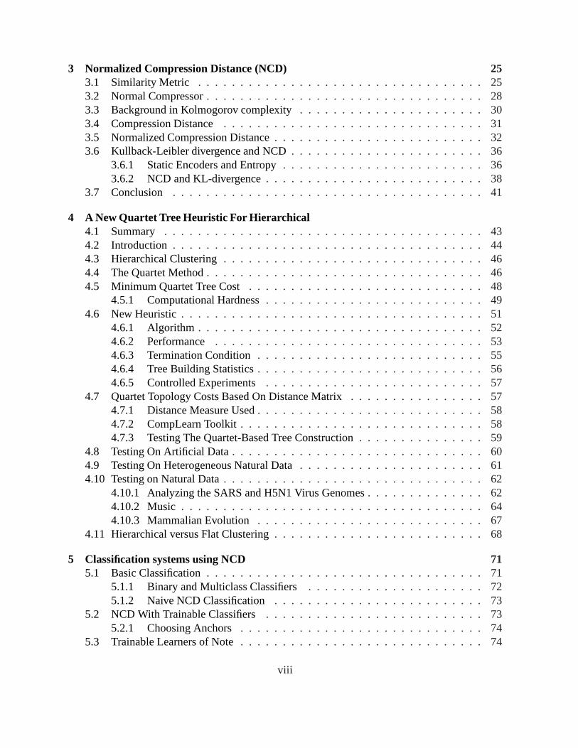
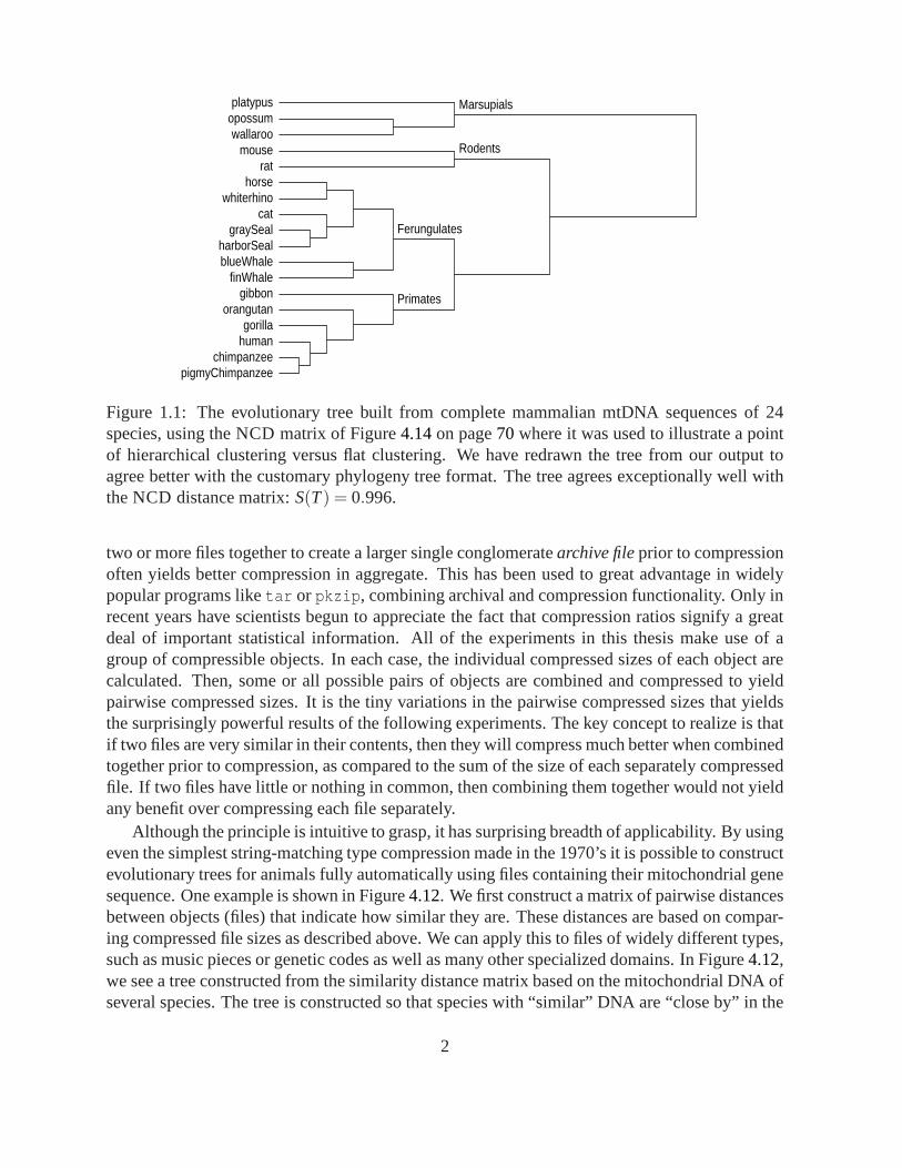
1.1 The evolutionary tree built from complete mammalian mtDNA sequences of 24species, using the NCD matrix of Figure 4.14 on page 70 where it was usedto illustrate a point of hierarchical clustering versus flatclustering. We haveredrawn the tree from our output to agree better with the customary phylogenytree format. The tree agrees exceptionally well with the NCDdistance matrix:S(T) = 0.996. . . . . . . . . . . . . . . . . . . . . . . . . . . . . . . . . . . . 2
1.2 Several people’s names, political parties, regions, and other Chinese names.. . . 4
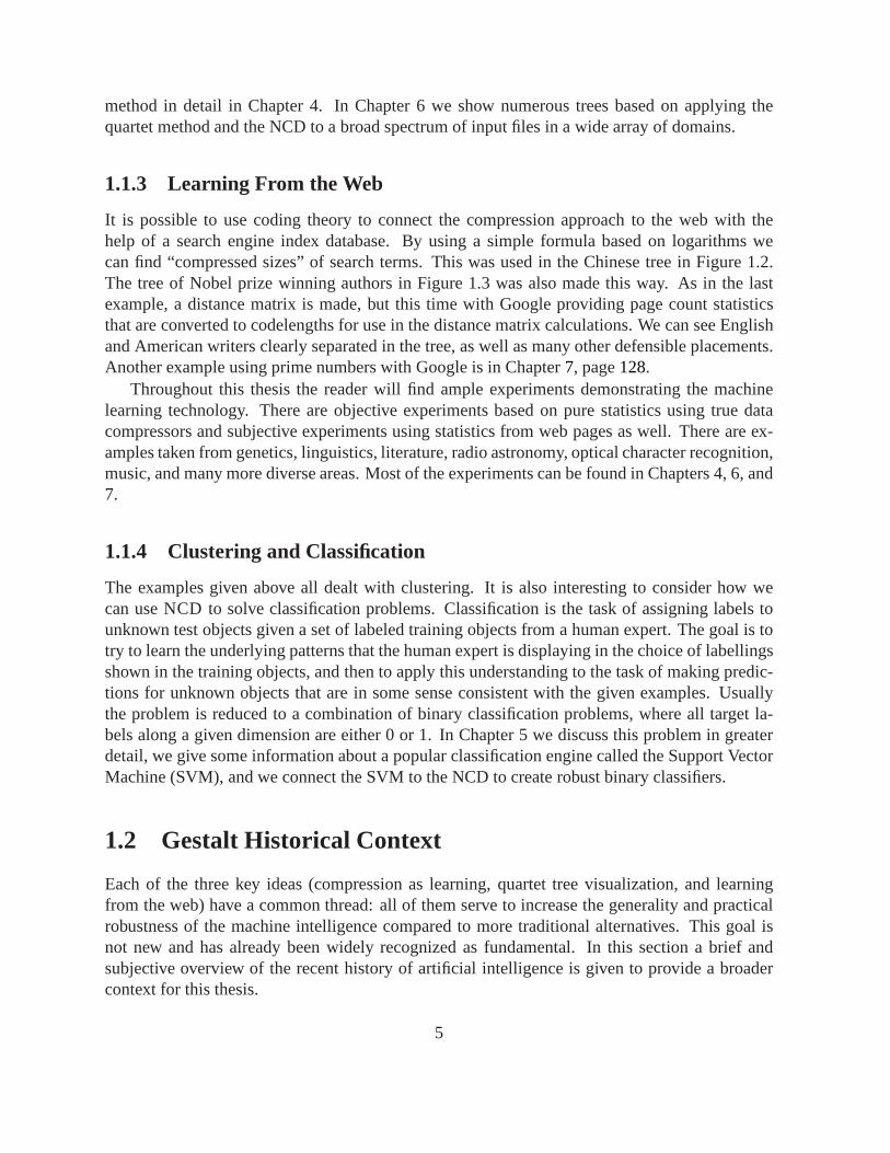
1.3 102 Nobel prize winning writers using CompLearn and NGD;S(T)=0.905630(part 3). . . . . . . . . . . . . . . . . . . . . . . . . . . . . . . . . . . . . . . . 6
3.1 A comparison of predicted and observed values forNCDR. . . . . . . . . . . . . 40
4.1 The three possible quartet topologies for the set of leaflabelsu,v,w,x. . . . . . . 47
4.2 An example tree consistent with quartet topologyuv|wx . . . . . . . . . . . . . . 48
4.3 Progress of a 60-item data set experiment over time.. . . . . . . . . . . . . . . . 54
4.4 Histogram of run-time number of trees examined before termination. . . . . . . . 56
4.5 Histogram comparing distributions ofk-mutations per run.. . . . . . . . . . . . 57
4.6 The randomly generated tree that our algorithm reconstructed.S(T) = 1. . . . . . 59
4.7 Classification of artificial files with repeated 1-kilobyte tags. Not all possibilitiesare included; for example, file “b” is missing.S(T) = 0.905. . . . . . . . . . . . 60
4.8 Classification of different file types. Tree agrees exceptionally well with NCDdistance matrix:S(T) = 0.984. . . . . . . . . . . . . . . . . . . . . . . . . . . . 61
xi
4.9 SARS virus among other virii. Legend: AvianAdeno1CELO.inp: Fowl ade-novirus 1; AvianIB1.inp: Avian infectious bronchitis virus (strain BeaudetteUS); AvianIB2.inp: Avian infectious bronchitis virus (strain Beaudette CK);BovineAdeno3.inp: Bovine adenovirus 3; DuckAdeno1.inp: Duck adenovirus 1;HumanAdeno40.inp: Human adenovirus type 40; HumanCorona1.inp: Humancoronavirus 229E; MeaslesMora.inp: Measles virus Moraten; MeaslesSch.inp:Measles virus strain Schwarz; MurineHep11.inp: Murine hepatitis virus strainML-11; MurineHep2.inp: Murine hepatitis virus strain 2; PRD1.inp: Enter-obacteria phage PRD1; RatSialCorona.inp: Rat sialodacryoadenitis coronavirus;SARS.inp: SARS TOR2v120403; SIRV1.inp: Sulfolobus SIRV-1; SIRV2.inp:Sulfolobus virus SIRV-2.S(T) = 0.988. . . . . . . . . . . . . . . . . . . . . . . 63
4.10 One hundred H5N1 (bird flu) sample genomes, S(T) = 0.980221. . . . . . . . . 654.11 Output for the 12-piece set.. . . . . . . . . . . . . . . . . . . . . . . . . . . . . 664.12 The evolutionary tree built from complete mammalian mtDNA sequences of 24
species, using the NCD matrix of Figure 4.14 on page 70 where it was usedto illustrate a point of hierarchical clustering versus flatclustering. We haveredrawn the tree from our output to agree better with the customary phylogenytree format. The tree agrees exceptionally well with the NCDdistance matrix:S(T) = 0.996. . . . . . . . . . . . . . . . . . . . . . . . . . . . . . . . . . . . 67
4.13 Multidimensional clustering of same NCD matrix (Figure 4.14) as used for Fig-ure 6.7. Kruskall’s stress-1 = 0.389.. . . . . . . . . . . . . . . . . . . . . . . . 68
4.14 Distance matrix of pairwise NCD. For display purpose, we have truncated theoriginal entries from 15 decimals to 3 decimals precision.. . . . . . . . . . . . . 70
6.1 Classification of different file types. Tree agrees exceptionally well with NCDdistance matrix:S(T) = 0.984. . . . . . . . . . . . . . . . . . . . . . . . . . . . 84
6.2 Output for the 36 pieces from 3 genres.. . . . . . . . . . . . . . . . . . . . . . 876.3 Output for the 12-piece set.. . . . . . . . . . . . . . . . . . . . . . . . . . . . . 886.4 Output for the 32-piece set.. . . . . . . . . . . . . . . . . . . . . . . . . . . . . 896.5 Output for the 60-piece set.. . . . . . . . . . . . . . . . . . . . . . . . . . . . . 906.6 Output for the set of 34 movements of symphonies.. . . . . . . . . . . . . . . . 916.7 The evolutionary tree built from complete mammalian mtDNA sequences of 24
species, using the NCD matrix of Figure 4.14 on page 70 where it was usedto illustrate a point of hierarchical clustering versus flatclustering. We haveredrawn the tree from our output to agree better with the customary phylogenytree format. The tree agrees exceptionally well with the NCDdistance matrix:S(T) = 0.996. . . . . . . . . . . . . . . . . . . . . . . . . . . . . . . . . . . . 95
6.8 Dendrogram of mitochondrial genomes of fungi using NCD.This represents thedistance matrix precisely withS(T) = 0.999. . . . . . . . . . . . . . . . . . . . 97
6.9 Dendrogram of mitochondrial genomes of fungi using block frequencies. Thisrepresents the distance matrix precisely withS(T) = 0.999. . . . . . . . . . . . . 97
6.10 Clustering of Native-American, Native-African, and Native-European languages.S(T) = 0.928. . . . . . . . . . . . . . . . . . . . . . . . . . . . . . . . . . . . . 98
xii
6.11 Clustering of Russian writers. Legend: I.S. Turgenev,1818–1883 [Father andSons, Rudin, On the Eve, A House of Gentlefolk]; F. Dostoyevsky 1821–1881[Crime and Punishment, The Gambler, The Idiot; Poor Folk]; L.N. Tolstoy 1828–1910 [Anna Karenina, The Cossacks, Youth, War and Piece]; N.V. Gogol 1809–1852 [Dead Souls, Taras Bulba, The Mysterious Portrait, Howthe Two IvansQuarrelled]; M. Bulgakov 1891–1940 [The Master and Margarita, The FatefullEggs, The Heart of a Dog].S(T) = 0.949. . . . . . . . . . . . . . . . . . . . . . 99
6.12 Clustering of Russian writers translated in English. The translator is given inbrackets after the titles of the texts. Legend: I.S. Turgenev, 1818–1883 [Fatherand Sons (R. Hare), Rudin (Garnett, C. Black), On the Eve (Garnett, C. Black),A House of Gentlefolk (Garnett, C. Black)]; F. Dostoyevsky 1821–1881 [Crimeand Punishment (Garnett, C. Black), The Gambler (C.J. Hogarth), The Idiot (E.Martin); Poor Folk (C.J. Hogarth)]; L.N. Tolstoy 1828–1910[Anna Karenina(Garnett, C. Black), The Cossacks (L. and M. Aylmer), Youth (C.J. Hogarth),War and Piece (L. and M. Aylmer)]; N.V. Gogol 1809–1852 [DeadSouls (C.J.Hogarth), Taras Bulba (≈ G. Tolstoy, 1860, B.C. Baskerville), The MysteriousPortrait + How the Two Ivans Quarrelled (≈ I.F. Hapgood]; M. Bulgakov 1891–1940 [The Master and Margarita (R. Pevear, L. Volokhonsky),The Fatefull Eggs(K. Gook-Horujy), The Heart of a Dog (M. Glenny)].S(T) = 0.953. . . . . . . 100
6.13 Images of handwritten digits used for OCR.. . . . . . . . . . . . . . . . . . . . 1006.14 Clustering of the OCR images.S(T) = 0.901. . . . . . . . . . . . . . . . . . . . 1016.15 16 observation intervals of GRS 1915+105 from four classes. The initial capital
letter indicates the class corresponding to Greek lower case letters in [5]. Theremaining letters and digits identify the particular observation interval in termsof finer features and identity. TheT-cluster is top left, theP-cluster is bottomleft, theG-cluster is to the right, and theD-cluster in the middle. This tree almostexactly represents the underlying NCD distance matrix:S(T) = 0.994. . . . . . 103
7.1 European Parliament members. . . . . . . . . . . . . . . . . . . . . . . . . . . 1067.2 Numbers versus log probability (pagecount / M) in a variety of languages and
formats. . . . . . . . . . . . . . . . . . . . . . . . . . . . . . . . . . . . . . . . 1217.3 Colors and numbers arranged into a tree using NGD .. . . . . . . . . . . . . . . 1237.4 Fifteen paintings tree by three different painters arranged into a tree hierarchical
clustering. In the experiment, only painting title names were used; the painterprefix shown in the diagram above was added afterwords as annotation to assistin interpretation. The painters and paintings used follow.Rembrandt van Rijn: Hendrickje slapend; Portrait of Maria Trip; Portrait of Johannes Wtenbogaert; The Stone Bridge ; The Prophetess Anna; Jan Steen : Leiden Baker ArendOostwaert ; Keyzerswaert ; Two Men Playing Backgammon ; Woman at herToilet ; Prince’s Day ; The Merry Family; Ferdinand Bol : Maria Rey ;Consul Titus Manlius Torquatus ; Swartenhont ; Venus and Adonis . . . . . . . . 124
7.5 Several people’s names, political parties, regions, and other Chinese names.. . . 1257.6 English Translation of Chinese Names. . . . . . . . . . . . . . . . . . . . . . . 126
xiii

7.7 Google-SVM learning of “emergencies.”. . . . . . . . . . . . . . . . . . . . . 1277.8 Google-SVM learning of primes.. . . . . . . . . . . . . . . . . . . . . . . . . . 1287.9 Google-SVM learning of “electrical” terms.. . . . . . . . . . . . . . . . . . . . 1297.10 Google-SVM learning of “religious” terms.. . . . . . . . . . . . . . . . . . . . 1307.11 Histogram of accuracies over 100 trials of WordNet experiment. . . . . . . . . . 1327.12 English-Spanish Translation Problem.. . . . . . . . . . . . . . . . . . . . . . . 1337.13 Translation Using NGD.. . . . . . . . . . . . . . . . . . . . . . . . . . . . . . 134
8.1 An excerpt of a 15th century manuscript ‘H’ from the collections of the HelsinkiUniversity Library, showing the beginning of the legend of St. Henry on the right:“Incipit legenda de sancto Henrico pontifice et martyre; lectio prima; Regnanteillustrissimo rege sancto Erico, in Suecia, uenerabilis pontifex beatus Henricus,de Anglia oriundus, ...”[47]. . . . . . . . . . . . . . . . . . . . . . . . . . . . . 138
8.2 An example tree obtained with the compression-based method. Changes arecircled and labeled with numbers 1–5. Costs of changes are listed in the box.Best reconstructions at interior nodes are written at the branching points.. . . . . 144
8.3 Best tree found. Most probable place of origin accordingto [47], see Table 8.5,indicated by color — Finland (blue): K,Ho,I,T,A,R,S,H,N,Fg; Vadstena (red):AJ,D,E,LT,MN,Y,JB,NR2,Li,F,G; Central Europe (yellow):JG,B; other (green).Some groups supported by earlier work are circled in red.. . . . . . . . . . . . . 146
8.4 Consensus tree. The numbers on the edges indicate the number of bootstrap treesout of 100 where the edge separates the two sets of variants. Large numberssuggest high confidence in the identified subgroup. Some groups supported byearlier work are circled in red.. . . . . . . . . . . . . . . . . . . . . . . . . . . 151
8.5 CompLearn tree showing many similarities with the tree in Fig. 8.3. . . . . . . . 152
9.1 Using thekitsch program in PHYLIP for comparison of H5N1 tree.. . . . . . . 1549.2 102 Nobel prize winning writers using CompLearn and NGD;S(T)=0.905630
(part 1). . . . . . . . . . . . . . . . . . . . . . . . . . . . . . . . . . . . . . . . 1569.3 102 Nobel prize winning writers using CompLearn and NGD;S(T)=0.905630
(part 2). . . . . . . . . . . . . . . . . . . . . . . . . . . . . . . . . . . . . . . . 1579.4 102 Nobel prize winning writers using CompLearn and NGD;S(T)=0.905630
(part 3). . . . . . . . . . . . . . . . . . . . . . . . . . . . . . . . . . . . . . . . 1589.5 102 Nobel prize winning writers using the PHYLIPkitsch. . . . . . . . . . . . . 159
xiv

List of Tables
6.1 The 60 classical pieces used (‘m’ indicates presence in the medium set, ‘s’ in thesmall and medium sets).. . . . . . . . . . . . . . . . . . . . . . . . . . . . . . 93
6.2 The 12 jazz pieces used.. . . . . . . . . . . . . . . . . . . . . . . . . . . . . . 946.3 The 12 rock pieces used.. . . . . . . . . . . . . . . . . . . . . . . . . . . . . . 94
xv


Acknowledgements
The author would like to thank first and foremost Dr. Paul Vitányi for his elaborate feedbackand tremendous technical contributions to this work. Next Ithank Dr. Peter Grünwald for amplefeedback. I also thank my colleagues John Tromp and Ronald deWolf. I thank my friendsDr. Kaihsu Tai and Ms. Anna Lissa Cruz for extensive feedbackand experimental inputs. Thisthesis is dedicated to my grandparents, Edwin and Dorothy, for their equanimity and support. Itis further dedicated in spirit to the memories of my mother, Theresa, for her compassion, and tomy father, Salvatore for his deep insight and foresight.
This work was supported in part by the Netherlands BSIK/BRICKS project, and by NWOproject 612.55.002, and by the IST Programme of the EuropeanCommunity, under the PASCALNetwork of Excellence, IST-2002-506778.
xvii

Papers on Which the Thesis is Based
Chapter 2 is introductory material, mostly based on M. Li andP.M.B. Vitányi. An Introduc-tion to Kolmogorov Complexity and Its Applications. Springer–Verlag, New York, secondedition, 1997.
Chapter 3 is based on R. Cilibrasi and P. Vitányi. Clusteringby compression.IEEE Transac-tions on Information Theory, 51(4):1523-1545, 2005, as well as M.Li, X. Chen, X. Li, B.Ma and P. Vitányi. The similarity metric.IEEE Trans. Information Theory, 50(12):3250–3264, 2004. Section3.6is based on unpublished work by R. Cilibrasi.
Chapter 4 is based on R. Cilibrasi and P.M.B. Vitányi. A new quartet tree heuristic for hierar-chical clustering, IEEE/ACM Trans. Comput. Biol. Bioinf.,Submitted. Presented at theEU-PASCAL Statistics and Optimization of Clustering Workshop, London, 2005,http://arxiv.org/abs/cs.DS/0606048
Chapter 5 is based on unpublished work by R. Cilibrasi.
Chapter 6 is based on
R. Cilibrasi and P. Vitányi. Clustering by compression.IEEE Transactions on InformationTheory, 51(4):1523-1545, 2005;
R. Cilibrasi, P.M.B. Vitányi, and R. de Wolf. Algorithmic clustering of music based onstring compression.Computer Music Journal, pages 49-67. A preliminary version ap-peared as
R. Cilibrasi, R. de Wolf, P. Vitányi, Algorithmic clustering of music,Proc IEEE 4th In-ternational Conference on Web Delivering of Music(WEDELMUSIC 2004), IEEE Comp.Soc. Press, 2004, 110-117.
This work was reported in among others: “Software to unzip identity of unknown com-posers,New Scientist, 12 April 2003, by Hazel Muir. “Software sorts tunes,”TechnologyResearch News, April 23/30, 2003, by Kimberly Patch; and “Classer musiques, langues,images, textes et genomes,”Pour La Science, 317(March 2004), 98–103, by Jean-PaulDelahaye , (Pour la Science = Edition francaise de ScientificAmerican).
xix
Chapter 7 is based on
R. Cilibrasi, P.M.B. Vitanyi, Automatic meaning discoveryusing Google,http://xxx.lanl.gov/abs/cs.CL/0412098 (2004); followed by conference versions
R. Cilibrasi and P.M.B. Vitányi, Automatic Extraction of Meaning from the Web,2006IEEE International Symposium on Information Theory (ISIT 2006), Seattle, 2006; and
R. Cilibrasi, P.M.B. Vitányi, Similarity of objects and themeaning of words,Proc. 3rdConf. Theory and Applications of Models of Computation (TAMC), 15-20 May, 2006,Beijing, China. Lecture Notes in Computer Science, Vol. 3959, Jin-Yi Cai, S. BarryCooper, and Angsheng Li (Eds.), 2006; to the journal version
R. Cilibrasi and P.M.B. Vitányi. The Google similarity distance,IEEE Transactions onKnowledge and Data Engineering, To appear.
The supporting experimental data for the binary classification experimental comparisonwith WordNet can be found athttp://www.cwi.nl/ cilibrar/googlepaper/appendix.eps
This work was reported in, among others, “A search for meaning,” New Scientist, 29 Jan-uary 2005, p.21, by Duncan Graham-Rowe; on the Web in “Deriving semantics meaningfrom Google results,”Slashdot— News for nerds, Stuff that matters, Discussion in theScience section, 29 January, 2005.
Chapter 8 is based on T. Roos, T. Heikkila, R. Cilibrasi, and P. Myllymäki. Compression-basedstemmatology: A study of the legend of St. Henry of Finland, 2005. HIIT technical report,http://cosco.hiit.fi/Articles/hiit-2005-3.eps
Chapter 9 is based on unpublished work by R. Cilibrasi.
Chapter 10 describes the CompLearn system, a general software tool to apply the ideas in thisThesis, written by R. Cilibrasi, and explains the reasoningbehind it; seehttp://complearn.org/ for more information.
xx

Chapter 1
Introduction
But certainly for the present age, which prefers the sign to the thing signified, thecopy to the original, representation to reality, the appearance to the essence... illusiononly is sacred, truth profane. Nay, sacredness is held to be enhanced in proportionas truth decreases and illusion increases, so that the highest degree of illusion comesto be the highest degree of sacredness. –Feuerbach, Prefaceto the second edition ofThe Essence of Christianity
1.1 Overview of this thesis
This thesis concerns a remarkable new scientific development that advances the state of the artin the field of data mining, or searching for previously unknown but meaningful patterns in fullyor semi-automatic ways. A substantial amount of mathematical theory is presented as well asvery many (though not yet enough) experiments. The results serve to test, verify, and demon-strate the power of this new technology. The core ideas of this thesis relate substantially to datacompression programs. For more than 30 years, data compression software has been developedand significantly improved with better models for almost every type of file. Until recently, themain driving interests in such technology were to economizeon disk storage or network datatransmission costs. A new way of looking at data compressorsand machine learning allows usto use compression programs for a wide variety of problems.
In this thesis a few themes are important. The first is the use of data compressors in newways. The second is a new tree visualization technique. And the third is an information-theoreticconnection of a web search engine to the data mining system. Let us examine each of these inturn.
1.1.1 Data Compression as Learning
The first theme concerns the statistical significance of compressed file sizes. Most computerusers realize that there are freely available programs thatcan compress text files to about onequarter their original size. The less well known aspect of data compression is that combining
1
platypusopossumwallaroo
Marsupials
mouserat
Rodents
horsewhiterhino
catgraySeal
harborSealblueWhale
finWhale
Ferungulates
gibbonorangutan
gorillahuman
chimpanzeepigmyChimpanzee
Primates
Figure 1.1: The evolutionary tree built from complete mammalian mtDNA sequences of 24species, using the NCD matrix of Figure4.14on page70 where it was used to illustrate a pointof hierarchical clustering versus flat clustering. We have redrawn the tree from our output toagree better with the customary phylogeny tree format. The tree agrees exceptionally well withthe NCD distance matrix:S(T) = 0.996.
two or more files together to create a larger single conglomeratearchive fileprior to compressionoften yields better compression in aggregate. This has beenused to great advantage in widelypopular programs liketar or pkzip, combining archival and compression functionality. Only inrecent years have scientists begun to appreciate the fact that compression ratios signify a greatdeal of important statistical information. All of the experiments in this thesis make use of agroup of compressible objects. In each case, the individualcompressed sizes of each object arecalculated. Then, some or all possible pairs of objects are combined and compressed to yieldpairwise compressed sizes. It is the tiny variations in the pairwise compressed sizes that yieldsthe surprisingly powerful results of the following experiments. The key concept to realize is thatif two files are very similar in their contents, then they willcompress much better when combinedtogether prior to compression, as compared to the sum of the size of each separately compressedfile. If two files have little or nothing in common, then combining them together would not yieldany benefit over compressing each file separately.
Although the principle is intuitive to grasp, it has surprising breadth of applicability. By usingeven the simplest string-matching type compression made inthe 1970’s it is possible to constructevolutionary trees for animals fully automatically using files containing their mitochondrial genesequence. One example is shown in Figure4.12. We first construct a matrix of pairwise distancesbetween objects (files) that indicate how similar they are. These distances are based on compar-ing compressed file sizes as described above. We can apply this to files of widely different types,such as music pieces or genetic codes as well as many other specialized domains. In Figure4.12,we see a tree constructed from the similarity distance matrix based on the mitochondrial DNA ofseveral species. The tree is constructed so that species with “similar” DNA are “close by” in the
2
tree. In this way we may lend support to certain evolutionarytheories.Although simple compressors work, it is also easy to use the most advanced modern com-
pressors with the theory presented in this thesis; these results can often be more accurate thansimpler compressors in a variety of particular circumstances or domains. The main advantage ofthis approach is its robustness in the face of strange or erroneous data. Another key advantage isthe simplicity and ease of use. This comes from the generality of the method: it works in a va-riety of different application domains and when using general-purpose compressors it becomesa general-purpose inference engine. Throughout this thesis there is a focus on coding theoryand data compression, both as a theoretical construct as well as practical approximations thereofthrough actual data compression programs in current use. There is a connection between a partic-ular code and a probability distribution and this simple theoretical foundation allows one to usedata compression programs of all types as statistical inference engines of remarkable robustnessand generality. In Chapter 3, we describe theNormalized Compression Distance(NCD), whichformalizes the ideas we have just described. We report on a plethora of experiments in Chapter 6showing applications in a variety of interesting problems in data mining using gene sequences,music, text corpora, and other inputs.
1.1.2 Visualization
Custom open source software has been written to provide powerful new visualization capabilities.TheCompLearnsoftware system (Chapter10) implements our theory and with it experiments oftwo types may be carried out: classification or clustering. Classification refers to the applicationof discrete labels to a set of objects based on a set of examples from a human expert. Clusteringrefers to arrangement of objects into groups without prior training or influence by a human expert.In this thesis we deal primarily with hierarchical or nestedclustering in which a group of objectsis arranged into a sort of binary tree. This clustering method is called thequartet methodandwill be discussed in detail later.
In a nutshell, the quartet method is a way to determine a best matching tree given some datathat is to be understood in a hierarchical cluster. It is called the quartet method because it is basedon the smallest unrooted binary tree, which happens to be twopairs of two nodes for a total offour nodes comprising the quartet. It adds up many such smallbinary trees together to evaluatea big tree and then adjusts the tree according to the results of the evaluation. After a time, abest fitting tree is declared and the interpretation of the experimental results is possible. Thecompression-based algorithms output a matrix of pairwise distances between objects. Becausesuch a matrix is hard to interpret, we try to extract some of its essential features using the quartetmethod. This results in a tree optimized so that similar objects with small distances are placednearby each other. The trees given in Figures 1.1, 1.2, and 1.3 (discussed below) have all beenconstructed using the quartet method.
The quartet tree search is non-deterministic. There are compelling theoretical reasons tosuppose that the general quartet tree search problem is intractable to solve exactly for every case.But the method used here tries instead to approximate a solution in a reasonable amount of time,sacrificing accuracy for speed. It also makes extensive use of random numbers, and so there issometimes variation in the results that the tree search produces. We describe the quartet tree
3

Figure 1.2: Several people’s names, political parties, regions, and other Chinese names.4
method in detail in Chapter 4. In Chapter 6 we show numerous trees based on applying thequartet method and the NCD to a broad spectrum of input files ina wide array of domains.
1.1.3 Learning From the Web
It is possible to use coding theory to connect the compression approach to the web with thehelp of a search engine index database. By using a simple formula based on logarithms wecan find “compressed sizes” of search terms. This was used in the Chinese tree in Figure 1.2.The tree of Nobel prize winning authors in Figure 1.3 was alsomade this way. As in the lastexample, a distance matrix is made, but this time with Googleproviding page count statisticsthat are converted to codelengths for use in the distance matrix calculations. We can see Englishand American writers clearly separated in the tree, as well as many other defensible placements.Another example using prime numbers with Google is in Chapter 7, page128.
Throughout this thesis the reader will find ample experiments demonstrating the machinelearning technology. There are objective experiments based on pure statistics using true datacompressors and subjective experiments using statistics from web pages as well. There are ex-amples taken from genetics, linguistics, literature, radio astronomy, optical character recognition,music, and many more diverse areas. Most of the experiments can be found in Chapters 4, 6, and7.
1.1.4 Clustering and Classification
The examples given above all dealt with clustering. It is also interesting to consider how wecan use NCD to solve classification problems. Classificationis the task of assigning labels tounknown test objects given a set of labeled training objectsfrom a human expert. The goal is totry to learn the underlying patterns that the human expert isdisplaying in the choice of labellingsshown in the training objects, and then to apply this understanding to the task of making predic-tions for unknown objects that are in some sense consistent with the given examples. Usuallythe problem is reduced to a combination of binary classification problems, where all target la-bels along a given dimension are either 0 or 1. In Chapter 5 we discuss this problem in greaterdetail, we give some information about a popular classification engine called the Support VectorMachine (SVM), and we connect the SVM to the NCD to create robust binary classifiers.
1.2 Gestalt Historical Context
Each of the three key ideas (compression as learning, quartet tree visualization, and learningfrom the web) have a common thread: all of them serve to increase the generality and practicalrobustness of the machine intelligence compared to more traditional alternatives. This goal isnot new and has already been widely recognized as fundamental. In this section a brief andsubjective overview of the recent history of artificial intelligence is given to provide a broadercontext for this thesis.
5
Figure 1.3: 102 Nobel prize winning writers using CompLearnand NGD; S(T)=0.905630 (part3).
6
In the beginning, there was the idea of artificial intelligence. As circuit miniaturization tookoff in the 1970’s, people’s imaginations soared with ideas of a new sort of machine with virtuallyunlimited potential: a (usually humanoid) metal automatonwith the capacity to perform intelli-gent work and yet ask not one question out of the ordinary. A sort of ultra-servant, made able toreason as well as man in most respects, yet somehow reasoningin a sort of rarefied form wherebythe more unpredictable sides of human nature are factored out. One of the first big hurdles cameas people tried to define just what intelligence was, or how one might codify knowledge in themost general sense into digital form. As Levesque and Brachman famously observed [73], rea-soning and representation are hopelessly intertwined, andjust what intelligence is depends verymuch on just who is doing the talking.
Immediately upon settling on the question of intelligence one almost automatically mustgrapple with the concept of language. Consciousness and intelligence is experienced only in-ternally, yet the objects to which it applies are most often external to the self. Thus there isat once the question of communication and experience and this straight-away ends any hope ofperfect answers. Most theories on language are not theoriesin the formal sense [14]. A notableearly exception is Quine’s famous observation that language translation is necessarily a diceysubject: for although you might collect very many pieces of evidence suggesting that a wordmeans “X” or “Y”, you can never collect a piece of evidence that ultimately confirms that yourunderstanding of the word is “correct” in any absolute sense. In a logical sense, we can never besure that the meaning of a word is as it was meant, for to explain any word we must use otherwords, and these words themselves have only other words to describe them, in an interminableweb of ontological disarray. Kantian empiricism leads us topragmatically admit we have onlythe basis of our own internal experience to ground our understanding at the most basic level, andthe mysterious results of the reasoning mind, whatever thatmight be.
It is without a doubt the case that humans throughout the world develop verbal and usuallywritten language quite naturally. Recent theories by Smale[38] have provided some theoreticalsupport for empirical models of language evolution despitethe formal impossibility of absolutecertainty. Just the same it leaves us with a very difficult question: how do we make bits think?
Some twenty years later, progress has been bursty. We have managed to create some amaz-ingly elegant search and optimization techniques including simplex optimization, tree search,curve-fitting, and modern variants such as neural networks or support vector machines. We havebuilt computers that can beat any human in chess, but we cannot yet find a computer smartenough to walk to the grocery store to buy a loaf of bread. There is clearly a problem of overspe-cialization in the types of successes we have so far enjoyed in artificial intelligence. This thesisexplores my experience in charting this new landscape of concepts via a combination of prag-matic and principled techniques. It is only with the recent explosion in internet use and internetwriting that we can now begin to seriously tackle these problems so fundamental to the originaldream of artificial intelligence.
In recent years, we have begun to make headway in defining and implementing universal pre-diction, arguably the most important part of artificial intelligence. Most notable is Solomonoffprediction [105], and the more practical analogs by Ryabko and Astola [98] using data compres-sion.
In classical statistical settings, we typically make some observations of a natural (or at the
7
very least, measurable) phenomenon. Next, we use our intuition to “guess” which mathematicalmodel might best apply. This process works well for those cases where the guesser has a goodmodel for the phenomenon under consideration. This allows for at least two distinct modes offreedom: both in the choice of models, and also in the choice of criteria supporting “goodness”.
In the past the uneasy compromise has been to focus attentionfirstly on those problemswhich are most amenable to exact solution, to advance the foundation of exact and fundamentalscience. The next stage of growth was the advent of machine-assisted exact sciences, such as thenow-famous four-color proof that required input (by hand!)of 1476 different graphs for com-puter verification (by a complicated program) that all were colorable before deductive extensionto the most general case in the plane [2]. After that came the beginning of modern machinelearning, based on earlier ideas of curve fitting and least-squares regression. Neural networks,and later support vector machines, gave us convenient learning frameworks in the context of con-tinuous functions. Given enough training examples, the theory assured us, the neural networkwould eventually find the right combination of weightings and multiplicative factors that wouldmiraculously, and perhaps a bit circularly, reflect the underlying meaning that the examples weremeant to teach. Just like spectral analysis that came before, each of these areas yielded a wholenew broad class of solutions, but were essentially hit or miss in their effectiveness in each do-main for reasons that remain poorly understood. The focus ofmy research has been on the useof data compression programs for generalized inference. Itturns out that this modus operandiis surprisingly general in its useful application and yields oftentimes the most expedient resultsas compared to other more predetermined methods. It is often“one size fits all well enough”and this yields unexpected fruits. From the outset, it must be understood that the approach hereis decidedly different than more classical ones, in that we avoid in most ways an exact state-ment of the problem at hand, instead deferring this until very near the end of the discussion, sothat we might better appreciate what can be understood aboutall problems with a minimum ofassumptions.
At this point a quote from Goldstein and Gigerenzer [43] is appropriate:
What are heuristics? The Gestalt psychologists Karl Duncker and Wolfgang Koehlerpreserved the original Greek definition of “serving to find out or discover” whenthey used the term to describe strategies such as “looking around” and “inspectingthe problem” (e.g., Duncker, 1935/1945).
For Duncker, Koehler, and a handful of later thinkers, including Herbert Simon (e.g.,1955), heuristics are strategies that guide information search and modify problemrepresentations to facilitate solutions. From its introduction into English in the early1800s up until about 1970, the term heuristics has been used to refer to useful and in-dispensable cognitive processes for solving problems thatcannot be handled by logicand probability theory (e.g., Polya, 1954; Groner, Groner,& Bischof, 1983). In thepast 30 years, however, the definition of heuristics has changed almost to the point ofinversion. In research on reasoning, judgment, and decision making, heuristics havecome to denote strategies that prevent one from finding out ordiscovering correctanswers to problems that are assumed to be in the domain of probability theory. Inthis view, heuristics are poor substitutes for computations that are too demanding for
8
ordinary minds to carry out. Heuristics have even become associated with inevitablecognitive illusions and irrationality.
This author sides with Goldstein and Gigerenzer in the view that sometimes “less is more”;the very fact that things are unknown to the naive observer can sometimes work to his advantage.The recognition heuristic is an important, reliable, and conservative general strategy for inductiveinference. In a similar vein, the NCD based techniques shownin this thesis provide a generalframework for inductive inference that is robust against a wide variety of circumstances.
1.3 Contents of this Thesis
In this chapter a summary is provided for the remainder of thethesis as well as some historicalcontext. In Chapter 2, an introduction to the technical details and terminology surrounding themethods is given. In chapter 3 we introduce the Normalized Compression Distance (NCD), thecore mathematical formula that makes all of these experiments possible, and we establish con-nections between NCD and other well-known mathematical formulas. In Chapter 4 a tree searchsystem is explained based on groups of four objects at a time,the so-calledquartet method. InChapter 5 we combine NCD with other machine learning techniques such as Support VectorMachines. In Chapter 6, we provide a wealth of examples of this technology in action. Allexperiments in this thesis were done using the CompLearn Toolkit, an open-source general pur-pose data mining toolkit available for download from thehttp://complearn.org/ website. InChapter 7, we show how to connect the internet to NCD using theGoogle search engine, thusproviding the advanced sort of subjective analysis as shownin Figure 1.2. In Chapter 8 we usethese techniques and others to trace the evolution of the legend of Saint Henry. In Chapter 9 wecompare CompLearn against another older tree search software system called PHYLIP. Chap-ter 10 gives a snapshot of the online documentation for the CompLearn system. After this, aDutch language summary is provided as well as a bibliography, index, and list of papers byR. Cilibrasi.
9

Chapter 2
Technical Introduction
The spectacle is the existing order’s uninterrupted discourse about itself, its lauda-tory monologue. It is the self-portrait of power in the epochof its totalitarian man-agement of the conditions of existence. The fetishistic, purely objective appear-ance of spectacular relations conceals the fact that they are relations among men andclasses: a second nature with its fatal laws seems to dominate our environment. Butthe spectacle is not the necessary product of technical development seen as a naturaldevelopment. The society of the spectacle is on the contrarythe form which choosesits own technical content. –Guy Debord,Society of the Spectacle
This chapter will give an informal introduction to relevantbackground material, familiarizingthe reader with notation and basic concepts but omitting proofs. We discuss strings, languages,codes, Turing Machines and Kolmogorov complexity. This material will be extensively used inthe chapters to come. For a more thorough and detailed treatment of all the material including atremendous number of innovative proofs see [79]. It is assumed that the reader has a basic famil-iarity with algebra and probability theory as well as some rudimentary knowledge of classicalinformation theory. We first introduce the notions offinite, infinite andstring of characters. Wego on to discuss basic coding theory. Next we introduce the idea of Turing Machines. Finally, inthe last part of the chapter, we introduce Kolmogorov Complexity.
2.1 Finite and Infinite
In the domain of mathematical objects discussed in this thesis, there are two broad categories:finite and infinite.Finite objects are those whose extent is bounded.Infiniteobjects are those thatare “larger” than any given precise bound. For example, if weperform 100 flips of a fair coin insequence and retain the results in order, the full record will be easily written upon a single sheetof A4 size paper, or even a business card. Thus, the sequence is finite. But if we instead talkabout the list of all prime numbers greater than 5, then the sequence written literally is infinitein extent. There are far too many to write on any given size of paper no matter how big. It ispossible, however, to write acomputer programthat could, in principle, generate every prime
11
number, no matter how large, eventually, given unlimited time and memory. It is important torealize that some objects are infinite in their totality, butcan be finite in a potential effectivesense by the fact that every finite but a priori unbounded partof them can be obtained from afinite computer program. There will be more to say on these matters later in Section2.5.
2.2 Strings and Languages
A bit, or binary digit, is just a single piece of information representing a choice between one oftwo alternatives, either 0 or 1.
A character is a symbol representing an atomic unit of written language that cannot be mean-ingfully subdivided into smaller parts. An alphabet is a setof symbols used in writing a givenlanguage. A language (in the formal sense) is a set of permissiblestringsmade from a givenalphabet. Astring is an ordered list (normally written sequentially) of 0 or more symbols drawnfrom a common alphabet. For a given alphabet, different languages deem different strings per-missible. In English, 26 letters are used, but also the spaceand some punctuation should beincluded for convenience, thus increasing the size of the alphabet. In computer files, the under-lying base is 256 because there are 256 different states possible in each indivisible atomic unitof storage space, thebyte. A byte is equivalent to 8 bits, so the 256-symbol alphabet iscentral toreal computers. For theoretical purposes however, we can dispense with the complexities of largealphabets by realizing that we can encode large alphabets into small ones; indeed, this is how abyte can be encoded as 8 bits. A bit is a symbol from a 2-symbol,or binary, alphabet. In thisthesis, there is not usually any need for an alphabet of more than two characters, so the notationalconvention is to restrict attention to the binary alphabet in the absence of countervailing remarks.Usually we encode numbers as a sequence of characters in a fixed radix format at the most basiclevel, and the space required to encode a number in this format can be calculated with the helpof the logarithm function. The logarithm function is alwaysused to determine a coding lengthfor a given number to be encoded, given a probability or integer range. Similarly, it is safe forthe reader to assume that all log’s are taken base 2 so that we may interpret the results in bits.
We write Σ to represent the alphabet used. We usually work with the binary alphabet, soin that caseΣ = 0,1. We writeΣ∗ to represent the space of all possible strings including theempty string. This notation may be a bit unfamiliar at first, but is very convenient and is relatedto the well-known concept ofregular expressions. Regular expressions are a concise way ofrepresenting formal languages as sets of strings over an alphabet. The curly braces represent aset(to be used as the alphabet in this case) and the∗ symbol refers to theclosureof the set; Byclosurewe mean that the symbol may be repeated 0, 1, 2, 3, 5, or any number of times. Bydefinition,0,1∗ =
S
n≥00,1n. It is important to realize that successive symbols need notbethe same, but could be. Here we can see that the number of possible binary strings is infinite, yetany individual string in this class must itself be finite. Fora stringx, we write|x| to represent thelength, measured in symbols, of that string.
12
2.3 The Many Facets of Strings
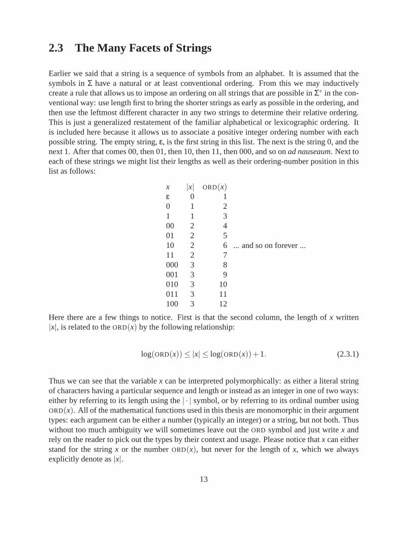
Earlier we said that a string is a sequence of symbols from an alphabet. It is assumed that thesymbols inΣ have a natural or at least conventional ordering. From this we may inductivelycreate a rule that allows us to impose an ordering on all strings that are possible inΣ∗ in the con-ventional way: use length first to bring the shorter strings as early as possible in the ordering, andthen use the leftmost different character in any two stringsto determine their relative ordering.This is just a generalized restatement of the familiar alphabetical or lexicographic ordering. Itis included here because it allows us to associate a positiveinteger ordering number with eachpossible string. The empty string,ε, is the first string in this list. The next is the string 0, and thenext 1. After that comes 00, then 01, then 10, then 11, then 000, and so onad nauseaum. Next toeach of these strings we might list their lengths as well as their ordering-number position in thislist as follows:
x |x| ORD(x)ε 0 10 1 21 1 300 2 401 2 510 2 611 2 7000 3 8001 3 9010 3 10011 3 11100 3 12
... and so on forever ...
Here there are a few things to notice. First is that the secondcolumn, the length ofx written|x|, is related to theORD(x) by the following relationship:
log(ORD(x))≤ |x| ≤ log(ORD(x))+1. (2.3.1)
Thus we can see that the variablex can be interpreted polymorphically: as either a literal stringof characters having a particular sequence and length or instead as an integer in one of two ways:either by referring to its length using the| · | symbol, or by referring to its ordinal number usingORD(x). All of the mathematical functions used in this thesis are monomorphic in their argumenttypes: each argument can be either a number (typically an integer) or a string, but not both. Thuswithout too much ambiguity we will sometimes leave out theORD symbol and just writex andrely on the reader to pick out the types by their context and usage. Please notice thatx can eitherstand for the stringx or the numberORD(x), but never for the length ofx, which we alwaysexplicitly denote as|x|.
13

2.4 Prefix Codes
A binary stringy is a proper prefixof a binary stringx if we can writex = yz for z 6= ε. A setx,y, . . . ⊆ 0,1∗ is prefix-freeif no element is a proper prefix of any other. A prefix-free setcan be used to define aprefix code. Formally, a prefix code is defined by adecoding function D,which is a function from a prefix free set to some arbitrary setX . The elements of the prefix freeset are calledcode words. The elements ofX are calledsource words. If the inverseD−1 of Dexists, we call it theencoding function. An example of a prefix code, that is used later, encodesa source wordx = x1x2 . . .xn by the code word
x = 1n0x.
HereX = 0,1∗, D−1(x) = x = 1n0x. This prefix-free code is calledself-delimiting, becausethere is a fixed computer program associated with this code that can determine where the codeword x ends by reading it from left to right without backing up. Thisway a composite codemessage can be parsed in its constituent code words in one pass by a computer program.1
In other words, a prefix code is a code in which no codeword is a prefix of another codeword.Prefix codes are very easy to decode because codeword boundaries are directly encoded alongwith each datum that is encoded. To introduce these, let us consider how we may combine anytwo strings together in a way that they could be later separated without recourse to guessing. Inthe case of arbitrary binary stringsx,y, we cannot be assured of this prefix condition:x mightbe 0 whiley was 00 and then there would be no way to tell the original contents ofx or y given,say, justxy. Therefore let us concentrate on just thex alone and think about how we mightaugment the natural literal encoding to allow for prefix disambiguation. In real languages oncomputers, we are blessed with whitespace and commas, both of which are used liberally for thepurpose of separating one number from the next in normal output formats. In a binary alphabetour options are somewhat more limited but still not too bad. The simplest solution would be toadd in commas and spaces to the alphabet, thus increasing thealphabet size to 4 and the codingsize to 2 bits, doubling the length of all encoded strings. This is a needlessly heavy price to payfor the privilege of prefix encoding, as we will soon see. But first let us reconsider another way todo it in a bit more than double space: suppose we prefacex with a sequence of|x| 0’s, followedby a 1, followed by the literal stringx. This then takes one bit more than twice the space forxand is even worse than the original scheme with commas and spaces added to the alphabet. Thisis just the scheme discussed in the beginning of the section.But this scheme has ample roomfor improvement: suppose now we adjust it so that instead of outputting all those 0’s at first inunary, we instead just output a number of zeros equal to
⌈log(|x|)⌉,then a 1, then the binary number|x| (which satisfies|x| ≤ ⌈logx⌉+ 1, see Eq. (2.3.1)), thenxliterally. Here,⌈·⌉ indicates the ceiling operation that returns the smallest integer not less than
1This desirable property holds for every prefix-free encoding of a finite set of source words, but not for everyprefix-free encoding of an infinite set of source words. For a single finite computer program to be able to parse acode message the encoding needs to have a certain uniformityproperty like thex code.
14

its argument. This, then, would take a number of bits about
2⌈log logx⌉+ ⌈logx⌉+1,
which exceeds⌈logx⌉, the number of bits needed to encodex literally, only by a logarithmicamount. If this is still too many bits then the pattern can be repeated, encoding the first set of 0’sone level higher using the system to get
2⌈logloglogx⌉+ ⌈log logx⌉+ ⌈logx⌉+1.
Indeed, we can “dial up” as many logarithms as are necessary to create a suitably slowly-growingcomposition of however many log’s are deemed appropriate. This is sufficiently efficient for allpurposes in this thesis and provides a general framework forconverting arbitrary data into prefix-free data. It further allows us to compose any number of strings or numbers for any purposewithout restraint, and allows us to make precise the difficult concept ofK(x,y), as we shall seein Section2.6.4.
2.4.1 Prefix Codes and the Kraft Inequality
Let X be the set of natural numbers and consider the straightforward non-prefix binary represen-tation with theith binary string in the length-increasing lexicographicalorder corresponding tothe numberi. There are two elements ofX with a description of length 1, four with a descriptionof length 2 and so on. However, there are less binary prefix code words of each length: ifx isa prefix code word then noy = xz with z 6= ε is a prefix code word. Asymptotically there areless prefix code words of lengthn than the 2n source words of lengthn. Clearly this observationholds for arbitrary prefix codes. Quantification of this intuition for countableX and arbitraryprefix-codes leads to a precise constraint on the number of code-words of given lengths. Thisimportant relation is known as theKraft Inequalityand is due to L.G. Kraft [60].
2.4.1.LEMMA . Let l1, l2, . . . be a finite or infinite sequence of natural numbers. There is a prefixcode with this sequence as lengths of its binary code words iff
∑n
2−ln ≤ 1. (2.4.1)
2.4.2 Uniquely Decodable Codes
We want to code elements of some setX in a way that they can be uniquely reconstructed from theencoding. Such codes are calleduniquely decodable. Every prefix-code is a uniquely decodablecode. On the other hand, not every uniquely decodable code satisfies the prefix condition. Prefix-codes are distinguished from other uniquely decodable codes by the property that the end ofa code word is always recognizable as such. This means that decoding can be accomplishedwithout the delay of observing subsequent code words, whichis why prefix-codes are also calledinstantaneous codes. There is good reason for our emphasis on prefix-codes. Namely, it turnsout that Lemma2.4.1 stays valid if we replace “prefix-code” by “uniquely decodable code.”
15

This important fact means that every uniquely decodable code can be replaced by a prefix-codewithout changing the set of code-word lengths. In this thesis, the only aspect of actual encodingsthat interests us is their length, because this reflects the underlying probabilities in an associatedmodel. There is no loss of generality in restricting furtherdiscussion to prefix codes because ofthis property.
2.4.3 Probability Distributions and Complete Prefix Codes
A uniquely decodable code iscompleteif the addition of any new code word to its code wordset results in a non-uniquely decodable code. It is easy to see that a code is complete iff equal-ity holds in the associated Kraft Inequality. Letl1, l2, . . . be the code words of some completeuniquely decodable code. Let us defineqx = 2−lx. By definition of completeness, we have∑xqx = 1. Thus, theqx can be thought of asprobability mass functionscorresponding to someprobability distributionQ for a random variableX. We sayQ is the distributioncorrespondingtol1, l2, . . .. In this way, each complete uniquely decodable code is mapped to a unique probabilitydistribution. Of course, this is nothing more than a formal correspondence: we may choose toencode outcomes ofX using a code corresponding to a distributionq, whereas the outcomes areactually distributed according to somep 6= q. But, as we argue below, ifX is distributed accord-ing to p, then the code to whichp corresponds is, in an average sense, the code that achievesoptimal compression ofX. In particular, every probability mass functionp is related to a prefixcode, theShannon-Fano code, such that the expected number of bits per transmitted code wordis as low as is possible for any prefix code, assuming that a random sourceX generates the sourcewordsx according toP(X = x) = p(x). The Shannon-Fano prefix code encodes a source wordx by a code word of lengthlx = ⌈log1/p(x)⌉, so that the expected transmitted code word lengthequals∑x p(x) log1/p(x) = H(X), the entropy of the sourceX, up to one bit. This is optimal byShannon’s “noiseless coding” theorem [102]. This is further explained in Section2.7.
2.5 Turing Machines
This section mainly serves as a preparation for the next section, in which we introduce the funda-mental concept ofKolmogorov complexity. Roughly speaking, the Kolmogorov complexity of astring is the shortest computer program that computes the string, i.e. that prints it, and then halts.The definition depends on the specific computer programming language that is used. To make thedefinition more precise, we should base it on programs written for universal Turing machines,which are an abstract mathematical representation of a general-purpose computer equipped witha general-purpose oruniversalcomputer programming language.
Universal Computer Programming Languages: Most popular computer programming lan-guages such as C, Lisp, Java and Ruby, areuniversal. Roughly speaking, this means that theymust be powerful enough to emulate any other computer programming language: every universalcomputer programming language can be used to write a compiler for any other programming lan-guage, including any other universal programming language. Indeed, this has been done already
16

a thousand times over with the GNU (Gnu’s Not Unix) C compiler, perhaps the most successfulopen-source computer program in the world. In this case, although there are many different as-sembly languages in use on different CPU architectures, allof them are able to run C programs.So we can always package any C program along with the GNU C compiler which itself is notmore than 100 megabytes in order to run a C program anywhere.
Turing Machines: TheTuring machineis an abstract mathematical representation of the ideaof a computer. It generalizes and simplifies all the many specific types of deterministic comput-ing machines into one regularized form. A Turing machine is defined by a set of rules whichdescribe its behavior. It receives as its input a string of symbols, wich may be thought OF as a“program”, and it outputs the result of running that program, which amounts to transforming theinput using the given set of rules. Just as there are universal computer languages, there are alsouniversal Turing machines. We say a Turing Machine is universal if it can simulate any otherTuring Machine. When such a universal Turing machine receives as input a pair〈x,y〉, wherexis a formal specification of another Turing machineTx, it outputs the same result as one wouldget if one would input the stringy to the Turing machineTx. Just as any universal programminglanguage can be used to emulate any other one, any universal Turing machine can be used toemulate any other one. It may help intuition to imagine any familiar universal computer pro-gramming language as a definition of a universal Turing machine, and the runtime and hardwareneeded to execute it as a sort of real-world Turing machine itself. It is necessary to remove re-source constraints (on memory size and input/output interface, for example) in order for theseconcepts to be thoroughly equivalent theoretically.
Turing machines, formally: A Turing machine consists of two parts: a finite control and atape. The finite control is the memory (or current state) of the machine. It always containsa single symbol from a finite setQ of possible states. The tape initially contains the programwhich the Turing machine must execute. The tape contains symbols from the trinary alphabetA = 0,1,B. Initially, the entire tape contains theB (blank) symbol except for the place wherethe program is stored. The program is a finite sequence of bits. The finite control also is alwayspositioned above a particular symbol on the tape and may moveleft or right one step. At first, thetape head is positioned at the first nonblank symbol on the tape. As part of the formal definitionof a Turing machine, we must indicate which symbol fromQ is to be the starting state of themachine. At every time step the Turing machine does a simple sort of calculation by consultinga list of rules that define its behavior. The rules may be understood to be a function taking twoarguments (the current state and the symbol under the reading head) and returning a Cartesianpair: the action to execute this timestep and the next state to enter. This is to say that the two inputarguments are a current state (symbol fromQ) of the finite control and a letter from the alphabetA. The two outputs are a new state (also taken fromQ) and anaction symbol taken fromS.The set of possible actions isS= 0,1,B,L,R. The 0, 1, andB symbols refer to writing thatvalue below the tape head. TheL andR symbols refer to moving left or right, respectively. Thisfunction defines the behavior of the Turing machine at each step, allowing it to perform simpleactions and run a program on a tape just like a real computer but in a very mathematically simple
17
way. It turns out that we can choose a particular set of state-transition rules such that the Turingmachine becomesuniversalin the sense described above. This simulation is plausible given amoment of reflection on how a Turing Machine is mechanically defined as a sequence of rulesgoverning state transitions etc. The endpoint in this line of reasoning is that a universal TuringMachine can run a sort of Turing Machine simulation system and thereby compute identicalresults as any other Turing Machine.
Notation: We typically use the Greek letterΦ to represent a Turing machineT as a partiallydefined function. When the Turing machineT is not clear from the context, we writeΦT . Thefunction is supposed to take as input a program encoded as a finite binary string and outputsthe results of running that program. Sometimes it is convenient to define the function as takingintegers instead of strings; this is easy enough to do when weremember that each integer is iden-tified with a given finite binary string given the natural lexicographic ordering of finite strings,as in Section2.3 The functionΦ need only be partially defined; for some input strings it is notdefined because some programs do not produce a finite string asoutput, such as infinite loopingprograms. We say thatΦ is defined only for those programs that halt and therefore produce adefinite output. We introduce a special symbol∞ that represents an abstract object outside thespace of finite binary strings and unequal to any of them. For those programs that do not halt wesayΦ(x) = ∞ as a shorthand way of indicating this infinite loop:x is thus a non-halting programlike the following:
x = while true ; do ; done
Here we can look a little deeper into thex program above and see that although its runtime isinfinite, its definition is quite finite; it is less than 30 characters. Since this program is written inthe ASCII codespace, we can multiply this figure by 8 to reach asize of 240 bits.
Prefix Turing Machines: In this thesis we look at Turing Machines whose set of haltingpro-grams is prefix free: that is to say that the set of such programs form a prefix code (Section2.4),because no halting program is a prefix of another halting program. We can realize this by slightlychanging the definition of a Turing machine, equipping it with a one-way input or ‘data’ tape,a separate working tape, and a one-way output tape. Such a Turing Machine is called aprefixmachine. Just as there are universal “ordinary” Turing Machines, there are also universal prefixmachines that have identical computational power.
2.6 Kolmogorov Complexity
Now is when things begin to become tricky. There is a very special functionK calledKolmogorovComplexity. Intuitively, the Kolmogorov complexity of a finite stringx is the shortest computerprogram that printsx and then halts. More precisely,K is usually defined as a unary function thatmaps strings to integers and is implicitly based (orconditioned) on a concrete reference Turingmachine represented by functionΦ. The complete way of writing it isKΦ(x). In practice, we
18

want to use a Turing Machine that is as general as possible. Itis convenient to require the prefixproperty. Therefore we takeΦ to be a universal prefix Turing Machine.2 Because all universalTuring Machines can emulate one another reasonably efficiently, it does not matter much whichone we take. We will say more about this later. For our purposes, we can suppose a universalprefix Turing machine is equivalent to any formal (implemented, real) computer programminglanguage extended with a potentially unlimited memory. Recall that Φ represents a particularTuring machine with particular rules, and rememberΦ is a partial function that is defined for allprograms that terminate. IfΦ is the transformation that maps a programx to its outputo, thenKΦ(z) represents the length of the minimum program size (in bits)|x| over all valid programsxsuch thatΦ(x) = z.
We can think ofK as representing the smallest quantity of information required to recreatean object by any reliable procedure. For example, letx be the first 1000000 digits ofπ. ThenK(x) is small, because there is a short program generatingx, as explained further below. On theother hand, for a random sequence of digits,K(x) will usually be large because the program willprobably have to hardcode a long list of abitrary values.
2.6.1 Conditional Kolmogorov Complexity
There is another form ofK which is a bit harder to understand but still important to ourdiscus-sions calledconditional Kolmogorov Complexityand written
K(z|y).
The notation is confusing to some because the function takestwo arguments. Its definition re-quires a slight enhancement of the earlier model of a Turing machine. While a Turing machinehas a single infinite tape, Kolmogorov complexity is defined with respect to prefix Turing ma-chines, which have an infinite working tape, an output tape and a restricted input tape that sup-ports only one operation called “read next symbol”. This input tape is often referred to as adata tapeand is very similar to an input data file or stream read from standard input in Unix.Thus instead of imagining a program as a single string we mustimagine a total runtime envi-ronment consisting of two parts: an input program tape with read/write memory, and a data tapeof extremely limited functionality, unable to seek backward with the same limitations as POSIXstandard input: there is getchar but no fseek. In the contextof this slightly more complicatedmachine, we can defineK(z|y) as the size, in bits, of the smallest program that outputsz givena prefix-free encoding ofy, sayy, as an initial input on the data tape. The idea is that ify givesa lot of information aboutz thenK(z|y) << K(z), but if z andy are completely unrelated, thenK(z | y)≈ K(z). For example, ifz= y, theny provides a maximal amount of information aboutz. If we know thatz= y then a suitable program might be the following:
while true ; doc = getchar()
2There exists a version of Kolmogorov complexity that is based on standard rather than prefix Turing machines,but we shall not go into it here.
19

if (c == EOF) ; then \indexhalthaltelse putchar(c)
done
Here, already, we can see thatK(x|x)< 1000 given the program above and a suitable universalprefix Turing machine. Note that the number of bits used to encode the whole thing is lessthan 1000. The more interesting case is when the two arguments are not equal, but related.Then the program must provide the missing information through more-complicated translation,preprogrammed results, or some other device.
2.6.2 Kolmogorov Randomness and Compressibility
As it turns out,K provides a convenient means for characterizing random sequences. Contrary topopular belief, random sequences are not simply sequences with no discernible patterns. Rather,there are a great many statistical regularities that can be proven and observed, but the difficultylies in simply expressing them. As mentioned earlier, we canvery easily express the idea ofrandomness by first defining different degrees of randomnessas follows: a stringx is k− randomif and only if K(x) > |x| − k. This simple formula expresses the idea that random stringsareincompressible. The vast majority of strings are 1-random in this sense. This definition improvesgreatly on earlier definitions of randomness because it provides a concrete way to show a given,particular string is non-random by means of a simple computer program.
At this point, an example is appropriate. Imagine the following sequence of digits:1, 4, 1, 5, 9, 2, 6, 5, 3, ...and so on. Some readers may recognize the aforementioned sequence as the first digits of
the Greek letterπ with the first digit (3) omitted. If we extend these digits forward to a millionplaces and continue to follow the precise decimal approximation of π, we would have a sequencethat might appear random to most people. But it would be a matter of some confusing debateto try to settle a bet upon whether or not the sequence were truly random, even with all millionof the digits written out in several pages. However, a cleverobserver, having noticed the digitscorresponded toπ, could simply write a short computer program (perhaps gotten off the internet)of no more than 10 kilobytes that could calculate the digits and print them out. What a surpriseit would be then, to see such a short program reproduce such a long and seemingly meaninglesssequence perfectly. This reproduction using a much shorter(less than one percent of the literalsize) program is itself direct evidence that the sequence isnon-random and in fact implies acertain regularity to the data with a high degree of likelihood. Simple counting arguments showthat there can be no more than a vanishingly small number of highly compressible programs; inparticular, the proportion of programs that are compressible by evenk bits is no more than 2−k.This can be understood by remembering that there are just two1-bit strings (0 and 1), four 2-bitstrings, and 2m m-bit strings. So if we consider encodings of lengthm for source strings of lengthn with n> m, then at most 2m different strings out of the total of 2n source strings can be encodedin mbits. Thus, the ratio of strings compressible byn−mbits is at most a 2m−n proportion of allstrings.
20

2.6.3 Universality In K
We have remarked earlier how universal Turing machines may emulate one another using finitesimulation programs. In talking about the asymptotic behavior of K, these finite simulationprograms do not matter more than an additive constant. For example, if we takexn to mean thefirst n digits ofπ, thenK(xn) = O(logn) no matter which universal Turing machine is in use. Thisis because it will be possible to calculate any number of digits of π using a fixed-size programthat reads as input the number of digits to output. The lengthof this input cannot be encoded inshorter than logn bits by a counting argument as in the previous section.
This implies that all variations ofK are in some sense equivalent, because any two differentvariants ofK given two different reference universal Turing machines will never differ by morethan a fixed-size constant that depends only on the particular Turing machines chosen and noton the sequence. It is this universal character that winds uplending credence to the idea thatKcan be used as anabsolutemeasure of the information contained in a given object. Thisis quitedifferent from standard Shannon Information Theory based on the idea ofaverage informationrequired to communicate an object over a large number of trials and given some sort ofgeneratingsource[103]. The great benefit of the Kolmogorov Complexity approach isthat we need notexplicitly define the generating source nor run the many trials to see desired results; just one lookat the object is enough. Section2.7provides an example that will serve to illustrate the point.
2.6.4 Sophisticated Forms of K
There is now one more form of theK function that should be addressed, though it is perhaps themost complicated of all. It is written as follows:
K(x,y).
This represents the size in bits of the minimum program that outputsx followed byy, providedthe output is given by first outputtingx in a self-delimitting way (as explained earlier) and thenoutputtingy. Formally, we defineK(x,y) asK(〈x,y〉), where〈·, ·〉 is defined as the pairing oper-ation that takes two numbers and returns a pair:xy.
2.7 Classical Probability Compared to K
Suppose we flip a fair coin. The type of sequence generated by the series ofN flips of a faircoin is unpredictable in natureby assumptionin normal probability theory. To define preciselywhat this means presents a bewildering array of possibilities. In the simplest, we might say thesequence is generated by a Bernoulli process whereX takes on value 0 or 1 with probability
P(X = 0) f air =12
= P(X = 1) f air .
The notationP(·) represents the chance that the event inside occurs. It is expressed as a ratiobetween 0 and 1 with 0 meaning never, 1 meaning always, and every number inbetween repre-senting the proportion of times the event will be true given alarge enough number of independent
21
trials. In such a setting, we may use a single bit to representeither possibility efficiently, and canalways storeN coin flips in justN bits regardless of the outcomes.
What if, instead of a fair coin, we use a biased one? For instance, if
P(X = 0)biased=18,
and therefore since our simplified coins always turn up 0 or 1,
P(X = 1)biased=78.
Then we may use the scheme above to reliably transmitN flips in N bits. Alternatively, we maydecide to encode the 1’s more efficiently by using the following simple rule. Assume thatN iseven. Divide theN flips into pairs, and encode the pairs so that a pair of 1’s takes just a single 1bit to encode. If both are not 1, then instead output a 0 and then two more bits to represent theactual outcomes in order. Then continue with the next pair oftwo. One can quickly calculatethat “49
64 of the time” the efficient 1-bit codeword will be output in this scheme which will savea great deal of space. Some of this savings will be lost in the cases where the 3-bit codeword isemitted,15
64 of the time. The average number of bits needed per outcome transmitted is then thecodelengthc:
c =49128
+15·364
=94128
.
This can also be improved somewhat down to theShannon entropy H(X) [79] of the sourceXwith longer blocks or smarter encoding such as arithmetic codes [92] over an alphabetΣ:
H(X) = ∑i∈Σ−P(X = i) logP(X = i),
c =−18· log(
18)− 7
8· log(
78).
By Shannon’s famous coding theorem, this is essentially thesmallest average code length thatcan be obtained under the assumption that the coin is independently tossed according toPbiased.Here though, there is already a problem, as we now cannot say,unconditionally, at least, thatthis many bits will be needed for any actual sequence of bits;luck introduces some variationin the actual space needed, though it is usually near the average. We know that such a coin ishighly unlikely to repeatedly emit 0’s, yet we cannot actually rule out this possibility. More tothe point, in abstract terms the probability, while exponentially decaying with the greatest haste,still never quite reaches zero. It is useful to think carefully about this problem. All the lawsof classical probability theory cannot make claims about a particular sequence but instead onlyabout ensembles of experiments and expected proportions. Trying to pin down uncertainty in thiscrude way often serves only to make it appear elsewhere instead. In the Kolmogorov Complexityapproach, we turn things upside-down: we say that a string israndom if it is uncompressible. Astring isc− randomif K(x) > |x|−c. This then directly addresses the question of how random agiven string is by introducing different grades of randomness and invoking the universal function
22
K to automatically rule out the possibility of any short programs predicting a random stringdefined in this way. Returning to the fair coin example, the entropy is 1 bit per outcome. Butwe cannot say with certainty that a sequence coming from sucha coin cannot be substantiallycompressed. This is only true with high probability.
2.8 Uncomputability of Kolmogorov Complexity
Some have made the claim that Kolmogorov Complexity is objective. In theory, it is. But inpractice it is difficult to say; one major drawback ofK is that it is uncomputable. Trying tocompute it leads one to try immediately the shortest programs first, and as shown above it doesnot take many characters in a reasonable language to producean infinite loop. This problem isimpossible to protect against in general, and any multi-threaded approach is doomed to failurefor this reason as it bumps up against the Halting Problem. [79]
A more fruitful approach has been to apply Kolmogorov Complexity by approximating it withdata compressors. We may consider the problem of efficientlyencoding a known biased randomsource into a minimum number of bits in such a way that the original sequence, no matter whatit was, can once again be reconstructed, but so that also for certain sequences a shorter code isoutput. This is the basic idea of a data compression program.The most commonly used datacompression programs of the last decade includegzip, bzip2, andPPM.
gzip is an old and reliable Lempel-Ziv type compressor with a32-kilobyte window [122]. Itis the simplest and fastest of the three compressors.
bzip2 is a wonderful new compressor using the blocksort algorithm [17]. It provides goodcompression and an expanded window of 900 kilobytes allowing for longer-range patterns to bedetected. It is also reasonably fast.
PPM stands for Prediction by Partial Matching [4]. It is part of a new generation of powerfulcompressors using a pleasing mix of statistical models arranged by trees, suffix trees or suffixarrays. It usually achieves the best performance of any realcompressor yet is also usually theslowest and most memory intensive.
Although restricted to the research community, a new challenger to PPM has arisen calledcontext mixing compression. It is often the best compression scheme for a variety of file typesbut is very slow; further, it currently uses a neural networkto do the mixing of contexts. See thepaqseries of compressors on the internet for more information on this exciting development incompression technology.
We use these data compressors to approximate from above the Kolmogorov Complexity func-tion K. It is worth mentioning that all of the real compressors listed above operate on a bytewidebasis, and thus all will return a multiple of 8 bits in their results. This is unfortunate for ana-lyzing small strings, because the granularity is too coarseto allow for fine resolution of subtledetails. To overcome this problem, the CompLearn system – the piece of software using whichalmost all experiments in later chapters have been carried out – supports the idea of avirtualcompressor(originally suggested by Steven de Rooij): a virtual compressor is one that does notactually output an encoded compressed form, but instead simply accumulates the number of bitsnecessary to encode the results using a hypothetical arithmetic (or entropy) encoder. This frees
23

us from the bytewide restriction and indeed eliminates the need for rounding to a whole numberof bits. Instead we may just return a real or floating-point value. This becomes quite useful whenanalyzing very similar strings of less than 100 bytes.
2.9 Summary
We have introduced the notion of universal computation and the K function indicating Kol-mogorov Complexity. We have introduced Turing Machines andprefix codes as well as prefixmachines. We have discussed a definition of a random string using K. We use these concepts inthe next few chapters to explain in great detail our theory and experimental results.
24

Chapter 3
Normalized Compression Distance (NCD)
You may very appropriately want to ask me how we are going to resolve the everacceleratingly dangerous impasse of world-opposed politicians and ideological dog-mas. I answer, it will be resolved by the computer. Man has ever-increasing confi-dence in the computer; witness his unconcerned landings as airtransport passengerscoming in for a landing in the combined invisibility of fog and night. While no politi-cian or political system can ever afford to yield understandably and enthusiasticallyto their adversaries and opposers, all politicians can and will yield enthusiastically tothe computers safe flight-controlling capabilities in bringing all of humanity in for ahappy landing. –Buckminster Fuller inOperating Manual for Spaceship Earth
In this chapter the Normalized Compression Distance (NCD) and the related Normalized In-formation Distance (NID) are presented and investigated. NCD is a similarity measure basedon a data compressor. NID is simply the instantiation of NCD using the theoretical (and un-computable) Kolmogorov compressor. Below we first review the definition of a metric. In Sec-tion 3.3, we explain precisely what is meant by universality in the case of NID. We discusscompressor axioms in Section3.2, and properties of NCD in Section 3.4. At the end of the chap-ter, we connect NCD with a classical statistical quantity called Kullback-Leibler divergence. InSection3.6.1we connect arithmetic compressors to entropy, and in Section 3.6.2we relate themto KL-divergence.
3.1 Similarity Metric
In mathematics, different distances arise in all sorts of contexts, and one usually requires theseto be a “metric”. We give a precise formal meaning to the loosedistance notion of “degree ofsimilarity” used in the pattern recognition literature.
Metric: Let Ω be a nonempty set andR + be the set of nonnegative real numbers. Ametricon Ω is a functionD : Ω×Ω→ R + satisfying the metric (in)equalities:
• D(x,y) = 0 iff x = y,
25

• D(x,y) = D(y,x) (symmetry), and
• D(x,y)≤D(x,z)+D(z,y) (triangle inequality).
The valueD(x,y) is called thedistancebetweenx,y ∈ Ω. A familiar example of a metric isthe Euclidean metric, the everyday distancee(a,b) between two objectsa,b expressed in, say,meters. Clearly, this distance satisfies the propertiese(a,a) = 0, e(a,b) = e(b,a), ande(a,b)≤e(a,c)+e(c,b) (for instance,a= Amsterdam,b= Brussels, andc= Chicago.) We are interestedin “similarity metrics”. For example, if the objects are classical music pieces then the functionD(a,b) = 0 if a and b are by the same composer andD(a,b) = 1 otherwise, is a similaritymetric. This metric captures only one similarity aspect (feature) of music pieces, presumably animportant one because it subsumes a conglomerate of more elementary features.
Density: In defining a class of admissible distances (not necessarilymetric distances) wewant to exclude unrealistic ones likef (x,y) = 1
2 for everypairx 6= y. We do this by restricting thenumber of objects within a given distance of an object. As in [9] we do this by only consideringeffective distances, as follows.
3.1.1.DEFINITION. LetΩ = Σ∗, with Σ a finite nonempty alphabet andΣ∗ the set of finite stringsover that alphabet. Since every finite alphabet can be recoded in binary, we chooseΣ = 0,1.In particular, “files” in computer memory are finite binary strings. A functionD : Ω×Ω→ R +
is anadmissible distanceif for every pair of objectsx,y ∈ Ω the distanceD(x,y) satisfies thedensitycondition (a version of the Kraft Inequality (2.4.1)):
∑y
2−D(x,y) ≤ 1, (3.1.1)
is computable, and issymmetric, D(x,y) = D(y,x).
If D is an admissible distance, then for everyx the setD(x,y) : y ∈ 0,1∗ is the lengthset of a prefix code, since it satisfies (2.4.1), the Kraft inequality. Conversely, if a distance is thelength set of a prefix code, then it satisfies (2.4.1), see [31].
3.1.2.EXAMPLE . In representing the Hamming distanced between two strings of equal lengthn differing in positionsi1, . . . , id, we can use a simple prefix-free encoding of(n,d, i1, . . . , id)in 2 logn+ 4loglogn+ 2+ d logn bits. We encoden andd prefix-free in logn+ 2loglogn+ 1bits each, see e.g. [79], and then the literal indexes of the actual flipped-bit positions. Addingan O(1)-bit program to interpret these data, with the strings concerned beingx andy, we havedefinedHn(x,y) = 2logn+4log logn+d logn+O(1) as the length of a prefix code word (prefixprogram) to computex from y andvice versa. Then, by the Kraft inequality (Chapter 2, Sec-tion 2.4.1), ∑y2−Hn(x,y) ≤ 1. It is easy to verify thatHn is a metric in the sense that it satisfies themetric (in)equalities up toO(logn) additive precision.
Normalization: Large objects (in the sense of long strings) that differ by a tiny part areintuitively closer than tiny objects that differ by the sameamount. For example, two wholemitochondrial genomes of 18,000 bases that differ by 9,000 are very different, while two wholenuclear genomes of 3×10⁹ bases that differ by only 9,000 bases are very similar. Thus,absolutedifference between two objects does not govern similarity,but relative difference seems to.
26
3.1.3.DEFINITION. A compressoris a lossless encoder mappingΩ into 0,1∗ such that theresulting code is a prefix code. “Lossless” means that there is a decompressor that reconstructsthe source message from the code message. For convenience ofnotation we identify “compres-sor” with a “code word length function”C : Ω→ N , whereN is the set of nonnegative integers.That is, the compressed version of a filex has lengthC(x). We only consider compressors suchthatC(x) ≤ |x|+ O(log|x|). (The additive logarithmic term is due to our requirement that thecompressed file be a prefix code word.) We fix a compressorC, and call the fixed compressor thereference compressor.
3.1.4.DEFINITION. LetD be an admissible distance. Then we may make the definitionD+(x) =maxD(x,z) : C(z) ≤C(x), andD+(x,y) is D+(x,y) = maxD+(x),D+(y). Note that sinceD(x,y) = D(y,x), alsoD+(x,y) = D+(y,x).
3.1.5.DEFINITION. Let D be an admissible distance. Thenormalized admissible distance, alsocalled asimilarity distance, d(x,y), based onD relative to a reference compressorC, is definedby
d(x,y) =D(x,y)
D+(x,y).
It follows from the definitions that a normalized admissibledistance is a functiond : Ω×Ω→[0,1] that is symmetric:d(x,y) = d(y,x).
3.1.6.LEMMA . For every x∈ Ω, and constant e∈ [0,1], a normalized admissible distance sat-isfies the density constraint
|y : d(x,y)≤ e, C(y)≤C(x)|< 2eD+(x)+1. (3.1.2)
PROOF. Assume to the contrary thatd does not satisfy (3.1.2). Then, there is ane∈ [0,1] andanx∈Ω, such that (3.1.2) is false. We first note that, sinceD(x,y) is an admissible distance thatsatisfies (3.1.1), d(x,y) satisfies a “normalized” version of the Kraft inequality:
∑y:C(y)≤C(x)
2−d(x,y)D+(x) ≤∑y
2−d(x,y)D+(x,y) ≤ 1. (3.1.3)
Starting from (3.1.3) we obtain the required contradiction:
1≥ ∑y:C(y)≤C(x)
2−d(x,y)D+(x)
≥ ∑y:d(x,y)≤e, C(y)≤C(x)
2−eD+(x)
≥ 2eD+(x)+12−eD+(x) > 1.
2
27
If d(x,y) is the normalized version of an admissible distanceD(x,y) then (3.1.3) is equivalentto (3.1.1). We call a normalized distance a “similarity” distance, because it gives a relative simi-larity according to the distance (with distance 0 when objects are maximally similar and distance1 when they are maximally dissimilar) and, conversely, for every well-defined computable notionof similarity we can express it as a metric distance according to our definition. In the literature adistance that expresses lack of similarity (like ours) is often called a “dissimilarity” distance or a“disparity” distance.
3.1.7.REMARK . As far as this author knows, the idea of normalized metric is, surprisingly, notwell-studied. An exception is [121], which investigates normalized metrics to account for relativedistances rather than absolute ones, and it does so for much the same reasons as in the presentwork. An example there is the normalized Euclidean metric|x−y|/(|x|+ |y|), wherex,y∈ R n
(R denotes the real numbers) and| · | is the Euclidean metric—theL2 norm. Another example isa normalized symmetric-set-difference metric. But these normalized metrics are not necessarilyeffective in that the distance between two objects gives thelength of an effective description togo from either object to the other one.
3.1.8.REMARK . Our definition of normalized admissible distance is more direct than in [77],and the density constraints (3.1.2) and (3.1.3) follow from the definition. In [77] we put a stricterdensity condition in the definition of “admissible” normalized distance, which is, however, harderto satisfy and maybe too strict to be realistic. The purpose of this stricter density condition was toobtain a stronger “universality” property than the presentTheorem3.5.3, namely one withα = 1and ε = O(1/maxC(x),C(y)). Nonetheless, both definitions coincide if we set the lengthof the compressed versionC(x) of x to the ultimate compressed lengthK(x), the Kolmogorovcomplexity ofx.
3.1.9.EXAMPLE . To obtain a normalized version of the Hamming distance of Example3.1.2, wedefinehn(x,y) = Hn(x,y)/H+
n (x,y). We can setH+n (x,y) = H+
n (x) = (n+2)⌈logn⌉+4⌈log logn⌉+O(1) since every contemplated compressorC will satisfy C(x) = C(x), wherex is x with all bitsflipped (soH+
n (x,y) ≥ H+n (z,z) for eitherz = x or z = y). By (3.1.2), for everyx, the num-
ber of y with C(y) ≤ C(x) in the Hamming ballhn(x,y) ≤ e is less than 2eH+n (x)+1. This up-
per bound is an obvious overestimate fore≥ 1/ logn. For lower values ofe, the upper boundis correct by the observation that the number ofy’s equals∑en
i=0
( nen
)≤ 2nH(e), whereH(e) =
eloge+(1−e) log(1−e), Shannon’s entropy function. Then,eH+n (x) > enlogn> enH(e) since
elogn > H(e).
3.2 Normal Compressor
We give axioms determining a large family of compressors that both include most (if not all)real-world compressors and ensure the desired properties of the NCD to be defined later.
3.2.1.DEFINITION. A compressorC is normal if it satisfies, up to an additiveO(logn) term,with n the maximal binary length of an element ofΩ involved in the (in)equality concerned, thefollowing:
28
1. Idempotency: C(xx) = C(x), andC(λ) = 0, whereλ is the empty string.
2. Monotonicity: C(xy)≥C(x).
3. Symmetry: C(xy) = C(yx).
4. Distributivity: C(xy)+C(z)≤C(xz)+C(yz).
Idempotency: A reasonable compressor will see exact repetitions and obeyidempotency up tothe required precision. It will also compress the empty string to the empty string.
Monotonicity: A real compressor must have the monotonicity property, at least up to therequired precision. The property is evident for stream-based compressors, and only slightly lessevident for block-coding compressors.
Symmetry: Stream-based compressors of the Lempel-Ziv family, like gzip and pkzip, andthe predictive PPM family, like PPMZ, are possibly not precisely symmetric. This is related tothe stream-based property: the initial filex may have regularities to which the compressor adapts;after crossing the border toy it must unlearn those regularities and adapt to the ones ofy. Thisprocess may cause some imprecision in symmetry that vanishes asymptotically with the lengthof x,y. A compressor must be poor indeed (and will certainly not be used to any extent) if itdoesn’t satisfy symmetry up to the required precision. Apart from stream-based, the other majorfamily of compressors is block-coding based, like bzip2. They essentially analyze the full inputblock by considering all rotations in obtaining the compressed version. It is to a great extentsymmetrical, and real experiments show no departure from symmetry.
Distributivity: The distributivity property is not immediately intuitive.In Kolmogorov com-plexity theory the stronger distributivity property
C(xyz)+C(z)≤C(xz)+C(yz) (3.2.1)
holds (withK = C). However, to prove the desired properties of NCD below, only the weakerdistributivity property
C(xy)+C(z)≤C(xz)+C(yz) (3.2.2)
above is required, also for the boundary case wereC = K. In practice, real-world compressorsappear to satisfy this weaker distributivity property up tothe required precision.
3.2.2.DEFINITION. DefineC(y|x) = C(xy)−C(x). (3.2.3)
This numberC(y|x) of bits of information iny, relative tox, can be viewed as the excess numberof bits in the compressed version ofxy compared to the compressed version ofx, and is calledthe amount ofconditional compressed information.
In the definition of compressor the decompression algorithmis not included (unlike the case ofKolmorogov complexity, where the decompressing algorithmis given by definition), but it is easyto construct one: Given the compressed version ofx in C(x) bits, we can run the compressor onall candidate stringsz—for example, in length-increasing lexicographical order, until we find the
29
compressed stringz0 = x. Since this string decompresses tox we have foundx = z0. Given thecompressed version ofxy in C(xy) bits, we repeat this process using stringsxzuntil we find thestringxz1 of which the compressed version equals the compressed version ofxy. Since the formercompressed version decompresses toxy, we have foundy = z1. By the unique decompressionproperty we find thatC(y|x) is the extra number of bits we require to describey apart fromdescribingx. It is intuitively acceptable that the conditional compressed informationC(x|y)satisfies the triangle inequality
C(x|y)≤C(x|z)+C(z|y). (3.2.4)
3.2.3.LEMMA . Both(3.2.1) and (3.2.4) imply (3.2.2).
PROOF. ((3.2.1) implies (3.2.2):) By monotonicity.((3.2.4) implies (3.2.2):) Rewrite the terms in (3.2.4) according to (3.2.3), cancelC(y) in the
left- and right-hand sides, use symmetry, and rearrange. 2
3.2.4.LEMMA . A normal compressor satisfies additionallysubadditivity: C(xy)≤C(x)+C(y).
PROOF. Consider the special case of distributivity withz the empty word so thatxz= x, yz= y,andC(z) = 0. 2
Subadditivity: The subadditivity property is clearly also required for every viable compres-sor, since a compressor may use information acquired fromx to compressy. Minor imprecisionmay arise from the unlearning effect of crossing the border betweenx andy, mentioned in rela-tion to symmetry, but again this must vanish asymptoticallywith increasing length ofx,y.
3.3 Background in Kolmogorov complexity
Technically, theKolmogorov complexityof x giveny is the length of the shortest binary program,for the reference universal prefix Turing machine, that on input y outputsx; it is denoted asK(x|y). For precise definitions, theory and applications, see [79]. The Kolmogorov complexity ofx is the length of the shortest binary program with no input that outputsx; it is denoted asK(x) =K(x|λ) whereλ denotes the empty input. Essentially, the Kolmogorov complexity of a file is thelength of the ultimate compressed version of the file. In [9] the information distance E(x,y) wasintroduced, defined as the length of the shortest binary program for the reference universal prefixTuring machine that, with inputx computesy, and with inputy computesx. It was shown therethat, up to an additive logarithmic term,E(x,y) = maxK(x|y),K(y|x). It was shown also thatE(x,y) is a metric, up to negligible violations of the metric inequalties. Moreover, it is universalin the sense that for every admissible distanceD(x,y) as in Definition3.1.1, E(x,y)≤D(x,y) upto an additive constant depending onD but not onx andy. In [77], the normalized version ofE(x,y), called thenormalized information distance, is defined as
NID(x,y) =maxK(x|y),K(y|x)
maxK(x),K(y) . (3.3.1)
30
It too is a metric, and it is universal in the sense that this single metric minorizes up to an neg-ligible additive error term all normalized admissible distances in the class considered in [77].Thus, if two files (of whatever type) are similar (that is, close) according to the particular fea-ture described by a particular normalized admissible distance (not necessarily metric), then theyare also similar (that is, close) in the sense of the normalized information metric. This justifiescalling the latterthesimilarity metric. We stress once more that different pairsof objects mayhave different dominating features. Yet every such dominant similarity is detected by the NID .However, this metric is based on the notion of Kolmogorov complexity. Unfortunately, the Kol-mogorov complexity is non-computable in the Turing sense. Approximation of the denominatorof (3.3.1) by a given compressorC is straightforward: it is maxC(x),C(y). The numerator ismore tricky. It can be rewritten as
maxK(x,y)−K(x),K(x,y)−K(y), (3.3.2)
within logarithmic additive precision, by the additive property of Kolmogorov complexity [79].The termK(x,y) represents the length of the shortest program for the pair(x,y). In compressionpractice it is easier to deal with the concatenationxy or yx. Again, within logarithmic precisionK(x,y) = K(xy) = K(yx). Following a suggestion by Steven de Rooij, one can approximate(3.3.2) best by minC(xy),C(yx)−minC(x),C(y). Here, and in the later experiments usingthe CompLearn Toolkit, we simply useC(xy) rather than minC(xy),C(yx). This is justifiedby the observation that block-coding based compressors aresymmetric almost by definition, andexperiments with various stream-based compressors (gzip,PPMZ) show only small deviationsfrom symmetry.
The result of approximating the NID using a real compressorC is called the normalizedcompression distance (NCD ), formally defined in (3.5.1). The theory as developed for theKolmogorov-complexity based NID in [77], may not hold for the (possibly poorly) approximat-ing NCD . It is nonetheless the case that experiments show that the NCD apparently has (some)properties that make the NID so appealing. To fill this gap between theory and practice, we de-velop the theory of NCD from first principles, based on the axiomatics of Section3.2. We showthat the NCD is a quasi-universal similarity metric relative to a normal reference compressorC.The theory developed in [77] is the boundary caseC = K, where the “quasi-universality” belowhas become full “universality”.
3.4 Compression Distance
We define a compression distance based on a normal compressorand show it is an admissibledistance. In applying the approach, we have to make do with anapproximation based on a farless powerful real-world reference compressorC. A compressorC approximates the informationdistanceE(x,y), based on Kolmogorov complexity, by the compression distanceEC(x,y) definedas
EC(x,y) = C(xy)−minC(x),C(y). (3.4.1)
Here,C(xy) denotes the compressed size of the concatenation ofx andy, C(x) denotes the com-pressed size ofx, andC(y) denotes the compressed size ofy.
31

3.4.1.LEMMA . If C is a normal compressor, then EC(x,y)+O(1) is an admissible distance.
PROOF. Case 1: AssumeC(x) ≤ C(y). ThenEC(x,y) = C(xy)−C(x). Then, givenx and aprefix-program of lengthEC(x,y) consisting of the suffix of theC-compressed version ofxy, andthe compressorC in O(1) bits, we can run the compressorC on all xz’s, the candidate stringszin length-increasing lexicographical order. When we find azso that the suffix of the compressedversion ofxzmatches the given suffix, thenz= y by the unique decompression property.
Case 2:AssumeC(y)≥C(x). By symmetryC(xy) = C(yx). Now follow the proof of Case1. 2
3.4.2.LEMMA . If C is a normal compressor, then EC(x,y) satisfies the metric (in)equalities upto logarithmic additive precision.
PROOF. Only the triangular inequality is non-obvious. By (3.2.2) C(xy)+C(z)≤C(xz)+C(yz)up to logarithmic additive precision. There are six possibilities, and we verify the correctness ofthe triangular inequality in turn for each of them. AssumeC(x) ≤C(y) ≤C(z): ThenC(xy)−C(x)≤C(xz)−C(x)+C(yz)−C(y). AssumeC(y)≤C(x)≤C(z): ThenC(xy)−C(y)≤C(xz)−C(y)+C(yz)−C(x). AssumeC(x)≤C(z)≤C(y): ThenC(xy)−C(x)≤C(xz)−C(x)+C(yz)−C(z). AssumeC(y)≤C(z)≤C(x): ThenC(xy)−C(y)≤C(xz)−C(z)+C(yz)−C(y). AssumeC(z)≤C(x)≤C(y): ThenC(xy)−C(x)≤C(xz)−C(z)+C(yz)−C(z). AssumeC(z)≤C(y)≤C(x): ThenC(xy)−C(y)≤C(xz)−C(z)+C(yz)−C(z). 2
3.4.3.LEMMA . If C is a normal compressor, then E+C (x,y) = maxC(x),C(y).
PROOF. Consider a pair(x,y). The maxC(xz)−C(z) : C(z)≤C(y) is C(x) which is achievedfor z= λ, the empty word, withC(λ) = 0. Similarly, the maxC(yz)−C(z) : C(z) ≤C(x) isC(y). Hence the lemma. 2
3.5 Normalized Compression Distance
The normalized version of the admissible distanceEC(x,y), the compressorC based approx-imation of the normalized information distance (3.3.1), is called thenormalized compressiondistanceor NCD:
NCD(x,y) =C(xy)−minC(x),C(y)
maxC(x),C(y) . (3.5.1)
This NCD is the main concept of this work. It is the real-worldversion of the ideal notion ofnormalized information distance NID in (3.3.1).
3.5.1.REMARK . In practice, the NCD is a non-negative number 0≤ r ≤ 1+ε representing howdifferent the two files are. Smaller numbers represent more similar files. Theε in the upperbound is due to imperfections in our compression techniques, but for most standard compressionalgorithms one is unlikely to see anε above 0.1 (in our experiments gzip and bzip2 achievedNCD ’s above 1, but PPMZ always had NCD at most 1).
32

There is a natural interpretation to NCD(x,y): If, say,C(y)≥C(x) then we can rewrite
NCD(x,y) =C(xy)−C(x)
C(y).
That is, the distance NCD(x,y) betweenx andy is the improvement due to compressingy usingx as previously compressed “data base,” and compressingy from scratch, expressed as the ratiobetween the bit-wise length of the two compressed versions.Relative to the reference compressorwe can define the information inx abouty asC(y)−C(y|x). Then, using (3.2.3),
NCD(x,y) = 1−C(y)−C(y|x)C(y)
.
That is, the NCD betweenx andy is 1 minus the ratio of the informationx abouty and theinformation iny.
3.5.2.THEOREM. If the compressor is normal, then theNCD is a normalized admissible dis-tance satsifying the metric (in)equalities, that is, a similarity metric.
PROOF. If the compressor is normal, then by Lemma3.4.1and Lemma3.4.3, the NCD is anormalized admissible distance. It remains to show it satisfies the three metric (in)equalities.
1. By idempotency we have NCD(x,x) = 0. By monotonicity we have NCD(x,y) ≥ 0 foreveryx,y, with inequality fory 6= x.
2. NCD(x,y) = NCD(y,x). The NCD is unchanged by interchangingx andy in (3.5.1).
3. The difficult property is the triangle inequality. Without loss of generality we assumeC(x)≤C(y)≤C(z). Since the NCD is symmetrical, there are only three triangleinequal-ities that can be expressed by NCD(x,y),NCD(x,z),NCD(y,z). We verify them in turn:
(a) NCD(x,y) ≤ NCD(x,z)+ NCD(z,y): By distributivity, the compressor itself satis-fiesC(xy)+C(z)≤C(xz)+C(zy). SubtractingC(x) from both sides and rewriting,C(xy)−C(x)≤C(xz)−C(x)+C(zy)−C(z). Dividing byC(y) on both sides we find
C(xy)−C(x)C(y)
≤ C(xz)−C(x)+C(zy)−C(z)C(y)
.
The left-hand side is≤ 1.
i. Assume the right-hand side is≤ 1. SettingC(z) = C(y)+ ∆, and adding∆ toboth the numerator and denominator of the right-hand side, it can only increaseand draw closer to 1. Therefore,
C(xy)−C(x)C(y)
≤ C(xz)−C(x)+C(zy)−C(z)+∆C(y)+∆
=C(zx)−C(x)
C(z)+
C(zy)−C(y)C(z)
,
which was what we had to prove.
33
ii. Assume the right-hand side is> 1. We proceed like in the previous case, andadd∆ to both numerator and denominator. Although now the right-hand side de-creases, it must still be greater than 1, and therefore the right-hand side remainsat least as large as the left-hand side.
(b) NCD(x,z) ≤ NCD(x,y) + NCD(y,z): By distributivity we haveC(xz) + C(y) ≤C(xy) +C(yz). SubtractingC(x) from both sides, rearranging, and dividing bothsides byC(z) we obtain
C(xz)−C(x)C(z)
≤ C(xy)−C(x)C(z)
+C(yz)−C(y)
C(z).
The right-hand side doesn’t decrease when we substituteC(y) for the denominatorC(z) of the first term, sinceC(y)≤C(z). Therefore, the inequality stays valid underthis substitution, which was what we had to prove.
(c) NCD(y,z) ≤ NCD(y,x) + NCD(x,z): By distributivity we haveC(yz) + C(x) ≤C(yx)+C(xz). SubtractingC(y) from both sides, using symmetry, rearranging, anddividing both sides byC(z) we obtain
C(yz)−C(y)C(z)
≤ C(xy)−C(x)C(z)
+C(yz)−C(y)
C(z).
The right-hand side doesn’t decrease when we substituteC(y) for the denominatorC(z) of the first term, sinceC(y)≤C(z). Therefore, the inequality stays valid underthis substitution, which was what we had to prove.
2
Quasi-Universality: We now digress to the theory developed in [77], which formed the mo-tivation for developing the NCD . If, instead of the result ofsome real compressor, we substitutethe Kolmogorov complexity for the lengths of the compressedfiles in the NCD formula, theresult is the NID as in (3.3.1). It is universal in the following sense: Every admissible distanceexpressing similarity according to some feature, that can be computed from the objects con-cerned, is comprised (in the sense of minorized) by the NID . Note that every feature of the datagives rise to a similarity, and, conversely, every similarity can be thought of as expressing somefeature: being similar in that sense. Our actual practice inusing the NCD falls short of this idealtheory in at least three respects:
(i) The claimed universality of the NID holds only for indefinitely long sequencesx,y. Oncewe consider stringsx,y of definite lengthn, it is only universal with respect to “simple” com-putable normalized admissible distances, where “simple” means that they are computable byprograms of length, say, logarithmic inn. This reflects the fact that, technically speaking, theuniversality is achieved by summing the weighted contribution of all similarity distances in theclass considered with respect to the objects considered. Only similarity distances of which thecomplexity is small (which means that the weight is large), with respect to the size of the dataconcerned, kick in.
34
(ii) The Kolmogorov complexity is not computable, and it is in principle impossible to com-pute how far off the NCD is from the NID . So we cannot in generalknow how well we aredoing using the NCD .
(iii) To approximate the NCD we use standard compression programs like gzip, PPMZ, andbzip2. While better compression of a string will always approximate the Kolmogorov complexitybetter, this may not be true for the NCD . Due to its arithmeticform, subtraction and division, it istheoretically possible that while all items in the formula get better compressed, the improvementis not the same for all items, and the NCD value moves away fromthe NID value. In ourexperiments we have not observed this behavior in a noticable fashion. Formally, we can statethe following:
3.5.3.THEOREM. Let d be a computable normalized admissible distance and C bea normalcompressor. Then,NCD(x,y)≤ αd(x,y)+ ε, where for C(x)≥C(y), we haveα = D+(x)/C(x)andε = (C(x|y)−K(x|y))/C(x), with C(x|y) according to(3.2.3).
PROOF. Fix d,C,x,y in the statement of the theorem. Since the NCD is symmetrical, we can,without loss of generality, letC(x)≥C(y). By (3.2.3) and the symmetry propertyC(xy) = C(yx)we haveC(x|y) ≥C(y|x). Therefore, NCD(x,y) = C(x|y)/C(x). Let d(x,y) be the normalizedversion of the admissible distanceD(x,y); that is,d(x,y) = D(x,y)/D+(x,y). Let d(x,y) = e.By (3.1.2), there are< 2eD+(x)+1 many(x,v) pairs, such thatd(x,v)≤ e andC(y)≤C(x). Sinced is computable, we can compute and enumerate all these pairs.The initially fixed pair(x,y)is an element in the list and its index takes≤ eD+(x) + 1 bits. Therefore, givenx, the y canbe described by at mosteD+(x) + O(1) bits—its index in the list and anO(1) term account-ing for the lengths of the programs involved in reconstructing y given its index in the list, andalgorithms to compute functionsd andC. Since the Kolmogorov complexity gives the lengthof the shortest effective description, we haveK(y|x) ≤ eD+(x) + O(1). Substitution, rewrit-ing, and usingK(x|y) ≤ E(x,y) ≤ D(x,y) up to ignorable additive terms (Section3.3), yieldsNCD(x,y) = C(x|y)/C(x)≤ αe+ ε, which was what we had to prove.
2
3.5.4.REMARK . Clustering according to NCD will group sequences togetherthat are similar ac-cording to features that are not explicitly known to us. Analysis of what the compressor actuallydoes, still may not tell us which features that make sense to us can be expressed by conglomeratesof features analyzed by the compressor. This can be exploited to track down unknown featuresimplicitly in classification: forming automatically clusters of data and see in which cluster (ifany) a new candidate is placed.
Another aspect that can be exploited is exploratory: Given that the NCD is small for a pairx,y of specific sequences, what does this really say about the sense in which these two sequencesare similar? The above analysis suggests that close similarity will be due to a dominating feature(that perhaps expresses a conglomerate of subfeatures). Looking into these deeper causes maygive feedback about the appropriateness of the realized NCDdistances and may help extractmore intrinsic information about the objects, than the oblivious division into clusters, by lookingfor the common features in the data clusters.
35

3.6 Kullback-Leibler divergence and NCD
NCD is sometimes considered a mysterious and obscure measure of information distance. Infact, as we explain in this section, in some cases it can be thought of as a generalization and ex-tension of older and well-established methods. The Normalized Information Distance is a purelytheoretical concept and cannot be exactly computed for eventhe simplest files due to the inherentincomputability of Kolmogorov Complexity. The NormalizedCompression Distance, however,replaces the uncomputable K with an approximation based on aparticular data compressor. Dif-ferent data compression algorithms lead to different varieties of NCD. Modern data compressionprograms use highly evolved and complicated schemes that involve stochastic and adaptive mod-elling of the data at many levels simultaneously. These are all but impossible to analyze from aprecise mathematical viewpoint, and thus many consider modern data compression as much anart as a science. If, however, we look instead at the compressors popular in UNIX in the 1970’s,we can begin to understand how NCD achieves its results. As weshow in this section, it turnsout that with such simple compressors, the NCD calculates the total KL-divergence to the mean.Below we first (Section3.6.1) connect such compressors to entropy, and then (Section3.6.2)relate them to KL-divergence.
3.6.1 Static Encoders and Entropy
The UNIX System Vpack command uses a static (non-adaptive) Huffman coding schemetocompress files. The method works in two passes. First, the input file is considered as a sequenceof 8-bit bytes, and a histogram is constructed to represent the frequency of each byte. Next, anoptimal Huffman code is constructed according to this histogram, and is represented in memoryas a Huffman tree. This Huffman tree is written out as a variable-length header in the compressedfile. Finally, the algorithm makes a second pass through the file and encodes it using the Huffmancode it has constructed. Notice that the coding scheme does not change throughout the durationof the file. It is this failure to adapt that makes this compressor amenable to mathematical anal-ysis. In the following example, we analyze a hypothetical static arithmetic coder which yieldssimpler codelength equations. The simpler Huffman pack encoder will perform similarly butmust round upwards the codelengths of each symbol to a whole number of bits and thus can loseat most 1 bit per symbol as compared to the arithmetic coder described below.
Consider therefore the particular case of a simple static arithmetic coderS. LetS(D) representthe function mapping a file,D, to the number of bits needed to encodeD with S. A staticarithmetic encoder really models its input file as an i.i.d. (independently, identically distributed)Bernoulli process. For distributions of this type, the codelength that is achieved very closelyapproximates the empirical Shannon entropy of the file [92, 48] multiplied by the file sizeND.Thus, if data are indeed distributed according to a Bernoulli process, then this encoder almostachieves the theoretically ideal Shannon limit. Let us explain this in more detail. LetD be a fileover an alphabetΣ. Let n(D, i) denote the number of occurrences of symboli in file D, and letND denote the total number of symbols in fileD. Then
ND = ∑i∈Σ
n(D, i). (3.6.1)
36

Theempirical distributioncorresponding to fileD is defined as the probability distribution thatassigns a probability to each symbol in the alphabet given by
PD(i) =n(D, i)
ND. (3.6.2)
The empirical distributionPD is just the histogram of relative frequencies of the symbolsof Σoccurring inD.
It turns out that, when provided the empirical distributionPD, the theoretical arithmetic coderSrequires just this many bits:
Z(D) = NDH(PD), (3.6.3)
with H representingShannon entropy:
H(PD) = ∑i∈Σ−PD(i) logPD(i). (3.6.4)
For a real static arithmetic coding implementationS, there is a need to transmit a small fixedsized header as a preamble to the arithmetic coding. This header provides an encoding of thehistogramPD corresponding to the fileD to be encoded. This quantity is termed‖hdr‖. So:
S(D) = NDH(PD)+‖hdr‖. (3.6.5)
To be fully precise, in a real implementation, the number of bits needed is always an integer,so (3.6.5) really needs to be rounded up; but the effects of this changeis negligible, so we willignore it.
3.6.1.REMARK . Let us give a little bit more explanation of (3.6.3). From the Kraft inequality(Section2.4.1), we know that for any distributionP on stringsD ∈ Σn of lengthN, there existsa compressorZ such that for allD ∈ ΣN, Z(D) = − logP(D), where again we ignore roundingissues. Now let us modelD according to a Bernoulli process, where each element ofD is dis-tributed independently according to the empirical distributionPD. Under this distribution, settingD = x1 . . .xn,
Z(D) = − logP(D) =− logN
∏j=1
PD(x j)
= − log∏i∈Σ
PD(i)n(D,i) =−N ∑i∈Σ
n(D, i)N
logPD(i) (3.6.6)
= −N ∑i∈Σ
PD(i) logPD(i) =−NEPD[− logPD(X)] (3.6.7)
= NH(PD). (3.6.8)
Such a compressorZ makes use of the empirical distributionPD, so the encoding ofD withlengthZ(D) can only be decoded by a decoder who already knowsPD. Thus, to turnZ into acompressorS that can be used on all sequences (and not only those with a given, fixedPD), itsuffices to first encodePD using some previously agreed-upon code, which takes‖hdr‖ bits, andthen encodeD usingZ(D) bits. By (3.6.8) this is equal to (3.6.5).
37
3.6.2 NCD and KL-divergence
We now connect the NCD based on a static arithmetic encoder with the KL-divergence [31].Consider two filesF andG with empirical distributionsPF andPG:
PF(i) =n(F, i)
NF; PG(i) =
n(G, i)NG
. (3.6.9)
There is a fileB that is the concatenation ofF followed byG and has empirical distribution
PB(i) =n(F, i)+n(G, i)
NF +NG. (3.6.10)
The size forS run onB is just the size of the histogram‖hdr‖ and the entropy ofPB times thenumber of symbols:
S(B) = ‖hdr‖+(NF +NG)H(PB)
= ‖hdr‖+(NF +NG)∑i∈Σ−PB(i) logPB(i)
= ‖hdr‖− (NF +NG)∑i∈Σ
n(F, i)+n(G, i)NF +NG
logn(F, i)+n(G, i)
NF +NG
= ‖hdr‖−∑i∈Σ
(n(F, i)+n(G, i)) logn(F, i)+n(G, i)
NF +NG. (3.6.11)
Recall that Kullback-Leibler divergence [31] is defined upon two distributionsP,Q as
KL(P ‖Q) = ∑i∈Σ
P(i) logP(i)Q(i)
, (3.6.12)
so that
S(B) = ‖hdr‖+NFH(PF)+NGH(PG)+NFKL(PF ‖ PB)+NGKL(PG ‖ PB). (3.6.13)
At this point we determine a formula forNCDS. Recall that the NCD is defined in (3.5.1) as afunction to determine an information distance between two input files:
NCDC(x,y) =C(xy)−minC(x),C(y)
maxC(x),C(y) .
Here,C(xy) denotes the compressed size of the concatenation ofx andy, C(x) denotes the com-pressed size ofx, andC(y) denotes the compressed size ofy. C is a function returning a length,usually measured in bits, and realized by a particular data compression program. Different al-gorithms will yield different behaviors for this quotient.For our simple compressorS, we get
NCDS(F,G) =S(B)−minS(F),S(G)
maxS(F),S(G) . (3.6.14)
38

Assume without loss of generality thatS(F)≤ S(G), thenNCDS(F,G) =
=‖hdr‖+NFH(PF)+NGH(PG)+NFKL(PF ‖ PB)+NGKL(PG ‖ PB)−‖hdr‖−NFH(PF)
‖hdr‖+NGH(PG)
=NGH(PG)+NFKL(PF ‖ PB)+NGKL(PG ‖ PB)
‖hdr‖+NGH(PG). (3.6.15)
In the limit, asNF,G→ ∞,
limNF ,NG→∞
NCDS(F,G) = 1+NFKL(PF ‖ PB)+NGKL(PG ‖ PB)
NGH(PG)
= 1+
NFNG
KL(PF ‖ PB)+KL(PG ‖ PB)
H(PG). (3.6.16)
Notice that 0≤ NFNG
< 1. It is apparent thatPB represents an aggregate distribution formed bycombiningPF andPG. WhenNF = NG,
limNF ,NG→∞
NCDS(F,G) = 1+KL(PF ‖ PB)+KL(PG ‖ PB)
maxH(PF),H(PG) , (3.6.17)
or usingA(PF ,PG) to representinformation radius[52] or total KL-divergence to the mean[32],then
limNF ,NG→∞
NCDS(F,G) = 1+A(PF ,PG)
maxH(PF),H(PG) . (3.6.18)
We may interpretNCDS to behave as a ratio of information radius to maximum individual en-tropy. The static arithmetic coderS severely violates thesubadditivityassumption of anormalcompressor(Section3.2) and causes a positive offset bias of+1. In general,NCDS behaves lo-cally quadratically when at least one of the two files involved has high entropy. This fact can bedemonstrated by use of Taylor series to approximate the logarithms inNCDS aboutPB (we omitthe details). When bothH(PF) andH(PG) are small,NCDS can grow hyperbolically withoutbound.
Let us now turn to a new compressor,T. T is a first-order static arithmetic coder. It maintainsa table of|Σ| separate contexts, and corresponds to modelling data as a first-order Markov chain.In fact, it can be shown that the correspondence betweenNCD, KL, andH continues for anyfinite-order Markov chain (we omit the details).
We have done an experiment to verify these relations. In thisexperiment, we create files ofexact empirical distributions. The alphabet isΣ = 0,1. The "fixed" fileF is set to aθ = 0.55Bernoulli binary distribution, i.e.F consists of 55% 1s. The other fileG is allowed to vary from0.30≤ θ ≤ 0.80. We have used Michael Schindler’s Range encoder,R, as a fast and simplearithmetic coder. The results are in Figure3.1. The graph’s horizontal axis represents empiricalbias in fileG. The‖hdr‖ addend is necessary to allow for the empirical discrete finite probabilitydistribution for the input file to be encoded so that during decompression the arithmetic decoderstatistics can accurately represent those of the original encoding. There is good agreement be-tween theNCDR and the prediction based on information radius and maximum entropy. In these
39

experiments, 200000 symbol files were used forF andG. The deviation between theNCDR andthe information radius (both shown in the graph, with nearlyoverlapping curves) is on the orderof 0.001 bit, and this can be attributed to imperfections in compression, header length, etc.
0.98
1
1.02
1.04
1.06
1.08
1.1
1.12
30 35 40 45 50 55 60 65 70 75 80
Dis
tanc
e
Percent bias of binary Bernoulli distribution
NCD1+(IRad/max(H))
Figure 3.1: A comparison of predicted and observed values for NCDR.
3.6.2.REMARK . It seems clear that many simple compressors yield simple closed-form formu-las for specific variants of NCD. It is not clear whether such aclose correspondence between theNCD and KL-divergence (or other simple analytic quantities) still holds in realistic situations,where a sophisticated compressor (such as gzip or ppm, or paq) is used on real-world data. TheShannon entropy and KL-divergence areexpectedcodelengths, i.e. theoretical averages takenwith respect to some hypothesized distribution. The NCD is based onactual, individual se-quence codelengths, obtained with some compressorZ. By the Kraft inequality (Chapter 2),Zmust correspond to some distributionP such that for all data sequencesD of given length,
Z(D) =− logP(D).
In case of the static arithmetic encoder, it turned out that this expression could be rewritten as
Z(D) = ‖hdr‖− logPD(D) = ‖hdr‖+NDEPD[− logPD(D)],
where the latter equality follows from (3.6.6) and (3.6.7). These two crucial steps, which replacea log-probability of an actually realized sequence by its expectation, allow us to connect NCDwith Shannon entropy, and then, KL-divergence. It can readily be seen that a similar replacementcan still be done if a fixed-order arithmetic coder is used (corresponding, to, say,k-th orderMarkov chains). However, the largerk, the larger the size of the header will be, and thus themore data are needed before the size of the header becomes negligible. With real data, notgenerated by any finite order chain, and modern compressors (which are not fixed-order), it istherefore not clear whether an analogue of (3.6.18) still holds. This would be an interesting topicfor future research.
40

3.7 Conclusion
In this chapter we have introduced the idea of a mathematicaldistance function and discussed thenotion of a similarity metric. We defined NCD and the related NID function, and talked aboutsome properties of each. A strategy for calculating these functions using real compressors wasoutlined, and a mathematical connection was made between a particular case of NCD and thefamiliar statistical quantity called KL-divergence.
41

Chapter 4
A New Quartet Tree Heuristic For HierarchicalClustering
This chapter is about the quartet method for hierarchical clustering. We introduce the notion ofhierarchical clustering in Section4.3, and then proceed to explain the quartet method in Sec-tion 4.4. We address computational complexity issues in Section4.5.1. Our line of reasoningleads naturally to a simple but effective non-deterministic algorithm to monotonically approx-imate a best-fitting solution to a given input quartet cost list. We describe the algorithm inSection4.6.1, with performance analysis in Section4.6.2. In the remainder of the chapter wepresent a series of experiments demonstrating the tree building system.
4.1 Summary
We consider the problem of constructing an optimal-weight tree from the 3(n
4
)weighted quartet
topologies onnobjects, where optimality means that the summed weight of the embedded quartettopologies is optimal (so it can be the case that the optimal tree embeds all quartets as non-optimal topologies). We present a heuristic for reconstructing the optimal-weight tree, and acanonical manner to derive the quartet-topology weights from a given distance matrix. Themethod repeatedly transforms a bifurcating tree, with all objects involved as leaves, achievinga monotonic approximation to the exact single globally optimal tree. This contrasts to otherheuristic search methods from biological phylogeny, like DNAML or quartet puzzling, which,repeatedly, incrementally construct a solution from a random order of objects, and subsequentlyadd agreement values. We do not assume that there exists a true bifurcating supertree that embedseach quartet in the optimal topology, or represents the distance matrix faithfully—not even underthe assumption that the weights or distances are corrupted by a measuring process. Our aim isto hierarchically cluster the input data as faithfully as possible, both phylogenetic data and dataof completely different types. In our experiments with natural data, like genomic data, textsor music, the global optimum appears to be reached. Our method is capable of handling over100 objects, possibly up to 1000 objects, while no existing quartet heuristic can computationallyapproximate the exact optimal solution of a quartet tree of more than about 20–30 objects without
43
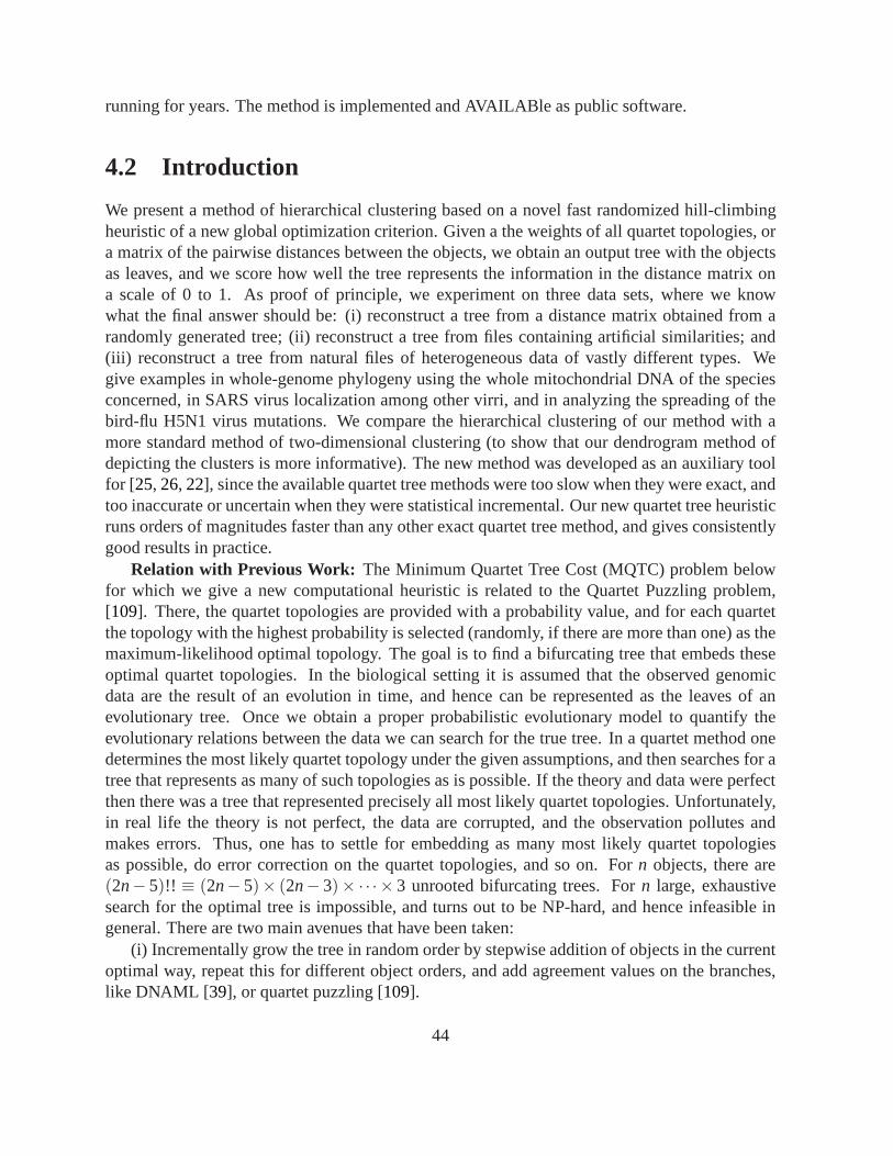
running for years. The method is implemented and AVAILABle as public software.
4.2 Introduction
We present a method of hierarchical clustering based on a novel fast randomized hill-climbingheuristic of a new global optimization criterion. Given a the weights of all quartet topologies, ora matrix of the pairwise distances between the objects, we obtain an output tree with the objectsas leaves, and we score how well the tree represents the information in the distance matrix ona scale of 0 to 1. As proof of principle, we experiment on threedata sets, where we knowwhat the final answer should be: (i) reconstruct a tree from a distance matrix obtained from arandomly generated tree; (ii) reconstruct a tree from files containing artificial similarities; and(iii) reconstruct a tree from natural files of heterogeneousdata of vastly different types. Wegive examples in whole-genome phylogeny using the whole mitochondrial DNA of the speciesconcerned, in SARS virus localization among other virri, and in analyzing the spreading of thebird-flu H5N1 virus mutations. We compare the hierarchical clustering of our method with amore standard method of two-dimensional clustering (to show that our dendrogram method ofdepicting the clusters is more informative). The new methodwas developed as an auxiliary toolfor [25, 26, 22], since the available quartet tree methods were too slow when they were exact, andtoo inaccurate or uncertain when they were statistical incremental. Our new quartet tree heuristicruns orders of magnitudes faster than any other exact quartet tree method, and gives consistentlygood results in practice.
Relation with Previous Work: The Minimum Quartet Tree Cost (MQTC) problem belowfor which we give a new computational heuristic is related tothe Quartet Puzzling problem,[109]. There, the quartet topologies are provided with a probability value, and for each quartetthe topology with the highest probability is selected (randomly, if there are more than one) as themaximum-likelihood optimal topology. The goal is to find a bifurcating tree that embeds theseoptimal quartet topologies. In the biological setting it isassumed that the observed genomicdata are the result of an evolution in time, and hence can be represented as the leaves of anevolutionary tree. Once we obtain a proper probabilistic evolutionary model to quantify theevolutionary relations between the data we can search for the true tree. In a quartet method onedetermines the most likely quartet topology under the givenassumptions, and then searches for atree that represents as many of such topologies as is possible. If the theory and data were perfectthen there was a tree that represented precisely all most likely quartet topologies. Unfortunately,in real life the theory is not perfect, the data are corrupted, and the observation pollutes andmakes errors. Thus, one has to settle for embedding as many most likely quartet topologiesas possible, do error correction on the quartet topologies,and so on. Forn objects, there are(2n− 5)!! ≡ (2n− 5)× (2n− 3)× ·· · × 3 unrooted bifurcating trees. Forn large, exhaustivesearch for the optimal tree is impossible, and turns out to beNP-hard, and hence infeasible ingeneral. There are two main avenues that have been taken:
(i) Incrementally grow the tree in random order by stepwise addition of objects in the currentoptimal way, repeat this for different object orders, and add agreement values on the branches,like DNAML [ 39], or quartet puzzling [109].
44
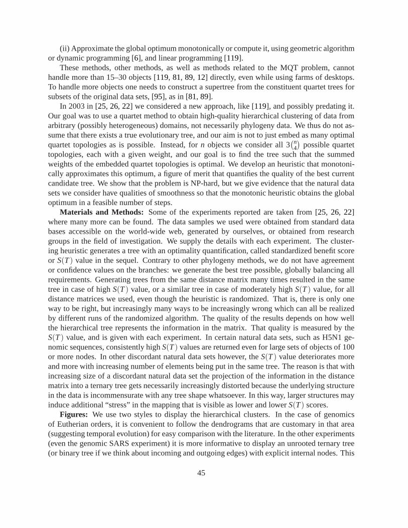
(ii) Approximate the global optimum monotonically or compute it, using geometric algorithmor dynamic programming [6], and linear programming [119].
These methods, other methods, as well as methods related to the MQT problem, cannothandle more than 15–30 objects [119, 81, 89, 12] directly, even while using farms of desktops.To handle more objects one needs to construct a supertree from the constituent quartet trees forsubsets of the original data sets, [95], as in [81, 89].
In 2003 in [25, 26, 22] we considered a new approach, like [119], and possibly predating it.Our goal was to use a quartet method to obtain high-quality hierarchical clustering of data fromarbitrary (possibly heterogeneous) domains, not necessarily phylogeny data. We thus do not as-sume that there exists a true evolutionary tree, and our aim is not to just embed as many optimalquartet topologies as is possible. Instead, forn objects we consider all 3
(n4
)possible quartet
topologies, each with a given weight, and our goal is to find the tree such that the summedweights of the embedded quartet topologies is optimal. We develop an heuristic that monotoni-cally approximates this optimum, a figure of merit that quantifies the quality of the best currentcandidate tree. We show that the problem is NP-hard, but we give evidence that the natural datasets we consider have qualities of smoothness so that the monotonic heuristic obtains the globaloptimum in a feasible number of steps.
Materials and Methods: Some of the experiments reported are taken from [25, 26, 22]where many more can be found. The data samples we used were obtained from standard databases accessible on the world-wide web, generated by ourselves, or obtained from researchgroups in the field of investigation. We supply the details with each experiment. The cluster-ing heuristic generates a tree with an optimality quantification, called standardized benefit scoreor S(T) value in the sequel. Contrary to other phylogeny methods, wedo not have agreementor confidence values on the branches: we generate the best tree possible, globally balancing allrequirements. Generating trees from the same distance matrix many times resulted in the sametree in case of highS(T) value, or a similar tree in case of moderately highS(T) value, for alldistance matrices we used, even though the heuristic is randomized. That is, there is only oneway to be right, but increasingly many ways to be increasingly wrong which can all be realizedby different runs of the randomized algorithm. The quality of the results depends on how wellthe hierarchical tree represents the information in the matrix. That quality is measured by theS(T) value, and is given with each experiment. In certain naturaldata sets, such as H5N1 ge-nomic sequences, consistently highS(T) values are returned even for large sets of objects of 100or more nodes. In other discordant natural data sets however, theS(T) value deteriorates moreand more with increasing number of elements being put in the same tree. The reason is that withincreasing size of a discordant natural data set the projection of the information in the distancematrix into a ternary tree gets necessarily increasingly distorted because the underlying structurein the data is incommensurate with any tree shape whatsoever. In this way, larger structures mayinduce additional “stress” in the mapping that is visible aslower and lowerS(T) scores.
Figures: We use two styles to display the hierarchical clusters. In the case of genomicsof Eutherian orders, it is convenient to follow the dendrograms that are customary in that area(suggesting temporal evolution) for easy comparison with the literature. In the other experiments(even the genomic SARS experiment) it is more informative todisplay an unrooted ternary tree(or binary tree if we think about incoming and outgoing edges) with explicit internal nodes. This
45
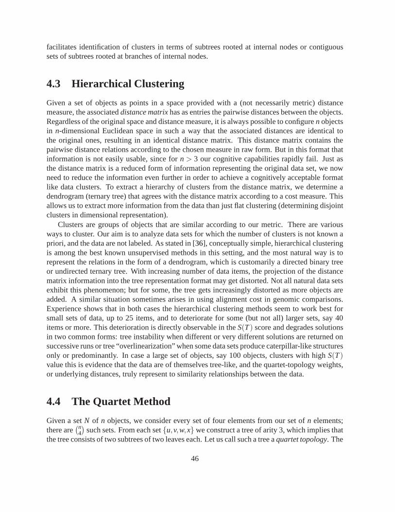
facilitates identification of clusters in terms of subtreesrooted at internal nodes or contiguoussets of subtrees rooted at branches of internal nodes.
4.3 Hierarchical Clustering
Given a set of objects as points in a space provided with a (notnecessarily metric) distancemeasure, the associateddistance matrixhas as entries the pairwise distances between the objects.Regardless of the original space and distance measure, it isalways possible to configuren objectsin n-dimensional Euclidean space in such a way that the associated distances are identical tothe original ones, resulting in an identical distance matrix. This distance matrix contains thepairwise distance relations according to the chosen measure in raw form. But in this format thatinformation is not easily usable, since forn > 3 our cognitive capabilities rapidly fail. Just asthe distance matrix is a reduced form of information representing the original data set, we nowneed to reduce the information even further in order to achieve a cognitively acceptable formatlike data clusters. To extract a hierarchy of clusters from the distance matrix, we determine adendrogram (ternary tree) that agrees with the distance matrix according to a cost measure. Thisallows us to extract more information from the data than justflat clustering (determining disjointclusters in dimensional representation).
Clusters are groups of objects that are similar according toour metric. There are variousways to cluster. Our aim is to analyze data sets for which the number of clusters is not known apriori, and the data are not labeled. As stated in [36], conceptually simple, hierarchical clusteringis among the best known unsupervised methods in this setting, and the most natural way is torepresent the relations in the form of a dendrogram, which iscustomarily a directed binary treeor undirected ternary tree. With increasing number of data items, the projection of the distancematrix information into the tree representation format mayget distorted. Not all natural data setsexhibit this phenomenon; but for some, the tree gets increasingly distorted as more objects areadded. A similar situation sometimes arises in using alignment cost in genomic comparisons.Experience shows that in both cases the hierarchical clustering methods seem to work best forsmall sets of data, up to 25 items, and to deteriorate for some(but not all) larger sets, say 40items or more. This deterioration is directly observable intheS(T) score and degrades solutionsin two common forms: tree instability when different or verydifferent solutions are returned onsuccessive runs or tree “overlinearization” when some datasets produce caterpillar-like structuresonly or predominantly. In case a large set of objects, say 100objects, clusters with highS(T)value this is evidence that the data are of themselves tree-like, and the quartet-topology weights,or underlying distances, truly represent to similarity relationships between the data.
4.4 The Quartet Method
Given a setN of n objects, we consider every set of four elements from our set of n elements;there are
(n4
)such sets. From each setu,v,w,xwe construct a tree of arity 3, which implies that
the tree consists of two subtrees of two leaves each. Let us call such a tree aquartet topology. The
46

set of 3(n
4
)quartet topologies induced byN is denoted byQ. We denote a partitionu,v,w,x
of u,v,w,x by uv|wx. There are three possibilities to partitionu,v,w,x into two subsets oftwo elements each: (i)uv|wx, (ii) uw|vx, and (iii)ux|vw. In terms of the tree topologies: a verticalbar divides the two pairs of leaf nodes into two disjoint subtrees (Figure4.1).
un0
v
wn1
x
u
n0
v
n1
w
x
un0
vn1
w
x
Figure 4.1: The three possible quartet topologies for the set of leaf labelsu,v,w,x.
4.4.1.DEFINITION. Define abinary dendrogramas an element from the classT of undirectedtrees of arity 3 withn≥ 4 leaves, labeled with the elements ofN.
Such trees haven leaves andn−2 internal nodes. For any given treeT from this class, and anyset of four leaf labelsu,v,w,x∈N, we sayT is consistentwith uv|wx if and only if the path fromu to v does not cross the path fromw to x. It is easy to see that precisely one of the three possiblequartet topologies for any set of 4 labels is consistent for agiven tree from the above class, andtherefore a tree fromT contains precisely
(n4
)different quartet topologies. We may think of a
large tree having many smaller quartet topologies embeddedwithin its structure. Commonly thegoal in the quartet method is to find (or approximate as closely as possible) the tree that embedsthe maximal number of consistent (possibly weighted) quartet topologies from a given setP⊆Qof quartet topologies [53] (Figure 4.2). A weight function W: P→ R , with R the set of realnumbers determines the weights. The unweighted case is whenW(uv|wx) = 1 for all uv|wx∈ P.
4.4.2.DEFINITION. The (weighted)Maximum Quartet Consistency (MQC)is defined as fol-lows:
GIVEN: N, P, andW.QUESTION: FindT0 = maxT ∑W(uv|wx) : uv|wx∈ P anduv|wx is consistent withT.
47
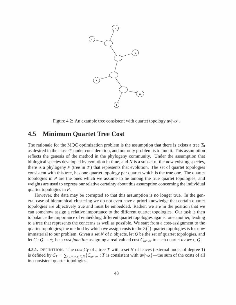
u
s
v
x
w
t
Figure 4.2: An example tree consistent with quartet topology uv|wx .
4.5 Minimum Quartet Tree Cost
The rationale for the MQC optimization problem is the assumption that there is exists a treeT0
as desired in the classT under consideration, and our only problem is to find it. This assumptionreflects the genesis of the method in the phylogeny community. Under the assumption thatbiological species developed by evolution in time, andN is a subset of the now existing species,there is a phylogenyP (tree inT ) that represents that evolution. The set of quartet topologiesconsistent with this tree, has one quartet topology per quartet which is the true one. The quartettopologies inP are the ones which we assume to be among the true quartet topologies, andweights are used to express our relative certainty about this assumption concerning the individualquartet topologies inP.
However, the data may be corrupted so that this assumption isno longer true. In the gen-eral case of hierarchical clustering we do not even have a priori knowledge that certain quartettopologies are objectively true and must be embedded. Rather, we are in the position that wecan somehow assign a relative importance to the different quartet topologies. Our task is thento balance the importance of embedding different quartet topologies against one another, leadingto a tree that represents the concerns as well as possible. Westart from a cost-assignment to thequartet topologies; the method by which we assign costs to the 3
(n4
)quartet topologies is for now
immaterial to our problem. Given a setN of n objects, letQ be the set of quartet topologies, andlet C : Q→ R be acost functionassigning a real valued costCuv|wx to each quartetuv|wx∈Q.
4.5.1.DEFINITION. Thecost CT of a treeT with a setN of leaves (external nodes of degree 1)is defined byCT = ∑u,v,w,x⊆NCuv|wx : T is consistent withuv|wx—the sum of the costs of allits consistent quartet topologies.
48
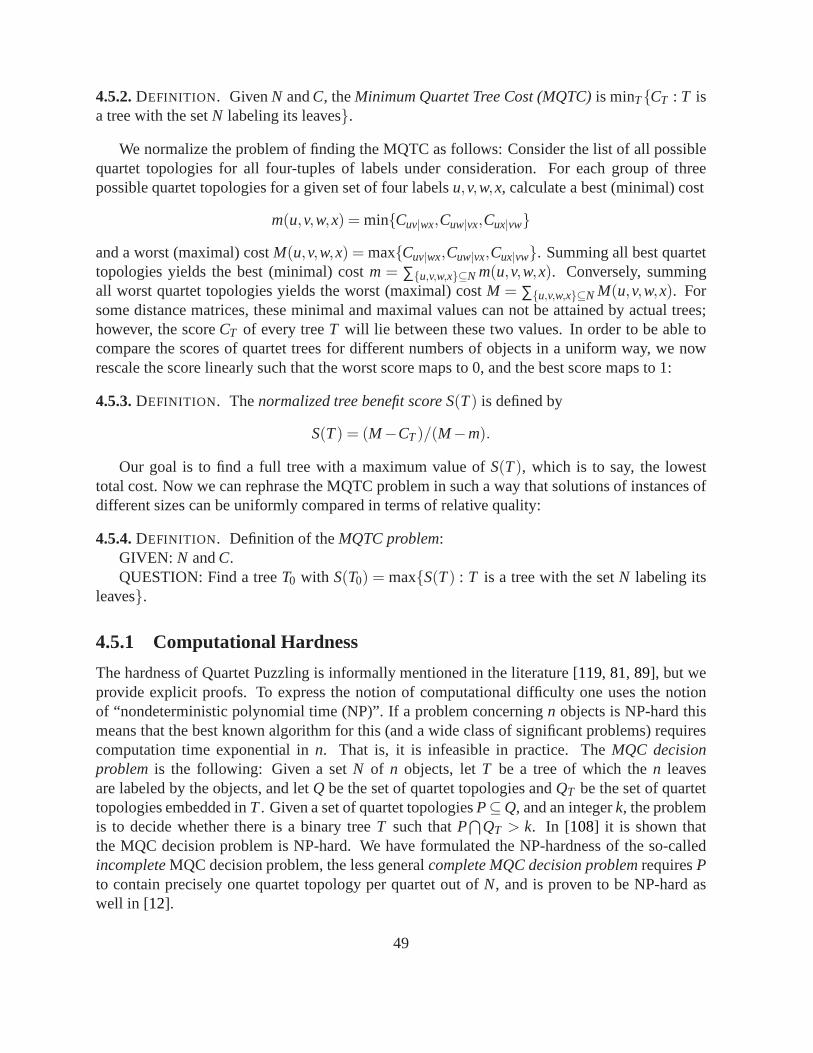
4.5.2.DEFINITION. GivenN andC, theMinimum Quartet Tree Cost (MQTC)is minTCT : T isa tree with the setN labeling its leaves.
We normalize the problem of finding the MQTC as follows: Consider the list of all possiblequartet topologies for all four-tuples of labels under consideration. For each group of threepossible quartet topologies for a given set of four labelsu,v,w,x, calculate a best (minimal) cost
m(u,v,w,x) = minCuv|wx,Cuw|vx,Cux|vw
and a worst (maximal) costM(u,v,w,x) = maxCuv|wx,Cuw|vx,Cux|vw. Summing all best quartettopologies yields the best (minimal) costm = ∑u,v,w,x⊆N m(u,v,w,x). Conversely, summingall worst quartet topologies yields the worst (maximal) cost M = ∑u,v,w,x⊆N M(u,v,w,x). Forsome distance matrices, these minimal and maximal values can not be attained by actual trees;however, the scoreCT of every treeT will lie between these two values. In order to be able tocompare the scores of quartet trees for different numbers ofobjects in a uniform way, we nowrescale the score linearly such that the worst score maps to 0, and the best score maps to 1:
4.5.3.DEFINITION. Thenormalized tree benefit score S(T) is defined by
S(T) = (M−CT)/(M−m).
Our goal is to find a full tree with a maximum value ofS(T), which is to say, the lowesttotal cost. Now we can rephrase the MQTC problem in such a way that solutions of instances ofdifferent sizes can be uniformly compared in terms of relative quality:
4.5.4.DEFINITION. Definition of theMQTC problem:GIVEN: N andC.QUESTION: Find a treeT0 with S(T0) = maxS(T) : T is a tree with the setN labeling its
leaves.
4.5.1 Computational Hardness
The hardness of Quartet Puzzling is informally mentioned inthe literature [119, 81, 89], but weprovide explicit proofs. To express the notion of computational difficulty one uses the notionof “nondeterministic polynomial time (NP)”. If a problem concerningn objects is NP-hard thismeans that the best known algorithm for this (and a wide classof significant problems) requirescomputation time exponential inn. That is, it is infeasible in practice. TheMQC decisionproblem is the following: Given a setN of n objects, letT be a tree of which then leavesare labeled by the objects, and letQ be the set of quartet topologies andQT be the set of quartettopologies embedded inT. Given a set of quartet topologiesP⊆Q, and an integerk, the problemis to decide whether there is a binary treeT such thatP
T
QT > k. In [108] it is shown thatthe MQC decision problem is NP-hard. We have formulated the NP-hardness of the so-calledincompleteMQC decision problem, the less generalcomplete MQC decision problemrequiresPto contain precisely one quartet topology per quartet out ofN, and is proven to be NP-hard aswell in [12].
49

4.5.5.THEOREM. The MQTC decision problem is NP-hard.
PROOF. By reduction from the MQC decision problem. For every MQC decision problem onecan define a corresponding MQTC decision problem that has thesame solution: give the quartettopologies inP cost 0 and the ones inQ−P cost 1. Consider the MQTC decision problem: isthere a treeT with the setN labeling its leaves such thatCT <
(n4
)−k? An alternative equivalent
formulation is: is there a treeT with the setN labeling its leaves such that
S(T) >M−
(n4
)+k
M−m?
Note that every treeT with the setN labeling its leaves has precisely one out of the three quartettopologies of every of the
(n4
)quartets embedded in it. Therefore, the costCT =
(n4
)−|PT
QT |.If the answer to the above question is affirmative, then the number of quartet topologies inPthat are embedded in the tree exceedsk; if it is not then there is no tree such that the number ofquartet topologies inP embedded in it exceedsk. This way the MQC decision problem can bereduced to the MQTC decision problem, which shows also the latter to be NP-hard. 2
Is it possible that the bestS(T) value is always one, that is, there always exists a tree thatembeds all quartets at minimum cost quartet topologies? Consider the casen = |N| = 4. Sincethere is only one quartet, we can setT0 equal to the minimum cost quartet topology, and haveS(T0) = 1. A priori we cannot exclude the possibility that for everyN andC there always is atreeT0 with S(T0) = 1. In that case, the MQTC Problem reduces to finding thatT0. However,the situation turns out to be more complex. Note first that theset of quartet topologies uniquelydetermines a tree inT , [15].
4.5.6.LEMMA . Let T,T′ be different labeled trees inT and let QT ,QT′ be the sets of embeddedquartet topologies, respectively. Then, QT 6= QT ′.
A complete setof quartet topologies onN is a set containing precisely one quartet topology
per quartet. There are 3(n4) such combinations, but only 2(
n2) labeled undirected graphs onn nodes
(and therefore|T | ≤ 2(n2)). Hence, not every complete set of quartet topologies corresponds to
a tree inT . This already suggests that we can weight the quartet topologies in such a way thatthe full combination of all quartet topologies at minimal costs does not correspond to a tree inT , and henceS(T0) < 1 for T0 ∈ T realizing the MQTC optimum. For an explicit example ofthis, we use that a complete set corresponding to a tree inT must satisfy certain transitivityproperties, [29, 28]:
4.5.7.LEMMA . Let T be a tree in the considered class with leaves N, Q the set of quartet topolo-gies and Q0⊆Q. Then Q0 uniquely determines T if
(i) Q0 contains precisely one quartet topology for every quartet,and(ii) For all a,b,c,d,e⊆N, if ab|bc,ab|de∈Q then ab|ce∈Q, as well as if ab|cd,bc|de∈Q
then ab|de∈Q.
50

4.5.8.THEOREM. There are N (with n= |N| = 5) and a cost function C such that, for everyT ∈ T , S(T) does not exceed4/5.
PROOF. ConsiderN = u,v,w,x,y andC(uv|wx) = 1− ε(ε > 0),C(uw|xv) = C(ux|vw) = 0,C(xy|uv) = C(wy|uv) = C(uy|wx) = C(vy|wx) = 0, andC(ab|cd) = 1 for all remaining quartettopologiesab|cd∈ Q. We see thatM = 5− ε, m= 0. The treeT0 = (y,((u,v),(w,x))) has costCT0 = 1− ε, since it embeds quartet topologiesuw|xv,xy|uv,wy|uv,uy|wx,vy|wx. We show thatT0 achieves the MQTC optimum.Case 1:If a treeT 6= T0 embedsuv|wx, then it must by Item(i) of Lemma4.5.7also embed a quartet topology containingy that has cost 1.
Case 2:If a treeT 6= T0 embedsuw|xvandxy|uv, then it must by Item (ii) of the Lemma4.5.7also embeduw|xy, and hence have costCT ≥ 1. Similarly, all other remaining cases of embeddinga combination of a quartet topology not containingy of 0 cost with a quartet topology containingy of 0 cost inT, imply an embedded quartet topology of cost 1 inT. 2
Altogether, the MQTC optimization problem is infeasible inpractice, and natural data canhave an optimalS(T) < 1. In fact, it follows from the above analysis that to determineS(T) ingeneral is NP-hard. In [12] a polynomial time approximation scheme for complete MQC isex-hibited, a theoretical approximation scheme allowing the approximation of the optimal solutionup to arbitrary precision, with running time polynomial in the inverse of that precision. We say“theoretical” since that algorithm would run in something like n19. For incomplete MQC it isshown that even such a theoretical algorithm does not exist,unless P=NP. Hence, computationof the MQTC optimum, and even its approximation with given precision, requires superpolyno-mial time unless P=NP. Therefore, any practical approach toobtain or approximate the MQTCoptimum requires heuristics.
4.6 New Heuristic
Our algorithm is essentially randomized hill-climbing, using parallellized Genetic Programming,where undirected trees evolve in a random walk driven by a prescribed fitness function. We aregiven a setN of n objects and a weighting functionW.
4.6.1.DEFINITION. We define asimple mutationon a labeled undirected ternary tree as one ofthree possible transformations:
1. A leaf swap, which consists of randomly choosing two leaf nodes and swapping them.
2. A subtree swap, which consists of randomly choosing two internal nodes andswappingthe subtrees rooted at those nodes.
3. A subtree transfer, whereby a randomly chosen subtree (possibly a leaf) is detached andreattached in another place, maintaining arity invariants.
Each of these simple mutations keeps the number of leaf nodesand internal nodes in the treeinvariant; only the structure and placements change.
4.6.2.DEFINITION. A k-mutationis a sequence ofk simple mutations. Thus, a simple mutationis a 1-mutation.
51
4.6.1 Algorithm
Step 1: First, a random treeT ∈ T with 2n−2 nodes is created, consisting ofn leaf nodes (with1 connecting edge) labeled with the names of the data items, andn−2 non-leaf orinternalnodeslabeled with the lowercase letter “k” followed by a unique integer identifier. Each internal nodehas exactly three connecting edges.
Step 2: For this treeT, we calculate the total cost of all embedded quartet topologies, com-puteS(T).
Comment:A tree is consistent with precisely13 of all quartet topologies, one for every quartet.A random tree is likely to be consistent with about1
3 of the best quartet topologies—but this isnecessarily imprecise because of dependencies.
Step 3: Thecurrently best known treevariableT0 is set toT: T0← T.Comment:ThisT0 is used as the basis for further searching.Step 4:Pick a numberk with probabilityp(k) = c/(k(logk)2) where 1/c= ∑∞
k=11/(k(logk)2).Comment:This numberk is the number of simple mutations that we will perform in the
nextk-mutation. The probability distributionp(k) is easily generated by running a random fairbit generator and setk to the length of the first self-delimiting sequence generated. That is, ifx = x1 . . .xk ∈ 0,1k (|x| = k≥ 1), then ¯x = 1k−10x, x′ = |x|x, andx′′ = |x′|x′. Thus, the length|x′′|= k+ logk+2log logk. The probability of generatingx′′ corresponding to a givenx of lengthk by fair coin flips is 2−|x
′′| = 2−k−logk−2log logk = 2−k/(k(logk)2). The probability of generatingx′′ corresponding tosome xof lengthk is 2k times as large, that is, 1/(k(logk)2). In practice, weused a “shifted” fat tail distribution 1/((k+2)(logk+2)2)
Step 5: Compose ak-mutation by, for each such simple mutation, choosing one ofthe threetypes listed above with equal probability. For each of thesesimple mutations, we uniformly atrandom select leaves or internal nodes, as appropriate.
Comment:Notice that trees which are close to the original tree (in terms of number of simplemutation steps in between) are examined often, while trees that are far away from the originaltree will eventually be examined, but not very frequently.
Step 6: In order to search for a better tree, we simply apply thek-mutation constructed inStep 5on T0 to obtainT ′, and then calculateS(T′). If S(T′) ≥ S(T0), then replace the currentcandidate inT0 by T (as the new best tree):T0← T.
Step 7: If S(T0) = 1 or atermination condition to be discussed below holds, then output thetree inT0 as the best tree and halt. Otherwise, go toStep 4.
4.6.3.REMARK . We have chosenp(k) to be a “fat-tail” distribution, with the fattest tail possible,so that we may concentrate maximal probability also on the larger values ofk. That way, thelikelihood of getting trapped in local minima is minimized.In contrast, if one would choose anexponential scheme, likeq(k) = ce−k, then the larger values ofk would arise so scarcely thatpractically speaking the distinction between being absolutely trapped in a local optimum, andthe very low escape probability, would be insignificant. Considering positive-valued probabilitymass functionsq : N → (0,1], with N the natural numbers, as we do here, we note that such afunction (i) limk→∞ q(k) = 0, and (ii)∑∞
k=1q(k) = 1. Thus, every function of the natural numbersthat has strictly positive values and converges can be normalized to such a probability mass
52
function. For smooth analytic functions that can be expressed a series of fractional powers andlogarithms, the borderline between converging and diverging is as follows:∑1/k,∑1/(k logk),∑1/(k logk loglogk) and so on diverge, while∑1/k2,∑1/(k(logk)2),∑1/(k logk(loglogk)2)and so on converge. Therefore, the maximal fat tail of a “smooth” function f (x) with ∑ f (x) < ∞arises for functions at the edge of the convergence family. The distributionp(k) = c/(k(logk)2)is as close to the edge as is reasonable, and because the used coding x→ x′′ is a prefix codewe have∑1/(k(logk)2)≤ 1 by the Kraft Inequality (see for example [79]) and thereforec≥ 1.Let us see what this means for our algorithm using the chosen distribution p(k). For N = 64,say, we can change any tree inT to any other tree inT with a 64-mutation. The probabilityof such a complex mutation occurring is quite large with sucha fat tail: 1/(64·62) = 1/2304,that is, more than 40 times in 100,000 generations. If we can get out of a local minimum withalready a 32-mutation, then this occurs with probability atleast 1/800, so 125 times, and with a16-mutation with probability at least 1/196, so 510 times.
4.6.2 Performance
The main problem with hill-climbing algorithms is that theycan get stuck in a local optimum.However, by randomly selecting a sequence of simple mutations, longer sequences with de-creasing probability, we essentially run a Metropolis Monte Carlo algorithm [83], reminiscentof simulated annealing [56] at random temperatures. Since there is a nonzero probability forevery tree inT being transformed into every other tree inT , there is zero probability that we gettrapped forever in a local optimum that is not a global optimum. That is, trivially:
4.6.4.LEMMA . (i) The algorithm approximates the MQTC optimal solution monotonically ineach run.
(ii) The algorithm without termination condition solves the MQTC optimization problemeventually with probability 1 (but we do not in general know when the optimum has been reachedin a particular run).
The main question therefore is the convergence speed of the algorithm on natural data, anda termination criterion to terminate the algorithm when we have an acceptable approximation.From the impossibility result in [12] we know that there is no polynomial approximation schemefor MQTC optimization, and whether our scheme is expected polynomial time seems to requireproving that the involved Metropolis chain is rapidly mixing [116], a notoriously hard and gen-erally unsolved problem. In practice, in our experiments there is unanimous evidence that forthe natural data and the weighting function we have used, convergence is always fast. We haveto determine the cost of
(n4
)quartets to determine eachS(T) value. Hence the algorithm runs in
time at least that much. In experiments we found that for the same data set different runs con-sistently showed the same behavior, for example Figure4.3 for a 60-object computation. Therethe S(T) value leveled off at about 70,000 examined trees, and the termination condition was“no improvement in 5,000 trees.” Different random runs of the algorithm nearly always gave thesame behavior, returning a tree with the sameS(T) value, albeit a different tree in most caseswith hereS(T)≈ 0.865, a relatively low value. That is, since there are many ways to find a treeof optimalS(T) value, and apparently the algorithm never got trapped in a lower local optimum.
53

0
0.1
0.2
0.3
0.4
0.5
0.6
0.7
0.8
0.9
0 10000 20000 30000 40000 50000 60000 70000 80000
S(T)
Total trees examined
’gnup.dat’
Figure 4.3: Progress of a 60-item data set experiment over time.
For problems with highS(T) value, as we see later, the algorithm consistently returnedthe sametree. This situation is perhaps similar to the behavior of the Simplex method in linear program-ming, that can be shown to run in exponential time on a badly chosen problem instance, but inpractice on natural problems consistently runs in linear time.
Note that if a tree is ever found such thatS(T) = 1, then we can stop because we can becertain that this tree is optimal, as no tree could have a lower cost. In fact, this perfect tree resultis achieved in our artificial tree reconstruction experiment (Section4.6.5) reliably in a few min-utes. For real-world data,S(T) reaches a maximum somewhat less than 1, presumably reflectingdistortion of the information in the distance matrix data bythe best possible tree representation,as noted above, or indicating getting stuck in a local optimum or a search space too large tofind the global optimum. On many typical problems of up to 40 objects this tree-search gives atree withS(T) ≥ 0.9 within half an hour. For large numbers of objects, tree scoring itself canbe slow: as this takes ordern4 computation steps. Current single computers can score a tree ofthis size in about a minute. Additionally, the space of treesis large, so the algorithm may slowdown substantially. For larger experiments, we used the C program called partree (part of theCompLearn package [21]) with MPI (Message Passing Interface, a common standard used onmassively parallel computers) on a cluster of workstationsin parallel to find trees more rapidly.We can consider the graph mapping the achievedS(T) score as a function of the number oftrees examined. Progress occurs typically in a sigmoidal fashion towards a maximal value≤ 1,Figure4.3.
54
4.6.3 Termination Condition
The termination conditionis of two types and which type is used determines the number ofobjects we can handle.
Simple termination condition:We simply run the algorithm until it seems no better trees arebeing found in a reasonable amount of time. Here we typicallyterminate if no improvement inS(T) value is achieved within 100,000 examined trees. This criterion is simple enough to enableus to hierarchically cluster data sets up to 80 objects in a few hours. This is way above the 15–30objects in the previous exact (non-incremental) methods (see Introduction).
Agreement termination condition:In this more sophisticated method we select a number2≤ r ≤ 6 of runs, and we runr invocations of the algorithm in parallel. Each time anS(T) valuein run i = 1, . . . , r is increased in this process it is compared with theS(T) values in all the otherruns. If they are all equal, then the candidate trees of the runs are compared. This can be doneby simply comparing the ordered lists of embedded quartet topologies, in some standard order,since the set of embedded quartet topologies uniquely determines the quartet tree by [15]. If ther candidate trees are identical, then terminate with this quartet tree as output, otherwise continuethe algorithm.
This termination condition takes (for the same number of steps per run) aboutr times aslong as the simple termination condition. But the termination condition is much more rigorous,provided we chooser appropriate to the numbern of objects being clustered. Since all the runsare randomized independently at startup, it seems very unlikely that with natural data all of themget stuck in the same local optimum with the same quartet treeinstance, provided the numbernof objects being clustered is not too small. Forn = 5 and the number of invocationsr = 2, thereis a reasonable probability that the two different runs by chance hit the same tree in the samestep. This phenomenon leads us to require more than two successive runs with exact agreementbefore we may reach a final answer for smalln. In the case of 4≤ n≤ 5, we require 6 dovetailedruns to agree precisely before termination. For 6≤ n≤ 9, r = 5. For 10≤ n≤ 15, r = 4. For16≤ n≤ 17, r = 3. For all othern≥ 18, r = 2. This yields a reasonable tradeoff between speedand accuracy.
It is clear that there is only one tree withS(T) = 1 (if that is possible for the data), and randomtrees (the majority of all possible quartet trees) haveS(T) ≈ 1/3 (above). This gives evidencethat the number of quartet trees with largeS(T) values is much smaller than the number of treeswith smallS(T) values. It is furthermore evident that the precise relationdepends on the data setinvolved, and hence cannot be expressed by a general formulawithout further assumptions on thedata. However, we can safely state that small data sets, of say≤ 15 objects, that in our experienceoften lead toS(T) values close to 1 have very few quartet trees realizing the optimal S(T) value.On the other hand, those large sets of 60 or more objects that contain some inconsistency andthus lead to a low finalS(T) value also tend to exhibit more variation as one might expect. Thissuggests that in the agreement termination method each run will get stuck in a different quartettree of a similarS(T) value, so termination with the same tree is not possible. Experiments showthat with the rigorous agreement termination we can handle sets of up to 40 objects, and withthe simple termination up to at least 80 objects on a single computer or 100-200 objects using acluster of computers in parallel.
55

4.6.4 Tree Building Statistics
We used the CompLearn package, (further described in Chapter 10) [21], to analyze a “10-mammals” example withzlib compression yielding a 10× 10 distance matrix, similar to theexamples in Section4.10. The algorithm starts with four randomly initialized trees. It tries toimprove each one randomly and finishes when they match. Thus,every run produces an outputtree, a maximum score associated with this tree, and has examined some total number of trees,T, before it finished. Figure4.4 shows a graph displaying a histogram ofT over one thousandruns of the distance matrix. Thex-axis represents a number of trees examined in a single runof the program, measured in thousands of trees and binned in 1000-wide histogram bars. Themaximum number is about 12000 trees examined. The graph suggests a Poisson distribution.
0
50
100
150
200
250
300
0 2 4 6 8 10 12
runs
thousands of trees examined for a single run
run length histogram
Figure 4.4: Histogram of run-time number of trees examined before termination.
About 2/3rd of the trials take less than 4000 trees. In the thousand trials above, 994 ended withthe optimalS(T) = 0.999514. The remaining six runs returned 5 cases of the second-highestscore,S(T) = 0.995198 and one case ofS(T) = 0.992222. It is important to realize that outcomestability is dependent on input matrix particulars.
Another interesting distribution is the mutation stepsize. Recall that the mutation length isdrawn from a shifted fat-tail distribution. But if we restrict our attention to just the mutationsthat improve theS(T) value, then we may examine these statistics to look for evidence of amodification to this distribution due to, for example, the presence of very many isolated areas thathave only long-distance ways to escape. Figure4.5shows the histogram of successful mutationlengths (that is, number of simple mutations composing a single complex mutation) and rejectedlengths (both normalized) which shows that this is not the case. Here thex-axis is the number ofmutation steps and they-axis is the normalized proportion of times that step size occurred. Thisgives good empirical evidence that in this case, at least, wehave a relatively easy search space,without large gaps.
56
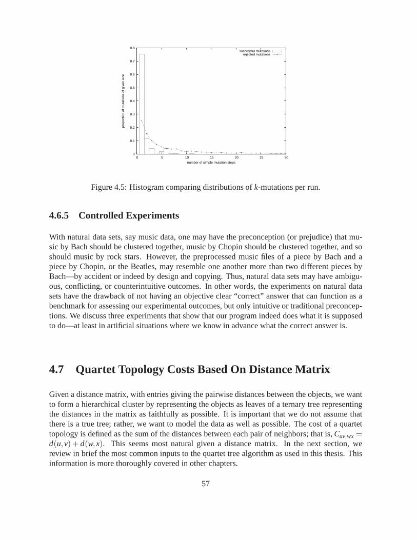
0
0.1
0.2
0.3
0.4
0.5
0.6
0.7
0.8
0 5 10 15 20 25 30
prop
ortio
n of
mut
atio
ns o
f giv
en s
ize
number of simple mutation steps
successful mutationsrejected mutations
Figure 4.5: Histogram comparing distributions ofk-mutations per run.
4.6.5 Controlled Experiments
With natural data sets, say music data, one may have the preconception (or prejudice) that mu-sic by Bach should be clustered together, music by Chopin should be clustered together, and soshould music by rock stars. However, the preprocessed musicfiles of a piece by Bach and apiece by Chopin, or the Beatles, may resemble one another more than two different pieces byBach—by accident or indeed by design and copying. Thus, natural data sets may have ambigu-ous, conflicting, or counterintuitive outcomes. In other words, the experiments on natural datasets have the drawback of not having an objective clear “correct” answer that can function as abenchmark for assessing our experimental outcomes, but only intuitive or traditional preconcep-tions. We discuss three experiments that show that our program indeed does what it is supposedto do—at least in artificial situations where we know in advance what the correct answer is.
4.7 Quartet Topology Costs Based On Distance Matrix
Given a distance matrix, with entries giving the pairwise distances between the objects, we wantto form a hierarchical cluster by representing the objects as leaves of a ternary tree representingthe distances in the matrix as faithfully as possible. It is important that we do not assume thatthere is a true tree; rather, we want to model the data as well as possible. The cost of a quartettopology is defined as the sum of the distances between each pair of neighbors; that is,Cuv|wx =d(u,v) + d(w,x). This seems most natural given a distance matrix. In the nextsection, wereview in brief the most common inputs to the quartet tree algorithm as used in this thesis. Thisinformation is more thoroughly covered in other chapters.
57
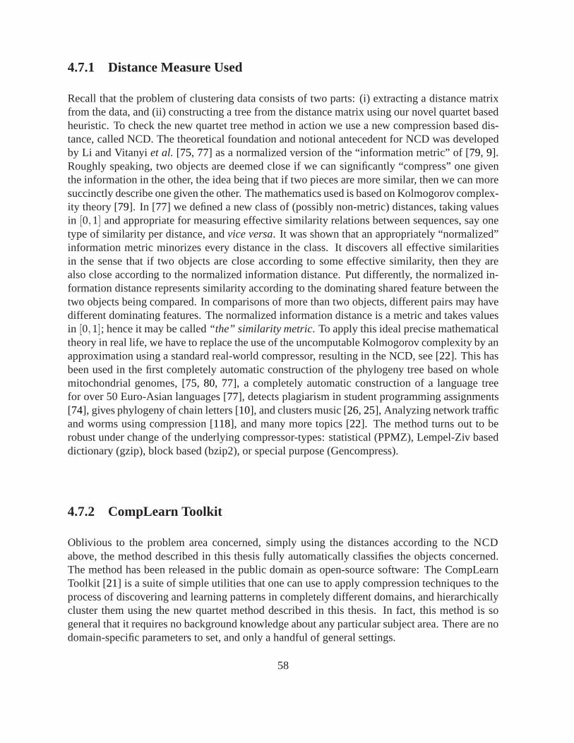
4.7.1 Distance Measure Used
Recall that the problem of clustering data consists of two parts: (i) extracting a distance matrixfrom the data, and (ii) constructing a tree from the distancematrix using our novel quartet basedheuristic. To check the new quartet tree method in action we use a new compression based dis-tance, called NCD. The theoretical foundation and notionalantecedent for NCD was developedby Li and Vitanyiet al. [75, 77] as a normalized version of the “information metric” of [79, 9].Roughly speaking, two objects are deemed close if we can significantly “compress” one giventhe information in the other, the idea being that if two pieces are more similar, then we can moresuccinctly describe one given the other. The mathematics used is based on Kolmogorov complex-ity theory [79]. In [77] we defined a new class of (possibly non-metric) distances, taking valuesin [0,1] and appropriate for measuring effective similarity relations between sequences, say onetype of similarity per distance, andvice versa. It was shown that an appropriately “normalized”information metric minorizes every distance in the class. It discovers all effective similaritiesin the sense that if two objects are close according to some effective similarity, then they arealso close according to the normalized information distance. Put differently, the normalized in-formation distance represents similarity according to thedominating shared feature between thetwo objects being compared. In comparisons of more than two objects, different pairs may havedifferent dominating features. The normalized information distance is a metric and takes valuesin [0,1]; hence it may be called“the” similarity metric. To apply this ideal precise mathematicaltheory in real life, we have to replace the use of the uncomputable Kolmogorov complexity by anapproximation using a standard real-world compressor, resulting in the NCD, see [22]. This hasbeen used in the first completely automatic construction of the phylogeny tree based on wholemitochondrial genomes, [75, 80, 77], a completely automatic construction of a language treefor over 50 Euro-Asian languages [77], detects plagiarism in student programming assignments[74], gives phylogeny of chain letters [10], and clusters music [26, 25], Analyzing network trafficand worms using compression [118], and many more topics [22]. The method turns out to berobust under change of the underlying compressor-types: statistical (PPMZ), Lempel-Ziv baseddictionary (gzip), block based (bzip2), or special purpose(Gencompress).
4.7.2 CompLearn Toolkit
Oblivious to the problem area concerned, simply using the distances according to the NCDabove, the method described in this thesis fully automatically classifies the objects concerned.The method has been released in the public domain as open-source software: The CompLearnToolkit [21] is a suite of simple utilities that one can use to apply compression techniques to theprocess of discovering and learning patterns in completelydifferent domains, and hierarchicallycluster them using the new quartet method described in this thesis. In fact, this method is sogeneral that it requires no background knowledge about any particular subject area. There are nodomain-specific parameters to set, and only a handful of general settings.
58
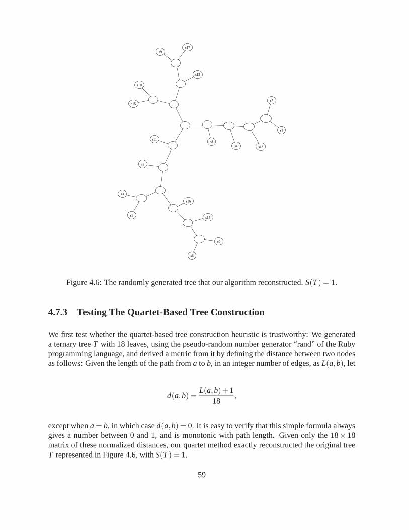
s0
s6
s1
s7
s2
s3
s5
s4
s8
s9
s17
s10
s15
s11
s12
s13
s14
s16
Figure 4.6: The randomly generated tree that our algorithm reconstructed.S(T) = 1.
4.7.3 Testing The Quartet-Based Tree Construction
We first test whether the quartet-based tree construction heuristic is trustworthy: We generateda ternary treeT with 18 leaves, using the pseudo-random number generator “rand” of the Rubyprogramming language, and derived a metric from it by defining the distance between two nodesas follows: Given the length of the path froma to b, in an integer number of edges, asL(a,b), let
d(a,b) =L(a,b)+1
18,
except whena = b, in which cased(a,b) = 0. It is easy to verify that this simple formula alwaysgives a number between 0 and 1, and is monotonic with path length. Given only the 18×18matrix of these normalized distances, our quartet method exactly reconstructed the original treeT represented in Figure4.6, with S(T) = 1.
59

a
ac
ab
abc
abcd
abce
abe
abfg
acfg
abhi
abhj
c
e
d
g
f
h
hijk
jk
i
ij
j
Figure 4.7: Classification of artificial files with repeated 1-kilobyte tags. Not all possibilities areincluded; for example, file “b” is missing.S(T) = 0.905.
4.8 Testing On Artificial Data
Given that the tree reconstruction method is accurate on clean consistent data, we tried whetherthe full procedure works in an acceptable manner when we knowwhat the outcome should belike. We used the “rand” pseudo-random number generator from the C programming languagestandard library under Linux. We randomly generated 11 separate 1-kilobyte blocks of datawhere each byte was equally probable and called thesetags. Each tag was associated with adifferent lowercase letter of the alphabet. Next, we generated 22 files of 80 kilobyte each, bystarting with a block of purely random bytes and applying one, two, three, or four differenttags on it. Applying a tag consists of ten repetitions of picking a random location in the 80-kilobyte file, and overwriting that location with the globally consistent tag that is indicated. So,for instance, to create the file referred to in the diagram by “a,” we start with 80 kilobytes ofrandom data, then pick ten places to copy over this random data with the arbitrary 1-kilobytesequence identified as taga. Similarly, to create file “ab,” we start with 80 kilobytes ofrandomdata, then pick ten places to put copies of taga, then pick ten more places to put copies of tagb (perhaps overwriting some of thea tags). Because we never use more than four different tags,and therefore never place more than 40 copies of tags, we can expect that at least half of the datain each file is random and uncorrelated with the rest of the files. The rest of the file is correlated
60
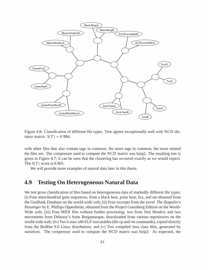
ELFExecutableA
ELFExecutableB
GenesBlackBearA
GenesPolarBearB
GenesFoxC
GenesRatD
JavaClassA
JavaClassB
MusicBergA
MusicBergB
MusicHendrixA
MusicHendrixB
TextA
TextB
TextC
TextD
Figure 4.8: Classification of different file types. Tree agrees exceptionally well with NCD dis-tance matrix:S(T) = 0.984.
with other files that also contain tags in common; the more tags in common, the more relatedthe files are. The compressor used to compute the NCD matrix was bzip2. The resulting tree isgiven in Figure4.7; it can be seen that the clustering has occurred exactly as wewould expect.TheS(T) score is 0.905.
We will provide more examples of natural data later in this thesis.
4.9 Testing On Heterogeneous Natural Data
We test gross classification of files based on heterogeneous data of markedly different file types:(i) Four mitochondrial gene sequences, from a black bear, polar bear, fox, and rat obtained fromthe GenBank Database on the world-wide web; (ii) Four excerpts from the novelThe Zeppelin’sPassengerby E. Phillips Oppenheim, obtained from the Project Gutenberg Edition on the World-Wide web; (iii) Four MIDI files without further processing; two from Jimi Hendrix and twomovements from Debussy’s Suite Bergamasque, downloaded from various repositories on theworld-wide web; (iv) Two Linux x86 ELF executables (thecpandrmcommands), copied directlyfrom the RedHat 9.0 Linux distribution; and (v) Two compiledJava class files, generated byourselves. The compressor used to compute the NCD matrix wasbzip2. As expected, the
61
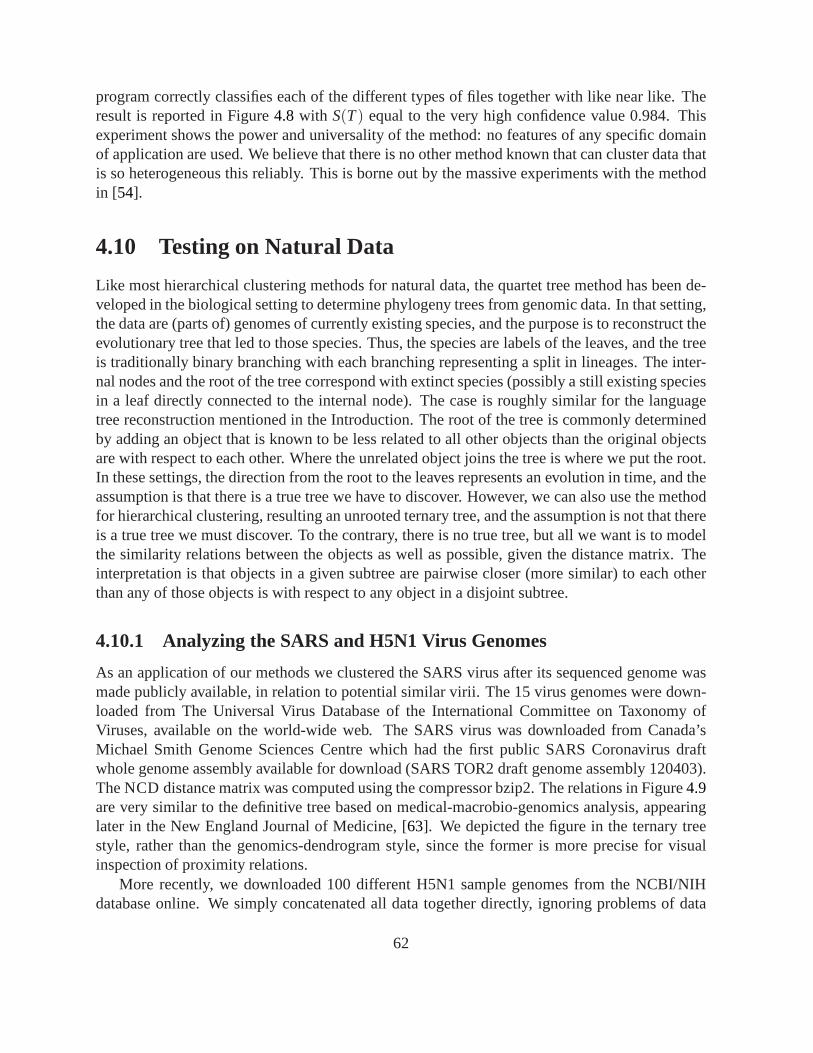
program correctly classifies each of the different types of files together with like near like. Theresult is reported in Figure4.8 with S(T) equal to the very high confidence value 0.984. Thisexperiment shows the power and universality of the method: no features of any specific domainof application are used. We believe that there is no other method known that can cluster data thatis so heterogeneous this reliably. This is borne out by the massive experiments with the methodin [54].
4.10 Testing on Natural Data
Like most hierarchical clustering methods for natural data, the quartet tree method has been de-veloped in the biological setting to determine phylogeny trees from genomic data. In that setting,the data are (parts of) genomes of currently existing species, and the purpose is to reconstruct theevolutionary tree that led to those species. Thus, the species are labels of the leaves, and the treeis traditionally binary branching with each branching representing a split in lineages. The inter-nal nodes and the root of the tree correspond with extinct species (possibly a still existing speciesin a leaf directly connected to the internal node). The case is roughly similar for the languagetree reconstruction mentioned in the Introduction. The root of the tree is commonly determinedby adding an object that is known to be less related to all other objects than the original objectsare with respect to each other. Where the unrelated object joins the tree is where we put the root.In these settings, the direction from the root to the leaves represents an evolution in time, and theassumption is that there is a true tree we have to discover. However, we can also use the methodfor hierarchical clustering, resulting an unrooted ternary tree, and the assumption is not that thereis a true tree we must discover. To the contrary, there is no true tree, but all we want is to modelthe similarity relations between the objects as well as possible, given the distance matrix. Theinterpretation is that objects in a given subtree are pairwise closer (more similar) to each otherthan any of those objects is with respect to any object in a disjoint subtree.
4.10.1 Analyzing the SARS and H5N1 Virus Genomes
As an application of our methods we clustered the SARS virus after its sequenced genome wasmade publicly available, in relation to potential similar virii. The 15 virus genomes were down-loaded from The Universal Virus Database of the International Committee on Taxonomy ofViruses, available on the world-wide web. The SARS virus wasdownloaded from Canada’sMichael Smith Genome Sciences Centre which had the first public SARS Coronavirus draftwhole genome assembly available for download (SARS TOR2 draft genome assembly 120403).The NCD distance matrix was computed using the compressor bzip2. The relations in Figure4.9are very similar to the definitive tree based on medical-macrobio-genomics analysis, appearinglater in the New England Journal of Medicine, [63]. We depicted the figure in the ternary treestyle, rather than the genomics-dendrogram style, since the former is more precise for visualinspection of proximity relations.
More recently, we downloaded 100 different H5N1 sample genomes from the NCBI/NIHdatabase online. We simply concatenated all data together directly, ignoring problems of data
62
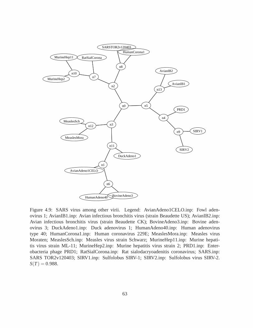
AvianAdeno1CELO
n1
n6
n11
AvianIB1
n13
n5
AvianIB2
BovineAdeno3HumanAdeno40
DuckAdeno1
n3
HumanCorona1
n8
SARSTOR2v120403
n2
MeaslesMora
n12MeaslesSch
MurineHep11
n10n7
MurineHep2
PRD1
n4
n9
RatSialCorona
SIRV1
SIRV2
n0
Figure 4.9: SARS virus among other virii. Legend: AvianAdeno1CELO.inp: Fowl aden-ovirus 1; AvianIB1.inp: Avian infectious bronchitis virus(strain Beaudette US); AvianIB2.inp:Avian infectious bronchitis virus (strain Beaudette CK); BovineAdeno3.inp: Bovine aden-ovirus 3; DuckAdeno1.inp: Duck adenovirus 1; HumanAdeno40.inp: Human adenovirustype 40; HumanCorona1.inp: Human coronavirus 229E; MeaslesMora.inp: Measles virusMoraten; MeaslesSch.inp: Measles virus strain Schwarz; MurineHep11.inp: Murine hepati-tis virus strain ML-11; MurineHep2.inp: Murine hepatitis virus strain 2; PRD1.inp: Enter-obacteria phage PRD1; RatSialCorona.inp: Rat sialodacryoadenitis coronavirus; SARS.inp:SARS TOR2v120403; SIRV1.inp: Sulfolobus SIRV-1; SIRV2.inp: Sulfolobus virus SIRV-2.S(T) = 0.988.
63
cleanup and duplication. We were warned in advance that certain coding regions in the viralgenome were sometimes listed twice and also many sequences are incomplete or missing certainproteins. In this case we sought to test the robustness at thehigh end and at the same timeverify, contextualize, and expand on the many claims of genetic similarity and diversity in thevirology community. We used the CompLearn package, [21], with theppmdcompressor for thisexperiment and performed no alignment step whatsoever. We used order 15 with 250 megabytesmemory maximum.
We have abbreviated Ck for Chicken and Dk for duck. Samples are named with species,location, sequence number, followed by the year double digits at the end. Naming is not 100%consistent. We can see the following features in Figure4.10, that are possibly significant:
First, there is near-perfect temporal separation by branchand year, going all the way backto HongKong and GuangDong in 1997. Next, there is near-perfect regional separation withclear delineation of Japan and the crucial Qinghai, Astrakhan, Mongolia, and Novosibirsk, aswell as near-perfect separation of Vietnam and Thailand. The placement CkVietnamC5804 andVietnam306204 is interesting in that they are both near Thailand branches and suggest that theymay be for example the migratory bird links that have been hypothesized or some other geneticintermediate. There is also throughout the tree substantial agreement with (and independent ver-ification of) independent experts like Dr. Henry L. Niman [86] on every specific point regardinggenetic similarity. The technique provides here an easy verification procedure without muchwork.
4.10.2 Music
The amount of digitized music available on the internet has grown dramatically in recent years,both in the public domain and on commercial sites. Napster and its clones are prime examples.Websites offering musical content in some form or other (MP3, MIDI, . . . ) need a way to or-ganize their wealth of material; they need to somehow classify their files according to musicalgenres and subgenres, putting similar pieces together. Thepurpose of such organization is toenable users to navigate to pieces of music they already knowand like, but also to give themadvice and recommendations (“If you like this, you might also like. . . ”). Currently, such orga-nization is mostly done manually by humans, but some recent research has been looking intothe possibilities of automating music classification. In [26, 25] we cluster music using the Com-pLearn Toolkit [21]. One example is a small set of classical piano sonatas, consisting of the 4movements from Debussy’s “Suite Bergamasque,” 4 movementsof book 2 of Bach’s “Wohltem-perierte Klavier,” and 4 preludes from Chopin’s “Opus 28.” As one can see in Figure4.11, ourprogram does a pretty good job at clustering these pieces. The S(T) score is also high: 0.968.The 4 Debussy movements form one cluster, as do the 4 Bach pieces. The only imperfection inthe tree, judged by what one would intuitively expect, is that Chopin’s Prélude no. 15 lies a bitcloser to Bach than to the other 3 Chopin pieces. This Préludeno 15, in fact, consistently formsan odd-one-out in our other experiments as well. This is an example of pure data mining, sincethere is some musical truth to this, as no. 15 is perceived as by far the most eccentric among the24 Préludes of Chopin’s opus 28.
64

Figure 4.10: One hundred H5N1 (bird flu) sample genomes, S(T)= 0.980221.
65
BachWTK2F1
BachWTK2F2
BachWTK2P1
BachWTK2P2
ChopPrel1
ChopPrel15
ChopPrel22
ChopPrel24
DebusBerg1
DebusBerg4
DebusBerg2
DebusBerg3
Figure 4.11: Output for the 12-piece set.
66
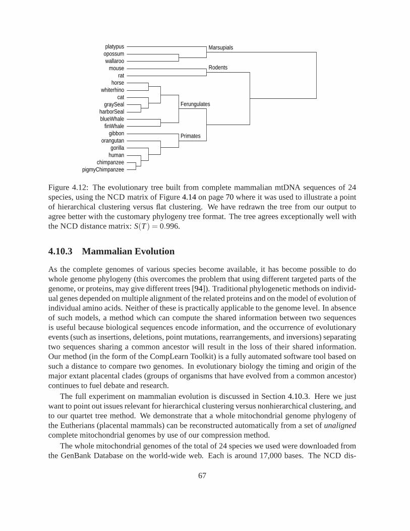
platypusopossumwallaroo
Marsupials
mouserat
Rodents
horsewhiterhino
catgraySeal
harborSealblueWhale
finWhale
Ferungulates
gibbonorangutan
gorillahuman
chimpanzeepigmyChimpanzee
Primates
Figure 4.12: The evolutionary tree built from complete mammalian mtDNA sequences of 24species, using the NCD matrix of Figure4.14on page70 where it was used to illustrate a pointof hierarchical clustering versus flat clustering. We have redrawn the tree from our output toagree better with the customary phylogeny tree format. The tree agrees exceptionally well withthe NCD distance matrix:S(T) = 0.996.
4.10.3 Mammalian Evolution
As the complete genomes of various species become available, it has become possible to dowhole genome phylogeny (this overcomes the problem that using different targeted parts of thegenome, or proteins, may give different trees [94]). Traditional phylogenetic methods on individ-ual genes depended on multiple alignment of the related proteins and on the model of evolution ofindividual amino acids. Neither of these is practically applicable to the genome level. In absenceof such models, a method which can compute the shared information between two sequencesis useful because biological sequences encode information, and the occurrence of evolutionaryevents (such as insertions, deletions, point mutations, rearrangements, and inversions) separatingtwo sequences sharing a common ancestor will result in the loss of their shared information.Our method (in the form of the CompLearn Toolkit) is a fully automated software tool based onsuch a distance to compare two genomes. In evolutionary biology the timing and origin of themajor extant placental clades (groups of organisms that have evolved from a common ancestor)continues to fuel debate and research.
The full experiment on mammalian evolution is discussed in Section4.10.3. Here we justwant to point out issues relevant for hierarchical clustering versus nonhierarchical clustering, andto our quartet tree method. We demonstrate that a whole mitochondrial genome phylogeny ofthe Eutherians (placental mammals) can be reconstructed automatically from a set ofunalignedcomplete mitochondrial genomes by use of our compression method.
The whole mitochondrial genomes of the total of 24 species weused were downloaded fromthe GenBank Database on the world-wide web. Each is around 17,000 bases. The NCD dis-
67
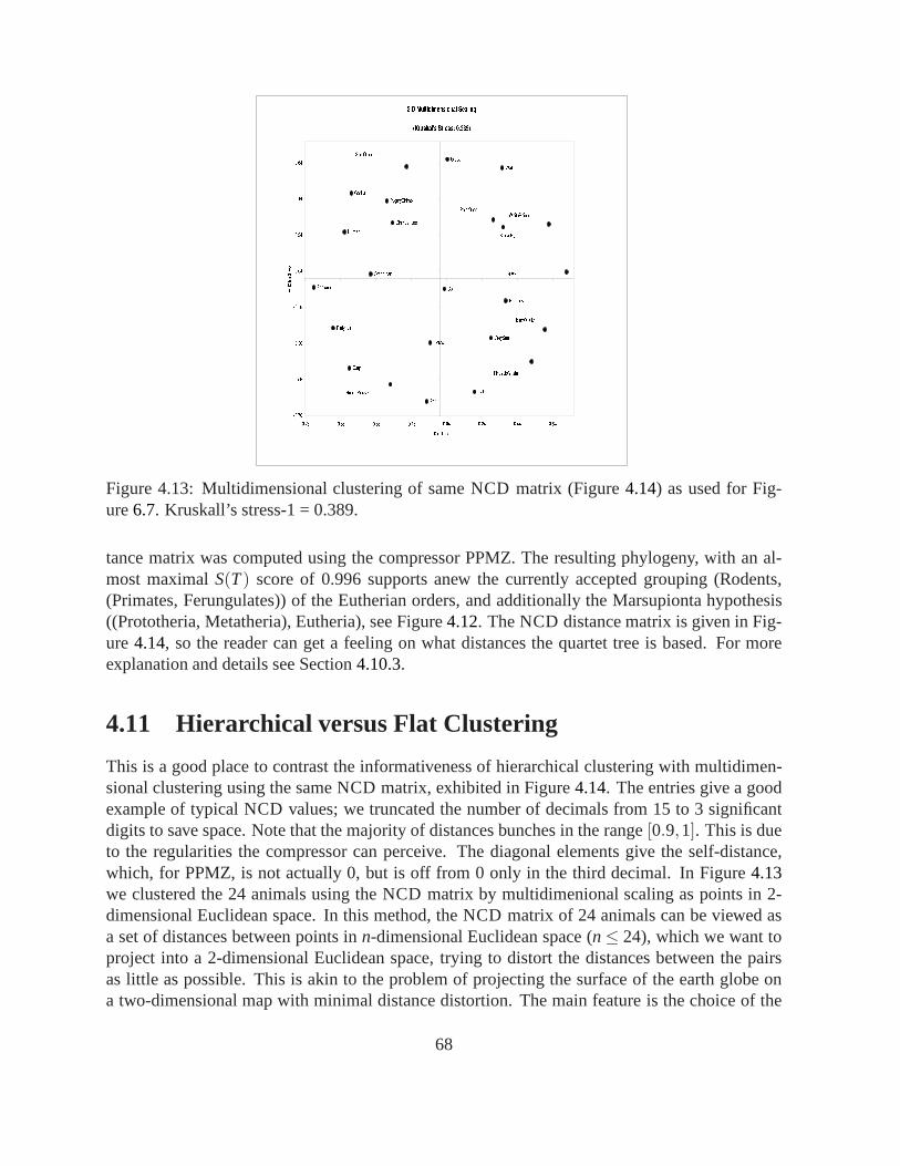
Figure 4.13: Multidimensional clustering of same NCD matrix (Figure4.14) as used for Fig-ure6.7. Kruskall’s stress-1 = 0.389.
tance matrix was computed using the compressor PPMZ. The resulting phylogeny, with an al-most maximalS(T) score of 0.996 supports anew the currently accepted grouping (Rodents,(Primates, Ferungulates)) of the Eutherian orders, and additionally the Marsupionta hypothesis((Prototheria, Metatheria), Eutheria), see Figure4.12. The NCD distance matrix is given in Fig-ure 4.14, so the reader can get a feeling on what distances the quartettree is based. For moreexplanation and details see Section4.10.3.
4.11 Hierarchical versus Flat Clustering
This is a good place to contrast the informativeness of hierarchical clustering with multidimen-sional clustering using the same NCD matrix, exhibited in Figure4.14. The entries give a goodexample of typical NCD values; we truncated the number of decimals from 15 to 3 significantdigits to save space. Note that the majority of distances bunches in the range[0.9,1]. This is dueto the regularities the compressor can perceive. The diagonal elements give the self-distance,which, for PPMZ, is not actually 0, but is off from 0 only in thethird decimal. In Figure4.13we clustered the 24 animals using the NCD matrix by multidimenional scaling as points in 2-dimensional Euclidean space. In this method, the NCD matrixof 24 animals can be viewed asa set of distances between points inn-dimensional Euclidean space (n≤ 24), which we want toproject into a 2-dimensional Euclidean space, trying to distort the distances between the pairsas little as possible. This is akin to the problem of projecting the surface of the earth globe ona two-dimensional map with minimal distance distortion. The main feature is the choice of the
68
measure of distortion to be minimized, [36]. Let the original set of distances bed1, . . . ,dk andthe projected distances bed′1, . . . ,d
′k. In Figure4.13we used the distortion measureKruskall’s
stress-1, [62], which minimizes√
(∑i≤k(di−d′i )2)/∑i≤k d2
i . Kruskall’s stress-1 equal 0 meansno distortion, and the worst value is at most 1 (unless you have a really bad projection). In theprojection of the NCD matrix according to our quartet methodone minimizes the more subtledistortionS(T) measure, where 1 means perfect representation of the relative relations betweenevery 4-tuple, and 0 means minimal representation. Therefore, we should compare distortionKruskall stress-1 with 1−S(T). Figure4.12has a very good 1−S(T) = 0.04 and Figure4.13has a poor Kruskall stress 0.389. Assuming that the comparison is significant for small val-ues (close to perfect projection), we find that the multidimensional scaling of this experiment’sNCD matrix is formally inferior to that of the quartet tree. This conclusion formally justifies theimpression conveyed by the figures on visual inspection.
69

Figure 4.14: Distance matrix of pairwise NCD. For display purpose, we have truncated theoriginal entries from 15 decimals to 3 decimals precision.
70
Chapter 5
Classification systems using NCD
This chapter explores the concept ofclassification. In rough terms, classification refers to theplacement of unknowntest objectsinto one of several categories based on a training set of ob-jects. It is different from the hierarchical clustering problem that has been the primary focusin this thesis up to this point, yet it is no less fundamental.Combining NCD with a trainablemachine learning module yields wonderfully effective and often surprising results, showing thatin certain situations, we may in essencelearn by examplewith the help of human experts. InSection5.1 below, classification is first addressed from a general perspective. In Section5.2,it is shown how to combine NCD in combination with trainable classifiers based on so-calledanchors. Section5.3 discusses two options for such trainable classifiers: neural networks andsupport vector machines.
5.1 Basic Classification
The classification problem setting as considered in this thesis is given as follows. A humanexpert has preparedn training examples. Each training example consists of ad-dimensionalinput vectorx and a target training labely. y must be chosen from a discrete setL of labels. Ahuman expert supplies this information; the accuracy of thetrained system would of course belimited by the accuracy of the labels in the training set. Atraining sessioncomputes a modelM from the input ortraining data(xi,yi) for 1≤ i ≤ n. The goal of a classification algorithmis to make good predictions based on the input training data.After M has been calculated bysomeclassifier learning algorithm, henceforth calledtrainable classifier system, it is used toclassify unknown test objectsxtest, also of dimensiond. It will output an element fromL foreach such object. Note thatM can be thought of as afunction that maps test input vectorsxto labels in the setL. We refer to such a function as aclassifier. Learning good classifiers isconsidered one of the most important problems in machine learning and pattern recognition incurrent times. One of the most important early successes hasbeen in the field of optical characterrecognition, or OCR. This is the problem of taking a rasterized bitmap image and converting it toa sequence of ASCII characters according to some symbol recognition algorithm. Typical OCRsoftware can work on as little as ten classes for applications such as numerical digit recognition,
71
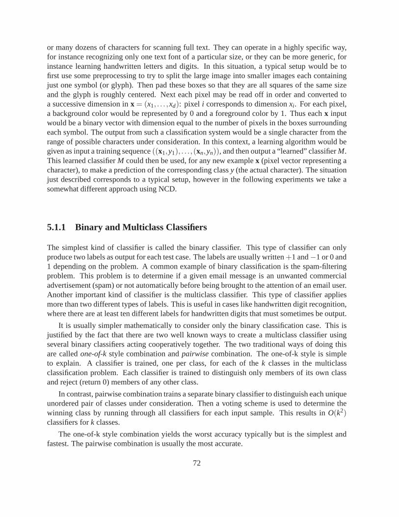
or many dozens of characters for scanning full text. They canoperate in a highly specific way,for instance recognizing only one text font of a particular size, or they can be more generic, forinstance learning handwritten letters and digits. In this situation, a typical setup would be tofirst use some preprocessing to try to split the large image into smaller images each containingjust one symbol (or glyph). Then pad these boxes so that they are all squares of the same sizeand the glyph is roughly centered. Next each pixel may be readoff in order and converted toa successive dimension inx = (x1, . . . ,xd): pixel i corresponds to dimensionxi . For each pixel,a background color would be represented by 0 and a foregroundcolor by 1. Thus eachx inputwould be a binary vector with dimension equal to the number ofpixels in the boxes surroundingeach symbol. The output from such a classification system would be a single character from therange of possible characters under consideration. In this context, a learning algorithm would begiven as input a training sequence((x1,y1), . . . ,(xn,yn)), and then output a “learned” classifierM.This learned classifierM could then be used, for any new examplex (pixel vector representing acharacter), to make a prediction of the corresponding classy (the actual character). The situationjust described corresponds to a typical setup, however in the following experiments we take asomewhat different approach using NCD.
5.1.1 Binary and Multiclass Classifiers
The simplest kind of classifier is called the binary classifier. This type of classifier can onlyproduce two labels as output for each test case. The labels are usually written+1 and−1 or 0 and1 depending on the problem. A common example of binary classification is the spam-filteringproblem. This problem is to determine if a given email message is an unwanted commercialadvertisement (spam) or not automatically before being brought to the attention of an email user.Another important kind of classifier is the multiclass classifier. This type of classifier appliesmore than two different types of labels. This is useful in cases like handwritten digit recognition,where there are at least ten different labels for handwritten digits that must sometimes be output.
It is usually simpler mathematically to consider only the binary classification case. This isjustified by the fact that there are two well known ways to create a multiclass classifier usingseveral binary classifiers acting cooperatively together.The two traditional ways of doing thisare calledone-of-kstyle combination andpairwisecombination. The one-of-k style is simpleto explain. A classifier is trained, one per class, for each ofthe k classes in the multiclassclassification problem. Each classifier is trained to distinguish only members of its own classand reject (return 0) members of any other class.
In contrast, pairwise combination trains a separate binaryclassifier to distinguish each uniqueunordered pair of classes under consideration. Then a voting scheme is used to determine thewinning class by running through all classifiers for each input sample. This results inO(k2)classifiers fork classes.
The one-of-k style combination yields the worst accuracy typically but is the simplest andfastest. The pairwise combination is usually the most accurate.
72
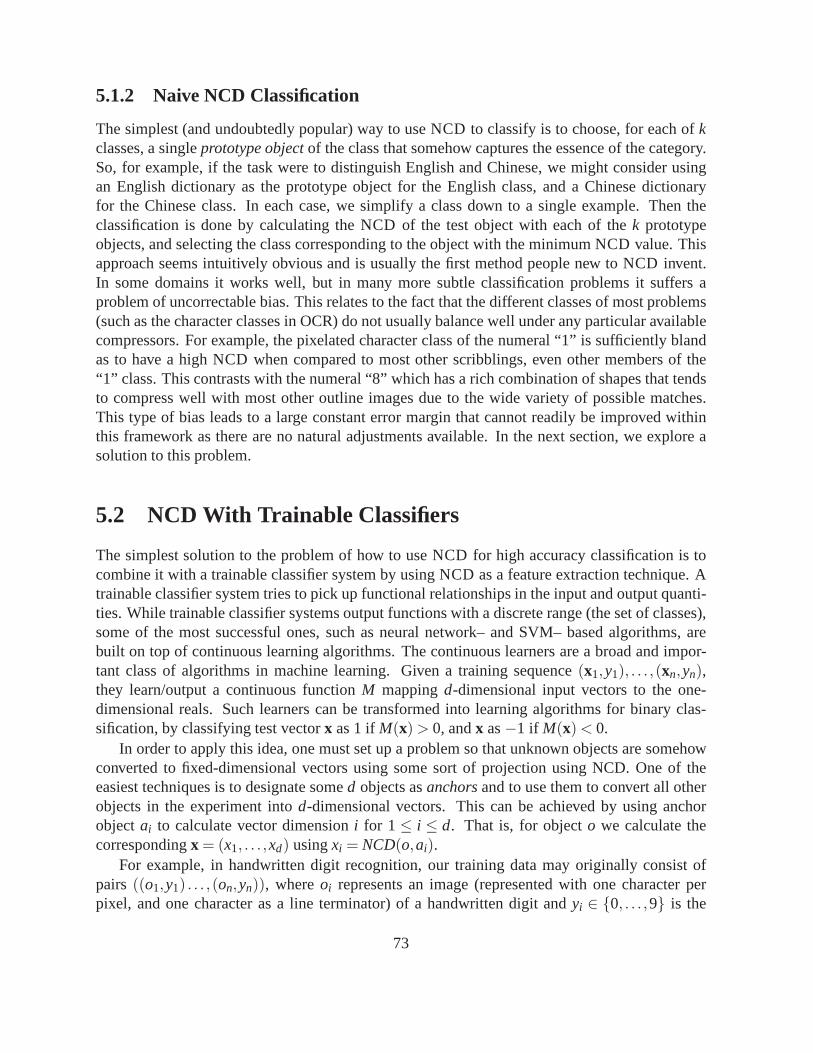
5.1.2 Naive NCD Classification
The simplest (and undoubtedly popular) way to use NCD to classify is to choose, for each ofkclasses, a singleprototype objectof the class that somehow captures the essence of the category.So, for example, if the task were to distinguish English and Chinese, we might consider usingan English dictionary as the prototype object for the English class, and a Chinese dictionaryfor the Chinese class. In each case, we simplify a class down to a single example. Then theclassification is done by calculating the NCD of the test object with each of thek prototypeobjects, and selecting the class corresponding to the object with the minimum NCD value. Thisapproach seems intuitively obvious and is usually the first method people new to NCD invent.In some domains it works well, but in many more subtle classification problems it suffers aproblem of uncorrectable bias. This relates to the fact thatthe different classes of most problems(such as the character classes in OCR) do not usually balancewell under any particular availablecompressors. For example, the pixelated character class ofthe numeral “1” is sufficiently blandas to have a high NCD when compared to most other scribblings,even other members of the“1” class. This contrasts with the numeral “8” which has a rich combination of shapes that tendsto compress well with most other outline images due to the wide variety of possible matches.This type of bias leads to a large constant error margin that cannot readily be improved withinthis framework as there are no natural adjustments available. In the next section, we explore asolution to this problem.
5.2 NCD With Trainable Classifiers
The simplest solution to the problem of how to use NCD for highaccuracy classification is tocombine it with a trainable classifier system by using NCD as afeature extraction technique. Atrainable classifier system tries to pick up functional relationships in the input and output quanti-ties. While trainable classifier systems output functions with a discrete range (the set of classes),some of the most successful ones, such as neural network– andSVM– based algorithms, arebuilt on top of continuous learning algorithms. The continuous learners are a broad and impor-tant class of algorithms in machine learning. Given a training sequence(x1,y1), . . . ,(xn,yn),they learn/output a continuous functionM mappingd-dimensional input vectors to the one-dimensional reals. Such learners can be transformed into learning algorithms for binary clas-sification, by classifying test vectorx as 1 ifM(x) > 0, andx as−1 if M(x) < 0.
In order to apply this idea, one must set up a problem so that unknown objects are somehowconverted to fixed-dimensional vectors using some sort of projection using NCD. One of theeasiest techniques is to designate somed objects asanchorsand to use them to convert all otherobjects in the experiment intod-dimensional vectors. This can be achieved by using anchorobjectai to calculate vector dimensioni for 1≤ i ≤ d. That is, for objecto we calculate thecorrespondingx = (x1, . . . ,xd) usingxi = NCD(o,ai).
For example, in handwritten digit recognition, our training data may originally consist ofpairs ((o1,y1) . . . ,(on,yn)), whereoi represents an image (represented with one character perpixel, and one character as a line terminator) of a handwritten digit andyi ∈ 0, . . . ,9 is the
73

corresponding digit. One then takes 80 imageso′1, . . . ,o′80, so that each handwritten digit is
represented eight times. The training data(o1, . . . ,on) are then converted to(x1, . . . ,xn), whereeachxi is the 80-dimensional vector(NCD(oi,o′1), . . . ,NCD(oi,o′80)).
5.2.1 Choosing Anchors
The anchors may be chosen by a human expert or be chosen randomly from a large pool of train-ing objects. Intuitively, it may seem very important which objects are chosen as anchors. Whilethis is sometimes the case, more often it is not. Random anchors usually work well. But mostpractitioners agree that picking at least one anchor from each significant category under consid-eration is advisable to avoid falling into low-accuracy performance due to insufficient variationin the anchor set. The anchor can be used with NCD. It can also be used with the NormalizedGoogle Distance (NGD), which we discuss in Chapter7. We will give details using NGD termsin Section7.6.4, and details using Optical Character Recognition with NCD in Section6.8.
In choosing a learning system to use with the anchor featuresextracted above, it seems bestto choose as general a learning system as possible. One particularly important class of learningalgorithms are called the universal continuous function learners. These include neural networksand Support Vector Machines. The universal learning property in this context means that theycan approximate any continuous function to an arbitrarily high degree of accuracy given enoughtraining data in the neighborhood of the point under consideration. Using a learner with thisproperty ensures a certain degree of reliability and optimality to the results that it generates ascompared to other more specialized learning algorithms.
5.3 Trainable Learners of Note
There are at least two good choices for trainable learner components for use with NCD. Theseare called theneural networkand theSupport Vector Machine. Both of these techniques take asinput the set of labeled training data as well as some specialized model parameters that must beset through some means. Usually the specialized parametersare set by a human expert or setthrough an automatic procedure using cross-validation based parameter scanning [11].
Both learner systems produce a single label out of the setL as a result given any inputd-dimensional test vector. Each have many strengths and weaknesses, and they each give uniqueperformance profiles. They should both be considered when deciding to do classification usingNCD, although all experiments in this thesis are based on support vector machines.
5.3.1 Neural Networks
The older and considerably popular choice is artificial neural networks [46]. As mentionedpreviously, these have the advantage of being universal classifier systems: they have provablelearning capability for any continuous function. Additionally, they have a host of decent trainingalgorithms as well as learning modes. Popular choices here are Fast Backpropagation and SelfOrganizing Maps. SOM’s have not been designed explicitly for classification, but can easily
74

adapted to be used for classification tasks when used in combination with compression metricslike NCD.
There is one major difficulty in all types of neural network investigated; they have somerather tricky parameter settings. A neural network of any sophistication must have a nonlinearcomponent (transfer function) of some sort, and common choices are transcendental sigmoidfunctions like arctangent. There are several others in use.Another hard issue with many typesof neural networks is to decide how many layers should be used. For each layer a specificnumber of neurons must be set in advance as well. Similarly, there is usually a learning rate andsometimes a momentum parameter that can radically affect the network’s gross behavior andoverall success or failure. Altogether this implies at least four hard choices before one can traina neural network. There is no simple rule to guide how to choose these parameters because thereare all sorts of bad behavior possible from wrong choices. The most common are overlearningand underlearning. Informally, overlearning occurs when there are too many neurons for the taskat hand. Underlearning is when there are too few. In the case of overlearning, the neural networkwill appear to have great accuracy in the training data yet terrible accuracy in the testing phaseand show almost no generalization capability. In the underlearning case, accuracy will simplybe capped at a number far worse than what may otherwise be achieved. It’s quite difficult to tellwhat the best parameters are for a neural network and in real commercial systems there is usuallya considerable amount of sophisticated semi-automatic machinery in place to assist the user insetting these parameters. For example, genetic algorithmsare sometimes employed combinedwith cross-validation to adjust parameters in a semi-automatic fashion. This heavy emphasis onparameter-setting in advance makes neural networks a difficult component to integrate into aneasy-to-use parameter-free learning system.
5.3.2 Support Vector Machines
More recently another type of continuous universal learnerhas come into great popularity. Theyhave the same sort of universal properties as artificial neural networks but with substantiallyless hassle [11]. They are called support vector machines. They take advantage of dot productsin a high dimensional space to efficiently find solutions to a convex optimization problem thatwinds up bending a decision surface around training points in the least stressful way. In orderto use an SVM, one needs to first choose a kernel function and this corresponds roughly to thetransfer function in neural networks. Although a linear kernel is an option and polynomials aresometimes used, they do not yield the same (typically desirable) infinite-dimensional propertiesthat the exponential Radial Basis Function kernels do. These are described further below.
For all of our experiments we have found RBF kernels to be about as good as any other choiceand often substantially better. There are only two other parameters for SVM’s. In our context,these are calledC andg. C is the cost for wrong answers, or training points that fall onthe wrongside of the decision boundary. Adjusting this can compensate for noisy or mislabeled trainingdata. Theg parameter represents kernel width and determines the rate of exponential decayaround each of the training points. The very wonderful property of both of these parameters isthat they can be determined through a simple two dimensionalgrid search.
This procedure was found to be much simpler to automate and far more robust than neural
75
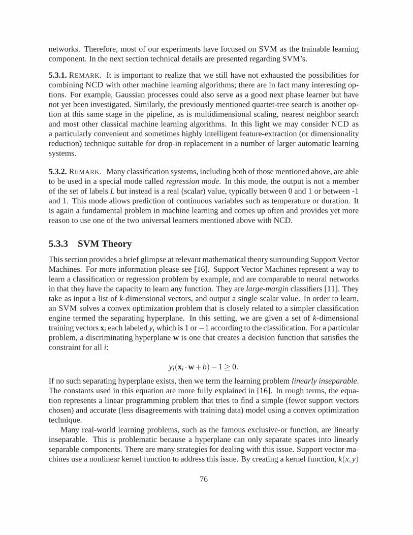
networks. Therefore, most of our experiments have focused on SVM as the trainable learningcomponent. In the next section technical details are presented regarding SVM’s.
5.3.1.REMARK . It is important to realize that we still have not exhausted the possibilities forcombining NCD with other machine learning algorithms; there are in fact many interesting op-tions. For example, Gaussian processes could also serve as agood next phase learner but havenot yet been investigated. Similarly, the previously mentioned quartet-tree search is another op-tion at this same stage in the pipeline, as is multidimensional scaling, nearest neighbor searchand most other classical machine learning algorithms. In this light we may consider NCD asa particularly convenient and sometimes highly intelligent feature-extraction (or dimensionalityreduction) technique suitable for drop-in replacement in anumber of larger automatic learningsystems.
5.3.2.REMARK . Many classification systems, including both of those mentioned above, are ableto be used in a special mode calledregression mode. In this mode, the output is not a memberof the set of labelsL but instead is a real (scalar) value, typically between 0 and1 or between -1and 1. This mode allows prediction of continuous variables such as temperature or duration. Itis again a fundamental problem in machine learning and comesup often and provides yet morereason to use one of the two universal learners mentioned above with NCD.
5.3.3 SVM Theory
This section provides a brief glimpse at relevant mathematical theory surrounding Support VectorMachines. For more information please see [16]. Support Vector Machines represent a way tolearn a classification or regression problem by example, andare comparable to neural networksin that they have the capacity to learn any function. They arelarge-marginclassifiers [11]. Theytake as input a list ofk-dimensional vectors, and output a single scalar value. In order to learn,an SVM solves a convex optimization problem that is closely related to a simpler classificationengine termed the separating hyperplane. In this setting, we are given a set ofk-dimensionaltraining vectorsxi each labeledyi which is 1 or−1 according to the classification. For a particularproblem, a discriminating hyperplanew is one that creates a decision function that satisfies theconstraint for alli:
yi(xi ·w+b)−1≥ 0.
If no such separating hyperplane exists, then we term the learning problemlinearly inseparable.The constants used in this equation are more fully explainedin [16]. In rough terms, the equa-tion represents a linear programming problem that tries to find a simple (fewer support vectorschosen) and accurate (less disagreements with training data) model using a convex optimizationtechnique.
Many real-world learning problems, such as the famous exclusive-or function, are linearlyinseparable. This is problematic because a hyperplane can only separate spaces into linearlyseparable components. There are many strategies for dealing with this issue. Support vector ma-chines use a nonlinear kernel function to address this issue. By creating a kernel function,k(x,y)
76

that satisfies theMercer condition, we may substantially enhance the power of the separatinghyperplane. A kernel function defines an inner-product on the input space, and then this innerproduct may be used to calculate many higher-power terms of combinations of samples in theinput space. This forms a higher-dimensional space, and it is well-known that once this space ismade large enough, there will be a separating hyperplane. Inour SVM experiments, we use aRadial Basis Function (RBF) kernel. This allows the SVM to learn any function given enoughtraining data.
5.3.4 SVM Parameter Setting
There are two parameters that control the learning of the SVM. The first relates to the kernelfunction. An RBF, or Radial Basis Function, kernel assumes the value 1 whenever the two inputvectors are equal. If they are unequal, it decays slowly towards 0 in a radially symmetric way:
K(xi ,x j) = e−‖xi−x j‖2/2g2.
Here,g is a parameter that controls the rate of decay or width of the kernel function. Because ofthe exponential form, the effective dimension of an RBF kernel is potentially infinite and thus thiskernel can be used to approximate any continuous function toan arbitrary degree of accuracy.This parameter must be set before the learning can begin withan SVM. Another parameterrelates to how misclassified points are handled in the training data; Though it is always possibleto simply continue to make the kernel width smaller and the expanded space larger until the SVMbecomes essentially a lookup-table, this is often not the best strategy for learning. An alternativeis to define a cost parameter and allow this to adjust the tolerance for misclassified points in thetraining data. This allows the SVM to generalize well even inthe presence of noisy data. Thiscost parameter, often calledc, must also be defined before training can begin.
We selectg and c using a grid searching technique. For each of these parameters, it isappropriate to search dozens of powers of two. Together, this creates a grid with hundreds ofdifferent parameter settings. We use five-fold cross-validation to select which of these grid pointsdefines the optimal parameter setting. First the data is divided into five random partitions: A, B,C, D, E. Then, for each candidate parameter setting or grid point, we run five different trainingruns. On the first run, we train on B, C, D, and E, and then we determine an accuracy using partA. Next, we train on A, C, D, E and test with B. We continue in this way and then average all fivetest scores to arrive at an estimate of how well the learning process performed. Once this processis done for all training data, we may just choose one of the grid points that attains a maximumaccuracy.
These parameters (C andg) do not usually need to be exact; instead one can simply do astepwise search along a grid of points in log space; thus it isfine to try just 64 points forC rangingfrom 2−31 to 232 doubling each time. A similar procedure works to chooseg. In each case onemay use five-fold cross-validation to estimate the accuracyof the given parameter setting andthen just choose the maximum at the end. Five-fold cross validation is a popular procedure thattries to estimate how well a model (of any type) that is trained on a set of training data willperform on unknown testing data. The basic assumption is simply that the training data and the
77

testing data are similar. In order to estimate the testing accuracy using only the training algorithmand the training data, first label the training set randomly with five labels, numbered 1 through 5.Next, train a model (SVM, neural network, or otherwise) on four of the five parts, but leave part 1out. Use this part 1 for testing the model made from the other 4parts. Tally this score and repeatthe procedure, but this time withhold part 2 for testing. Repeat this procedure five times, oncefor each part, and then average the accuracy scores to arriveat an estimate of the testing accuracyto be expected for a given set of parameters. This entire five-fold cross-validation procedure isrepeated for each point (particular parameter setting) in the parameter grid space in order to findthe optimal settings using just the training data.
78

Chapter 6
Experiments with NCD
This chapter demonstrates the surprisingly general and robust nature of the methods so far dis-cussed through many real examples from diverse areas such asmusic and evolution. The combi-nation of NCD and the quartet method yield interesting results.
In Section6.1, we introduce the general concept of feature-based similarity, and explain howNCD can be used with it. In Section6.2 we present experimental validation that our methodworks. Starting in Section6.4, we introduce a plethora of experiments in a wide array of fields,beginning with automatic music analysis. Next, we study evolutionary genomics, literature andlanguage analysis, radio astronomy, and optical characterrecognition. At the end of this chap-ter the reader will have encountered a highly serviceable survey of experimental results usingobjective data compressors based on files, without externalinformation input from the internet.
6.1 Similarity
We are presented with unknown data and the question is to determine the similarities amongthem and group like with like together. Commonly, the data are of a certain type: music files,transaction records of ATM machines, credit card applications, genomic data. In these data thereare hidden relations that we would like to get out in the open.For example, from genomic dataone can extract letter- or block frequencies (the blocks areover the four-letter alphabet); frommusic files one can extract various specific numerical features, related to pitch, rhythm, harmonyetc. One can extract such features using for instance Fourier transforms [114] or wavelet trans-forms [44]. The feature vectors corresponding to the various files arethen classified or clusteredusing existing classification software, based on various standard statistical pattern recognitionclassifiers [114], Bayesian classifiers [33], hidden Markov models [19], ensembles of nearestneighbor classifiers [44] or neural networks [33, 101]. For example, in music one feature wouldbe to look for rhythm in the sense of beats per minute. One can make a histogram where each his-togram bin corresponds to a particular tempo in beats-per-minute and the associated peak showshow frequent and strong that particular periodicity was over the entire piece. In [114] we seea gradual change from a few high peaks to many low and spread-out ones going from hip-hip,rock, jazz, to classical. One can use this similarity type totry to cluster pieces in these categories.
79
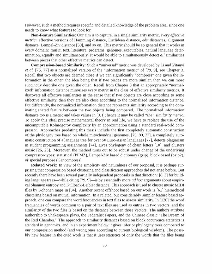
However, such a method requires specific and detailed knowledge of the problem area, since oneneeds to know what features to look for.
Non-Feature Similarities: Our aim is to capture, in a single similarity metric,every effectivemetric: effective versions of Hamming distance, Euclidean distance, edit distances, alignmentdistance, Lempel-Ziv distance [30], and so on. This metric should be so general that it works inevery domain: music, text, literature, programs, genomes,executables, natural language deter-mination, equally and simultaneously. It would be able to simultaneously detectall similaritiesbetween pieces that other effective metrics can detect.
Compression-based Similarity:Such a “universal” metric was developed by Li and Vitanyiet al. [75, 77] as a normalized version of the “information metric” of [79, 9], see Chapter 3.Recall that two objects are deemed close if we can significantly “compress” one given the in-formation in the other, the idea being that if two pieces are more similar, then we can moresuccinctly describe one given the other. Recall from Chapter 3 that an appropriately “normal-ized” information distance minorizes every metric in the class of effective similarity metrics. Itdiscovers all effective similarities in the sense that if two objects are close according to someeffective similarity, then they are also close according tothe normalized information distance.Put differently, the normalized information distance represents similarity according to the dom-inating shared feature between the two objects being compared. The normalized informationdistance too is a metric and takes values in[0,1]; hence it may be called“the” similarity metric.To apply this ideal precise mathematical theory in real life, we have to replace the use of theuncomputable Kolmogorov complexity by an approximation using a standard real-world com-pressor. Approaches predating this thesis include the firstcompletely automatic constructionof the phylogeny tree based on whole mitochondrial genomes,[75, 80, 77], a completely auto-matic construction of a language tree for over 50 Euro-Asianlanguages [77], detects plagiarismin student programming assignments [74], gives phylogeny of chain letters [10], and clustersmusic [26, 25]. Moreover, the method turns out to be robust under change ofthe underlyingcompressor-types: statistical (PPMZ), Lempel-Ziv based dictionary (gzip), block based (bzip2),or special purpose (Gencompress).
Related Work: In view of the simplicity and naturalness of our proposal, itis perhaps sur-prising that compression based clustering and classification approaches did not arise before. Butrecently there have been several partially independent proposals in that direction: [8, 3] for build-ing language trees—while citing [79, 9]—is by essentially moread hocarguments about empiri-cal Shannon entropy and Kullback-Leibler distance. This approach is used to cluster music MIDIfiles by Kohonen maps in [34]. Another recent offshoot based on our work is [61] hierarchicalclustering based on mutual information. In a related, but considerably simpler feature based ap-proach, one can compare the word frequencies in text files to assess similarity. In [120] the wordfrequencies of words common to a pair of text files are used as entries in two vectors, and thesimilarity of the two files is based on the distance between those vectors. The authors attributeauthorship to Shakespeare plays, the Federalist Papers, and the Chinese classic “The Dream ofthe Red Chamber.” The approach to similarity distances based on block occurrence statistics isstandard in genomics, and in an experiment below it gives inferior phylogeny trees compared toour compression method (and wrong ones according to currentbiological wisdom). The possi-bly new feature in the cited work is that it uses statistics ofonly the words that the files being
80
compared have in common. A related, opposite, approach was taken in [59], where literary textsare clustered by author gender or fact versus fiction, essentially by first identifying distinguishingfeatures, like gender dependent word usage, and then classifying according to those features.
Apart from the experiments reported here, the clustering bycompression method reportedin this thesis has recently been used to analyze network traffic and cluster computer worms andviruses [118]. Finally, recent work [54] reports experiments with our method on all time se-quence data used in all the major data-mining conferences inthe last decade. Comparing thecompression method with all major methods used in those conferences they established clear su-periority of the compression method for clustering heterogenous data, and for anomaly detection.
To substantiate our claim of universality, we apply the method to different areas, not usingany feature analysis at all. We first give an example in whole-genome phylogeny using thewhole mitochondrial DNA of the species concerned. We compare the hierarchical clusteringof our method with a more standard method of two-dimensionalclustering (to show that ourdendrogram method of depicting the clusters is more informative). We give a whole-genomephylogeny of fungi and compare this to results using alignment of selected proteins (alignmentbeing often too costly to perform on the whole-mitochondrial genome, but the disadvantage ofprotein selection being that different selections usuallyresult in different phylogenies—so whichis right?). We identify the virii that are closest to the sequenced SARS virus; we give an exampleof clustering of language families; Russian authors in the original Russian, the same pieces inEnglish translation (clustering partially follows the translators); clustering of music in MIDIformat; clustering of handwritten digits used for optical character recognition; and clusteringof radio observations of a mysterious astronomical object,a microquasar of extremely complexvariability. In all these cases the method performs very well in the following sense: The methodyields the phylogeny of 24 species precisely according to biological wisdom. The probabilitythat it randomly would hit this one outcome, or anything reasonably close, is very small. Inclustering 36 music pieces taken equally many from pop, jazz, classic, so that 12-12-12 is thegrouping we understand is correct, we can identify convex clusters so that only six errors aremade. (That is, if three items get dislodged then six items get misplaced.) The probability thatthis happens by chance is extremely small. The reason why we think the method does somethingremarkable is concisely put by Laplace [70]:
“If we seek a cause wherever we perceive symmetry, it is not that we regard thesymmetrical event as less possible than the others, but, since this event ought to bethe effect of a regular cause or that of chance, the first of these suppositions is moreprobable than the second. On a table we see letters arranged in this orderC o n s ta n t i n o p l e, and we judge that this arrangement is not the result of chance,not because it is less possible than others, for if this word were not employed in anylanguage we would not suspect it came from any particular cause, but this wordbeing in use among us, it is incomparably more probable that some person has thusarranged the aforesaid letters than that this arrangement is due to chance.”
Materials and Methods: The data samples we used were obtained from standard data basesaccessible on the world-wide web, generated by ourselves, or obtained from research groups in
81
the field of investigation. We supply the details with each experiment. The method of process-ing the data was the same in all experiments. First, we preprocessed the data samples to bringthem in appropriate format: the genomic material over the four-letter alphabetA,T,G,C isrecoded in a four-letter alphabet; the music MIDI files are stripped of identifying informationsuch as composer and name of the music piece. Then, in all cases the data samples were com-pletely automatically processed by our CompLearn Toolkit,rather than as is usual in phylogeny,by using an eclectic set of software tools per experiment. Oblivious to the problem area con-cerned, simply using the distances according to the NCD below, the method described in thisthesis fully automatically classifies the objects concerned. The CompLearn Toolkit is a suite ofsimple utilities that one can use to apply compression techniques to the process of discoveringand learning patterns in completely different domains. In fact, this method is so general that it re-quires no background knowledge about any particular subject area. There are no domain-specificparameters to set, and only a handful of general settings.
The CompLearn Toolkit using NCD and not, say, alignment, cancope with full genomes andother large data files and thus comes up with a single distancematrix. The clustering heuristicgenerates a tree with a certain confidence, called standardized benefit score orS(T) value in thesequel. Generating trees from the same distance matrix manytimes resulted in the same tree oralmost the same tree, for all distance matrices we used, eventhough the heuristic is randomized.The differences that arose are apparently due to early or late termination with differentS(T) val-ues. This is a great difference with previous phylogeny methods, where because of computationallimitations one uses only parts of the genome, or certain proteins that are viewed as significant[55]. These are run through a tree reconstruction method like neighbor joining [99], maximumlikelihood, maximum evolution, maximum parsimony as in [55], or quartet hypercleaning [13],many times. The percentage-wise agreement on certain branches arising are called “bootstrapvalues.” Trees are depicted with the best bootstrap values on the branches that are viewed assupporting the theory tested. Different choices of proteins result in different best trees. One wayto avoid this ambiguity is to use the full genome, [94, 77], leading to whole-genome phylogeny.With our method we do whole-genome phylogeny, and end up witha single overall best tree, notoptimizing selected parts of it.
The quality of the results depends on (a) the NCD distance matrix, and (b) how well thehierarchical tree represents the information in the matrix. The quality of (b) is measured bythe S(T) value, and is given with each experiment. In general, theS(T) value deteriorates forlarge sets. We believe this to be partially an artifact of a low-resolution NCD matrix due tolimited compression power, and limited file size. The main reason, however, is the fact that withincreasing size of a natural data set the projection of the information in the NCD matrix into abinary tree can get increasingly distorted as explained in Chapter 5, page45. Another aspectlimiting the quality of the NCD matrix is more subtle. Recallthat the method knows nothingabout any of the areas we apply it to. It determines the dominant feature as seen through theNCD filter. The dominant feature of likeness between two filesmay not correspond to our apriori conception but may have an unexpected cause. The results of our experiments suggest thatthis is not often the case: In the natural data sets where we have preconceptions of the outcome,for example that works by the same authors should cluster together, or music pieces by thesame composers, musical genres, or genomes, the outcomes conform largely to our expectations.
82
For example, in the music genre experiment the method would fail dramatically if genres wereevenly mixed, or mixed with little bias. However, to the contrary, the separation in clusters isalmost perfect. The few misplacements that are discernibleare either errors (the method wasnot powerful enough to discern the dominant feature), or thedominant feature between a pair ofmusic pieces is not the genre but some other aspect. The surprising news is that we can generallyconfirm expectations with few misplacements, indeed, that the data does not contain unknownrogue features that dominate to cause spurious (in our preconceived idea) clustering. This givesevidence that where the preconception is in doubt, like withphylogeny hypotheses, the clusteringcan give true support of one hypothesis against another one.
Figures: We use two styles to display the hierarchical clusters. In the case of genomics ofEutherian orders and fungi, language trees, it is convenient to follow the dendrograms that arecustomary in that area (suggesting temporal evolution) foreasy comparison with the literature.Although there is no temporal relation intended, the dendrogram representation looked also ap-propriate for the Russian writers, and translations of Russian writers. In the other experiments(even the genomic SARS experiment) it is more informative todisplay an unrooted ternary tree(or binary tree if we think about incoming and outgoing edges) with explicit internal nodes. Thisfacilitates identification of clusters in terms of subtreesrooted at internal nodes or contiguoussets of subtrees rooted at branches of internal nodes.
Testing the similarity machine on natural data: We test gross classification of files basedon markedly different file types. Here, we chose several files: (i) Four mitochondrial gene se-quences, from a black bear, polar bear, fox, and rat obtainedfrom the GenBank Database onthe world-wide web; (ii) Four excerpts from the novelThe Zeppelin’s Passengerby E. PhillipsOppenheim, obtained from the Project Gutenberg Edition on the World Wide web; (iii) FourMIDI files without further processing; two from Jimi Hendrixand two movements from De-bussy’s Suite Bergamasque, downloaded from various repositories on the world-wide web; (iv)Two Linux x86 ELF executables (thecpandrm commands), copied directly from the RedHat 9.0Linux distribution; and (v) Two compiled Java class files, generated by ourselves. The compres-sor used to compute the NCD matrix was bzip2. As expected, theprogram correctly classifieseach of the different types of files together with like near like. The result is reported in Figure6.1with S(T) equal to the very high confidence value 0.984. This experiment shows the power anduniversality of the method: no features of any specific domain of application are used.
6.2 Experimental Validation
We developed the CompLearn Toolkit, and performed experiments in vastly different applicationfields to test the quality and universality of the method. Thesuccess of the method as reportedbelow depends strongly on the judicious use of encoding of the objects compared. Here oneshould use common sense on what a real world compressor can do. There are situations whereour approach fails if applied in a straightforward way. For example: comparing text files bythe same authors in different encodings (say, Unicode and 8-bit version) is bound to fail. For theideal similarity metric based on Kolmogorov complexity as defined in [77] this does not matter atall, but for practical compressors used in the experiments it will be fatal. Similarly, in the music
83

experiments below we use symbolic MIDI music file format rather than wave format music files.The reason is that the strings resulting from straightforward discretizing the wave form files maybe too sensitive to how we discretize.
6.3 Truly Feature-Free: The Case of Heterogenous Data
ELFExecutableA
ELFExecutableB
GenesBlackBearA
GenesPolarBearB
GenesFoxC
GenesRatD
JavaClassA
JavaClassB
MusicBergA
MusicBergB
MusicHendrixA
MusicHendrixB
TextA
TextB
TextC
TextD
Figure 6.1: Classification of different file types. Tree agrees exceptionally well with NCD dis-tance matrix:S(T) = 0.984.
We show the method is truly feature-free, or, anyway, as feature-free as we could possiblywant, by showing once more its success in clustering data from truly different domains. No othermethod can apparently do so with so much success, since all other methods rfely on some definitefeatures they analyze. In contrast, we just compress. Onr may say that the used compressor de-termines the features analyzed, but this seems ill-tergeted at general-purpose compressors whichsimply aim at analyzing general features as well as is possible. We test gross classification offiles based on markedly different file types, as on page84, recalling Figure6.1displayed there.
1. Four mitochondrial gene sequences, from a black bear, polar bear, fox, and rat.
2. Four excerpts from the novelThe Zeppelin’s Passengerby E. Phillips Oppenheim
84
3. Four MIDI files without further processing; two from Jimi Hendrix and two movementsfrom Debussy’s Suite bergamasque
4. Two Linux x86 ELF executables (thecp andrm commands)
5. Two compiled Java class files.
As expected, the program correctly classifies each of the different types of files together with likenear like. The result is reported in Figure6.1with S(T) equal to 0.984. Recall thatS is definedas a linear normalized and inverted tree cost score as previously explained in Chapter 5, page49.This means that this tree is very near an optimal best tree.
6.4 Music Categorization
The first result found relates to music analysis using gzip orbzip2 with preprocessed MIDI files.Surprisingly, the computer was able to reconstruct some common musical notions without anytraining whatsoever using just compression and quartet tree search.
A human expert, comparing different pieces of music with theaim to cluster likes together,will generally look for certain specific similarities. Previous attempts to automate this processdo the same. Generally speaking, they take a file containing apiece of music and extract fromit various specific numerical features, related to pitch, rhythm, harmony etc. One can extractsuch features using for instance Fourier transforms [114] or wavelet transforms [44]. The featurevectors corresponding to the various files are then classified or clustered using existing classifica-tion software, based on various standard statistical pattern recognition classifiers [114], Bayesianclassifiers [33], hidden Markov models [19], ensembles of nearest-neighbor classifiers [44] orneural networks [33, 101]. For example, one feature would be to look for rhythm in the senseof beats per minute. One can make a histogram where each histogram bin corresponds to a par-ticular tempo in beats-per-minute and the associated peak shows how frequent and strong thatparticular periodicity was over the entire piece. In [114] we see a gradual change from a few highpeaks to many low and spread-out ones going from hip-hip, rock, jazz, to classical. One can usethis similarity type to try to cluster pieces in these categories. However, such a method requiresspecific and detailed knowledge of the problem area, since one needs to know what features tolook for.
Our aim is much more general. We do not look for similarity in specific features known tobe relevant for classifying music; instead we apply a general mathematical theory of similarity.The aim is to capture, in a single similarity metric,every effective metric: effective versions ofHamming distance, Euclidean distance, edit distances, Lempel-Ziv distance, and so on. Such ametric would be able to simultaneously detectall similarities between pieces that other effectivemetrics can detect. As we have seen in Chapter 3, such a “universal” metric indeed exists. It isthe NID metric which is approximated by the NCD metric.
In this section we apply this compression-based method to the classification of pieces of mu-sic. We perform various experiments on sets of mostly classical pieces given as MIDI (MusicalInstrument Digital Interface) files. This contrasts with most earlier research, where the music
85
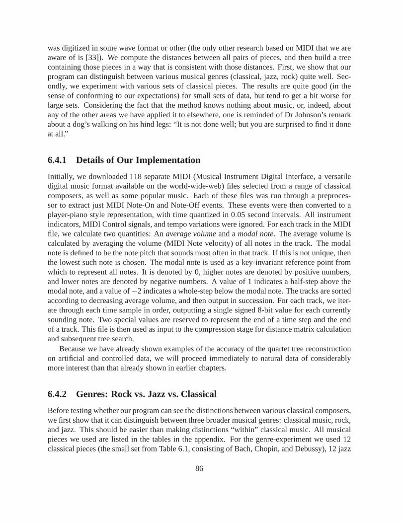
was digitized in some wave format or other (the only other research based on MIDI that we areaware of is [33]). We compute the distances between all pairs of pieces, andthen build a treecontaining those pieces in a way that is consistent with those distances. First, we show that ourprogram can distinguish between various musical genres (classical, jazz, rock) quite well. Sec-ondly, we experiment with various sets of classical pieces.The results are quite good (in thesense of conforming to our expectations) for small sets of data, but tend to get a bit worse forlarge sets. Considering the fact that the method knows nothing about music, or, indeed, aboutany of the other areas we have applied it to elsewhere, one is reminded of Dr Johnson’s remarkabout a dog’s walking on his hind legs: “It is not done well; but you are surprised to find it doneat all.”
6.4.1 Details of Our Implementation
Initially, we downloaded 118 separate MIDI (Musical Instrument Digital Interface, a versatiledigital music format available on the world-wide-web) filesselected from a range of classicalcomposers, as well as some popular music. Each of these files was run through a preproces-sor to extract just MIDI Note-On and Note-Off events. These events were then converted to aplayer-piano style representation, with time quantized in0.05 second intervals. All instrumentindicators, MIDI Control signals, and tempo variations were ignored. For each track in the MIDIfile, we calculate two quantities: Anaverage volumeand amodal note. The average volume iscalculated by averaging the volume (MIDI Note velocity) of all notes in the track. The modalnote is defined to be the note pitch that sounds most often in that track. If this is not unique, thenthe lowest such note is chosen. The modal note is used as a key-invariant reference point fromwhich to represent all notes. It is denoted by 0, higher notesare denoted by positive numbers,and lower notes are denoted by negative numbers. A value of 1 indicates a half-step above themodal note, and a value of−2 indicates a whole-step below the modal note. The tracks aresortedaccording to decreasing average volume, and then output in succession. For each track, we iter-ate through each time sample in order, outputting a single signed 8-bit value for each currentlysounding note. Two special values are reserved to representthe end of a time step and the endof a track. This file is then used as input to the compression stage for distance matrix calculationand subsequent tree search.
Because we have already shown examples of the accuracy of thequartet tree reconstructionon artificial and controlled data, we will proceed immediately to natural data of considerablymore interest than that already shown in earlier chapters.
6.4.2 Genres: Rock vs. Jazz vs. Classical
Before testing whether our program can see the distinctionsbetween various classical composers,we first show that it can distinguish between three broader musical genres: classical music, rock,and jazz. This should be easier than making distinctions “within” classical music. All musicalpieces we used are listed in the tables in the appendix. For the genre-experiment we used 12classical pieces (the small set from Table6.1, consisting of Bach, Chopin, and Debussy), 12 jazz
86

pieces (Table6.2), and 12 rock pieces (Table6.3). The tree that our program came up with isgiven in Figure6.2. TheS(T) score is 0.858.
BachWTK2F1
BachWTK2P2
BachWTK2F2
PoliceMess
BachWTK2P1
GershSumm
BeatlEleanor
ClaptonCoca
BeatlMich
MetalOne
ChopPrel1
ChopPrel22
ChopPrel15
ColtrLazybird
ChopPrel24
MilesSowhat
ClaptonLayla
PoliceBreath
ColtrBlueTr
MilesMilesto
ColtrGiantStp
DireStMoney
ColtrImpres
MilesSolar
DebusBerg1
DebusBerg4
DebusBerg2
DebusBerg3
GilleTunisia
Miles7steps
HendrixJoe
LedZStairw
HendrixVoodoo
RushYyz
MonkRoundM
ParkYardbird
Figure 6.2: Output for the 36 pieces from 3 genres.
The discrimination between the 3 genres is good but not perfect. The upper branch of the treecontains 10 of the 12 jazz pieces, but also Chopin’s Prélude no. 15 and a Bach Prelude. The twoother jazz pieces, Miles Davis’ “So what” and John Coltrane’s “Giant steps” are placed elsewherein the tree, perhaps according to some kinship that now escapes us but can be identified by closerstudying of the objects concerned. Of the rock pieces, 9 are placed close together in the rightmostbranch, while Hendrix’s “Voodoo chile”, Rush’ “Yyz”, and Dire Straits’ “Money for nothing”are further away. In the case of the Hendrix piece this may be explained by the fact that it doesnot fit well in a specific genre. Most of the classical pieces are in the lower left part of the tree.Surprisingly, 2 of the 4 Bach pieces are placed elsewhere. Itis not clear why this happens andmay be considered an error of our program, since we perceive the 4 Bach pieces to be very close,both structurally and melodically (as they all come from themono-thematic “WohltemperierteKlavier”). However, Bach’s is a seminal music and has been copied and cannibalized in all kindsof recognizable or hidden manners; closer scrutiny could reveal likenesses in its present company
87

BachWTK2F1
BachWTK2F2
BachWTK2P1
BachWTK2P2
ChopPrel1
ChopPrel15
ChopPrel22
ChopPrel24
DebusBerg1
DebusBerg4
DebusBerg2
DebusBerg3
Figure 6.3: Output for the 12-piece set.
that are not now apparent to us. In effect our similarity engine aims at the ideal of a perfect datamining process, discovering unknown features in which the data can be similar.
6.4.3 Classical Piano Music (Small Set)
In Table6.1 we list all 60 classical piano pieces used, together with their abbreviations. Someof these are complete compositions, others are individual movements from larger compositions.They all are piano pieces, but experiments on 34 movements ofsymphonies gave very similarresults (Section6.4.6). Apart from running our program on the whole set of 60 piano pieces,we also tried it on two smaller sets: a small 12-piece set, indicated by ‘(s)’ in the table, and amedium-size 32-piece set, indicated by ‘(s)’ or ‘(m)’.
The small set encompasses the 4 movements from Debussy’s Suite bergamasque, 4 move-ments of book 2 of Bach’s Wohltemperierte Klavier, and 4 preludes from Chopin’s opus 28. Asone can see in Figure6.3, our program does a pretty good job at clustering these pieces. TheS(T) score is also high: 0.958. The 4 Debussy movements form one cluster, as do the 4 Bachpieces. The only imperfection in the tree, judged by what onewould intuitively expect, is thatChopin’s Prélude no. 15 lies a bit closer to Bach than to the other 3 Chopin pieces. This Préludeno 15, in fact, consistently forms an odd-one-out in our other experiments as well. This is anexample of pure data mining, since there is some musical truth to this, as no. 15 is perceived as
88
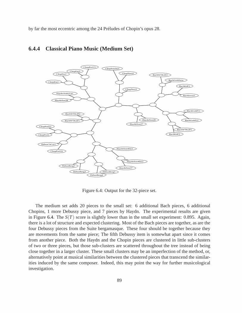
by far the most eccentric among the 24 Préludes of Chopin’s opus 28.
6.4.4 Classical Piano Music (Medium Set)
BachGoldAria
BachWTK2F2
BachGoldV1
BachGoldV2
BachInven1
BachKdF1
BachKdF2
BachWTK2P1
BachWTK2F1
BachWTK2P2
ChopEtu1
ChopEtu2
ChopEtu3
ChopPrel15
ChopNoct1
ChopNoct2
ChopSon2m3
ChopPrel1
ChopPrel22
ChopPrel24
DebusChCor1
DebusBerg1
DebusBerg4
DebusBerg2
DebusBerg3
HaydnAndaVari
HaydnSon38
HaydnSon27
HaydnSon28
HaydnSon37
HaydnSon40m2
HaydnSon40m1
Figure 6.4: Output for the 32-piece set.
The medium set adds 20 pieces to the small set: 6 additional Bach pieces, 6 additionalChopins, 1 more Debussy piece, and 7 pieces by Haydn. The experimental results are givenin Figure6.4. TheS(T) score is slightly lower than in the small set experiment: 0.895. Again,there is a lot of structure and expected clustering. Most of the Bach pieces are together, as are thefour Debussy pieces from the Suite bergamasque. These four should be together because theyare movements from the same piece; The fifth Debussy item is somewhat apart since it comesfrom another piece. Both the Haydn and the Chopin pieces are clustered in little sub-clustersof two or three pieces, but those sub-clusters are scatteredthroughout the tree instead of beingclose together in a larger cluster. These small clusters maybe an imperfection of the method, or,alternatively point at musical similarities between the clustered pieces that transcend the similar-ities induced by the same composer. Indeed, this may point the way for further musicologicalinvestigation.
89
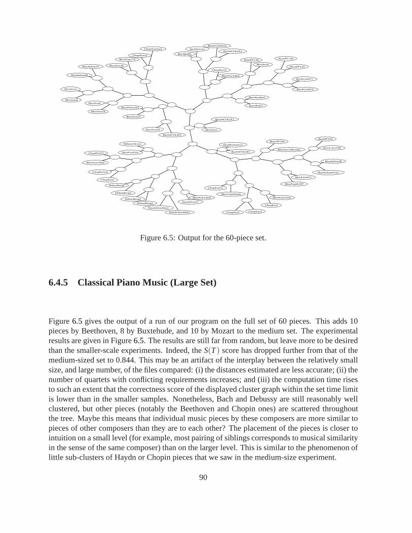
BachGoldAria
BachWTK2F2
BachGoldV1
BachGoldV2
BachInven1
BachKdF1
BachKdF2
BeetSon8m1
BachWTK2F1
MozSon1
BachWTK2P1
BeetSon29
BachWTK2P2
BeetRomance1
BeetFurElise
DebusChCor1
BeetSon14m1
ChopNoct1
BeetSon14m2
ChopPrel22
BeetSon14m3
HaydnSon37
BeetSon21m2
ChopEtu1
BeetSon23
BuxtPassa161
BeetSon26
BuxtFug174
BuxtCanz168
BuxtPF163
BuxtPF139
MozSon2
BuxtPF143
BuxtPF144
BuxtTF165
MozSon16Rondo
ChopEtu2
ChopEtu3
ChopNoct2
ChopSon2m3
ChopPrel1
ChopPrel24
ChopPrel15
MozVarsDirais
DebusBerg1
DebusBerg4
DebusBerg2
DebusBerg3
HaydnAndaVari
HaydnSon38
HaydnSon27
HaydnSon28
HaydnSon40m1
HaydnSon40m2
MozFant475
MozFantK397
MozSon19
MozSon6
MozSon3
MozSon4
Figure 6.5: Output for the 60-piece set.
6.4.5 Classical Piano Music (Large Set)
Figure6.5 gives the output of a run of our program on the full set of 60 pieces. This adds 10pieces by Beethoven, 8 by Buxtehude, and 10 by Mozart to the medium set. The experimentalresults are given in Figure6.5. The results are still far from random, but leave more to be desiredthan the smaller-scale experiments. Indeed, theS(T) score has dropped further from that of themedium-sized set to 0.844. This may be an artifact of the interplay between the relatively smallsize, and large number, of the files compared: (i) the distances estimated are less accurate; (ii) thenumber of quartets with conflicting requirements increases; and (iii) the computation time risesto such an extent that the correctness score of the displayedcluster graph within the set time limitis lower than in the smaller samples. Nonetheless, Bach and Debussy are still reasonably wellclustered, but other pieces (notably the Beethoven and Chopin ones) are scattered throughoutthe tree. Maybe this means that individual music pieces by these composers are more similar topieces of other composers than they are to each other? The placement of the pieces is closer tointuition on a small level (for example, most pairing of siblings corresponds to musical similarityin the sense of the same composer) than on the larger level. This is similar to the phenomenon oflittle sub-clusters of Haydn or Chopin pieces that we saw in the medium-size experiment.
90
BeetSym3m1
BeetSym3m4
BeetSym3m2
BeetSym5m1
BeetSym3m3
HaydnSym104m4
BeetSym4m1
MozSym39m3
BeetSym4m2
BeetSym5m2
BeetSym4m3
BeetSym5m3
BeetSym4m4
SSanSym3m2
BeetSym5m4
SchuSym8m1
HaydnSym104m1
SchuSym8m2
HaydnSym104m2
HaydnSym104m3
HaydnSym95
MozSym39m2
MozSym39m1
MozSym41m4
MozSym39m4
MozSym40m4
MozSym40m1
MozSym41m1
MozSym40m2
MozSym41m2
MozSym40m3
MozSym41m3
SSanSym3m1
SSanSym3m3
Figure 6.6: Output for the set of 34 movements of symphonies.
6.4.6 Clustering Symphonies
Finally, we tested whether the method worked for more complicated music, namely 34 sym-phonic pieces. We took two Haydn symphonies (no. 95 in one file, and the four movementsof 104), three Mozart symphonies (39, 40, 41), three Beethoven symphonies (3, 4, 5), of Schu-bert’s Unfinished symphony, and of Saint-Saens Symphony no.3. The results are reported inFigure6.6, with a quite reasonableS(T) score of 0.860.
6.4.7 Future Music Work and Conclusions
Our research raises many questions worth looking into further:
• The program can be used as a data mining machine to discover hitherto unknown simi-larities between music pieces of different composers or indeed different genres. In thismanner we can discover plagiarism or indeed honest influences between music pieces andcomposers. Indeed, it is thinkable that we can use the methodto discover seminality ofcomposers, or separate music eras and fads.
• A very interesting application of our program would be to select a plausible composer for anewly discovered piece of music of which the composer is not known. In addition to such
91
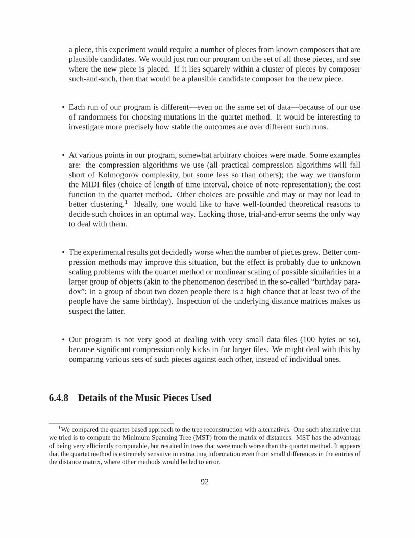
a piece, this experiment would require a number of pieces from known composers that areplausible candidates. We would just run our program on the set of all those pieces, and seewhere the new piece is placed. If it lies squarely within a cluster of pieces by composersuch-and-such, then that would be a plausible candidate composer for the new piece.
• Each run of our program is different—even on the same set of data—because of our useof randomness for choosing mutations in the quartet method.It would be interesting toinvestigate more precisely how stable the outcomes are overdifferent such runs.
• At various points in our program, somewhat arbitrary choices were made. Some examplesare: the compression algorithms we use (all practical compression algorithms will fallshort of Kolmogorov complexity, but some less so than others); the way we transformthe MIDI files (choice of length of time interval, choice of note-representation); the costfunction in the quartet method. Other choices are possible and may or may not lead tobetter clustering.1 Ideally, one would like to have well-founded theoretical reasons todecide such choices in an optimal way. Lacking those, trial-and-error seems the only wayto deal with them.
• The experimental results got decidedly worse when the number of pieces grew. Better com-pression methods may improve this situation, but the effectis probably due to unknownscaling problems with the quartet method or nonlinear scaling of possible similarities in alarger group of objects (akin to the phenomenon described inthe so-called “birthday para-dox”: in a group of about two dozen people there is a high chance that at least two of thepeople have the same birthday). Inspection of the underlying distance matrices makes ussuspect the latter.
• Our program is not very good at dealing with very small data files (100 bytes or so),because significant compression only kicks in for larger files. We might deal with this bycomparing various sets of such pieces against each other, instead of individual ones.
6.4.8 Details of the Music Pieces Used
1We compared the quartet-based approach to the tree reconstruction with alternatives. One such alternative thatwe tried is to compute the Minimum Spanning Tree (MST) from the matrix of distances. MST has the advantageof being very efficiently computable, but resulted in trees that were much worse than the quartet method. It appearsthat the quartet method is extremely sensitive in extracting information even from small differences in the entries ofthe distance matrix, where other methods would be led to error.
92
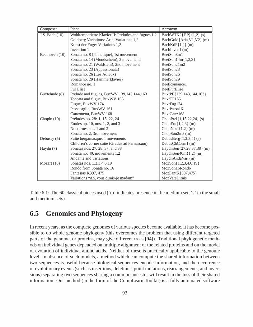
Composer Piece Acronym
J.S. Bach (10) Wohltemperierte Klavier II: Preludes and fugues 1,2BachWTK2F,P1,2 (s)Goldberg Variations: Aria, Variations 1,2 BachGoldAria,V1,V2 (m)Kunst der Fuge: Variations 1,2 BachKdF1,2 (m)Invention 1 BachInven1 (m)
Beethoven (10) Sonata no. 8 (Pathetique), 1st movement BeetSon8m1Sonata no. 14 (Mondschein), 3 movements BeetSon14m1,2,3Sonata no. 21 (Waldstein), 2nd movement BeetSon21m2Sonata no. 23 (Appassionata) BeetSon23Sonata no. 26 (Les Adieux) BeetSon26Sonata no. 29 (Hammerklavier) BeetSon29Romance no. 1 BeetRomance1Für Elise BeetFurElise
Buxtehude (8) Prelude and fugues, BuxWV 139,143,144,163 BuxtPF139,143,144,163Toccata and fugue, BuxWV 165 BuxtTF165Fugue, BuxWV 174 BuxtFug174Passacaglia, BuxWV 161 BuxtPassa161Canzonetta, BuxWV 168 BuxtCanz168
Chopin (10) Préludes op. 28: 1, 15, 22, 24 ChopPrel1,15,22,24 (s)Etudes op. 10, nos. 1, 2, and 3 ChopEtu1,2,3 (m)Nocturnes nos. 1 and 2 ChopNoct1,2 (m)Sonata no. 2, 3rd movement ChopSon2m3 (m)
Debussy (5) Suite bergamasque, 4 movements DebusBerg1,2,3,4 (s)Children’s corner suite (Gradus ad Parnassum) DebusChCorm1 (m)
Haydn (7) Sonatas nos. 27, 28, 37, and 38 HaydnSon27,28,37,38 (m)Sonata no. 40, movements 1,2 HaydnSon40m1,2 (m)Andante and variations HaydnAndaVari (m)
Mozart (10) Sonatas nos. 1,2,3,4,6,19 MozSon1,2,3,4,6,19Rondo from Sonata no. 16 MozSon16RondoFantasias K397, 475 MozFantK397,475Variations “Ah, vous dirais-je madam” MozVarsDirais
Table 6.1: The 60 classical pieces used (‘m’ indicates presence in the medium set, ‘s’ in the smalland medium sets).
6.5 Genomics and Phylogeny
In recent years, as the complete genomes of various species become available, it has become pos-sible to do whole genome phylogeny (this overcomes the problem that using different targetedparts of the genome, or proteins, may give different trees [94]). Traditional phylogenetic meth-ods on individual genes depended on multiple alignment of the related proteins and on the modelof evolution of individual amino acids. Neither of these is practically applicable to the genomelevel. In absence of such models, a method which can compute the shared information betweentwo sequences is useful because biological sequences encode information, and the occurrenceof evolutionary events (such as insertions, deletions, point mutations, rearrangements, and inver-sions) separating two sequences sharing a common ancestor will result in the loss of their sharedinformation. Our method (in the form of the CompLearn Toolkit) is a fully automated software
93
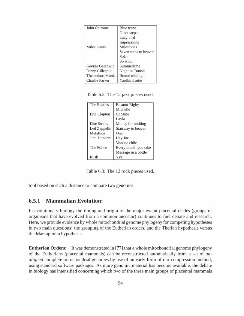
John Coltrane Blue traneGiant stepsLazy birdImpressions
Miles Davis MilestonesSeven steps to heavenSolarSo what
George Gershwin SummertimeDizzy Gillespie Night in TunisiaThelonious Monk Round midnightCharlie Parker Yardbird suite
Table 6.2: The 12 jazz pieces used.
The Beatles Eleanor RigbyMichelle
Eric Clapton CocaineLayla
Dire Straits Money for nothingLed Zeppelin Stairway to heavenMetallica OneJimi Hendrix Hey Joe
Voodoo chileThe Police Every breath you take
Message in a bottleRush Yyz
Table 6.3: The 12 rock pieces used.
tool based on such a distance to compare two genomes.
6.5.1 Mammalian Evolution:
In evolutionary biology the timing and origin of the major extant placental clades (groups oforganisms that have evolved from a common ancestor) continues to fuel debate and research.Here, we provide evidence by whole mitochondrial genome phylogeny for competing hypothesesin two main questions: the grouping of the Eutherian orders,and the Therian hypothesis versusthe Marsupionta hypothesis.
Eutherian Orders: It was demonstrated in [77] that a whole mitochondrial genome phylogenyof the Eutherians (placental mammals) can be reconstructedautomatically from a set ofun-alignedcomplete mitochondrial genomes by use of an early form of ourcompression method,using standard software packages. As more genomic materialhas become available, the debatein biology has intensified concerning which two of the three main groups of placental mammals
94
platypusopossumwallaroo
Marsupials
mouserat
Rodents
horsewhiterhino
catgraySeal
harborSealblueWhale
finWhale
Ferungulates
gibbonorangutan
gorillahuman
chimpanzeepigmyChimpanzee
Primates
Figure 6.7: The evolutionary tree built from complete mammalian mtDNA sequences of 24species, using the NCD matrix of Figure4.14on page70 where it was used to illustrate a pointof hierarchical clustering versus flat clustering. We have redrawn the tree from our output toagree better with the customary phylogeny tree format. The tree agrees exceptionally well withthe NCD distance matrix:S(T) = 0.996.
are more closely related: Primates, Ferungulates, and Rodents. In [18], the maximum likeli-hood method of phylogeny tree reconstruction gave evidencefor the (Ferungulates, (Primates,Rodents)) grouping for half of the proteins in the mitochondrial genomes investigated, and (Ro-dents, (Ferungulates, Primates)) for the other halves of the mt genomes. In that experiment theyaligned 12 concatenated mitochondrial proteins, taken from 20 species: the humble rat (Rattusnorvegicus), house mouse (Mus musculus), grey seal (Halichoerus grypus), harbor seal (Phocavitulina), cat (Felis catus), white rhino (Ceratotherium simum), horse (Equus caballus), finbackwhale (Balaenoptera physalus), blue whale (Balaenoptera musculus), cow (Bos taurus), gibbon(Hylobates lar), gorilla (Gorilla gorilla ), human (Homo sapiens), chimpanzee (Pan troglodytes),pygmy chimpanzee (Pan paniscus), orangutan (Pongo pygmaeus), Sumatran orangutan (Pongopygmaeus abelii), using opossum (Didelphis virginiana), wallaroo (Macropus robustus), and theplatypus (Ornithorhynchus anatinus) as outgroup. In [80, 77] we used the whole mitochondrialgenome of the same 20 species, computing the NCD distances (or a closely related distance in[80]), using the GenCompress compressor, followed by tree reconstruction using the neighborjoining program in the MOLPHY package [99] to confirm the commonly believed morphology-supported hypothesis (Rodents, (Primates, Ferungulates)). Repeating the experiment using thehypercleaning method [13] of phylogeny tree reconstruction gave the same result. Here, we re-peated this experiment several times using the CompLearn Toolkit using our new quartet methodfor reconstructing trees, and computing the NCD with various compressors (gzip, bzip2, PPMZ),again always with the same result. These experiments are notreported since they are subsumedby the larger experiment of Figure6.7.
95
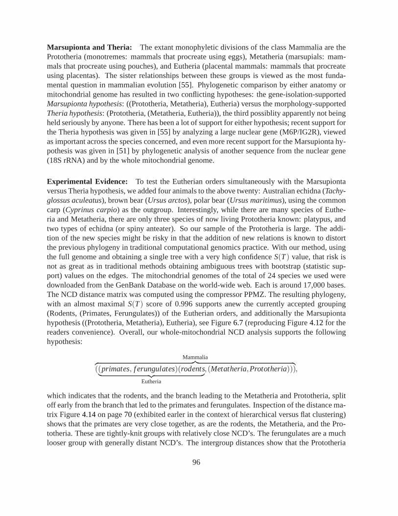
Marsupionta and Theria: The extant monophyletic divisions of the class Mammalia arethePrototheria (monotremes: mammals that procreate using eggs), Metatheria (marsupials: mam-mals that procreate using pouches), and Eutheria (placental mammals: mammals that procreateusing placentas). The sister relationships between these groups is viewed as the most funda-mental question in mammalian evolution [55]. Phylogenetic comparison by either anatomy ormitochondrial genome has resulted in two conflicting hypotheses: the gene-isolation-supportedMarsupionta hypothesis: ((Prototheria, Metatheria), Eutheria) versus the morphology-supportedTheria hypothesis: (Prototheria, (Metatheria, Eutheria)), the third possiblity apparently not beingheld seriously by anyone. There has been a lot of support for either hypothesis; recent support forthe Theria hypothesis was given in [55] by analyzing a large nuclear gene (M6P/IG2R), viewedas important across the species concerned, and even more recent support for the Marsupionta hy-pothesis was given in [51] by phylogenetic analysis of another sequence from the nuclear gene(18S rRNA) and by the whole mitochondrial genome.
Experimental Evidence: To test the Eutherian orders simultaneously with the Marsupiontaversus Theria hypothesis, we added four animals to the abovetwenty: Australian echidna (Tachy-glossus aculeatus), brown bear (Ursus arctos), polar bear (Ursus maritimus), using the commoncarp (Cyprinus carpio) as the outgroup. Interestingly, while there are many species of Euthe-ria and Metatheria, there are only three species of now living Prototheria known: platypus, andtwo types of echidna (or spiny anteater). So our sample of thePrototheria is large. The addi-tion of the new species might be risky in that the addition of new relations is known to distortthe previous phylogeny in traditional computational genomics practice. With our method, usingthe full genome and obtaining a single tree with a very high confidenceS(T) value, that risk isnot as great as in traditional methods obtaining ambiguous trees with bootstrap (statistic sup-port) values on the edges. The mitochondrial genomes of the total of 24 species we used weredownloaded from the GenBank Database on the world-wide web.Each is around 17,000 bases.The NCD distance matrix was computed using the compressor PPMZ. The resulting phylogeny,with an almost maximalS(T) score of 0.996 supports anew the currently accepted grouping(Rodents, (Primates, Ferungulates)) of the Eutherian orders, and additionally the Marsupiontahypothesis ((Prototheria, Metatheria), Eutheria), see Figure6.7(reproducing Figure4.12for thereaders convenience). Overall, our whole-mitochondrial NCD analysis supports the followinghypothesis:
Mammalia︷ ︸︸ ︷
((primates, f erungulates)(rodents︸ ︷︷ ︸
Eutheria
,(Metatheria,Prototheria))),
which indicates that the rodents, and the branch leading to the Metatheria and Prototheria, splitoff early from the branch that led to the primates and ferungulates. Inspection of the distance ma-trix Figure4.14on page70 (exhibited earler in the context of hierarchical versus flatclustering)shows that the primates are very close together, as are the rodents, the Metatheria, and the Pro-totheria. These are tightly-knit groups with relatively close NCD’s. The ferungulates are a muchlooser group with generally distant NCD’s. The intergroup distances show that the Prototheria
96
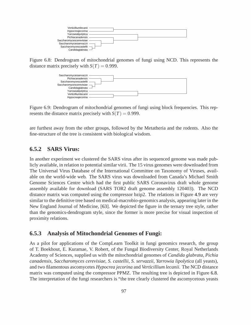
VerticilliumlecaniiHypocreajecorinaYarrowialipolyticaPichiacanadensis
SaccharomycescerevisiaeSaccharomycesservazzii
SaccharomycescastelliiCandidaglabrata
Figure 6.8: Dendrogram of mitochondrial genomes of fungi using NCD. This represents thedistance matrix precisely withS(T) = 0.999.
SaccharomycesservazziiPichiacanadensis
SaccharomycescastelliiSaccharomycescerevisiae
CandidaglabrataYarrowialipolyticaVerticilliumlecaniiHypocreajecorina
Figure 6.9: Dendrogram of mitochondrial genomes of fungi using block frequencies. This rep-resents the distance matrix precisely withS(T) = 0.999.
are furthest away from the other groups, followed by the Metatheria and the rodents. Also thefine-structure of the tree is consistent with biological wisdom.
6.5.2 SARS Virus:
In another experiment we clustered the SARS virus after its sequenced genome was made pub-licly available, in relation to potential similar virii. The 15 virus genomes were downloaded fromThe Universal Virus Database of the International Committee on Taxonomy of Viruses, avail-able on the world-wide web. The SARS virus was downloaded from Canada’s Michael SmithGenome Sciences Centre which had the first public SARS Coronavirus draft whole genomeassembly available for download (SARS TOR2 draft genome assembly 120403). The NCDdistance matrix was computed using the compressor bzip2. The relations in Figure4.9are verysimilar to the definitive tree based on medical-macrobio-genomics analysis, appearing later in theNew England Journal of Medicine, [63]. We depicted the figure in the ternary tree style, ratherthan the genomics-dendrogram style, since the former is more precise for visual inspection ofproximity relations.
6.5.3 Analysis of Mitochondrial Genomes of Fungi:
As a pilot for applications of the CompLearn Toolkit in fungigenomics research, the groupof T. Boekhout, E. Kuramae, V. Robert, of the Fungal Biodiversity Center, Royal NetherlandsAcademy of Sciences, supplied us with the mitochondrial genomes ofCandida glabrata, Pichiacanadensis, Saccharomyces cerevisiae, S. castellii, S. servazzii, Yarrowia lipolytica(all yeasts),and two filamentous ascomycetesHypocrea jecorinaandVerticillium lecanii. The NCD distancematrix was computed using the compressor PPMZ. The resulting tree is depicted in Figure6.8.The interpretation of the fungi researchers is “the tree clearly clustered the ascomycetous yeasts
97

SomaliNdebele
RundiKicongoBemba
ZapotecoChickasaw
MazahuaPurhepecha
DagaareDitammari
EnglishSpanish
DutchGerman
Figure 6.10: Clustering of Native-American, Native-African, and Native-European languages.S(T) = 0.928.
versus the two filamentous Ascomycetes, thus supporting thecurrent hypothesis on their classi-fication (for example, see [65]). Interestingly, in a recent treatment of the Saccharomycetaceae,S. servazii, S. castellii and C. glabrata were all proposed to belong to genera different fromSaccharomyces, and this is supported by the topology of our tree as well [64].”
To compare the veracity of the NCD clustering with a more feature-based clustering, we alsocalculated the pairwise distances as follows: Each file is converted to a 4096-dimensional vectorby considering the frequency of all (overlapping) 6-byte contiguous blocks. The l2-distance(Euclidean distance) is calculated between each pair of files by taking the square root of the sumof the squares of the component-wise differences. These distances are arranged into a distancematrix and linearly scaled to fit the range[0,1.0]. Finally, we ran the clustering routine on thisdistance matrix. The results are in Figure6.9. As seen by comparing with the NCD-basedFigure 6.8 there are apparent misplacements when using the Euclidean distance in this way.Thus, in this simple experiment, the NCD performed better, that is, agreed more precisely withaccepted biological knowledge.
6.6 Language Trees
Our method improves the results of [8], using a linguistic corpus of “The Universal Declarationof Human Rights (UDoHR)” [27] in 52 languages. Previously, [8] used an asymmetric measurebased on relative entropy, and the full matrix of the pair-wise distances between all 52 languages,to build a language classification tree. This experiment wasrepeated (resulting in a somewhatbetter tree) using the compression method in [77] using standard biological software packagesto construct the phylogeny. We have redone this experiment,and done new experiments, usingthe CompLearn Toolkit. Here, we report on an experiment to separate radically different lan-guage families. We downloaded the language versions of the UDoHR text in English, Spanish,Dutch, German (Native-European), Pemba, Dendi, Ndbele, Kicongo, Somali, Rundi, Ditammari,Dagaare (Native African), Chikasaw, Perhupecha, Mazahua,Zapoteco (Native-American), anddidn’t preprocess them except for removing initial identifying information. We used an Lempel-Ziv-type compressorgzip to compress text sequences of sizes not exceeding the lengthof the
98
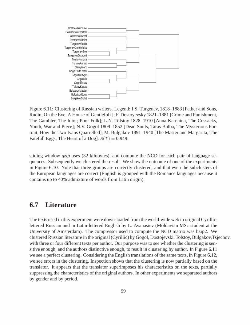
DostoevskiiCrimeDostoevskiiPoorfolk
DostoevskiiGmblDostoevskiiIdiotTurgenevRudin
TurgenevGentlefolksTurgenevEve
TurgenevOtcydetiTolstoyIunostiTolstoyAnnakTolstoyWar1
GogolPortrDvaivGogolMertvye
GogolDikGogolTaras
TolstoyKasakBulgakovMaster
BulgakovEggsBulgakovDghrt
Figure 6.11: Clustering of Russian writers. Legend: I.S. Turgenev, 1818–1883 [Father and Sons,Rudin, On the Eve, A House of Gentlefolk]; F. Dostoyevsky 1821–1881 [Crime and Punishment,The Gambler, The Idiot; Poor Folk]; L.N. Tolstoy 1828–1910 [Anna Karenina, The Cossacks,Youth, War and Piece]; N.V. Gogol 1809–1852 [Dead Souls, Taras Bulba, The Mysterious Por-trait, How the Two Ivans Quarrelled]; M. Bulgakov 1891–1940[The Master and Margarita, TheFatefull Eggs, The Heart of a Dog].S(T) = 0.949.
sliding windowgzip uses (32 kilobytes), and compute the NCD for each pair of language se-quences. Subsequently we clustered the result. We show the outcome of one of the experimentsin Figure6.10. Note that three groups are correctly clustered, and that even the subclusters ofthe European languages are correct (English is grouped withthe Romance languages because itcontains up to 40% admixture of words from Latin origin).
6.7 Literature
The texts used in this experiment were down-loaded from the world-wide web in original Cyrillic-lettered Russian and in Latin-lettered English by L. Avanasiev (Moldavian MSc student at theUniversity of Amsterdam). The compressor used to compute the NCD matrix was bzip2. Weclustered Russian literature in the original (Cyrillic) byGogol, Dostojevski, Tolstoy, Bulgakov,Tsjechov,with three or four different texts per author. Our purpose was to see whether the clustering is sen-sitive enough, and the authors distinctive enough, to result in clustering by author. In Figure6.11we see a perfect clustering. Considering the English translations of the same texts, in Figure6.12,we see errors in the clustering. Inspection shows that the clustering is now partially based on thetranslator. It appears that the translator superimposes his characteristics on the texts, partiallysuppressing the characteristics of the original authors. In other experiments we separated authorsby gender and by period.
99
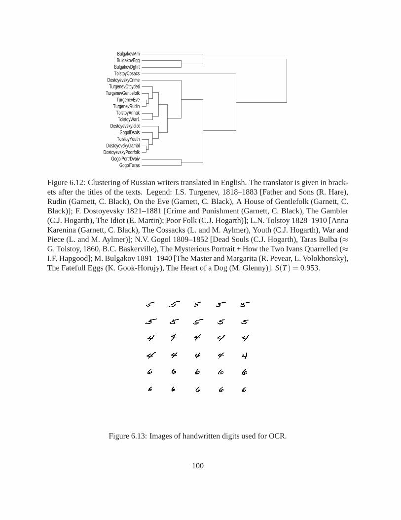
BulgakovMmBulgakovEgg
BulgakovDghrtTolstoyCosacs
DostoyevskyCrimeTurgenevOtcydeti
TurgenevGentlefolkTurgenevEve
TurgenevRudinTolstoyAnnakTolstoyWar1
DostoyevskyIdiotGogolDsols
TolstoyYouthDostoyevskyGambl
DostoyevskyPoorfolkGogolPortrDvaiv
GogolTaras
Figure 6.12: Clustering of Russian writers translated in English. The translator is given in brack-ets after the titles of the texts. Legend: I.S. Turgenev, 1818–1883 [Father and Sons (R. Hare),Rudin (Garnett, C. Black), On the Eve (Garnett, C. Black), A House of Gentlefolk (Garnett, C.Black)]; F. Dostoyevsky 1821–1881 [Crime and Punishment (Garnett, C. Black), The Gambler(C.J. Hogarth), The Idiot (E. Martin); Poor Folk (C.J. Hogarth)]; L.N. Tolstoy 1828–1910 [AnnaKarenina (Garnett, C. Black), The Cossacks (L. and M. Aylmer), Youth (C.J. Hogarth), War andPiece (L. and M. Aylmer)]; N.V. Gogol 1809–1852 [Dead Souls (C.J. Hogarth), Taras Bulba (≈G. Tolstoy, 1860, B.C. Baskerville), The Mysterious Portrait + How the Two Ivans Quarrelled (≈I.F. Hapgood]; M. Bulgakov 1891–1940 [The Master and Margarita (R. Pevear, L. Volokhonsky),The Fatefull Eggs (K. Gook-Horujy), The Heart of a Dog (M. Glenny)]. S(T) = 0.953.
Figure 6.13: Images of handwritten digits used for OCR.
100
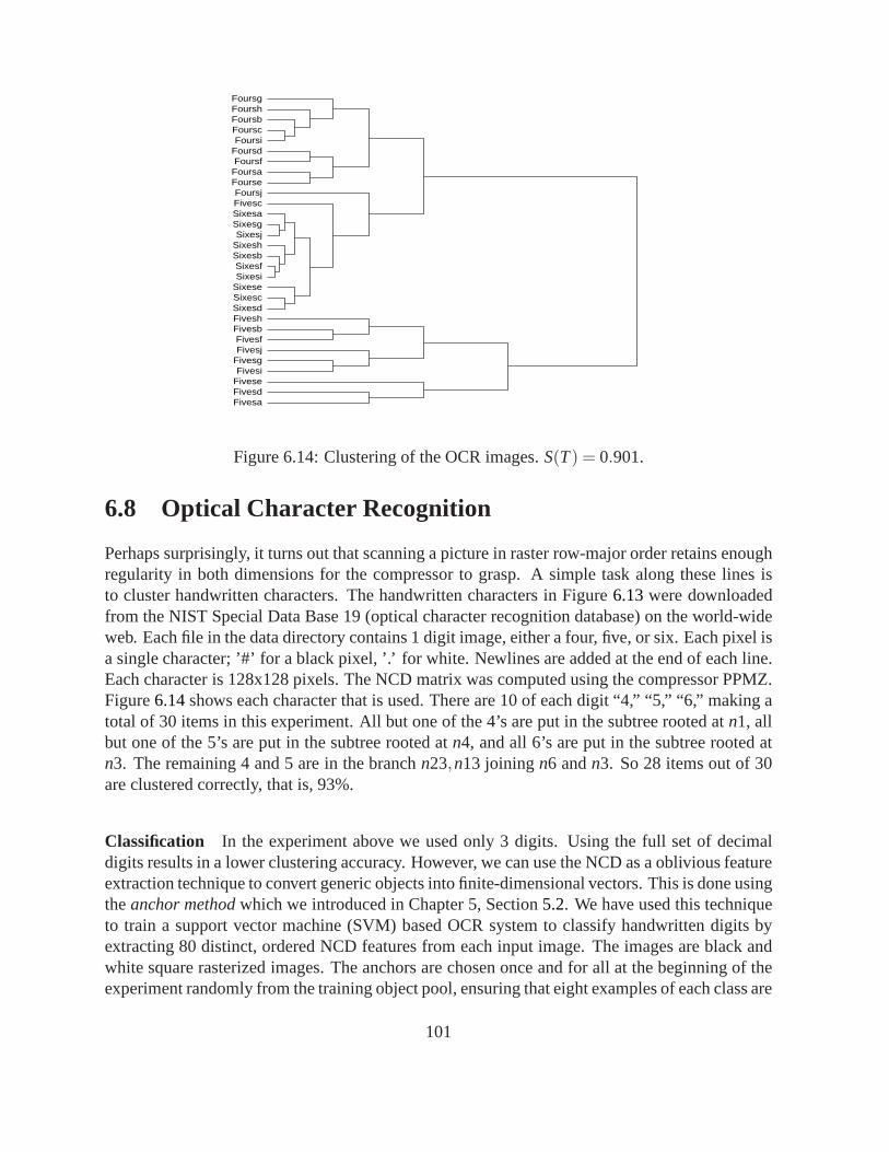
FoursgFourshFoursbFourscFoursi
FoursdFoursf
FoursaFourseFoursjFivescSixesaSixesgSixesj
SixeshSixesbSixesfSixesi
SixeseSixescSixesdFiveshFivesbFivesfFivesj
FivesgFivesi
FiveseFivesdFivesa
Figure 6.14: Clustering of the OCR images.S(T) = 0.901.
6.8 Optical Character Recognition
Perhaps surprisingly, it turns out that scanning a picture in raster row-major order retains enoughregularity in both dimensions for the compressor to grasp. Asimple task along these lines isto cluster handwritten characters. The handwritten characters in Figure6.13were downloadedfrom the NIST Special Data Base 19 (optical character recognition database) on the world-wideweb. Each file in the data directory contains 1 digit image, either a four, five, or six. Each pixel isa single character; ’#’ for a black pixel, ’.’ for white. Newlines are added at the end of each line.Each character is 128x128 pixels. The NCD matrix was computed using the compressor PPMZ.Figure6.14shows each character that is used. There are 10 of each digit “4,” “5,” “6,” making atotal of 30 items in this experiment. All but one of the 4’s areput in the subtree rooted atn1, allbut one of the 5’s are put in the subtree rooted atn4, and all 6’s are put in the subtree rooted atn3. The remaining 4 and 5 are in the branchn23,n13 joiningn6 andn3. So 28 items out of 30are clustered correctly, that is, 93%.
Classification In the experiment above we used only 3 digits. Using the full set of decimaldigits results in a lower clustering accuracy. However, we can use the NCD as a oblivious featureextraction technique to convert generic objects into finite-dimensional vectors. This is done usingtheanchor methodwhich we introduced in Chapter 5, Section5.2. We have used this techniqueto train a support vector machine (SVM) based OCR system to classify handwritten digits byextracting 80 distinct, ordered NCD features from each input image. The images are black andwhite square rasterized images. The anchors are chosen onceand for all at the beginning of theexperiment randomly from the training object pool, ensuring that eight examples of each class are
101

chosen. Once chosen, the anchors are kept in order (so that the first coordinate always refers tothe same anchor and so on) and used to translate all other training data files into 80-dimensionalvectors. In this initial stage of ongoing research, by our oblivious method of compression-basedclustering to supply a kernel for an SVM classifier, we achieved a handwritten single decimaldigit recognition accuracy of 85%. The current state-of-the-art for this problem, after half acentury of interactive feature-driven classification research, in the upper ninety % level [87, 113].All experiments are bench marked on the standard NIST Special Data Base 19 (optical characterrecognition database).
6.9 Astronomy
As a proof of principle we clustered data from unknown objects, for example objects that are faraway. In [5] observations of the microquasar GRS 1915+105 made with theRossi X-ray Tim-ing Explorer were analyzed. The interest in this microquasar stems from the fact that it was thefirst Galactic object to show a certain behavior (superluminal expansion in radio observations).Photonometric observation data from X-ray telescopes weredivided into short time segments(usually in the order of one minute), and these segments havebeen classified into a bewilder-ing array of fifteen different modes after considerable effort. Briefly, spectrum hardness ratios(roughly, “color”) and photon count sequences were used to classify a given interval into cate-gories of variability modes. From this analysis, the extremely complex variability of this sourcewas reduced to transitions between three basic states, which, interpreted in astronomical terms,gives rise to an explanation of this peculiar source in standard black-hole theory. The data weused in this experiment made available to us by M. Klein Wolt (co-author of the above paper)and T. Maccarone, both researchers at the Astronomical Institute “Anton Pannekoek”, Universityof Amsterdam. The observations are essentially time series, and our aim was experimenting withour method as a pilot to more extensive joint research. Here the task was to see whether theclustering would agree with the classification above. The NCD matrix was computed using thecompressor PPMZ. The results are in Figure6.15. We clustered 12 objects, consisting of threeintervals from four different categories denoted asδ,γ,φ,θ in Table 1 of [5]. In Figure6.15wedenote the categories by the corresponding Roman letters D,G, P, and T, respectively. The result-ing tree groups these different modes together in a way that is consistent with the classificationby experts for these observations. The oblivious compression clustering corresponds preciselywith the laborious feature-driven classification in [5].
6.10 Conclusion
To interpret what the NCD is doing, and to explain its remarkable accuracy and robustness acrossapplication fields and compressors, the intuition is that the NCD minorizes all similarity metricsbased on features that are captured by the reference compressor involved. Such features must berelativelysimplein the sense that they are expressed by an aspect that the compressor analyzes(for example frequencies, matches, repeats). Certain sophisticated features may well be express-
102
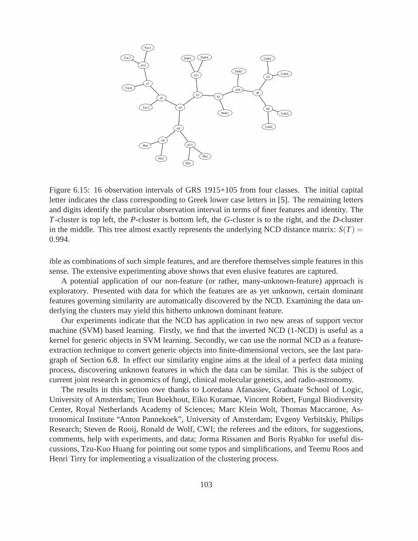
Dab1
n11
Dab4
n2
Dab2
n10
n1n0
Dab3
Gab1
n6
Gab3
Gab2
n3Gab4
Pb1
n13
n9
Pb2Pb3
n8
Pb4
Tac1
n12
n7
Tac2
Tac3
n5
n4
Tac4
Figure 6.15: 16 observation intervals of GRS 1915+105 from four classes. The initial capitalletter indicates the class corresponding to Greek lower case letters in [5]. The remaining lettersand digits identify the particular observation interval interms of finer features and identity. TheT-cluster is top left, theP-cluster is bottom left, theG-cluster is to the right, and theD-clusterin the middle. This tree almost exactly represents the underlying NCD distance matrix:S(T) =0.994.
ible as combinations of such simple features, and are therefore themselves simple features in thissense. The extensive experimenting above shows that even elusive features are captured.
A potential application of our non-feature (or rather, many-unknown-feature) approach isexploratory. Presented with data for which the features areas yet unknown, certain dominantfeatures governing similarity are automatically discovered by the NCD. Examining the data un-derlying the clusters may yield this hitherto unknown dominant feature.
Our experiments indicate that the NCD has application in twonew areas of support vectormachine (SVM) based learning. Firstly, we find that the inverted NCD (1-NCD) is useful as akernel for generic objects in SVM learning. Secondly, we canuse the normal NCD as a feature-extraction technique to convert generic objects into finite-dimensional vectors, see the last para-graph of Section6.8. In effect our similarity engine aims at the ideal of a perfect data miningprocess, discovering unknown features in which the data canbe similar. This is the subject ofcurrent joint research in genomics of fungi, clinical molecular genetics, and radio-astronomy.
The results in this section owe thanks to Loredana Afanasiev, Graduate School of Logic,University of Amsterdam; Teun Boekhout, Eiko Kuramae, Vincent Robert, Fungal BiodiversityCenter, Royal Netherlands Academy of Sciences; Marc Klein Wolt, Thomas Maccarone, As-tronomical Institute “Anton Pannekoek”, University of Amsterdam; Evgeny Verbitskiy, PhilipsResearch; Steven de Rooij, Ronald de Wolf, CWI; the refereesand the editors, for suggestions,comments, help with experiments, and data; Jorma Rissanen and Boris Ryabko for useful dis-cussions, Tzu-Kuo Huang for pointing out some typos and simplifications, and Teemu Roos andHenri Tirry for implementing a visualization of the clustering process.
103


Chapter 7
Automatic Meaning Discovery Using Google
The NCD investigations of the previous chapters focused on using data compressors to compressdata in files. This chapter deals with an entirely different sort of analysis that is not performedon files but rather onsearch termsfor the Google web search engine. By using well-known con-nections between code-lengths and probabilities, we applythe NCD theory to Google’s searchengine index, providing insight into the subjective relationships enjoyed among a group of wordsor phrases. The Google Simple Object Access Protocol is usedto connect it with the CompLearnsystem. Remarkably, the system does not use the contents of web pages directly, but instead onlyuses the estimated results count indicator from the Google search engine to make a probabilis-tic model of the web. This model is based on sampling each search term in a group as wellas all pairs in order to find structure in their co-occurrence. Before explaining the method indetail the reader is invited to have a look at the experiment in Figure7.1 involving the namesof politicians. The tree shows the subjective relationships among several European Commis-sion members. After giving a general introduction to the method, we introduce some relevantbackground material in Section7.1.2. We explain the formula that connects NCD to Google inSection7.3. We provide a sketch of one possible theoretical breakdown concerning the surpris-ing robustness of the results and consequent Google-based distance metric. We prove a certainsort of universality property for this metric. In Section7.4, we present a variety of experimentsdemonstrating the sorts of results that may be obtained. We demonstrate positive correlations,evidencing an underlying semantic structure, in both numerical symbol notations and number-name words in a variety of natural languages and contexts. Next, we demonstrate the ability todistinguish between colors and numbers, and to distinguishbetween 17th century Dutch painters;the ability to understand electrical terms, religious terms, and emergency incidents; we conduct amassive experiment in understanding WordNet categories; and finally we demonstrate the abilityto do a simple automatic English-Spanish vocabulary acquisition.
7.1 Introduction
Objects can be given literally, like the literal four-letter genome of a mouse, or the literal text ofWar and Peaceby Tolstoy. For simplicity we take it that all meaning of the object is represented
105
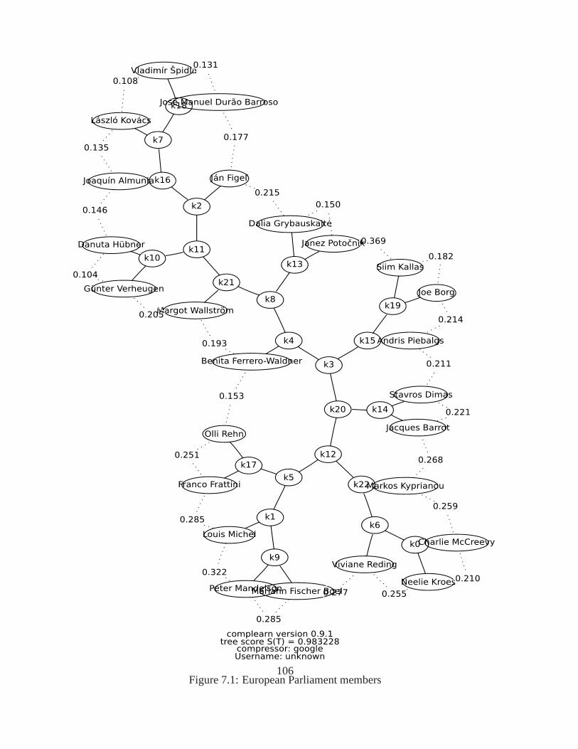
Figure 7.1: European Parliament members106
by the literal object itself. Objects can also be given by name, like “the four-letter genome of amouse,” or “the text ofWar and Peaceby Tolstoy.” There are also objects that cannot be givenliterally, but only by name, and that acquire their meaning from their contexts in backgroundcommon knowledge in humankind, like “home” or “red.” To makecomputers more intelligentone would like to represent meaning in computer digestible form. Long-term and labor-intensiveefforts like theCycproject [71] and theWordNetproject [37] try to establish semantic relationsbetween common objects, or, more precisely,namesfor those objects. The idea is to create asemantic web of such vast proportions that rudimentary intelligence, and knowledge about thereal world, spontaneously emerge. This comes at the great cost of designing structures capableof manipulating knowledge, and entering high quality contents in these structures by knowledge-able human experts. While the efforts are long-running and large scale, the overall informationentered is minute compared to what is available on the world-wide-web.
The rise of the world-wide-web has enticed millions of usersto type in trillions of charactersto create billions of web pages of on average low quality contents. The sheer mass of the informa-tion available about almost every conceivable topic makes it likely that extremes will cancel andthe majority or average is meaningful in a low-quality approximate sense. We devise a generalmethod to tap the amorphous low-grade knowledge available for free on the world-wide-web,typed in by local users aiming at personal gratification of diverse objectives, and yet globallyachieving what is effectively the largest semantic electronic database in the world. Moreover,this database is available for all by using any search enginethat can return aggregate page-countestimates for a large range of search queries, like Google.
Previously, we and others developed a compression-based method to establish a universalsimilarity metric among objects given as finite binary strings [9, 75, 76, 26, 25, 22], which waswidely reported [85, 88, 35]; some of these experiments are shown in chapters 5 and 7. Suchobjects can be genomes, music pieces in MIDI format, computer programs in Ruby or C, picturesin simple bitmap formats, or time sequences such as heart rhythm data. This method is feature-free in the sense that it does not analyze the files looking forparticular features; rather it analyzesall features simultaneously and determines the similaritybetween every pair of objects accordingto the most dominant shared feature. The crucial point is that the method analyzes the objectsthemselves. This precludes comparison of abstract notionsor other objects that do not lendthemselves to direct analysis, like emotions, colors, Socrates, Plato, Mike Bonanno and AlbertEinstein. While the previous method that compares the objects themselves is particularly suitedto obtain knowledge about the similarity of objects themselves, irrespective of common beliefsabout such similarities, here we develop a method that uses only the name of an object andobtains knowledge about the similarity of objects by tapping available information generated bymultitudes of web users. Here we are reminded of the words of D.H. Rumsfeld [96]
“A trained ape can know an awful lotOf what is going on in this world,Just by punching on his mouseFor a relatively modest cost!”
This is useful to extract knowledge from a given corpus of knowledge, in this case the Googledatabase, but not to obtain true facts that are not common knowledge in that database. For
107

example, common viewpoints on the creation myths in different religions may be extracted bythe Googling method, but contentious questions of fact concerning the phylogeny of species canbe better approached by using the genomes of these species, rather than by opinion.
7.1.1 Googling for Knowledge
Intuitively, the approach is as follows. The Google search engine indexes around ten billionpages on the web today. Each such page can be viewed as a set of index terms. While the theorywe propose is rather intricate, the resulting method is simple enough. We give an example: Atthe time of doing the experiment, a Google search for “horse”, returned 46,700,000 hits. Thenumber of hits for the search term “rider” was 12,200,000. Searching for the pages where both“horse” and “rider” occur gave 2,630,000 hits, and Google indexed 8,058,044,651 web pages.Using these numbers in the main formula (7.3.3) we derive below, withN = 8,058,044,651, thisyields a Normalized Google Distance between the terms “horse” and “rider” as follows:
NGD(horse, rider)≈ 0.443.
In the next part of this thesis we argue that the NGD is a normedsemantic distance between theterms in question, usually (but not always, see below) inbetween 0 (identical) and 1 (unrelated),in the cognitive space invoked by the usage of the terms on theworld-wide-web as filtered byGoogle. Because of the vastness and diversity of the web thismay be taken as related to thecurrent use of the terms in society. We did the same calculation when Google indexed only one-half of the number of pages: 4,285,199,774. It is instructive that the probabilities of the usedsearch terms didn’t change significantly over this doublingof pages, with number of hits for“horse” equal 23,700,000, for “rider” equal 6,270,000, andfor “horse, rider” equal to 1,180,000.The NGD(horse, rider) we computed in that situation was≈ 0.460. This is in line with ourcontention that the relative frequencies of web pages containing search terms gives objectiveinformation about the semantic relations between the search terms. If this is the case, then theGoogle probabilities of search terms and the computed NGD ’sshould stabilize (become scaleinvariant) with a growing Google database.
7.1.2 Related Work and Background NGD
It has been brought to our attention, that there is a great deal of work in both cognitive psychology[68], linguistics, and computer science, about using word (phrases) frequencies in text corporato develop measures for word similarity or word association, partially surveyed in [112, 111],going back to at least [72]. These approaches are based on arguments and theories thatare fun-damentally different from the approach we develop, which isbased on coding and compression,based on the theory of Kolmogorov complexity [79]. This allows to express and prove propertiesof absolute relations between objects that cannot even be expressed by other approaches. TheNGD is the result of a new type of theory and as far as we know is not equivalent to any earliermeasure. Nevertheless, in practice the resulting measure may still sometimes lead to similar re-sults as existing methods. The current thesis is a next step in a decade of cumulative research in
108
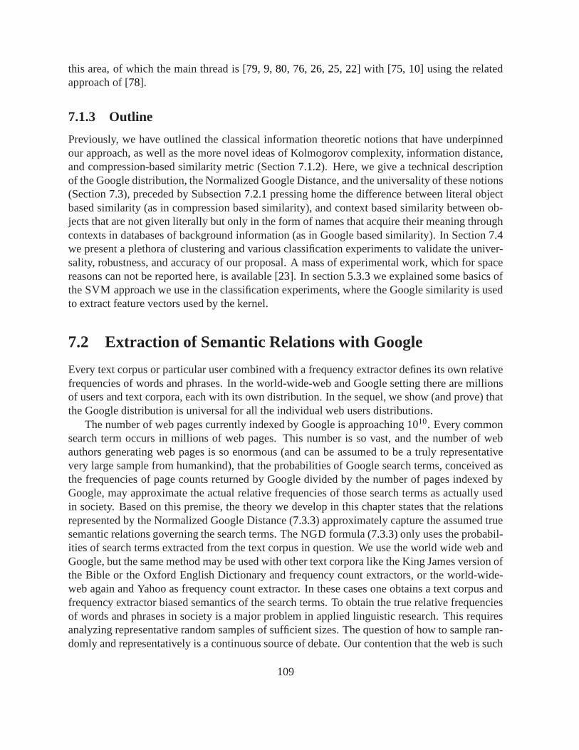
this area, of which the main thread is [79, 9, 80, 76, 26, 25, 22] with [75, 10] using the relatedapproach of [78].
7.1.3 Outline
Previously, we have outlined the classical information theoretic notions that have underpinnedour approach, as well as the more novel ideas of Kolmogorov complexity, information distance,and compression-based similarity metric (Section7.1.2). Here, we give a technical descriptionof the Google distribution, the Normalized Google Distance, and the universality of these notions(Section7.3), preceded by Subsection7.2.1pressing home the difference between literal objectbased similarity (as in compression based similarity), andcontext based similarity between ob-jects that are not given literally but only in the form of names that acquire their meaning throughcontexts in databases of background information (as in Google based similarity). In Section7.4we present a plethora of clustering and various classification experiments to validate the univer-sality, robustness, and accuracy of our proposal. A mass of experimental work, which for spacereasons can not be reported here, is available [23]. In section5.3.3we explained some basics ofthe SVM approach we use in the classification experiments, where the Google similarity is usedto extract feature vectors used by the kernel.
7.2 Extraction of Semantic Relations with Google
Every text corpus or particular user combined with a frequency extractor defines its own relativefrequencies of words and phrases. In the world-wide-web andGoogle setting there are millionsof users and text corpora, each with its own distribution. Inthe sequel, we show (and prove) thatthe Google distribution is universal for all the individualweb users distributions.
The number of web pages currently indexed by Google is approaching 1010. Every commonsearch term occurs in millions of web pages. This number is sovast, and the number of webauthors generating web pages is so enormous (and can be assumed to be a truly representativevery large sample from humankind), that the probabilities of Google search terms, conceived asthe frequencies of page counts returned by Google divided bythe number of pages indexed byGoogle, may approximate the actual relative frequencies ofthose search terms as actually usedin society. Based on this premise, the theory we develop in this chapter states that the relationsrepresented by the Normalized Google Distance (7.3.3) approximately capture the assumed truesemantic relations governing the search terms. The NGD formula (7.3.3) only uses the probabil-ities of search terms extracted from the text corpus in question. We use the world wide web andGoogle, but the same method may be used with other text corpora like the King James version ofthe Bible or the Oxford English Dictionary and frequency count extractors, or the world-wide-web again and Yahoo as frequency count extractor. In these cases one obtains a text corpus andfrequency extractor biased semantics of the search terms. To obtain the true relative frequenciesof words and phrases in society is a major problem in applied linguistic research. This requiresanalyzing representative random samples of sufficient sizes. The question of how to sample ran-domly and representatively is a continuous source of debate. Our contention that the web is such
109

a large and diverse text corpus, and Google such an able extractor, that the relative page countsapproximate the true societal word- and phrases usage, starts to be supported by current reallinguistics research [100].
Similarly, the NGD minorizes and incorporates all the different semantics of all the differentusers and text corpora on the web. It extracts as it were the semantics as used in the society (of allthese web users) and not just the bias of any individual user or document. This is only possibleusing the web, since its sheer mass of users and documents with different intentions averagesout to give the true semantic meaning as used in society. Thisis experimentally evidenced bythe fact that when Google doubled its size the sample semantics of rider, horse stayed the same.Determining the NGD between two Google search terms does notinvolve analysis of particularfeatures or specific background knowledge of the problem area. Instead, it analyzes all featuresautomatically through Google searches of the most general background knowledge data base: theworld-wide-web. (In Statistics “parameter-free estimation” means that the number of parametersanalyzed is infinite or not a priori restricted. In our setting “feature-freeness” means that weanalyze all features.)
7.2.1 Genesis of the Approach
We start from the observation that a compressor defines a codeword length for every sourceword, namely, the number of bits in the compressed version ofthat source word. Viewing thiscode as a Shannon-Fano code, Section2.7, it defines in its turn a probability mass function onthe source words. Conversely, every probability mass function of the source words defines aShannon-Fano code of the source words. Since this code is optimally compact in the sense ofhaving expected code-word length equal to the entropy of theinitial probability mass function,we take the viewpoint that a probability mass function is a compressor.
7.2.1.EXAMPLE . For example, the NID (Normalized Information Distance, Chapter 3, Sec-tion 3.3) uses the probability mass functionm(x) = 2−K(x), whereK is the Kolmogorov com-plexity function, Chapter 2. This function is not computable, but it has the weaker propertyof being lower semi-computable: by approximatingK(x) from above by better and better com-pressors, we approximatem(x) from below. The distributionm(x) has the remarkable propertythat it dominates every lower semi-computable probabilitymass functionP(x) (and hence allcomputable ones) by assigning more probability to every finite binary stringx thanP(x), up toa multiplicative constantcP > 0 depending onP but not onx (m(x) ≥ cPP(x)). We say thatm(x) is universalfor the enumeration of all lower semi-computable probability mass functions,[79], a terminology that is closely related to the “universality” of a universal Turing machinein the enumeration of all Turing machines. It is this property that allows us to show [76] thatNID is themost informativedistance (actually a metric) among a large family of (possibly non-metric) “admissible normalized information distances.” But we cannot apply these same formalclaims to the real-world NCD , except in a sense that is relativized on how well the compressorapproximates the ultimate Kolmogorov complexity [22, 26, 25] and as shown in Section3.3.
In essence, the choice of compressor brings a particular setof assumptions to bear upon anincoming data stream, and if these assumptions turn out to beaccurate for the data in question,
110
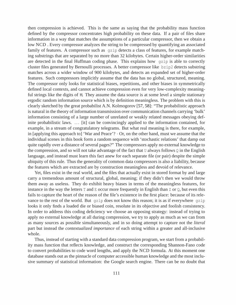
then compression is achieved. This is the same as saying thatthe probability mass functiondefined by the compressor concentrates high probability on these data. If a pair of files shareinformation in a way that matches the assumptions of a particular compressor, then we obtain alow NCD . Every compressor analyzes the string to be compressed by quantifying an associatedfamily of features. A compressor such asgzip detects a class of features, for example match-ing substrings that are separated by no more than 32 kilobytes. Certain higher-order similaritiesare detected in the final Huffman coding phase. This explainshow gzip is able to correctlycluster files generated by Bernoulli processes. A better compressor likebzip2 detects substringmatches across a wider window of 900 kilobytes, and detects an expanded set of higher-orderfeatures. Such compressors implicitly assume that the datahas no global, structured, meaning.The compressor only looks for statistical biases, repetitions, and other biases in symmetricallydefined local contexts, and cannot achieve compression evenfor very low-complexity meaning-ful strings like the digits ofπ. They assume the data source is at some level a simple stationaryergodic random information source which is by definition meaningless. The problem with this isclearly sketched by the great probabilist A.N. Kolmogorov [57, 58]: “The probabilistic approachis natural in the theory of information transmission over communication channels carrying ‘bulk’information consisting of a large number of unrelated or weakly related messages obeying def-inite probabilistic laws.. . . [it] can be convincingly applied to the information contained, forexample, in a stream of congratulatory telegrams. But what real meaning is there, for example,in [applying this approach to] ‘War and Peace’?· Or, on the other hand, must we assume that theindividual scenes in this book form a random sequence with ‘stochastic relations’ that damp outquite rapidly over a distance of several pages?” The compressors apply no external knowledge tothe compression, and so will not take advantage of the fact thatU always followsQ in the Englishlanguage, and instead must learn this fact anew for each separate file (or pair) despite the simpleubiquity of this rule. Thus the generality of common data compressors is also a liability, becausethe features which are extracted are by construction meaningless and devoid of relevance.
Yet, files exist in the real world, and the files that actually exist in stored format by and largecarry a tremendous amount of structural, global, meaning; if they didn’t then we would throwthem away as useless. They do exhibit heavy biases in terms ofthe meaningless features, forinstance in the way the lettersT andE occur more frequently in English thanZ or Q, but even thisfails to capture the heart of the reason of the file’s existence in the first place: because of its rele-vance to the rest of the world. Butgzip does not know this reason; it is as if everywheregziplooks it only finds a loaded die or biased coin, resolute in itsobjective and foolish consistency.In order to address this coding deficiency we choose an opposing strategy: instead of trying toapply no external knowledge at all during compression, we try to apply as much as we can fromas many sources as possible simultaneously, and in so doing attempt to capture not theliteralpart but instead thecontextualized importanceof each string within a greater and all-inclusivewhole.
Thus, instead of starting with a standard data compression program, we start from a probabil-ity mass function that reflects knowledge, and construct thecorresponding Shannon-Fano codeto convert probabilities to code word lengths, and apply theNCD formula. At this moment onedatabase stands out as the pinnacle of computer accessible human knowledge and the most inclu-sive summary of statistical information: the Google searchengine. There can be no doubt that
111
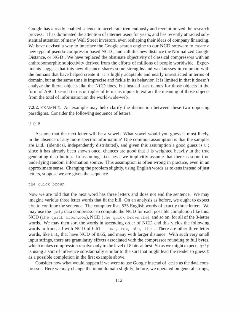
Google has already enabled science to accelerate tremendously and revolutionized the researchprocess. It has dominated the attention of internet users for years, and has recently attracted sub-stantial attention of many Wall Street investors, even reshaping their ideas of company financing.We have devised a way to interface the Google search engine toour NCD software to create anew type of pseudo-compressor based NCD , and call this new distance the Normalized GoogleDistance, or NGD . We have replaced the obstinate objectivity of classical compressors with ananthropomorphic subjectivity derived from the efforts of millions of people worldwide. Exper-iments suggest that this new distance shares some strengthsand weaknesses in common withthe humans that have helped create it: it is highly adaptableand nearly unrestricted in terms ofdomain, but at the same time is imprecise and fickle in its behavior. It is limited in that it doesn’tanalyze the literal objects like the NCD does, but instead uses names for those objects in theform of ASCII search terms or tuples of terms as inputs to extract the meaning of those objectsfrom the total of information on the world-wide-web.
7.2.2.EXAMPLE . An example may help clarify the distinction between these two opposingparadigms. Consider the following sequence of letters:
U Q B
Assume that the next letter will be a vowel. What vowel would you guess is most likely,in the absence of any more specific information? One common assumption is that the samplesare i.i.d. (identical, independently distributed), and given this assumption a good guess isU ;since it has already been shown once, chances are good thatU is weighted heavily in the truegenerating distribution. In assuming i.i.d.-ness, we implicitly assume that there is some trueunderlying random information source. This assumption is often wrong in practice, even in anapproximate sense. Changing the problem slightly, using English words as tokens instead of justletters, suppose we are given the sequence
the quick brown
Now we are told that the next word has three letters and does not end the sentence. We mayimagine various three letter words that fit the bill. On an analysis as before, we ought to expectthe to continue the sentence. The computer lists 535 English words of exactly three letters. Wemay use thegzip data compressor to compute the NCD for each possible completion like this:NCD (the quick brown,cow), NCD (the quick brown,the), and so on, for all of the 3-letterwords. We may then sort the words in ascending order of NCD andthis yields the followingwords in front, all with NCD of 0.61: own, row, she, the . There are other three letterwords, likehot, that have NCD of 0.65, and many with larger distance. With such very smallinput strings, there are granularity effects associated with the compressor rounding to full bytes,which makes compression resolve only to the level of 8 bits atbest. So as we might expect,gzipis using a sort of inference substantially similar to the sort that might lead the reader to guessUas a possible completion in the first example above.
Consider now what would happen if we were to use Google instead of gzip as the data com-pressor. Here we may change the input domain slightly; before, we operated on general strings,
112
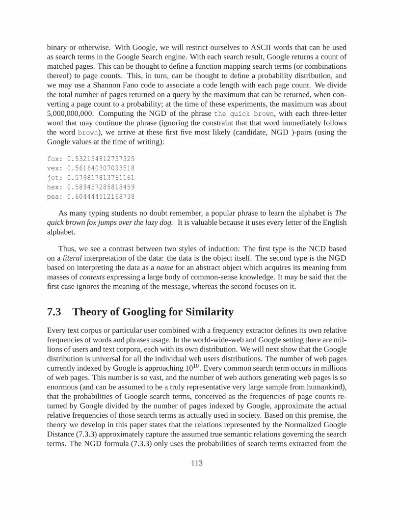
binary or otherwise. With Google, we will restrict ourselves to ASCII words that can be usedas search terms in the Google Search engine. With each searchresult, Google returns a count ofmatched pages. This can be thought to define a function mapping search terms (or combinationsthereof) to page counts. This, in turn, can be thought to define a probability distribution, andwe may use a Shannon Fano code to associate a code length with each page count. We dividethe total number of pages returned on a query by the maximum that can be returned, when con-verting a page count to a probability; at the time of these experiments, the maximum was about5,000,000,000. Computing the NGD of the phrasethe quick brown, with each three-letterword that may continue the phrase (ignoring the constraint that that word immediately followsthe wordbrown), we arrive at these first five most likely (candidate, NGD )-pairs (using theGoogle values at the time of writing):
fox: 0.532154812757325vex: 0.561640307093518jot: 0.579817813761161hex: 0.589457285818459pea: 0.604444512168738
As many typing students no doubt remember, a popular phrase to learn the alphabet isThequick brown fox jumps over the lazy dog.It is valuable because it uses every letter of the Englishalphabet.
Thus, we see a contrast between two styles of induction: The first type is the NCD basedon aliteral interpretation of the data: the data is the object itself. The second type is the NGDbased on interpreting the data as anamefor an abstract object which acquires its meaning frommasses ofcontextsexpressing a large body of common-sense knowledge. It may besaid that thefirst case ignores the meaning of the message, whereas the second focuses on it.
7.3 Theory of Googling for Similarity
Every text corpus or particular user combined with a frequency extractor defines its own relativefrequencies of words and phrases usage. In the world-wide-web and Google setting there are mil-lions of users and text corpora, each with its own distribution. We will next show that the Googledistribution is universal for all the individual web users distributions. The number of web pagescurrently indexed by Google is approaching 1010. Every common search term occurs in millionsof web pages. This number is so vast, and the number of web authors generating web pages is soenormous (and can be assumed to be a truly representative very large sample from humankind),that the probabilities of Google search terms, conceived asthe frequencies of page counts re-turned by Google divided by the number of pages indexed by Google, approximate the actualrelative frequencies of those search terms as actually usedin society. Based on this premise, thetheory we develop in this paper states that the relations represented by the Normalized GoogleDistance (7.3.3) approximately capture the assumed true semantic relations governing the searchterms. The NGD formula (7.3.3) only uses the probabilities of search terms extracted fromthe
113
text corpus in question. We use the world-wide-web and Google, but the same method may beused with other text corpora like the King James version of the Bible or the Oxford English Dic-tionary and frequency count extractors, or the world-wide-web again and Yahoo as frequencycount extractor. In these cases one obtains a text corpus andfrequency extractor biased seman-tics of the search terms. To obtain the true relative frequencies of words and phrases in societyis a major problem in applied linguistic research. This requires analyzing representative randomsamples of sufficient sizes. The question of how to sample randomly and representatively is acontinuous source of debate. Our contention that the web is such a large and diverse text corpus,and Google such an able extractor, that the relative page counts approximate the true societalword- and phrases usage, starts to be supported by current real linguistics research [100].
7.3.1 The Google Distribution:
Let the set of singletonGoogle search termsbe denoted byS . In the sequel we use both singletonsearch terms and doubleton search termsx,y : x,y ∈ S . Let the set of web pages indexed(possible of being returned) by Google beΩ. The cardinality ofΩ is denoted byM = |Ω|, and atthe time of this writing 8·109≤M ≤ 9·109 (and presumably greater by the time of reading this).Assume that a priori all web pages are equi-probable, with the probability of being returned byGoogle being 1/M. A subset ofΩ is called anevent. Everysearch term xusable by Googledefines asingleton Google eventx ⊆ Ω of web pages that contain an occurrence ofx and arereturned by Google if we do a search forx. Let L : Ω→ [0,1] be the uniform mass probabilityfunction. The probability of an eventx is L(x) = |x|/M. Similarly, thedoubleton Google eventx
T
y⊆Ω is the set of web pages returned by Google if we do a search for pages containing bothsearch termx and search termy. The probability of this event isL(x
T
y) = |xT
y|/M. We canalso define the other Boolean combinations:¬x = Ω\x andx
S
y =¬(¬xT¬y), each such event
having a probability equal to its cardinality divided byM. If e is an event obtained from the basiceventsx,y, . . ., corresponding to basic search termsx,y, . . ., by finitely many applications of theBoolean operations, then the probabilityL(e) = |e|/M.
7.3.2 Google Semantics:
Google events capture in a particular sense all background knowledge about the search termsconcerned available (to Google) on the web.
The Google eventx, consisting of the set of all web pages containing one or moreoccurrences of the search termx, thus embodies, in every possible sense, all directcontext in whichx occurs on the web. This constitutes the Google semantics of theterm.
7.3.1.REMARK . It is of course possible that parts of this direct contextual material link to otherweb pages in whichx does not occur and thereby supply additional context. In ourapproach thisindirect context is ignored. Nonetheless, indirect context may be important and future refine-ments of the method may take it into account.
114
7.3.3 The Google Code:
The eventx consists of all possible direct knowledge on the web regarding x. Therefore, it isnatural to consider code words for those events as coding this background knowledge. However,we cannot use the probability of the events directly to determine a prefix code, or, rather theunderlying information content implied by the probability. The reason is that the events over-lap and hence the summed probability exceeds 1. By the Kraft inequality [31] this prevents acorresponding set of code-word lengths. The solution is to normalize: We use the probabilityof the Google events to define a probability mass function over the setx,y : x,y ∈ S ofGoogle search terms, both singleton and doubleton terms. There are|S | singleton terms, and(|S |
2
)doubletons consisting of a pair of non-identical terms. Define
N = ∑x,y⊆S
|x\
y|,
counting each singleton set and each doubleton set (by definition unordered) once in the sum-mation. Note that this means that for every pairx,y ⊆ S , with x 6= y, the web pagesz∈ x
T
yare counted three times: once inx = x
T
x, once iny = yT
y, and once inxT
y. Since everyweb page that is indexed by Google contains at least one occurrence of a search term, we haveN ≥ M. On the other hand, web pages contain on average not more thana certain constantαsearch terms. Therefore,N≤ αM. Define
g(x) = g(x,x), g(x,y) = L(x\
y)M/N = |x\
y|/N. (7.3.1)
Then,∑x,y⊆S g(x,y) = 1. Thisg-distribution changes over time, and between different sam-plings from the distribution. But let us imagine thatg holds in the sense of an instantaneoussnapshot. The real situation will be an approximation of this. Given the Google machinery, theseare absolute probabilities which allow us to define the associated prefix code-word lengths (in-formation contents) for both the singletons and the doubletons. TheGoogle code Gis definedby
G(x) = G(x,x), G(x,y) = log1/g(x,y). (7.3.2)
7.3.4 The Google Similarity Distance:
In contrast to stringsx where the complexityC(x) represents the length of the compressed versionof x using compressorC, for a search termx (just the name for an object rather than the objectitself), the Google code of lengthG(x) represents the shortest expected prefix-code word lengthof the associated Google eventx. The expectation is taken over the Google distributiong. In thissense we can use the Google distribution as a compressor for the Google semantics associatedwith the search terms. The associated NCD , now called thenormalized Google distance (NGD) is then defined by (7.3.3), and can be rewritten as the right-hand expression:
NGD(x,y) =G(x,y)−min(G(x),G(y))
max(G(x),G(y))(7.3.3)
=maxlog f (x), log f (y)− log f (x,y)
logN−minlog f (x), log f (y) ,
115

where f (x) denotes the number of pages containingx, and f (x,y) denotes the number of pagescontaining bothx andy, as reported by Google. This NGD is an approximation to the NID of(3.3.1) using the prefix code-word lengths (Google code) generatedby the Google distribution asdefining a compressor approximating the length of the Kolmogorov code, using the backgroundknowledge on the web as viewed by Google as conditional information. In practice, use thepage counts returned by Google for the frequencies, and we have to chooseN. From the right-hand side term in (7.3.3) it is apparent that by increasingN we decrease the NGD , everythinggets closer together, and by decreasingN we increase the NGD , everything gets further apart.Our experiments suggest that every reasonable (M or a value greater than anyf (x)) value canbe used as normalizing factorN, and our results seem in general insensitive to this choice.Inour software, this parameterN can be adjusted as appropriate, and we often useM for N. Thefollowing are the main properties of the NGD (as long as we choose parameterN≥M):
1. Therangeof the NGD is in between 0 and∞ (sometimes slightly negative if the Googlecounts are untrustworthy) and statef (x,y) > max f (x), f (y):
(a) If x = y or if x 6= y but frequencyf (x) = f (y) = f (x,y) > 0, then NGD(x,y) = 0.That is, the semantics ofx andy in the Google sense is the same.
(b) If frequency f (x) = 0, then for every search termy we have f (x,y) = 0, and theNGD(x,y) = ∞/∞, which we take to be 1 by definition.
2. The NGD is always nonnegative and NGD(x,x) = 0 for everyx. For every pairx,y wehave NGD(x,y) = NGD(y,x): it is symmetric. However, the NGD isnot a metric: it doesnot satisfy NGD(x,y) > 0 for everyx 6= y. As before, letx denote the set of web pagescontaining one or more occurrences ofx. For example, choosex 6= y with x = y. Then,f (x) = f (y)= f (x,y) and NGD(x,y)= 0. Nor does the NGD satisfy the triangle inequalityNGD(x,y)≤NGD(x,z)+NGD(z,y) for all x,y,z. For example, choosez= x
S
y, xT
y =/0, x = x
T
z, y = yT
z, and|x|= |y| =√
N. Then, f (x) = f (y) = f (x,z) = f (y,z) =√
N,f (z) = 2
√N, and f (x,y) = 0. This yields NGD(x,y) = ∞ and NGD(x,z) = NGD(z,y) =
2/ logN, which violates the triangle inequality for allN.
3. The NGD isscale-invariantin the following sense: Assume that when the numberN ofpages indexed by Google (accounting for the multiplicity ofdifferent search terms perpage) grows, the number of pages containing a given search term goes to a fixed fractionof N, and so does the number of pages containing a given conjunction of search terms.This means that ifN doubles, then so do thef -frequencies. For the NGD to give usan objective semantic relation between search terms, it needs to become stable when thenumberN grows unboundedly.
7.3.5 Universality of Google Distribution:
A central notion in the application of compression to learning is the notion of “universal distribu-tion,” see [79]. Consider an effective enumerationP = p1, p2, . . . of probability mass functionswith domainS . The listP can be finite or countably infinite.
116
7.3.2.DEFINITION. A probability mass functionpu occurring inP is universal for P , if forevery pi in P there is a constantci > 0 and∑i 6=uci ≥ 1, such that for everyx ∈ S we havepu(x)≥ ci · pi(x). Hereci may depend on the indexesu, i, but not on the functional mappings ofthe elements of listP nor onx.
If pu is universal forP , then it immediately follows that for everypi in P , the prefix code-word length for source wordx, see [31], associated withpu, minorizes the prefix code-wordlength associated withpi , by satisfying log1/pu(x)≤ log1/pi(x)+ log1/ci , for everyx∈ S .
In the following we consider partitions of the set of web pages, each subset in the partitiontogether with a probability mass function of search terms. For example, we may consider the listA = 1,2, . . . ,a of web authors producing pageson the web, and consider the set of web pagesproduced by each web author, or some other partition. “Web author” is just a metaphor we usefor convenience. Let web authori of the list A produce the set of web pagesΩi and denoteMi = |Ωi|. We identify a web authori with the set of web pagesΩi he produces. Since we haveno knowledge of the set of web authors, we consider every possible partition ofΩ into one ormore equivalence classes,Ω = Ω1
S · · ·SΩa, ΩiT
Ω j = /0 (1≤ i 6= j ≤ a≤ |Ω|), as defining arealizable set of web authorsA = 1, . . . ,a.
Consider a partition ofΩ into Ω1, . . . ,Ωa. A search termx usable by Google defines an eventxi ⊆ Ωi of web pages produced by web authori that contain search termx. Similarly, xi
T
yi isthe set of web pages produced byi that is returned by Google searching for pages containingboth search termx and search termy. Let
Ni = ∑x,y⊆S
|xi
\
yi |.
Note that there is anαi ≥ 1 such thatMi ≤ Ni ≤ αiMi . For every search termx ∈ S define aprobability mass functiongi , the individual web author’s Google distribution, on the samplespacex,y : x,y∈ S by
gi(x) = gi(x,x), gi(x,y) = |xi\
yi|/Ni . (7.3.4)
Then,∑x,y⊆S gi(x,y) = 1.
7.3.3.THEOREM. Let Ω1, . . . ,Ωa be any partition ofΩ into subsets (web authors), and letg1, . . . ,ga be the corresponding individual Google distributions. Then the Google distributiong is universal for the enumeration g,g1, . . . ,ga.
PROOF. We can express the overall Google distribution in terms of the individual web author’sdistributions:
g(x,y) = ∑i∈A
Ni
Ngi(x,y).
Consequently,g(x,y) ≥ (Ni/N)gi(x,y). Since alsog(x,y) ≥ g(x,y), we have shown thatg(x,y)is universal for the familyg,g1, . . . ,ga of individual web author’s google distributions, accordingto Definition7.3.2. 2
117
7.3.4.REMARK . Let us show that, for example, the uniform distributionL(x) = 1/s (s= |S |)over the search termsx∈ S is not universal, fors> 2. By the requirement∑ci ≥ 1, the sum takenover the numbera of web authors in the listA , there is ani such thatci ≥ 1/a. Taking the uniformdistribution on says search terms assigns probability 1/s to each of them. By the definition ofuniversality of a probability mass function for the list of individual Google probability massfunctionsgi , we can choose the functiongi freely (as long asa≥ 2, and there is another functiong j to exchange probabilities of search terms with). So choose some search termx and setgi(x) =1, andgi(y) = 0 for all search termsy 6= x. Then, we obtaing(x) = 1/s≥ cigi(x) ≥ 1/a. Thisyields the required contradiction fors> a≥ 2.
7.3.6 Universality of Normalized Google Distance:
Every individual web author produces both an individual Google distributiongi , and anindivid-ual prefix code-word length Gi associated withgi (see [31] for this code) for the search terms.
7.3.5.DEFINITION. The associatedindividual normalized Google distanceNGDi of web authori is defined according to (7.3.3), with Gi substituted forG.
These Google distances NGDi can be viewed as the individual semantic distances accordingto the bias of web authori. These individual semantics are subsumed in the general Googlesemantics in the following sense: The normalized Google distance isuniversalfor the familyof individual normalized Google distances, in the sense that it is as about as small as the leastindividual normalized Google distance, with high probability. Hence the Google semantics asevoked by all of the web society in a certain sense captures the biases or knowledge of theindividual web authors. In Theorem7.3.8we show that, for everyk≥ 1, the inequality
NGD(x,y) < β NGDi(x,y)+ γ, (7.3.5)
with
β =maxGi(x),Gi(y)maxG(x),G(y) ≤ 1+
log(2k)maxG(x),G(y)
γ =minGi(x),Gi(y)−minG(x),G(y)+ logN/Ni
maxG(x),G(y)
≤ log(2kN/Ni)
maxG(x),G(y),
is satisfied withgi-probability going to 1 with growingk.
7.3.6.REMARK . To interpret (7.3.5), we observe that in caseG(x) andG(y) are large with re-spect to logk, thenβ≈ 1. If moreover logN/Ni is large with respect to logk, then approximatelyγ≤ (logN/Ni)/maxG(x),G(y). Let us estimateγ for this case under reasonable assumptions.Without loss of generality assumeG(x)≥ G(y). If f (x) = |x|, the number of pages returned on
118

queryx, thenG(x) = log(N/ f (x)). Thus, approximatelyγ≤ (logN/Ni)/(logN/ f (x)). The uni-form expectation ofNi is N/|A |, andN divided by that expectation ofNi equals|A |, the numberof web authors producing web pages. The uniform expectationof f (x) is N/|S |, andN dividedby that expectation off (x) equals|S |, the number of Google search terms we use. Thus, approx-imately,γ≤ (log|A |)/(log|S |), and the more the number of search terms exceeds the number ofweb authors, the moreγ goes to 0 in expectation.
7.3.7.REMARK . To understand (7.3.5), we may consider the codelengths involved as the Googledatabase changes over time. It is reasonable to expect that both the total number of pages as wellas the total number of search terms in the Google database will continue to grow for some time.In this period, the sum total probability mass will be carvedup into increasingly smaller piecesfor more and more search terms. The maximum singleton and doubleton codelengths within theGoogle database will grow. But the universality property ofthe Google distribution implies thatthe Google distribution’s code length for almost all particular search terms will only exceed thebest codelength among any of the individual web authors as in(7.3.5). The size of this gap willgrow more slowly than the codelength for any particular search term over time. Thus, the codingspace that is suboptimal in the Google distribution’s code is an ever-smaller piece (in terms ofproportion) of the total coding space.
7.3.8.THEOREM. For every web author i∈ A , the gi-probability concentrated on the pairs ofsearch terms for which(7.3.5) holds is at least(1−1/k)2.
PROOF. The prefix code-word lengthsGi associated withgi satisfyG(x)≤Gi(x)+ logN/Ni andG(x,y) ≤ Gi(x,y)+ logN/Ni . SubstitutingG(x,y) by Gi(x,y)+ logN/Ni in the middle term of(7.3.3), we obtain
NGD(x,y)≤ Gi(x,y)−minG(x),G(y)+ logN/Ni
maxG(x),G(y) . (7.3.6)
Markov’s Inequalitysays the following: Letp be any probability mass function; letf be anynonnegative function withp-expected valueE = ∑i p(i) f (i) < ∞. For E > 0 we have∑ip(i) :f (i)/E > k< 1/k.
Fix web authori ∈ A . We consider the conditional probability mass functionsg′(x) = g(x|x∈S ) andg′i(x) = gi(x|x ∈ S ) over singleton search terms inS (no doubletons): Theg′i-expectedvalue ofg′(x)/g′i(x) is
∑x
g′i(x)g′(x)g′i(x)
≤ 1,
sinceg′ is a probability mass function summing to≤ 1. Then, by Markov’s Inequality
∑xg′i(x) : g′(x)/g′i(x) > k<
1k
(7.3.7)
Since the probability of an event of a doubleton set of searchterms is not greater than that ofan event based on either of the constituent search terms, andthe probability of a singleton event
119
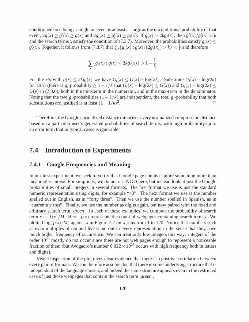
conditioned on it being a singleton event is at least as largeas the unconditional probability of thatevent, 2g(x)≥ g′(x) ≥ g(x) and 2gi(x) ≥ g′i(x) ≥ gi(x). If g(x) > 2kgi(x), theng′(x)/g′i(x) > kand the search termsx satisfy the condition of (7.3.7). Moreover, the probabilities satisfygi(x)≤g′i(x). Together, it follows from (7.3.7) that∑xgi(x) : g(x)/(2gi(x)) > k< 1
k and therefore
∑xgi(x) : g(x)≤ 2kgi(x)> 1− 1
k.
For thex’s with g(x) ≤ 2kgi(x) we haveGi(x) ≤ G(x) + log(2k). SubstituteGi(x)− log(2k)for G(x) (there isgi-probability≥ 1−1/k thatGi(x)− log(2k) ≤ G(x)) andGi(y)− log(2k) ≤G(y) in (7.3.6), both in the min-term in the numerator, and in the max-term in the denominator.Noting that the twogi-probabilities(1−1/k) are independent, the totalgi-probability that bothsubstitutions are justified is at least(1−1/k)2. 2
Therefore, the Google normalized distance minorizes everynormalized compression distancebased on a particular user’s generated probabilities of search terms, with high probability up toan error term that in typical cases is ignorable.
7.4 Introduction to Experiments
7.4.1 Google Frequencies and Meaning
In our first experiment, we seek to verify that Google page counts capture something more thanmeaningless noise. For simplicity, we do not use NGD here, but instead look at just the Googleprobabilities of small integers in several formats. The first format we use is just the standardnumeric representation using digits, for example “43”. Thenext format we use is the numberspelled out in English, as in “forty three”. Then we use the number spelled in Spanish, as in“cuarenta y tres”. Finally, we use the number as digits again, but now paired with the fixed andarbitrary search termgreen. In each of these examples, we compute the probability of searchterm x as f (x)/M. Here, f (x) represents the count of webpages containing search termx. Weplotted log( f (x)/M) againstx in Figure7.2 for x runs from 1 to 120. Notice that numbers suchas even multiples of ten and five stand out in every representation in the sense that they havemuch higher frequency of occurrence. We can treat only low integers this way: integers of theorder 1023 mostly do not occur since there are not web pages enough to represent a noticeablefraction of them (but Avogadro’s number 6.022×10²³ occurs with high frequency both in lettersand digits).
Visual inspection of the plot gives clear evidence that there is a positive correlation betweenevery pair of formats. We can therefore assume that that there is some underlying structure that isindependent of the language chosen, and indeed the same structure appears even in the restrictedcase of just those webpages that contain the search termgreen.
120
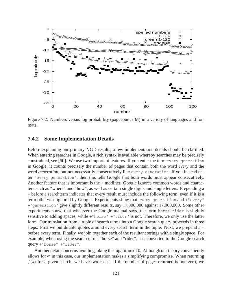
-35
-30
-25
-20
-15
-10
-5
0
0 20 40 60 80 100 120
log
prob
abilit
y
number
spelled numbers1-120
green 1-120spanish
Figure 7.2: Numbers versus log probability (pagecount / M) in a variety of languages and for-mats.
7.4.2 Some Implementation Details
Before explaining our primary NGD results, a few implementation details should be clarified.When entering searches in Google, a rich syntax is availablewhereby searches may be preciselyconstrained, see [50]. We use two important features. If you enter the termevery generationin Google, it counts precisely the number of pages that contain both the wordeveryand theword generation, but not necessarily consecutively likeevery generation. If you instead en-ter "every generation", then this tells Google that both words must appear consecutively.Another feature that is important is the+ modifier. Google ignores common words and charac-ters such as “where” and “how”, as well as certain single digits and single letters. Prepending a+ before a searchterm indicates that every result must include the following term, even if it is aterm otherwise ignored by Google. Experiments show thatevery generation and+"every"+"generation" give slightly different results, say 17,800,000 against 17,900,000. Some otherexperiments show, that whatever the Google manual says, theform horse rider is slightlysensitive to adding spaces, while+"horse" +"rider" is not. Therefore, we only use the latterform. Our translation from a tuple of search terms into a Google search query proceeds in threesteps: First we put double-quotes around every search term in the tuple. Next, we prepend a+before every term. Finally, we join together each of the resultant strings with a single space. Forexample, when using the search terms “horse” and “rider”, itis converted to the Google searchquery+"horse" +"rider".
Another detail concerns avoiding taking the logarithm of 0.Although our theory convenientlyallows for∞ in this case, our implementation makes a simplifying compromise. When returningf (x) for a given search, we have two cases. If the number of pages returned is non-zero, we
121
return twice this amount. If the pages is equal to 0, we do not return 0, but instead return 1.Thus, even though a page does not exist in the Google index, wecredit it half the probability ofthe smallest pages that do exist in Google. This greatly simplifies our implementation and seemsnot to result in much distortion in the cases we have investigated.
7.4.3 Three Applications of the Google Method
In this chapter we give three applications of the Google method: unsupervised learning in theform of hierarchical clustering, supervised learning using support vector machines, and match-ing using correlation. For the hierarchical clustering method we refer to Section4.1. and thecorrelation method is well known. For the supervised learning, several techniques are available.For the SVM method used in this thesis, we refer to the excellent exposition [16], and give abrief summary in Appendix5.3.3.
7.5 Hierarchical Clustering
For these examples, we used our software tool available fromhttp://complearn.sourceforge.net/,the same tool that has been used in other chapters to construct trees representing hierarchicalclusters of objects in an unsupervised way. However, now we use the normalized Google distance(NGD ) instead of the normalized compression distance (NCD ). Recapitulating, the methodworks by first calculating a distance matrix using NGD among all pairs of terms in the inputlist. Then it calculates a best-matching unrooted ternary tree using a novel quartet-method styleheuristic based on randomized hill-climbing using a new fitness objective function optimizingthe summed costs of all quartet topologies embedded in candidate trees.
7.5.1 Colors and Numbers
In the first example, the objects to be clustered are search terms consisting of the names of colors,numbers, and some tricky words. The program automatically organized the colors towards oneside of the tree and the numbers towards the other, Figure7.3. It arranges the terms which haveas only meaning a color or a number, and nothing else, on the farthest reach of the color side andthe number side, respectively. It puts the more general terms black and white, and zero, one, andtwo, towards the center, thus indicating their more ambiguous interpretation. Also, things whichwere not exactly colors or numbers are also put towards the center, like the word “small”. Wemay consider this an example of automatic ontology creation.
7.5.2 Dutch 17th Century Painters
In the example of Figure7.4, the names of fifteen paintings by Steen, Rembrandt, and Bol wereentered. The names of the associated painters were not included in the input, however they wereadded to the tree display afterword to demonstrate the separation according to painters. This typeof problem has attracted a great deal of attention [97]. A more classical solution is offered in
122

black
n8
white
n4
blue
n14
n13
n10
chartreuse
n6n7
purple
eight
n9
seven
n11
fiven15
four
n0
fortytwo
n2
green
n5
one
n16
n12
n3
orange
red
six
smalln18
n1
three
transparent
zero
two
n17
yellow
Figure 7.3: Colors and numbers arranged into a tree using NGD.
123
Steen Prince’s Day
Steen The Merry Family
Steen Leiden Baker Arend Oostwaert
Steen Keyzerswaert
Steen Woman at her Toilet
Steen Two Men Playing Backgammon
Rembrandt Hendrickje slapend
Rembrandt Portrait of Maria Trip
Rembrandt Portrait of Johannes Wtenbogaert
Rembrandt The Stone Bridge
Bol Maria Rey
Rembrandt The Prophetess Anna
Bol Consul Titus Manlius Torquatus
Bol Swartenhont
Bol Venus and Adonis
Figure 7.4: Fifteen paintings tree by three different painters arranged into a tree hierarchicalclustering. In the experiment, only painting title names were used; the painter prefix shown inthe diagram above was added afterwords as annotation to assist in interpretation. The paintersand paintings used follow.Rembrandt van Rijn : Hendrickje slapend; Portrait of Maria Trip;Portrait of Johannes Wtenbogaert ; The Stone Bridge ; The Prophetess Anna; Jan Steen :Leiden Baker Arend Oostwaert ; Keyzerswaert ; Two Men Playing Backgammon ; Woman at herToilet ; Prince’s Day ; The Merry Family; Ferdinand Bol : Maria Rey ; Consul Titus ManliusTorquatus ; Swartenhont ; Venus and Adonis.
[1], where a domain-specific database is used for similar ends.The present automatic obliviousmethod obtains results that compare favorably with the latter feature-driven method.
7.5.3 Chinese Names
In the example of Figure7.5, several Chinese names were entered. The tree shows the separationaccording to concepts like regions, political parties, people, etc. See Figure7.6 for Englishtranslations of these characters. This figure also shows a feature of the CompLearn system thathas not been encountered before: the CompLearn system can draw dotted lines with numbersinbetween each adjacent node along the perimeter of the tree. These numbers represent the NCDdistance between adjacent nodes in the final (ordered tree) output of the CompLearn system. Thetree is presented in such a way that the sum of these values in the entire ring is minimized. Thisgenerally results in trees that makes the most sense upon initial visual inspection, converting anunordered binary tree to an ordered one. This feature allowsfor a quick visual inspection aroundthe edges to determine the major groupings and divisions among coarse structured problems. Itgrew out of an idea originally suggested by Lloyd Rutledge atCWI [97].
124

Figure 7.5: Several people’s names, political parties, regions, and other Chinese names.125

!"#$
%&'((")"*"*
%&+,-.'(/"01!'(""0$
%&23'(
%24""4
%-4"'(/"01
5678""9
:;)"#
<=>?)/#
@A98
BCD:E)"#4"0
C:4""4
FG H/0I
JKLM#?I0#
NO"!"$
P:Q"0
R&'((""""*"*
STU/'#I#
V:W""0!""0'($
XYZW[
\]^_H#I`
abc"4deef"
Figure 7.6: English Translation of Chinese Names
126
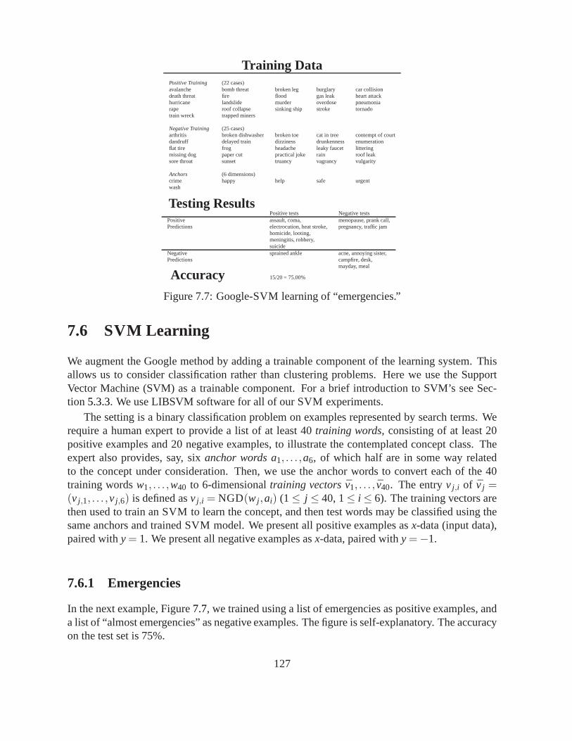
Training DataPositive Training (22 cases)avalanche bomb threat broken leg burglary car collisiondeath threat fire flood gas leak heart attackhurricane landslide murder overdose pneumoniarape roof collapse sinking ship stroke tornadotrain wreck trapped miners
Negative Training (25 cases)arthritis broken dishwasher broken toe cat in tree contemptof courtdandruff delayed train dizziness drunkenness enumerationflat tire frog headache leaky faucet litteringmissing dog paper cut practical joke rain roof leaksore throat sunset truancy vagrancy vulgarity
Anchors (6 dimensions)crime happy help safe urgentwash
Testing ResultsPositive tests Negative tests
Positive assault, coma, menopause, prank call,Predictions electrocution, heat stroke, pregnancy, traffic jam
homicide, looting,meningitis, robbery,suicide
Negative sprained ankle acne, annoying sister,Predictions campfire, desk,
mayday, meal
Accuracy 15/20 = 75.00%
Figure 7.7: Google-SVM learning of “emergencies.”
7.6 SVM Learning
We augment the Google method by adding a trainable componentof the learning system. Thisallows us to consider classification rather than clusteringproblems. Here we use the SupportVector Machine (SVM) as a trainable component. For a brief introduction to SVM’s see Sec-tion 5.3.3. We use LIBSVM software for all of our SVM experiments.
The setting is a binary classification problem on examples represented by search terms. Werequire a human expert to provide a list of at least 40training words, consisting of at least 20positive examples and 20 negative examples, to illustrate the contemplated concept class. Theexpert also provides, say, sixanchor words a1, . . . ,a6, of which half are in some way relatedto the concept under consideration. Then, we use the anchor words to convert each of the 40training wordsw1, . . . ,w40 to 6-dimensionaltraining vectorsv1, . . . , v40. The entryv j ,i of v j =(v j ,1, . . . ,v j ,6) is defined asv j ,i = NGD(w j ,ai) (1≤ j ≤ 40, 1≤ i ≤ 6). The training vectors arethen used to train an SVM to learn the concept, and then test words may be classified using thesame anchors and trained SVM model. We present all positive examples asx-data (input data),paired withy = 1. We present all negative examples asx-data, paired withy =−1.
7.6.1 Emergencies
In the next example, Figure7.7, we trained using a list of emergencies as positive examples, anda list of “almost emergencies” as negative examples. The figure is self-explanatory. The accuracyon the test set is 75%.
127
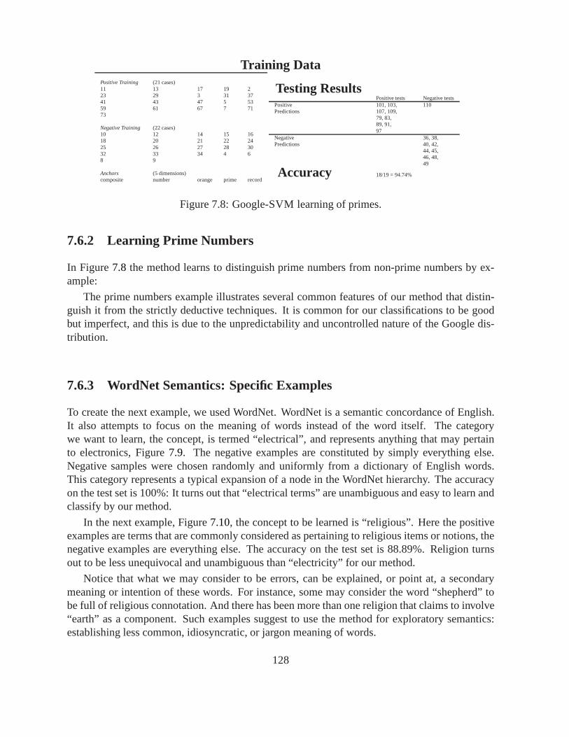
Training DataPositive Training (21 cases)11 13 17 19 223 29 3 31 3741 43 47 5 5359 61 67 7 7173
Negative Training (22 cases)10 12 14 15 1618 20 21 22 2425 26 27 28 3032 33 34 4 68 9
Anchors (5 dimensions)composite number orange prime record
Testing ResultsPositive tests Negative tests
Positive 101, 103, 110Predictions 107, 109,
79, 83,89, 91,97
Negative 36, 38,Predictions 40, 42,
44, 45,46, 48,49
Accuracy 18/19 = 94.74%
Figure 7.8: Google-SVM learning of primes.
7.6.2 Learning Prime Numbers
In Figure7.8 the method learns to distinguish prime numbers from non-prime numbers by ex-ample:
The prime numbers example illustrates several common features of our method that distin-guish it from the strictly deductive techniques. It is common for our classifications to be goodbut imperfect, and this is due to the unpredictability and uncontrolled nature of the Google dis-tribution.
7.6.3 WordNet Semantics: Specific Examples
To create the next example, we used WordNet. WordNet is a semantic concordance of English.It also attempts to focus on the meaning of words instead of the word itself. The categorywe want to learn, the concept, is termed “electrical”, and represents anything that may pertainto electronics, Figure7.9. The negative examples are constituted by simply everything else.Negative samples were chosen randomly and uniformly from a dictionary of English words.This category represents a typical expansion of a node in theWordNet hierarchy. The accuracyon the test set is 100%: It turns out that “electrical terms” are unambiguous and easy to learn andclassify by our method.
In the next example, Figure7.10, the concept to be learned is “religious”. Here the positiveexamples are terms that are commonly considered as pertaining to religious items or notions, thenegative examples are everything else. The accuracy on the test set is 88.89%. Religion turnsout to be less unequivocal and unambiguous than “electricity” for our method.
Notice that what we may consider to be errors, can be explained, or point at, a secondarymeaning or intention of these words. For instance, some may consider the word “shepherd” tobe full of religious connotation. And there has been more than one religion that claims to involve“earth” as a component. Such examples suggest to use the method for exploratory semantics:establishing less common, idiosyncratic, or jargon meaning of words.
128
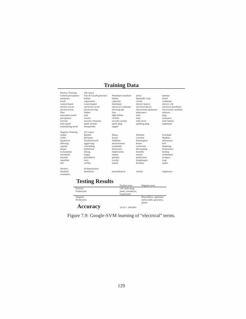
Training DataPositive Training (58 cases)Cottrell precipitator Van de Graaff generator Wimshurst machine aerial antennaattenuator ballast battery bimetallic strip boardbrush capacitance capacitor circuit condensercontrol board control panel distributer electric battery electric cellelectric circuit electrical circuit electrical condenser electrical device electrical distributorelectrical fuse electrical relay electrograph electrostatic generator electrostatic machinefilter flasher fuse inductance inductorinstrument panel jack light ballast load plugprecipitator reactor rectifier relay resistancesecurity security measures security system solar array solar batterysolar panel spark arrester spark plug sparking plug suppressertransmitting aerial transponder zapper
Negative Training (55 cases)Andes Burnett Diana DuPonts FrieslandGibbs Hickman Icarus Lorraine MadeiraQuakeress Southernwood Waltham Washington adventuresaffecting aggrieving attractiveness bearer bollcapitals concluding constantly conviction dammingdeeper definitions dimension discounting distinctnessexclamation faking helplessness humidly hurlingintroduces kappa maims marine moderatelymonster parenthesis pinches predication prospectrepudiate retry royalty shopkeepers soapsob swifter teared thrashes tuples
Anchors (6 dimensions)bumbled distributor premeditation resistor suppressorswimmers
Testing ResultsPositive tests Negative tests
Positive cell, male plug,Predictions panel, transducer,
transformerNegative Boswellizes, appointer,Predictions enforceable, greatness,
planet
Accuracy 10/10 = 100.00%
Figure 7.9: Google-SVM learning of “electrical” terms.
129

Training DataPositive Training (22 cases)Allah Catholic Christian Dalai Lama GodJerry Falwell Jesus John the Baptist Mother Theresa MuhammadSaint Jude The Pope Zeus bible churchcrucifix devout holy prayer rabbireligion sacred
Negative Training (23 cases)Abraham Lincoln Ben Franklin Bill Clinton Einstein George WashingtonJimmy Carter John Kennedy Michael Moore atheist dictionaryencyclopedia evolution helmet internet materialisticminus money mouse science secularseven telephone walking
Anchors (6 dimensions)evil follower history rational scripturespirit
Testing ResultsPositive tests Negative tests
Positive altar, blessing, earth, shepherdPredictions communion, heaven,
sacrament, testament,vatican
Negative angel Aristotle, Bertrand Russell,Predictions Greenspan, John,
Newton, Nietzsche,Plato, Socrates,air, bicycle,car, fire,five, man,monitor, water,whistle
Accuracy 24/27 = 88.89%
Figure 7.10: Google-SVM learning of “religious” terms.
7.6.4 WordNet Semantics: Statistics
The previous examples show only a few hand-crafted special cases. To investigate the moregeneral statistics, a method was devised to estimate how well the NGD -Google-SVM approachagrees with WordNet in a large number of automatically selected semantic categories. Eachautomatically generated category followed the following sequence.
First we must review the structure of WordNet; the followingis paraphrased from the officialWordNet documentation available online. WordNet is calleda semantic concordance of theEnglish language. It seeks to classify words into many categories and interrelate the meaningsof those words. WordNet contains synsets. A synset is a synonym set; a set of words that areinterchangeable in some context, because they share a commonly-agreed upon meaning withlittle or no variation. Each word in English may have many different senses in which it may beinterpreted; each of these distinct senses points to a different synset. Every word in WordNethas a pointer to at least one synset. Each synset, in turn, must point to at least one word. Thus,we have a many-to-many mapping between English words and synsets at the lowest level ofWordNet. It is useful to think of synsets as nodes in a graph. At the next level we have lexicaland semantic pointers. Lexical pointers are not investigated in this thesis; only the followingsemantic pointer types are used in our comparison: A semantic pointer is simply a directed edgein the graph whose nodes are synsets. The pointer has one end we call asourceand the other endwe call adestination. The following relations are used:
1. hyponym: X is a hyponym of Y if X is a (kind of) Y.
130
2. part meronym: X is a part meronym of Y if X is a part of Y.
3. member meronym: X is a member meronym of Y if X is a member of Y.
4. attribute : A noun synset for which adjectives express values. The nounweight is anattribute, for which the adjectiveslight andheavyexpress values.
5. similar to : A synset is similar to another one if the two synsets have meanings that aresubstantially similar to each other.
Using these semantic pointers we may extract simple categories for testing. First, a randomsemantic pointer (or edge) of one of the types above is chosenfrom the WordNet database. Next,the source synset node of this pointer is used as a sort of root. Finally, we traverse outward in abreadth-first order starting at this node and following onlyedges that have an identical semanticpointer type; that is, if the original semantic pointer was ahyponym, then we would only followhyponym pointers in constructing the category. Thus, if we were to pick a hyponym link initiallythat says atiger is acat, we may then continue to follow further hyponym relationships in orderto continue to get more specific types of cats. See the WordNethomepage [37] documentationfor specific definitions of these technical terms. For examples of each of these categories consultthe experiments listed in the Appendix at [23].
Once a category is determined, it is expanded in a breadth first way until at least 38 synsetsare within the category. 38 was chosen to allow a reasonable amount of training data to bepresented with several anchor dimensions, yet also avoiding too many. Here,Bernie’s Rule1
is helpful: it states that the number of dimensions in the input data must not exceed one tenththe number of training samples. If the category cannot be expanded this far, then a new one ischosen. Once a suitable category is found, and a set of at least 38 members has been formed, atraining set is created using 25 of these cases, randomly chosen. Next, three are chosen randomlyas anchors. And finally the remaining ten are saved as positive test cases. To fill in the negativetraining cases, random words are chosen from the WordNet database. Next, three random wordsare chosen as unrelated anchors. Finally, 10 random words are chosen as negative test cases.
For each case, the SVM is trained on the training samples, converted to 6-dimensional vec-tors using NGD . The SVM is trained on a total of 50 samples. Thekernel-width and error-costparameters are automatically determined using five-fold cross validation. Finally testing is per-formed using 20 examples in a balanced ensemble to yield a final accuracy.
There are several caveats with this analysis. It is necessarily rough, because the problemdomain is difficult to define. There is no protection against certain randomly chosen negativewords being accidentally members of the category in question, either explicitly in the greaterdepth transitive closure of the category, or perhaps implicitly in common usage but not indicatedin WordNet. In several cases, such as “radio wave” and “DC” inthe “big science” experiment,there appears to be an arguable case to support the computer’s classification in cases where thisphenomenon occurs. Another detail to notice is that WordNetis available through some webpages, and so undoubtedly contributes something to Google pagecounts. Further experiments
1Allegedly named after Bernie Widrow in the context of neuralnetwork training.
131
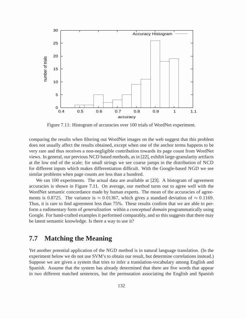
0
5
10
15
20
25
30
0.4 0.5 0.6 0.7 0.8 0.9 1 1.1
num
ber o
f tria
ls
accuracy
Accuracy Histogram
Figure 7.11: Histogram of accuracies over 100 trials of WordNet experiment.
comparing the results when filtering out WordNet images on the web suggest that this problemdoes not usually affect the results obtained, except when one of the anchor terms happens to bevery rare and thus receives a non-negligible contribution towards its page count from WordNetviews. In general, our previous NCD based methods, as in [22], exhibit large-granularity artifactsat the low end of the scale; for small strings we see coarse jumps in the distribution of NCDfor different inputs which makes differentiation difficult. With the Google-based NGD we seesimilar problems when page counts are less than a hundred.
We ran 100 experiments. The actual data are available at [23]. A histogram of agreementaccuracies is shown in Figure7.11. On average, our method turns out to agree well with theWordNet semantic concordance made by human experts. The mean of the accuracies of agree-ments is 0.8725. The variance is≈ 0.01367, which gives a standard deviation of≈ 0.1169.Thus, it is rare to find agreement less than 75%. These resultsconfirm that we are able to per-form a rudimentary form ofgeneralizationwithin aconceptual domainprogrammatically usingGoogle. For hand-crafted examples it performed comparably, and so this suggests that there maybe latent semantic knowledge. Is there a way to use it?
7.7 Matching the Meaning
Yet another potential application of the NGD method is in natural language translation. (In theexperiment below we do not use SVM’s to obtain our result, butdetermine correlations instead.)Suppose we are given a system that tries to infer a translation-vocabulary among English andSpanish. Assume that the system has already determined thatthere are five words that appearin two different matched sentences, but the permutation associating the English and Spanish
132
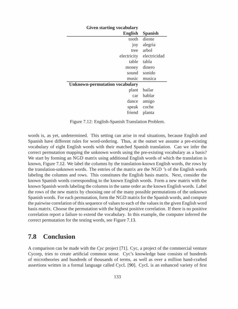
Given starting vocabularyEnglish Spanish
tooth dientejoy alegriatree arbol
electricity electricidadtable tabla
money dinerosound sonidomusic musica
Unknown-permutation vocabularyplant bailar
car hablardance amigospeak cochefriend planta
Figure 7.12: English-Spanish Translation Problem.
words is, as yet, undetermined. This setting can arise in real situations, because English andSpanish have different rules for word-ordering. Thus, at the outset we assume a pre-existingvocabulary of eight English words with their matched Spanish translation. Can we infer thecorrect permutation mapping the unknown words using the pre-existing vocabulary as a basis?We start by forming an NGD matrix using additional English words of which the translation isknown, Figure7.12. We label the columns by the translation-known English words, the rows bythe translation-unknown words. The entries of the matrix are the NGD ’s of the English wordslabeling the columns and rows. This constitutes the Englishbasis matrix. Next, consider theknown Spanish words corresponding to the known English words. Form a new matrix with theknown Spanish words labeling the columns in the same order asthe known English words. Labelthe rows of the new matrix by choosing one of the many possiblepermutations of the unknownSpanish words. For each permutation, form the NGD matrix forthe Spanish words, and computethe pairwise correlation of this sequence of values to each of the values in the given English wordbasis matrix. Choose the permutation with the highest positive correlation. If there is no positivecorrelation report a failure to extend the vocabulary. In this example, the computer inferred thecorrect permutation for the testing words, see Figure7.13.
7.8 Conclusion
A comparison can be made with theCycproject [71]. Cyc, a project of the commercial ventureCycorp, tries to create artificial common sense. Cyc’s knowledge base consists of hundredsof microtheories and hundreds of thousands of terms, as wellas over a million hand-craftedassertions written in a formal language called CycL [90]. CycL is an enhanced variety of first
133

Predicted (optimal) permutation
English Spanishplant planta
car cochedance bailarspeak hablarfriend amigo
Figure 7.13: Translation Using NGD.
order predicate logic. This knowledge base was created overthe course of decades by paidhuman experts. It is therefore of extremely high quality. Google, on the other hand, is almostcompletely unstructured, and offers only a primitive querycapability that is not nearly flexibleenough to represent formal deduction. But what it lacks in expressiveness Google makes up forin size; Google has already indexed more than eight billion pages and shows no signs of slowingdown.
Epistemology: In the case of context-free statistical compression such asgzip , we are tryingto approximate the Kolmogorov complexity of a string. Another way of describing the calcu-lation is to view it as determining a probability mass function (viewing the compressed stringas Shannon-Fano code, Section2.7), approximating theuniversal distribution, that is, the nega-tive exponential of the Kolmogorov complexity [79]. The universal probability of a given stringcan equivalently be defined as the probability that the reference universal Turing machine out-puts the string if its input program is generated by fair coinflips. In a similar manner, we canassociate a particular Shannon-Fano code, theGoogle code, with the Google probability massfunction. Coding every search term by its Google code, we define a “Google compressor.” Then,in the spirit of Section7.3, we can view the Google probability mass function as a universal dis-tribution for the individual Google probability mass functions generated by the individual webauthors, substituting “web authors” for “Turing machines”.
Concerning the SVM method: The Google-SVM method does not use an individual word inisolation, but instead uses an ordered list of its NGD relationships with fixed anchors. This thenremoves the possibility of attaching to the isolated (context-free) interpretation of a literal term.That is to say, the inputs to our SVM are not directly search terms, but instead an image of thesearch term through the lens of the Google distribution, andrelative to other fixed terms whichserve as a grounding for the term. In most schools of ontological thought, and indeed in theWordNet database, there is imagined a two-level structure that characterizes language: a many-to-many relationship between word-forms or utterances andtheir many possible meanings. Eachlink in this association will be represented in the Google distribution with strength proportionalto how common that usage is found on the web. The NGD then amplifies and separates themany contributions towards the aggregate page count sum, thereby revealing some componentsof the latent semantic web. In almost every informal theory of cognition we have the idea ofconnectedness of different concepts in a network, and this is precisely the structure that our
134
experiments attempt to explore.
Universality: The Google distribution is a comparable notion, in the context of the world-wide-web background information, to the universal distribution: The universal distribution mul-tiplicatively dominates all other distributions in that itassigns a higher weight to some elementswhen appropriately scaled. This suggests that it covers everything without bound. Google surelyrepresents the largest publicly-available single corpus of aggregate statistical and indexing in-formation so far created. Only now has it been cheap enough tocollect this vast quantity ofdata, and it seems that even rudimentary analysis of this distribution yields a variety of intriguingpossibilities. One of the simplest avenues for further exploration must be to increase trainingsample size, because it is well-known that SVM accuracy increases with training sample size.It is likely that this approach can never achieve 100% accuracy like in principle deductive logiccan, because the Google distribution mirrors humankind’s own imperfect and varied nature. Butit is also clear that in practical terms the NGD can offer an easy way to provide results that aregood enough for many applications, and which would be far toomuch work if not impossible toprogram in a foolproof deductive way.
The Road Ahead: We have demonstrated that NGD can be used to extract meaning in a varietyof ways from the statistics inherent to the Google database.So far, all of our techniques lookonly at the page count portion of the Google result sets and achieve surprising results. How muchmore amazing might it be when the actual contents of search results are analyzed? Consider thepossibility of using WordNet familiarity counts to filter returned search results to select only theleast familiar words, and then using these in turn as furtherinputs to NGD to create automaticdiscourse or concept diagrams with arbitrary extension. Orperhaps this combination can be usedto expand existing ontologies that are only seeded by humans. Let us list some of the futuredirections and potential application areas:
1. There seems to also be an opportunity to apply these techniques to generic language acqui-sition, word sense disambiguation, knowledge representation, content-filtration and collab-orative filtering, chat bots, and discourse generation.
2. There are potential applications of this technique to semi-intelligent user-interface design;for predictive completion on small devices, speech recognition, or handwriting recognition.
3. A user interface possibility is the idea of concept-classprogramming for non-programmers,or software to form a conceptual predicate by way of example without forcing the user tolearn a formal programming language. This might be used, forexample, in a networkcontent filtration system that is installed by non-programmer parents to protect their youngchildren from some parts of the internet. Or perhaps an IT manager is able to adjust therule determining if a particular email message is a well-known virus and should be filteredwithout writing explicit rules but just showing some examples.
135
4. How many people are able to write down a list of prime numbers as shown in an earlier testcase, Figure7.8, compared to how many people are able to write a program in a real pro-gramming language that can calculate prime numbers? Concept clustering by example issignificantly simpler than any formal programming languageand often yields remarkablyaccurate results without any effort at hand-tuning parameters.
5. The colors versus numbers tree example, Figure7.3, is rife with possibilities. A majorchallenge of the Semantic Web and XML as it stands is in integrating diverse ontologiescreated by independent entities [67]. XML makes the promise of allowing seamless inte-gration of web services via customized structured tags. This promise is for the most partunrealized at this point on the web, however, because there is not yet sufficient agreementon what sets of XML tags to use in order to present information; when two different partieseach build databases of recipes, but one organizes the recipes according to their countryof origin and another according to their sweetness or savoryflavor, these two databasescannot “understand” one another insofar as they may exchange recipes. XML allows usto format our data in a structured way, but fails to provide for a way for different struc-ture conventions to interoperate. There have been many attempts to solve this and nonehave been satisfactory. Usually solutions involve mappingthe separate schemas into somesort of global schema and then creating a global standardization problem that requires sig-nificant coordinated effort to solve. Another approach is tocreate a meta-language likeDAML that allows for automatic translation among certain very similar types of ontolo-gies, however this requires a great deal of effort and forethought on the part of the schemadesigners in advance and is brittle in the face of changing ontologies. By using NGD wemay create a democratic and natural ontology for almost any application in an unsuper-vised way. Furthermore, if instead we want finer control overthe ontological organization,then a human expert may define a custom ontology and then NGD may be used to pro-vide a normal, global, and automatic reference frame withinwhich this ontology may beunderstood without additional costly human effort. So, forexample, NGD may be usedin the recipe example above, Figure7.12, 7.13, to automatically “understand” the differ-ence between a Chinese or Mediterranean recipe, and could thus be used to automaticallytranslate between the two conflicting ontologies.
6. Another future direction is to apply multiple concurrentbinary classifiers for the sameclassification problem but using different anchors. The separate classifications would haveto be combined using a voting scheme, boosting scheme, or other protocol in an effort toboost accuracy.
This section owes thanks to Teemu Roos, Hannes Wettig, PetriMylliymaki, and Henry Tirriat COSCO and The Helsinki Institute for Information Technology for interesting discussions. Wealso thank Chih-Jen Lin and his excellent group for providing and supporting vigorously, free ofcharge to all, the very easy to use LIBSVM package. We thank the Cognitive Science Laboratoryat Princeton University for providing the wonderful and free WordNet database. And we wish tothank the staff of Google, Inc. for their delightful supportof this research by providing an APIas well as generous access to their websearch system.
136

Chapter 8
Stemmatology
Stemmatology studies relations among different variants of a text that has been gradually alteredas a result of imperfectly copying the text over and over again. This chapter presents a newmethod for using this assumption to reconstruct a lineage tree explicating the derivational rela-tionships among the many variations, just as we might reconstruct an evolutionary tree from a setof gene sequences. We propose a new computer assisted methodfor stemmatic analysis basedon compression of the variants. We will provide an overview of the chapter at the end of the nextsection. The method is related to phylogenetic reconstruction criteria such as maximum parsi-mony and maximum likelihood. We apply our method to the tradition of the legend of St. Henryof Finland, and report encouraging preliminary results. The obtained family tree of the variants,the stemma, corresponds to a large extent with results obtained with more traditional methods.Some of the identified groups of manuscripts are previously unrecognized ones. Moreover, dueto the impossibility of manually exploring all plausible alternatives among the vast number ofpossible trees, this work is the first attempt at a complete stemma for the legend of St. Henry.The used methods are being released as open-source software, and are entirely distinct from theCompLearn system. They are presented here only for rough comparison.
8.1 Introduction
St. Henry, according to the medieval tradition Bishop of Uppsala (Sweden) and the first Bishopof Finland, is the key figure of the Finnish Middle Ages. He seems to have been one of the leadersof a Swedish expedition to Finland probably around 1155. After this expedition Henry stayed inFinland with sad consequences: he was murdered already nextyear. He soon became the patronsaint of Turku cathedral and of the bishopric covering the whole of Finland. He remained theonly ‘local’ one of the most important saints until the reformation. Henry is still considered tobe the Finnish national saint. The knowledge of writing was almost totally concentrated into thehands of the Church and the clergymen during the early and high Middle Ages. On the otherhand, the official and proper veneration of a saint needed unavoidably a written text containingthe highlights of the saint’s life and an account of his miracles to be recited during the servicesin the church. The oldest text concerning St. Henry is his legend written in Latin. It contains
137
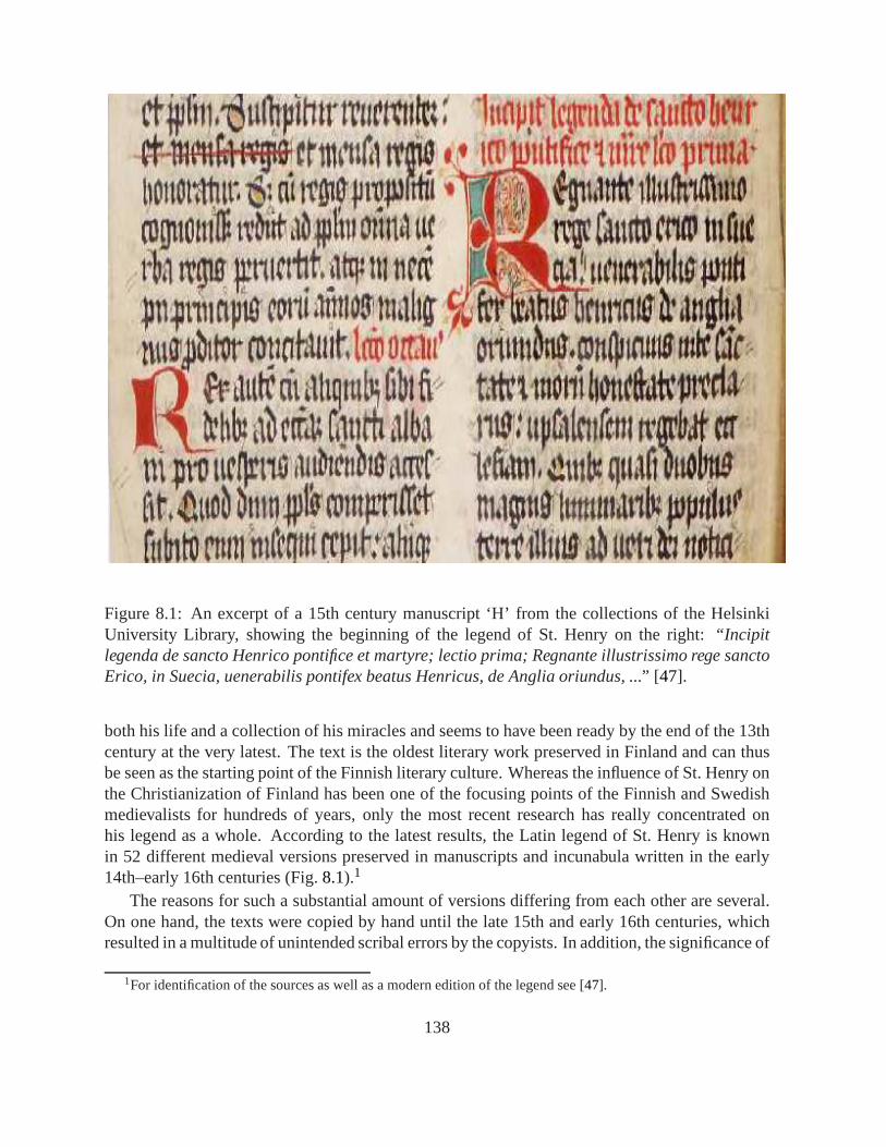
Figure 8.1: An excerpt of a 15th century manuscript ‘H’ from the collections of the HelsinkiUniversity Library, showing the beginning of the legend of St. Henry on the right:“Incipitlegenda de sancto Henrico pontifice et martyre; lectio prima; Regnante illustrissimo rege sanctoErico, in Suecia, uenerabilis pontifex beatus Henricus, deAnglia oriundus, ...”[47].
both his life and a collection of his miracles and seems to have been ready by the end of the 13thcentury at the very latest. The text is the oldest literary work preserved in Finland and can thusbe seen as the starting point of the Finnish literary culture. Whereas the influence of St. Henry onthe Christianization of Finland has been one of the focusingpoints of the Finnish and Swedishmedievalists for hundreds of years, only the most recent research has really concentrated onhis legend as a whole. According to the latest results, the Latin legend of St. Henry is knownin 52 different medieval versions preserved in manuscriptsand incunabula written in the early14th–early 16th centuries (Fig.8.1).1
The reasons for such a substantial amount of versions differing from each other are several.On one hand, the texts were copied by hand until the late 15th and early 16th centuries, whichresulted in a multitude of unintended scribal errors by the copyists. In addition, the significance of
1For identification of the sources as well as a modern edition of the legend see [47].
138
the cult of St. Henry varied considerably from one part of theLatin Christendom to the other. Inthe medieval bishopric of Turku covering the whole of medieval Finland St. Henry was veneratedas the most important local saint, whose adoration requiredthe reciting of the whole legendduring the celebrations of the saint’s day. In Sweden, for instance, St. Henry was not so importanta saint, which led to different kinds of abridgments fitted into the needs of local bishoprics andparishes. As a consequence, the preserved versions of the legend are all unique.
With the aid of traditional historically oriented auxiliary sciences like codicology and pa-leography it is possible to find out — at least roughly — where and when every version waswritten. Thus, the versions form a pattern representing themedieval and later dissemination ofthe text. Even if the existent manuscripts containing the different versions represent but a tinypart of the much larger number of manuscripts and versions written during the Middle Ages, theystill provide us with an insight into a variety of aspects of medieval culture. The versions help toreconstruct the actual writing process and the cultural ties that carried the text from one place toanother. When one combines the stemma — i.e. the family tree —of a text with a geographicalmap and adds the time dimension, one gets important information that no single historical sourcecan ever provide a historian with. The potential of this kindof an approach is emphasized whenresearching hagiographical texts — i.e. saints’ lives, forinstance — since they were the mosteagerly read and most vastly disseminated literary genre ofthe Middle Ages.
Taking into consideration the possibilities of stemmatology, it is not surprising that the histo-rians and philologists have tried to establish a reliable way to reconstruct the stemma of the textand its versions for centuries. The main difficulty has been the great multitude of textual variantsthat have to be taken into consideration at the same time. An example from the legend materialof St. Henry shall elucidate the problems: there are over 50 manuscripts and incunabula to betaken into consideration; in the relatively short text there are nearly one thousand places wherethe versions differ from each other. Since the multitude of variants rises easily to tens of thou-sands, it has been impossible for researchers using traditional methods of paper and pen to formthe stemma and thus get reliable answers to the questions related to the writing and disseminat-ing of the text. There have been some previous attempts to solve the problems of stemmatologywith the aid of computer science. In addition, the powerful computer programs developed forthe needs of the computer aided cladistics in the field of evolutionary biology have been used. Inmany cases this has proven to be a fruitful approach, extending the possibilities of stemmaticsto the analysis of more complex textual traditions that are outside the reach of manual analysis.Moreover, formalizing the often informal and subjective methods used in manual analysis makesthe methods and results obtained with them more transparentand brings them under objectivescrutiny. Still, many issues in computer assisted stemmatic analysis remain unsolved, underlin-ing the importance of advances towards general and reliablemethods for shaping the stemma ofa text.
Overview of this Chapter: The chapter is organized as follows: In Section8.2 we presenta criterion for stemmatic analysis that is based on compression of the manuscripts. We thenoutline an algorithm, in Section8.3, that builds stemmata by comparing a large number of tree-shaped stemmata and choosing the one that minimizes the criterion. The method is demonstratedon a simple example in Section8.4, where we also present our main experiment using some50 variants of the legend of St. Henry, and discuss some of therestrictions of the method and
139
potential ways to overcome them. Conclusions are presentedin Section8.5. We also compareour method to a related method in the CompLearn package in Appendix A.
8.2 A Minimum-Information Criterion
One of the most applied methods in biological phylogeny is so-called maximum parsimony.A maximally parsimonious tree minimizes the total number ofdifferences between connectednodes — i.e., species, individuals, or manuscripts that aredirectly related — possibly weightedby their importance. Stemmatology analysis is based on variable readings that result from un-intentional errors in copying or intentional omissions, insertions, or other modifications. In hisseminal work on computer assisted stemmatology, O’Hara used a parsimony method of the PAUPsoftware [110] in Robinson’s Textual Criticism challenge [93]. For further applications of maxi-mum parsimony and related method, see [49, 69, 107, 117] and references therein.
The compression-basedminimum informationcriterion shares many properties of the verypopular maximum parsimony method. Both can also be seen as instances of theminimum de-scription length(MDL) principle of Rissanen [91] — although this is slightly anachronistic: themaximum parsimony method predates the more general MDL principle — which in turn is aformal version of Occam’s razor. The underlying idea in the minimum information criterion is tominimize the amount of information, orcode-length, required to reproduce all the manuscriptsby the process of copying and modifying the text under study.In order to describe a new ver-sion of an existing manuscript, one needs an amount of information that depends on both theamount and the type of modifications made. For instance, a deletion of a word or a change ofword order requires less information to describe compared to introducing a completely new ex-pression. In order to be concrete, we need a precise, numerical, and computable measure forthe amount of information. The commonly accepted definitionof the amount information inindividual objects is Kolmogorov complexity [57, 79], defined as the length of the shortest com-puter program to describe the given object, as explained in Chapter 3. However, Kolmogorovcomplexity is defined only up to a constant that depends on thelanguage used to encode pro-grams, and what is more, fundamentally uncomputable. In thespirit of a number of earlierauthors [7, 10, 20, 22, 45, 82, 115] we approximate Kolmogorov complexity by using a com-pression program, also as we did in previous chapters. Currently, we usegzip based on theLZ77 [122] algorithm, and plan to experiment with other compressors in subsequent work. Inparticular, given two strings,x andy, the amount of information iny conditional onx, denotedbyC(y | x) is given by the length of the compressed version of the concatenated stringx,y minusthe length of the compressed version ofx alone2. A simple example illustrating these conceptsis given below in Section8.4.
In addition to the MDL interpretation, our method can be seenas (an approximation of)maximum likelihood, another commonly used criterion in phylogeny. The maximum likelihoodcriterion requires that we have a probabilistic model for evolution, assigning specific probabilitiesfor each kind of change. The joint likelihood of the whole graph is then evaluated as a product
2We insert a newline in the end of each string and betweenx andy.
140
of likelihoods of the individual changes. The tree achieving the highest joint likelihood giventhe observed data is then preferred. In the case of manuscripts such a model is clearly moredifficult to construct that in biology, where the probabilities of mutation can be estimated fromexperimental data. Nevertheless, a model for manuscript evolution is presented in [106]. Code-length is isomorphic to (behaves in the same way as) likelihood: sums of code-lengths have adirect correspondence with products of likelihoods. If theprobability induced by the informationcost, 2−C(y|x), is approximately proportional to the likelihood of creating a copyy based on theoriginalx, then minimizing the total information cost approximates maximizing the likelihood.
Let G = (V,E) be an undirected graph whereV is a set of nodes corresponding to the textvariants,E ⊂V×V is a set of edges. We require that the graph is a connected bifurcating tree,i.e., that (i) each node has either one or three neighbors, and (ii) the tree is acyclic. Such a graphG can be made directed by picking any one of the nodes as a root and directing each edge awayfrom the root. Given a directed graph~G, the total information cost of the tree is given by
C(~G) = ∑v∈V
C(v | Pa(v))
= ∑v∈V
C(Pa(v),v)−C(Pa(v)), (8.2.1)
where Pa(v) denotes the parent node ofv unlessv is the root in which case Pa(v) is the emptystring. Assuming that order has no significant effect on the complexity of a concatenated string,i.e., we haveC(x,y)≈C(y,x), as seems to be the case in our data, it can easily verified thatforacyclic bifurcating trees, the above can rewritten as
C(G)≈ ∑(v,w)∈E
C(v,w)−2 ∑v∈VI
C(v), (8.2.2)
where the first summation has a term for each edge in the graph,and the second summation goesover the set of interior nodesVI . The formula is a function of the undirected structureG only:the choice of the root is irrelevant. The factor two in the latter term comes from usingbifurcatingtrees.
For practical reasons we make three modifications to this criterion. First, as we explain inthe next section, due to algorithmic reasons we need to splice the texts in smaller segments, notlonger than roughly 10–20 words (we used 11). Secondly, we found that the cost assigned bygzip to reproducing an identical copy of a string is too high in thesense that it is sometimes‘cheaper’ to omit a large part of the text for a number of generations and to re-invent it later in anidentical form. Therefore we define the cost of making an identical copy to be zero. Thirdly, it isknown that the variation between an ampersand (’&’) and the wordet, and the lettersv andu wasmostly dependent on the style of the copyist and changed withtime and region, and thus, bearslittle information relevant to stemmatic analysis. This domain knowledge was taken into accountby replacing, in both of the above cases, all occurrences of the former by the latter3. Thus, we
3Howeet al. [49] use as an example the wordskirk andchurchin 15th century English whose variation mainlyreflects local dialect.
141
use the following modified cost function
C′(~G) = ∑v∈V
n
∑i=1
C′(vi | Pai(v)), (8.2.3)
wheren is the number of segments into which each text is spliced,vi and Pai(v) are theithsegment of variantv and its parent, respectively, all strings are modified according to the aboverules (ampersand toet, andv to u), andC′(x | y) equals thegzip cost if x and y differ, andzero otherwise. This modified cost also allows a form similarto (8.2.2) and hence, is practicallyindependent of the choice of the root.
8.3 An Algorithm for Constructing Stemmata
Since it is known that many of the text variants have been lostduring the centuries betweenthe time of the writing of the first versions and present time,it is not realistic to build a tree ofonly the about 50 variants that we have as our data. This problem is even more prominent inbiology where we can only make observations about organismsthat still exist (excluding fossilevidence). The common way of handling this problem is to include in the tree a number of‘hidden’ nodes, i.e., nodes representing individuals whose characteristics are unobserved. Weconstruct bifurcating trees that haveN observed nodes as leafs, andN−2 hidden nodes as theinterior nodes.
Evaluating the criterion (8.2.3) now involves the problem of dealing with the hidden nodes.Without knowing the values of Pai(v), it is not possible to computeC′(v | Pai(v)). We solve thisproblem by searching simultaneously for the best tree structure~G and for the optimal contents ofthe hidden nodes with respect to criterion (8.2.3). As mentioned above, we patch up the contentsof the interior nodes from segments of length 10–20 words appearing in some of the availablevariants. In principle we would like to do this on a per-word-basis, which would not be a notablerestriction since it is indeed reasonable to expect that a reconstruction only consists of wordsappearing in the available variants — any other kind of behavior would require rather strikinginnovation. However, since we evaluate thegzip cost in terms of the segments, it is likely givebetter values when the segments are longer than one word. Secondly, one of the most commonmodifications is change in word order. Using 10-20 word segments we assign less cost to changein word order than to genuine change of words, unless the change happens to cross a segmentborder.
Perhaps surprisingly, given a tree structure, finding the optimal contents is feasible. Themethod for efficiently optimizing the contents of the hiddennodes is an instance of dynamicprogramming and called ‘the Sankoff algorithm’ [40] or ‘the Felsenstein’s algorithm’ [104]. AsSiepel and Haussler [104] note, it is in fact an instance of a ‘message-passing’ or ‘elimination’algorithm in graphical models (see also [42]). The basic idea is to maintain for each node a tableof minimal costs for the whole subtree starting at the node, given that the contents of the nodetake any given value. For instance, let us fix a segment, and denote byx1, . . . ,xm the differentversions of the segment that appear in some of the observed variants. The minimal cost for the
142
subtree starting at nodei, given that the segment in question of nodei contains the stringx j isgiven by (see [40])
costi( j) = mink
[
C′(xk | x j)+costa(k)]
+minl
[
C′(xl | x j)+costb(l)]
,
wherea andb are the two children of nodei. For leaf nodes the cost is defined as being infiniteif j does not match the known content of the node, and zero ifj matches or if the content ofthe node is unknown. Evaluating costi( j) can be done for each segment independently, startingfrom the leaf nodes and working towards the root. Finally, the (unconditional) complexity ofthe root is added so that the minimal cost of the segment is obtained by choosing at the root thestringx j that minimizes the sum costroot( j)+C′(x j). The total cost of the tree is then obtainedby summing over the minimal costs for each segment. After this, actually filling the contents canbe done by propagating back down from the root towards the leafs. It is important to rememberthat while the algorithm for optimizing the contents of the hidden nodes requires that a root isselected, the resulting cost and the optimal contents of thehidden nodes only depend on theundirected structure (see Eq. (8.2.2)).
There still remains the problem of finding the tree structure, which together with correspond-ing optimal contents of the hidden nodes minimizes criterion (8.2.3). The obvious solution,trying all possible tree structures and choosing the best one, fails because forN leafs nodes, thenumber of possible bifurcating trees is as large as (see [40])
1×3×5× . . .× (2N−5).
For N = 52 this number is about 2.73×1078, which is close to the estimated number of atomsin the universe. Instead, we have to resort to heuristic search, trying to find as good a tree aspossible in the time available.
We use a simulated annealing algorithm which starts with an arbitrary tree and iterativelytries to improve it by small random modification, such as exchanging the places of two subtrees4.Every modification that reduces the value of the criterion isaccepted. In order to escape localoptima in the search space, modifications that increase the value are accepted with probability
exp
(C′old−C′new
T
)
,
whereC′old is the cost of the current tree,C′new is the cost of the modified tree, andT is a ‘temper-ature’ parameter that is slowly decreased to zero. In our main experiment, reported in the nextsection, we ran 1,200,000 iterations of annealing, which wefound to be sufficient in our setting.
8.4 Results and Discussion
We first illustrate the behavior of the method by an artificialexample in Fig.8.2. Assume thatwe have observed five pieces of text, shown at the tips of the tree’s branches. Because the text
4The algorithm also takes advantage of the fact that changes like exchanging subtrees only require partial updat-ing of the dynamic programming table used to evaluate the information cost.
143
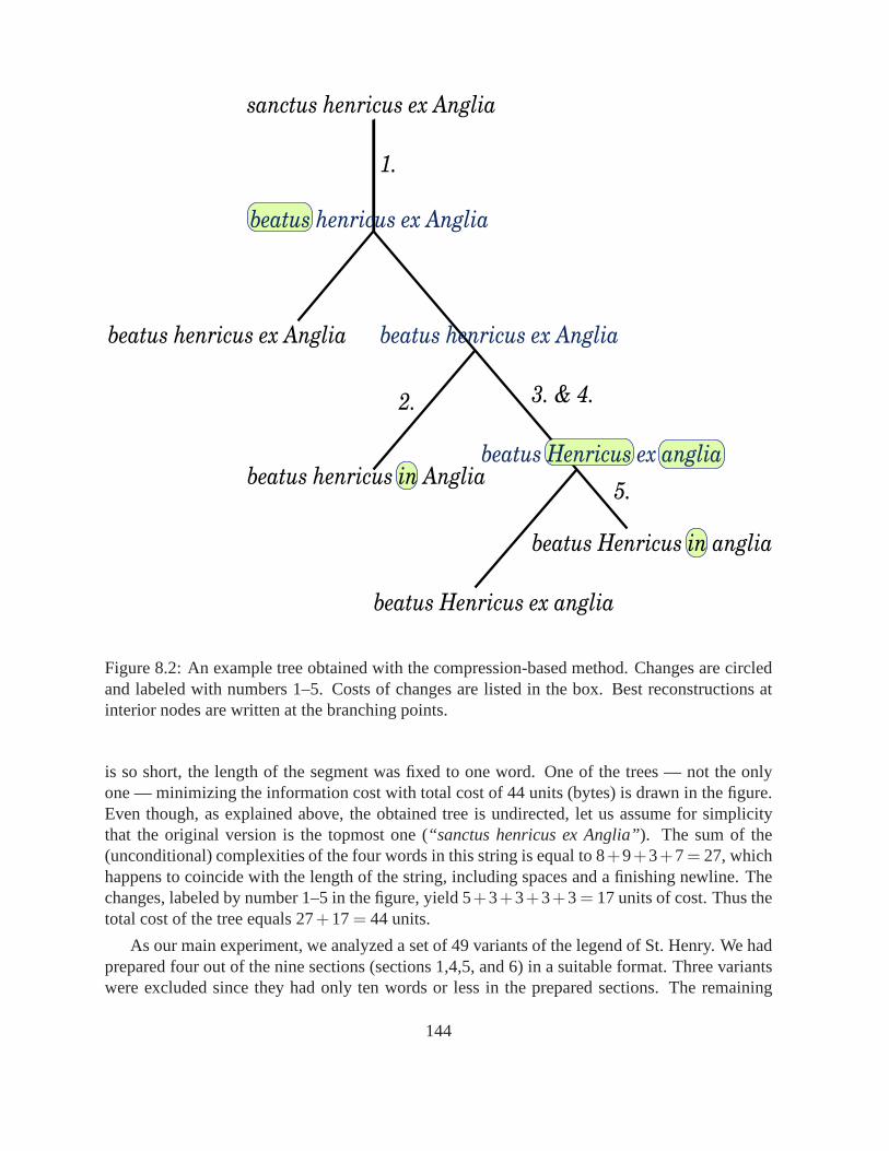
3. & 4.
1.
5.
2.
sanctus henricus ex Anglia
beatus henricus ex Anglia
beatus henricus in Anglia
beatus Henricus ex anglia
beatus Henricus in anglia
beatus henricus ex Anglia
beatus henricus ex Anglia
beatus Henricus ex anglia
Figure 8.2: An example tree obtained with the compression-based method. Changes are circledand labeled with numbers 1–5. Costs of changes are listed in the box. Best reconstructions atinterior nodes are written at the branching points.
is so short, the length of the segment was fixed to one word. Oneof the trees — not the onlyone — minimizing the information cost with total cost of 44 units (bytes) is drawn in the figure.Even though, as explained above, the obtained tree is undirected, let us assume for simplicitythat the original version is the topmost one (“sanctus henricus ex Anglia”). The sum of the(unconditional) complexities of the four words in this string is equal to 8+9+3+7= 27, whichhappens to coincide with the length of the string, includingspaces and a finishing newline. Thechanges, labeled by number 1–5 in the figure, yield 5+3+3+3+3= 17 units of cost. Thus thetotal cost of the tree equals 27+17= 44 units.
As our main experiment, we analyzed a set of 49 variants of thelegend of St. Henry. We hadprepared four out of the nine sections (sections 1,4,5, and 6) in a suitable format. Three variantswere excluded since they had only ten words or less in the prepared sections. The remaining
144
variants contained 33–379 words each. Table8.5on page150lists the estimated time or writingand place of origin, as well as the number of words in the used sections for each manuscript.The best (wrt. the information cost) tree found is shown in Fig. 8.3. By comparing the tree withearlier results [47], it can be seen that many groups of variants have been successfully placednext to each other. For instance, groups of Finnish variantsappearing in the tree that are believedto be related are Ho–I–K–T and R–S. Among the printed versions the pairs BA–BS and BLu–BLare correctly identified and also grouped close the each other5. Other pairs of variants appearingin the tree that are believed to be directly related are Li–Q (that are also correctly associatedwith BA–BS and BL–BLu), JG–B, Dr–M, NR2–JB, LT–E, AJ–D, and Bc–MN–Y. In addition,the subtree including the nine nodes between (and including) BU and Dr is rather well supportedby traditional methods. All in all, the tree corresponds very well with relationships discoveredwith more traditional methods. This is quite remarkable taking into account that in the currentexperiments we have only used four out of the nine sections ofthe legend.
In order to quantify confidence in the obtained trees we used on top of our method, block-wisebootstrap [66] and a consensus tree program in the phylogeny inference package PHYLIP [41],Section9. One hundred bootstrap samples were generated by sampling (with replacement)nsegments out of then segments that make each manuscript. The compression-basedmethoddescribed in this work was run on each bootstrap sample — thistook about a week of computa-tion — and the resulting 100 trees were analyzed with theconsense program in PHYLIP usingdefault settings (modified majority rule). The resulting consensus tree is shown in Fig.8.4.
It should be noted that the central node with nine neighbors does not corresponds to a singlemanuscript with nine descendants, but rather, that the relationships between the nine subtrees isunidentified. Because the interpretation of the consensus tree is less direct than the interpretationof the tree in Fig.8.3 as the family tree of the variants, it is perhaps best to use the consensustree to quantify the confidence in different parts of the treein Fig. 8.3. For instance, it can beseen that the pairs BL–BLu, AJ–D, Li–Q, NR2–JB, O–P, L–G, JG–B, and R–S are well sup-ported. More interestingly, The group Ho–I–K–T–A is organized in a different order in Fig.8.3and the consensus tree. This group also illustrates one of the problems in the consensus treemethod. Namely the confidence in contiguous groups that are in the middle of the tree tends tobe artificially low since the group does not make up a subtree,in this case only 3/100 (Fig.8.4).
The following potential problems and sources of bias in the resulting stemmata are roughlyin decreasing order of severity:
1. The gzip algorithm does not even attempt to fully reflect the process of imperfectly copyingmanuscripts. It remains to be studied how sensible thegzip information cost, or costs based onother compression algorithms, are in stemmatic analysis.
2. Trees are not flexible enough to represent all realistic scenarios. More than one original manuscriptmay have been used when creating a new one — a phenomenon termed contamination(or hori-zontal transfer in genomics). Point5 below may provide a solution but for non-tree structures thedynamic programming approach does not work and serious computational problems may arise.
5The printed versions are especially suspect to contamination since it is likely that more than one manuscriptwas used when composing a printed version.
145

sankoff-score 5900
Fg
Lu
VaeN
BSt
X
L
G
Cd
Dr
MVg
CV
BU
B JG
St
K
TA
I
Ho
F
De
Gh
Ef
H
R
U
S
BLu
BL
BS
BA
QLi
AJ
D
E
LT
CP
YBc
MN
O
P
JB
NR2
Figure 8.3: Best tree found. Most probable place of origin according to [47], see Ta-ble 8.5, indicated by color — Finland (blue): K,Ho,I,T,A,R,S,H,N,Fg; Vadstena (red):AJ,D,E,LT,MN,Y,JB,NR2,Li,F,G; Central Europe (yellow):JG,B; other (green). Some groupssupported by earlier work are circled in red.
3. Patching up interior node contents from 10–20 word segments is a restriction. This restriction couldbe removed for cost functions that are defined as a sum of individual words’ contributions. Suchcost functions may face problems in dealing with change of word order.
4. The number of copies made from a single manuscript can be other than zero and two. The imme-diate solution would be to use multifurcating trees in combination with our method, but this facesthe problem that the number of internal nodes strongly affects the minimum-information criterion.The modification hinted to at point5 may provide a solution to this problem.
5. Rather than looking for the tree structure that together with the optimal contents of the interior nodesminimizes the cost, it would be more principled from a probabilistic point of view to ‘marginalize’the interior nodes (see [42]). In this case we should also account for possible forms (words orsegments) not occurring in any of the observed variants.
146
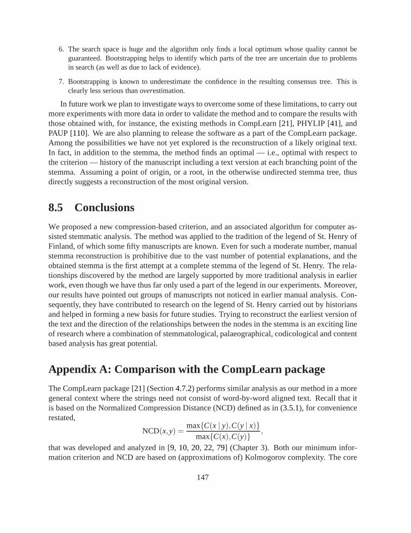
6. The search space is huge and the algorithm only finds a localoptimum whose quality cannot beguaranteed. Bootstrapping helps to identify which parts ofthe tree are uncertain due to problemsin search (as well as due to lack of evidence).
7. Bootstrapping is known to underestimate the confidence inthe resulting consensus tree. This isclearly less serious thanoverestimation.
In future work we plan to investigate ways to overcome some ofthese limitations, to carry outmore experiments with more data in order to validate the method and to compare the results withthose obtained with, for instance, the existing methods in CompLearn [21], PHYLIP [41], andPAUP [110]. We are also planning to release the software as a part of theCompLearn package.Among the possibilities we have not yet explored is the reconstruction of a likely original text.In fact, in addition to the stemma, the method finds an optimal— i.e., optimal with respect tothe criterion — history of the manuscript including a text version at each branching point of thestemma. Assuming a point of origin, or a root, in the otherwise undirected stemma tree, thusdirectly suggests a reconstruction of the most original version.
8.5 Conclusions
We proposed a new compression-based criterion, and an associated algorithm for computer as-sisted stemmatic analysis. The method was applied to the tradition of the legend of St. Henry ofFinland, of which some fifty manuscripts are known. Even for such a moderate number, manualstemma reconstruction is prohibitive due to the vast numberof potential explanations, and theobtained stemma is the first attempt at a complete stemma of the legend of St. Henry. The rela-tionships discovered by the method are largely supported bymore traditional analysis in earlierwork, even though we have thus far only used a part of the legend in our experiments. Moreover,our results have pointed out groups of manuscripts not noticed in earlier manual analysis. Con-sequently, they have contributed to research on the legend of St. Henry carried out by historiansand helped in forming a new basis for future studies. Trying to reconstruct the earliest version ofthe text and the direction of the relationships between the nodes in the stemma is an exciting lineof research where a combination of stemmatological, palaeographical, codicological and contentbased analysis has great potential.
Appendix A: Comparison with the CompLearn package
The CompLearn package [21] (Section4.7.2) performs similar analysis as our method in a moregeneral context where the strings need not consist of word-by-word aligned text. Recall that itis based on the Normalized Compression Distance (NCD) defined as in (3.5.1), for conveniencerestated,
NCD(x,y) =maxC(x | y),C(y | x)
maxC(x),C(y) ,
that was developed and analyzed in [9, 10, 20, 22, 79] (Chapter 3). Both our minimum infor-mation criterion and NCD are based on (approximations of) Kolmogorov complexity. The core
147
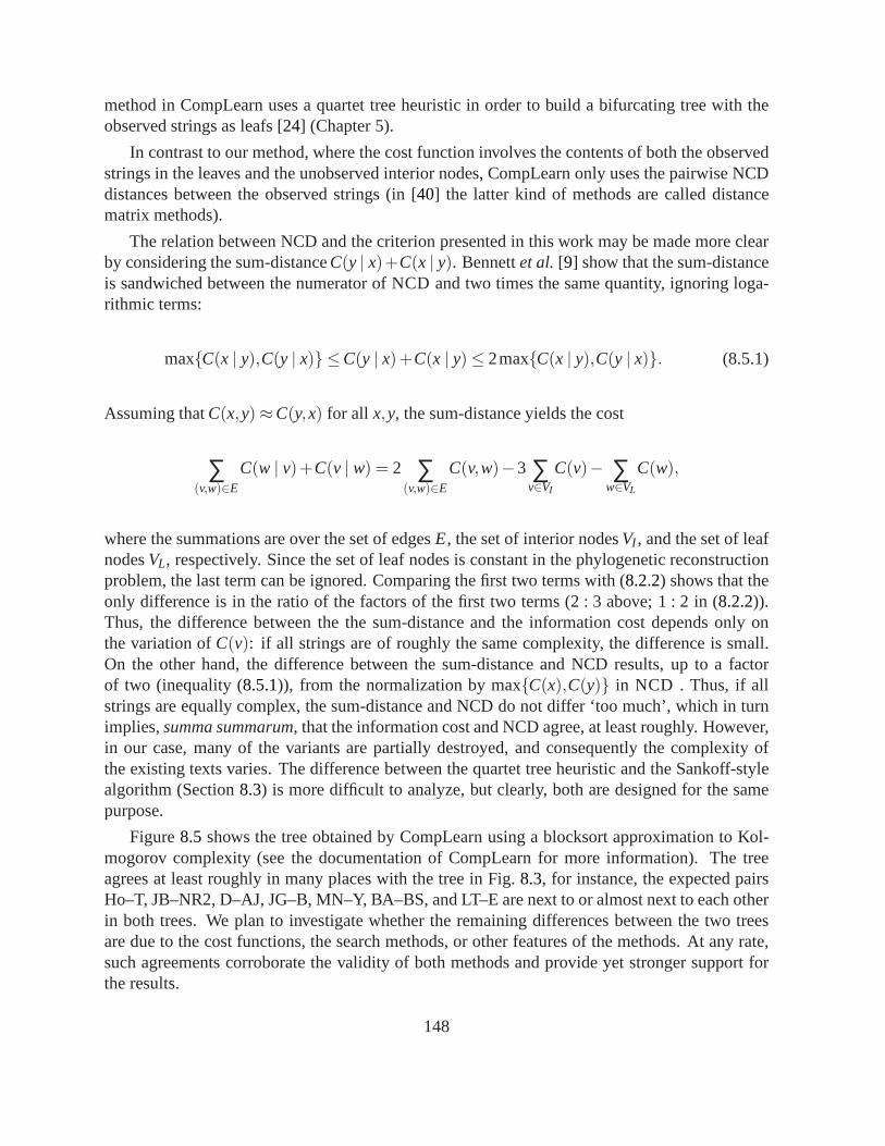
method in CompLearn uses a quartet tree heuristic in order tobuild a bifurcating tree with theobserved strings as leafs [24] (Chapter 5).
In contrast to our method, where the cost function involves the contents of both the observedstrings in the leaves and the unobserved interior nodes, CompLearn only uses the pairwise NCDdistances between the observed strings (in [40] the latter kind of methods are called distancematrix methods).
The relation between NCD and the criterion presented in thiswork may be made more clearby considering the sum-distanceC(y | x)+C(x | y). Bennettet al. [9] show that the sum-distanceis sandwiched between the numerator of NCD and two times the same quantity, ignoring loga-rithmic terms:
maxC(x | y),C(y | x) ≤C(y | x)+C(x | y)≤ 2maxC(x | y),C(y | x). (8.5.1)
Assuming thatC(x,y)≈C(y,x) for all x,y, the sum-distance yields the cost
∑(v,w)∈E
C(w | v)+C(v | w) = 2 ∑(v,w)∈E
C(v,w)−3 ∑v∈VI
C(v)− ∑w∈VL
C(w),
where the summations are over the set of edgesE, the set of interior nodesVI , and the set of leafnodesVL, respectively. Since the set of leaf nodes is constant in thephylogenetic reconstructionproblem, the last term can be ignored. Comparing the first twoterms with (8.2.2) shows that theonly difference is in the ratio of the factors of the first two terms (2 : 3 above; 1 : 2 in (8.2.2)).Thus, the difference between the the sum-distance and the information cost depends only onthe variation ofC(v): if all strings are of roughly the same complexity, the difference is small.On the other hand, the difference between the sum-distance and NCD results, up to a factorof two (inequality (8.5.1)), from the normalization by maxC(x),C(y) in NCD . Thus, if allstrings are equally complex, the sum-distance and NCD do notdiffer ‘too much’, which in turnimplies,summa summarum, that the information cost and NCD agree, at least roughly. However,in our case, many of the variants are partially destroyed, and consequently the complexity ofthe existing texts varies. The difference between the quartet tree heuristic and the Sankoff-stylealgorithm (Section8.3) is more difficult to analyze, but clearly, both are designedfor the samepurpose.
Figure8.5 shows the tree obtained by CompLearn using a blocksort approximation to Kol-mogorov complexity (see the documentation of CompLearn formore information). The treeagrees at least roughly in many places with the tree in Fig.8.3, for instance, the expected pairsHo–T, JB–NR2, D–AJ, JG–B, MN–Y, BA–BS, and LT–E are next to oralmost next to each otherin both trees. We plan to investigate whether the remaining differences between the two treesare due to the cost functions, the search methods, or other features of the methods. At any rate,such agreements corroborate the validity of both methods and provide yet stronger support forthe results.
148

It should be realized that the structure of the output trees in the two cases are different. Thisis due to differences in constraints and assumptions as wellas explicit algorithmic differences asalready noted. Thus, not too many conclusions should be drawn from this rough comparison.
149
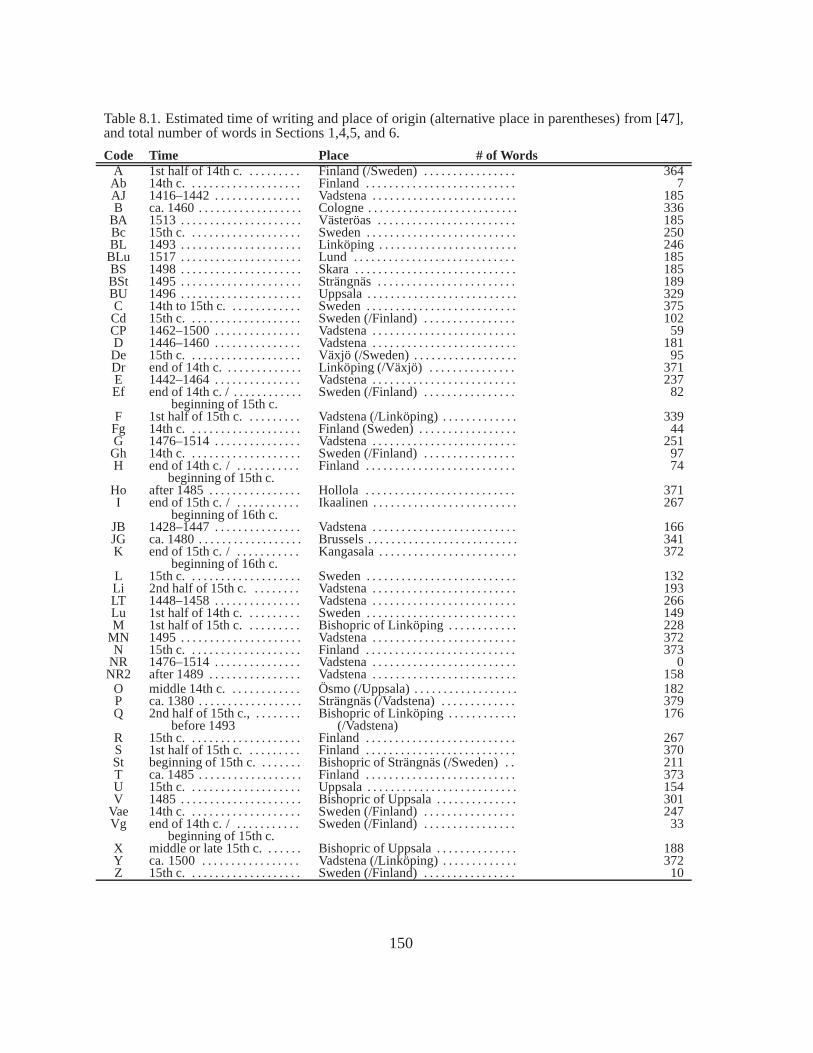
Table 8.1. Estimated time of writing and place of origin (alternative place in parentheses) from [47],and total number of words in Sections 1,4,5, and 6.
Code Time Place # of WordsA 1st half of 14th c. . . . . . . . . . Finland (/Sweden) . . . . . . . . . .. . . . . . 364Ab 14th c. . . . . . . . . . . . . . . . . . . . Finland . . . . . . . . . . . . . . . . .. . . . . . . . . 7AJ 1416–1442 . . . . . . . . . . . . . . . Vadstena . . . . . . . . . . . . . . . . .. . . . . . . . 185B ca. 1460 . . . . . . . . . . . . . . . . . . Cologne . . . . . . . . . . . . . . . . . .. . . . . . . . 336
BA 1513 . . . . . . . . . . . . . . . . . . . . . Västeröas . . . . . . . . . . . . . . .. . . . . . . . . 185Bc 15th c. . . . . . . . . . . . . . . . . . . . Sweden . . . . . . . . . . . . . . . . . .. . . . . . . . 250BL 1493 . . . . . . . . . . . . . . . . . . . . . Linköping . . . . . . . . . . . . . . .. . . . . . . . . 246BLu 1517 . . . . . . . . . . . . . . . . . . . . . Lund . . . . . . . . . . . . . . . . . . .. . . . . . . . . 185BS 1498 . . . . . . . . . . . . . . . . . . . . . Skara . . . . . . . . . . . . . . . . . . .. . . . . . . . . 185BSt 1495 . . . . . . . . . . . . . . . . . . . . . Strängnäs . . . . . . . . . . . . . .. . . . . . . . . . 189BU 1496 . . . . . . . . . . . . . . . . . . . . . Uppsala . . . . . . . . . . . . . . . . .. . . . . . . . . 329C 14th to 15th c. . . . . . . . . . . . . Sweden . . . . . . . . . . . . . . . . . . . .. . . . . . 375Cd 15th c. . . . . . . . . . . . . . . . . . . . Sweden (/Finland) . . . . . . . .. . . . . . . . 102CP 1462–1500 . . . . . . . . . . . . . . . Vadstena . . . . . . . . . . . . . . . . .. . . . . . . . 59D 1446–1460 . . . . . . . . . . . . . . . Vadstena . . . . . . . . . . . . . . . . . .. . . . . . . 181De 15th c. . . . . . . . . . . . . . . . . . . . Växjö (/Sweden) . . . . . . . . . .. . . . . . . . 95Dr end of 14th c. . . . . . . . . . . . . . Linköping (/Växjö) . . . . . . . .. . . . . . . 371E 1442–1464 . . . . . . . . . . . . . . . Vadstena . . . . . . . . . . . . . . . . . .. . . . . . . 237Ef end of 14th c. / . . . . . . . . . . . . Sweden (/Finland) . . . . . . . . .. . . . . . . 82
beginning of 15th c.F 1st half of 15th c. . . . . . . . . . Vadstena (/Linköping) . . . . . .. . . . . . . 339Fg 14th c. . . . . . . . . . . . . . . . . . . . Finland (Sweden) . . . . . . . . .. . . . . . . . 44G 1476–1514 . . . . . . . . . . . . . . . Vadstena . . . . . . . . . . . . . . . . . .. . . . . . . 251Gh 14th c. . . . . . . . . . . . . . . . . . . . Sweden (/Finland) . . . . . . . .. . . . . . . . 97H end of 14th c. / . . . . . . . . . . . Finland . . . . . . . . . . . . . . . . . . . .. . . . . . 74
beginning of 15th c.Ho after 1485 . . . . . . . . . . . . . . . . Hollola . . . . . . . . . . . . . . . . .. . . . . . . . . 371I end of 15th c. / . . . . . . . . . . . Ikaalinen . . . . . . . . . . . . . . . . . .. . . . . . . 267
beginning of 16th c.JB 1428–1447 . . . . . . . . . . . . . . . Vadstena . . . . . . . . . . . . . . . . .. . . . . . . . 166JG ca. 1480 . . . . . . . . . . . . . . . . . . Brussels . . . . . . . . . . . . . . . .. . . . . . . . . . 341K end of 15th c. / . . . . . . . . . . . Kangasala . . . . . . . . . . . . . . . . . .. . . . . . 372
beginning of 16th c.L 15th c. . . . . . . . . . . . . . . . . . . . Sweden . . . . . . . . . . . . . . . . . . .. . . . . . . 132Li 2nd half of 15th c. . . . . . . . . Vadstena . . . . . . . . . . . . . . . . . .. . . . . . . 193LT 1448–1458 . . . . . . . . . . . . . . . Vadstena . . . . . . . . . . . . . . . . .. . . . . . . . 266Lu 1st half of 14th c. . . . . . . . . . Sweden . . . . . . . . . . . . . . . . . . .. . . . . . . 149M 1st half of 15th c. . . . . . . . . . Bishopric of Linköping . . . . . .. . . . . . 228
MN 1495 . . . . . . . . . . . . . . . . . . . . . Vadstena . . . . . . . . . . . . . . . .. . . . . . . . . 372N 15th c. . . . . . . . . . . . . . . . . . . . Finland . . . . . . . . . . . . . . . . . .. . . . . . . . 373
NR 1476–1514 . . . . . . . . . . . . . . . Vadstena . . . . . . . . . . . . . . . . .. . . . . . . . 0NR2 after 1489 . . . . . . . . . . . . . . . . Vadstena . . . . . . . . . . . . . . .. . . . . . . . . . 158
O middle 14th c. . . . . . . . . . . . . Ösmo (/Uppsala) . . . . . . . . . . . .. . . . . . 182P ca. 1380 . . . . . . . . . . . . . . . . . . Strängnäs (/Vadstena) . . . . .. . . . . . . . 379Q 2nd half of 15th c., . . . . . . . . Bishopric of Linköping . . . . . .. . . . . . 176
before 1493 (/Vadstena)R 15th c. . . . . . . . . . . . . . . . . . . . Finland . . . . . . . . . . . . . . . . . .. . . . . . . . 267S 1st half of 15th c. . . . . . . . . . Finland . . . . . . . . . . . . . . . . . . .. . . . . . . 370St beginning of 15th c. . . . . . . . Bishopric of Strängnäs (/Sweden) . . 211T ca. 1485 . . . . . . . . . . . . . . . . . . Finland . . . . . . . . . . . . . . . . . .. . . . . . . . 373U 15th c. . . . . . . . . . . . . . . . . . . . Uppsala . . . . . . . . . . . . . . . . . .. . . . . . . . 154V 1485 . . . . . . . . . . . . . . . . . . . . . Bishopric of Uppsala . . . . . . .. . . . . . . 301
Vae 14th c. . . . . . . . . . . . . . . . . . . . Sweden (/Finland) . . . . . . .. . . . . . . . . 247Vg end of 14th c. / . . . . . . . . . . . Sweden (/Finland) . . . . . . . . . .. . . . . . 33
beginning of 15th c.X middle or late 15th c. . . . . . . Bishopric of Uppsala . . . . . . . .. . . . . . 188Y ca. 1500 . . . . . . . . . . . . . . . . . Vadstena (/Linköping) . . . . . .. . . . . . . 372Z 15th c. . . . . . . . . . . . . . . . . . . . Sweden (/Finland) . . . . . . . . .. . . . . . . 10
150
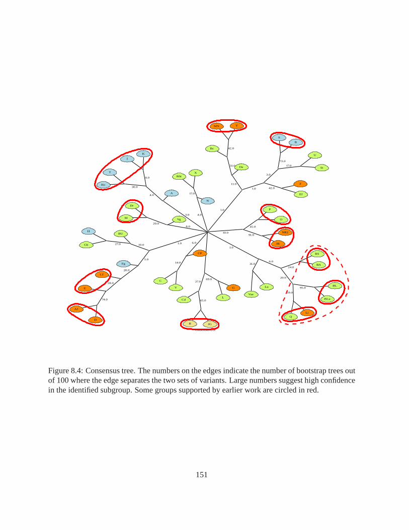
consensus-tree
69.0
G
L
4.0
27.0
1.0
1.0
1.0
3.0 4.0
8.0
10.0
6.0
6.031.0
24.0
20.0
BS
BA
95.0
59.0
BL
BLu
Q
Li
Lu
Vae
1.0
11.0
3.0
42.0
17.0
72.0
St
U
S
R
Ef
F
31.0 De
42.0Bc
MN Y
5.0
10.0
Fg
20.0
28.0
LT
74.0
E
AJ
D
27.0
BU
Gh
H
A4.0
8.0
30.0
K
I
Ho
T
N
17.0
BStX
Vg
29.0
Dr
M
45.0
91.0
O
P
NR2
JB
CP
14.0
C
V
65.0Cd
JGB
Figure 8.4: Consensus tree. The numbers on the edges indicate the number of bootstrap trees outof 100 where the edge separates the two sets of variants. Large numbers suggest high confidencein the identified subgroup. Some groups supported by earlierwork are circled in red.
151
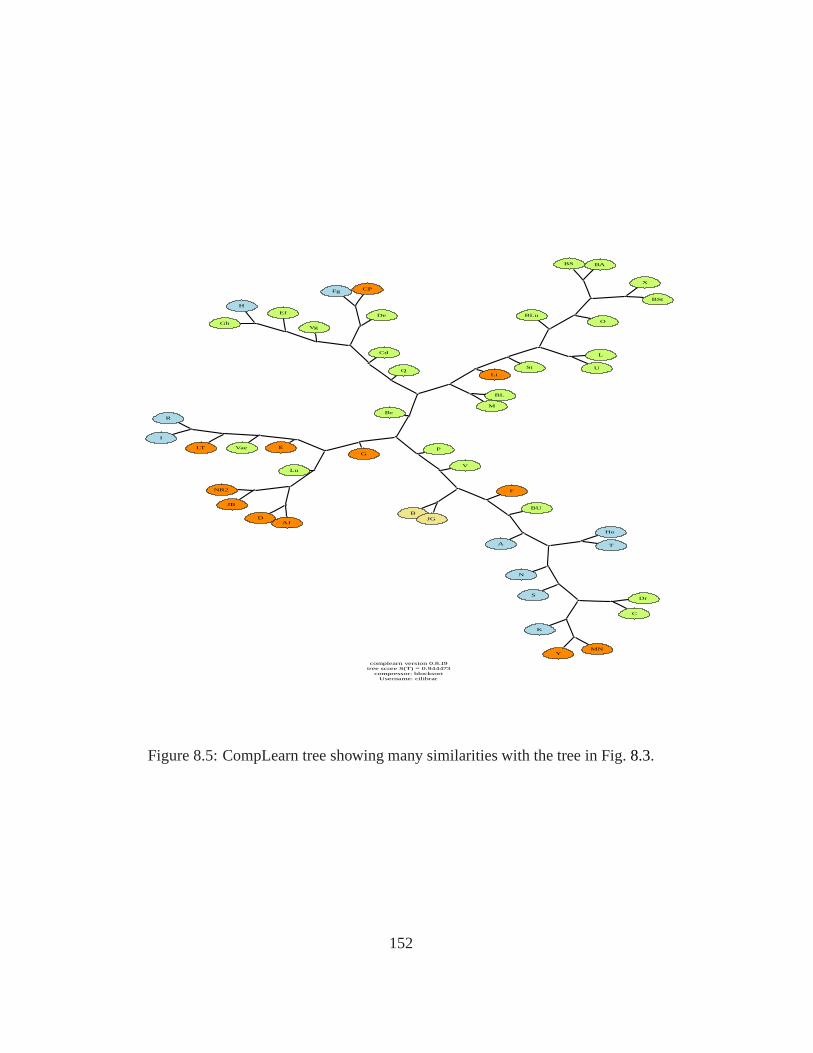
complearn version 0.8.19tree score S(T) = 0.944473
compressor: blocksortUsername: cilibrar
X
BSt
BS BA
OBLu
St
LiQ
Cd
Vg
Ef
Gh
H
De
CPFg
Bc
P
V
F
BU
A
Ho
T
N
S
K
YMN
Dr
C
BJG
G
Lu
DAJ
NR2
JB
EVaeLT
I
R
BL
M
U
L
Figure 8.5: CompLearn tree showing many similarities with the tree in Fig.8.3.
152
Chapter 9
Comparison of CompLearn with PHYLIP
In tree reconstruction systems like PHYLIP, trees are constructed in a greedy fashion using a ran-domly permuted ordering. Many different permutations are sampled and tree-splits are classifiedaccording to how consistently they come up with a score from 0to 100 indicating a percentageagreement. This results in a so-called “consensus tree”. While this method is far quicker thanours for large trees, it is probably in certain situations more error prone. It does not directlyaddress the whole tree as one structured object but instead says something about the most likelypaths where trees are iteratively increased one step at a time. Another difficulty of this approachis that sometimes bootstrap values are just too low, less than 50 for all splits, in which casePHYLIP’s answer is considered too suspicious to use. In our technique this is rarely the case be-cause we start with a random tree and make a monotonic sequence of nondeterministic steps toimprove it. Our algorithm will always produce something better than random in practice and typ-ically produces something reasonably good for natural data. Another problem with PHYLIP andthe like is that there are many parameters and adjustments that must be made in order to properlycalculate distances in the matrix creation phase; further,there are many choices of parameters inthe tree-building phase so it takes more effort to use.
The most difficult part is a multiple-alignment phase that typically involves a biology expert.For comparison, The kitsch program in PHYLIP was run with theH5N1 distance matrix to buildthe tree. The kitsch program is generally considered the most accurate in the PHYLIP suite.Using a random seed value of 1 and generating 100 different random orderings for 100 differenttrees of 100 nodes yields the consensus tree of Figure9.1. A casual observation and comparisonwith Figure4.10 indicates that this tree is largely similar but not identical to the CompLearnoutput. This is attributed to the fact that theS(T) score is quite high suggesting that the inputdata distance matrix has very good projection to a binary tree without substantial distortion andthus serves as a relatively “easy” case of the difficult problem domain. CompLearn shows amore clear advantage in the next experiment involving 102 Nobel prize winning writers. Here,NGD is used to generate the distance matrix in a quantitativeway similar to the newly popularapproaches such as Moretti’s [84]:
Theories are nets, and we should learn to evaluate them for the empirical data theyallow us to process and understand: for how they concretely change the way we
153
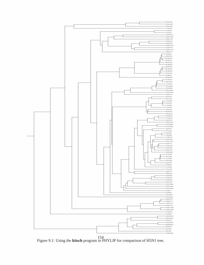
ChHebei108
DuAnyangAV
DuShandong
swineShand
swineFujib
swineFujia
ChHKYU822.
ChHKYU5620
CkHK31.402
GoHK3014.8
DuHK2986.1
PhHKFY1550
ChHKNT873.
ChHKFY1500
ChHebei718
GuQi305m
BGQi6105m
BGQi5905m
BGQi505m
BGQi1205m
BGQi6805m
BGQi6705m
BGQi6205m
BGQi6505m
BGQi7505m
GreatBlack
BGQi6005m
crowKyoto5
ChKyoto304
crowOsaka1
ChYamaguch
ChOita804m
DuKoreaESD
ChGD17404m
ChHebei326
grebeNovos
DuNovosibi
CyAsAst08-
CyAsAst07-
CyAsAst05-
CyAsAst06-
whooperswa
BGMo105m
ChKurgan30
ChThNontab
ChThKancha
quailThNak
ThNK16505m
ChViC5804m
CkViC5704m
tigerThCU-
ChAyutthay
tigerSupha
leopardSup
catThKU-02
Th2SP-3304
Th1KAN-104
birdTh3.10
CkTh9.104m
QaTh5704m
ChNakorn-P
Th5KK-4940
CkVi3804m
CkVi3504m
CkVi3604m
CkVi3704m
quailVi360
Vi306204m
Vi119404m
CkVi3304m
egretHK757
ChHubei327
CkInPA03m
CkInBL03m
DkInMS04m
DuChinaE31
ChGD17804m
ChGD19104m
DuGD17304m
peregrinef
ChJilin904
ChHubei489
DuYokohama
EnHK437-89
EnHK437-10
EnHK437-49
EnHK437-69
GoHKww2800
GoHKww2600
GoGD196m
GoGD397m
ChHK78697m
ChHK72897m
HK54297m
GoHKw35597
DuHKp4697m
HK48297m
HK53897m
HK9798m
ChHK25897m
Figure 9.1: Using thekitsch program in PHYLIP for comparison of H5N1 tree.154

work, rather than as ends in themselves. Theories are nets; and there are so manyinteresting creatures that await to be caught, if only we try. – Moretti
Here, the maximal score is not as high as the H5N1 tree. The PHYLIP package does not copeas well with the ambiguities and seems to produce a much quicker yet obviously lower qualitytree as shown below. The clustering of American and British writers is more scattered. This runused 100 jumbles (random permutations) to form the consensus. This strategy of simple randompermutation based sampling serves to increase the effective power of PHYLIP considerably, butdoes not work very well to get high-accuracy plots of high-inconsistency data which often occurin practice.
155
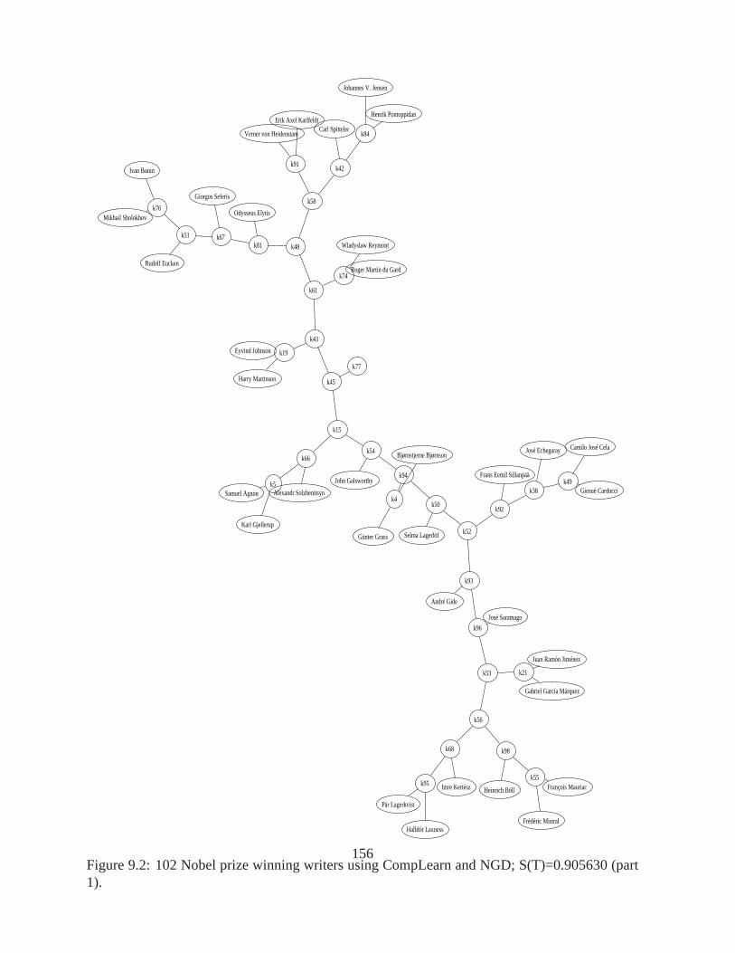
k77
k45
k43
k15
k61
k19
k74
k48 Wladyslaw Reymont
Roger Martin du Gard
k81
k58
Odysseus Elytis
k67
Giorgos Seferis
k51
Rudolf Eucken
k76Mikhail Sholokhov
Ivan Bunink91
k42
Erik Axel Karlfeldt
Verner von HeidenstamCarl Spitteler
k84
Henrik Pontoppidan
Johannes V. Jensen
Harry Martinson
Eyvind Johnson
k66k54
Alexandr Solzhenitsynk5
Karl Gjellerup
Samuel Agnon
John Galsworthyk94
k50k4
Selma Lagerlöf k52
k93
k92
André Gide
k96
José Saramago
k53
k56
k21
k98k68
Heinrich Böll
k55François Mauriac
Frédéric Mistral
Imre Kertészk95
Pär Lagerkvist
Halldór Laxness
Juan Ramón Jiménez
Gabriel García Márquez
Frans Eemil Sillanpää
k38
José Echegaray
k49
Camilo José Cela
Giosuè Carducci
Günter Grass
Bjørnstjerne Bjørnson
Figure 9.2: 102 Nobel prize winning writers using CompLearnand NGD; S(T)=0.905630 (part1).
156
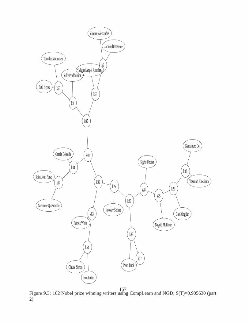
k77
k33
Pearl Buck
k39
k28k26
Sigrid Undset
k75
Naguib Mahfouz
k29
Gao Xingjian
k30
Kenzaburo Oe
Yasunari Kawabata
Jaroslav Seifert
k36
k83
k40
Patrick White
k64
Claude Simon
Ivo Andric
k85
k44
k65
k3
Miguel Angel Asturiask2
Vicente Aleixandre
Jacinto Benavente
Sully Prudhomme
k63Paul Heyse
Theodor Mommsen
Grazia Deledda
k97
Salvatore Quasimodo
Saint-John Perse
Figure 9.3: 102 Nobel prize winning writers using CompLearnand NGD; S(T)=0.905630 (part2).
157

Figure 9.4: 102 Nobel prize winning writers using CompLearnand NGD; S(T)=0.905630 (part3).
158

ShawBernar
RussellBer
HemingwayE
MiloszCzes
Szymborska
HeaneySeam
NaipaulVSm
LewisSincl
BellowSaul
SoyinkaWol
GordimerNa
WalcottDer
KawabataYa
OeKenzabur
AsturiasAn
SimonClaud
MartinsonH
JohnsonEyv
GjellerupK
Galsworthy
AgnonSamue
Pontoppida
SeferisGio
EuckenRudo
Heidenstam
KarlfeldtA
ElytisOdys
GardduMart
BuninIvanm
SpittelerC
JensenVJoh
ReymontWla
SholokhovM
SeifertJar
PrudhommeS
AndricIvom
MommsenThe
XingjianGa
PerseSaint
BenaventeJ
Aleixandre
DeleddaGra
WhitePatri
BrodskyJos
HamsunKnut
UndsetSigr
MahfouzNag
SachsNelly
PasternakB
BuckPearlm
QuasimodoS
MontaleEug
BergsonHen
Sienkiewic
SingerBash
HeysePaulm
Maeterlinc
Pirandello
RollandRom
MistralGab
PazOctavio
Solzhenits
TagoreRabi
CoetzeeJMm
FranceAnat
ONeillEuge
CanettiEli
GoldingWil
HauptmannG
CamusAlber
SartreJean
BeckettSam
MannThomas
HesseHerma
FaulknerWi
SteinbeckJ
MorrisonTo
YeatsButle
FoDariom
KiplingRud
NerudaPabl
JelinekElf
PinterHaro
EchegarayJ
CelaJosØCa
SillanpääE
CarducciGi
GideAndrØm
SaramagoJo
LagerlöfSe
MistralFrØ
Lagerkvist
LaxnessHal
BjłrnsonBj
GrassGünte
BöllHeinri
KertØszImr
MauriacFra
EliotTSm
MÆrquezGar
JimØnezRam
ChurchillW
Figure 9.5: 102 Nobel prize winning writers using the PHYLIPkitsch.159

Chapter 10
CompLearn Documentation
This chapter presents an overview of the CompLearn system. It provides a functional descriptionfrom a high level followed by a detailed manual for basic installation and use. The material inthis chapter will be useful for those wanting to run their ownexperiments using the CompLearndata mining system.
We start with a current snapshot of some important documentation for the CompLearn soft-ware system is presented. It is the core software behind almost all experiments mentioned inthis thesis and represents a first general purpose open source data compression based learningsystem. The following documentation is literally copied from the online website and the readeris referred tohttp://complearn.org/ for more info.1
What is CompLearn?CompLearn is a suite of simple-to-use utilities that you canuse to apply compression tech-
niques to the process of discovering and learning patterns.The compression-based approach used is powerful because itcan mine patterns in completely
different domains. It can classify musical styles of piecesof music and identify unknown com-posers. It can identify the language of bodies of text. It candiscover the relationships betweenspecies of life and even the origin of new unknown viruses such as SARS. Other uncharted areasare up to you to explore.
In fact, this method is so general that it requires no background knowledge about any partic-ular classification. There are no domain-specific parameters to set and only a handful of generalsettings. Just feed and run.
Installation InstallationCompLearn was packaged usingAutoconf. Installation steps:
$ ./configure$ make$ make install
1 It should be mentioned that in recent time the CompLearn system has had an improvement made which is notexplained in the previously published literature. It concerns the dotted lines around the edge nodes on trees withnumerical scores in the middle, see Chapter7, Section7.5.3.
161
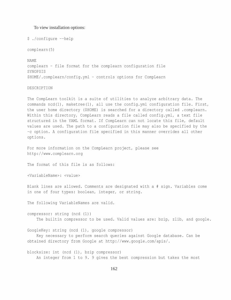
To view installation options:
$ ./configure --help
complearn(5)
NAMEcomplearn - file format for the complearn configuration fileSYNOPSIS$HOME/.complearn/config.yml - controls options for CompLearn
DESCRIPTION
The CompLearn toolkit is a suite of utilities to analyze arbitrary data. Thecommands ncd(1), maketree(1), all use the config.yml configuration file. First,the user home directory ($HOME) is searched for a directory called .complearn.Within this directory, CompLearn reads a file called config.yml, a text filestructured in the YAML format. If CompLearn can not locate this file, defaultvalues are used. The path to a configuration file may also be specified by the-c option. A configuration file specified in this manner overrides all otheroptions.
For more information on the CompLearn project, please seehttp://www.complearn.org
The format of this file is as follows:
<VariableName>: <value>
Blank lines are allowed. Comments are designated with a # sign. Variables comein one of four types: boolean, integer, or string.
The following VariableNames are valid.
compressor: string (ncd (1))The builtin compressor to be used. Valid values are: bzip, zlib, and google.
GoogleKey: string (ncd (1), google compressor)Key necessary to perform search queries against Google database. Can be
obtained directory from Google at http://www.google.com/apis/.
blocksize: int (ncd (1), bzip compressor)An integer from 1 to 9. 9 gives the best compression but takes the most
162
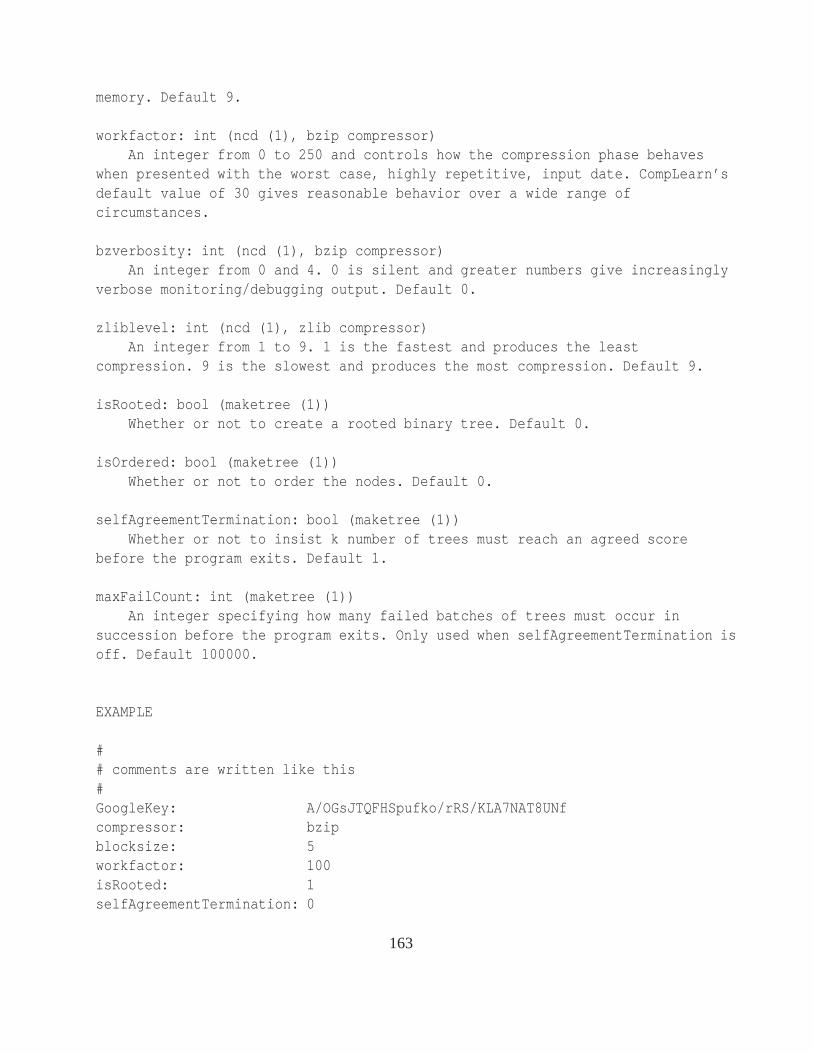
memory. Default 9.
workfactor: int (ncd (1), bzip compressor)An integer from 0 to 250 and controls how the compression phase behaves
when presented with the worst case, highly repetitive, input date. CompLearn’sdefault value of 30 gives reasonable behavior over a wide range ofcircumstances.
bzverbosity: int (ncd (1), bzip compressor)An integer from 0 and 4. 0 is silent and greater numbers give increasingly
verbose monitoring/debugging output. Default 0.
zliblevel: int (ncd (1), zlib compressor)An integer from 1 to 9. 1 is the fastest and produces the least
compression. 9 is the slowest and produces the most compression. Default 9.
isRooted: bool (maketree (1))Whether or not to create a rooted binary tree. Default 0.
isOrdered: bool (maketree (1))Whether or not to order the nodes. Default 0.
selfAgreementTermination: bool (maketree (1))Whether or not to insist k number of trees must reach an agreed score
before the program exits. Default 1.
maxFailCount: int (maketree (1))An integer specifying how many failed batches of trees must occur in
succession before the program exits. Only used when selfAgreementTermination isoff. Default 100000.
EXAMPLE
## comments are written like this#GoogleKey: A/OGsJTQFHSpufko/rRS/KLA7NAT8UNfcompressor: bzipblocksize: 5workfactor: 100isRooted: 1selfAgreementTermination: 0
163

maxFailCount: 50000# etc
FILES$HOME/.complearn/config.yml
configuration file, overrides system default
164
Usage: ncd [OPTION] ... [FILE | STRING | DIR ] [FILE | STRING | DIR]
ENUMERATION MODES:-f, --file-mode=FILE file; default mode-l, --literal-mode=STRING string literal-p, --plainlist-mode=FILE list of file names by linebreaks-t, --termlist-mode=FILE list of string literals separated by linebreaks-d, --directory-mode=DIR directory of files-w, --windowed-mode=FILE,firstpos,stepsize,width,lastpos
file be separated into windows
NCD OPTIONS:-C, --compressor=STRING use builtin compressor-L, --list list of available builtin compressors-g, --google use Google compression (NGD)-D, --delcache clear the Google cache-o, --outfile=distmatname set the default distance matrix output name-r, --realcomp=pathname use real compressor, passing in pathname of
compressor
OPTIONS:-c, --config-file=FILE in YAML format-S, --size compressed size 1 FILE, STRING or DIR-x, --exp print out 2^val instead of val-B, --binary enable binary output mode-P, --svd-project output a singular value decomposition matrix-s, --suppress suppress ASCII output-b, --both enable both binary and text output mode-H, --html output in HTML format-P, --svd-project activate SVD projection mode-r, --suppressdetails do not print details to dot file-V, --version-v, --verbose-h, --help
165
Usage: maketree [OPTION] ... FILE
MAKETREE OPTIONS:-o, --outfile=treename set the default tree output name-R, --rooted create rooted tree-O, --ordered create ordered tree-T, --text-input format of distance matrix is text-F disable self agreement termination and enable
max fail count
OPTIONS:-c, --config-file=FILE in YAML format-S, --size compressed size 1 FILE, STRING or DIR-x, --exp print out 2^val instead of val-B, --binary enable binary output mode-P, --svd-project output a singular value decomposition matrix-s, --suppress suppress ASCII output-b, --both enable both binary and text output mode-H, --html output in HTML format-P, --svd-project activate SVD projection mode-r, --suppressdetails do not print details to dot file-V, --version-v, --verbose-h, --help
166
CompLearn FAQ
1. What is CompLearn?
CompLearn is a software system built to support compression-based learning in awide variety of applications. It provides this support in the form of a librarywritten in highly portable ANSI C that runs in most modern computerenvironments with minimal confusion. It also supplies a small suite of simple,composable command-line utilities as simple applications that use this library.Together with other commonly used machine-learning tools such as LIBSVM andGraphViz, CompLearn forms an attractive offering in machine-learning frameworksand toolkits. It is designed to be extensible in a variety of ways includingmodular dynamic-linking plugins (like those used in the Apache webserver) and alanguage-neutral SOAP interface to supply instant access to core functionalityin every major language.
2. Why did the version numbers skip so far between 0.6.4 and 0.8.12?
In early 2005 a major rewrite occurred. This was due to poor organization ofthe original complearn package, leading to compilation and installationdifficulties in far too many situations. This issue was addressed by using acomplete rewrite from the ground up of all functionality; earlier versions useda combination of C and Ruby to deliver tree searching. The new version deliversall core functionality, such as NCD and tree searching, in a pure C library. Ontop of this library is layered a variety of other interfaces such as SOAP and anew in-process direct-extension CompLearn Ruby binding layer. But alldependencies have been reworked and are now modularized so that Ruby and almostevery other software package is now optional and a variety of differentconfigurations will compile cleanly.
Another major enhancement in the new complearn is the addition of a Googlecompressor to calculate NGD. This has opened up whole new areas of QuantitativeSubjective Analysis (QSA) to complement our existing more classically purestatistical methods in earlier gzip-style NCD research. By querying the Googlewebserver through a SOAP layer we may convert page counts of search terms tovirtual file lengths that can be used to determine semantic relationshipsbetween terms. Please see the paper Automatic Meaning Discovery Using Googlefor more information.
3. I can’t get the Google compressor to work. When Itype ncd -L, it’s not even listed as one of the builtin compressors. What am Idoing wrong?
167

You may not have the csoap library installed, which is necessary for the Googlecompressor to work. You can check this when you run your ./configure commandduring the CompLearn installation phase. A "NO" in the CompLearn dependencytable for csoap indicates you need to install the csoap library.
You can download csoap at the following link:
http://sourceforge.net/project/showfiles.php?group_id=74977
Once csoap is installed, you will need to run the ./configure command again(for CompLearn), perhaps with a "--with-csoap" option depending on the locationof the csoap installation. For more options, you can type
./configure --help
Please see our Dependencies section for more information on CompLearn librarydependencies.
4. The Windows demo isn’t working for me? Why not?
If you have cygwin installed on your computer, it’s very likely you need toupdate it. The CompLearn Windows demo uses version 1.5.17 of the cygwin dll;any previous versions are not compatible with the demo. To update your cygwin,go to http://cygwin.com and hit the Install or Update now link.
You may also need to download and install DirectX.5. gsl and CompLearn seemed to install perfectly, but ncd can’t load the gsllibrary.
Users may get the following message if this happens:
ncd: error while loading shared libraries: libgslcblas.so.0: cannotopen shared object file: No such file or directory
If this is the case, your LD_LIBRARY_PATH environment variable may need to beset. For example, you can try the following before running the ncd command:
export LD_LIBRARY_PATH=/usr/local/lib
6. How can this demo work with only 1000 queries a day?
There are two reasons this demo is able to do as much as it does. One is thatGoogle has generously (and free of charge to me) upgraded my Google API account
168
key daily search limit. You might email them to ask yourself if you have aninteresting Google API based search application of your own. The other reasonthe demo works is because there is a cache of recent page result counts. Youcan see this cache by looking in the $HOME/.complearn directory. Sometimeslarger experiments must be run over the course of two days.
7. How come the counts returned from (any particular) Google API are differentthat the numbers I see when I enter searches by hand?
I have two possible explanations for this behavior. One is that it would beprohibitively expensive to count the exact total of all pages indexed for mostcommon search terms. Instead they use an estimation heuristic called"prefixing" whereby they just use a short sample of webpages as arepresentative set for the web and scale up as appropriate. I presume this andalso that when you do a search (either by hand or from the API) you can getconnected to any one of a number of different search servers, each with aslightly different database. In a rapidly changing large global network it isunlikely that there will be an exact match for the counts on any particularcommon term because each server must maintain its own distinct "aging snapshot"of the internet.
8. When I compile csoap, I don’t seem to be getting sharedlibraries. Or even though csoap is installed, complearn doesn’t seem to bedetecting the shared library.
Try compiling csoap from source with the following options:
--with-libxml-prefix=/usr --enable-shared --with-pic
Then try reconfiguring and recompiling complearn.
Thanks to Tsu Do Nimh for this tip.
9. Is it important to adjust or choose a compressor? How should I do it?
Yes, it is very important to choose a good compressor for your application. The"blocksort" compressor is the current default. It is a virtual compressor usinga simple blocksorting algorithm. It will give results something like frequencyanalysis, spectral analysis, and substring matching combined. It works verywell for small strings (or files) of 100 bytes or less. If you have more thanabout 100 bytes then it is probably better to use one of the other threefavorite compressors other than the default:
169
ncd -C zlib
will get you "zlib" style compression which is like gzip and is limited tofiles of up to 15K in size.
ncd -C bzip
will get you "bzip2" style compression which is like zlib but allows for filesup to about 450K in size. The best accuracy is available using the "realcompressor" shell option. For this to work you need to use a script like this:
#!/bin/bashcd /tmpcat >infile/ufs/cilibrar/bin/ppmd e infile >/dev/null </dev/null 2>/dev/nullcat infile.pmdrm infile infile.pmd
If you install that script in $HOME/bin/catppmd and don’t forget to chmod itexecutable (using chmod a+rx $HOME/bin/catppmd for instance) then you can useit with the following option to ncd:
ncd -r $HOME/bin/catppmd
10. Running ./configure gives me the following error: cannot find input file:src/complearn/aclconfig.h.in. Where can I find this file?
You will need to generate this header input file by running the autoheadercommand. autoheader is packaged with autoconf.
autoheader
11. I get the configure error: Can’t locate object method "path" via package"Request" at /usr/share/autoconf/Autom4te/C4che.pm line 69, line 111. make[1]:*** [configure] Error 1. Is there an easy way to fix this?
In the top directory of the CompLearn distribution, run the following commands:
rm -rf autom4te.cache
or
make maintainer-clean
170

171


Bibliography
[1] M.J. Alberink, L.W. Rutledge, and M.J.A. Veenstra. Clustering semantics for hypermediapresentation. Technical Report INS-E0409, CWI, 2004. ISSN1386-3681.7.5.2
[2] W. Haken Appel, K. I. and J. Koch.Every planar map is four colorable, Part I: Discharg-ing, volume 21. Illinois Journal of Mathematics, 1977.1.2
[3] Ph. Ball. Algorithm makes tongue tree.Nature, Jan 2002.6.1
[4] T. Bell, J. Cleary, and I. Witten. Data compression usingadaptive coding and partial stringmatching.IEEE Transactions on Communications, 32(4):396–402, 1984.2.8
[5] T. Belloni, M. Klein-Wolt, M. Méndez, M. van der Klis, andJ. van Paradijs. A model-independent analysis of the variability of GRS 1915+105. A&A, 355:271–290, March2000.(document), 6.9, 6.15
[6] A. Ben-Dor, B. Chor, D. Graur, R. Ophir, and D. Pelleg. Constructing phylogenies fromquartets: Elucidation of eutherian superordinal relationships. J. Computational Biology,5(3):377–390, 1998.4.2
[7] D. Benedetto, E. Caglioti, and V. Loreto. Language treesand zipping.Physical ReviewLetters, 88(4):048702–1–048702–4, 2002.8.2
[8] D. Benedetto, E. Caglioti E., and V. Loreto. Language trees and zipping.Physical ReviewLetters, 88(4), 2002.6.1, 6.6
[9] C.H. Bennett, P. Gács, M. Li, P.M.B. Vitányi, and W. Zurek. Information distance.IEEETransactions on Information Theory, 44(4):1407–1424, 1998.3.1, 3.3, 4.7.1, 6.1, 7.1,7.1.2, 8.5
[10] C.H. Bennett, M. Li, and B. Ma. Chain letters and evolutionary histories. ScientificAmerican, pages 76–81, June 2003.4.7.1, 6.1, 7.1.2, 8.2, 8.5
173

[11] Alexander J. Smola Bernhard Scholkopf.Learning with Kernels: Support Vector Ma-chines, Regularization, Optimization, and Beyond. MIT Press, 2001. ISBN 0262194759.5.3, 5.3.2, 5.3.3
[12] V. Berry, T. Jiang, P. Kearney, M. Li, and T. Wareham. Quartet cleaning: improved al-gorithms and simulations. InAlgorithms–Proc. 7th European Symp. (ESA99), LNCS vol.1643, pages 313–324, Berlin, 1999. Springer Verlag.4.2, 4.5.1, 4.5.1, 4.6.2
[13] Vincent Berry, David Bryant, Tao Jiang, Paul E. Kearney, Ming Li, Todd Wareham, andHaoyong Zhang. A practical algorithm for recovering the best supported edges of anevolutionary tree (extended abstract). InSymposium on Discrete Algorithms, pages 287–296, 2000.6.1, 6.5.1
[14] Jose Lambert Broek Raymond van den., James S. Holmes.The concept of equivalence intranslation theory: Some critical reflections. Cuellar Universidad, 1978.1.2
[15] P. Buneman. The recovery of trees from measures of dissimilarity. In F. Hodson, D. Ke-nadall, and P. Tautu, editors,Mathematics in the Archaeological and Historical Sciences,pages 387–395. Edinburgh University Press, Edinburgh, Scottland, UK, 1971.4.5.1, 4.6.3
[16] C.J.C. Burges. A tutorial on support vector machines for pattern recognition.Data Miningand Knowledge Discovery, 2(2):121–167, 1998.5.3.3, 7.4.3
[17] M. Burrows and D.J. Wheeler. A block-sorting lossless data compression algorithm. Tech-nical Report 124, Digital Systems Research Center, May 1994. 2.8
[18] Y. Cao, A. Janke, P. J. Waddell, M. Westerman, O. Takenaka, S. Murata, N. Okada,S. Pääbo, and M. Hasegawa. Conflict among individual mitochondrial proteins in re-solving the phylogeny of eutherian orders.Journal of Molecular Evolution, 47:307–322,1998.6.5.1
[19] W. Chai and B. Vercoe. Folk music classification using hidden Markov models. InPro-ceedings of International Conference on Artificial Intelligence, 2001.6.1, 6.4
[20] X. Chen, S. Kwong, and M. Li. A compression algorithm forDNA sequences and its ap-plications in genome comparison. In K. Asai, S. Miyano, and T. Takagi, editors,GenomeInformatics, Tokyo, 1999. Universal Academy Press.8.2, 8.5
[21] R. Cilibrasi, A.L. Cruz, and S. de Rooij. Complearn version 0.8.20, 2005. Distributed atwww.complearn.org. 4.6.2, 4.6.4, 4.7.2, 4.10.1, 4.10.2, 8.4, 8.5
[22] R. Cilibrasi and P. Vitányi. Clustering by compression. IEEE Transactions on InformationTheory, 51(4):1523–1545, 2005.http://www.archiv.org/abs/cs.CV/0312044 sec.4.2, 4.7.1, 7.1, 7.1.2, 7.2.1, 7.6.4, 8.2, 8.5
174
[23] R. Cilibrasi and P.M.B. Vitányi. Automatic meaning discovery us-ing google: 100 experiments in learning wordnet categories, 2004.http://www.cwi.nl/ cilibrar/googlepaper/appendix.pdf sec.7.1.3, 7.6.4
[24] R. Cilibrasi and P.M.B. Vitányi. A new quartet tree heuristic for hierarchical cluster-ing. In EU-PASCAL Statistics and Optimization of Clustering Workshop, London, 2005.http://arxiv.org/abs/cs.DS/0606048 sec.8.5
[25] R. Cilibrasi, P.M.B. Vitányi, and R. de Wolf. Algorithmic clustering of mu-sic based on string compression.Computer Music Journal, pages 49–67, 2003.http://xxx.lanl.gov/abs/cs.SD/0303025 sec. 4.2, 4.7.1, 4.10.2, 6.1, 7.1, 7.1.2,7.2.1
[26] R. Cilibrasi, P.M.B. Vitányi, and R. de Wolf. Algorithmic clustering of music. InProc.IEEE 4th International Conference on Web Delivering of Music (WEDELMUSIC 2004),pages 110–117. IEEE Comp. Soc. Press, 2004.4.2, 4.7.1, 4.10.2, 6.1, 7.1, 7.1.2, 7.2.1
[27] Human Civilization. United Nations General Assembly resolution 217A (III) of 10 December 1948: Universal Declaration of Human Rights,http://www.un.org/Overview/rights.html sec.6.6
[28] H. Colonius and H.-H. Schulze. Tree structures for proximity data. British Journal ofMathematical and Statistical Psychology, 34:167–180, 1981.4.5.1
[29] H. Colonius and H.H. Schulze. Trees constructed from empirical relations. Braun-schweiger Berichte as dem Institut fuer Psychologie, 1, 1977.4.5.1
[30] Graham Cormode, Mike Paterson, Suleyman Cenk Sahinalp, and Uzi Vishkin. Commu-nication complexity of document exchange. InSymposium on Discrete Algorithms, pages197–206, 2000.6.1
[31] T.M. Cover and J.A. Thomas.Elements of Information Theory. Wiley & Sons, 1991.3.1,3.6.2, 3.6.2, 7.3.3, 7.3.5, 7.3.6
[32] Ido Dagan, Lillian Lee, and Fernando Pereira. Similarity-based methods for word sensedisambiguation. In Philip R. Cohen and Wolfgang Wahlster, editors,Proceedings of theThirty-Fifth Annual Meeting of the Association for Computational Linguistics and EighthConference of the European Chapter of the Association for Computational Linguistics,pages 56–63, Somerset, New Jersey, 1997. Association for Computational Linguistics.3.6.2
[33] R. B. Dannenberg, B. Thom, and D. Watson. A machine learning approach to musical stylerecognition. InIn Proceedings of the 1997 International Computer Music Conference,pages 344–347. International Computer Music Association,1997.6.1, 6.4
[34] Pedro Ponce De. Musical style identification using self-organising maps, 2004.http://citeseer.ist.psu.edu/638331.html sec.6.1
175
[35] J.-P. Delahaye. Classer musiques, langues, images, textes et genomes.Pour La Science,317:98–103, March 2004.7.1
[36] R.O. Duda, P.E. Hart, and D.G. Stork.Pattern Classification. Wiley Interscience, secondedition, 2001.4.3, 4.11
[37] G.A. Miller et.al. WordNet, A Lexical Database for the English Language, CognitiveScience Lab, Princeton University,http://wordnet.princeton.edu/ sec.7.1, 7.6.4
[38] Ding-Xuan Zhou3 Felipe Cucker, Steve Smale.Foundations of Computational Mathemat-ics. Springer-Verlag New York, July 2004.1.2
[39] J. Felsenstein. Evolutionary trees from dna sequences: a maximum likelihood approach.J. Molecular Evolution, 17:368–376, 1981.4.2
[40] J. Felsenstein.Inferring phylogenies. Sinauer Associates, Sunderland, Massachusetts,2004.8.3, 8.5
[41] J. Felsenstein. PHYLIP (Phylogeny inference package)version 3.6, 2004. Distributed bythe author, Department of Genome Sciences, University of Washington, Seattle.8.4, 8.4
[42] N. Friedman, M. Ninio, I. Pe’er, and T. Pupko. A structural EM algorithm for phylogeneticinference.Journal of Computational Biology, 9:331–353, 2002.8.3, 5
[43] D. G. Goldstein and G. Gigerenzer. Models of ecologicalrationality: The recognitionheuristic.Psychological Review, 109:75–90, 2002.1.2
[44] M. Grimaldi, P. Cunningham, and A. Kokaram. Classifying music bygenre using the wavelet packet transform and a round-robin ensemble, 2002.http://www.cs.tcd.ie/publications/tech-reports/reports.02/TCD-CS-2002-64.pdfsec.6.1, 6.4
[45] S. Grumbach and F. Tahi. A new challenge for compressionalgorithms: genetic se-quences.Journal of Information Processing and Management, 30(6):875–866, 1994.8.2
[46] S. Haykin. Neural Networks. Prentice Hall, second edition, 1999. ISBN 0132733501.5.3.1
[47] T. Heikkilä. Pyhän Henrikin legenda(in Finnish). Suomalaisen Kirjallisuuden SeuranToimituksia 1039, Helsinki, 2005.(document), 8.1, 1, 8.4, 8.3, 8.5
[48] Paul G. Howard and Jeffrey Scott Vitter. Practical implementations of arithmetic coding.Technical Report CS-91-45, Brown University, 1991.3.6.1
[49] C.J. Howe, A.C. Barbrook, M. Spencer, P. Robinson, B. Bordalejo, and L.R. Mooney.Manuscript evolution.Trends in Genetics, 17(3):147–152, 2001.8.2, 3
176
[50] Google Inc. The basics of google search.http://www.google.com/help/basics.htmlsec.7.4.2
[51] A. Janke, O. Magnell, G. Wieczorek, M. Westerman, and U.Arnason. Phylogenetic anal-ysis of 18s rrna and the mitochondrial genomes of wombat, vombatus ursinus, and thespiny anteater, tachyglossus acelaetus: increased support for the marsupionta hypothesis.Journal of Molecular Evolution, 1(54):71–80, 2002.6.5.1
[52] Nicholas Jardine and Robin Sibson.Mathematical Taxonomy. John Wiley & Sons, 1971.Wiley Series In Probabilistic And Mathematical Statistics. 3.6.2
[53] Tao Jiang, Paul E. Kearney, and Ming Li. A polynomial time approximation scheme forinferring evolutionary trees from quartet topologies and its application.SIAM J. Comput.,30(6):1942–1961, 2000.4.4
[54] E. Keogh, S. Lonardi, , and C.A. Rtanamahatana. Toward parameter-free data mining.In Proc. 10th ACM SIGKDD Intn’l Conf. Knowledge Discovery and Data Mining, pages206–215, Seattle, Washington, USA, 2004. August 22–25, 2004. 4.9, 6.1
[55] J.K. Killian, T.R. Buckley, N. Steward, B.L. Munday, and R.L. Jirtle. Marsupials andeutherians reunited: genetic evidence for the theria hypothesis of mammalian evolution.Mammalian Genome, 12:513–517, 2001.6.1, 6.5.1
[56] S. Kirkpatrick, C.D. Gelatt, and M.P. Vecchi. Optimization by simulated annealing.Sci-ence, 220:671–680, 1983.4.6.2
[57] A.N. Kolmogorov. Three approaches to the quantitativedefinition of information.Prob-lems in Information Transmission, 1(1):1–7, 1965.7.2.1, 8.2
[58] A.N. Kolmogorov. Combinatorial foundations of information theory and the calculus ofprobabilities.Russian Math. Surveys, 38(4):29–40, 1983.7.2.1
[59] M. Koppel, S. Argamon, and A. Shimoni. Automatically categorizing written texts byauthor gender.Literary and Linguistic Computing, 17(3), 2003.6.1
[60] L.G. Kraft. A device for quantizing, grouping and coding amplitude modulated pulses.Master’s thesis, Dept. of Electrical Engineering, M.I.T.,Cambridge, Mass., 1949.2.4.1
[61] A. Kraskov, H. Stögbauer, R.G. Adrsejak, and P. Grassberger. Hierarchical clusteringbased on mutual information.http://arxiv.org/abs/q-bio/0311039 sec, 2003.6.1
[62] J.B. Kruskal. Nonmetric multidimensional scaling: a numerical method.Psychometrika,29:115–129, 1964.4.11
[63] T.G. Ksiazek, D. Erdman, C.S. Goldsmith, S.R. Zaki, T. Peret, S. Emery, and et al. Anovel coronavirus associated with severe acute respiratory syndrome. New England J.Medicine, 348:1953–66, 2003.4.10.1, 6.5.2
177

[64] C.P. Kurtzman. Phylogenetic circumscription of saccharomyces, kluyveromyces andother members of the saccharomycetaceaea, and the proposalof the new genera lach-nacea, nakaseomyces, naumovia, vanderwaltozyma and zygotorulaspora. FEMS YeastRes., 4:233–245, 2003.6.5.3
[65] C.P. Kurtzman and J. Sugiyama. Ascomycetous yeasts andyeast-like taxa. InThe mycotaVII, Systemtics and evolution, part A, pages 179–200. Springer-Verlag, Berlin, 2001.6.5.3
[66] H.R. Künsch. The jackknife and the bootstrap for general stationary observations.Annalsof Statistics, 17(3):1217–1241, 1989.8.4
[67] L. Lakshmanan and F. Sadri. Xml interoperability. InProc. Intn’l Workshop Web andDatabases (WebDB), San Diego, California, June 2003.5
[68] T. Landauer and S. Dumais. A solution to Plato’s problem: The latent semantic analysistheory of acquisition, induction and representation of knowledge.Psychol. Rev., 104:211–240, 1997.7.1.2
[69] A.-C. Lantin, P. V. Baret, and C. Macé. Phylogenetic analysis of Gregory of Nazianzus’Homily 27. In G. Purnelle, C. Fairon, and A. Dister, editors,7èmes Journées Interna-tionales d’Analyse statistique des Données Textuelles, pages 700–707, Louvain-la-Neuve,2004.8.2
[70] P.S. Laplace.A philosophical essay on probabilities. self, 1819. English translation,Dover, 1951.6.1
[71] Douglas B. Lenat. CYC: A large-scale investment in knowledge infrastructure.Commu-nications of the ACM, 38(11):33–38, 1995.7.1, 7.8
[72] M.E. Lesk. Word-word associations in document retrieval systems.American Documen-tation, 20(1):27–38, 1969.7.1.2
[73] H. Levesque and R. Brachman. A fundamental tradeoff in knowledge representation andreasoning.Readings in Knowledge Representation, 1985.1.2
[74] M. Li. Shared information distance or software integrity detection. Computer Science,University of California, Santa Barbara.http://genome.math.uwaterloo.ca/SID/sec.4.7.1, 6.1
[75] M. Li, J. H. Badger, X. Chen, S. Kwong, P. Kearney, and H. Zhang. An information-based sequence distance and its application to whole mitochondrial genome phylogeny.Bioinformatics, 17(2):149–154, 2001.4.7.1, 6.1, 7.1, 7.1.2
[76] M. Li, X. Chen, X. Li, B. Ma, and P. Vitanyi. The similarity metric. IEEE Trans. Infor-mation Theory, 50(12):3250–3264, 2004.7.1, 7.1.2, 7.2.1
178

[77] M. Li, X. Chen, X. Li B. Ma, and P. Vitányi. The similaritymetric. InProc. 14th ACM-SIAM Symposium on Discrete Algorithms, 2003. 3.1.8, 3.3, 3.3, 3.3, 3.5, 4.7.1, 6.1, 6.2,6.5.1, 6.6
[78] M. Li and P.M.B. Vitányi. Reversibility and adiabatic computation: trading time and spacefor energy.Proc. Royal Society of London, Series A, 452:769–789, 1996.7.1.2
[79] M. Li and P.M.B. Vitányi. An Introduction to Kolmogorov Complexity and Its Applica-tions. Springer-Verlag, New York, second edition, 1997.2, 2.7, 2.8, 3.1.2, 3.3, 3.3, 4.6.3,4.7.1, 6.1, 7.1.2, 7.2.1, 7.3.5, 7.8, 8.2, 8.5
[80] M. Li and P.M.B. Vitányi. Algorithmic complexity. In N.J. Smelser and P.B. Baltes,editors,International Encyclopedia of the Social and Behavioral Sciences, pages 376–382. Pergamon, Oxford, 2001/2002.4.7.1, 6.1, 6.5.1, 7.1.2
[81] T. Liu, J. Tang, and B.M.E. Moret. Quartet methods for phylogeny reconstructionfrom gene orders. Dept. CS and Engin., Univ. South-Carolina, Columbia, SC, USA.Manuscript.4.2, 4.5.1
[82] D. Loewenstern, H. Hirsh, P. Yianilos, and M. Noordewier. DNA sequence classificationusing compression-based induction. Technical Report 95–04, DIMACS, 1995.8.2
[83] N. Metropolis, A.W. Rosenbluth, and M.N. Rosenbluth. A.H. Teller and E. Teller.J.Chem. Phys., 21:1087–1092, 1953.4.6.2
[84] Franco Moretti. Graphs, Maps, Trees: Abstract Models for a Literary History. VersoBooks, 2005. ISBN 1844670260.9
[85] H. Muir. Software to unzip identity of unknown composers. New Scientist, 2003. 12 April2003.7.1
[86] H. Niman. Recombinomics website, 2006,http://www.recombinomics.com/ sec.4.10.1
[87] L. Oliveira, R. Sabourin, F. Bortolozzi, and C. Suen. Automatic recognition of handwrittennumerical strings: A recognition and verication strategy.IEEE Trans. on Pattern Analysisand Machine Intelligence, 24(11):1438–1454, 2002.6.8
[88] K. Patch. Software sorts tunes.Technology Research News, 2003. April 23/30, 2003.7.1
[89] R. Piaggio-Talice, J. Gordon Burleigh, and O. Eulenstein. Quartet supertrees. In O.R.P.Beninda-Edmonds, editor,Phylogenetic Supertrees: Combining Information to Revealthe Tree of Life. Computational Biology, volume 3 (Dress. A., series ed.), chapter 4, pages173–191. Kluwer Academic Publishers, 2004.4.2, 4.5.1
[90] S. L. Reed and D. B. Lenat. Mapping ontologies into cyc. In Proc. AAAI Confer-ence 2002 Workshop on Ontologies for the Semantic Web, Edmonton, Canada, 2002.http://citeseer.nj.nec.com/509238.html sec.7.8
179

[91] J. Rissanen. Modeling by shortest data description.Automatica, 14:465–471, 1978.8.2
[92] J. Rissanen and G. G. Langdon, Jr. Arithmetic coding.IBM Journal of Research andDevelopment, 23(2):149–162, March 1979.2.7, 3.6.1
[93] P. Robinson and R.J. O’Hara. Report on the textual criticism challenge 1991.Bryn MawrClassical Review, 3(4):331–337, 1992.8.2
[94] A. Rokas, B.L. Williams, N. King, and S.B. Carroll. Genome-scale approaches to re-solving incongruence in molecular phylogenies.Nature, 425:798–804, 2003. 25 October2003.4.10.3, 6.1, 6.5
[95] U. Roshan, B.M.E. Moret, T. Warnow, and T.L. Williams. Performance of supertree meth-ods on various datasets decompositions. In O.R.P. Beninda-Edmonds, editor,PhylogeneticSupertrees: Combining Information to Reveal the Tree of Life. Computational Biology,volume 3 (Dress. A., series ed.), pages 301–328. Kluwer Academic Publishers, 2004.4.2
[96] D.H. Rumsfeld. The digital revolution. originally published June 9, 2001, fol-lowing a European trip. In: H. Seely, The Poetry of D.H. Rumsfeld, 2003,http://slate.msn.com/id/2081042/ sec.7.1
[97] L. Rutledge, M. Alberink, R. Brussee, S. Pokraev, W. vanDieten, and M. Veenstra. Find-ing the story — broader applicability of semantics and discourse for hypermedia gener-ation. InProc. 14th ACM Conf. Hypertext and Hypermedia, pages 67–76, Nottingham,UK, 2003. August 23-27.7.5.2, 7.5.3
[98] Boris Ryabko and Jaakko Astola. Application of data compression methods to hypothesistesting for ergodic and stationary processes. InDiscrete Mathematics and TheoreticalComputer Science, pages 1365–8050, Nancy, France, 2005.1.2
[99] N. Saitou and M. Nei. The neighbor-joining method: a newmethod for reconstructingphylogenetic trees.Molecular Biology and Evolution, 4:406–425, 1987.6.1, 6.5.1
[100] Economist Scientist. Corpus collosal: How well does the world wide webrepresent human language? The Economist, 2004. January 20, 2005.http://www.economist.com/science/displayStory.cfm?story_id=3576374 sec.7.2, 7.3
[101] P. Scott. Music classification using neural networks,2001.http://www.stanford.edu/class/ee373a/musicclassification.pdf sec.6.1, 6.4
[102] C. E. Shannon. A mathematical theory of communication. Bell Systems Technical J.,27:379–423 and 623–656, 1948.2.4.3
[103] C. E. Shannon. A mathematical theory of communication. Bell Sys. Tech. J., 27:379–423,623–656, 1948.2.6.3
180
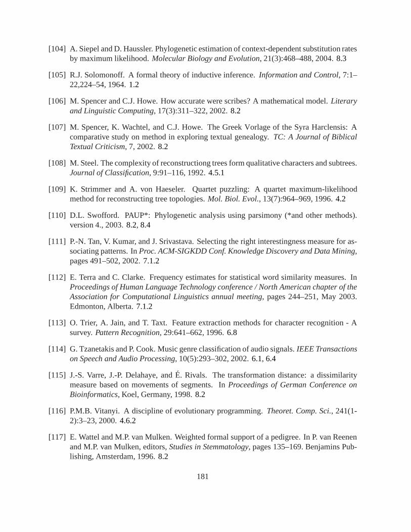
[104] A. Siepel and D. Haussler. Phylogenetic estimation ofcontext-dependent substitution ratesby maximum likelihood.Molecular Biology and Evolution, 21(3):468–488, 2004.8.3
[105] R.J. Solomonoff. A formal theory of inductive inference. Information and Control, 7:1–22,224–54, 1964.1.2
[106] M. Spencer and C.J. Howe. How accurate were scribes? A mathematical model.Literaryand Linguistic Computing, 17(3):311–322, 2002.8.2
[107] M. Spencer, K. Wachtel, and C.J. Howe. The Greek Vorlage of the Syra Harclensis: Acomparative study on method in exploring textual genealogy. TC: A Journal of BiblicalTextual Criticism, 7, 2002.8.2
[108] M. Steel. The complexity of reconstructiong trees form qualitative characters and subtrees.Journal of Classification, 9:91–116, 1992.4.5.1
[109] K. Strimmer and A. von Haeseler. Quartet puzzling: A quartet maximum-likelihoodmethod for reconstructing tree topologies.Mol. Biol. Evol., 13(7):964–969, 1996.4.2
[110] D.L. Swofford. PAUP*: Phylogenetic analysis using parsimony (*and other methods).version 4., 2003.8.2, 8.4
[111] P.-N. Tan, V. Kumar, and J. Srivastava. Selecting the right interestingness measure for as-sociating patterns. InProc. ACM-SIGKDD Conf. Knowledge Discovery and Data Mining,pages 491–502, 2002.7.1.2
[112] E. Terra and C. Clarke. Frequency estimates for statistical word similarity measures. InProceedings of Human Language Technology conference / North American chapter of theAssociation for Computational Linguistics annual meeting, pages 244–251, May 2003.Edmonton, Alberta.7.1.2
[113] O. Trier, A. Jain, and T. Taxt. Feature extraction methods for character recognition - Asurvey.Pattern Recognition, 29:641–662, 1996.6.8
[114] G. Tzanetakis and P. Cook. Music genre classification of audio signals.IEEE Transactionson Speech and Audio Processing, 10(5):293–302, 2002.6.1, 6.4
[115] J.-S. Varre, J.-P. Delahaye, and É. Rivals. The transformation distance: a dissimilaritymeasure based on movements of segments. InProceedings of German Conference onBioinformatics, Koel, Germany, 1998.8.2
[116] P.M.B. Vitanyi. A discipline of evolutionary programming. Theoret. Comp. Sci., 241(1-2):3–23, 2000.4.6.2
[117] E. Wattel and M.P. van Mulken. Weighted formal supportof a pedigree. In P. van Reenenand M.P. van Mulken, editors,Studies in Stemmatology, pages 135–169. Benjamins Pub-lishing, Amsterdam, 1996.8.2
181
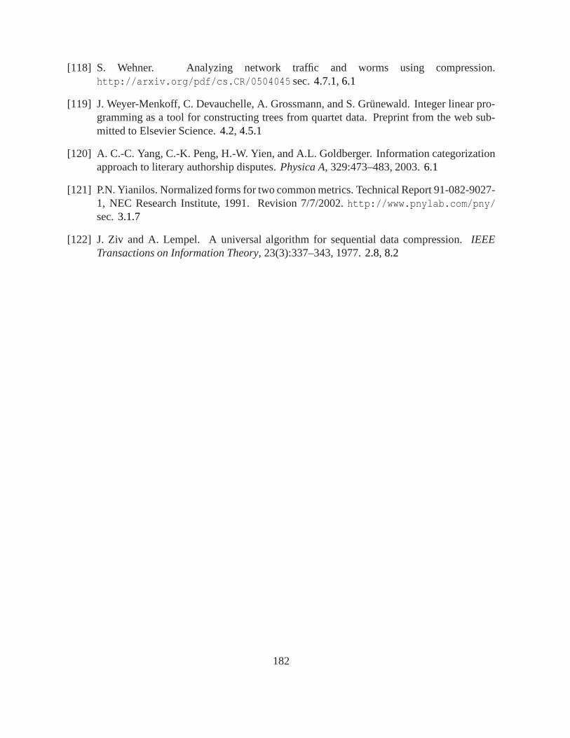
[118] S. Wehner. Analyzing network traffic and worms using compression.http://arxiv.org/pdf/cs.CR/0504045 sec.4.7.1, 6.1
[119] J. Weyer-Menkoff, C. Devauchelle, A. Grossmann, and S. Grünewald. Integer linear pro-gramming as a tool for constructing trees from quartet data.Preprint from the web sub-mitted to Elsevier Science.4.2, 4.5.1
[120] A. C.-C. Yang, C.-K. Peng, H.-W. Yien, and A.L. Goldberger. Information categorizationapproach to literary authorship disputes.Physica A, 329:473–483, 2003.6.1
[121] P.N. Yianilos. Normalized forms for two common metrics. Technical Report 91-082-9027-1, NEC Research Institute, 1991. Revision 7/7/2002.http://www.pnylab.com/pny/sec.3.1.7
[122] J. Ziv and A. Lempel. A universal algorithm for sequential data compression.IEEETransactions on Information Theory, 23(3):337–343, 1977.2.8, 8.2
182
Index
absolute,7, 26, 28, 108, 115abstract,16–18, 22, 107, 113according,146accuracies,132achieve,46, 111, 135adapt,29, 36adapts,29additive,21, 26–28, 30–32, 35adenovirus,63African, 98algorithm,23, 29, 36, 43, 45, 49, 51, 53–57,
59, 71, 72, 78, 139, 140, 142, 143,145, 147, 148, 153
algorithms,3, 32, 35, 36, 38, 53, 73–76, 92,145
alphabet,12–14, 17, 22, 26, 36, 37, 39, 60,79, 82, 113
American,98Amsterdam,26, 99, 102, 103ancestor,67, 93, 94Anglia, 138Anna,99, 100annealing,53, 143annotation,124anomaly,81approaching,109, 113approximate,3, 23, 31, 35, 39, 43, 45, 47,
51, 74, 77, 107, 109, 110, 112–114,134, 140
approximates,31, 36, 45, 53, 110, 141approximating,23, 31, 110, 116, 134arithmetic,22, 23, 25, 35–40array,5, 21, 79, 102artifact,82, 90artifacts,132ascomycetes,97, 98assertions,133assigning,5, 48, 110, 140atoms,143attracted,112, 122attribute,80, 131attributed,40, 153augment,14, 127authorship,80automate,75, 85automated,67, 93automatic,xx, 1, 58, 74–76, 79, 80, 105,
122, 124, 135, 136automating,64automaton,7auxiliary,44, 139avenues,44, 135Avogadro,120
Bach,57, 64, 86–90, 93Backgammon,124Balaenoptera,95balancing,45behave,39
183
belief,20Bennett,148Bernoulli,21, 36, 37, 39, 111best,144better,2, 67, 95bias,39, 73, 83, 110, 118, 145biased,22, 23, 109, 111, 114biases,111, 118Bibliography,9bifurcating,43, 44, 141–143, 148binary, xx, 3, 5, 12, 14, 15, 18, 26, 28, 30,
39, 45, 46, 49, 62, 72, 73, 82, 83,107, 110, 113, 124, 127, 136, 153
binned,56biology,67, 94, 139, 141, 142, 153bishop,137bishoprics,139black,100blue,146bootstrap,82, 96, 145, 151, 153bottom,103bound,11, 28, 32, 39, 83, 135boundary,29, 31, 75bovine,63box,144brackets,100breadth,2, 131brittle, 136bronchitis,63
calculation,17, 86, 108, 134cannibalized,87capability,74, 75, 134case,103caveats,131central,146century,138Ceratotherium,95certainty,7, 23, 48Chen,xixchess,7chimpanzee,95Christianization,138
clades,67, 94cladistics,139clarified,121clarify, 112class,103classifier,71–74, 102classify,64, 71, 73, 101, 102, 128, 130closer,26, 33, 62, 64, 87, 88, 90, 116closure,131cluster,3, 35, 43, 46, 54, 55, 57, 58, 62, 64,
79–82, 85, 88–90, 92, 101, 103, 111coder,36, 37, 39, 40codes,2, 11, 14–16, 22, 24codify, 7coding,3, 5, 11, 12, 14, 16, 22, 29, 31, 36,
37, 53, 64, 108, 111, 115, 119, 134cognition,134coin,11, 21–23, 52, 111, 134coincide,28, 144combine,9, 14, 71, 73combining,1, 2, 39, 71, 76compact,110comparison,xx, 40, 45, 69, 83, 96, 107, 130,
133, 137, 147, 149, 153, 154competing,94compiler,16, 17completeness,16complexity,xix, 11, 16, 18, 19, 21–24, 28–
31, 34–36, 43, 58, 80, 83, 92, 108–111, 115, 134, 140, 141, 143, 147,148
complicated,8, 19–21, 36, 91component,75, 76, 98, 127, 128composing,56, 145composite,14compress,1, 2, 29, 30, 36, 58, 73, 80, 84, 98,
105compressor,23, 25, 27–40, 58, 61, 62, 64,
68, 80, 83, 84, 95–99, 101, 102, 110–112, 115, 116, 134
compressors,1, 3, 5, 23, 25, 27–29, 31, 36,40, 41, 73, 79, 83, 84, 95, 102, 105,110–112, 140
184
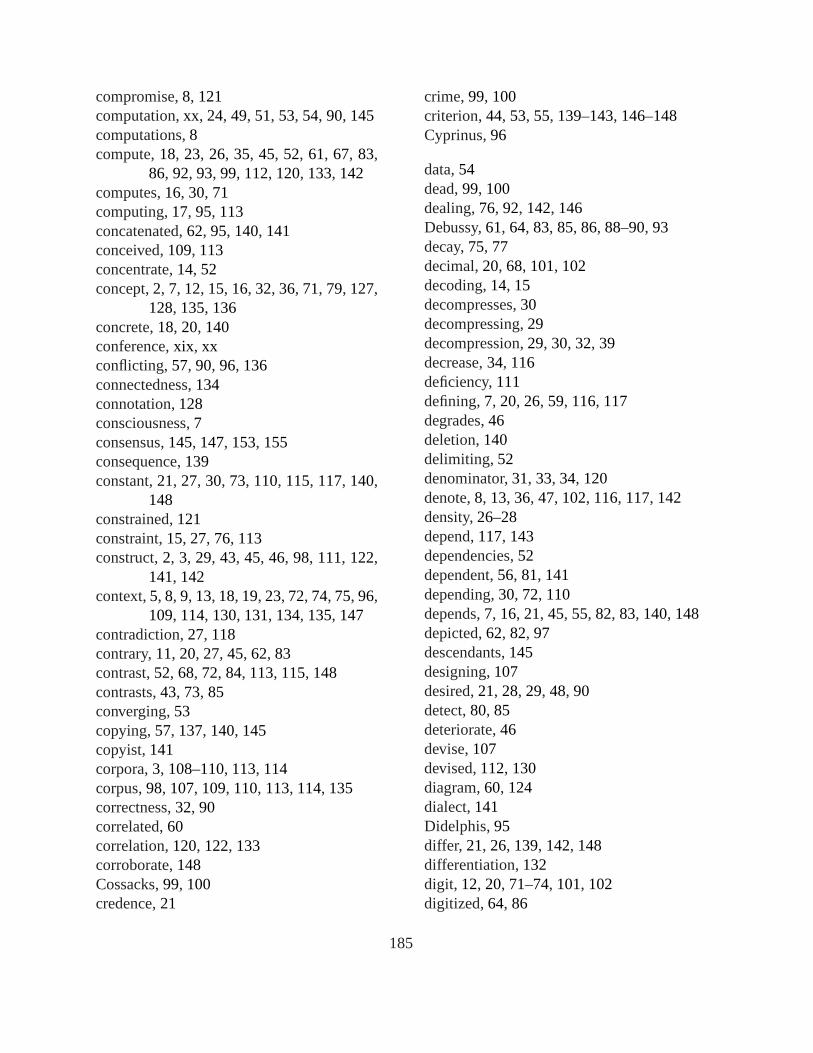
compromise,8, 121computation,xx, 24, 49, 51, 53, 54, 90, 145computations,8compute,18, 23, 26, 35, 45, 52, 61, 67, 83,
86, 92, 93, 99, 112, 120, 133, 142computes,16, 30, 71computing,17, 95, 113concatenated,62, 95, 140, 141conceived,109, 113concentrate,14, 52concept,2, 7, 12, 15, 16, 32, 36, 71, 79, 127,
128, 135, 136concrete,18, 20, 140conference,xix, xxconflicting,57, 90, 96, 136connectedness,134connotation,128consciousness,7consensus,145, 147, 153, 155consequence,139constant,21, 27, 30, 73, 110, 115, 117, 140,
148constrained,121constraint,15, 27, 76, 113construct,2, 3, 29, 43, 45, 46, 98, 111, 122,
141, 142context,5, 8, 9, 13, 18, 19, 23, 72, 74, 75, 96,
109, 114, 130, 131, 134, 135, 147contradiction,27, 118contrary,11, 20, 27, 45, 62, 83contrast,52, 68, 72, 84, 113, 115, 148contrasts,43, 73, 85converging,53copying,57, 137, 140, 145copyist,141corpora,3, 108–110, 113, 114corpus,98, 107, 109, 110, 113, 114, 135correctness,32, 90correlated,60correlation,120, 122, 133corroborate,148Cossacks,99, 100credence,21
crime,99, 100criterion,44, 53, 55, 139–143, 146–148Cyprinus,96
data,54dead,99, 100dealing,76, 92, 142, 146Debussy,61, 64, 83, 85, 86, 88–90, 93decay,75, 77decimal,20, 68, 101, 102decoding,14, 15decompresses,30decompressing,29decompression,29, 30, 32, 39decrease,34, 116deficiency,111defining,7, 20, 26, 59, 116, 117degrades,46deletion,140delimiting,52denominator,31, 33, 34, 120denote,8, 13, 36, 47, 102, 116, 117, 142density,26–28depend,117, 143dependencies,52dependent,56, 81, 141depending,30, 72, 110depends,7, 16, 21, 45, 55, 82, 83, 140, 148depicted,62, 82, 97descendants,145designing,107desired,21, 28, 29, 48, 90detect,80, 85deteriorate,46devise,107devised,112, 130diagram,60, 124dialect,141Didelphis,95differ, 21, 26, 139, 142, 148differentiation,132digit, 12, 20, 71–74, 101, 102digitized,64, 86
185
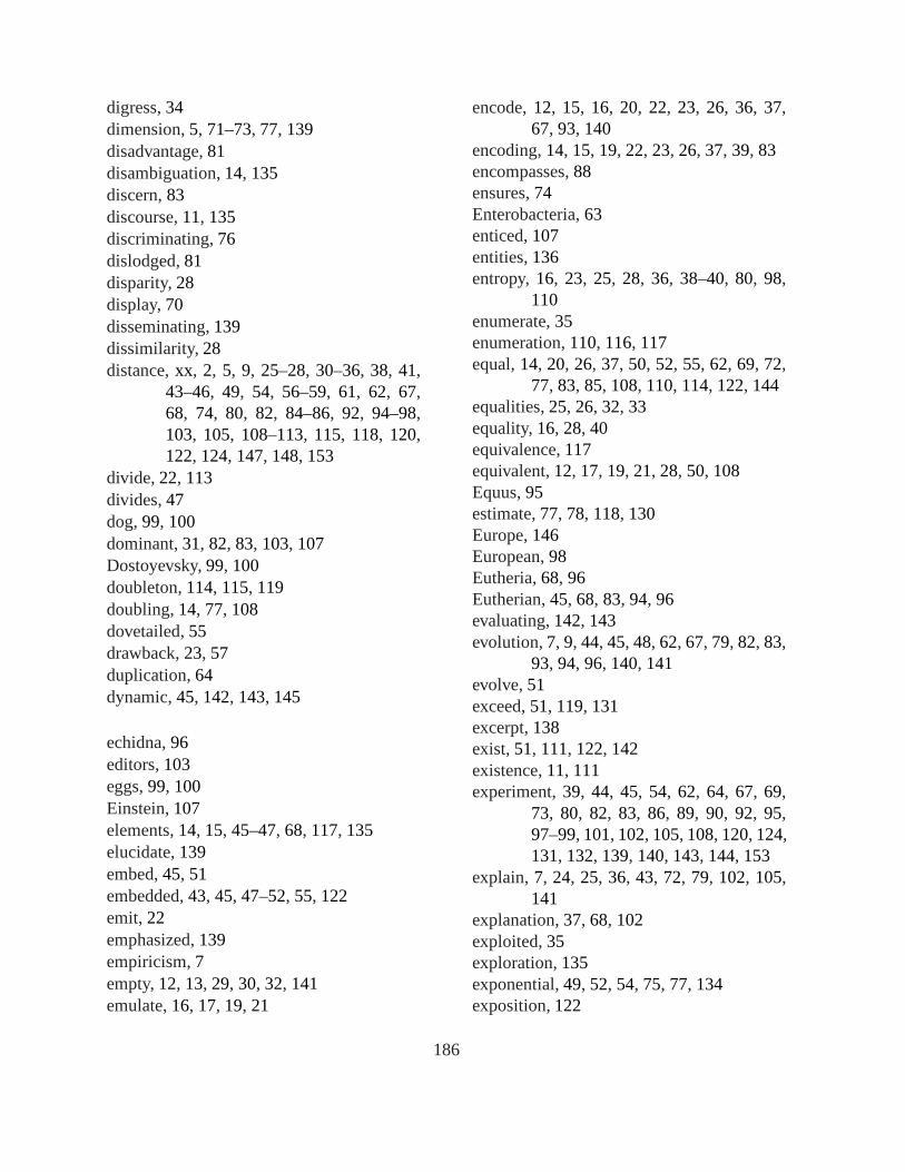
digress,34dimension,5, 71–73, 77, 139disadvantage,81disambiguation,14, 135discern,83discourse,11, 135discriminating,76dislodged,81disparity,28display,70disseminating,139dissimilarity,28distance,xx, 2, 5, 9, 25–28, 30–36, 38, 41,
43–46, 49, 54, 56–59, 61, 62, 67,68, 74, 80, 82, 84–86, 92, 94–98,103, 105, 108–113, 115, 118, 120,122, 124, 147, 148, 153
divide,22, 113divides,47dog,99, 100dominant,31, 82, 83, 103, 107Dostoyevsky,99, 100doubleton,114, 115, 119doubling,14, 77, 108dovetailed,55drawback,23, 57duplication,64dynamic,45, 142, 143, 145
echidna,96editors,103eggs,99, 100Einstein,107elements,14, 15, 45–47, 68, 117, 135elucidate,139embed,45, 51embedded,43, 45, 47–52, 55, 122emit,22emphasized,139empiricism,7empty,12, 13, 29, 30, 32, 141emulate,16, 17, 19, 21
encode,12, 15, 16, 20, 22, 23, 26, 36, 37,67, 93, 140
encoding,14, 15, 19, 22, 23, 26, 37, 39, 83encompasses,88ensures,74Enterobacteria,63enticed,107entities,136entropy,16, 23, 25, 28, 36, 38–40, 80, 98,
110enumerate,35enumeration,110, 116, 117equal,14, 20, 26, 37, 50, 52, 55, 62, 69, 72,
77, 83, 85, 108, 110, 114, 122, 144equalities,25, 26, 32, 33equality,16, 28, 40equivalence,117equivalent,12, 17, 19, 21, 28, 50, 108Equus,95estimate,77, 78, 118, 130Europe,146European,98Eutheria,68, 96Eutherian,45, 68, 83, 94, 96evaluating,142, 143evolution,7, 9, 44, 45, 48, 62, 67, 79, 82, 83,
93, 94, 96, 140, 141evolve,51exceed,51, 119, 131excerpt,138exist,51, 111, 122, 142existence,11, 111experiment,39, 44, 45, 54, 62, 64, 67, 69,
73, 80, 82, 83, 86, 89, 90, 92, 95,97–99, 101, 102, 105, 108, 120, 124,131, 132, 139, 140, 143, 144, 153
explain,7, 24, 25, 36, 43, 72, 79, 102, 105,141
explanation,37, 68, 102exploited,35exploration,135exponential,49, 52, 54, 75, 77, 134exposition,122
186
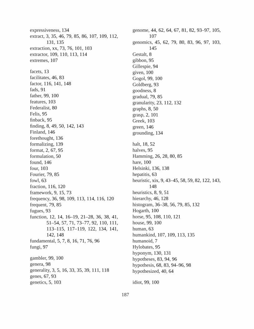
expressiveness,134extract,3, 35, 46, 79, 85, 86, 107, 109, 112,
131, 135extraction,xx, 73, 76, 101, 103extractor,109, 110, 113, 114extremes,107
facets,13facilitates,46, 83factor,116, 141, 148fads,91father,99, 100features,103Federalist,80Felis,95finback,95finding,8, 49, 50, 142, 143Finland,146forethought,136formalizing,139format,2, 67, 95formulation,50found,146four, 103Fourier,79, 85fowl, 63fraction,116, 120framework,9, 15, 73frequency,36, 98, 109, 113, 114, 116, 120frequent,79, 85fugues,93function,12, 14, 16–19, 21–28, 36, 38, 41,
51–54, 57, 71, 73–77, 92, 110, 111,113–115, 117–119, 122, 134, 141,142, 148
fundamental,5, 7, 8, 16, 71, 76, 96fungi, 97
gambler,99, 100genera,98generality,3, 5, 16, 33, 35, 39, 111, 118genes,67, 93genetics,5, 103
genome,44, 62, 64, 67, 81, 82, 93–97, 105,107
genomics,45, 62, 79, 80, 83, 96, 97, 103,145
Gestalt,8gibbon,95Gillespie,94given,100Gogol,99, 100Goldberg,93goodness,8gradual,79, 85granularity,23, 112, 132graphs,8, 50grasp,2, 101Greek,103green,146grounding,134
halt,18, 52halves,95Hamming,26, 28, 80, 85hare,100Helsinki,136, 138hepatitis,63heuristic,xix, 9, 43–45, 58, 59, 82, 122, 143,
148heuristics,8, 9, 51hierarchy,46, 128histogram,36–38, 56, 79, 85, 132Hogarth,100horse,95, 108, 110, 121house,99, 100human,63humankind,107, 109, 113, 135humanoid,7Hylobates,95hyponym,130, 131hypotheses,83, 94, 96hypothesis,68, 83, 94–96, 98hypothesized,40, 64
idiot, 99, 100
187
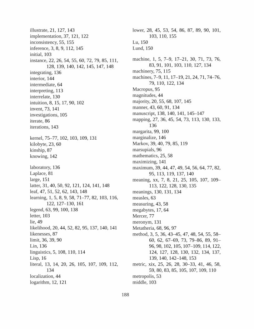
illustrate,21, 127, 143implementation,37, 121, 122inconsistency,55, 155inference,3, 8, 9, 112, 145initial, 103instance,22, 26, 54, 55, 60, 72, 79, 85, 111,
128, 139, 140, 142, 145, 147, 148integrating,136interior,144intermediate,64interpreting,113interrelate,130intuition, 8, 15, 17, 90, 102invent,73, 141investigations,105iterate,86iterations,143
kernel,75–77, 102, 103, 109, 131kilobyte,23, 60kinship,87knowing,142
laboratory,136Laplace,81large,151latter,31, 40, 50, 92, 121, 124, 141, 148leaf,47, 51, 52, 62, 143, 148learning,1, 5, 8, 9, 58, 71–77, 82, 103, 116,
122, 127–130, 161legend,63, 99, 100, 138letter,103lie, 49likelihood,20, 44, 52, 82, 95, 137, 140, 141likenesses,87limit, 36, 39, 90Lin, 136linguistics,5, 108, 110, 114Lisp, 16literal, 13, 14, 20, 26, 105, 107, 109, 112,
134localization,44logarithm,12, 121
lower, 28, 45, 53, 54, 86, 87, 89, 90, 101,103, 110, 155
Lu, 150Lund,150
machine,1, 5, 7–9, 17–21, 30, 71, 73, 76,83, 91, 101, 103, 110, 127, 134
machinery,75, 115machines,7–9, 11, 17–19, 21, 24, 71, 74–76,
79, 110, 122, 134Macropus,95magnitudes,44majority,20, 55, 68, 107, 145manner,43, 60, 91, 134manuscript,138, 140, 141, 145–147mapping,27, 36, 45, 54, 73, 113, 130, 133,
136margarita,99, 100marginalize,146Markov,39, 40, 79, 85, 119marsupials,96mathematics,25, 58maximizing,141maximum,39, 44, 47, 49, 54, 56, 64, 77, 82,
95, 113, 119, 137, 140meaning,xx, 7, 8, 21, 25, 105, 107, 109–
113, 122, 128, 130, 135meanings,130, 131, 134measles,63measuring,43, 58megabytes,17, 64Mercer,77meronym,131Metatheria,68, 96, 97method,3, 5, 36, 43–45, 47, 48, 54, 55, 58–
60, 62, 67–69, 73, 79–86, 89, 91–96, 98, 102, 105, 107–109, 114, 122,124, 127, 128, 130, 132, 134, 137,139, 140, 142–148, 153
metric, xix, 25, 26, 28, 30–33, 41, 46, 58,59, 80, 83, 85, 105, 107, 109, 110
metropolis,53middle,103
188
miniaturization,7minima,52minimum,8, 19, 21, 23, 44, 49, 50, 53, 73,
92, 140, 146, 147mining,1, 3, 9, 64, 81, 88, 91, 103, 161minus,33, 140misplaced,81misplacements,83, 98mixing, 23, 53monotremes,96Monte,53motivation,34MST, 92Murine,63mutation,51–53, 56, 141
naming,64native,98negative,32, 86, 116, 127, 128, 131, 134neighbor,76, 79, 82, 85, 95Netherlands,xvii , 97, 103NIST, 101, 102noise,120norm,28normalization,26, 148normalize,49, 115notable,7, 142notation,11, 12, 19, 21, 27noun,131novel,44, 58, 61, 83, 84, 109, 122Novosibirsk,64NP,44, 45, 49–51numbers,3, 5, 11, 12, 15, 21, 25, 28, 32, 47,
49, 52, 54, 86, 105, 108, 120, 122–124, 128, 136, 144, 151
numerator,31, 33, 34, 120, 148
obey,29object, 2, 18, 19, 21, 26, 28, 44, 53, 62,
71, 73, 81, 101, 102, 105, 107, 109,113, 115, 140, 153
objective,5, 11, 23, 57, 79, 108, 111, 116,122, 139
objectivity,112objects,xx, 2, 3, 5, 7, 9, 11, 12, 26, 28, 31,
34, 35, 43–46, 48, 49, 51, 54, 55, 57,58, 62, 71, 73, 74, 80, 82, 83, 87, 92,101–103, 105, 107–109, 112, 122,140
observer,9, 20obtain,27, 28, 34, 44, 45, 51, 52, 107, 109,
111, 114, 118, 119, 132occur,108, 111, 114, 120, 155occurrence,67, 80, 93, 105, 114, 115, 120omit, 39, 141ones,8, 12, 26, 28, 29, 46, 48, 50, 73, 79,
80, 85, 90, 92, 110, 137ontologies,135, 136ontology,122, 136opossum,95optima,143optimization,xix, 7, 44, 48, 51, 53, 75, 76optimizing,82, 122, 142, 143optimum,43, 45, 50–55, 147orangutan,95ordering,13, 18, 133, 153ordinal,13organisms,67, 94, 142oriented,139original,70Ornithorhynchus,95outcome,22, 23, 56, 60, 81, 82, 99outgoing,45, 83outline,73, 139output,2, 3, 14, 18, 19, 21–23, 44, 52, 55,
56, 67, 71–73, 76, 86, 90, 95, 124,149, 153
outset,8, 133over,54, 132overlap,115overlapping,40, 98overwriting,60
pairing,21, 90paleography,139paper,11, 102, 113, 139
189

paradox,92parallel,54, 55parameter,74, 75, 77, 78, 110, 116, 143paraphrased,130parse,14parsimony,82, 137, 140partial,19, 23, 143particular,103partition,47, 117PASCAL,xvii , xixpatching,145pattern,15, 25, 71, 79, 85, 139perceive,68, 81, 87perceived,64, 88periodicity,79, 85pertain,128phage,63phenomenon,8, 46, 55, 90, 92, 131, 145philologists,139Phoca,95photon,102phylogenies,81phylogeny,2, 43–45, 48, 58, 62, 67, 68, 80–
83, 93–96, 98, 108, 140, 145picking,60, 74, 141placental,67, 94, 96placentas,96plagiarism,58, 80, 91Plato,107platypus,95, 96plethora,3, 79, 109plotted,120polynomial,49, 51, 53pontifex,138portrait,99, 100possible,47preamble,37precision,26, 29, 31, 32, 51, 70precludes,107preconceived,83preconception,57, 83predicate,134, 135predicted,40
prediction,7, 23, 39, 72, 76preface,1, 14prefix,14–16, 18–20, 24, 26, 27, 30, 32, 53,
115–119, 124preliminary,xix, 137prima,138primates,68, 95, 96primes,128primitive,134Princeton,136probability,3, 8, 11, 12, 16, 21–23, 37, 39,
40, 44, 52, 53, 55, 81, 110, 111,113–122, 134, 141, 143
probable,60, 81, 114, 146processing,61, 82, 83, 85procreate,96program,154programmers,135programming,16, 17, 19, 45, 51, 54, 58–60,
76, 80, 135, 136, 142, 143, 145prophetess,124proportion,1, 20, 21, 56, 119proportional,134, 141protocol,105, 136Prototheria,68, 96proximity, 62, 97pseudo,59, 60, 112psychology,108punishment,99, 100purpose,70puzzling,43, 44, 49pygmy,95
quantification,15, 45quantify,44, 145quantities,40, 73, 86quantized,86quarrelled,99, 100Quine,7quotient,38
radial,75, 77randomized,44, 45, 51, 55, 82, 122
190
randomness,20, 22, 92rarefied,7ratio,20, 21, 33, 39, 148rationale,48ratios,2, 102razor,140rearrange,30rearrangements,67, 93recapitulating,122recoded,26, 82reduction,50, 76referees,103references,140regularity,20, 101relative,13, 26–29, 31, 33, 37, 48, 49, 69,
98, 108–110, 113, 114, 134relativized,110relevance,111rely, 13remainder,9, 43remains,33, 34, 143, 145remark,86removes,134repeat,30, 44, 78repetitions,29, 60, 111rephrase,49replacing,141repositories,61, 83requirement,27, 118rescale,49researchers,97, 102, 139resemble,57restriction,24, 142, 146resultant,121revealing,134rewrite,30, 33rewritten,31, 40, 115, 141robustness,3, 5, 64, 102, 105, 109rodents,68, 95–97rough,71, 76, 131, 137, 149rounding,24, 37, 112row, 101, 112rows,133
Russian,99, 100
Saccharomyces,97, 98Saccharomycetaceae,98SARS,63satisfied,118satisfies,14, 15, 26–28, 30, 32, 33, 76, 77satisfy,27–29, 50, 116, 119, 120scalar,76scaling,68, 69, 76, 92scanning,72, 74, 101scenarios,145schema,136scheme,14, 22, 23, 36, 51–53, 72, 136Schubert,91segment,142–144semantics,xx, 109, 110, 114–116, 118, 128,
130semi,1, 75, 110, 135sentence,112sequel,45, 82, 109, 114sequence,2, 11–15, 17–23, 36, 40, 51–53,
60, 64, 71–73, 81, 96, 111, 112, 130,133, 153
Shannon,16, 21, 22, 28, 36, 37, 40, 80, 110,111, 113, 134
shorthand,18showing,138, 152signals,86significance,1, 138similarities,44, 58, 79, 80, 85, 89, 91, 92,
107, 111, 152similarity, xix, xx, 2, 25–28, 31, 33–35, 41,
46, 58, 62, 64, 79, 80, 83, 85, 88,90, 102, 103, 107–109, 115
simplifications,103simplifies,17, 122simplify, 73simplifying,121simulate,17singleton,114, 115, 119, 120smoothness,45snapshot,9, 115, 161
191

Socrates,107solve,3, 5, 136, 139, 142sons,99, 100spanning,92species,2, 67, 95spectrum,5, 102splice,141spreading,44Springer,xixstability,56stabilize,108stable,92, 116standardization,136static,36–40statistic,96stemmata,139, 145stemmatics,139stemmatology,xx, 137, 139, 140steps,40, 45, 52, 54–56, 87, 94, 121, 153stored,17, 111stress,68strings,11–15, 18, 20, 23, 24, 26, 29, 30, 32,
34, 37, 84, 107, 111, 112, 115, 121,132, 140, 142, 147, 148
structure,45, 47, 51, 89, 97, 105, 120, 130,134, 136, 141–143, 146, 149
studying,87subgroup,151subjectivity,112subsection,109subset,48, 114, 117substitution,34, 35subsumed,95, 118subsumes,26subtracting,33, 34subtraction,35suffix, 23, 32Sumatran,95superimposes,99supervised,122suppositions,81symbol,12, 13, 17–19, 36, 37, 40, 71, 72,
105
symmetry,26, 29–32, 34, 35, 81synonym,130synset,130, 131syntax,121
table,146Tachyglossus,96tail, 52, 53, 56Taras,99, 100task,5, 48, 73, 75, 101, 102taxonomy,62, 97technique,1, 64, 73, 76, 77, 101, 103, 135,
153telegrams,111temporal,45, 64, 83terminology,9, 110terms,103ternary,45, 46, 51, 57, 59, 62, 83, 97, 122theories,3, 7, 108, 153, 155theory,xx, 1, 3, 5, 8, 11, 21–24, 29–31, 34,
44, 58, 76, 80, 82, 85, 102, 105, 108,109, 111, 113, 121, 134
thesis,xvii , xix, xx, 1–3, 5, 7, 9, 11–13, 15,16, 18, 57, 58, 61, 71, 74, 80–82,108, 122, 130, 161
three,47tokens,112Tolstoy,99, 100, 105, 107tradeoff,55transitivity,50translator,100traverse,131tree,2, 48, 59, 61, 67, 84, 95, 103, 123, 144,
146, 151, 152trees,2, 3, 5, 23, 44, 45, 47, 49–56, 62, 67,
80, 82, 83, 92, 93, 95, 96, 122, 124,137, 141–146, 148, 149, 151, 153,161
trillions, 107truncated,68, 70Turgenev,99, 100Turing,11, 16–21, 24, 30, 31, 110, 134two, 99, 100, 151
192
type,63typos,103
ubiquity,111underlining,139underlying,5, 8, 12, 16, 45, 46, 58, 80, 92,
103, 105, 112, 115, 120, 140uniformity, 14universal,7, 16–22, 24, 30, 31, 34, 62, 74–
76, 80, 85, 97, 98, 107, 109, 110,113, 116–118, 134, 135
universality,25, 28, 31, 34, 62, 81, 83, 105,109, 110, 118, 119
universe,143university,138unknown,xix, 1, 5, 9, 35, 71, 73, 77, 79, 83,
88, 91, 92, 102, 103, 133, 143unlearn,29unpredictability,128Uppsala,137, 150US,63using,2, 6, 67, 95, 97, 123, 156–159utterances,134
validation,74, 75, 77–79, 131validity, 148values,19, 28, 40, 43–45, 49, 52, 55, 58, 68,
69, 80, 82, 86, 96, 113, 124, 131,133, 142, 153
variability, 81, 102vastness,108vector,5, 7–9, 71–76, 98, 101, 103, 122, 127vectors,71, 73, 76, 77, 79, 80, 85, 101–103,
109, 127, 131veracity,98verification,8, 64Verticillium, 97viewpoint,36, 110virus,63visualization,1, 3, 5, 103vocabulary,105, 132, 133vowel,112
war,99, 100
wavelet,79, 85well, 2, 61, 67, 84, 95wise,33, 82, 98, 145wolf, xvii , xix, 103WordNet,xx, 105, 128, 130–132, 134–136words,xx, 7, 14–16, 57, 80, 99, 105, 107,
109, 110, 112–115, 121, 122, 127,128, 130–133, 135, 141, 142, 144–146, 150
workstations,54writers,6, 99, 100, 156–159
yeasts,97yellow, 146yielding,56
zero,22, 53, 121, 122, 141–143, 146
193

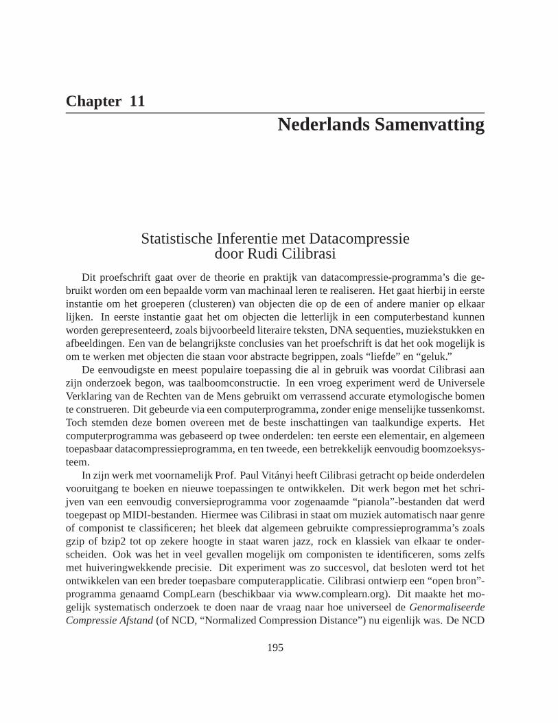
Chapter 11
Nederlands Samenvatting
Statistische Inferentie met Datacompressiedoor Rudi Cilibrasi
Dit proefschrift gaat over de theorie en praktijk van datacompressie-programma’s die ge-bruikt worden om een bepaalde vorm van machinaal leren te realiseren. Het gaat hierbij in eersteinstantie om het groeperen (clusteren) van objecten die op de een of andere manier op elkaarlijken. In eerste instantie gaat het om objecten die letterlijk in een computerbestand kunnenworden gerepresenteerd, zoals bijvoorbeeld literaire teksten, DNA sequenties, muziekstukken enafbeeldingen. Een van de belangrijkste conclusies van het proefschrift is dat het ook mogelijk isom te werken met objecten die staan voor abstracte begrippen, zoals “liefde” en “geluk.”
De eenvoudigste en meest populaire toepassing die al in gebruik was voordat Cilibrasi aanzijn onderzoek begon, was taalboomconstructie. In een vroeg experiment werd de UniverseleVerklaring van de Rechten van de Mens gebruikt om verrassendaccurate etymologische bomente construeren. Dit gebeurde via een computerprogramma, zonder enige menselijke tussenkomst.Toch stemden deze bomen overeen met de beste inschattingen van taalkundige experts. Hetcomputerprogramma was gebaseerd op twee onderdelen: ten eerste een elementair, en algemeentoepasbaar datacompressieprogramma, en ten tweede, een betrekkelijk eenvoudig boomzoeksys-teem.
In zijn werk met voornamelijk Prof. Paul Vitányi heeft Cilibrasi getracht op beide onderdelenvooruitgang te boeken en nieuwe toepassingen te ontwikkelen. Dit werk begon met het schri-jven van een eenvoudig conversieprogramma voor zogenaamde“pianola”-bestanden dat werdtoegepast op MIDI-bestanden. Hiermee was Cilibrasi in staat om muziek automatisch naar genreof componist te classificeren; het bleek dat algemeen gebruikte compressieprogramma’s zoalsgzip of bzip2 tot op zekere hoogte in staat waren jazz, rock enklassiek van elkaar te onder-scheiden. Ook was het in veel gevallen mogelijk om componisten te identificeren, soms zelfsmet huiveringwekkende precisie. Dit experiment was zo succesvol, dat besloten werd tot hetontwikkelen van een breder toepasbare computerapplicatie. Cilibrasi ontwierp een “open bron”-programma genaamd CompLearn (beschikbaar via www.complearn.org). Dit maakte het mo-gelijk systematisch onderzoek te doen naar de vraag naar hoeuniverseel deGenormaliseerdeCompressie Afstand(of NCD, “Normalized Compression Distance”) nu eigenlijk was. De NCD
195
is een afstandsmaat tussen bestanden die aangeeft in hoeverre twee bestanden op elkaar lijken.Verschillende datacompressoren leiden tot verschillendeversies van deze afstandsmaat.
In het eerste belangrijke artikel, Clustering by Compression (Groeperen met Compressie),ontwikkelden Vitányi en Cilibrasi een methode om aannames over datacompressoren te formalis-eren, en beschreven zij enkele formele eigenschappen van zowel de theoretische “KolmogorovComplexiteit compressor” als van praktische, daadwerkelijk toepasbare compressoren. Vervol-gens pasten zij het CompLearn systeem toe op genetische analyse waarbij zij gebruik makenvan complete genoomsequenties. Dit gebeurde wederom zonder enige biologische aannamesof menselijke tussenkomst, hetgeen leidde tot de veronderstelling dat de methode enigszinsobjectiever was dan eerdere, vergelijkbare pogingen. Verder paste Cilibrasi CompLearn enNCD toe op een probleem in de radioastronomie, een domein waarvan hij bijna niets afwist.Gelukkig kwamen de resultaten overeen met die van in de nabijheid werkende astromische ex-perts. Toepassing van het programma op vertaalde Russischeliteratuur toonde dat het boekengroepeerde aan de hand van een combinatie van vertaler en originele auteur. Misschien het meestverrassende resultaat werd bereikt bij het experiment waarbij afbeeldingen herkend moesten wor-den: het bleek mogelijk om het standaard compressieprogramma gzip te gebruiken voor hetidentificeren van afbeeldingen van handgeschreven cijfersuit een NIST gegevensbank. Cilibrasiwerkte deze toepassing verder uit door het combineren van deNCD met zogenaamde SupportVector Machines. Dit zijn zelflerende systemen (algoritmen) die elke continue functie kunnenleren. De matrix van NCD afstanden tussen een groep “trainings”-bestanden en een aantal van tevoren gekozen “anker”-bestanden werd hier gebruikt als input voor de support vector machine.Het resultaat is een algemeen classificatie- en regressieprogramma dat de kracht van discretepatroonvergelijking in datacompressoren combineert met de flexibiliteit van universeel lerendeautomaten van continue functies zoals Support Vector Machines of neurale netwerken.
De volgende grote vernieuwing kwam toen Cilibrasi zich realiseerde dat we dezelfde wiskun-dige formalismen die ten grondslag liggen aan datacompressie ook kunnen toepassen op andereobjecten dan bestanden (of reeksen van bits). Het domein zoubijvoorbeeld ook uit zoekter-men of tupels van zoektermen kunnen bestaan. Men kan dan een zoekmachine zoals Googlegebruiken om het aantal pagina’s op het world wide web te bepalen waarin deze (tupels van)zoektermen voorkomen. Het resultaat is dan de zogenaamde “genormaliseerde Google afstand”(NGD), die voor twee willekeurige termen (bijvoorbeeld woorden) aangeeft hoeveel ze, volgenshet world wide web, op elkaar lijken. De NGD werd geimplementeerd als onderdeel van deCompLearn software met het zogenaamde Simple Object AccessProtocol (SOAP) met de Cen Ruby programmeertalen. Het grote verschil met NCD is dat het nu mogelijk is om afstandte bepalen op basis van denamenvan objecten in plaats van hun, statistisch genomen, letter-lijke inhoud. Dit bracht een scala aan nieuwe mogelijkhedenteweeg. Cilibrasi vergeleek au-tomatisch gegenereerde monsters van ontologische predicaten met die van WordNet, een projectvan de universiteit van Princeton. WordNet is een semantische concordantie van de Engelsetaal die is gebouwd door menselijke experts. Er was ongeveer85% overeenstemming tussende eenvoudige, volledige automatisch lerende automaat en WordNet. Dit maakt automatischeontologie-uitbreiding een veelbelovende onderzoeksrichting. Hiermee zou als het waregratisstructuur aangebracht kunnen worden in het web; dit in tegenstelling tot een meer traditioneleaanpak met RDF tripletten, het Sematische Web en XML uitwisseling. Al deze methoden
196

vereisen zeer tijdrovende menselijke arbeid, terwijl de nieuwe, op de NGD gebaseerde tech-nieken, moeiteloos soortgelijke kennis vergaren uit het grote, ongebruikte reservoir van reedsbestaande webpagina’s. Een ander interessant experiment was een automatisch Engels-Spaansvertaalsysteem dat werkte zonder menselijke hulp. Cilibrasi was in staat om de Spaanse vertalin-gen van vijf Engelse woorden door elkaar te husselen en de computer te laten uitvogelen welkeEngelse en Spaanse woorden overeenstemden. Slechts door decorrelatie tussen de Engelse NGDmatrix en alle Spaanse permutaties te berekenen, lukte het de juiste volgorde te vinden.
In het meest recente artikel over Cilibrasi’s onderzoek, bepaalden Cilibrasi en Vitányi dewiskundige details van het exacte type niet-deterministisch kwartetboomzoeksysteem dat hijuiteindelijk bouwde. Dit bleek een interessant project te zijn vanuit het oogpunt van de algo-ritmiek: het is een NP-hard probleem om de beste boom te bepalen volgens het gebruikte eval-uatiecriterium, maar desalniettemin bleek het mogelijk voor vele interessante en bruikbare voor-beelden het antwoord te benaderen met een verrassende mate van snelheid en precisie. Daarbijmaakte Cilibrasi gebruik van een cluster-berekenend systeem dat gebouwd was volgens de zoge-naamde Message Passing Interface (MPI) standaard. Een voorbeeld dat Cilibrasi op dit momentzeer interesseert is een boom van 100 verschillende monsters van het vogelgriepvirus. Terwijlmutaties en recombinaties nieuwe virale variaties vormen,is het systeem in staat gebleken snelleen nuttige antwoorden te geven.
Cilibrasi moedigt geïnteresseerden aan de artikelen te bekijken die gepubliceerd zijn op zijnonderzoeks-homepage, of de online demo te proberen op de CompLearn website. Er kan ook een3D demo gedownload worden met sleur-en-pleur-datamining.Windows en linux versies van alleprogrammatuur zijn tevens beschikbaar. Mede door een verbinding te maken met ongeveer 15andere programmatuursystemen, heeft Cilibrasi een stuk gereedschap geproduceerd dat waarde-vol kan zijn voor onderzoekers over de hele wereld.
197

Chapter 12
Biography
Rudi Cilibrasi was born in Brooklyn, New York in 1974. He moved west to California at anearly age and grew up in Sacramento mostly in front of a computer. He eventually went southto Pasadena where he attended the California Institute of Technology and received a degree inEgineering and Applied Sciences with a specialization in Computer Science. He contributedto an early version of the Linux kernel as an open-source programmer. After graduating hespent some years in industry and enjoyed developing programming skills in data compressionalgorithms, networking, cryptography, computer graphics, and artificial intelligence algorithmsof all stripes. He returned to school after the dot-com crashand joined CWI in 2001 as a PhDstudent. After being awarded his doctoral degree he will focus more on his chosen interests: as anopen source programmer he created CompLearn. CompLearn is an innovative machine learningsystem that leverages data compression programs for statistical analysis. He has also been activeas a Hepatitis C advocate and activist, calling attention tothis and a variety of other publichealth issues. He has been involved in community disaster response and emergency governance,helping to create both the TsunamiHelp.info wiki as well as the KatrinaHelp.info wiki after theseunprecedented disasters. Rudi has a passion for striving for perfection in programming processand is a heavy proponent of the Agile Development camp; in recent years he has forgotten mostof his C++ and Java knowledge to strengthen his focus on C and Ruby, which he believes holdpromise for a new era of software reliability and power.
Papers by R. Cilibrasi
1. R. Cilibrasi, P.M.B. Vitanyi, A New Quartet Tree Heuristic for Hierarchical Clustering,IEEE/ACM Trans. Computat. Biol. Bioinf., Submitted; and was presented at the EU-PASCAL Statistics and Optimization of Clustering Workshop, 5-6 Juli 2005, London, UK.http://arxiv.org/abs/cs.DS/0606048
2. J. Tromp, R. Cilibrasi, The Limits of Rush-Hour Complexity, March 23, 2006.http://arxiv.org/pdf/cs.CC/0502068.
199

3. R. Cilibrasi, R. de Wolf, P. Vitanyi. Algorithmic clustering of music based on string com-pression,Computer Music J., 28:4(2004), 49-67.
4. R. Cilibrasi, P. Vitanyi. Automatic Extraction of Meaning from the Web. IEEE Interna-tional Symposium on Information Theory, Seattle, Washington, 2006.
5. R. Cilibrasi, P. Vitanyi. Clustering by compression,IEEE Trans. Information Theory,51:4(2005), 1523 - 1545.
6. R. Cilibrasi, L. van Iersel, S. Kelk, J. Tromp. On the Complexity of Several HaplotypingProblems. Proc. WABI 2005: 128-139
7. R. Cilibrasi, L. van Iersel, S. Kelk, J. Tromp. On the complexity of the Single IndividualSNP Haplotyping Problem, Algorithmica,To appear.http://arxiv.org/pdf/q-bio.GN/0508012.
8. T.Roos, T.Heikki, R.Cilibrasi, P.Myllymaki. Compression-based Stemmatology: A Studyof the Legend of St. Henry of Finland, (number HIIT-2005-3),2005.
9. R. Cilibrasi, P. Vitanyi. Similarity of Objects and the Meaning of Words,Proc. 3rd Conf.Theory and Applications of Models of Computation (TAMC), 15-20 May, 2006, Beijing,China. Lecture Notes in Computer Science, Vol. 3959, Jin-YiCai, S. Barry Cooper, andAngsheng Li (Eds.), 2006, 21–45.
10. R. Cilibrasi Domain Independent Hierarchical ClusteringNieuwsbrief van de NederlandseVereniging voor Theoretische Informatica, 2004, nummer 8.
11. R. Cilibrasi, P. Vitanyi. The Google similarity distance, IEEE/ACM Transactions onKnowledge and Data Engineering, To appear.
12. R. Cilibrasi, Zvi Lotker, Alfredo Navarra, Stephane Perennes, Paul Vitanyi.Lifespan ofPeer to Peer Networks: Models and Insight, 10th International Conference On PrinciplesOf Distributed Systems (OPODIS 2006), December 12-15, 2006, Bordeaux Saint-Emilion,France.
200

Titles in the ILLC Dissertation Series:
ILLC DS-2001-01:Maria AloniQuantification under Conceptual Covers
ILLC DS-2001-02:Alexander van den BoschRationality in Discovery - a study of Logic, Cognition, Computation and Neuropharmacology
ILLC DS-2001-03:Erik de HaasLogics For OO Information Systems: a Semantic Study of Object Orientation from a Cate-gorial Substructural Perspective
ILLC DS-2001-04:Rosalie IemhoffProvability Logic and Admissible Rules
ILLC DS-2001-05:Eva HooglandDefinability and Interpolation: Model-theoretic investigations
ILLC DS-2001-06:Ronald de WolfQuantum Computing and Communication Complexity
ILLC DS-2001-07:Katsumi SasakiLogics and Provability
ILLC DS-2001-08:Allard TammingaBelief Dynamics. (Epistemo)logical Investigations
ILLC DS-2001-09:Gwen KerdilesSaying It with Pictures: a Logical Landscape of Conceptual Graphs
ILLC DS-2001-10:Marc PaulyLogic for Social Software
ILLC DS-2002-01:Nikos MassiosDecision-Theoretic Robotic Surveillance
ILLC DS-2002-02:Marco AielloSpatial Reasoning: Theory and Practice
ILLC DS-2002-03:Yuri EngelhardtThe Language of Graphics
ILLC DS-2002-04:Willem Klaas van DamOn Quantum Computation Theory
ILLC DS-2002-05:Rosella GennariMapping Inferences: Constraint Propagation and Diamond Satisfaction
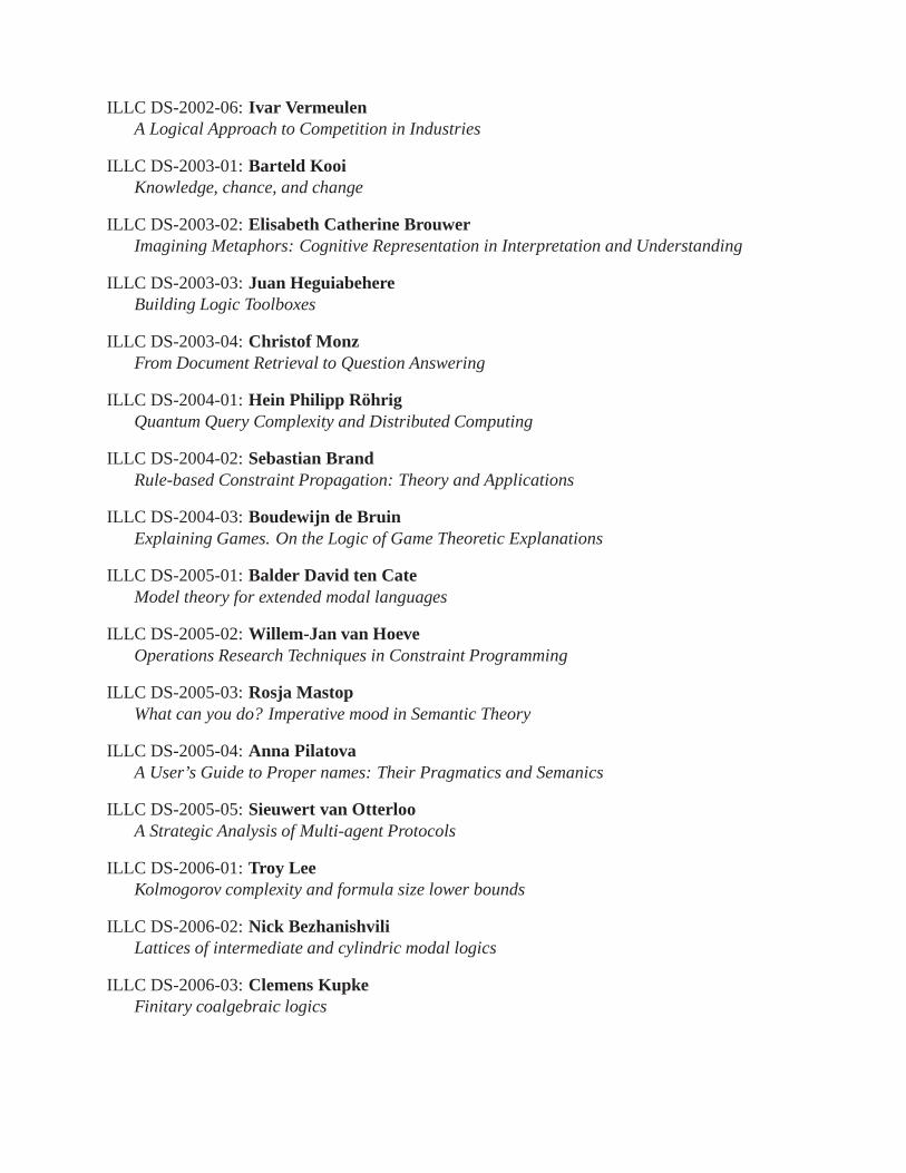
ILLC DS-2002-06:Ivar VermeulenA Logical Approach to Competition in Industries
ILLC DS-2003-01:Barteld KooiKnowledge, chance, and change
ILLC DS-2003-02:Elisabeth Catherine BrouwerImagining Metaphors: Cognitive Representation in Interpretation and Understanding
ILLC DS-2003-03:Juan HeguiabehereBuilding Logic Toolboxes
ILLC DS-2003-04:Christof MonzFrom Document Retrieval to Question Answering
ILLC DS-2004-01:Hein Philipp RöhrigQuantum Query Complexity and Distributed Computing
ILLC DS-2004-02:Sebastian BrandRule-based Constraint Propagation: Theory and Applications
ILLC DS-2004-03:Boudewijn de BruinExplaining Games. On the Logic of Game Theoretic Explanations
ILLC DS-2005-01:Balder David ten CateModel theory for extended modal languages
ILLC DS-2005-02:Willem-Jan van HoeveOperations Research Techniques in Constraint Programming
ILLC DS-2005-03:Rosja MastopWhat can you do? Imperative mood in Semantic Theory
ILLC DS-2005-04:Anna PilatovaA User’s Guide to Proper names: Their Pragmatics and Semanics
ILLC DS-2005-05:Sieuwert van OtterlooA Strategic Analysis of Multi-agent Protocols
ILLC DS-2006-01:Troy LeeKolmogorov complexity and formula size lower bounds
ILLC DS-2006-02:Nick BezhanishviliLattices of intermediate and cylindric modal logics
ILLC DS-2006-03:Clemens KupkeFinitary coalgebraic logics

ILLC DS-2006-04:Robert ŠpalekQuantum Algorithms, Lower Bounds, and Time-Space Tradeoffs
ILLC DS-2006-05:Aline HoninghThe Origin and Well-Formedness of Tonal Pitch Structures
ILLC DS-2006-06:Merlijn SevensterBranches of imperfect information: logic, games, and computation
ILLC DS-2006-07:Marie NilsenovaRises and Falls. Studies in the Semantics and Pragmatics of Intonation


