82
Statistical Methods and Their Applications

Statistical Methods and Their Applications

Session 2. Statistical Methods and Their Applications
70
STATISTICAL MODELLING OF TRUCKS’ WORK ON THE INTERNATIONAL ROUTES AT VARIOUS STRATEGY
RETURN LOADING ACCEPTANCE
Sergey Azemsha
Belarusian State University of Transport Kirov street 34, Gomel, Belarus, 246022
E-mail: [email protected]
Characteristic feature of the international automobile cargoes transportations is the great value of vehicles run on a route. To evaluate efficiency of the given kind of transportations it is necessary to pay a special attention to the process of search and choice return loadings. The problem of cargoes in passing (the return passing) a direction is partially solved, that is connected with development of transport portals at Internet. However the problem of a choice rational transportation from set of alternative loadings variants remains actually. The decision on acceptance of this or that cargo to transportation now is accepted by carriers managers on the basis of the intuitive conclusions based on personal practical experience. As a rule, such a strategy of decision-making on a choice of rational return transportation is reduced to – the truck by transporting cargo has minimal waiting time.
There is offered new, based on processing of the statistical information, strategy of decision-making on a choice of rational return transportation in the given article,. The offered strategy of decision-making is based on the basis of the analysis more than 850 routes of trucks’ work on a direction Byelorussia-the Russian Federation. Statistical modelling of the cargo automobile work on each offered strategy and the subsequent economic estimation of the executed transportations allows defining optimum strategy of decision-making.
Keywords: strategy of decision-making, modelling work of automobile vehicles, rational transportation, the law of distribution
1. INTRODUCTION The problem to increase the efficiency of automobile cargoes transportations has the high
importance in the developed conditions of a rigid competition in the market of transport services. To increase effect from the carried out transportation process it is obviously possible due to increase in a degree of use of run and carrying capacity of vehicles. The specialized information resources created in INTERNET contain the information on cargoes shown to transportation. It enables to solve a task in view – enables to prospect cargoes with the purpose of improvement of parameters of vehicles work. However the problem of a choice the optimum transportation from a set of the cargoes offered to transportation remains actual. In practice the given problem is solved on the basis of acceptance of the intuitive decisions based on practical experience of activity auto carriers managers. Thus it is accepted to minimize an idle time of a vehicle pending return loading, and as financial criterion of acceptance of this or that cargo to transportation the size of the rate of the freight acts for transportation not below average on the given direction. Such approach to maintenance and a choice of return loading is represented, not always proved. For the decision of the stated problem it is necessary to develop and prove expediency application of various techniques of decision-making at the choice of rational transportation, and to choose the optimum from them.
2. THE OVERALL PERFORMANCE CRITERION OF TRUCKS
As the criterion, allowing making the comparative analysis various variants of transportations,
in the lead researches the specific profit [1] is offered. This parameter is defined as the attitude of the profit received by an automobile carrier from performance of this or that transportation, to time spent for its performance, and carrying capacity of a vehicle. The given parameter shows, what profit is brought with an automobile vehicle in unit of time on unit of the carrying capacity. In the developed kind expression of specific profit has the following:
qS
))TTt(tβVq(L)dТ)Sd(β(LV
P const
eitclutfr
ititsfrts −
++++⋅+−⋅
= var , (1)

The 7th International Conference “RELIABILITY and STATISTICS in TRANSPORTATION and COMMUNICATION - 2007”
71
where tV – technical speed of movement of a vehicle; frL – run of an automobile vehicle with a cargo, during job on a route;
β – operating ratio of run of an automobile vehicle; sd – specific proceeds for a unit of run. It depends on carrying capacity of an automobile
vehicle demanded for transportation and can be approximated by linear dependence dsss qаad 10 += ; varS – variable expenses for a unit of run. These expenses depend on carrying capacity of a
vehicle and its actual use and can be expressed as )βγaq(аaS stvar2var1var0var 1 ++= ; itT – expected paid time of the above permitted standard idle time under cargo operations in
fault of the customer; itd – payment for a time unit of the above permitted standard idle time under cargo operations
in fault of the customer. It can be presented also by linear dependence on carrying capacity of a demanded automobile vehicle dititit qаad 10 += ;
lut – standard time of loading-unloading of an automobile vehicle; ct – expected duration of idle time at the control and documentary registration of transportation
(at customs, etc.); constS – constant expenses for a time unit of job. These expenses depend basically on carrying
capacity of an automobile vehicle qаaS constconstconst 10 += ; eT – prospective duration of expectation of passing loading; dq – carrying capacity of the demanded (declared) automobile vehicle ( qqd ≤ ).
It is established, that operated parameters in specific profit expression are full run, operating ratio of the run, demanded carrying capacity and a waiting time of return loading [2]. Besides it has been shown, that between operated parameters there is a statistical connection [3, 4]. It is caused by that with increase in a waiting time of return loading the quantity of the cargoes offered to transportation in the necessary direction extends. Having found dependence of length on a run with cargo, operating ratio of run and demanded carrying capacity from a waiting time of return loading, and substituting them in expression of specific profit, after differentiation of expression (1), it is possible to receive, that an optimum waiting time of return loading is equally 15 hours [3].
3. THE STRATEGY OF DECISION-MAKING ON THE CHOICE
OF RATIONAL RETURN TRANSPORTATION DEVELOPMENT As one of decision-making strategy on a choice of rational return transportation there will be a
strategy based on occurrence expectation of a return cargo till 15 o'clock. In the lead researches connection between a waiting time of occurrence by a vehicle of the shipping request of a cargo which will allow reaching the maximal value of the accepted criterion of efficiency, from full run in a direct direction and intensity of occurrence of shipping requests in point of a unloading [3] has been established. The given dependence is as follows:
3u.du.d
2u.dfr1fr1
3u.du.d
2u.dfr1fr1
.. N94750N23475N935097578N94750N23475N93509757812500
−−+−
++−+−=
LLLL
Т roptw , (2)
where Lfr1 – distance of transportation of a cargo in a direct direction, km; Nu.d – intensity of shipping requests occurrence of cargoes in the set direction in point of unloading of a cargo transported by a straight line run, unit/hour.
At planning return loading chances when optimum return loading appears ahead of time the expectation received proceeding from expression (2). Therefore, it is possible to define what value of operating ratio of run is sufficient for acceptance of a cargo to transportation. For this purpose the hypothesis that value of sufficient operating ratio of the run, providing maximal specific profit, depends on length of full run in a direct direction has been put forward, i.e. βsuf=f(Lfr1, Nu.d) carried out researches have allowed to define a kind of the given dependence [3]:

Session 2. Statistical Methods and Their Applications
72
fr1fr1fr1suf L010837,0L0002216,0Lln108408,0β +−= . (3) Thus it is possible to formulate the following possible strategy of decision-making on a choice
rational return run. Firstly, strategy as possible loadings those cargoes which shipping requests have arrived in information system till the moment of a vehicle clearing from direct transportation is in the opposite direction considered. At this strategy from the created set of return loadings to transportation that cargo is accepted, the profit on which transportation on a route for a turnover will be the greatest.
Secondly, strategy as possible loadings in the opposite direction those cargoes which shipping requests have arrived in information system till the moment of a vehicle clearing from direct transportation also is considered. However at the given strategy from the created set of return loadings to transportation that cargo is accepted already, the specific profit on which transportation for a turnover will be the greatest.
Thirdly, strategy as possible loadings those cargoes, which shipping requests have arrived in information system during in advance set time after the moment of a vehicle clearing from direct transportation is in the opposite direction considered. At the given strategy from the created set of return loadings to transportation that cargo is accepted, the profit on which transportation on a route for a turnover will be the greatest.
Fourthly, also as well as at the third strategy as possible loadings those cargoes which shipping requests have arrived in information system during in advance set time after the moment of a vehicle clearing from direct transportation is in the opposite direction considered. At the given strategy from the created set of return loadings to transportation that cargo is accepted already, the specific profit on which transportation for a turnover will be the greatest.
Fifthly, strategy as possible loadings those cargoes which shipping requests have arrived in information system during time counted of expression (2) is in the opposite direction considered. At the given strategy from the created set of return loadings to transportation that cargo is accepted, the specific profit on which transportation for a turnover will be the greatest.
Sixthly, strategy of decision-making on a choice of return loading an automobile vehicle application is considered serially, in the chronological order of receipt in information system all. For each considered variant the operating ratio of run is defined and compared to a sufficient degree of run use, certain by expression (3). To loading on the given strategy it is necessary to accept that cargo which transportation will give value of run operating ratio not less than its sufficient size. To define from the offered strategy of a choice the return transportation rational modelling work of vehicles will allow.
4. THE PLAN OF MODELLED SYSTEM’S FUNCTIONING
Process of vehicles functioning on the international routes can be presented in the form of the
plan (see Figure 1).
Dislocation place
Lz1
Place of first load
Тe1
t it1
Lfr 1
Rent1qd1 tbc1
Point of the boundary control
tl1
ttu1
Ler 1
ttl 2
ttu2
L fr 2
Rent2qd2
Ler2
Nуд 1000
N u.d
Тe2
Тe3
it2
it3
it4
Place of first unload
Place of second load
Point of the boundary control
Place of second unload tbc2
Figure 1. The plan of cargo vehicles work at the international routes

The 7th International Conference “RELIABILITY and STATISTICS in TRANSPORTATION and COMMUNICATION - 2007”
73
From the displayed plan it is visible, that the car from a place of the constant disposition carries out zero run (Lz1) to a place of the first loading. In the given point it can expect loading (Тe1) because of arrival with anticipation, then stand idle pending loadings on fault of cargo-sender (tit1), and then is under loading (tl1). Upon termination of loading the vehicle carries out full run in length Lfr1, profitability RENT1. In point of the boundary control the vehicle passes customs registration tbc1. In point of the first unloading the vehicle can is in a condition of expectation of a unloading on fault of the cargo owner (tit2), and then is under a unloading tu2. After that if to make run for return loading in other point it is inexpedient, the vehicle can expect loading time (Te2).
If to make empty run expediently after a unloading the vehicle sends to point of return loading, making thus empty run (Ler1). In the given point it can expect loading (Te3), then stand idle pending loadings on fault cargo-sender (tit3), and then is under loading (tl2). Upon termination of loading the vehicle carries out full run in length (Lfr2), profitability RENT2. In point of the boundary control the vehicle passes customs registration (tbc2). In point of the second unloading the vehicle can is in a condition of expectation of a unloading on fault of the cargo owner (tit4), and then is under a unloading (tu2). After that empty run to a place of a constant disposition (Ler2) is carried out.
Proceeding from the displayed plan of vehicles functioning follows, that for modelling trucks work on the international routes it is necessary to define distribution laws of following sizes: the summary full run (Lfrs), the second full run (Lfr2), the first and second empty run (Ler1 and Ler2), demanded carrying capacity (qd), an interval of time between occurrence of the application in information system and submission of a cargo for loading (I1), quantity of appearing applications depending on time of day (I2). 5. THE DISTRIBUTION LAWS OF MODELLED RANDOM
VARIABLES DEFINITION
For an establishment the distribution laws of the given sizes sample of 858 possible routes of vehicles work proceeding from offers of a site www.belcargo.com is processed.
For definition the distribution law of continuous random variable (Lfrs) we shall define quantity of splitting intervals at construction of the histogram of the given random variable. From known expression [5, p.21], the given parameter will be equal 10. Thus, value an interval size of variation of some the investigated size [5, p.21] it will be equal 271.
Let's define the statistics cores of the investigated random variable (see Table 1).
Table 1. The basic statistical characteristics of length’s full run
Average Median Moda Minimum Maximum Standard deviation 1861,27 1706 1504 1047,000 3865,000 498,3
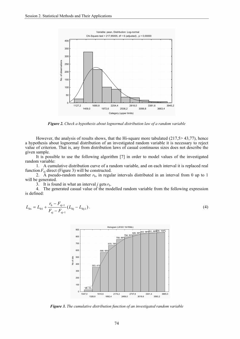
Let's construct the histogram of distribution (see Table 2, Figure 2). At selection of various
distribution laws by means of software package STATISTICA it has been established, that most precisely this sample will describe lognormal distribution law.
Table 2. Frequencies of the investigated random variable hit values in intervals
Intervals Quantity of hits Cumulative quantity of hits Percent of hits Cumulative percent of hit
<= 1328,80000 26 26 3,03030 3,0303
1610,60000 327 353 38,11189 41,1422 1892,40000 215 568 25,05828 66,2005 2174,20000 102 670 11,88811 78,0886 2456,00000 88 758 10,25641 88,3450 2737,80000 36 794 4,19580 92,5408 3019,60000 32 826 3,72960 96,2704 3301,40000 17 843 1,98135 98,2517 3583,20000 8 851 0,93240 99,1841 < Infinity 7 858 0,81585 100,0000
Session 2. Statistical Methods and Their Applications
74
Variable: реал, Distribution: Log-normalChi-Square test = 217,95005, df = 6 (adjusted) , p = 0,00000
1127,21409,0
1690,81972,6
2254,42536,2
2818,03099,8
3381,63663,4
3945,2
Category (upper limits)
0
50
100
150
200
250
300
350
400
No.
of o
bser
vatio
ns
Figure 2. Check a hypothesis about lognormal distribution law of a random variable
However, the analysis of results shows, that the Hi-square more tabulated (217,5> 43,77), hence
a hypothesis about lognormal distribution of an investigated random variable it is necessary to reject value of criterion. That is, any from distribution laws of casual continuous sizes does not describe the given sample.
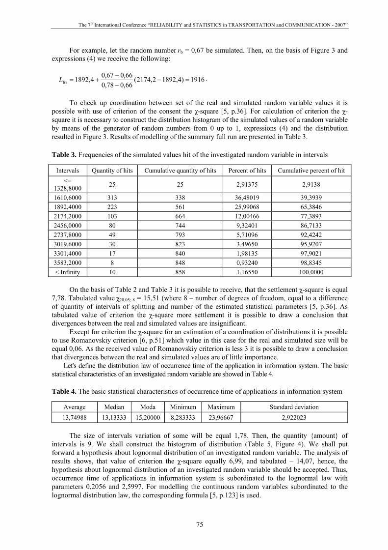
It is possible to use the following algorithm [7] in order to model values of the investigated random variable:
1. A cumulative distribution curve of a random variable, and on each interval it is replaced real function Fej direct (Figure 3) will be constructed.
2. A pseudo-random number rb, in regular intervals distributed in an interval from 0 up to 1 will be generated.
3. It is found in what an interval j gets rb. 4. The generated casual value of the modelled random variable from the following expression
is defined:
)( 1-frjfrj1еjеj
1еjbfr1frs LL
FFFr
LL −−
−+=
−
− . (4)
Histogram (LEGO 10v*858c)
26; 3%
353; 41%
568; 66%
670; 78%
758; 88%794; 93%
826; 96%843; 98%851; 99%858; 100%
1047,01328,8
1610,61892,4
2174,22456,0
2737,83019,6
3301,43583,2
3865,00
100
200
300
400
500
600
700
800
900
No
of o
bs
Figure 3. The cumulative distribution function of an investigated random variable
The 7th International Conference “RELIABILITY and STATISTICS in TRANSPORTATION and COMMUNICATION - 2007”
75
For example, let the random number rb = 0,67 be simulated. Then, on the basis of Figure 3 and expressions (4) we receive the following:
1916)4,18922,2174(66,078,066,067,04,1892frs =−
−−
+=L .
To check up coordination between set of the real and simulated random variable values it is
possible with use of criterion of the consent the χ-square [5, p.36]. For calculation of criterion the χ-square it is necessary to construct the distribution histogram of the simulated values of a random variable by means of the generator of random numbers from 0 up to 1, expressions (4) and the distribution resulted in Figure 3. Results of modelling of the summary full run are presented in Table 3.
Table 3. Frequencies of the simulated values hit of the investigated random variable in intervals
Intervals Quantity of hits Cumulative quantity of hits Percent of hits Cumulative percent of hit <=
1328,8000 25 25 2,91375 2,9138
1610,6000 313 338 36,48019 39,3939 1892,4000 223 561 25,99068 65,3846 2174,2000 103 664 12,00466 77,3893 2456,0000 80 744 9,32401 86,7133 2737,8000 49 793 5,71096 92,4242 3019,6000 30 823 3,49650 95,9207 3301,4000 17 840 1,98135 97,9021 3583,2000 8 848 0,93240 98,8345 < Infinity 10 858 1,16550 100,0000
On the basis of Table 2 and Table 3 it is possible to receive, that the settlement χ-square is equal
7,78. Tabulated value χ20,05; 8 = 15,51 (where 8 – number of degrees of freedom, equal to a difference of quantity of intervals of splitting and number of the estimated statistical parameters [5, p.36]. As tabulated value of criterion the χ-square more settlement it is possible to draw a conclusion that divergences between the real and simulated values are insignificant.
Except for criterion the χ-square for an estimation of a coordination of distributions it is possible to use Romanovskiy criterion [6, p.51] which value in this case for the real and simulated size will be equal 0,06. As the received value of Romanovskiy criterion is less 3 it is possible to draw a conclusion that divergences between the real and simulated values are of little importance.
Let's define the distribution law of occurrence time of the application in information system. The basic statistical characteristics of an investigated random variable are showed in Table 4. Table 4. The basic statistical characteristics of occurrence time of applications in information system
Average Median Moda Minimum Maximum Standard deviation 13,74988 13,13333 15,20000 8,283333 23,96667 2,922023
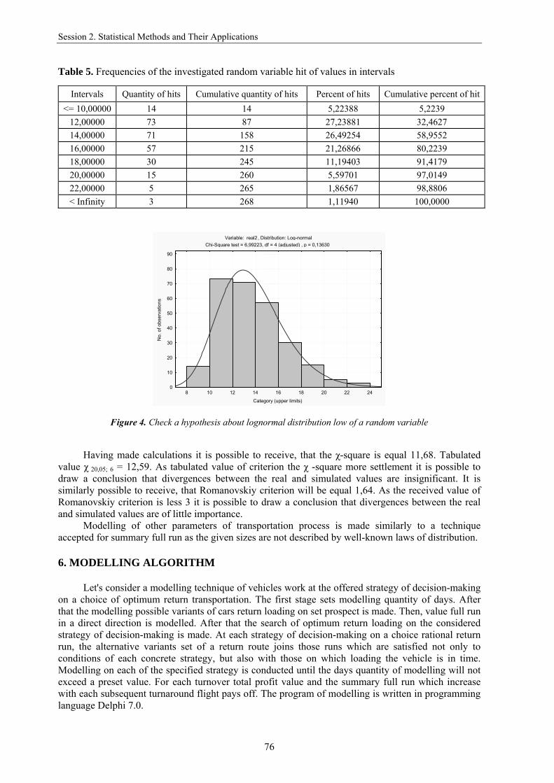
The size of intervals variation of some will be equal 1,78. Then, the quantity {amount} of intervals is 9. We shall construct the histogram of distribution (Table 5, Figure 4). We shall put forward a hypothesis about lognormal distribution of an investigated random variable. The analysis of results shows, that value of criterion the χ-square equally 6,99, and tabulated – 14,07, hence, the hypothesis about lognormal distribution of an investigated random variable should be accepted. Thus, occurrence time of applications in information system is subordinated to the lognormal law with parameters 0,2056 and 2,5997. For modelling the continuous random variables subordinated to the lognormal distribution law, the corresponding formula [5, p.123] is used.
Session 2. Statistical Methods and Their Applications
76
Table 5. Frequencies of the investigated random variable hit of values in intervals
Intervals Quantity of hits Cumulative quantity of hits Percent of hits Cumulative percent of hit <= 10,00000 14 14 5,22388 5,2239
12,00000 73 87 27,23881 32,4627 14,00000 71 158 26,49254 58,9552 16,00000 57 215 21,26866 80,2239 18,00000 30 245 11,19403 91,4179 20,00000 15 260 5,59701 97,0149 22,00000 5 265 1,86567 98,8806 < Infinity 3 268 1,11940 100,0000
Variable: real2, Distribution: Log-normalChi-Square test = 6,99223, df = 4 (adjusted) , p = 0,13630
8 10 12 14 16 18 20 22 24
Category (upper limits)
0
10
20
30
40
50
60
70
80
90
No.
of o
bser
vatio
ns
Figure 4. Check a hypothesis about lognormal distribution low of a random variable
Having made calculations it is possible to receive, that the χ-square is equal 11,68. Tabulated value χ 20,05; 6 = 12,59. As tabulated value of criterion the χ -square more settlement it is possible to draw a conclusion that divergences between the real and simulated values are insignificant. It is similarly possible to receive, that Romanovskiy criterion will be equal 1,64. As the received value of Romanovskiy criterion is less 3 it is possible to draw a conclusion that divergences between the real and simulated values are of little importance.
Modelling of other parameters of transportation process is made similarly to a technique accepted for summary full run as the given sizes are not described by well-known laws of distribution.
6. MODELLING ALGORITHM
Let's consider a modelling technique of vehicles work at the offered strategy of decision-making
on a choice of optimum return transportation. The first stage sets modelling quantity of days. After that the modelling possible variants of cars return loading on set prospect is made. Then, value full run in a direct direction is modelled. After that the search of optimum return loading on the considered strategy of decision-making is made. At each strategy of decision-making on a choice rational return run, the alternative variants set of a return route joins those runs which are satisfied not only to conditions of each concrete strategy, but also with those on which loading the vehicle is in time. Modelling on each of the specified strategy is conducted until the days quantity of modelling will not exceed a preset value. For each turnover total profit value and the summary full run which increase with each subsequent turnaround flight pays off. The program of modelling is written in programming language Delphi 7.0.

The 7th International Conference “RELIABILITY and STATISTICS in TRANSPORTATION and COMMUNICATION - 2007”
77
7. THE ANALYSIS OF THE MODELLING RESULTS Detailed results of automobile vehicles modelling work on the described algorithm and offered to
six strategy, by transportation cargoes on the international routes on prospect in half a year borrow volume equivalent to 2,5 thousand pages of format А4. Final results of calculations on each strategy of modelling are resulted in Table 6.
Table 6. Results of the vehicle work modelling on the international routes
Num
ber o
f stra
tegy
Max
imum
qua
ntity
of
hou
rs o
f ex
pect
atio
n of
oc
curr
ence
of t
he
appl
icat
ion,
h
Prof
it, B
YR
Sum
mar
y ru
n, k
m
Sum
mar
y at
one
o'
cloc
k, h
Prof
it on
1 k
m o
f ru
n, B
YR
/km
Prof
it at
one
o'cl
ock,
B
YR
/h
1 - 7038072 78116 4443,5 90,1 1583,9 2 - 7037577 78063 4443,5 90,2 1583,8
2 10327386 75806 4363,7 136,2 2366,7 5 9787644 78253 4390,1 125,1 2229,5 6 9831660 78097 4348,2 125,9 2261,1 8 10067834 78836 4393,1 127,7 2291,7
10 9540338 79267 4395,1 120,4 2170,7 12 10576096 81449 4353,5 129,8 2429,3 15 11183635 84718 4405,1 132,0 2538,8 20 10517640 74748 4386,2 140,7 2397,9
3
25 9808077 75105 4366,5 130,6 2246,2 2 10342863 76400 4362,6 135,4 2370,8 5 9463542 76819 4341,5 123,2 2179,8 6 10260885 78051 4391,1 131,5 2336,7 8 9737650 78038 4344,5 124,8 2241,4
10 9710435 78803 4324,5 123,2 2245,4 12 9072803 79388 4345,4 114,3 2087,9 15 8705019 79259 4371,5 109,8 1991,3 20 7832445 75924 4405,1 103,2 1778,0
4
25 6626094 74998 4338,3 88,4 1527,3 5 - 6998600 78063 4443,6 89,7 1575,0
Thus, if as the basic criterion of work to use total profit of an automobile carrier or a maximum
of economic feedback at one o'clock it is necessary to recommend to expect occurrence of the shipping cargoes request in the opposite direction no more than 15 hours. If as the basic criterion of work to use a maximum of an economic gain from one kilometre of run it is recommended to expect occurrence of the shipping cargo request in the opposite direction no more than 20 hours.
By development of practical recommendations on decision-making on a choice of rational behaviour strategy at a choice of optimum return transportation it is necessary to consider, that at modelling work of automobile means does not take into consideration time of "urgency" of the application located in information system. Under time of "urgency" of the application the period of time between occurrence of the application in information system and the moment of cargo offered acceptance to transportation by the given application should be considered. In the existing information systems time of "urgency" is not reflected. Therefore, at modelling work of an automobile vehicle it is supposed, that time of "urgency" of applications is not limited. That is, at decision-making on strategy 1-5 applications considered a circle it is limited to only admissible waiting time of occurrence of the application in information system. Of the set of possible applications received by such restrictions get out optimum by the accepted criterion. However, in practice while the carrier expects the expiration of
Session 2. Statistical Methods and Their Applications
78
an optimum waiting time of occurrence of the application, that cargo which transportation will give the maximal effect, can be already accepted to transportation by the competitor. Therefore, use in planning return transportations of strategy six which allows making a decision as quickly as possible on acceptance of a cargo to transportation on the basis of sufficient value of run operating ratio will be expedient. Modelling of automobile vehicle work an on the given strategy shows, that the total profit for half a year of work of the car will be equal 9884390 roubles. Thus the profit on one kilometre of run will make 133,4 BYR/km, and at one an hour – 2254,1 BYR/hour. Economic benefit in comparison with a variant of work on strategy 1 will make the order 5,6 million BYR a year from each vehicle. CONCLUSION
In the given work the actual problem of search and a choice optimum by return (passing return) loadings of an automobile vehicle working on the international routes is considered. The analysis of the literature has shown that there are short of the scientific techniques that allow solving the formulated problem. There has been developed six strategies of behaviour at decision-making on a choice of return transportation in this research for decision of the given problems. The lead statistical modelling automobile vehicles work on the international routes with size prospect equal half a year on each strategy and the detailed analysis of results of the given modelling has allowed to allocate optimum strategy. The essence of the given strategy consists that is considered serially, in the chronological order of receipt in information system all applications. For each considered variant the operating run ratio is defined and compared to a sufficient degree of use of cars run, certain of expression (3). To loading on the given strategy it is necessary to accept that cargo which transportation will give value of operating ratio of run not less than its sufficient size. Economic benefit of work on the given strategy in comparison with strategy put into practice now makes 2,3 thousand US dollars a year from each vehicle.
References
1. Azemsha, S.A., Sedyukevich, V.N. Criteria of Optimality for Routing the Main Automobile
Cargoes Transportations in View of Different Time Sending. In: Materials of the 2nd International Scientific and Technical Conference “Science – to Education, Manufacture, Economy”, vol. 1. Minsk: BNTU, 2004, pp. 279-281. (In Russian)
2. Azemsha, S.A. A Choice of the Operated Parameters o7f Efficiency Criterion of Main Cargo Automobile Transportations. In: Collection of Reports of the 8th Conference “Lithuania without Science – Lithuania without Future” of the Young Scientists of Lithuania. Vilnius: Techniques, 2005, pp. 306-311. (In Russian)
3. Azemsha, S.A. Strategy of Decision-Making at a Choice of Return Loading of the Automobile Vehicle Working on the International Routes. In: The Scientific and Technical Collection of Kharkov National Academy of Sciences “The Municipal Services of Cities”. Kiev: Techniques, 2006, pp. 307-314. (In Russian)
4. Azemsha, S.A. Definition of Dependence between Operated Parameters of Criterion of Efficiency of the Main Automobile Transportations by Motor Transport. In: Transport and Communication, 4. Riga: Institute of Transport and Communication, 2005, pp. 36-50. (In Russian)
5. Berezhnaya, E.V., Berezhnoy, V.I. Mathematical Methods of Economic Systems Modelling: studies manual, 2nd edition. М.: Finance and Statistics, 2005. 432 p. (In Russian)
6. Buldyk, G.M. Statistical Modelling and Forecasting: the textbook. Minsk: BUT Open Company "BIP-S", 2003. 399 p. (In Russian)
7. Kharin, Yu.S., Malyugin, V.I., Kirlitsa, V.P. etc. A Basis of Imitating and Statistical Modelling: studies manual. Minsk: Design PRO, 1997. 288 p. (In Russian)
8. Borovikov, V. STATISTICA. Art of the data analysis on a computer, for professionals. 2nd edition. St. Petersburg: Peter, 2003. 686 p. (In Russian)
9. Ginzburg, A.I. Statistics. St. Petersburg: Peter, 2003. 128 p. (In Russian)

The 7th International Conference “RELIABILITY and STATISTICS in TRANSPORTATION and COMMUNICATION - 2007”
79
ANALYSIS AND FORECAST OF THE URBAN PUBLIC TRANSPORT FLOW IN JURMALA CITY
Irina Yatskiv1, Alexander Medvedev1, Michael Savrasov1
Edgars Kreits2
1 Transport and Telecommunication Institute Lomonosova 1, Riga, LV-1019, Latvia
Phone: (+371)7100594. Fax: (+371)7100535. E-mail: [email protected] 2 Passenger Train, Ltd., Financial Department
Turgeneva 14, Riga, LV-1050, Latvia E-mail: [email protected]
This paper contains an analysis of urban public transport system in a small city in Latvia. The main task
of the analysis is to forecast the possible volume of public urban transport flow in Jurmala city on period 2008–2015. The situation in Jurmala is characterized practically as bimodal public urban transport – bus and suburban electric train, which function in parallel. Modelling the Jurmala public transport system is carried out by using PTV Vision software – VISUM Package.
Keywords: public urban transport, flow, forecast, regression models, exogenous variables, scenarios 1. INTRODUCTION
In obedience to strategy the «Sustainable transport» of World Bank [1] in area of development
of a transport sector is marked inseparable connection between the economic, social and ecological aspects of a steady transport policy. When planning the urban transportation facilities it is an obligatory task to forecast how much they will be used. There are many publications about forecasting for public transport demand for large cities, e.g. Madrid [2], Paris [3] etc. But often it is necessary to do it for small city or health-resort city such as Jurmala city is, for instance.
More useful technologies for forecasting passenger demands are presented in such monographs as J.Ortuzar&L.Willumsen [4] or Handbook of Transport Modelling [5]. In large cities with multimodal urban transport system the most important is to determine the demand for each alternative public transport mode. The theory of Discrete-Choice models developed by Ben Akiva, Lerman and others [6] is accepted in this case. In this disaggregate models it is necessary to take into account the next factors affecting the generation and attraction of trips: social status; life style and others characteristics of individual. Finally parameters of transport, such as expenses on moving, time of moving, punctuality, comfort, availability and quality of a transport infrastructure, have influence on the conduct of individual. To expose influence of numerous factors on passenger flow volume and take into account transport necessities of every separate traveller is a very complex practical problem and requires the well-developed system of Transport Survey, that, unfortunately, is absent in Jurmala city.
On the other hand the forecast can be fulfilled on the basis of the aggregated models, in which ethical and social norms should be considered. Such approach was used in Scenes (Scenarios for European Transport) models for public transport [7] and more useful for our case. So we need to establish the main integral factors which are the basis for populations’ demand on trip. 2. THE MAIN CHARACTERISTICS OF JURMALA TRANSPORT SYSTEM
The length of Jurmala city transport network is 364 km [8]. There are two modes of public
urban transport – “bus” mode and city train, which is the part of railway Riga – Ventspils. On 01.01.2006 the common amount of inhabitants equal 55602 [9]. For the last 10 years a tendency “permanent reduction of inhabitants” takes place in Jurmala city.
The park of cars, incorporated in Jurmala city, makes more than 25000 cars presently. The change of amount of the registered cars and busses is resulted on Figures 1-2 [10]. For the last six years the amount of private cars in Jurmala city is increased more than on 10000 units. The amount of busses is decreased for the last ten years, and presently puts together hardly more than 200 vehicles. As it is obvious, main influence on interests of public transport has the private transport of inhabitants (private cars). The motorization coefficient from data of 2006 makes 424 cars per 1000 persons in Jurmala city.

Session 2. Statistical Methods and Their Applications
80
Passenger transportations in city are provided on 10 routes of public transport, from which 6 routes of busses and 4 routes of mini busses. Apart from it a part of passenger transportation performs suburban electric trains. An information about distribution of passenger transportation between the busses’ routes from 2001 to 2006 [11] is showed on Fig. 3. The part of passengers, which are transported by the mini busses makes from 25% to 35% in different years. The part of passengers, which are transported on route 4 (claimed route), constitutes from 30% to 36% in different years.
Fig. 1. Amount of private cars in Jurmala city Fig. 2. Amount of buses in Jurmala city
Fig. 3. Distribution of the carried passengers between routes in Jurmala city
On the Fig. 4 information is showed about monthly transportations of passengers on all routes
for period from January 2001 till March 2007 [11]. It is obvious that the season component takes place in this time (seasonal lag equals 12). From the end of 2005 there the tendency on the decline of volume of transportations is observed.
Information of monthly transportation of passengers on the basic routes of busses for that period [11] is showed on Fig. 5. As it is obvious from the presented information, during a year on all routes the decline of volume of the carried passengers is considerable in the months of summer. It can account for vacations at secondary schools. From June to August an amount of the carried passengers goes down almost on 20-25%.
The scheme of passengers’ public routes in Jurmala city is presented on Fig. 6.
150000
200000
250000
300000
350000
01.01
.
05.01
.
09.01
.
01.02
.
05.02
.
09.02
.
01.03
.
05.03
.
09.03
.
01.04
.
05.04
.
09.04
.
01.05
.
05.05
.
09.05
.
01.06
.
05.06
.
09.06
.
01.07
.
Fig. 4. Monthly transportation of passengers (01. 2001-03.2007) in Jurmala city
Amounts of passengers
0
20000
40000
60000
80000
100000
120000
01.01
.
05.01
.
09.01
.
01.02
.
05.02
.
09.02
.
01.03
.
05.03
.
09.03
.
01.04
.
05.04
.
09.04
.
01.05
.
05.05
.
09.05
.
01.06
.
05.06
.
09.06
.
01.07
.
Summer time
Fig. 5. Monthly transportation of passengers route N 1; route N 2; route N 4; route N 6; route N 7; route N 8.
0%
20%
40%
60%
80%
100%
2001 2002 2003 2004 2005 2006
MiniBusN8N7N6N4N2N1
0
5000
10000
15000
20000
25000
1993 1994 1995 1996 1997 1998 1999 2000 2001 2002 2003 2004 2005 2006
050
100150200250300350400450500
1993 1994 1995 1996 1997 1998 1999 2000 2001 2002 2003 2004 2005 2006

The 7th International Conference “RELIABILITY and STATISTICS in TRANSPORTATION and COMMUNICATION - 2007”
81
Fig
. 6. T
he sc
hem
e of
pub
lic tr
ansp
ort r
oute
s in
Jurm
ala
city

Session 2. Statistical Methods and Their Applications
82
3. METHODOLOGY FOR THE FORECASTING OF THE PASSENGER TRANSPORTATION BY BUSES IN JURMALA CITY ON PERIOD 2008-2015
It is necessary to consider all levels of forecast: short-term (2008), medium-term (2008-2012)
and long-term (2012-2015) and accordingly the methods for forecast which are needed for each level. Application of method of extrapolation in short-term prognosis (for example, on the basis of
time series analysis) assumes that conformity to the law, operating in the past, will be saved in the forecast period, namely: a general progress of transportation trend must not suffer serious changes in the future. A medium-term prognosis is based on application of casual methods (regression analysis). A medium-term prognosis on the first two years can be corrected information about tendencies from a short-term prognosis. A long-term prognosis is based on application of casual methods and methods of expert estimations for the different scenarios of economy development (in this case – of Latvia and Jurmala city). The scheme of the methodology for forecasting is presented on a Fig. 7.
Factors, influencing on the production of common amount of movement, which must be using in regression analysis [7] are the following: profit, domain a car, structure of household, size of family, value of earth, closeness of residence, availability. The first 4 factors are examined almost always, 5 and 6 factors are used for the study of the zoned moving. The last one is used rarely, although is tried to include it always. Reason is in that if it was in equalization of regression, it will allow to estimate elasticity of generation of journeys in relation to the changes of a transport system.
Fig. 7. Methodology of forecast of passenger transportation by a public transport Because of the exogenous variables in a regression model often are unknown, therefore it is
necessary to forecast. And the prognosis can be on the basis of three scenarios, which differ at the level of assumptions. The scenarios of low and high growth between itself engulf the most credible range of future growth of trips: a base scenario is specified by the most probable value from this range. Master data for the construction of scenarios will be as follows:
• Information about the economy growing, determined as a prognosis of growth of GDP in the real prices in the real currency;
• Motorization level; • Strategic plan about the development of alternative modes of transport – networks of
railway (as alternative to the bus mode of transport in Jurmala city); • Carrying capacity of network; • Factors of load, suppositions about which must provide the linear change of traffic from
a present level to the future. They can be varied depending on an area and scenario; • Demographic changes (usually have unmeaning influence on the model of demand).
At the long-term prognosis the limitation of carrying capacity of the transport network is not taken into account. In this case a prognosis is built on the basis of model, taking into account six groups of factors:

The 7th International Conference “RELIABILITY and STATISTICS in TRANSPORTATION and COMMUNICATION - 2007”
83
As external factors come forward • characteristics of passengers – a group of factors, reflecting the amount of passengers and
their points of setting (without taking into account prices and economy growing). Many of these factors are included in the medium-term prognosis, but more expressly form group in the long-term prognosis;
• characteristics of economy – a group of factors, reflecting the economy growing, directly influencing on the size of demand for trips. Often these were incorporated in the factor of GDP growth factor;
• description of trip price – a group of factors, reflecting the cost of trip (ticket price trend, fuel price etc.).
As internal factors used • model of transport network, when new direct trips become able to force out trips with
transfers; • market structure which shows, what trips are created, to provide the forecast demand. In
particular, it includes assumption about the size of vehicles of transports, which for this purpose can be used;
• the model of carrying capacity of a transport network takes into account limitations, imposed the carrying capacity of some lines.
Fig. 8. Classification of factors, influencing on mobility of population Before forecasting travel for an urban area, it is necessary to define clearly the exact area to be
considered. This area is presented on Fig.6. Then for an analysis and forecast of passenger movements the Jurmala city is chosen and 9 areas are selected. The scopes of areas pass on the scopes of administrative boroughs, as it is shown in Table 1. Distribution of population between the selected areas is also showed in Table 1. As it is obvious from the resulting information, most concentration of population is on the area of Kauguri – more than 40% constantly live in this district. Table 1. Distribution of population in Jurmala city
Nr. Name of zones
Administrative area Number of inhabitants %
1. Lielupe Lielupe – Priedaine – Stirnukrogs – Buluciems – Varnukrogs 3438 6%
2. Bulduri Bulduri – Brazuciems 3644 7% 3. Dzintari Dzintari 2085 4% 4. Majori Majori 4082 7% 5. Dubulti Dubulti – Jaundubulti – Pumpuri – Druvciems 5291 10% 6. Melluzi Melluzi – Asari – Vaivari 4985 9% 7. Vaivari Vaivari – Sloka – Krastciems 6791 12% 8. Kauguri Kauguri – Kaugurciems – Bazciems – Brankciems 22658 41% 9. Kemeri Kemeri – Jaunkemeri – Kudra 2427 4% Total 55401 100

Session 2. Statistical Methods and Their Applications
84
These are not zones according classical theory of travel demand forecast, they need to be smaller. But zones are often grouped into larger units known as districts, that might contain 5 to 10 zones, and a city of a million must have about 100 districts. Districts often follow travel corridors, political jurisdictions, and natural boundaries such as rivers are. Unfortunately, statistics on passenger movement between zones on the routes of busses are absent. And for corresponding matrix (O-D matrix) the construction of the O-D matrix that consists from the information of passenger flow volume on a railway (the distribution between zones in %) was used. [12] 4. SCENARIOS OF PROGNOSIS AND EXOGENOUS PARAMETERS
DEVELOPMENT
For the forecast the three scenarios of economy development in Latvia are chosen: High, Base, Low. The Base scenario is most realistic and reflects economic trends and business existing today. The Low scenario is reflected by more pessimistic look on economy development in Latvia (disjoined and weak economy). The High scenario is yet more optimistic, than Base one (hasty economic growth).
In Table 2 the descriptions of three scenarios are resulting from the point of view of factors, influencing on functioning of public transport in Jurmala city. Unchanging is choosing a factor related to the demographic situation. In obedience to the report of Scenes [7] or World Population Prospect on 2010 and 2015 (UN, revision 2006) [13] a demographic situation in the Baltic countries scarcely will be sharply changed. The middle level of demographic situation is therefore chosen.
Table 2. The scenarios’ characteristics
Scenario High Base Low Passenger demand
Demographic situation Base
Economic factors
GDP Base +10% Base Base – 10%
Alternatives to the public transport
Private cars High Base Low
Rail Base
Also from the analysis of statistics of bus transportation the conclusion that tourism little influences on transportation in Jurmala city is made. Apart of it, the analysis of dependence between statistics of movement and a price of bus tickets is conducted, on the basis of which a decision about not including of this factor is also accepted in a model.
A railway and private car are the alternative modes of transport to transportation by buses. Both factors are taken into account in models. But if the factor ”private cars” included as the motorization coefficient (amounts of cars per 1000 inhabitants), the factor “railway” can have influence different appearance, depending on the plans of strategic development of railway and from the consequences of possible introduction of single electronic ticket. It is therefore decided to take into account it by introduction of correction coefficient on the final value of the forecast. Expert sets this coefficient. For more correct estimation of preference of different modes of transport it is necessary to make Transport Survey.
And, finally, the last factor, which can render substantial influencing on, is the changes of a transport network. However, substantial changes (such as new road and as a result introduction of new routes) in the near time are not foreseen. 5. PROGNOSIS OF EXOGENOUS FACTORS 5.1. Forecast of the Amount of Inhabitants in Jurmala City
Basic data for forecast of population in Jurmala is presented in a Table 3 [9]. The method of forecasting is divided on 2 stages: on the first stage – approximation from data of amount of population
The 7th International Conference “RELIABILITY and STATISTICS in TRANSPORTATION and COMMUNICATION - 2007”
85
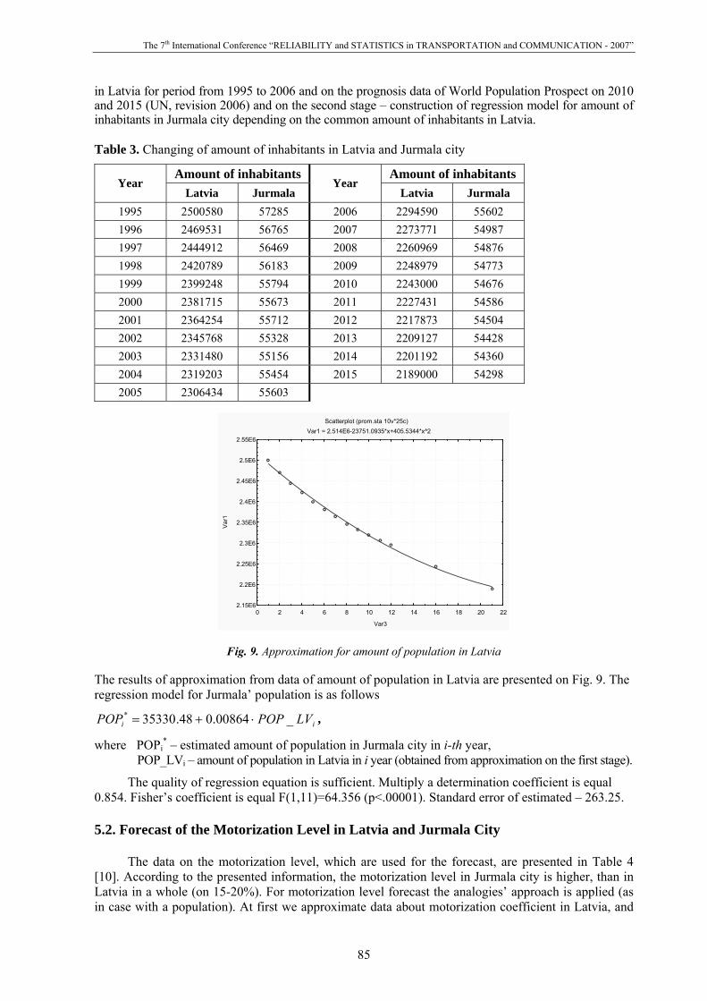
in Latvia for period from 1995 to 2006 and on the prognosis data of World Population Prospect on 2010 and 2015 (UN, revision 2006) and on the second stage – construction of regression model for amount of inhabitants in Jurmala city depending on the common amount of inhabitants in Latvia.
Table 3. Changing of amount of inhabitants in Latvia and Jurmala city
Amount of inhabitants Amount of inhabitants Year
Latvia Jurmala Year
Latvia Jurmala 1995 2500580 57285 2006 2294590 55602 1996 2469531 56765 2007 2273771 54987 1997 2444912 56469 2008 2260969 54876 1998 2420789 56183 2009 2248979 54773 1999 2399248 55794 2010 2243000 54676 2000 2381715 55673 2011 2227431 54586 2001 2364254 55712 2012 2217873 54504 2002 2345768 55328 2013 2209127 54428 2003 2331480 55156 2014 2201192 54360 2004 2319203 55454 2015 2189000 54298 2005 2306434 55603
Scatterplot (prom.sta 10v*25c)
Var1 = 2.514E6-23751.0935*x+405.5344*x^2
0 2 4 6 8 10 12 14 16 18 20 22
Var3
2.15E6
2.2E6
2.25E6
2.3E6
2.35E6
2.4E6
2.45E6
2.5E6
2.55E6
Var
1
Fig. 9. Approximation for amount of population in Latvia The results of approximation from data of amount of population in Latvia are presented on Fig. 9. The regression model for Jurmala’ population is as follows
ii LVPOPPOP _00864.048.35330* ⋅+= ,
where POPi* – estimated amount of population in Jurmala city in i-th year,
POP_LVi – amount of population in Latvia in i year (obtained from approximation on the first stage).
The quality of regression equation is sufficient. Multiply a determination coefficient is equal 0.854. Fisher’s coefficient is equal F(1,11)=64.356 (p<.00001). Standard error of estimated – 263.25. 5.2. Forecast of the Motorization Level in Latvia and Jurmala City
The data on the motorization level, which are used for the forecast, are presented in Table 4 [10]. According to the presented information, the motorization level in Jurmala city is higher, than in Latvia in a whole (on 15-20%). For motorization level forecast the analogies’ approach is applied (as in case with a population). At first we approximate data about motorization coefficient in Latvia, and
Session 2. Statistical Methods and Their Applications
86
then will build regression model for the motorization level in Jurmala city on the basis of the motorization level in Latvia.
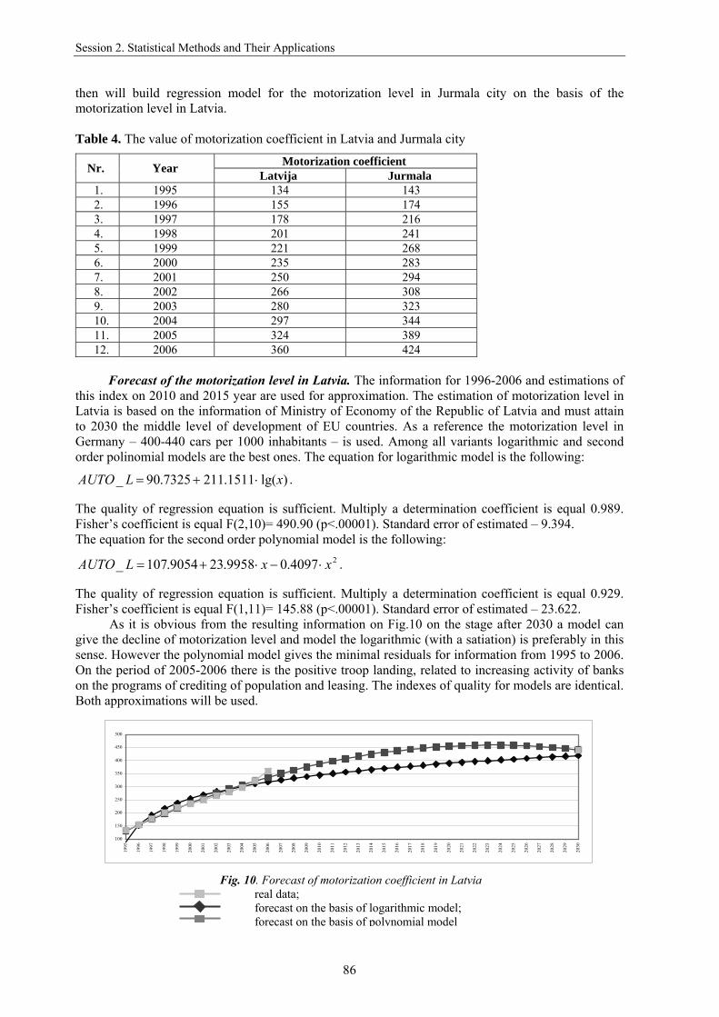
Table 4. The value of motorization coefficient in Latvia and Jurmala city
Motorization coefficient Nr. Year Latvija Jurmala 1. 1995 134 143 2. 1996 155 174 3. 1997 178 216 4. 1998 201 241 5. 1999 221 268 6. 2000 235 283 7. 2001 250 294 8. 2002 266 308 9. 2003 280 323 10. 2004 297 344 11. 2005 324 389 12. 2006 360 424
Forecast of the motorization level in Latvia. The information for 1996-2006 and estimations of
this index on 2010 and 2015 year are used for approximation. The estimation of motorization level in Latvia is based on the information of Ministry of Economy of the Republic of Latvia and must attain to 2030 the middle level of development of EU countries. As a reference the motorization level in Germany – 400-440 cars per 1000 inhabitants – is used. Among all variants logarithmic and second order polinomial models are the best ones. The equation for logarithmic model is the following:
)lg(1511.2117325.90_ xLAUTO ⋅+= .
The quality of regression equation is sufficient. Multiply a determination coefficient is equal 0.989. Fisher’s coefficient is equal F(2,10)= 490.90 (p<.00001). Standard error of estimated – 9.394. The equation for the second order polynomial model is the following:
24097.09958.239054.107_ xxLAUTO ⋅−⋅+= .
The quality of regression equation is sufficient. Multiply a determination coefficient is equal 0.929. Fisher’s coefficient is equal F(1,11)= 145.88 (p<.00001). Standard error of estimated – 23.622.
As it is obvious from the resulting information on Fig.10 on the stage after 2030 a model can give the decline of motorization level and model the logarithmic (with a satiation) is preferably in this sense. However the polynomial model gives the minimal residuals for information from 1995 to 2006. On the period of 2005-2006 there is the positive troop landing, related to increasing activity of banks on the programs of crediting of population and leasing. The indexes of quality for models are identical. Both approximations will be used.
100
150
200
250
300
350
400
450
500
1995
1996
1997
1998
1999
2000
2001
2002
2003
2004
2005
2006
2007
2008
2009
2010
2011
2012
2013
2014
2015
2016
2017
2018
2019
2020
2021
2022
2023
2024
2025
2026
2027
2028
2029
2030
Fig. 10. Forecast of motorization coefficient in Latvia real data; forecast on the basis of logarithmic model; forecast on the basis of polynomial model

The 7th International Conference “RELIABILITY and STATISTICS in TRANSPORTATION and COMMUNICATION - 2007”
87
Forecast the motorization level in Jurmala city. The regression model for the motorization level in Jurmala city on the motorization level in Latvia using data of period 1995-2006 (see Fig. 11) is built. The results of calculations are presented in Table 5. The quality of regression equation is sufficient.
Scatterplot (prom.sta 10v*25c)Auto_J = -7.9649+1.2072*x
120 140 160 180 200 220 240 260 280 300 320 340 360 380
Auto_L
100
150
200
250
300
350
400
450
Aut
o_J
Auto_L:Auto_J: r2 = 0.9926; r = 0.9963, p = 0.0000; y = -7.9649215 + 1.20716156*x
Fig. 11. Regression equation for motorization level in Jurmala city
Table 5. Estimated values of motorization levels in Latvia and in Jurmala city
Logarithmic model Polinomial model Nr. Year Latvija Jurmala Latvija Jurmala 1. 2008 333 394 364 431 2. 2009 339 401 376 446 3. 2010 345 408 387 459 4. 2011 351 415 397 472 5. 2012 356 422 407 483 6. 2013 361 428 416 494 7. 2014 365 433 424 504 8. 2015 370 439 431 513
As the base for motorization level (Base scenario) maximum of two approximations, as the level for the Low scenario – minimum of two approximations are used. And as the level for the High scenario is the level for the Base scenario increased on 10%. 5.3. Forecast of Amount of Private Cars in Jurmala City The estimated value of amount of cars in Jurmaly city is calculated
iii POPMOTAUTO ⋅= ,
where POPi – the amount of population in Jurmala city in the i-th moment of time MOTi – a motorization level (amount of cars per 1000 inhabitants)
The results of calculations are presented in Table 6. 5.4. Forecast of Gross Domestic Product (GDP)
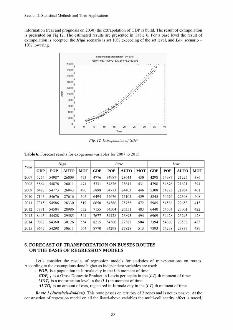
For forecasting information of the Latvian Statistical Bureau on the volumes of GDP is used [9]. On a prognosis to 2030 Latvia must attain a middle level on ЕС (as one of variants – current level of GDP of Germany). On 2005 the level of GDP of Germany made 18985 Ls per person. Using
Session 2. Statistical Methods and Their Applications
88
information (real and prognosis on 2030) the extrapolation of GDP is build. The result of extrapolation is presented on Fig.12. The estimated results are presented in Table 6. For a base level the result of extrapolation is accepted, the High scenario is set 10% exceeding of the set level, and Low scenario – 10% lowering.
Fig. 12. Extrapolation of GDP Table 6. Forecast results for exogenous variables for 2007 to 2015
High Base Low Year
GDP POP AUTO MOT GDP POP AUTO MOT GDP POP AUTO MOT
2007 5254 54987 26009 473 4776 54987 23644 430 4298 54987 21225 386 2008 5864 54876 26011 474 5331 54876 23647 431 4798 54876 21621 394 2009 6487 54773 26843 490 5898 54773 24403 446 5308 54773 21964 401 2010 7143 54676 27616 505 6494 54676 25105 459 5845 54676 22308 408 2011 7315 54586 28330 519 6650 54586 25755 472 5985 54586 22653 415 2012 7871 54504 28986 532 7155 54504 26351 483 6440 54504 23001 422 2013 8445 54428 29585 544 7677 54428 26895 494 6909 54428 23295 428 2014 9037 54360 30126 554 8215 54360 27387 504 7394 54360 23538 433 2015 9647 54298 30611 564 8770 54298 27828 513 7893 54298 23837 439
6. FORECAST OF TRANSPORTATION ON BUSSES ROUTES
ON THE BASIS OF REGRESSION MODELS
Let’s consider the results of regression models for statistics of transportations on routes. According to the assumptions done higher as independent variables are used:
- POPi is a population in Jurmala city in the i-th moment of time; - GDPi -1 is a Gross Domestic Product in Latvia per capita in the (i-1)-th moment of time; - MOTi is a motorization level in the (i-1)-th moment of time; - AUTOi is an amount of cars, registered in Jurmala city in the (i-1)-th moment of time.
Route 1 (Jūraslīcis-Bulduri). This route passes on territory of 2 zones and is not extensive. At the construction of regression model on all the listed-above variables the multi-collinearity effect is traced,
Scatterplot (Spreadsheet1 9v*37c)GDP = 587.1909+216.4727*x+8.2462*x^2
-5 0 5 10 15 20 25 30 35 40
Time
0
2000
4000
6000
8000
10000
12000
14000
16000
18000
20000G
DP
The 7th International Conference “RELIABILITY and STATISTICS in TRANSPORTATION and COMMUNICATION - 2007”
89
that is confirmed a presence by meaningful pair correlation between all factors (like for other routes). The best model for the estimation of amount of passengers on this route is the following:
( )1* _ln58.5060876.2486.8476101_ −⋅−⋅+−= iii LGDPPOPPass . (1)
Route 2 (Slokas railway station-Kauguri (Raiņa street)). This route is similar to the previous one, passes through 2 zones, and is not extensive too. The best model for the estimation of amount of passengers on the route 2 has the same form as for the previous route:
( )1* _ln15.721564.5664.23509192_ −⋅−⋅+−= iii LGDPPOPPass . (2)
Route 4 (Bulduri-Kauguri). This route is one of the most extensive and passes 7 zones of Jurmala city. A route also leads on volume transportation. The best model for the estimation of amount of passengers on the route 4 has the following form:
( )1* _ln62.29489256.6143.250724_ −⋅−⋅+= iii LGDPPOPPass . (3)
Route 6 (Slokas bus terminal-Ķemeri). A route passes through 3 zones. The best model for estimation the amount of passengers on a route 6 has the form of model as for the previous route:
( )1* _ln66.15467212.728.12031386_ −⋅−⋅+= iii LGDPPOPPass . (4)
In Table 7 values of quality criteria for models of transportation volumes on the busses routes are showed.
Table 7. Quality indices for regression models
Nr. of route 1. 2. 4. 6. Variables POP,GDP POP,GDP POP,GDP POP,GDP
Multiple R 0.9114 0.9291 0.9557 0.9794 Multiple R2 0.8307 0.8632 0.9134 0.9592 Adjusted R2 0.7930 0.8329 0.8942 0.9501
F(2,9) 22.07 28.41 47.47 105.73 p-value 0.0003 0.0001 0. 00002 0.000001
Std.Err.ofEstimate 18520 28789.83 57327.3 17035.73 Durbin-Watson 1.43 1.13 1.77 1.97
Error, % 12.52 11.59 4.9 4.13
Route 7 (Priedaine-Dubultu railway overpass). A route falls into category extensive and affects 5 areas. Unfortunately, on this route it is not succeeded to build a high-quality model for the estimation of amount of passengers on a route.
Route 8 (RIMI-Slokas bus terminal). A route is affected by 7 areas and also falls into a category of extensive one. Unfortunately, on this route it is not also succeeded to build a high-quality model for the estimation of amount of passengers on the route. It is possible to assume that development of situation on these routes is alike the situation on the other routes. In order to find the most similar routes by 7 and 8, a cluster analysis for dividing of routes into homogeneous groups is applied. As characteristics of routes, let’s use length of route, amount of zones, which it passes through, time of motion on a route (in sec.) and amount of the carried passengers for 2006. The values of these indices for the examined routes of busses are showed in Table 8.
For classification the data is standardized and the hierarchical and iterative methods of cluster analysis are applied. On Fig. 13 the classification tree is revealed. It is possible to suppose the presence of three classes of routes: the 1st class contains 1 and 2 routes, the 2nd class – 7 and 6, and the 3rd class – the most extensive routes and the routes 4 and 8 affect plenty of areas. Due to this classification, principle of analogy for forecast of the future situation on routes 7 and 8 is applied, namely: for route 7 –the tendency similar to route 6 is chosen, and for route 8 – tendency of the route 4.

Session 2. Statistical Methods and Their Applications
90
Tree Diagram for 6 CasesWard`s method
City-block (Manhattan) distances
M8 M4 M7 M6 M2 M10
2
4
6
8
10
12
Link
age
Dis
tanc
e
Table 8. Descriptions of the busses routes
Fig. 13. Classification tree for busses routes
7. SHORT-TERM FORECAST ON YEAR 2008
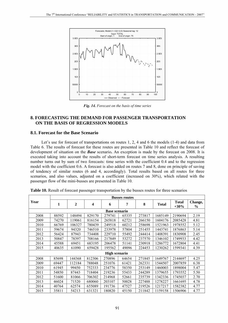
Based on monthly information on transportations, forecasts for total volume and for volume on separate routes (only busses) are built on the base of time series analysis. The models are built by the Box-Jenkins method [14]. Based on the research of nature of this time series (conducted on the stage of authentication of model of ARIMA) the seasonal model of ARIMA is chosen with seasonal lag equal 12. Models differ to the order of autoregression (1 or 2). The models of type ARIMA(1,1,0)(1,0,0)12 or ARIMA(1,1,0)(2,0,0)12 turned out as a result of selection. Within the framework of model of ARIMA information is transformed by differentiation un-seasonally (with lag equal 1) and seasonally (with lag equal 12). Results for 7 models are presented in Table 9 and on Fig. 7.
Table 9. Estimated results of transportations on busses routes and in total
on the basis of time series analysis
Nr. of busses route Date 1 2 4 6 7 8
Total
JAN_08 8232 13732 66961 23761 5292 23411 177948
FEB_08 7784 13745 63692 21427 4870 22210 174899
MAR_08 8232 15365 65070 22578 5353 24228 188637
APR_08 8455 15611 67104 23796 5451 24116 187887
MAI_08 8504 14776 68773 24329 5034 25103 187958
JUN_08 7569 12466 67984 22081 4462 22665 183484
JUL_08 6740 11436 53547 18467 3602 18573 166437
AUG_08 6659 11607 54251 18122 3832 18624 165188
SEP_08 9145 16336 71520 25384 5845 29153 186541
OKT_08 9055 16093 71930 25078 5762 25416 184949
NOV_08 8801 15522 70320 24379 5546 24943 177434
DEC_08 8700 15282 71320 24098 4891 23060 174084
Because technology of forecast by the models of time series is applicable only for a short-term,
it is obviously traced on the forecast – it saves the tendencies of the last two years (see Fig. 14). In order to take into account the change of external terms (standard of living of population and etc.) it is necessary forecast on the models of time series on 2008 to correct on the basis of forecast on regression models.
Route Length Time Amount of zones
Amount of carried
passengers 1 4.48 528 2 98209 2 2.84 84 2 172296 4 16.35 1171 7 830469 6 13.897 947 3 272228 7 10.62 755 5 68057 8 21.793 1550 7 281705
The 7th International Conference “RELIABILITY and STATISTICS in TRANSPORTATION and COMMUNICATION - 2007”
91
Fig. 14. Forecast on the basis of time series 8. FORECASTING THE DEMAND FOR PASSENGER TRANSPORTATION
ON THE BASIS OF REGRESSION MODELS 8.1. Forecast for the Base Scenario
Let’s use for forecast of transportations on routes 1, 2, 4 and 6 the models (1-4) and data from Table 6. The results of forecast for these routes are presented in Table 10 and reflect the forecast of development of situation on the Base scenario. An exception is made by the forecast on 2008. It is executed taking into account the results of short-term forecast on time series analysis. A resulting number turns out by sum of two forecasts: time series with the coefficient 0.4 and to the regression model with the coefficient 0.6. A forecast is also added on routes 7 and 8, done on principle of saving of tendency of similar routes (6 and 4, accordingly). Total results based on all routes for three scenarios, and also values, adjusted on a coefficient (increased on 30%), which related with the passenger flow of the mini-busses are presented in Table 10. Table 10. Result of forecast passenger transportation by the busses routes for three scenarios
Busses routes Year 1 2 4 6 7 8 Total Total
+30% Change,
% Base scenario
2008 88592 148494 829170 279741 65335 273817 1685149 2190694 2.19 2009 74270 119061 816154 265818 62721 266150 1604176 2085428 4.81 2010 66769 106327 780439 249518 60212 258698 1521963 1978552 5.12 2011 59674 94320 746510 233978 57804 251455 1443741 1876863 5.14 2012 56424 87943 734408 229710 55492 244414 1408391 1830908 2.45 2013 50847 78397 708166 217849 53272 237570 1346102 1749933 4.42 2014 45588 69451 683195 206478 51141 230918 1286772 1672804 4.41 2015 40635 61090 659428 195562 49096 224453 1230262 1599341 4.39
High scenario 2008 85698 144368 812306 270896 64654 271845 1649767 2144697 4.25 2009 69447 112184 788048 251076 61421 262331 1544507 2007859 6.38 2010 61945 99450 752333 234776 58350 253149 1460003 1898004 5.47 2011 54850 87443 718404 219236 55433 244289 1379655 1793552 5.50 2012 51600 81066 706302 214968 52661 235739 1342336 1745037 2.70 2013 46024 71520 680060 203107 50028 227488 1278227 1661695 4.78 2014 40764 62574 655089 191736 47527 219526 1217217 1582382 4.77 2015 35811 54213 631321 180820 45150 211842 1159158 1506906 4.77
Forecasts; Model:(1,1,0)(1,0,0) Seasonal lag: 12Input: TOTAL
Start of origin: 1 End of origin: 75
0 10 20 30 40 50 60 70 80 90 100
Observed Forecast
0
50000
1E5
1.5E5
2E5
2.5E5
3E5
3.5E5
0
50000
1E5
1.5E5
2E5
2.5E5
3E5
3.5E5
Session 2. Statistical Methods and Their Applications
92
Busses routes Year 1 2 4 6 7 8 Total Total
+30% Change,
% Low scenario
2008 91791 153056 847812 289518 66015 274662 1722855 2239712 0.01 2009 79602 126664 847224 282115 64035 267796 1667435 2167666 3.22 2010 72101 113930 811509 265814 62114 261101 1586568 2062539 4.85 2011 65006 101923 777580 250275 60250 254573 1509607 1962489 4.85 2012 61756 95546 765478 246006 58443 248209 1475438 1918070 2.26 2013 56179 85999 739237 234146 56690 242004 1414254 1838530 4.15 2014 50920 77054 714265 222775 54989 235954 1355956 1762743 4.12 2015 45967 68692 690498 211858 53339 230055 1300409 1690532 4.10
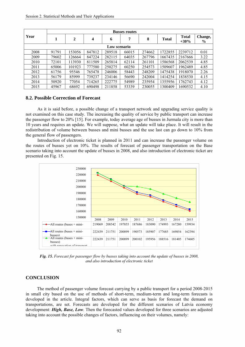
8.2. Possible Correction of Forecast
As it is said before, a possible change of a transport network and upgrading service quality is not examined on this case study. The increasing the quality of service by public transport can increase the passenger flow to 20% [15]. For example, today average age of busses in Jurmala city is more than 10 years and requires an update. We will suppose, what an update will take place. It will result in the redistribution of volume between busses and mini busses and the use last can go down to 10% from the general flow of passengers.
Introduction of electronic ticket is planned in 2011 and can increase the passenger volume on the routes of busses yet on 10%. The results of forecast of passenger transportation on the Base scenario taking into account the update of busses in 2008, and also introduction of electronic ticket are presented on Fig. 15.
Fig. 15. Forecast for passenger flow by busses taking into account the update of busses in 2008,
and also introduction of electronic ticket CONCLUSION
The method of passenger volume forecast carrying by a public transport for a period 2008-2015 in small city based on the use of methods of short-term, medium-term and long-term forecasts is developed in the article. Integral factors, which can serve as basis for forecast the demand on transportations, are set. Forecasts are developed for the different scenarios of Latvia economy development: High, Base, Low. Then the forecasted values developed for three scenarios are adjusted taking into account the possible changes of factors, influencing on their volumes, namely:
150000
160000
170000
180000
190000
200000
210000
220000
230000
All routes (buses + mini- 219069 208542 197855 187686 183090 174993 167280 159934
222439 211751 200899 190573 185907 177685 169854 162394
222439 211751 200899 200102 195956 188516 181405 174605
2008 2009 2010 2011 2012 2013 2014 2015
All routes (buses + mini-busses) All routes (buses + mini-busses) with renovation of transport

The 7th International Conference “RELIABILITY and STATISTICS in TRANSPORTATION and COMMUNICATION - 2007”
93
- multiplying the quality level of transportations (at the result of update of busses park); - introduction of single electronic ticket on a public urban transport in Jurmala city.
Analysis of situation with passenger transportations by busses in Jurmala city, conducted in the article, allowed formulating the following conclusions:
• At any scenario of Latvia economy development the steady decline of volumes of carrying passengers by public transport in Jurmala city will take place.
• Diminishing of volumes of carrying passengers is conditioned by the following factors: the tendency for Jurmala city to the decline of number of inhabitants which are
working in city; the growth of GDP and to the special role of Jurmala city as the so-called «sleeping
area of Riga» for people with income above the average; increasing the motorization level of population in Latvia and intensity of the use of
individual transport; presence of railway, as alternative to bus transportation; low level of quality of service, related foremost to the out-of-date bus park.
References 1. World Bank.1996.Sustainable Transport: Priorities or Policy Reform. A World Bank Policy
Paper.Washington, D.C. 2. García-Ferrer, A., Juan, A., Poncela, P., Bujosa, M. Monthly Forecasts of Integrated Public
Transport Systems: The Case of the Madrid Metropolitan Area, Journal of Transportation and Statistics, Vol.7, No1.
3. Fox, J., Daly, A., Gunn, H. Review of RAND Europe’s Transport Demand Model Systems. RAND, 2003. 92 p.
4. Transport modelling, 3rd edition / Ed. by Juan de Dios Ortuzar, Luis G.Willumsen. NY: Wiley, 2005. 499 p.
5. Handbook of Transport Modelling /Ed. by David A. Hensher, Kennet J. Buton. NY: Pergamon, 2000. 666 p.
6. Ben-Akiva, M., Lerman, S.R. Discrete Choice Analysis: theory and application to travel demand. Cambridge, Ma: MIT Press, 1985.
7. Project „SCENES”, Deliverable D3a, D3b, 2000. 8. Jurmala Development Plan, 2007. 9. The Internet site – www.csb.gov.lv (Latvian Central Statistical Bureau) 10. The Internet site – www.csdd.lv (Ceļu Satiksmes Drošības Direkcija) 11. Data by the company „ International and Local Passenger Transportation by Busses and Freight
Transportation” Ltd. (In Latvian) 12. Data of the Joint Stock Company “Passengers’ Train”. (In Latvian) 13. The Internet site – http://esa.un.org/unpp/ (World Population Prospects: The 2006 revision
Population Database). 14. Chatfield, C. The Analysis of Time Series, 4th edition. Chapman&Hall, 1995. 241 p. 15. The Up-to-Date Tram’s Project: the first phase account. Riga: SYSTRA, 2002. (In Latvian)

Session 2. Statistical Methods and Their Applications
94
APPLICATION OF MESOSCOPIC MODELLING FOR QUEUING SYSTEMS RESEARCH
Michael Savrasov, Yury Toluyew
Transport and Telecommunication Institute
Lomonosova 1, Riga, LV-1019, Latvia Phone: (+371)29654003. E-mail: [email protected]
Simulation can be used to solve wide range of practical problems. Usually simulation on microscopic level is used to solve practical problems. But such approach of simulation has its own disadvantages. Full system functionality algorithm must be created; also all objects involved must be described in details. This lead us to the problem of wasting a lot of time on creating such complex models, holding experiments with them, collecting and process a lot of data. Simulation on mesoscopic level usually does not have such problems, because of aggregating of homogeneous objects. Also results of simulation on mesoscopic level can be introduced as graphs of processes, which are very useful on practice. The concept of simulation on mesoscopic level specifies the development of principally new class of models. For which the task of testing such class of model using numerical examples is actual. In this article are described a results of such testing, comparing the output of mesoscopic models of queuing system and result of simulation on microscopic level with the GPSS World.
Keywords: mesoscopic simulation, queuing systems 1. INTRODUCTION
Simulation can be used to solve wide range of practical problems. A lot of such problems operate with flows: car flows, cargo flows, pedestrian’s flows etc. Historically such problems can be solved using simulation on micro and macro level. Both of these simulation types can be used. On the one hand there is macroscopic simulation used to model relatively large number of units that are distributed in abstract space. Analogous to gases and liquids, physical laws and therefore differential equations can describe movement of units in space. Using this method of simulation sometimes it is very useful creating complex forecasts, but we should understand that result is calculated from aggregated data and therefore result can not be very exact. In microscopic simulation on the other hand every moving object represents exactly one unit. A lot of options of unit can be taken in to account for calculations and final result will be more confidence. But such approach of simulation has its own disadvantages. Full system functionality algorithm must be created, also all objects involved, must be described in details. This lead us to the problem of wasting a lot of time on creating such models, holding experiments with them, collecting and process a lot of data. Both micro and macro simulation have their disadvantages, that is why simulation on mesoscopic level can be used.
The term mesoscopic is interpreted differently but nowhere as a “third type” of modelling distinguished from both macroscopic modelling based on differential equations and microscopic discrete process simulation. The philosophy behind this approach can be described with the phrase “discrete time/ continuous quantity” [1]. The representation of individual flow objects that reproduce persons, job orders, goods etc. is dispensed with. Instead only the members are employed, which are used in the model to represent respective quantities of objects or materials and can be modified with mathematical formula in every step of the discrete simulation time. This type of mesoscopic modelling and simulation is a method to quickly complete planning tasks in production, logistics systems etc. Also results of simulation on mesoscopic level can be introduced as graphs of processes, which are very useful on practice. The concept of simulation on mesoscopic level specifies the development of principally new class of models. That is why the task of testing such class of models is actual using numerical examples. As the testing objects queuing systems are taken.
2. MESOSCOPIC MODEL
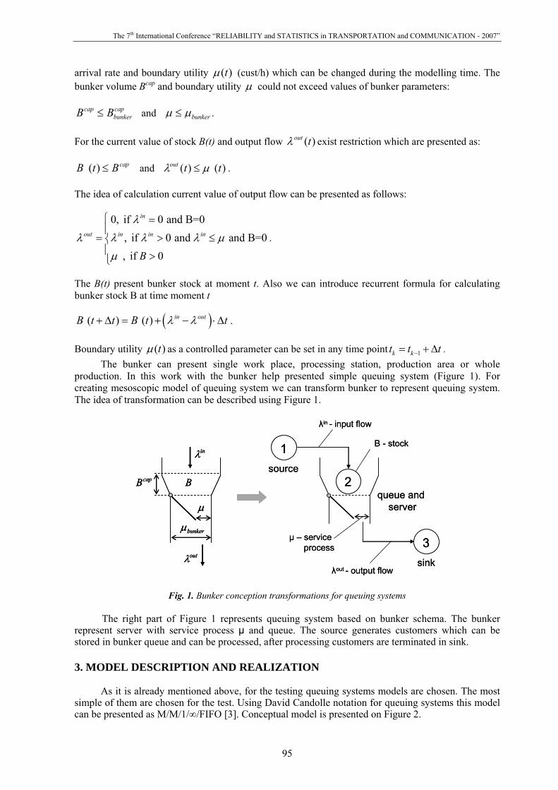
Formally mesoscopic models can be represented as bunker. Left side of Figure 1 presents classical conceptual schema of bunker [2]. The bunker has input flow of customers which can be described by arrival rate – ( )in tλ (cust/h). Inter arrival rate of output flow ( )out tλ (cust/h) depends on
The 7th International Conference “RELIABILITY and STATISTICS in TRANSPORTATION and COMMUNICATION - 2007”
95
arrival rate and boundary utility ( )tμ (cust/h) which can be changed during the modelling time. The bunker volume Bcap and boundary utility μ could not exceed values of bunker parameters:
capbunker
cap BB ≤ and bunkerμμ ≤ .
For the current value of stock B(t) and output flow ( )out tλ exist restriction which are presented as:
capBtB ≤)( and )()( ttout μλ ≤ . The idea of calculation current value of output flow can be presented as follows:
0, if 0 and B=0, if 0 and and B=0, if 0
in
out in in in
B
λ
λ λ λ λ μ
μ
⎧ =⎪
= > ≤⎨⎪ >⎩
.
The B(t) present bunker stock at moment t. Also we can introduce recurrent formula for calculating bunker stock B at time moment t
( )( ) ( ) in outB t t B t tλ λ+ Δ = + − ⋅Δ . Boundary utility ( )tμ as a controlled parameter can be set in any time point 1k kt t t−= + Δ .
The bunker can present single work place, processing station, production area or whole production. In this work with the bunker help presented simple queuing system (Figure 1). For creating mesoscopic model of queuing system we can transform bunker to represent queuing system. The idea of transformation can be described using Figure 1.
Fig. 1. Bunker conception transformations for queuing systems
The right part of Figure 1 represents queuing system based on bunker schema. The bunker represent server with service process μ and queue. The source generates customers which can be stored in bunker queue and can be processed, after processing customers are terminated in sink.
3. MODEL DESCRIPTION AND REALIZATION
As it is already mentioned above, for the testing queuing systems models are chosen. The most simple of them are chosen for the test. Using David Candolle notation for queuing systems this model can be presented as M/M/1/∞/FIFO [3]. Conceptual model is presented on Figure 2.
1source
λin - input flow
λout - output flow
μ – serviceprocess
B - stock
3sink
queue andserver
2
outλ
inλ
μ
BcapB
bunkerμ
1source
λin - input flow
λout - output flow
μ – serviceprocess
B - stock
3sink
queue andserver
2
outλ
inλ
μ
BcapB
bunkerμ
outλ
inλ
μ
BcapB
bunkerμ

Session 2. Statistical Methods and Their Applications
96
Fig. 2. Conceptual model of tested queuing system
As it can be seen on Figure input flow is distributed by exponential law with arrival rate λ=50. Server can process customers with exponential law with parameter μ(t). Service process presented as function:
30, 0 445, 4 840, 8 12
( )50, 12 1640, 16 2080, 20 24
ttt
tttt
μ
< ≤⎧⎪ < ≤⎪⎪ < ≤
= ⎨ < ≤⎪⎪ < ≤⎪
< ≤⎩
Amount of slots on server is 1, queue before server is not limited and queue type is FIFO. The simulation time is 24 time units (24 hours).
Using conceptual model it is easy to create GPSS model [4] which represent tested system. The GPSS code is presented on Figure 3. The code does not include service code which is used for experiment carrying.
Fig. 3. GPSS code of first tested model The mesoscopic model is created in Microsoft Excel using integrated components and macroses are written on Visual Basic for Application language. The results of modelling are presented using graphs and numerical data. 4. THE FIRST EXPERIMENT
The main goal of the first experiment is to compare output parameters of simulation model on microlevel with output parameters from mesoscopic model. As the output parameters we consider the following: average queue length, max queue length and queue length on simulation end. As the input flow rate for mesoscopic model empirical values of arrival rate from GPSS are used. That is done
OB FUNCTION C1,D6 4,30/8,45/12,40/16,50/20,40/24,80 GENERATE (EXPONENTIAL(1,0,1/50)) QUEUE rinda SEIZE srv DEPART rinda ADVANCE (EXPONENTIAL(1,0,(1/FN$OB))) RELEASE srv TERMINATE GENERATE 24 TERMINATE 1 START 1

The 7th International Conference “RELIABILITY and STATISTICS in TRANSPORTATION and COMMUNICATION - 2007”
97
because normally the input flow is a well-known process. But, of course, if empirical values of input flow are not known, the theoretical arrival rate can be used. In all experiments value of Δt is 1 hour.
Fig. 4. Input flow, service process, output flow for first experiment As the service rate theoretical values determined by function μ(t) are used. The input, output flow and service process is presented graphically on Figure 4.
The main goal of experiment is to compare different metrics of queue for both simulation approaches. On Figure 5 is presented a graph, which introduces queue length fixed every hour for both models. The results for micro-simulation models are average of 10 runs with different seeds for random numbers generators.
Queue length
050
100150200250
0 1 2 3 4 5 6 7 8 9 10 11 12 13 14 15 16 17 18 19 20 21 22 23 24
t (hours)
cust
.
Mesoscopic modelMicroscopic model
Fig. 5. Queue length changing process
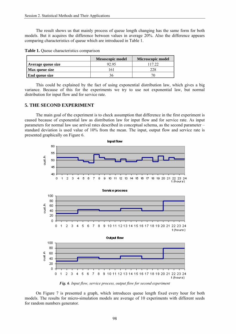
Session 2. Statistical Methods and Their Applications
98
The result shows us that mainly process of queue length changing has the same form for both models. But it acquires the difference between values in average 20%. Also the difference appears comparing characteristics of queue which are introduced in Table 1.
Table 1. Queue characteristics comparison
Mesoscopic model Microscopic model Average queue size 92.95 117.22 Max queue size 161 228 End queue size 36 70
This could be explained by the fact of using exponential distribution law, which gives a big
variance. Because of this for the experiments we try to use not exponential law, but normal distribution for input flow and for service rate. 5. THE SECOND EXPERIMENT
The main goal of the experiment is to check assumption that difference in the first experiment is caused because of exponential law as distribution law for input flow and for service rate. As input parameters for normal law use arrival rates described in conceptual schema, as the second parameter – standard deviation is used value of 10% from the mean. The input, output flow and service rate is presented graphically on Figure 6.
Fig. 6. Input flow, service process, output flow for second experiment
On Figure 7 is presented a graph, which introduces queue length fixed every hour for both
models. The results for micro-simulation models are average of 10 experiments with different seeds for random numbers generator.

The 7th International Conference “RELIABILITY and STATISTICS in TRANSPORTATION and COMMUNICATION - 2007”
99
Queue length
040
80
120
160
200
0 1 2 3 4 5 6 7 8 9 10 11 12 13 14 15 16 17 18 19 20 21 22 23 24
t (hours)
cust
.
Mesoscopic modelMicroscopic model
Fig. 7. Queue length changing process
The observed queue length changing processes are very similar, average difference between
values is approximately 2%. This concern, that assumption which is formulated in the first experiment is confirmed. Table 2 introduces results of queue characteristics comparison.
Table 2. Queue characteristics comparison
Mesoscopic model Microscopic model Average queue size 124.58 124.2 Max queue size 197 195 End queue size 80 82
CONCLUSIONS
The main goal of this paper is to show the possibility of using mesoscopic approach for modelling and research queuing systems. The mesoscopic approach gives a new type of models which are deprived from disadvantages of microscopic and macroscopic approach. The queuing systems are selected because usually a lot of real problems can be introduced as queuing model. This paper contains description of two experiments with mesoscopic model. The first experiment concerns us that queue size changing process in microscopic model proceeds in the same way as in mesoscopic model. But in the first experiment difference between two models in queue size appears. The difference in queue characteristics also appears. This can be explained by many factors and they are as follows: too low number of runs (only 10 runs for different seed), big variance of exponential distribution law etc. In the second experiment the distribution law for input flow in service rate is changed to the normal distribution. The results of the second experiment concern us that mesoscopic models can be used and result is comprehensible. As conclusions we can underline that:
• Mesoscopic model can be constructed faster, without special software; • The result of calculation can be received faster, than using micro-simulation, because of
no need to do a lot of runs; • The calculated result will be comprehensible for using.
References 1. Toluyew, J., Alcalá, F. A Mesoscopic Approach to Modeling and Simulation of Pedestrian Traffic
Flows. In: 18th European Simulation Multiconference / G. Horton (Ed.). Society for Computer Simulation International, Ghent, 2004, pp. 123-128.
2. Schenk, M., Toluyew, J., Reggelin, T. Mesoskopische Modellierung und Simulation von Flusssystemen. In: Logistics Collaboration / Edited by D. Ivanov, E. Müller, V. Lukinskiy. St. Petersburg: Publishing House of the Saint Petersburg State Polytechnic Institute, 2007, pp. 40-49.
3. Zaikin, O. Queuing modelling of supply chain in intelligent production. Szczecin, Poland: Faculty of Computer Science and Information Systems Technical University of Szczecin, 2002. 201 p.
4. Internet site – www.minutemansoftware.com – Site of simulation software GPSS world

Session 2. Statistical Methods and Their Applications
100
THE GENERALIZED FUNCTIONAL-STATISTICAL CRITERION OF THE WIND TURBINE GENERATOR’S PROCESS
AND MANAGEMENT SYSTEM’S EFFICIENCY ESTIMATION
Yury Rolik
Transport and Telecommunication Institute Lomonosova 1, Riga, LV-1019, Latvia
Phone: (+371)67100617. E-mail: [email protected]
Data characteristics of the management systems, used for the estimation of the wind turbine generator’s (WTG) functioning efficiency, are considered. The generalized functional-statistical criterion and a technique of the process efficiency and WTG’s management system’s estimation are offered. The estimation of the management and control system's efficiency is made. The estimation is done on the basis of the controller, supposed for the concrete type of WTG NORDEX N54 using the offered criterion.
Keywords: wind turbine generator’s, generalized functional-statistical criterion, control system's efficiency
1. INTRODUCTION
It is known, that a successful operation of WTG substantially depends on efficiency of the managerial and the control processes, supporting the functioning of WTG in the given limits. Some estimations of the control process, received during the operation of the WTG NORDEX N54 [1], have been published earlier. They represent the practical interest as can be used to estimate the basic parameters of the WTG's operating efficiency.
The new data are cited in the present work, representing the scientific interest, as in the subsequent they can be used for the estimation of the concrete WTG system’s efficiency, in particular management and control systems of various type. The basic idea of the WTG's management and control system’s estimation consists in reception of the opportunity to compare the identical systems according to the destination, even if they differ from each other by principles of the device and work.
The modern WTG’s management and control systems are characterized by the big number of elements and complexity of internal structure as. Even at absolute non-failure operation of the all system's elements during its work it is impossible to speak about the perfect performance of the system's functions like about the authentic event. The difficult monitoring system because of its certain technical imperfection and features of WTG's functioning can not execute the functions in full, as it is assigned to it. So, the management and control systems, created on the basis of microprocessor engineering [2], because of the refusals and failures in work of the interface and attached devices can yield inexact results of the control and also incorrectly fulfil operations on WTG's management during the elimination of refusals.
The essential feature of such systems is their destination to improve the quality of WTG's work, which is controlled by them. We will enter an efficiency index for a quantitative estimation of the quality of WTG's management systems. As a measure of efficiency some measures can serve, which quantitatively determine the quality of the functioning of the WTG's monitoring system.
Such kind of the measures for the WTG's management and control systems can be the following: • a probability of achievement the functions of the WTG and management system, assigned to
them; • an information ability of the algorithm of management and control and devices, realizing it; • speed of system; • the control ability of actually control and management systems; • the weight dimensional parameters and cost of the system (process) of management and
control. The WTG's management system as the difficult system represents a set of the elements
(devices), connected among them by a generality of the purpose in the task achievement – to operate effectively and to supervise the WTG.
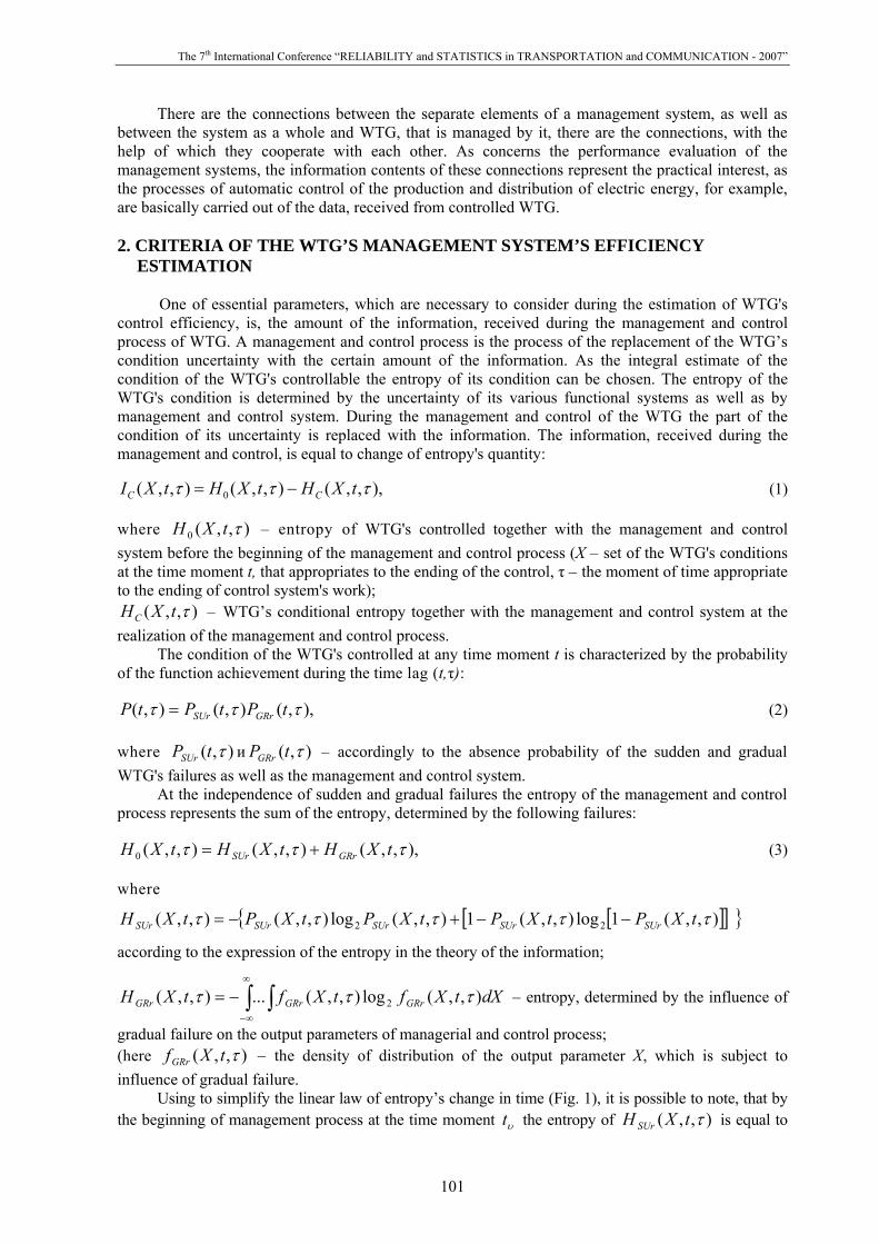
The 7th International Conference “RELIABILITY and STATISTICS in TRANSPORTATION and COMMUNICATION - 2007”
101
There are the connections between the separate elements of a management system, as well as between the system as a whole and WTG, that is managed by it, there are the connections, with the help of which they cooperate with each other. As concerns the performance evaluation of the management systems, the information contents of these connections represent the practical interest, as the processes of automatic control of the production and distribution of electric energy, for example, are basically carried out of the data, received from controlled WTG.
2. CRITERIA OF THE WTG’S MANAGEMENT SYSTEM’S EFFICIENCY
ESTIMATION
One of essential parameters, which are necessary to consider during the estimation of WTG's control efficiency, is, the amount of the information, received during the management and control process of WTG. A management and control process is the process of the replacement of the WTG’s condition uncertainty with the certain amount of the information. As the integral estimate of the condition of the WTG's controllable the entropy of its condition can be chosen. The entropy of the WTG's condition is determined by the uncertainty of its various functional systems as well as by management and control system. During the management and control of the WTG the part of the condition of its uncertainty is replaced with the information. The information, received during the management and control, is equal to change of entropy's quantity:
),,,(),,(),,( 0 τττ tXHtXHtXI CC −= (1)
where ),,(0 τtXH – entropy of WTG's controlled together with the management and control system before the beginning of the management and control process (X – set of the WTG's conditions at the time moment t, that appropriates to the ending of the control, τ – the moment of time appropriate to the ending of control system's work);
),,( τtXHC – WTG’s conditional entropy together with the management and control system at the realization of the management and control process.
The condition of the WTG's controlled at any time moment t is characterized by the probability of the function achievement during the time lag (t,τ):
),,(),(),( τττ tPtPtP GRrSUr= (2)
where ),( τtPSUr и ),( τtPGRr – accordingly to the absence probability of the sudden and gradual WTG's failures as well as the management and control system.
At the independence of sudden and gradual failures the entropy of the management and control process represents the sum of the entropy, determined by the following failures:
),,,(),,(),,(0 τττ tXHtXHtXH GRrSUr += (3)
where
{ [ ][ ] }),,(1log),,(1),,(log),,(),,( 22 τττττ tXPtXPtXPtXPtXH SUrSUrSUrSUrSUr −−+−=
according to the expression of the entropy in the theory of the information;
dXtXftXftXH GRrGRrGRr ),,(log),,(...),,( 2 τττ ∫ ∫∞
∞−
−= – entropy, determined by the influence of
gradual failure on the output parameters of managerial and control process; (here ),,( τtXfGRr – the density of distribution of the output parameter X, which is subject to influence of gradual failure.
Using to simplify the linear law of entropy’s change in time (Fig. 1), it is possible to note, that by the beginning of management process at the time moment υt the entropy of ),,( τtXH SUr is equal to

Session 2. Statistical Methods and Their Applications
102
the some value of ),,( τυtXH SUr , but the entropy: ),,(),,(),,( 00 τττ υtXHtXHtXH SUrGRr −= . During the time in the absence thereof management and control the uncertainty of the WTG’s as well as management and control system’s condition are continuously growing, and as the result the entropy too.
Figure 1. Change of the WTG’s entropy ignoring and considering the management and control process
The management and control process, carried out in the time range ),( ccc TT τ+ , reduces the uncertainty of the managed WTG. The control can be carried out continuously or, as it is shown on Fig. 1, discretely with the frequency cT/1 , which is chosen from the condition of the adequacy of time to reduce the uncertainty up to the given level. The optimum level of the managed WTG’s uncertainty is chosen according to the condition of the adjusted probability of WTG’s function achievement assurance:
{
[ ] [ ] },),,(1log),,(1
),,(log),,(),,(
2
2
WacacWacac
WacacWacacopt
tXPtXP
TXPtXPtXH
ττ
τττ
−−+
+−= (4)
where ),,( WacactXP τ – is the probability of WTG’s as well as management and control system’s
function achievement in the time range ),( Wacact τ , which beginning is the time moment of the
control ending act (the end of the control), and the end – the time moment of the management cycle ending during the work of WTG Wacτ (the end of a WTG’s management cycle). Time of monitoring
procedure cτ should be shown to a minimum, to get as possible more reliable information per time unit. At the same time this minimum should not exceed allowable time of WTG’s putting out of operation, as it results the unnecessary complication of the management and control system.
The real devices of monitoring systems, as well as real algorithms of the control, have some loss of the information during the control process. The total losses of the information are connected with two kinds of mistakes of the monitoring system during its work. The first ones are the undetectable failures, and the second – the so-called fictitious failures.
By the meaning of the undetectable failures are mentioned such failures, that are not found out during the control owing to the final accuracy of the algorithm as well as management and control system.
By the meaning of the fictitious failures there are mentioned actually absent failures, which are falsely found out during the control as the result of insufficient accuracy of the algorithm and checked devices.
During the management and control of the WTG the set of parameters т is exposed to measurement. The probability of existence at least one undetectable failure in a series of the т parameters measurement can be determined according the formula:
H(X,t,τ)
H0
HGRr
Hopt
HSU
t0 1Tc Tc + τc 2Tc 3Tc topt
t

The 7th International Conference “RELIABILITY and STATISTICS in TRANSPORTATION and COMMUNICATION - 2007”
103
[ ].),(11),(1
∏=
−−=m
iundiund tPtP ττ (5)
At equal probabilities of the undetectable failures the formula (5) will become as follows:
[ ] .),(11),( mundiund tPtP ττ −−= (6)
The probability of existence at least one false failure in a series of the т parameters
measurement can be determined according the formula:
[ ].),(11),(1
∏=
−−=m
ifaifa tPtP ττ (7)
At equal probabilities of the false failures the formula (7) will become as follows:
[ ] .),(11),( mfaifa tPtP ττ −−= (8)
The probabilities ),( τtPundi and ),( τtPfai are determined, depending on the distribution laws of
the controllable parameters and errors of the WTG’s devices. Thus according to the normal distribution laws the expression of the probability density of the controllable parameters and errors of the monitoring system’s devices look like
;2
)(exp2
1),,( 2
2
⎥⎦
⎤⎢⎣
⎡ −−=
XXC
XxtXfσπσ
τ (9)
2exp
21),,( 2
2
⎥⎦
⎤⎢⎣
⎡−=
ZZEr
ZtXfσπσ
τ . (10)
According to the expressions (9) and (10) the probabilities ),( τtPundi and ),( τtPfai can be
determined by the formulas
;2
)(exp2222
1
2)(exp
22221),(
2
2
2
2
dxXxxaxb
dxXxxaxbtP
Xb ZZ
X
a
ZXXundi
⎥⎦
⎤⎢⎣
⎡ −−×
⎥⎥⎦
⎤
⎢⎢⎣
⎡⎟⎟⎠
⎞⎜⎜⎝
⎛ −Φ−⎟⎟
⎠
⎞⎜⎜⎝
⎛ −Φ+
+⎥⎦
⎤⎢⎣
⎡ −×
⎥⎥⎦
⎤
⎢⎢⎣
⎡⎟⎟⎠
⎞⎜⎜⎝
⎛ −Φ−⎟⎟
⎠
⎞⎜⎜⎝
⎛ −Φ=
∫
∫∞
∞−
σσσπσ
σσσπστ
(11)
,22
22
)(exp22
1),( 2
2
dxxbxaXxtPZZ
b
a XXfai
⎥⎥⎦
⎤
⎢⎢⎣
⎡⎟⎟⎠
⎞⎜⎜⎝
⎛ −Φ−⎟⎟
⎠
⎞⎜⎜⎝
⎛ −Φ+×⎥
⎦
⎤⎢⎣
⎡ −−= ∫ σσσπσ
τ (12)
where x and X – a controlled variable and its average value accordingly;
Z – a mistake of the monitoring system device; Xσ and Zσ – the roof-mean-square deviations of the X parameter and Z mistake;
а, b – previously legitimate values of the X parameter; Ф(а, b, х, Zσ ) – La Plasa function.

Session 2. Statistical Methods and Their Applications
104
Knowing the ),( τtPundi and ),( τtPfai probabilities, according to the absolute probability theorem it is possible to determine the probability of WTG’s function achievement considering the errors of the monitoring system’s work:
[ ]
[ ] [ ]),(1),(),(1),(),(1),(
),(00
0
ττττττ
τtPtPtPtP
tPtPtP
undfa
fa
−+−−
= , (13)
where Р0(t,τ) – a probability of the WTG’s up state. Knowing the probability of achievement of functions by WTG’s, considering the work of
monitoring system, it is possible to estimate its remaining entropy after the т parameter’s control:
∑=
=m
ii tHtH
100 ),,(),( ττ
where [ ] [ ]{ }),(1log),(1),(log),(),( 220 τττττ tPtPttPtH iiii −×−+−= – the entropy, which remains after the control of one (i-th) parameter.
The other parameters, which is also necessary to be considered during the estimation of WTG’s control process efficiency, are the realization costs of the control. For all that, the average cost of monitoring system operation will be determined according to the formula:
[ ] ,),(1),(),( 0
COpertPtCbtC OperOperOperατττ −= (14)
where Operb – the factor, determined during the operation (0≤ Operb ≤1) ;
),(0 τtC Oper – the cost of the elementary monitoring system’s operation, which probability of
non-failure operation is lower, than the required quantity is ),( τtP ;
COperα – the constant parameter, determined during the operation of the monitoring system. Further for the equal estimation of the various WTG’s management and control systems the
special generalized functional-statistical criterion of the process and management system’s efficiency estimation is offered to be developed. For all that the generalized criterion of the efficiency evaluation has to characterize the information ability of the process as well as the management and control system.
The information quantity, that is got by the monitoring system during the WTG’s control and management for the time lag ( t , τ ) , is determined according to the following dependence:
),(),(),( 0 τττ tHtHtI −= , (15)
where ),(0 τtH – entropy, which characterizes the uncertainty of the monitoring system, that
controls the WTG before the beginning of the management and control process, is determined according to the formula (3);
),( τtH – remaining entropy of the controlled WTG and monitoring system after realization of the WTG’s management and control is determined by the formula (4).
The equality (15) characterizes the real information opportunity of the control system. The potential opportunity of a control and management system makes the value
),(),( 0 ττ tHtIP = . (16)
The control system effectiveness like information can be estimated by the criterion:

The 7th International Conference “RELIABILITY and STATISTICS in TRANSPORTATION and COMMUNICATION - 2007”
105
,),(),(),(
ττ
τtItItE
P
RI = (17)
where ),(),( ττ tItI R = – the real quantity of information, determined in (15). Considering (15) and (16) to estimate the control system effectiveness, we will get the expression:
.),(
),(),(),(
0
0
τττ
τtH
tHtHtE
−= (18)
By the expression (18) it is easy to notice, that the ideal monitoring system will have the
efficiency value 1),( =τtEI , but the real one – the value of 1),( <τtEI . However, the criterion (18) does not consider the dynamics of the management and control process, as well as the, complexity and the cost of the monitoring system. The failings, which are marked in criterion (18), can be removed by the entering another ratio for the control system effectiveness:
,),(),(),(
0 ττ
τtktktE
I
I= (19)
where ),(),(),( max
τττ
tCtItkI
Σ
= – maximum information, received by the monitoring system, per unit of
its total cost. Here:
∑=
=m
ii tItI
1maxmax ),(),( ττ – maximum information, received during the control process of the т
parameters;
),(),(
),(min
maxmax0 τ
ττ
tCtI
tkI = – the maximal average quantity of the information, received by the
monitoring system during the control or the process according т parameters per unit of the minimal total cost of the idealized monitoring system. Here:
∑=
=m
ii tItI
1maxmaxmaxmax ),(),( ττ – maximal average amount of the information received at the
WTG’s control according to the т parameters.
Taking into account the ratios (15), (16), (19), considered above, and the equality mtI =),(maxmax τ , we receive the final formula for the estimation of the control system
effectiveness:
[ ]
∑
∑
=
=
⋅−= m
ii
m
iioi
tCm
tCtHtHtE
1
1min
),(
),(),(),(),(
τ
ττττ . (20)
Thus, for the estimation of the management and control process efficiency, which is carried out
by the monitoring system, it is necessary: - to determine each WTG’s subsystem entropy, as well as the monitoring system before the
realization of control process; - to determine the entropy of the controlled WTG considering the entropy of the control system,,
which is determined by the mistakes, during the management and control process of each WTG’s subsystem realization;

Session 2. Statistical Methods and Their Applications
106
- to count up the initial cost minC and the final cost C of the monitoring system; - to clear using the formula (20).
Let's notice, that the range of the generalized statistical criterion change corresponds to the condition
.1),(0 ≤≤ τtE
Therefore, the more perfectly and highly effectively is the monitoring system, the more generalized parameter of efficiency will aspire to the unit.
3. PRACTICAL EXAMPLE
Further with the purpose of the illustration of the offered technique we will estimate the management and control system effectiveness, which is executed on the basis of MITA WindPower Management System (WPMS) controller [2], with the use of the offered criterion for concrete WTG such as NORDEX N54.
We will determine the initial data, which are necessary for the estimation of the control process, from the operational documentation of the WTG N54 [3,4]. As an example we will assume, that during the control the estimation will be done at the uniformly precise control of five WTG’s parameters, which have the identical roof-mean-square deviations 1,0=iσ and identical tolerance
25,0=Δ i at the identical reliability of the controllable elements 9,00 =iP . It is known, that the controller’s roof-mean-square deviations of the control of each parameter is 025,0=icsσ . The
economic parameters of the controller (the cost and the factor, considering the cost of service per control’s time unit, are determined during the operational process [5]) make the values 1000=csC € and 10=Operα €/minutes accordingly. The time of the total control of the WTG’s chosen parameters
is 2,0=cT minutes. Further, using the received data, according to the technique, offered above, the following
operations will be done: 1. We find the value of the WTG’s as well as controller’s entropy according to the control of
one parameter, using the set point iP0 and Table 1. We have 4691,00 =iH .
Table 1. The values of the probabilities of the given function activities by the controlled WTG at the i-th parameter and the values of entropy appropriate to them
Pi Hi Pi Hi 0,01 0,0808 0,55 0,9927 0,02 0,1415 0,60 0,9709 0,03 0,1949 0,65 0,9341 0,04 0,2422 0,70 0,8814 0,05 0,2864 0,75 0,8113 0,06 0,3274 0,80 0,7219 0,07 0,3659 0,85 0,6099 0,08 0,4021 0,90 0,4691 0,09 0,4366 0,91 0,4366 0,10 0,4691 0,92 0,4021 0,15 0,6099 0,93 0,3659 0,20 0,7219 0,94 0,3274 0,25 0,8113 0,95 0,2864 0,30 0,8814 0,96 0,2422 0,35 0,9341 0,97 0,1949 0,40 0,9709 0,98 0,1415 0,45 0,9927 0,99 0,0808 0,50 1,0000 1,00 0,0000

The 7th International Conference “RELIABILITY and STATISTICS in TRANSPORTATION and COMMUNICATION - 2007”
107
2. We determine the value of the WTG‘s entropy and controller according to the control of five parameters:
∑=
=⋅==5
100 .3455,24691,05
iiHH
3. We determine the following:
- a limiting error of the controller at the control of the i-th parameter: ;075,0025,033 =⋅== icsi σδ
- a relative value of a limiting error:
;3,025,0
075,0==
Δ=
i
iiz
δ
- a relative value of the tolerance to the i-th parameter:
;5,21,025,0
==Δ
=i
iir σ
the relation of a limiting error of the controller at the control i-th parameter to a root-mean-square deviation i-th parameter:
.75,01,0
075,0==
i
i
σδ
4. We determine the probabilities of undetectable and fictitious failures, using the nomograms
(Fig. 2, 3). We have 006,02 == undiundi fP and .003,02 == faifai fP
Figure 2. The nomogram of the dependence ⎟⎟
⎠
⎞⎜⎜⎝
⎛zrf
Xfa ,
σδ
5. We determine a posteriori probability of the WTG’s functions performance according to the i-th parameter, using faiundi PP , values and the following formula:
)1()1()1(
00
0
iundifaii
faiii PPPP
PPP
−+−−
= .
We receive Рi = 0,9993.
Xσδ
⎟⎟⎠
⎞⎜⎜⎝
⎛zrf
Xfa ,
σδ
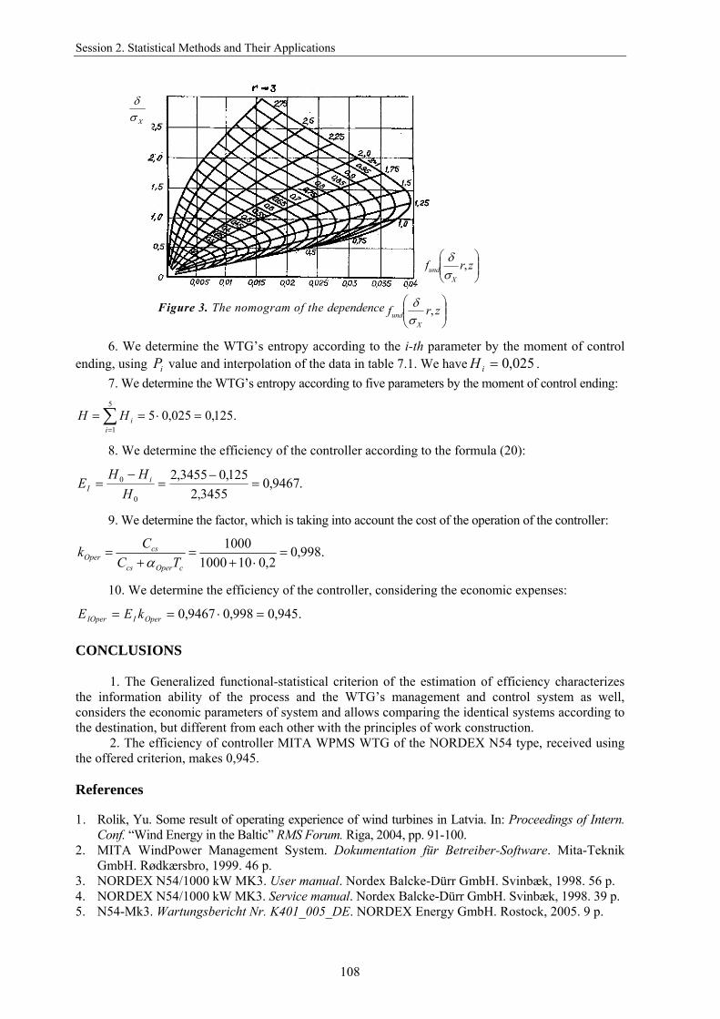
Session 2. Statistical Methods and Their Applications
108
Figure 3. The nomogram of the dependence
⎟⎟⎠
⎞⎜⎜⎝
⎛zrf
Xund ,
σδ
6. We determine the WTG’s entropy according to the i-th parameter by the moment of control ending, using iP value and interpolation of the data in table 7.1. We have 025,0=iH .
7. We determine the WTG’s entropy according to five parameters by the moment of control ending:
∑=
=⋅==5
1.125,0025,05
iiHH
8. We determine the efficiency of the controller according to the formula (20):
.9467,03455,2
125,03455,2
0
0 =−
=−
=H
HHE i
I
9. We determine the factor, which is taking into account the cost of the operation of the controller:
.998,02,0101000
1000=
⋅+=
+=
cOpercs
csOper TC
Ckα
10. We determine the efficiency of the controller, considering the economic expenses:
.945,0998,09467,0 =⋅== OperIIOper kEE
CONCLUSIONS
1. The Generalized functional-statistical criterion of the estimation of efficiency characterizes the information ability of the process and the WTG’s management and control system as well, considers the economic parameters of system and allows comparing the identical systems according to the destination, but different from each other with the principles of work construction.
2. The efficiency of controller MITA WPMS WTG of the NORDEX N54 type, received using the offered criterion, makes 0,945.
References
1. Rolik, Yu. Some result of operating experience of wind turbines in Latvia. In: Proceedings of Intern.
Conf. “Wind Energy in the Baltic” RMS Forum. Riga, 2004, pp. 91-100. 2. MITA WindPower Management System. Dokumentation für Betreiber-Software. Mita-Teknik
GmbH. Rødkærsbro, 1999. 46 p. 3. NORDEX N54/1000 kW MK3. User manual. Nordex Balcke-Dürr GmbH. Svinbæk, 1998. 56 p. 4. NORDEX N54/1000 kW MK3. Service manual. Nordex Balcke-Dürr GmbH. Svinbæk, 1998. 39 p. 5. N54-Mk3. Wartungsbericht Nr. K401_005_DE. NORDEX Energy GmbH. Rostock, 2005. 9 p.
Xσδ
⎟⎟⎠
⎞⎜⎜⎝
⎛zrf
Xund ,
σδ

The 7th International Conference “RELIABILITY and STATISTICS in TRANSPORTATION and COMMUNICATION - 2007”
109
FINDING SAMPLING DISTRIBUTIONS AND RELIABILITY ESTIMATORS FOR TRUNCATED LAWS
VIA UNBIASEDNESS EQUIVALENCE PRINCIPLE
Nicholas A. Nechval1, Konstantin N. Nechval2, Gundars Berzins1, Maris Purgailis1, Juris Krasts1, Uldis Rozevskis1, Kristine Rozite1, Vladimir Strelchonok3, Natalie Zolova1
1Mathematical Statistics Department, University of Latvia
Raina Blvd 19, Riga, LV-1050, Latvia E-mail: [email protected]
2Mathematical Methods and Modelling Department, Transport and Telecommunication Institute
Lomonosova 1, Riga, LV-1019, Latvia E-mail: [email protected]
3Informatics Department, Baltic International Academy
Lomonosova 1, Riga, LV-1019, Latvia E-mail: [email protected]
In this paper, the problem of finding sampling distributions for truncated laws is considered. This problem concerns the very important area of information processing in Industrial Engineering. It remains today perhaps the most difficult and important of all the problems of mathematical statistics that require considerable efforts and great skill for investigation. The technique discussed here is based on use of the unbiasedness equivalence principle, the idea of which belongs to the authors, and often provides a neat method for finding sampling distributions. It avoids explicit integration over the sample space and the attendant Jacobian but at the expense of verifying completeness of the recognized family of densities. Fortunately, general results on completeness obviate the need for this verification in many problems involving exponential families. The proposed technique allows one to obtain results for truncated laws via the results obtained for non-truncated laws. It is much simpler than the known techniques. The examples are given to illustrate that in many situations this technique allows one to find the results for truncated laws and to estimate system reliability in a simple way.
Keywords: truncated law, sampling distribution, unbiasedness equivalence principle, reliability estimation 1. INTRODUCTION
The truncated distributions have found many applications. Several examples have been given employing the truncated distributions in fitting rainfall data and animal population studies where observations usually begin after migration has commenced or concluded before it has stopped [1-2]. Similar situations arise with regard to aiming errors (range, deflection, etc.) in gunnery and other bombing accuracy studies. For example, in gun camera missions, the view angle of the camera defines a known truncation point for an exponentially distributed random variable, observable as some function of the radial error or the distance from the aiming point to the point of impact [3]. A situation for the truncated Poisson distribution would occur when one wishes to fit a distribution to Poisson-like data consisting of numbers of individuals in certain groups which posses a given attribute, but in which a group cannot be sampled unless at least a specified number of its members have the attribute. For example, the group may be a household of people, and the attribute measles; the specified number would then be one. Other examples arise in life testing and reliability problems, where if failure is caused by a wear-out mechanism or is a consequence of accumulated wear, then the length-of-life of a system can be expected to be of finite dimension. The object of the present paper is to obtain a sampling distribution for truncated law with a known truncation point and a minimum variance unbiased estimator of the reliability function for this model using the results obtained for non-truncated law. It is known that a sampling distribution for truncated law may be derived using, namely, the method based on characteristic functions [4], the method based on generating functions

Session 2. Statistical Methods and Their Applications
110
[5], or the combinatorial method [6]. In this paper, a much simpler technique than the above-mentioned is proposed. It allows one to obtain the results for truncated laws more easily. 2. UNBIASEDNESS EQUIVALENCE PRINCIPLE
Suppose an experiment yields data sample Xn = (X1, … , Xn) relevant to the value of a parameter θ (in general, vector). Let LX(xn;θ) denote the probability or probability density of Xn when the parameter assumes the value θ. Considered as a function of θ for given Xn=xn, LX(xn;θ) is the likelihood function. If the data sample Xn can be summarized by a sufficient statistic S, one can write LS(s;θ) ∝ LX(xn;θ). Further, for any non-negative function ω (s), ω (s)LS(s;θ) is also a likelihood function equivalent to LX(xn;θ). Suppose we recognize a function ω (s) such that ω (s)LS(s;θ), regarded as a function of s for a given θ, is a density function. It can be shown that this is the sampling density of S if the family of recognized densities is complete.
The unbiasedness equivalence principle consists in the following. If LX(xn;θ,ϑ)=[w(θ,ϑ,)]nLX(xn;θ), (1) represents the likelihood function for the truncated law, where w(θ,ϑ) is some function of a parameter (θ,ϑ) associated with truncation, ϑ is a known truncation point (in general, vector), then a sampling density for the truncated law is determined by
[ ] , ),;()()();( ϑϑ ϑ S∈= ssss θθ,θ gwwg n (2)
where
[ ] );()()( θθ ss gww nϑ, = ϕ(s)LS(s;θ,ϑ) ∝ LX(xn;θ,ϑ), (3) g(s;θ) is a sampling density of a sufficient statistic s(Xn) (for a family of densities {f(x;θ)}) determined on the basis of LX(Xn;θ), )(Sw is an unbiased estimator of 1/[w(θ,ϑ)]n with respect to g(s;θ), s∈S (a sample space of a non-truncated sufficient statistic S), ϕ(S) is a function of S for a given θ, which is equivalent to unbiased estimator )(Sw of 1/[w(θ,ϑ)]n, i.e., ϕ(S) ∝ )(Sw (4) or ϕ(S) = [ ] ),;(/);(),()( ϑϑ θθθ SSS SLgww n , (5) g(s;θ,ϑ) is the sampling density of a sufficient statistic S (for a family of densities {fϑ (x;θ)}) when the truncation parameter ϑ is known, Sϑ is a sample space of a truncated sufficient statistic S. 3. ILLUSTRATIONS OF THE UNBIASEDNESS EQUIVALENCE PRINCIPLE
Example 3.1 (Sampling distribution for the left-truncated Poisson law). Let the Poisson probability function be denoted by
. ... 2, 1, 0, ,!
);( == − xex
xfx
θθθ (6)
The probability function of the restricted random variable, which is truncated away from some ϑ≥0, is then
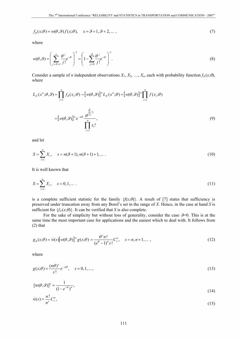
The 7th International Conference “RELIABILITY and STATISTICS in TRANSPORTATION and COMMUNICATION - 2007”
111
, ... 2, 1, ),;(),();( ++== ϑϑθϑθθϑ xxfwxf (7) where
.!
1!
),(1
0
1
1
−
−
=
−
−∞
+=⎟⎟⎠
⎞⎜⎜⎝
⎛−=
⎟⎟⎠
⎞⎜⎜⎝
⎛= ∑∑ θ
ϑθ
ϑ
θθϑθ ej
ej
wj
j
j
j
(8)
Consider a sample of n independent observations X1, X2, …, Xn, each with probability function fϑ (x;θ), where
∏=
=n
ii
nX xfxL
1
);(),;( θϑθ ϑ [ ] [ ] ∏=
==n
ii
nnX
n xfwxLw1
);(),();(),( θϑθθϑθ
[ ] ,!
),(
1
1
∏=
−
∑=
= n
ii
x
nn
xew
n
ii
θϑθ θ (9)
and let
. ... ,1)1( ),1( ,1
∑=
+++==n
ii nnsXS ϑϑ (10)
It is well known that
... 1, 0, ,1
== ∑=
sXSn
ii . (11)
is a complete sufficient statistic for the family {f(x;θ)}. A result of [7] states that sufficiency is preserved under truncation away from any Borel’s set in the range of X. Hence, in the case at hand S is sufficient for {fϑ (x;θ)}. It can be verified that S is also complete.
For the sake of simplicity but without loss of generality, consider the case ϑ=0. This is at the same time the most important case for applications and the easiest which to deal with. It follows from (2) that
[ ] );(),()();( θϑθθϑ sgwswsg n= , ... 1, , ,! )1(
! +=
−= nnsC
sen n
sn
s
θθ (12)
where
, ... 1, 0, ,! )();( == − se
snsg n
sθθθ (13)
,)1(
1)],[w( nn
e θϑθ −−=
(14)
,! )( nss C
nnsw =
(15)
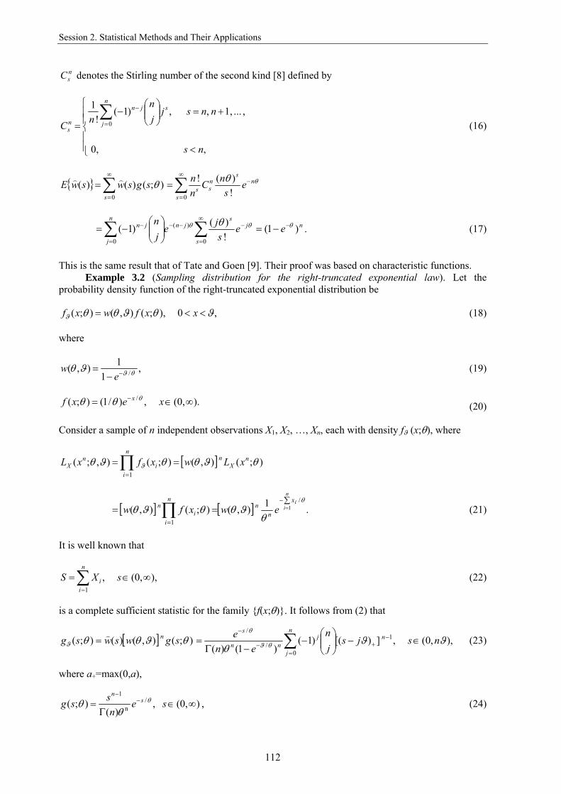
Session 2. Statistical Methods and Their Applications
112
nsC denotes the Stirling number of the second kind [8] defined by
⎪⎪⎩
⎪⎪⎨
⎧
<
+=⎟⎟⎠
⎞⎜⎜⎝
⎛−
=∑
=
−
, 0,
, ... 1, , ,)1(!
1
0
ns
nnsjjn
nC
n
j
sjn
ns (16)
{ } ∑∞
=
=0
);()()(s
sgswswE θ θθ ns
s
nss e
snC
nn −
∞
=∑=
! )(!
0
∑ ∑=
−∞
=
−−−− −=⎟⎟⎠
⎞⎜⎜⎝
⎛−=
n
j
n
s
js
jnjn eesje
jn
0 0
)( )1(! )()1( θθθ θ . (17)
This is the same result that of Tate and Goen [9]. Their proof was based on characteristic functions.
Example 3.2 (Sampling distribution for the right-truncated exponential law). Let the probability density function of the right-truncated exponential distribution be
,0 ),;(),();( ϑθϑθθϑ <<= xxfwxf (18) where
,1
1),( /θϑϑθ −−=
ew (19)
).(0, ,)/1();( / ∞∈= − xexf x θθθ (20)
Consider a sample of n independent observations X1, X2, …, Xn, each with density fϑ (x;θ), where
[ ] );(),();(),;(
1
θϑθθϑθ ϑn
Xn
n
ii
nX xLwxfxL == ∏
=
[ ] [ ] .1),();(),(/
1
1θ
θϑθθϑθ
∑=
−
=∏ ==
n
iix
nn
n
ii
n ewxfw (21)
It is well known that
),(0, ,1
∞∈= ∑=
sXSn
ii (22)
is a complete sufficient statistic for the family {f(x;θ)}. It follows from (2) that
[ ] );(),()();( θϑθθϑ sgwswsg n= ,),0( ,])[()1()1()( 0
1 /
/
ϑϑθ θϑ
θ
nsjsjn
ene n
j
njnn
s
∈−⎟⎟⎠
⎞⎜⎜⎝
⎛−
−Γ= ∑
=
−+−
−
(23)
where a+=max(0,a),
, )(0, ,)(
);( /n
1
∞∈Γ
= −−
sen
ssg sn
θ
θθ (24)

The 7th International Conference “RELIABILITY and STATISTICS in TRANSPORTATION and COMMUNICATION - 2007”
113
,)1(
1)],([ /
nn
ew θϑϑθ −−
= (25)
,])[()1(1(s)0
1 1 ∑
=
−+− −⎟⎟
⎠
⎞⎜⎜⎝
⎛−=
n
j
njn js
jn
sw ϑ (26)
{ } dssgswswE );()()(0
θ∫∞
= ∫∑∞
+−−
−+−
=
−Γ−
⎟⎟⎠
⎞⎜⎜⎝
⎛−=
0
/)(1
/
0
)()(
])[()1( ϑθ
ϑ θϑθϑ jsdenjse
jn js
n
nj
n
j
j .)1( / ne θϑ−−= (27)
4. VALIDITY OF THE UNBIASEDNESS EQUIVALENCE PRINCIPLE
The theoretical results of this investigation into the validity of the proposed unbiasedness equivalence principle (UEP) for finding sampling distributions for truncated laws are largely contained in the theorem given below. We introduce the following notation and assumptions. Let Xn be a random variable taking on values xn in a space Xϑ, let A be a σ −field of subsets of Xϑ, and let (θ,ϑ) be a parameter associated with truncation, where ϑ is a known truncation point. For all values of the parameter θ in some parameter space Θ, let Pϑ be a probability measure on A; i.e., for any set A in A, Pϑ (A;θ) is the probability that Xn will belong to A when the parameter has the value θ. Let S=s(Xn) be a statistic on the measurable space (Xϑ,A ) taking on values in a measurable space (Sϑ, B). For each θ∈Θ, let Gϑ be the probability distribution of S when Xn has the distribution Pϑ; i.e., for any B∈B, Gϑ(B;θ) = Pϑ( ),);(1 θB−s where s-1(B) is the set of points xn in Xϑ for which s(xn)∈B.
(i) Assume the family P = {Pϑ: θ∈Θ} of probability distributions of Xn is dominated by a totally σ −finite measure μ over (Xϑ,A), i.e., there exists, for all θ∈Θ, a non-negative A – measurable function pϑ (xn;θ) such that
∫A
nn xdxpAP )();(= );( μϑϑ θθ (28)
for all A∈A. (The integrand pϑ(xn;θ) is called the density of Pϑ w.r.t. (with respect to) μ).
(ii) Assume that s(Xn) is sufficient for P. From the Halmos-Savage’s factorisation theorem [10], s(Xn) is sufficient if and only if for each θ∈Θ there exists a non-negative B-measurable function LS(s(xn);θ,ϑ) on Sϑ and a non-negative A – measurable function v on Xϑ such that
).( )(),);(( = );( μϑϑnnn xvxLxp θθ sS (29)
(The symbol (μ) following a statement means that the statement holds except on a set of μ-measure zero). In (28), we will assume that LS and v are finite (μ).
(iii) Assume we recognize some likelihood function LS(s;θ,ϑ) equivalent to likelihood function LX(xn;θ,ϑ). Define a σ −finite measure ρ over (Xϑ,A) by
∫ ∈A
nn AxdxvA A. all ,)()( = )( μρ (30)
Then, from (28), (29), and (30),
∫ ∈A
nn AxdxLAP A. all ,)(),);(( = );( ρϑϑ θθ sS (31)
Session 2. Statistical Methods and Their Applications
114
(iv) Assume we recognize a totally σ −finite measure η over (Sϑ, B) such that the measure ρ s-1 over (Sϑ, B) is absolutely continuous w.r.t. η; i.e., η(B)=0 implies that ρ s-1(B)=0, where ρ s-1(B) denotes the ρ − measure of the inverse image of B.
(v) Assume we recognize a positive B-measurable function ϕ on Sϑ such that
∫ ≡ϑ
ηϕϑS
1)()(),;( sssS dL θ (32)
for all θ∈Θ. Assume further that for any measurable set B of positive η − measure, there exists a θ∈Θ and a measurable subset B1 of B of positive η − measure over which LS(s;θ,ϑ)ϕ(s) is positive.
From (32), {LS(s;θ,ϑ)ϕ(s):θ∈Θ} is a family of densities w.r.t. η. For B∈B, let
∫=B
dLBG ).()(),;();( sssS ηϕϑθϑ θ (33)
Thus, (v) provides us with a family of densities, but at this stage we do not know if this recognized family is the family of sampling densities of S.
(vi) Assume we recognize that the family {LS(s;θ,ϑ)ϕ(s):θ∈Θ} is complete, i.e.,
∫ ∈≡ϑ
ηϕϑφS
Θθθ allfor 0)()(),;()( ssss S dL (34)
implies
0 )( ≡sφ (35) except on a set D with 0);( =θDGϑ for all θ∈Θ.
Theorem 1 (Sampling distribution for truncated law). Under assumptions (i) through (vi), Gϑ has a density with respect to η and LS(s;θ,ϑ)ϕ(s) is a version of it, i.e., LS(s;θ,ϑ)ϕ (s) = [ ] );(),()( θθ ss gww nϑ (36) is the sampling density, gϑ (s;θ) of the sufficient statistic s(Xn).
Proof. We show first that (35) and the second part of (v) imply that φ (s)≡0 (η). For suppose there exists a measurable В with η(B)>0 and φ(s)≠0 over B. Then B⊂D, so Gϑ(B;θ)=0 for all θ∈Θ. But, from (v), there exists a B1⊂B for which Gϑ (B1;θ)>0 for some θ, contradicting Gϑ (B;θ)=0 for all θ∈Θ. Now, by a theorem in [10], there exists a non-negative measurable function ψ on Sϑ such that
∫∫ = )()();()());(( ssss ηψρ ϑϑ dQxdxQ nn θθ (37)
for every measurable function Qϑ, in the sense that if either integral exists, then so does the other and the two are equal. In (37), let Qϑ (s,θ) =χBLS(s;θ,ϑ), where χB is the characteristic function of B (B∈B). Then there exists a ψ (s) such that
∫∫ =− BB
nn dLxdxL )()(),;()(),);(()(1
ssss S
s
S ηψϑρϑ θθ (38)
for all B∈B. Note that the left side of (37) is Gϑ(B;θ).
In (34), let φ (s) = 1−[ψ(s)/ϕ (s)]. From (32) and (38),
The 7th International Conference “RELIABILITY and STATISTICS in TRANSPORTATION and COMMUNICATION - 2007”
115
∫ =⎥⎦
⎤⎢⎣
⎡−
ϑ
ηϕϑϕψ
S
0)()(),;()()(1 sss
ss
S dL θ (39)
for all θ∈Θ. Thus, from (35), ψ(s)=ϕ(s) almost everywhere (η), and, from (37), LS(s;θ,ϑ)ϕ(s) = [ ] );(),()( θθ ss gww nϑ (40) is a version of the density of Gϑ with respect to η. ˛
Theorem 2 (Continuous multidimensional case). Let X be a multidimensional random variable with density function fϑ(x;θ), where θ is a parameter vector which ranges over a parameter space Θ, ϑ is a known truncation point vector. Let Xn=(X1, …, Xn) be a random sample and S=S(Xn) be a statistic sufficient for θ. Assume we have found L(s;θ,ϑ), the likelihood function, in terms of the sufficient statistic S that has a sampling density g(s;θ). Suppose we recognize a positive function ϕ (s) such that L(s;θ,ϑ)ϕ (s) = [ ] );(),()( θϑθ ss gww n (41) (where w(θ,ϑ) is some function of a parameter (θ,ϑ) associated with truncation, )(Sw is an unbiased estimator of 1/[w(θ,ϑ)]n with respect to g(s;θ), s∈S (a sample space of a non-truncated sufficient statistic S)), is interpretable as a density function, gϑ (s;θ), of S, i.e., if
1)(),;( =∫ sss dL ϕϑθ for all θ∈Θ, (42)
where the integration is over the truncated space of S. Then (40) is the sampling density of S, if the family of densities {L(s;θ,ϑ)ϕ (s): θ∈Θ} is complete, i.e.,
1)(),;()( =∫ ssss dL ϕφ ϑθ for all θ∈Θ (43)
implies that φ(s) must be zero with probability one.
Proof. Let gϑ (s;θ) denote the sampling density of S. Then gϑ (s;θ) ∝ L(s;θ,ϑ) ∝ L(s;θ,ϑ)ϕ (s). (44) Suppose that ψ(s) is any non-negative function such that
1)(),;( =∫ sss dL ψϑθ for all θ∈Θ. (45)
Then
∫ =⎥⎦
⎤⎢⎣
⎡− 0),;()(
)()(1 sss
ss dL ϑθϕ
ϕψ for all θ∈Θ, (46)
and it follows from the assumed completeness that ψ(s)=ϕ(s) with probability one. Hence, gϑ (s;θ)= ϕ (s)L(s;θ,ϑ) = [ ] );(),()( θϑθ ss gww n , (47) which completes the proof. ˛

Session 2. Statistical Methods and Their Applications
116
5. FINDING RELIABILITY ESTIMATORS FOR TRUNCATED LAWS VIA THE UNBIASEDNESS EQUIVALENCE PRINCIPLE
Consider a system that is required to operate for a given ‘mission time’, t. The reliability of this system for the right-truncated distribution of time-to-failure with the probability density function fϑ
(x;θ) may be defined as
∫=≥=ϑ
ϑt
dxxftxtR .);()Pr()( θ (48)
Due to the Rao-Blackwell’s and Lehmann-Scheffé’s theorem [11] a minimum variance unbiased (MVU) estimator for R may be obtained as
∫=ϑ
ϑt
dxxftR ,);()( s (49)
where X may be any one of the observations (X1, …, Xn) from fϑ (x;θ), S is a complete sufficient statistic for {fϑ (x;θ)}, and fϑ (x;s) is the conditional distribution of X given S=s; fϑ (x;s) is obtained as
,)(
),,();();,();(
ssss
wxw
gxfxf f ϑ
ϑ
ϑϑ
θθθ
== (50)
where
);()],()[,,();,( θθθθ ss gwxwxf nf ϑϑϑ = (51)
is the joint probability density of X and S, ),,( ϑθxwf is an unbiased estimator of
nf wxfxw )],([
);(),,(ϑ
ϑ ϑ
θθ
θ = (52)
with respect to g(s;θ).
It should be noted that (49) can be obtained by different method as
,)(
),,()(sw
twtR R ϑθ= (53)
where ),,( ϑθtwR is an unbiased estimator of
nR wtRtw )],([)(),,(
ϑϑ
θθ = (54)
with respect to g(s;θ).
Example 5.1 (MVU estimator of reliability for the right truncated exponential distribution). Let Xn=(X1, …, Xn) be a random sample of size n from a population with density (18). Then it follows from (49) (or (53)) that the MVU estimator of R(t) is obtained as
( ).
])([ )1(
]))1([(]))([( 1
)1()(
0
1
1 1 1
0
∑
∑
=
−+
−+
−+
−
=
−⎟⎟⎠
⎞⎜⎜⎝
⎛−
+−−+−⎟⎟⎠
⎞⎜⎜⎝
⎛ −−
= n
j
nj
nnn
j
j
jSjn
jStjSj
n
tRϑ
ϑϑ (55)
The 7th International Conference “RELIABILITY and STATISTICS in TRANSPORTATION and COMMUNICATION - 2007”
117
As a particular case, if ϑ → ∞ that is the variable X is assumed unrestricted, the corresponding MVU estimator of reliability reduces to
.])/1[()( 1 −+−= nSttR (56)
For instance, suppose that the following failure times, in hours, are available from the given system: 4.2, 9.8, 16, 20 and that the truncation point ϑ=25 hours and the mission time t=5 hours. Clearly s=50 hours. By substituting these values in (55), the estimate of reliability is obtained as .824.0)( =tR If we assumed, however, that the observations are coming from the complete population, the estimate of reliability would have been, from (56), .729.0)( =tR
Example 5.2 (MVU estimator of reliability for the right-truncated gamma distribution). Let Xn=(X1, …, Xn) be a random sample of size n from a population with density
,)(
1),();( /1 σδδϑ σ
δϑ xexwxf −−−
Γ= θθ 0 < x ≤ ϑ, σ > 0, δ > 0, (57)
where ϑ is a point of truncation, θ=(σ,δ), and w(θ,ϑ) is such that
∫ =Γ
−−−ϑ
σδδσδ
ϑ0
/1 .1)(
1),( dxexw xθ (58)
This distribution has found applications in a number of diverse fields, for instance, in fitting of length-of-life data under fatigue. Note that for δ=1, the right-truncated gamma distribution reduces to the right-truncated exponential distribution with parameter σ. Although, this distribution is a special case of gamma distribution and gives a good fit to length-of-life data in many situations, it is not suitable since its use carries the implication that at any time future life-length is independent of past history.
To find MVU estimator of R(t) we apply the above technique. If the shape parameter δ in (57) is assumed to be known, then it is well known that
∑=
=n
iiXS
1
(59)
is a complete sufficient statistic for σ. The probability density function of the sampling distribution of S is given by
[ ] );(),()();( θθθ sgwswsg nϑϑ = σδ δσ
δϑ /
)()()],([ s
n
nn
en
w −
ΓΓ
=θ
,)(
,1])[()1( 1
0⎟⎟⎠
⎞⎜⎜⎝
⎛−
−Δ−⎟⎟⎠
⎞⎜⎜⎝
⎛−×
+
−+
=∑ ϑ
ϑδϑ δ
rsnrs
rn n
n
r
r s∈(0, nϑ), (60)
where
⎟⎟⎠
⎞⎜⎜⎝
⎛−
−Δ+)(
,1ϑ
ϑδrs
n ,)(
1
)! ()!(
!!1
0
1
0
:}r ..., ,r ,{1
0
1-10
ϖ
δ δ ϑϑ
ϖδϖ
δδ
⎟⎟⎠
⎞⎜⎜⎝
⎛−⎟⎟
⎠
⎞⎜⎜⎝
⎛ −=
+−
=
−
==∏ ∑
∑∑−
=
rsn
jr
r
j j
rj
rr
r j
jj
(61)
.1
0∑
−
=
=δ
ϖj
jjr (62)
Session 2. Statistical Methods and Their Applications
118
The joint distribution of X and S is given by
);()],()[,,();,( θθθθ sgwxwsxf nf ϑϑϑ = σδ
δ δσδϑ /1
)1(
))1(()()],([ s
n
nn
exn
w −−−
−ΓΓ
=θ
1)1(1
0
)(1
)1( −−−
=
−−⎟⎟⎠
⎞⎜⎜⎝
⎛ −−×∑ δϑ n
n
r
r xrsr
n.
)(,1)1( ⎟⎟
⎠
⎞⎜⎜⎝
⎛−−
−−Δ+xrs
nϑϑδ (63)
Thus the conditional distribution of X given S is
)(),,(
);();,();(
swxw
sgsxfsxf f ϑ
ϑ
ϑϑ
θθθ
==))1(()(
)(δδ
δ−ΓΓ
Γ=
nn
1)1(1
1
0
])[(1
)1( −−+
−−
=
−−⎟⎟⎠
⎞⎜⎜⎝
⎛ −−×∑ δδ ϑ n
n
r
r xrsxr
n⎟⎟⎠
⎞⎜⎜⎝
⎛−−
−−Δ+)(
,1)1(xrs
nϑϑδ
.)(
,1)()1(1
1
0
−
+
−
=⎟⎟⎠
⎞⎜⎜⎝
⎛⎟⎟⎠
⎞⎜⎜⎝
⎛−
−Δ−⎟⎟⎠
⎞⎜⎜⎝
⎛−× ∑ ϑ
ϑδϑ δ
rsnrs
rn n
n
r
r (64)
Hence the MVU estimator of R(t) at time t is given by
∫ ==ϑ
ϑϑ
t
R
swtwdxsxftR
)(),,();()( θ ∑
−
=⎟⎟⎠
⎞⎜⎜⎝
⎛ −−
−ΓΓΓ
=1
0
1)1(
))1(()()( n
r
r
rn
nn
δδδ
dxxrs
nxrsxt
n⎟⎟⎠
⎞⎜⎜⎝
⎛−−
−−Δ−−×+
−−+
−∫ )(,1)1(])[( 1)1(1
ϑϑδϑ
ϑδδ
.)(
,1)()1(1
1
0
−
+
−
=⎟⎟⎠
⎞⎜⎜⎝
⎛⎟⎟⎠
⎞⎜⎜⎝
⎛−
−Δ−⎟⎟⎠
⎞⎜⎜⎝
⎛−× ∑ ϑ
ϑδϑ δ
rsnrs
rn n
n
r
r (65)
It may be remarked that the result (65) though at the first look appears quite unwieldy, it is not so in practical applications, particularly, when the sample size is small.
As a particular case, if ϑ → ∞ that is the random variable X is assumed unrestricted, the distribution of the sufficient statistics from equation (60) reduces to
,)(
1);( /1 σδδσδ
snn es
nsg −−
Γ=θ s∈(0,∞) (66)
and the corresponding MVU estimator of reliability at time t is given by
∑−
=
+−−−
− +−−−−Γ
=1
0
)1(1
1 ,]!)1[()!1(
)/1()()(δ δδ
δ δδδ
j
jnjj
jnjstts
sntR (67)
which corresponds to Basu’s [12] equation (9).

The 7th International Conference “RELIABILITY and STATISTICS in TRANSPORTATION and COMMUNICATION - 2007”
119
CONCLUSIONS
The authors hope that this work will stimulate further investigation using the approach on specific applications to see whether obtained results with it are feasible for realistic applications.
It should be noted that the similar approach also might be used when only the functional form of the truncated distribution is specified but all of its parameters are left unspecified. ACKNOWLEDGMENTS
This research was supported in part by Grant No. 02.0918 and Grant No. 01.0031 from the Latvian Council of Science and the National Institute of Mathematics and Informatics of Latvia. References 1. Chapman, D.G. Estimating the Parameters of a Truncated Gamma Distribution, Ann. Math.
Statist., Vol. 27, 1956, pp. 498-506. 2. Kenyon, K.W., Scheffer, V.B. and Chapman, D.G. A Population Study of the Alaska Fur Seal
Herd, U.S. Wildlife, Vol. 12, 1954, pp. 1-77. 3. Deemer, W.L. and Votaw, D.F.Jr. Estimation of Parameters of Truncated or Censored
Exponential Distributions, Ann. Math. Statist., Vol. 25, 1955, pp. 498-504. 4. Bain, L.J. and Weeks, D.L. A Note on the Truncated Exponential Distribution, Ann. Math.
Statist., Vol. 35, 1964, pp. 1366-1367. 5. Charalambides, C.A. Minimum Variance Unbiased Estimation for a Class of Left-Truncated
Discrete Distributions, Sankhyā, Vol. 36, 1974, pp. 397-418. 6. Cacoullos, T. A Combinatorial Derivation of the Distribution of the Truncated Poisson Sufficient
Statistic, Ann. Math. Statist., Vol. 32, 1961, pp. 904-905. 7. Tukey, J.W. Sufficiency, Truncation and Selection, Ann. Math. Statist., Vol. 20, 1949, pp. 309-311. 8. Jordan, C. Calculus of Finite Differences. New York: Chelsea, 1950. 9. Tate, R.F. and Goen, R.L. Minimum Variance Unbiased Estimation for the Truncated Poisson
Distribution, Ann. Math. Statist., Vol. 29, 1958, pp. 755-765. 10. Halmos, P.R. Measure Theory. New York: Van Nostrand, Inc., 1950. 11. Zacks, S. The Theory of Statistical Inference. New York: John Wiley & Sons, Inc., 1971. 12. Basu, A.P. Estimation of Reliability for Some Distributions Useful in Life Testing,
Technometrics, Vol. 6, 1964, pp. 215-219.
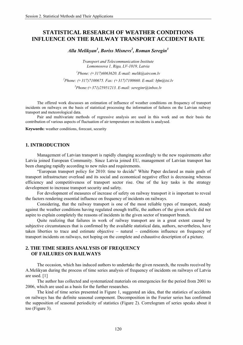
Session 2. Statistical Methods and Their Applications
120
STATISTICAL RESEARCH OF WEATHER CONDITIONS INFLUENCE ON THE RAILWAY TRANSPORT ACCIDENT RATE
Аlla Melikyan1, Boriss Misnevs2, Roman Seregin3
Transport and Telecommunication Institute
Lomonosova 1, Riga, LV-1019, Latvia 1Phone: (+317)6063620. E-mail: [email protected]
2Phone: (+317)7100675. Fax: (+317)7100660. E-mail: [email protected] 3Phone:(+371)25951213. E-mail: [email protected]
The offered work discusses an estimation of influence of weather conditions on frequency of transport incidents on railways on the basis of statistical processing the information of failures on the Latvian railway transport and meteorological data.
Pair and multivariate methods of regressive analysis are used in this work and on their basis the contribution of various aspects of fluctuation of air temperature on incidents is analysed.
Keywords: weather conditions, forecast, security 1. INTRODUCTION
Management of Latvian transport is rapidly changing accordingly to the new requirements after Latvia joined European Community. Since Latvia joined EU, management of Latvian transport has been changing rapidly according to new rules and requirements.
“European transport policy for 2010: time to decide” White Paper declared as main goals of transport infrastructure overload and its social and economical negative effect is decreasing whereas efficiency and competitiveness of transport sector rise. One of the key tasks is the strategy development to increase transport security and safety.
For development of measures of increase of safety on railway transport it is important to reveal the factors rendering essential influence on frequency of incidents on railways.
Considering, that the railway transport is one of the most reliable types of transport, steady against the weather conditions having regulated enough traffic, the authors of the given article did not aspire to explain completely the reasons of incidents in the given sector of transport branch.
Quite realizing that failures in work of railway transport are in a great extent caused by subjective circumstances that is confirmed by the available statistical data, authors, nevertheless, have taken liberties to trace and estimate objective – natural – conditions influence on frequency of transport incidents on railways, not hoping on the complete and exhaustive description of a picture. 2. THE TIME SERIES ANALYSIS OF FREQUENCY
OF FAILURES ON RAILWAYS
The occasion, which has induced authors to undertake the given research, the results received by A.Melikyan during the process of time series analysis of frequency of incidents on railways of Latvia are used. [1]
The author has collected and systematized materials on emergencies for the period from 2001 to 2006, which are used as a basis for the further researches.
The kind of time series presented in Figure 1, suggested an idea, that the statistics of accidents on railways has the definite seasonal component. Decomposition in the Fourier series has confirmed the supposition of seasonal periodicity of statistics (Figure 2). Correlogram of series speaks about it too (Figure 3).

The 7th International Conference “RELIABILITY and STATISTICS in TRANSPORTATION and COMMUNICATION - 2007”
121
Fig. 1. Time series of incidents on railways
Authors have pondered which factors characterize seasonal peculiarities. There is a large
number of such factors: temperature of air, a level of precipitation, a schedule of workers’ holidays on the railway... All of them are of interest from the point of view of studying statistics of transport incidents, but at the given research stage authors have concentrated attention to a temperature regime. The first natural assumption is the hypothesis about connection of accidents on railways with monthly average temperature. The regression constructed on data by quantity of transport incidents and monthly average temperature for 2005-2006, has indicated presence of connection between them (Figure 4).
It has turned out, that with downturn in temperature of air the probability of realization of transport incidents grows. Certainly, the temperature of air is not the main factor defining risk of occurrence of a non-staff situation on the railway, but all the same, this factor has the certain influence on frequency of incidents.
Fig. 2. Periodogram of time series of accidents

Session 2. Statistical Methods and Their Applications
122
Fig. 3. Correlogram of time series of accidents So, according to available data, correlation coefficient between frequency of accidents A and
monthly average temperature T equals ρ= -31 %, and at downturn of temperature on 10°С the average quantity of incidents on the Latvian railways increases on 9,1 %.
The standard mistake of coefficient b = -0,11 in the equation of regression equals eb=0,07 so the t-statistics is -1,54, what specifies that already significant at 14 % level the hypothesis about absence of connection between quantity of accidents and monthly average temperature rejects.
Fig. 4. Regression function of number of accidents on temperature
Thus, it is possible to draw a conclusion that winter is more dangerous season than summer in sense of accidents on railways.

The 7th International Conference “RELIABILITY and STATISTICS in TRANSPORTATION and COMMUNICATION - 2007”
123
3. AN ESTIMATION OF INFLUENCE OF TEMPERATURE FLUCTUATIONS ON ACCIDENTS
At the same time, it is represented quite probable, that not only value of temperature, but also its
fluctuation – especially sharp – can influence on accidents. For check of such hypothesis time series of daily increments of temperature has been
constructed and monthly average values of speed of its change are estimated.
30
1))(i(i)(30
2i∑=
−−=
TTTV . (1)
It has turned out, that the number of incidents on railways grows with growth of speed of
temperature change (Figure 5). Correlation coefficient between number of accidents A and average speed of change of
temperature TV equals ρ=26% the increment of average speed of daily fluctuations of temperature on 0,1°C leads to increase in accidents at 3,9 %.
Fig. 5. Regression function of number of accidents for speed of temperature change The standard mistake of coefficient b=3,54 in the equation of regression equals eb=2,84 so the
t-statistics is 1,25, i.e. significant at 22 % level the hypothesis about absence of connection between quantity of accidents and monthly average speed of temperature change rejects.
Thus, with a known degree of accuracy it is possible to say, that spring, accompanied rise in temperature is more dangerous season in sense of accidents than autumn.
At the same time with influence of change of temperature on accidents the question of temperature leaps influence on accidents has been studied. A time series of dependence of absolute value of daily fluctuations on air temperature has been constructed, monthly average value
30
|1)(i(i)|30
2i∑=
−−=
TTTVA (2)
are calculated and regression A on TVA is constructed. Results of these calculations are presented in Figure 6.

Session 2. Statistical Methods and Their Applications
124
Apparently, by growth of amplitude of temperature fluctuations the accidents increase. Correlation coefficient between number of accidents A and average amplitude of temperature fluctuations TVA equals ρ=23%, the increment of average amplitude of daily fluctuations of temperature on 1°C leads to increase in accidents at 11,6 %. The standard mistake of coefficient b=1,42 in the equation of regression equals eb=1,27 so the t-statistics is 1,11, i.e. significant at 28% level the hypothesis about absence of connection between quantity of accidents and monthly average amplitude of temperature fluctuations rejects.
Thus, time when sudden leaps of temperature are observed is more dangerous for accidents. Last conclusion is confirmed by one more calculation done within the limits of the present research. On the basis of statistical data for last years there is an estimation of normal daily temperature in Latvia N(t). Authors have constructed a time series of value of deviations of temperature of air from norm and investigated dependence of number of incidents on value of these deviations.
Fig. 6. Regression function of number of accidents on amplitude of temperature fluctuations
Fig. 7. Regression function of number of accidents on value of temperature deviation from norm
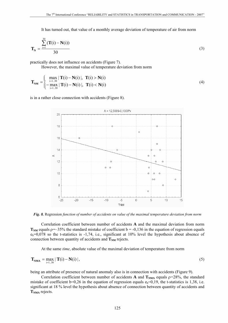
The 7th International Conference “RELIABILITY and STATISTICS in TRANSPORTATION and COMMUNICATION - 2007”
125
It has turned out, that value of a monthly average deviation of temperature of air from norm
30
(i))(i)(30
1i∑
=−
=NT
TN (3)
practically does not influence on accidents (Figure 7).
However, the maximal value of temperature deviation from norm
⎪⎩
⎪⎨⎧
<−−>−
==
=
)i()i(|,)i()i(|max)i()i(|,)i()i(|max
30..1i
30..1iNTNTNTNT
TNM (4)
is in a rather close connection with accidents (Figure 8).
Fig. 8. Regression function of number of accidents on value of the maximal temperature deviation from norm
Correlation coefficient between number of accidents A and the maximal deviation from norm TNM equals ρ=–35% the standard mistake of coefficient b = -0,136 in the equation of regression equals eb=0,078 so the t-statistics is -1,74, i.e., significant at 10% level the hypothesis about absence of connection between quantity of accidents and TNM rejects.
At the same time, absolute value of the maximal deviation of temperature from norm
|)i()i(|max
30..1iNTTNMA −=
=, (5)
being an attribute of presence of natural anomaly also is in connection with accidents (Figure 9).
Correlation coefficient between number of accidents A and TNMA equals ρ=28%, the standard mistake of coefficient b=0,26 in the equation of regression equals eb=0,19, the t-statistics is 1,38, i.e. significant at 18 % level the hypothesis about absence of connection between quantity of accidents and TNMA rejects.
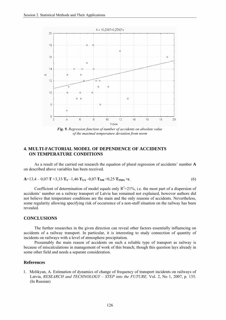
Session 2. Statistical Methods and Their Applications
126
Fig. 9. Regression function of number of accidents on absolute value of the maximal temperature deviation from norm
4. MULTI-FACTORIAL MODEL OF DEPENDENCE OF ACCIDENTS
ON TEMPERATURE CONDITIONS
As a result of the carried out research the equation of plural regression of accidents’ number A on described above variables has been received.
A=13,4 – 0,07⋅T +3,33⋅TV –1,46⋅TVA –0,07⋅TNM +0,25⋅TNMA +ε. (6)
Coefficient of determination of model equals only R2=21%, i.e. the most part of a dispersion of
accidents’ number on a railway transport of Latvia has remained not explained, however authors did not believe that temperature conditions are the main and the only reasons of accidents. Nevertheless, some regularity allowing specifying risk of occurrence of a non-staff situation on the railway has been revealed. CONCLUSIONS
The further researches in the given direction can reveal other factors essentially influencing on accidents of a railway transport. In particular, it is interesting to study connection of quantity of incidents on railways with a level of atmosphere precipitation.
Presumably the main reason of accidents on such a reliable type of transport as railway is because of miscalculations in management of work of this branch; though this question lays already in some other field and needs a separate consideration. References 1. Melikyan, A. Estimation of dynamics of change of frequency of transport incidents on railways of
Latvia, RESEARCH and TECHNOLOGY – STEP into the FUTURE, Vol. 2, No 1, 2007, p. 135. (In Russian)
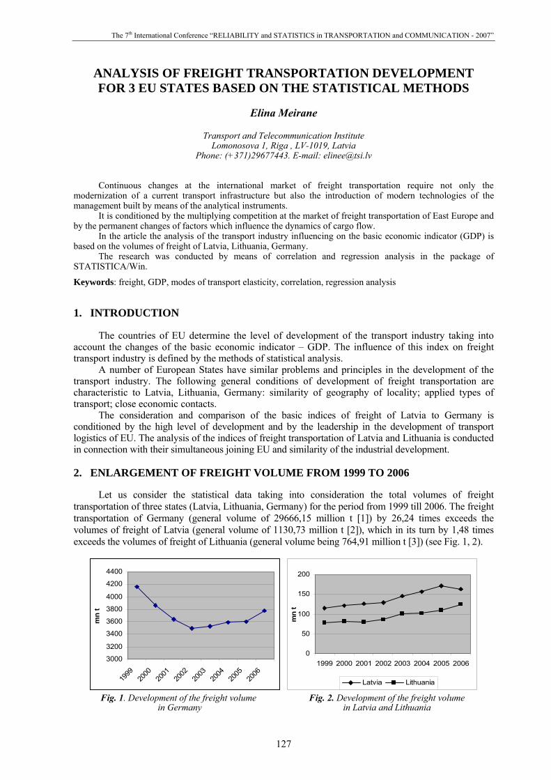
The 7th International Conference “RELIABILITY and STATISTICS in TRANSPORTATION and COMMUNICATION - 2007”
127
ANALYSIS OF FREIGHT TRANSPORTATION DEVELOPMENT FOR 3 EU STATES BASED ON THE STATISTICAL METHODS
Elina Meirane
Transport and Telecommunication Institute
Lomonosova 1, Riga , LV-1019, Latvia Phone: (+371)29677443. E-mail: [email protected]
Continuous changes at the international market of freight transportation require not only the modernization of a current transport infrastructure but also the introduction of modern technologies of the management built by means of the analytical instruments.
It is conditioned by the multiplying competition at the market of freight transportation of East Europe and by the permanent changes of factors which influence the dynamics of cargo flow.
In the article the analysis of the transport industry influencing on the basic economic indicator (GDP) is based on the volumes of freight of Latvia, Lithuania, Germany.
The research was conducted by means of correlation and regression analysis in the package of STATISTICA/Win.
Keywords: freight, GDP, modes of transport elasticity, correlation, regression analysis
1. INTRODUCTION
The countries of EU determine the level of development of the transport industry taking into
account the changes of the basic economic indicator – GDP. The influence of this index on freight transport industry is defined by the methods of statistical analysis.
A number of European States have similar problems and principles in the development of the transport industry. The following general conditions of development of freight transportation are characteristic to Latvia, Lithuania, Germany: similarity of geography of locality; applied types of transport; close economic contacts.
The consideration and comparison of the basic indices of freight of Latvia to Germany is conditioned by the high level of development and by the leadership in the development of transport logistics of EU. The analysis of the indices of freight transportation of Latvia and Lithuania is conducted in connection with their simultaneous joining EU and similarity of the industrial development.
2. ENLARGEMENT OF FREIGHT VOLUME FROM 1999 TO 2006
Let us consider the statistical data taking into consideration the total volumes of freight
transportation of three states (Latvia, Lithuania, Germany) for the period from 1999 till 2006. The freight transportation of Germany (general volume of 29666,15 million t [1]) by 26,24 times exceeds the volumes of freight of Latvia (general volume of 1130,73 million t [2]), which in its turn by 1,48 times exceeds the volumes of freight of Lithuania (general volume being 764,91 million t [3]) (see Fig. 1, 2).
3000
3200
3400
3600
3800
4000
4200
4400
1999
2000
2001
2002
2003
2004
2005
2006
mn
t
0
50
100
150
200
1999 2000 2001 2002 2003 2004 2005 2006
mn
t
Latvia Lithuania
Fig. 1. Development of the freight volume in Germany
Fig. 2. Development of the freight volume in Latvia and Lithuania

Session 2. Statistical Methods and Their Applications
128
For the analysed period (Latvia, Lithuania) the total volumes of freight transportation were increased by 40,46% and 57,18% accordingly, but in Germany the total volume of freight went down to 9,24%.
Determining the significance of the types of transport in distributing the freight flow of these states, the conclusions are drawn that in Germany the greater volume of cargo is on the road transport – 23291,3 million t, that constitutes 78,5% of the general volume. Concerning the other types of transport, the situation is as follows:
• rail – 2461,65 million t (8,3%), • maritime – 2031,1 million t (6,85%), • inland water – 1861,9 million t (6,28%), • air – 20,2 million t (0,07%) [1] (see Fig. 3).
In Latvia the biggest share of freight goes to the maritime transport – 441,64 million t, that constitutes 33,06% of the general volume, concerning the other types of transport, the real picture is:
• rail – 361,7 million t (31,99%), • road – 327,3 million t (28,94%), • air – 0,008 million t (0,007%) [2] (see Fig. 4).
In Lithuania the largest volumes go to the road transport - 400,61 million t from general volume, that constitutes 52,38% of the general volume, concerning the other types of transport, the situation is as follows:
• rail – 320,05 million t (41,84%), • maritime – 38,72 million t (5,06%), • inland water – 5,49 million t (0,72%), • air – 0,039 million t (0,005%) [3] (see Fig. 5).
0500
10001500200025003000350040004500
1999
2000
2001
2002
2003
2004
2005
2006
mn
t
Road Rail Maritime Air Inland w ater
020406080
100120140160180200
1999 2000 2001 2002 2003 2004 2005 2006
mn
t
Maritime Rail Air Road
Fig. 3. Development of the freight volume in Germany from 1999 to 2006
Fig. 4. Development of the freight volume in Latvia from 1999 to 2006
0
20
40
60
80
100
120
140
1999 2000 2001 2002 2003 2004 2005 2006
mn
t
Rail Road Maritime Inland w ater Air
Fig. 5. Development of the freight volume in Lithuania from 1999 to 2006

The 7th International Conference “RELIABILITY and STATISTICS in TRANSPORTATION and COMMUNICATION - 2007”
129
The freight volumes for these states for 2006 in percents according to the modes of transport are distributed as it is shown in Fig. 6-8.
9,08%
76,52%
6,35%0,08%7,97%
Rail Road Maritime Air Inland w ater
30,00%0,02%
36,63%33,36%
Maritime Rail Air Road
Fig. 6. Distribution of the freight volume by modes of transport in Germany in 2006
Fig. 7. Distribution of the freight volume by modes of transport in Latvia in 2006
45,76%
48,96%
4,66%0,62%
0,01%
Rail Road Maritime Inland w ater Air
Fig. 8. Distribution of the freight volume by modes of transport in Lithuania in 2006
Having compared the distribution of volumes of freight according to the different types of
transport for the whole examined period (1999-2006) we drew the following conclusions: • invariability of the leading types of transport; • redistribution of traffic of cargo on the types of transport only in Latvia; • decline of the share of freight on the road transport in Germany (-1,98%),
on the railway of transport in Latvia (-1,99%), road (-3,42%), maritime (-0,4%) and inland water (-0,1%) in Lithuania.
Table 1. Distribution of volumes of freight (%)
Modes Time Period
Road Rail Maritime Inland water
Air
1999-2005, (%) 78,5 8,3 6,85 6,28 0,07 2006 (%) 76,52 9,08 7,97 6,35 0,08 Germany Difference (%) -1,98 0,78 1,12 0,07 0,01 1999-2005, (%) 28,94 31,99 33,06 - 0,007 2006 (%) 33,36 30,00 36,63 - 0,02 Latvia Difference (%) 4,42 -1,99 3,57 - 0,013 1999-2005, (%) 52,38 41,84 5,06 0,72 0,005 2006 (%) 48,96 45,76 4,66 0,62 0,01 Lithuania Difference (%) -3,42 3,92 -0,4 -0,1 0,005

Session 2. Statistical Methods and Their Applications
130
The further analysis of volumes of the transported cargo and types of transport of the examined states showed that the most significant types of transport for Latvia are the following: Maritime, Rail and Road.
3. FREIGHT ELASTICITY
The analysis of the freight will be conducted by means of the method presented in the report on a project Scenes [4]. According to this method it is necessary to take into account the following calculations: "decoupling" is dealt with the present study focusing on the analysis of the growth rates of GDP and growth rates of indicators describing freight transport demand (transport volume). Thus decoupling of the evolution of transport demand from the evolution of GDP has taken place, the transport demand and growth path being with lower growth rates than GDP.
Comparing the growth of GDP to the growth of changes of demand for the freight transport, we could calculate the transport elasticity by means of the formula [4]:
2)(
2)(
,,,
ba
ba
ba
baYba GDPGDP
GDPYY
Y+
Δ÷
+Δ
=η ,
where
−η transport elasticity, −Y transport demand indicator (transport volume) in million t,
−GDP the Gross Domestic Product at current prices in million t [2], [5], [6], −ba, period of time η refers to (period of time between year a and year b).
Table 2. Transport elasticity by modes
Transport elasticity η referring to transport volume by modes
Period of time Total Rail Road Maritime
1999-2006 -0,709 1,289 -1,240 2,365 1999-2003 -2,276 1,328 -3,082 2,038 2000-2004 -1,047 1,652 -1,721 2,391 2001-2005 -0,170 1,637 -0,636 2,526
Germany
2002-2006 1,043 1,798 0,820 2,912 1999-2006 0,559 0,841 0,359 0,376 1999-2003 0,520 0,901 0,286 0,178 2000-2004 0,611 1,026 0,352 0,120 2001-2005 0,791 1,239 0,494 0,498
Lithuania
2002-2006 0,783 0,961 0,663 2,426 1999-2006 0,346 0,389 0,488 0,198 1999-2003 0,476 0,805 0,460 0,227 2000-2004 0,593 0,959 0,667 0,231 2001-2005 0,487 0,740 0,749 0,087
Latvia
2002-2006 0,309 0,263 0,514 0,178
In Table 2 the coefficients of elasticity are reflected for the whole analysed period (1999-2006) and for the periods of five years.
The coefficients of freight volumes general elasticity of the three states (with Germany of 2002-2006 as an exception) being less than 1, it shows that for the period from 1999 till 2006 the transport industry of these states had not used the general potential of development, as an economy of the states had more considerable growth as compared to the growth of the freight transport volume. More stable values have the coefficients of general elasticity below 1 in Latvia and
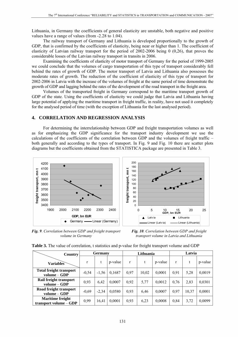
The 7th International Conference “RELIABILITY and STATISTICS in TRANSPORTATION and COMMUNICATION - 2007”
131
Lithuania, in Germany the coefficients of general elasticity are unstable, both negative and positive values have a range of values (from -2.28 to 1.04).
The railway transport of Germany and Lithuania is developed proportionally to the growth of GDP, that is confirmed by the coefficients of elasticity, being near or higher than 1. The coefficient of elasticity of Latvian railway transport for the period of 2002-2006 being 0 (0,26), that proves the considerable losses of the Latvian railway transport in transits in 2006.
Examining the coefficients of elasticity of motor transport of Germany for the period of 1999-2005 we could conclude that the volumes of cargo transportation of this type of transport considerably fell behind the rates of growth of GDP. The motor transport of Latvia and Lithuania also possesses the moderate rates of growth. The reduction of the coefficient of elasticity of this type of transport for 2002-2006 in Latvia with the increase of the volumes of freight at the same period of time demonstrate the growth of GDP and lagging behind the rates of the development of the road transport in the freight area.
Volumes of the transported freight in Germany correspond to the maritime transport growth of GDP of the state. Using the coefficients of elasticity we could judge that Latvia and Lithuania having large potential of applying the maritime transport in freight traffic, in reality, have not used it completely for the analysed period of time (with the exception of Lithuania for the last analysed period).
4. CORRELATION AND REGRESSION ANALYSIS
For determining the interrelationship between GDP and freight transportation volumes as well as for emphasizing the GDP significance for the transport industry development we use the calculations of the coefficients of the correlation between GDP and the volumes of freight traffic – both generally and according to the types of transport. In Fig. 9 and Fig. 10 there are scatter plots diagrams but the coefficients obtained from the STATISTICA package are presented in Table 3.
340035003600370038003900400041004200
1900 2000 2100 2200 2300 2400
GDP, bn EUR
frei
ght t
rans
port
, mn
t
Germany Linear (Germany)
02040
6080
100120140160180200
0 5 10 15 20 25GDP, bn EUR
frei
ght t
rans
port
, mn
t
Latv ia Lithuania
Linear (Latv ia) Linear (Lithuania)
Fig. 9. Correlation between GDP and freight transport volume in Germany
Fig. 10. Correlation between GDP and freight transport volume in Latvia and Lithuania
Table 3. The value of correlation, t statistics and p-value for freight transport volume and GDP
Germany Lithuania Latvia Country
Variables r t p-value r t p-value r t p-value
Total freight transport volume – GDP -0,54 -1,56 0,1687 0,97 10,02 0,0001 0,91 5,28 0,0019
Rail freight transport volume – GDP 0,93 6,42 0,0007 0,92 5,77 0,0012 0,76 2,83 0,0301
Road freight transport volume – GDP -0,69 -2,34 0,0580 0,93 6,46 0,0007 0,97 10,37 0,0001
Maritime freight transport volume – GDP 0,99 16,41 0,0001 0,93 6,23 0,0008 0,84 3,72 0,0099

Session 2. Statistical Methods and Their Applications
132
As it is shown in Table 3, not all the values of t statistics are significant (p-value < 0,05). For example, the values of t statistics (and accordingly p-value) at the analysis of correlation between Total freight volume and GDP for Germany are not significant. It shows that the transport industry of Germany has not large influence on forming the GDP. The significant development of the transport complex leads to this result. The Eurostat Statistical Bureau presents the data proving that in Germany GDP per capita in 2006 constituted 113% of the average level of ЕU countries.
As the elasticity and correlation coefficient shows only the presence or absence of the dependence between the analysed variables, but does not give the whole picture of their linking, it is useful to build the regression model [4], [7]:
iii uXbbY ++= 21 ,
where −Y freight transport volume at the i moment of time in million t, −X value GDP at the i moment of time in million t,
−21 ,bb the parameters of the regression line.
The results of the regression line estimation by the least-squares method are shown in Table 4.
Table 4. Equations for regression lines
Regression lines
Total transport
volume Road transport
volume Rail transport
volume Maritime
transport volume
Germany =6363,9043-0,00123*GDP
=6683,2456-0,00175*GDP
= -116,1963+ 0,0002*GDP
= -366,5832+ 0,00029*GDP
Lithuania =36,6564+ 0,00367*GDP
=29,8774+ 0,00124*GDP
=9,8737+ 0,00198*GDP
=3,2439+ 0,0001*GDP
Latvia =91,6327+ 0,00535*GDP
=19,1307+ 0,00234*GDP
=25,9118+ 0,00208*GDP
=46,5979+ 0,00093*GDP
Before using these models for the analysis of he influence of variable – GDP on freight volume,
it is necessary to consider the model quality (see Table 5.).
Table 5. Quality analysis of obtained regression equations
F (1,6) p-level SEE Durbin-Watson (d) Total freight 0,290 2,448 0,169 199,510 0,745 Rail freight 0,873 41,178 0,001 7,765 1,824 Road freight 0,477 5,468 0,058 189,600 0,735 Germany
Maritime freight 0,978 269,250 0,000 4,445 1,007 Total freight 0,944 100,320 0,000 4,271 1,610 Rail freight 0,847 33,276 0,001 4,040 3,019 Road freight 0,874 41,689 0,001 2,270 1,813 Lithuania
Maritime freight 0,931 38,754 0,001 0,186 1,138 Total freight 0,823 27,877 0,002 9,514 1,429 Rail freight 0,571 7,987 0,030 6,902 1,279 Road freight 0,947 107,623 0,000 2,122 1,844
Latvia
Maritime freight 0,697 13,828 0,010 2,339 2,138
−2R coefficient of determination. If the value is close to 1, it means the good quality of model.
2R

The 7th International Conference “RELIABILITY and STATISTICS in TRANSPORTATION and COMMUNICATION - 2007”
133
F (1,6) are F-statistics for testing the hypothesis about regression nonsignificant, at the level of significance 5% – the critical value is 95.0F (1,6) = 5,99.
SEE is a standard error of regression, used as a basic measure of the quality estimated model. Durbin-Watson (d) is the statistics for testing the hypothesis about absence of autocorrelation [7]. In Table 5 the quality criteria of values of the significant models are emphasized. On the basis of
the conducted analysis of quality there are built the regression equations and it is possible to draw the following conclusions:
• only two of the built models (Germany – Rail freight and Germany – Maritime freight) cannot be used for the analysis, because the regression is insignificant;
• at increasing GDP by 1 billion EUR the general traffic of cargo of Latvia and Lithuania will be multiplied by 5,35 million t and by 3,63 million t accordingly, the coefficient of GDP will show the number of times by which the GDP coefficient will be increased.
CONCLUSIONS
The conducted analysis of the development of freight transport in the considered countries confirms once again the close interconnection between the level of the development of GDP and freight industry of the new members of EU. The calculations made by means of the statistical methods demonstrated that the developing transport industry considerably influences the GDP formation, especially in the states of the Baltic Region.
The analysis of elasticity shows that for the period from 1999 till 2006 the transport industry of Latvia and Lithuania did not use the general potential of the development, as an economy of the states had the pre-potential growth as compared to the growth of the freight transport volume.
The invariability of priorities is certain in distributing the freight flow according to the modes of transport during the examined period (in Latvia – the maritime transport, in Lithuania – the road transport, in Germany – the road transport). The different geographical peculiarities of the Baltic countries influence the choice of the popular modes of transport for every country (Latvia, Germany, Lithuania).
The analysis of the freight volume in Latvia according to the modes of transport for the period from 1999 till 2006 indicates that it is necessary to pay attention to the multimodal transportation, namely, to three basic modes of transport (Fig.7). In this connection the great attention is focused on the close links between maritime, railroad and road transport in Latvia. References 1. Passengers carried/goods carried – http://www.destatis.de/basis/e/verk/verktab5.htm (25.05.07.) 2. Central Statistical Bureau of the Republic of Latvia. Transport in 2006: the collection of statistical
data. Riga, 2007. (In Latvian) – (http: //www.csb.gov.lv) 3. Krovinių vežimas – http://www.stat.gov.lt/lt/pages/view/?id=1228&PHPSESSID=e420e5a11a2be8
bec5974ee4eb99e38 (25.05.07.) 4. SCENES Deliverable D3a –List of Appendix Documents. Drivers of Transport Demand – Western
European Countries - Contract No ST-97-RS.2277, 28 April 2000. 5. Verwendung des Bruttoinlandsprodukts Deutschland in jeweiligen Preisen Mrd. EUR –
http://www.destatis.de/jetspeed/portal/cms/Sites/destatis/Internet/DE/Content/Statistiken/Zeitreihen/LangeReihen/VolkswirtschaftlicheGesamtrechnungen/Content100/lrvgr02a,templateId=renderPrint.psml (25.05.07.)
6. Gross Domestic Product – http://www.stat.gov.lt/uploads/docs/BVP_2007_1Q_30.xls (25.05.07.) 7. Dowgerty, K. Introduction to Econometrics, 2nd ed. Moscow: INFRA-M, 2004. (In Russian)

Session 2. Statistical Methods and Their Applications
134
STATISTICAL ANALYSIS OF AERONAUTICAL INFORMATION SYSTEM WITH OBJECTIVE TARGET FOR PROSPECTIVE
OPERATIONS
Jörg Kundler
PhD Student, Transport and Telecommunications Institute, Riga, Latvia Head of IT-Services, DFS, Deutsche Flugsicherung GmbH, Langen
Am DFS-Campus 7, D-63225 Langen Phone: (+49)61037072530. Fax: (+49)61037074596. E-mail: [email protected]
The AIS service (Aeronautical Information Service) is an operational service for Air Traffic Control and the functionality via availability and data integrity is one of the critical factors for the AIS Centre. Particularly the AIS Service is highly dependent on IT-Systems, technical infrastructure and their availability. The investigation shows the relevant standard requirements of availability and long-term maintenance to an AIS-System and their statistical analysis.
The goal of statistical analysis is to investigate the observed parameter like availability and robustness of functionality and services and to derive technical expertise for a migration project of
AIS Services to a new IT-platform and bring in a new concept for technical operation. For that reason the figure presents the number and distribution of different incident types over the observed operational period. The definition of incident types is clarified with the operational customer. Main criteria of incidents are the differentiation between failure and coordinated maintenance incidents and the related impact of the aeronautical operation. In the plot is visible that all kind of plots are flatter and not homogenously, all types contain a different level of extremes. The failures of incident category t>20 minutes which have direct impact to the operation are only singular and have a nearly homogenously distribution over the complete operational period.
In the paper research of maintenance parameter based on the statistical analysis, and results for further operational use are discussed. The statistical analysis will be used for project planning process of a migration on new system technology in parallel to the normal operational use at end of actual used system life cycle in year 2009. Especially the statistical investigation will be used for detecting of lacks in operation and maintenance process, defects of hardware, operational system, data base and application. The analysis of different incident types and their characteristics based on the collected statistical maintenance data over operational period from 2001 to 2006 is performed. The results of statistical investigation will be also used for a more stabile forecasting of operational use and get statistical information for the future trend of ATC System and their real availability parameter. The statistical analysis has shown the relevant requirements of ATC maintenance for long-term use of IT Systems.
Keywords: long-term life cycle, maintenance and reliability of ATC systems, research of incident characteristics, statistical expertise for migration 1. INTRODUCTION
The integrated AIS System is responsible for the technical provision of aeronautical briefing information. This system includes a world-wide data base with all necessary technical and organizational information for world wide flights. The main requirements are to assure a high availability of function and complete data integrity of data base. This system has the status of legal ATC operational system. The operational time of system is 24 hours and 365 days.
The integrated AIS system is being in operational use since year 2000 in a computer centre on Frankfurt Airport. The planned life cycle of this system should be finished until the end of 2009. Due to different reasons the life cycle of operation shall to extent until year 2011. The goal of research is the statistical analysis of operational data for forecasting of such an opportunity. Software Statistica Release 6 was used for investigation. 2. DESCRIPTION AND ANALYSIS OF INPUT DATA BASE
The statistical input data base contains all technical failures during the operational time period from January 2001 until April 2006. The data base contains the following information: date and time of failure, time period of failure, related failure system / part of system, short description of failure
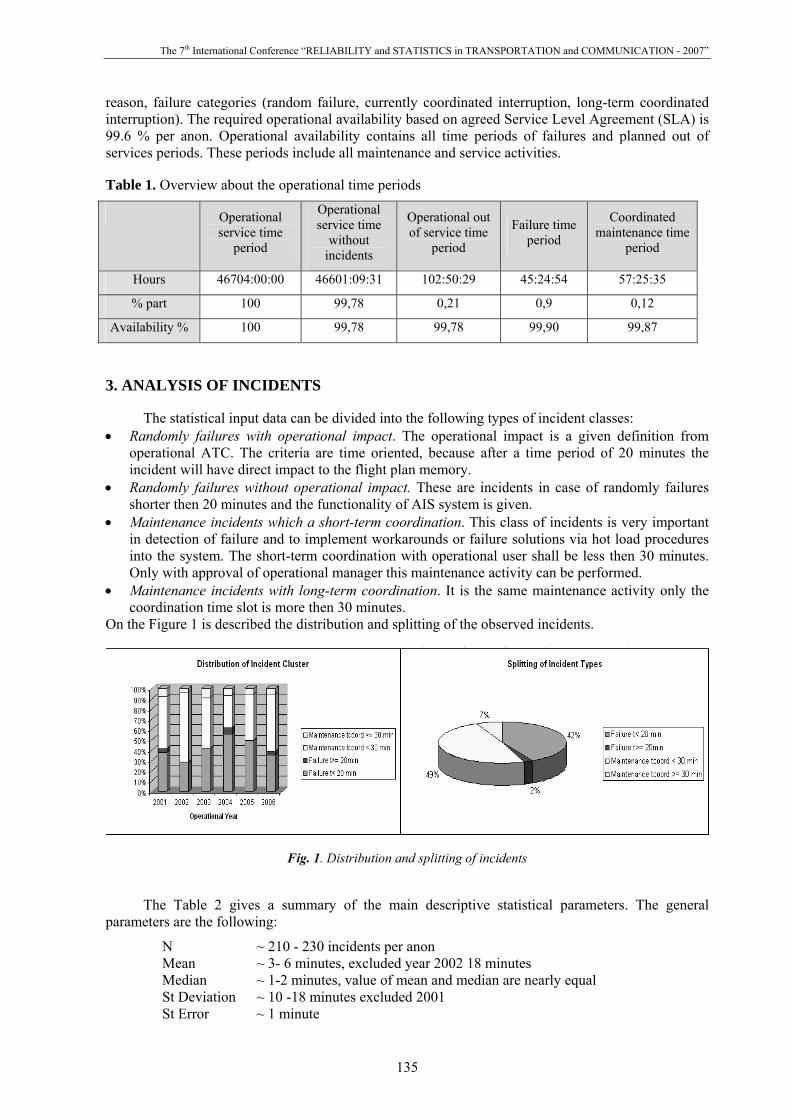
The 7th International Conference “RELIABILITY and STATISTICS in TRANSPORTATION and COMMUNICATION - 2007”
135
reason, failure categories (random failure, currently coordinated interruption, long-term coordinated interruption). The required operational availability based on agreed Service Level Agreement (SLA) is 99.6 % per anon. Operational availability contains all time periods of failures and planned out of services periods. These periods include all maintenance and service activities. Table 1. Overview about the operational time periods
Operational service time
period
Operational service time
without incidents
Operational out of service time
period
Failure time period
Coordinated maintenance time
period
Hours 46704:00:00 46601:09:31 102:50:29 45:24:54 57:25:35
% part 100 99,78 0,21 0,9 0,12
Availability % 100 99,78 99,78 99,90 99,87
3. ANALYSIS OF INCIDENTS
The statistical input data can be divided into the following types of incident classes: • Randomly failures with operational impact. The operational impact is a given definition from
operational ATC. The criteria are time oriented, because after a time period of 20 minutes the incident will have direct impact to the flight plan memory.
• Randomly failures without operational impact. These are incidents in case of randomly failures shorter then 20 minutes and the functionality of AIS system is given.
• Maintenance incidents which a short-term coordination. This class of incidents is very important in detection of failure and to implement workarounds or failure solutions via hot load procedures into the system. The short-term coordination with operational user shall be less then 30 minutes. Only with approval of operational manager this maintenance activity can be performed.
• Maintenance incidents with long-term coordination. It is the same maintenance activity only the coordination time slot is more then 30 minutes.
On the Figure 1 is described the distribution and splitting of the observed incidents.
Fig. 1. Distribution and splitting of incidents
The Table 2 gives a summary of the main descriptive statistical parameters. The general parameters are the following:
N ~ 210 - 230 incidents per anon Mean ~ 3- 6 minutes, excluded year 2002 18 minutes Median ~ 1-2 minutes, value of mean and median are nearly equal St Deviation ~ 10 -18 minutes excluded 2001 St Error ~ 1 minute

Session 2. Statistical Methods and Their Applications
136
Findings of the statistical analysis of incident distribution are as follows: • The distribution of random sample is homogenous. • The reason for high values of standard deviation and standard error reflects that the incident clustering
is not performed by a scientific statistical methods like cluster analysis and is not calculated by different similarity or distance coefficients like Minowski distance or Euclidian distance.
• The clustering of different types of incidents is given by practical reason and operational business need. So the calculated parameter can be different from the scientific border.
• Over the operational period it shall be expected around 200 incidents per anon, but only 2% of them have operational impact of the AIS functionality.
• The availability of the service is higher than the required one. But over the operational time period it is not visible that the system will reach more robustness and stability.
• The distribution of different kind of incidents is shown by the following Box & Whisker Plot. We can see the correlation between the different types of incidents. In general the types Failures t<20 minutes and maintenance t >= 30 minutes are very similar, also the other two kinds of incidents are similar from the descriptive statistical parameters.
• The mean value for incidents with operational impact is 00:51:09 minutes. The median value is 00:53:48 minutes. The mean and median values are very similar.
• Mentionable is that 95% confidence interval is 00:32:10 / 01:10:08. The most part of problems are solved by changes or workaround inside of 01:10:08 minutes. Long-term down time period is not detected.
• For incidents t<20 minutes the time period between min and max is from 14 sec. to 17 min., the value of standard deviation is really small. The time span is delimited by maximum 20 minutes.
• The arithmetic mean (00:02:13) and the median (00:01:40) differ around 25 %. • The most number of incident plots by 95% confidence interval is related between 00:01:51 and
00:02:34. • The distribution of incident plots is not so homogenous like the incidents of category t>20 minutes. Table 3. Calculation of basic descriptive statistical characteristics by Statistica6
Fig. 2. Box & Whisker Plot of incident types
Box & Whisker Plot
Num
ber o
f Inc
iden
ts
Failu
re t
< 20
min
Failu
re t>
20 m
in
Mai
nten
ance
tco
ord
<30
min
Mai
nten
ance
tco
ord
>=30
min
-500
50100150200250300350400
Num
ber o
f Inc
iden
ts
Mean ±SD ±1,96*SD

The 7th International Conference “RELIABILITY and STATISTICS in TRANSPORTATION and COMMUNICATION - 2007”
137
Fig. 3. Time series of all kinds of incidents types per operational month
With reference to the analysis the following pattern can be observed: • After 7-8 month of operation the number of incidents decreases in a strong way. The next
operational year of AIS-system was performed on the similar level of incident number until April 2005.
• The number of incidents in April 2005 is extremely escalated, because during this period the AIS System is updated and changed by a high number of changes requests. After realization of these large system changes the use of system shall be established in more robustness and more stabile, because on the Figure 3 is visible that the number of incidents in general is decreased.
• Based on a 6-7 years used hardware platform the number of incidents is not increased. • All kind of plots are flatter and not homogenous, all types contain a different level of extremes. In
the plot is visible that the failures of incident category t>20 minutes which have direct impact to the operation are only singular and have a similar homogenous distribution over the complete operational period.
• The extremely outlier is the high number of maintenance incidents t>30 minutes during August and September 2003. Also during this time period we can observe a high number failures t<20 minutes and maintenance incident t<30 minutes. This is a strong indication of instable system operation and strong impact of changes to the system availability and robustness. The same pattern can be observed during the time period on April 2005.
4. FINDINGS OF STATISTICAL ANALYSIS
The statistical analysis gives the scientific approval of the following findings and conclusions: • Based on the actual system the availability of AIS service and functionality is fulfilled and meets
the requirements. • From investigation point of view the required SLA parameter „Availability” is not sufficient and
not complains for a complete description of service quality and statistical analysis. • In addition it will be necessary to define new parameter like stability and robustness. From the
SLA point of view it shall be agreed also a max time period out of service is dependent on failure or maintenance category, because from the customer’s point of view only the functionality of service is important. The reasons of activities are in responsibility of service provider.
• Additionally also a maximal number of incidents per anon or per month shall be defined.

Session 2. Statistical Methods and Their Applications
138
• From statistical point of view it is visible that the number of incidents over operational years is stabile.
• It is not recognizable that by the long operational use of the systems and in particular the hardware platform an increase of incidents is visible.
• It is also not evident that the system and service is vulnerable by regular bringing in of new functionality, updates, patches and the system design is vulnerable to changes.
• With respect to the system migration in 2009 on a new system platform is very important to perform a migration to a more stabile and robust operational system.
• For increasing operational cost and to have an independent system platform is making sense to work out a new design. To design the system in that way, that exists an independent IT system platform with an independent operational system, preferable an open source operational system like LINUX and to have an independent hardware platform. In addition the AIS application can to bring into a virtualised system platform.
5. DERIVATIONS FOR SYSTEM MIGRATION AND OPERATION CONCEPT
Based on the statistical findings, especially the reached high availability, reliability and extremely small number of incidents with operational impact gives the possibility to optimise the system architecture with respect to decrease the maintenance cost.
The system architecture of AIS-System is to redesign during operational use from an operational production system with 6 different replicas to a system structure with a production system with 3 replicas. The different data bases located on different replicas are consolidated to a data base on 3 replicas. These replicas contain the data base for the AIS-Centre; merge data base and one space replica.
The continuity concept is also adapted. The main concept is changed from a 4-System-Concept to a 3-System-Concept with a separate Production-Reference-Test-System. The Test and Continuity Systems are consolidated.
Based on this optimisation it is possible to decrease the cost for hardware and also cost for software maintenance and at the same time to assure the required SLA availability parameter.
In addition based on new customer requirements the AIS-System is expanded to new functionalities like FAX and e-mail server for aeronautical briefing via Internet and a new data robot and media server for data recovery.
With the approval of statistical analysis the architecture of AIS-System is consolidated and the system complexity is decreased. The benefit is the decreasing of maintenance cost and guarantee of same service quality, but with increasing service quantity of AIS-System.
Taking into account for the planned relocation of AIS-System the following main topics for a new possible operation and migration concept are developed: • Technical integration into the central computer centre and existing IT-Infrastructure, Maintenance
Concept and Service Processes • Joint use of IT-Basic Infrastructure like Data Robot and Data Recovery • Joint use of IT-Basic Services like common use of resources for hardware maintenance and
maintenance contracts with service providers • Change the IT-Business Technology from IT-Support by systems (Functionality, Application,
System Infrastructure) to IT-Services • IT-Services mean providing of services of application level and functionality level by using of a
common IT-Landscape and Infrastructure, by using of common resources for It-infrastructure • Starting of implementation of Service Oriented Architecture (SOA) Technology and
differentiation between a general virtual IT-Basic Infrastructure which can be used by different applications together
• Increasing the standardization level of system management working position (Service Level 1) • Increasing the automation level of system monitoring and management based on automated
system and service management tools which are combined with the work flow processing.
The investigation has also positive impact and approval for development of a relocation concept of AIS-System with minimum operational impact and changing the communication infrastructure in parallel. The relocation concept contains the following main steps.

The 7th International Conference “RELIABILITY and STATISTICS in TRANSPORTATION and COMMUNICATION - 2007”
139
1. Migration of Test Systems on new communication infrastructure 2. Test and Approval Sessions of these systems and system freeze 3. Switch off old production systems and relocation to the new computer centre 4. Migration of systems on new location into the new IT-infrastructure and communication
infrastructure 5. Test and Approval sessions and switch to the new production system on new location of
service management centre 6. Switch of the production systems on old location and relocation to the central test centre
and build up to the test system level.
Due to the fact that the AIS System is a legal operational ATC-Service the test and approval scenarios have to include the following main test cases:
Daily Data Input Test Check Housekeeping and Backup System Operation Tests
- Recovery and Alarm Handling - Backup Procedure Test
Hot Load Testing - Master and Production System - Data Base and Replicas
System Recovery Test - Switch Production, Redundancy and Replicas - Input Messaging Test - Stress and Overload Test - Recovery Test for Data Lost and Damages
Messaging Handling Test - AFTN Messaging - Netware Test - Manual Messaging - Automatically Messaging
The statistical analysis delivers important information about the system’s behaviours and has a direct impact of the conceptual development to relocation plan and testing concept. Basic principles for analysis are the permanent and long-term collection of statistical data and their analysis via system management tool. Based on significant statistical data base it is possible the derived forecasting information of system availability and lacks of software processes. The analysis can be helpful and it delivers a valuable input of possible projects, like migration of a new IT or Communication infrastructure or relocation of a complete computer centre.
References 1. Rinne, H. Statistische Analyse multivatianter Daten. R. München: Oldenbourg Verlag München. 2. Yatskiv, I. Multivariate Statistical Analysis: classification and dimension reduction. Riga: Transport
and Telecommunications Institute, 2003. (In Russian) 3. Backhaus, Erichson, Plinke, Weiber. Multivariante Analysemethoden, Eine anwendungsorientierte
Einführung. Springer Verlag, 1994. 4. Kreyzig, E. Statistische Methoden und ihre Anwendungen. Göttingen: Vandenhoeck&Ruprecht
Verlag, 1975. 5. Statistical Software Program Statistica 6, including Handbook. 6. Interview with Mr. Norbert Konle Manger about Flight Data Management Processing.
Session 2. Statistical Methods and Their Applications
140
THE ECONOMETRIC ANALYSIS OF INVESTMENT STRUCTURE MODEL
Deniss Titarenko
Transport and Telecommunication Institute
Lomonosova 1, Riga, LV-1019, Latvia Phone: (+371)67100573. E-mail: [email protected]
The aim of the paper is to estimate the influence of different structural elements of investment on the economic growth in Latvia. Author presents the brief review of the main development trends of the modern economic growth theory. The dynamics and structure of the nonfinancial investment of the Latvian enterprises is analysed. The results of econometric analysis of the investment structure model presented in this paper show that intangible investment, investment in nonresidential buildings and machinery investment are the most significant factors influencing the level of labour productivity in Latvia.
Keywords: nonfinancial investment, investment structure, labour productivity 1. THE ROLE OF INVESTMENT FACTOR IN MODERN ECONOMIC
GROWTH THEORY Research in modern economic growth theory is closely related to the empiric analysis which
gives the opportunity to verify and substantiate or refute theoretical conclusions. According to the Neoclassical approach the economic growth is defined as exogenous process
because its technological parameters are not dependent on defined parameters such as capital and labour. The early neoclassical growth models were based on well-known Cobb-Douglas production function introduced by Charles W. Cobb and Paul H. Douglas in 1928. The Cobb-Douglas production function is widely used to represent the relationship of an output to inputs (formula 1) [1, 61]:
Y = f(K,L) , (1) where Y – output, K – capital, L – labour.
Let us suppose that output elasticity with respect to labour and capital is denoted by α and β respectively, where a + β = 1. So the Cobb-Douglas production function normally has the form akin to the following [1, 61]:
Y = A×KαLβ , (2)
where A – proportion coefficient determined by the technological progress. The values of all three parameters in formula 2 – A, α and β are unknown and should be
determined by analysing the empirical statistical data. The value parameter α always ranges from 0 to 1. If α tends to zero, it implies decreasing return of capital. And vice versa – if α tends to 1, the return of capital is growing.
The rising popularity of empiric analysis driven by the development of its methodology in the second half of the 20th century has highlighted many questions which could not be settled under the basic Neoclassical theory. The results of empiric analysis gave the evidence of significant shift from the conceptual framework of Neoclassical theory which was stated by D. Cass, T.C. Koopmans, P.A. Diamond, N. Kaldor and other economists. Empirics show that in long-term the convergence of economic development level of different countries does not really exist and the typology of economy growth behaviour all over the world is much wider than it is proposed by Neoclassical theory. It means that in modern conditions the interpretation of economic growth process based only on two main factors – i.e. capital and labour (see formula 1) – is out of date. So the necessity to involve into analysis much wider set of growth determinants has become the incentive for the development of new endogenous theory of economic growth in the 1980`s.

The 7th International Conference “RELIABILITY and STATISTICS in TRANSPORTATION and COMMUNICATION - 2007”
141
Summary of the results of modern empiric research of economic growth process could be found in the World Bank working paper prepared by W.Easterly and R.Levine (Easterly, Levine, 2000). The authors propose the following 5 stylised facts:
1. Factor accumulation does not account for the bulk of cross-cross differences in the level or growth rate of GDP per capita; something else – total factor productivity (TFP) – accounts for a substantial amount of cross-country differences.
2. Divergence: there are huge, growing differences in GDP per capita. 3. Growth is not persistent over time. Some countries “take off,” others are subjected to peaks
and valleys, a few grow steadily, and others have never grown. In contrast, capital accumulation is much more persistent than overall growth.
4. All factors of production flow to the same places, suggesting important externalities. 5. National policies influence long-run growth [2, 21]. So it is possible to conclude that economic growth process can not be explained only by
accumulation and movement of the major production factors (capital and labour). It is necessary to search for other determinants of growth which are usually "hidden" in the residual member of the production function. Exactly the determinants of the total factor productivity in the modern conditions are the most substantial explanatory variables of the economic growth process. These variables – subjective behavioural and institutional factors – determine the sustainable economic growth of each country.
Usually the most part of the empiric research models of growth determinants is based on standard type of the growth equation which contains traditional economic variables (investment, capital, labour and others) together with additional potentially statistically significant determinants. The basic regression equation can be presented as follows [3, 22]:
∑∑∑ ++++=r
irirp
pipe
eiei DUMczbxaag ε0 , (3)
where ig – growth rate of the gross national product indicators (GDP, GNP) in country i; 0a – constant; ea – coefficient of an economic variable; eix – economic variables; pb – coefficients of the
additional variables; piz – additional variables (political, social, demographic and others); rc – coefficient of the dummy variable; riDUM – dummy variable which defines the group effect (for example, regional effect and so on); iε – random error.
Upon the whole, it should be noted that in the 1990s and in the beginning of the 21st century a great number of different research papers and studies were made for evaluation of considerably wide range of new determinants (political, social, demographic, ethnic, religious and others) of economic growth. For example, well-known economist Xavier X. Sala-i-Martin in 1997 has published a paper which presents the analysis of an influence of 62 different factors on economic growth process as the result of evaluation of approximately two million regressions (Sala-i-Martin, 1997).
The significant place among other growth determinants belongs to the parameters of investment processes. There are many research papers which are devoted to the analysis of the interrelations between such investment parameters as investment norm (the share of investment in GDP) or type of investment (equipment (machinery) investment, other (non-equipment) investment) and economic growth. Table 1 presents the summary of major results of the evaluation of investment determinants of economic growth.
As it is mentioned above, the aim of this paper is to estimate the influence of different structural elements of investment on the process of economic growth. It should be noted here that the economists and chronologists of economic thought avow that in long run the rapid economic growth is not possible without any significant investments into the corporate capital funds. It is no accident that the era in which European economic growth took off is called the Industrial Revolution. The French politician Blanqui (1837) identified its beginnings in the invention and spread of those “two machines, henceforth immortal, the steam engine and the cotton spinning (frame).” Ever since, qualitative historical discussions of growth have emphasized the role of investment in machinery in augmenting labour power. Landes’ (1969) statement that “the machine is at the heart of the new economic

Session 2. Statistical Methods and Their Applications
142
civilization” is typical of accounts that have assigned a central role to mechanization. Technology embodied in machinery has been, as Mokyr (1990) says, “the lever of riches.” [14, 395]
Table 1. The major results of the evaluation of investment determinants of economic growth [3, 28-29]
Determinant Dimension Most significant research papers and studies
Kind of relationship1
Statistical siginificance1
Investment norm
Barro, 1991 Barro, 1996, 1997 Barro, Lee, 1994 Caselli, Esquivel, Lefort, 1996 Levine, Revelt, 1992 Mankiw, Romer, Weil, 1992 Sachs, Warner, 1995
+ + + + + + +
* _ * * * * *
machinery and equipment investment
Blomstrom, Lipsey, Zejan, 1996 De Long, Summers, 1993 Sala-i-Martin, 1997
- + +
_ * *
Type of investment
other investment Sala-i-Martin, 1997 + * It should be noted that some studies of economic growth have tended to downplay the role of
equipment and mechanization investment. Work in the growth accounting tradition of Solow (1957)2 has typically concluded that capital accumulation accounts for only a relatively small fraction of productivity growth. The main assumption of these studies is that increasing the rate of capital accumulation can make only a modest contribution to accelerating growth. Even a doubling of the US net private investment rate would, according to standard estimates, raise the growth rate of real income by less than half a percentage point per year. [9, 396]
However, the results of many modern papers and studies substantiate the traditional view point about the equipment and mechanization investment as one of the main determinants of productivity growth (see Table 1). Considering facts mentioned above in the second part of this paper the author will pay attention to the analysis of the investment expenditure structure of enterprises in Latvia, consequently in the third part the results of the econometric evaluation of the investment structure model and the conclusions about the influence of different investment elements on the labour productivity in Latvia will be presented.
2. THE ANALYSIS OF THE CORPORATE INVESTMENT STRUCTURE
IN LATVIA Volume and dynamics of investment is one of the factors that ensure the economic growth of
Latvia. During the last years more than quarter of the national income in Latvia is annually used for investment. The rapid investment dynamics is ensured by several factors, especially such as the stability of the financial sector, continuous improvement of business environment, high domestic demand, relatively low real interest rates, inflow of foreign capital, etc. As indicated by Eurostat data, among the EU member states growth of investment is the fastest in the Baltic States, including Latvia [23; 21].
One of the main indicators of investment activity in compliance with the methodology of the Central Statistical Bureau of the Republic of Latvia (LR CSB) is the volume of nonfinancial investment. According to the official definition nonfinancial investment refers to long-term investment in intangible assets, residential houses, other buildings and structures, cultivated assets, technological machinery and equipment, other fixed assets and inventory; it also refers to fixed asset formation and the costs of unfinished construction and capital repairs.3
The recent dynamics of corporate nonfinancial investment in Latvia is shown in Chart 1. 1 „+” denotes positive relationship, „-” – negative relationship, „*” – statistically significant determinant, „_” – statistically insignificant determinant. 2 For example, Denison (1967), Denison and Chung (1976), and Jorgenson (1988, 1990). 3 According to the methodology of LR CSB http://data.csb.gov.lv/DATABASE/rupnbuvn/ Ikgad%E7jie%20statistikas%20dati/Invest%EEcijas%20un%20b%FBvniec%EEba/17-00.htm (reviewed on 07.05.2007.)

The 7th International Conference “RELIABILITY and STATISTICS in TRANSPORTATION and COMMUNICATION - 2007”
143
876220 9275339 1017591 1066740
1421831
1819120
2006333
0
500000
1000000
1500000
2000000
2500000
2000 2001 2002 2003 2004 2005 2006
Long-term intangible investment Residential buildingsNonresidential buildings Machinery and equipmentOther fixed assets and inventories
Chart 1. The dynamics of nonfinancial investment in Latvia (2000-2006, thsd. LVL)4
As we see from the Chart 1, the volume of nonfinancial investment more than doubled from 2000
to 2006 or increased by 15.3% annually on average exceeding 2 mlrd LVL in 2006. However it should be noted that LR CSB has changed the data collection methodology for the volume of nonfinancial investment in 2006 – the statistical sample of investigated enterprises was reduced. As the result the data for 2006 is not fully comparable with previous data. Leaving out of account the data for 2006 the average annual growth rate of the nonfinancial investment from 2000 to 2005 constituted 16.3%.
The most rapid growth during the period from 2000 to 2006 was shown by investment in the residential houses (increase by 87.9% annually on average), but the main reason for that was really low start basis – the average share of investment in the residential houses in the total volume of nonfinancial investment during the corresponding period was only 0,8% (see Chart 2). The annual average increase for investment in other buildings and structures (nonresidential buildings) was 21.2%, in long-term intangible assets – 17.2%, in other fixed assets and inventories – 14.2% and in machinery and equipment – 11.1%.
3.3 3.3 5.3 3.7 4.5 3.6 2.8
27.9 28.2 29.1 31.1 34.3 35.7 37.1
42.7 44.0 44.0 42.3 38.1 37.5 34.3
25.8 24.2 20.9 22.4 22.4 21.9 23.8
0%
10%
20%
30%
40%
50%
60%
70%
80%
90%
100%
2000 2001 2002 2003 2004 2005 2006
Long-term intangible investment Residential buildingsNonresidential buildings Machinery and equipmentOther fixed assets and inventories
Chart 2. The structure of the nonfinancial investment in Latvia (2000.-2006.g., %)5
4 Source: LR CSB data 5 Calculated by the author using LR CSB data.

Session 2. Statistical Methods and Their Applications
144
As we can see from the Chart 2, in the recent years the most significant share in the total volume of nonfinancial investment belongs to the investment in other buildings and structures (nonresidential buildings) as one of the most important factors determining the production capacity of each enterprise. The corporate investment structural changes in favour of nonresidential building investment should be emphasized as the significant trend for the recent years: the share of nonresidential building investment in the total volume of nonfinancial investment in 2006 exceeded the share of machinery and equipment investment. The lack of production facilities is the important incentive for Latvian enterprises to invest not only in mechanization, but also in creating new and expansion of existing production facilities.
The other distinguishing characteristic of Latvian entrepreneurial environment is permanently low share of long-term intangible assets in the total volume of nonfinancial investment (the average share of this type of investment for the period from 2000 to 2006 constitutes only 3.8%). The most significant elements of long-term intangible investments are research and development (R&D) expenditures, patents, licenses, trademarks and others. Many economists consider intangible investments as one of the most essential factors of economic growth in the modern conditions. For example the results of research made by experts from the US National Bureau of Economic Research (NBER) show that intangible investment has significant positive impact on the output dynamics in US economy. So it is possible to conclude that intangible investment is an important factor of productivity growth (Corrado, Hulten, Sichel, 2006).
The R&D expenditure share in the GDP of the Baltic countries in comparison with the average level of EU is shown in Chart 3.
0
0.2
0.4
0.6
0.8
1
1.2
1.4
1.6
1.8
2
2000 2001 2002 2003 2004 2005
EU-25EstoniaLatviaLithuania
Chart 3. The research and development expenditure share in GDP in Baltic countries (2000.-2005., %)6
As we see from Chart 3, the shares of corporate R&D expenditure in GDP in Latvia is more
than 3 times lower comparing to the EU-25 average and significantly lower than in Lithuania and Estonia. Furthermore it should be noted that, for example, in Estonia R&D share in GDP over the recent years is constantly growing, but in Latvia the growth trend appear only during last two years.
Generally, it should be noted that the major part of the output of Latvian enterprises is product of medium and low technology sectors with relatively low added value. It is possible to change the present situation only by forcing the knowledge and technology transfer process, stimulating corporate investment activity including intangible investment growth in research and development. This certainly will increase the production capacity of local enterprises and the competitiveness of goods and services produced in Latvia.
6 Source: EUROSTAT Internet data-base

The 7th International Conference “RELIABILITY and STATISTICS in TRANSPORTATION and COMMUNICATION - 2007”
145
Taking into account the facts mentioned above, it seem to be very important to investigate the influence of different structural elements of corporate investment on the dynamics of labour productivity in Latvia. The next part of this paper is devoted to the econometric analysis of investment structure model.
3. THE RESULTS OF ECONOMETRIC EVALUATION OF THE INFLUENCE
OF INVESTMENT STRUCTURE ON ECONOMIC GROWTH IN LATVIA The model describing the dependence of labour productivity (output per person employed) on
different types of investment expenditures and labour changes can be used to evaluate the influence of the investment structure on economic growth in Latvia. The model can be presented as follows:
titititititititi OFAMACHNRESRESINTLy ,,6,5,4,3,2,1, εββββββ ++++++= , (4)
where y – labour productivity (GDP per person employed);
L – growth of labour; INT – the share of long-term intangible investment in the total volume of nonfinancial
investment; RES – the share of investment in residential buildings in the total volume of nonfinancial
investment ; NRES – the share of investment in nonresidential buildings in the total volume of nonfinancial
investment; MACH – the share of investment in mechanization and equipment in the total volume of
nonfinancial investment; OFA – the share of investment in other fixed assets and inventories in the total volume of
nonfinancial investment; i – sector of national economy; t – time period; ε – error which explains the influence of shocks on the investment. The panel data over the period from 2002 to 2006 for 14 sectors of the Latvian economy
(according to the NACE classification7) is used for evaluation of investment structure model mentioned above. Calculations are based on quarterly data in current prices about the dynamics of structural elements of nonfinancial investment, GDP and labour in Latvia provided by LR CSB. The possibilities to choose the evaluation period is limited because the quarterly data on labour dynamics is available only starting with 2002 (in the previous years the labour force surveys were conducted only twice per year). The generalized least squares (GLS) method is used for the evaluation of the cross-sectional panel regression obtained. The results of the econometric evaluation of the regression equation (4) are shown in Table 2.
Table 2. The results of the econometric evaluation of investment structure model
Variable Coefficient Std. Error t-Statistic Prob. L -4.050 2.031 -1.995 0.047
INT 3425.173 646.862 5.295 0.000 RES 819.516 1318.297 0.622 0.535
NRES 2435.962 132.575 18.374 0.000 MACH 862.602 92.668 9.308 0.000 OFA 478.788 138.676 3.453 0.001
7 Agriculture, hunting, forestry sectors (sector "A" according to the NACE classification) and fishing sector (sector "B" according to the NACE classification) were merged because LR CSB provides only aggregated data about the labour force dynamics in these sectors of Latvian economy. Mining and quarrying sector (sector "C" according to the NACE classification) was excluded because LR CSB for the evaluation period does not provide data about labour force dynamics in this sector of Latvian economy. The complete description of statistical classification of economic activities (NACE) is given in the annex.

Session 2. Statistical Methods and Their Applications
146
The evaluation of the investment structure model was conducted using the EViews software. According to the value of the R-squared coefficient (0.837) 84% of the variation of dependant variable
tiy , is explained by the variation of independent variables included into the equation (4). As we see from Table 2, 4 from 5 investments structural elements (long-term intangible
investment, mechanization and equipment investment, investment in nonresidential buildings and other fixed assets and inventories) included into the analysed model are statistically significant factors of the labour productivity in Latvia. The investment in residential buildings (factor RES) appear to be statistically non significant factor. This can be explained by no production nature of this type of investment and also by its relatively low share in the total volume of nonfinancial investment in Latvia.
According to the Table 2 data long-term intangible investment (factor INT) shows the most significant influence on labour productivity in Latvia. The value of the respective regression coefficient can be interpreted in the following way: the increase of the share of long-term intangible investment in the total volume of nonfinancial investment by 1 percentage point induces the increase of labour productivity in Latvian economy on average by 3425 LVL. So it is possible to conclude that these results support the results of many other papers and studies characterizing the intangible investment as very important economic growth factor in modern conditions. As it was mentioned above the level of corporate intangible investment in Latvia is very low and significantly fall behind the average level not only of old, but also new EU member countries. But exactly the intangible investment and R&D expenditures in particular today is the investment element with the highest return in Latvia and in other countries. But it should be noted that it is necessary to raise the volume of long-term intangible investment approximately by 35% to ensure the increase of the share of intangible investment in the total volume of nonfinancial investment in Latvia by 1 percentage point. According to the LR CSB data in 2006 the total volume of long-term intangible investment in Latvia constituted only 57 mln. LVL. The increase for 35% more than 2 times exceeds the average growth rate of intangible investment in recent years.
The second most significant structural element of investment is investment in nonresidential buildings (factor NRES). The increase of the share of investment in nonresidential buildings in the total volume of nonfinancial investment by 1 percentage point induces the increase of labour productivity in Latvian economy on average by 2436 LVL. As it was mentioned above, exactly the lack of production facilities is very important production capacity limiting factor of the Latvian enterprises. Given results demonstrate relatively high returns of the investment in nonresidential buildings in the context of raising the labour productivity level in Latvia.
The labour productivity in Latvia is also significantly influenced by mechanization and equipment investment (factor MACH). According to the evaluation results the increase of the share of mechanization and equipment investment in the total volume of nonfinancial investment by 1 percentage point induces the increase of labour productivity in Latvian economy on average by 863 LVL. The respective coefficient of the evaluated regression equation (4) should be evaluated taking into account the structural peculiarities of nonfinancial investment in Latvia. As it was mentioned in chapter 2 the mechanization and equipment investment is the major structural element of the corporate nonfinancial investment. This implies that the current stock of mechanization capital is bigger than the stock of nonresidential building funds, and therefore explains the relatively lower returns of mechanization capital in comparison with nonresidential building funds in the context of raising the labour productivity level.
The last structural factor which shows statistically significant influence on labour productivity in Latvia is investment in other fixed assets and inventories (factor OFA). The increase of the share of this type of investment in the total volume of nonfinancial investment by 1 percentage point induces the increase of labour productivity in Latvian economy on average by 479 LVL. The return of this type of investment is relatively low in comparison with other types discussed above.
The growth of labour resources as factor explaining labour productivity level also was included into the equation (4). As we see from Table 2 data, this factor shows statistically significant negative influence on the labour productivity, but this influence is not too intense (see the corresponding regression coefficient in the Table 2).

The 7th International Conference “RELIABILITY and STATISTICS in TRANSPORTATION and COMMUNICATION - 2007”
147
CONCLUSIONS
The paper presents the results of the econometric analysis of the influence of different types of nonfinancial investment on labour productivity in Latvia. The following panel data is used for the evaluation of investment structure model: quarterly data in current prices about the dynamics of structural elements of nonfinancial investment, GDP and labour in Latvia over the period from 2002 to 2006 for 14 sectors of Latvian economy provided by LR CSB.
As the result of the evaluation of investment structure model the statistically significant positive dependence of the labour productivity level on the changes of such nonfinancial investment elements as long-term intangible investment, mechanization and equipment investment, investment in nonresidential buildings and in other fixed assets and inventories is determined.
According to the results of calculations the growth of the share of long-term intangible investment in total volume of nonfinancial investment shows the most significant positive influence on labour productivity in Latvia. The influence of investment in nonresidential buildings, mechanization and equipment investment, investment in other fixed assets and inventories is also positive and statistically significant.
Generalizing the results of the analysis carried out in this paper it is possible to state the following conclusions about the influence of investment structure on the growth process of Latvian economy.
Intangible investment (especially R&D expenditures) is the corporate investment element with the highest return today in Latvia. At present the level of intangible investment of Latvian enterprises is very low in comparison with other EU member states, that is why one of the most important tasks within the framework of national investment policy is the promotion of corporate intangible investment as the significant factor of labour productivity growth in Latvia.
The lack of production facilities is the substantial factor limiting the production capacity of Latvian enterprises. So it is also very important to search for the new incentives for the investment in expansion of nonresidential building funds taking into account the significant influence of this type of investment on labour productivity in Latvia.
Mechanization and equipment capital is the basis of the production capacity of each enterprise. It is very important to continue the stimulation of corporate mechanization and equipment investment in preference to the modern high-technology machinery and equipment. This definitely will increase the possibilities of Latvian enterprises in producing competitive products with higher value-added.
References 1. Titarenko, D. Investments – the factor of the development of Latvian economy, Riga: TTI, 2006.
151 p. (In Latvian) 2. Easterly, W., Levine, R. It`s Not Factor Accumulation: Stylized Facts and Growth Models. World
Bank Working Papers, November, 2000. 3. Sharayev, Y.V. The theory of economic development. Moscow: University Publishers, 2006.
254 p. (In Russian) 4. Sala-i-Martin, X. I. Just Ran Two Million Regressions, AEA Papers and Proceedings, Vol. 87,
1997, pp. 178-183. 5. Barro, R. Determinants of Economic Growth. NBER Working Paper, No 5698, 1996. 6. Barro, R. Determinants of Economic Growth: a Cross-Country Empirical Study. Harvard Institute
of International Development Discussion Paper, No 579, 1997. 7. Barro, R. Economic Growth in a Cross Section of Countries, Quarterly Journal of Economics,
Vol. 106, No 2, 1991, pp. 407-443. 8. Barro, R., Lee, J. Sources of Economic Growth (with comments from Nancy Stokey), Carnegie-
Rochester Conference Series on Public Policy, Vol. 40, 1994, pp. 1-57. 9. Caselli, F., Esquivel, G., Lefort, F. Reopening the Convergence Debate: a New Look at Cross-
Country Growth Empirics, Journal of Economic Growth, Vol. 1, No 3, 1996, pp. 363-389. 10. Levine, R., Renelt, D. A Sensivity Analysis of Cross-country Growth Regressions, American
Economic Review, Vol. 82, No 4, 1992, pp. 942-963.

Session 2. Statistical Methods and Their Applications
148
11. Mankiw, N., Romer, D., Weil, D. A Contribution to the Empirics of Economic Growth, Quarterly Journal of Economics, Vol. 107, No 2, 1992, pp. 407-437.
12. Sachs, J., Warner, A. Economic Reform and the Process of Global Integration (with comments and discussion), Brooks Papers on Economic Activity, Vol. 1, 1995, pp. 1-118.
13. Blomstrom, M., Lipsey, R.E., Zejan, M. Is Fixed Investment the Key to Economic Growth? Quarterly Journal of Economics, Vol. 111, No 1, 1996, pp. 269-276.
14. De Long, J.B., Summers, L.H. How Strongly do Developing Economies Benefit from Equipment Investment? Journal of Monetary Economics, Vol. 32, No 3, 1993, pp. 395-415.
15. Blanqui, J.A. Histoire de l’Economie Politique en Europe (1837) / Eng. version trans. by Emily Leonard from the fourth French ed.; New York: G.P. Putnam’s Sons, 1880.
16. Landes, D. The Unbound Prometheus. Cambridge: Cambridge University Press, 1969. 17. Mokyr, J. The Lever of Riches. New York: Oxford University Press, 1990. 18. Solow, R. Technical Change and the Aggregate Production Function, Review of Economics and
Statistics, Vol. 39, August 1957, pp. 312-320. 19. Denison, E.F. Why Growth Rates Differ: Post-war Experience in Nine Western Countries.
Washington, DC: The Brookings Institution, 1967. 20. Denison, E.F., Chung, W. How Japan’s Economy Grew So Fast. Washington, DC. The Brookings
Institution, 1976. 21. Jorgenson, D. Productivity and Post-war U.S. Economic Growth, Journal of Economic
Perspectives, Vol. 2, No 4 (Fall), 1988, pp. 23-41. 22. Jorgenson, D. Productivity and Economic Growth. Cambridge, MA: Harvard University, 1990. 23. Report on development of the national economy of Latvia. Riga: Ministry of Economics of the
Republic of Latvia, 2006. 176 p. (In Latvian) 24. Corrado, C.A., Hulten, C.R., Sichel, D.E. Intangible Capital and Economic Growth. NBER
Working Paper, No 11948, 2006.
ANNEX
Statistical Classification of Economic Activities (NACE 1.1 rev.)
Sector Code Agriculture, hunting and forestry A Fishing B Mining and quarrying C Manufacturing D Electricity, gas and water supply E Construction F Wholesale and retail trade; repair of motor vehicles, motorcycles and personal and household goods
G
Hotels and restaurants H Transport, storage and communications I Financial intermediation J Real estate, renting and business activities K Public administration and defence; compulsory social security L Education M Health and social work N Other community, social and personal service activities O

The 7th International Conference “RELIABILITY and STATISTICS in TRANSPORTATION and COMMUNICATION - 2007”
149
MULTIPRODUCT INVENTORY CONTROL MODELS WITH FIXED TIME INTERVAL BETWEEN MOMENTS
OF ORDERING
Eugene Kopytov1, Leonid Greenglaz2, Aivar Muravyov1
1Transport and Telecommunication Institute Lomonosova 1, Riga, LV-1019, Latvia
Phone: (+371)9621337. Fax: (+371)7383066. E-mail: [email protected]
2Riga International School of Economics and Business Administration Meza 1, build. 2, Riga, LV-1048, Latvia
E-mail: [email protected] Keywords: inventory control, demand, lead time, optimization, simulation
The authors have considered single-product inventory control different models with random parameters in previous works [1, 2]. These models are realized using analytical and simulation approaches [3]. In the given paper multiple period multiproduct inventory control model with random demand and random lead time is considered. We suppose that demands for all kinds of products are independent. In the suggested model the period of time between the moments of placing neighbouring orders and the highest stock level of each product are control parameters. Criteria of optimization is minimum of average expenses for goods holding, ordering and losses from deficit per time unit.
The following two strategies of ordering are considered: 1) all kinds of products can be included in each order; 2) each order may enclose only fixed kinds of products; we assume that for each product there
exists the cycle of ordering; and the coefficient of ordering ratio must be determined for each kind of products, this coefficient is control parameter too.
The considered task is solved using simulation method realized in the package Extend. References 1. Kopytov, E., Greenglaz, L. On a task of optimal inventory control. In: Transactions of XXIV
International Seminar on Stability Problems for Stochastic Models. September 10-17, 2004, Jurmala, Latvia. Riga: Transport and Telecommunication Institute, 2004, pp. 247-252.
2. Kopytov, E., Greenglaz, L., Muravyov, A. and Puzinkevich, E. Two Strategies in Inventory Control System with Random Lead-Time and Demand. In: Proceedings of the 6th International Conference “RELIABILITY and STATISTICS in TRANSPORTATION and COMMUNICATION” (RelStat'06), Riga, Latvia, 2006. Riga: Transport and Telecommunication Institute, 2006.
3. Ross, Sh. M. Applied Probability Models with Optimization Applications. New York: Dover Publications, INC., 1992.


