STATISTICAL METHODS FOR SIGNAL PROCESSING Alfred O. Hero December 22, 2014 This set of notes is the primary source material for the course EECS564 “Estimation, filtering and detection” used over the period 1999-2014 at the University of Michigan Ann Arbor. The author can be reached at Dept. EECS, University of Michigan, Ann Arbor, MI 48109-2122 Tel: 734-763-0564. email [email protected]; http://www.eecs.umich.edu/~hero/. 1
Transcript
STATISTICAL METHODS FOR SIGNAL PROCESSING
Alfred O. Hero
December 22, 2014
This set of notes is the primary source material for the course EECS564 “Estimation, filtering anddetection” used over the period 1999-2014 at the University of Michigan Ann Arbor. The authorcan be reached atDept. EECS, University of Michigan, Ann Arbor, MI 48109-2122Tel: 734-763-0564.email [email protected];http://www.eecs.umich.edu/~hero/.
1
STATISTICAL METHODS FOR SIGNAL PROCESSING c⃝Alfred Hero 2014 2
STATISTICAL METHODS FOR SIGNAL PROCESSING c⃝Alfred Hero 2014 9
1 INTRODUCTION
1.1 STATISTICAL SIGNAL PROCESSING
Many engineering applications require extraction of a signal or parameter of interest from de-graded measurements. To accomplish this it is often useful to deploy fine-grained statisticalmodels; diverse sensors which acquire extra spatial, temporal, or polarization information; ormulti-dimensional signal representations, e.g. time-frequency or time-scale. When applied in com-bination these approaches can be used to develop highly sensitive signal estimation, detection, ortracking algorithms which can exploit small but persistent differences between signals, interfer-ences, and noise. Conversely, these approaches can be used to develop algorithms to identify achannel or system producing a signal in additive noise and interference, even when the channelinput is unknown but has known statistical properties.
Broadly stated, statistical signal processing is concerned with the reliable estimation, detectionand classification of signals which are subject to random fluctuations. Statistical signal processinghas its roots in probability theory, mathematical statistics and, more recently, systems theoryand statistical communications theory. The practice of statistical signal processing involves: (1)description of a mathematical and statistical model for measured data, including models for sen-sor, signal, and noise; (2) careful statistical analysis of the fundamental limitations of the dataincluding deriving benchmarks on performance, e.g. the Cramer-Rao, Ziv-Zakai, Barankin, RateDistortion, Chernov, or other lower bounds on average estimator/detector error; (3) developmentof mathematically optimal or suboptimal estimation/detection algorithms; (4) asymptotic analysisof error performance establishing that the proposed algorithm comes close to reaching a benchmarkderived in (2); (5) simulations or experiments which compare algorithm performance to the lowerbound and to other competing algorithms. Depending on the specific application, the algorithmmay also have to be adaptive to changing signal and noise environments. This requires incorpo-rating flexible statistical models, implementing low-complexity real-time estimation and filteringalgorithms, and on-line performance monitoring.
1.2 PERSPECTIVE ADOPTED IN THIS BOOK
This book is at the interface between mathematical statistics and signal processing. The ideafor the book arose in 1986 when I was preparing notes for the engineering course on detection,estimation and filtering at the University of Michigan. There were then no textbooks availablewhich provided a firm background on relevant aspects of mathematical statistics and multivariateanalysis. These fields of statistics formed the backbone of this engineering field in the 1940’s50’s and 60’s when statistical communication theory was first being developed. However, morerecent textbooks have downplayed the important role of statistics in signal processing in order toaccommodate coverage of technological issues of implementation and data acquisition for specificengineering applications such as radar, sonar, and communications. The result is that studentsfinishing the course would have a good notion of how to solve focussed problems in these appli-cations but would find it difficult either to extend the theory to a moderately different problemor to apply the considerable power and generality of mathematical statistics to other applicationsareas.
The technological viewpoint currently in vogue is certainly a useful one; it provides an essentialengineering backdrop to the subject which helps motivate the engineering students. However, thedisadvantage is that such a viewpoint can produce a disjointed presentation of the component
STATISTICAL METHODS FOR SIGNAL PROCESSING c⃝Alfred Hero 2014 10
parts of statistical signal processing making it difficult to appreciate the commonalities betweendetection, classification, estimation, filtering, pattern recognition, confidence intervals and otheruseful tools. These commonalities are difficult to appreciate without adopting a proper statisticalperspective. This book strives to provide this perspective by more thoroughly covering elements ofmathematical statistics than other statistical signal processing textbooks. In particular we coverpoint estimation, interval estimation, hypothesis testing, time series, and multivariate analysis.In adopting a strong statistical perspective the book provides a unique viewpoint on the subjectwhich permits unification of many areas of statistical signal processing which are otherwise difficultto treat in a single textbook.
The book is organized into chapters listed in the attached table of contents. After a quick reviewof matrix algebra, systems theory, and probability, the book opens with chapters on fundamentalsof mathematical statistics, point estimation, hypothesis testing, and interval estimation in thestandard context of independent identically distributed observations. Specific topics in thesechapters include: least squares techniques; likelihood ratio tests of hypotheses; e.g. testing forwhiteness, independence, in single and multi-channel populations of measurements. These chaptersprovide the conceptual backbone for the rest of the book. Each subtopic is introduced with a setof one or two examples for illustration. Many of the topics here can be found in other graduatetextbooks on the subject, e.g. those by Van Trees, Kay, and Srinath etal. However, the coveragehere is broader with more depth and mathematical detail which is necessary for the sequel of thetextbook. For example in the section on hypothesis testing and interval estimation the full theoryof sampling distributions is used to derive the form and null distribution of the standard statisticaltests of shift in mean, variance and correlation in a Normal sample.
The second part of the text extends the theory in the previous chapters to non i.i.d. sampledGaussian waveforms. This group contains applications of detection and estimation theory to sin-gle and multiple channels. As before, special emphasis is placed on the sampling distributions ofthe decision statistics. This group starts with offline methods; least squares and Wiener filtering;and culminates in a compact introduction of on-line Kalman filtering methods. A feature not foundin other treatments is the separation principle of detection and estimation which is made explicitvia Kalman and Wiener filter implementations of the generalized likelihood ratio test for modelselection, reducing to a whiteness test of each the innovations produced by a bank of Kalmanfilters. The book then turns to a set of concrete applications areas arising in radar, communica-tions, acoustic and radar signal processing, imaging, and other areas of signal processing. Topicsinclude: testing for independence; parametric and non-parametric testing of a sample distribution;extensions to complex valued and continuous time observations; optimal coherent and incoherentreceivers for digital and analog communications;
A future revision will contain chapters on performance analysis, including asymptotic analysisand upper/lower bounds on estimators and detector performance; non-parametric and semipara-metric methods of estimation; iterative implementation of estimators and detectors (Monte CarloMarkov Chain simulation and the EM algorithm); classification, clustering, and sequential de-sign of experiments. It may also have chapters on applications areas including: testing of binaryMarkov sequences and applications to internet traffic monitoring; spatio-temporal signal process-ing with multi-sensor sensor arrays; CFAR (constant false alarm rate) detection strategies forElectro-optical (EO) and Synthetic Aperture Radar (SAR) imaging; and channel equalization.
STATISTICAL METHODS FOR SIGNAL PROCESSING c⃝Alfred Hero 2014 11
1.2.1 PREREQUISITES
Readers are expected to possess a background in basic probability and random processes at thelevel of Stark&Woods [78], Ross [68] or Papoulis [63], exposure to undergraduate vector and matrixalgebra at the level of Noble and Daniel [61] or Shilov [74] , and basic undergraduate course onsignals and systems at the level of Oppenheim and Willsky [62]. These notes have evolved asthey have been used to teach a first year graduate level course (42 hours) in the Department ofElectrical Engineering and Computer Science at the University of Michigan from 1997 to 2010 anda one week short course (40 hours) given at EG&G in Las Vegas in 1998.
The author would like to thank Hyung Soo Kim, Robby Gupta, and Mustafa Demirci for their helpwith drafting the figures for these notes. He would also like to thank the numerous students at UMwhose comments led to an improvement of the presentation. Special thanks goes to Laura Balzanoand Clayton Scott of the University of Michigan, Raviv Raich of Oregon State University and AaronLanterman of Georgia Tech who provided detailed comments and suggestions for improvement ofearlier versions of these notes. End of chapter
STATISTICAL METHODS FOR SIGNAL PROCESSING c⃝Alfred Hero 2014 12
2 NOTATION, MATRIX ALGEBRA, SIGNALS AND SYS-TEMS
Keywords: vector and matrix operations, matrix inverse identities, linear systems, transforms,convolution, correlation.
Before launching into statistical signal processing we need to set the stage by defining our notation.We then briefly review some elementary concepts in linear algebra and signals and systems. Atthe end of the chapter you will find some useful references for this review material.
2.1 NOTATION
We attempt to stick with widespread notational conventions in this text. However inevitablyexceptions must sometimes be made for clarity.
In general upper case letters, e.g. X,Y, Z, from the end of the alphabet denote random variables,i.e. functions on a sample space, and their lower case versions, e.g. x, denote realizations, i.e.evaluations of these functions at a sample point, of these random variables. We reserve lower caseletters from the beginning of the alphabet, e.g. a, b, c, for constants and lower case letters in themiddle of the alphabet, e.g. i, j, k, l,m, n, for integer variables. Script and caligraphic characters,e.g. S, I, Θ, and X , are used to denote sets of values. Exceptions are caligraphic upper case lettersthat denote standard probability distributions, e.g. Gaussian, Cauchy, and Student-t distributionsN (x), C(v), T (t), respectively, and script notation for power spectral density Px. Vector valuedquantities, e.g. x,X, are denoted with an underscore and matrices, e.g. A, are bold upper caseletters from the beginning of the alphabet. An exception is the matrix R that we use for thecovariance matrix of a random vector. The elements of an m×n matrix A are denoted generically{aij}m,ni,j=1 and we also write A = (aij)
m,ni,j=1 when we need to spell out the entries explicitly.
The letter f is reserved for a probability density function and p is reserved for a probability massfunction. Finally in many cases we deal with functions of two or more variables, e.g. the densityfunction f(x; θ) of a random variable X parameterized by a parameter θ. We use subscripts toemphasize that we are fixing one of the variables, e.g. fθ(x) denotes the density function overx in a sample space X ⊂ IR for a fixed θ in a parameter space Θ. However, when dealing withmultivariate densities for clarity we will prefer to explicitly subscript with the appropriate orderingof the random variables, e.g. fX,Y (x, y; θ) or fX|Y (x|y; θ).
2.2 VECTOR AND MATRIX BACKGROUND
2.2.1 ROW AND COLUMN VECTORS
A vector is an ordered list of n values:
x =
x1...xn
,which resides in Rn.Convention: in this course x is (almost) always a column vector. Its transpose is the row vector
STATISTICAL METHODS FOR SIGNAL PROCESSING c⃝Alfred Hero 2014 13
xT =[x1 · · · xn
]When the elements xi = u+ jv are complex (u, v real valued, j =
√−1) the Hermitian transpose
is defined as
xH =[x∗1 · · · x∗n
]where x∗i = u− jv is the complex conjugate of xi.
Some common vectors we will see are the vector of all ones and the j-th elementary vector, whichis the j-th column of the identity matrix:
For 2 vectors x and y with the same number n of entries, their “inner product” is the scalar
xT y =
n∑i=1
xiyi
The 2-norm ∥x∥2 of a vector x is its length and it is defined as (we drop the norm subscript whenthere is no risk of confusion)
∥x∥ =√xTx =
√√√√ n∑i=1
x2i .
For 2 vectors x and y of possibly different lengths n, m their “outer product” is the n×m matrix
xyT = (xiyj)n,mi,j=1
= [xy1, . . . , xym]
=
x1y1 · · · x1ym...
. . ....
xny1 · · · xnym
2.3 ORTHOGONAL VECTORS
If xT y = 0 then x and y are said to be orthogonal. If in addition the lengths of x and y are equalto one, ∥x∥ = 1 and ∥y∥ = 1, then x and y are said to be orthonormal vectors.
STATISTICAL METHODS FOR SIGNAL PROCESSING c⃝Alfred Hero 2014 14
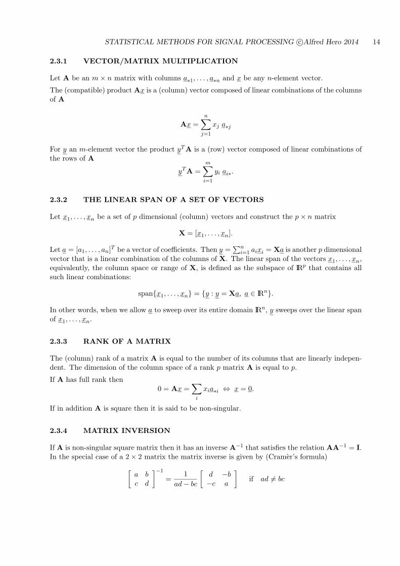
2.3.1 VECTOR/MATRIX MULTIPLICATION
Let A be an m× n matrix with columns a∗1, . . . , a∗n and x be any n-element vector.
The (compatible) product Ax is a (column) vector composed of linear combinations of the columnsof A
Ax =
n∑j=1
xj a∗j
For y an m-element vector the product yTA is a (row) vector composed of linear combinations ofthe rows of A
yTA =
m∑i=1
yi ai∗.
2.3.2 THE LINEAR SPAN OF A SET OF VECTORS
Let x1, . . . , xn be a set of p dimensional (column) vectors and construct the p× n matrix
X = [x1, . . . , xn].
Let a = [a1, . . . , an]T be a vector of coefficients. Then y =
∑ni=1 aixi = Xa is another p dimensional
vector that is a linear combination of the columns of X. The linear span of the vectors x1, . . . , xn,equivalently, the column space or range of X, is defined as the subspace of IRp that contains allsuch linear combinations:
span{x1, . . . , xn} = {y : y = Xa, a ∈ IRn}.
In other words, when we allow a to sweep over its entire domain IRn, y sweeps over the linear spanof x1, . . . , xn.
2.3.3 RANK OF A MATRIX
The (column) rank of a matrix A is equal to the number of its columns that are linearly indepen-dent. The dimension of the column space of a rank p matrix A is equal to p.
If A has full rank then0 = Ax =
∑i
xia∗i ⇔ x = 0.
If in addition A is square then it is said to be non-singular.
2.3.4 MATRIX INVERSION
If A is non-singular square matrix then it has an inverse A−1 that satisfies the relation AA−1 = I.In the special case of a 2× 2 matrix the matrix inverse is given by (Cramer’s formula)[
a bc d
]−1
=1
ad− bc
[d −b−c a
]if ad = bc
STATISTICAL METHODS FOR SIGNAL PROCESSING c⃝Alfred Hero 2014 15
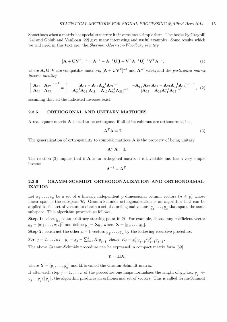
Sometimes when a matrix has special structure its inverse has a simple form. The books by Graybill[24] and Golub and VanLoan [22] give many interesting and useful examples. Some results whichwe will need in this text are: the Sherman-Morrison-Woodbury identity
[A+UVT ]−1 = A−1 −A−1U[I+VTA−1U]−1VTA−1, (1)
where A,U,V are compatible matrices, [A+UVT ]−1 and A−1 exist; and the partitioned matrixinverse identity[
A11 A12
A21 A22
]−1
=
[[A11 −A12A
−122 A21]
−1 −A−111 A12[A22 −A21A
−111 A12]
−1
−A−122 A21[A11 −A12A
−122 A21]
−1 [A22 −A21A−111 A12]
−1
], (2)
assuming that all the indicated inverses exist.
2.3.5 ORTHOGONAL AND UNITARY MATRICES
A real square matrix A is said to be orthogonal if all of its columns are orthonormal, i.e.,
ATA = I. (3)
The generalization of orthogonality to complex matrices A is the property of being unitary,
AHA = I.
The relation (3) implies that if A is an orthogonal matrix it is invertible and has a very simpleinverse
A−1 = AT .
2.3.6 GRAMM-SCHMIDT ORTHOGONALIZATION AND ORTHONORMAL-IZATION
Let x1, . . . , xn be a set of n linearly independent p dimensional column vectors (n ≤ p) whoselinear span is the subspace H. Gramm-Schmidt orthogonalization is an algorithm that can beapplied to this set of vectors to obtain a set of n orthogonal vectors y
1, . . . , y
nthat spans the same
subspace. This algorithm proceeds as follows.
Step 1: select y1as an arbitrary starting point in H. For example, choose any coefficient vector
a1 = [a11, . . . , a1n]T and define y
1= Xa1 where X = [x1, . . . , xn].
Step 2: construct the other n− 1 vectors y2, . . . , y
nby the following recursive procedure:
For j = 2, . . . , n: yj= xj −
∑ji=1Kiyi−1
where Kj = xTj yj−1/yT
j−1yj−1
.
The above Gramm-Schmidt procedure can be expressed in compact matrix form [69]
Y = HX,
where Y = [y1, . . . , y
n] and H is called the Gramm-Schmidt matrix.
If after each step j = 1, . . . , n of the procedure one maps normalizes the length of yj, i.e., y
j←
yj= y
j/∥y
j∥, the algorithm produces an orthonormal set of vectors. This is called Gram-Schmidt
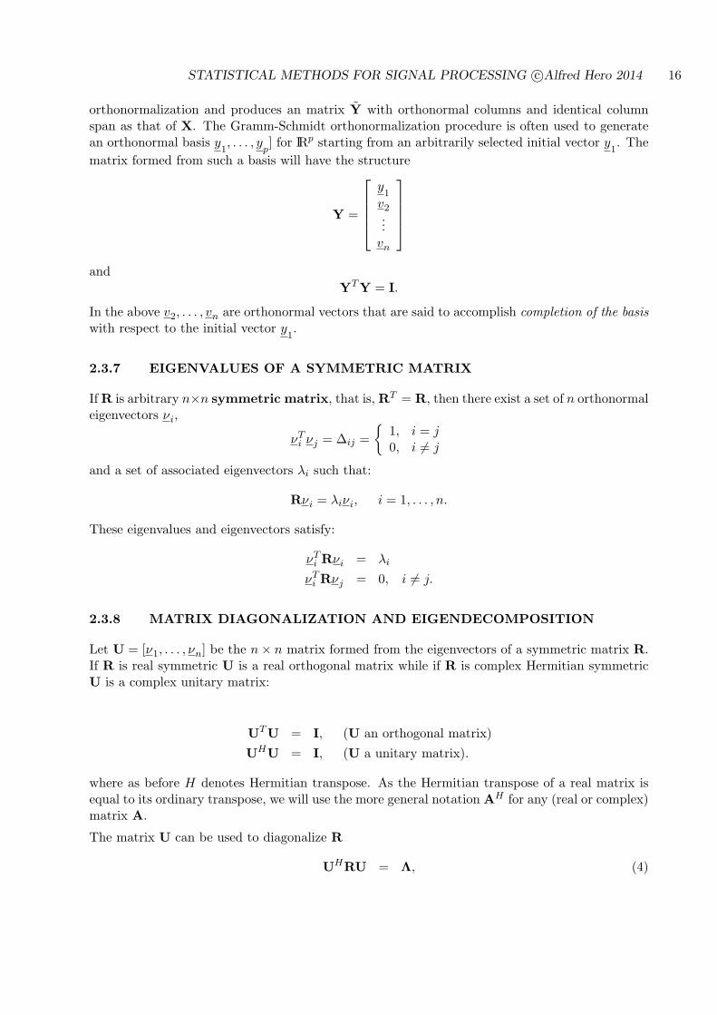
STATISTICAL METHODS FOR SIGNAL PROCESSING c⃝Alfred Hero 2014 16
orthonormalization and produces an matrix Y with orthonormal columns and identical columnspan as that of X. The Gramm-Schmidt orthonormalization procedure is often used to generatean orthonormal basis y
1, . . . , y
p] for IRp starting from an arbitrarily selected initial vector y
1. The
matrix formed from such a basis will have the structure
Y =
y1v2...vn
and
YTY = I.
In the above v2, . . . , vn are orthonormal vectors that are said to accomplish completion of the basiswith respect to the initial vector y
1.
2.3.7 EIGENVALUES OF A SYMMETRIC MATRIX
IfR is arbitrary n×n symmetric matrix, that is, RT = R, then there exist a set of n orthonormaleigenvectors νi,
νTi νj = ∆ij =
{1, i = j0, i = j
and a set of associated eigenvectors λi such that:
Rνi = λiνi, i = 1, . . . , n.
These eigenvalues and eigenvectors satisfy:
νTi Rνi = λi
νTi Rνj = 0, i = j.
2.3.8 MATRIX DIAGONALIZATION AND EIGENDECOMPOSITION
Let U = [ν1, . . . , νn] be the n× n matrix formed from the eigenvectors of a symmetric matrix R.If R is real symmetric U is a real orthogonal matrix while if R is complex Hermitian symmetricU is a complex unitary matrix:
UTU = I, (U an orthogonal matrix)
UHU = I, (U a unitary matrix).
where as before H denotes Hermitian transpose. As the Hermitian transpose of a real matrix isequal to its ordinary transpose, we will use the more general notation AH for any (real or complex)matrix A.
The matrix U can be used to diagonalize R
UHRU = Λ, (4)
STATISTICAL METHODS FOR SIGNAL PROCESSING c⃝Alfred Hero 2014 17
In cases of both real and Hermitian symmetric R the matrix Λ is diagonal and real valued
Λ = diag(λi) =
λ1 . . . 0...
. . ....
0 . . . λn
,where λi’s are the eigenvalues of R.
The expression (4) implies that
R = UΛUH ,
which is called the eigendecomposition of R. As Λ is diagonal, an equivalent summation form forthis eigendecomposition is
R =
n∑i=1
λiνiνHi . (5)
2.3.9 QUADRATIC FORMS AND NON-NEGATIVE DEFINITE MATRICES
For a square symmetric matrix R and a compatible vector x, a quadratic form is the scalar definedby xTRx. The matrix R is non-negative definite (nnd) if for any x
xTRx ≥ 0. (6)
R is positive definite (pd) if it is nnd and ”=” in (6) implies that x = 0, or more explicitly R ispd if
xTRx > 0, x = 0. (7)
Examples of nnd (pd) matrices:
* R = BTB for arbitrary (pd) matrix B
* R symmetric with only non-negative (positive) eigenvalues
Rayleigh Theorem: If A is a nnd n× n matrix with eigenvalues {λi}ni=1 the quadratic form
min(λi) ≤uTAu
uTu≤ max(λi)
where the lower bound is attained when u is the eigenvector of A associated with the minimumeigenvalue of A and the upper bound is attained by the eigenvector associated with the maximumeigenvalue of A.
2.4 POSITIVE DEFINITENESS OF SYMMETRIC PARTITIONED MA-TRICES
If A is a symmetric matrix with partition representation (2) then it is easily shown that
A =
[A11 A12
A21 A22
]=
[I −A12A
−122
O I
]−1 [A11 −A12A
−122 A21 OT
O A22
] [I OT
−A−122 A21 I
]−1
, (8)
as long as A−122 exists. Here O denotes a block of zeros. This implies: if A is positive definite the
matrices A11−A12A−122 A21 and A22 are pd. By using an analogous identity we can conclude that
A22 −A21A−111 A12 and A11 are also pd.
STATISTICAL METHODS FOR SIGNAL PROCESSING c⃝Alfred Hero 2014 18
2.4.1 DETERMINANT OF A MATRIX
If A is any square matrix its determinant is
|A| =∏i
λi
Note: a square matrix is non-singular iff its determinint is non-zero.
If A is partitioned as in (2) and A−111 and A−1
22 exist then
|A| = |A11||A22 −A21A−111 A12| = |A22||A11 −A12A
−122 A21| (9)
This follows from the decomposition (8).
2.4.2 TRACE OF A MATRIX
For any square matrix A = ((aij)) the trace of A is defined as
trace{A} =∑i
aii =∑i
λi
One has an important identity: for compatible matrices A and B
trace{AB} = trace{BA}.
This has the following implication for quadratic forms:
xTRx = trace{xxT R}.
2.4.3 VECTOR DIFFERENTIATION
Differentiation of functions of a vector variable often arise in signal processing and estimationtheory. If h = [h1, . . . , hn]
T is an n × 1 vector and g(h) is a scalar function then the gradient ofg(h), denoted ∇g(h) or ∇hg(h) when necessary for conciseness, is defined as the (column) vectorof partials
∇g =
[∂g
∂h1, . . . ,
∂g
∂hn
]T.
In particular, if c is a constant∇hc = 0,
if x = [x1, . . . , xn]T
∇h(hTx) = ∇h(xTh) = x,
and if B is an n× n matrix
∇h(h− x)TB(h− x) = 2B(h− x).
For a vector valued function g(h) = [g1(h), . . . , gm(h)]T the gradient of g(h) is an m × n matrix.
In particular, for a scalar function g(h), the two applications of the gradient ∇(∇g)T gives then× n Hessian matrix of g, denoted as ∇2g. This yields useful and natural identities such as:
∇2h(h− x)TB(h− x) = 2B.
For a more detailed discussion of vector differentiation the reader is referred to Kay [40].
STATISTICAL METHODS FOR SIGNAL PROCESSING c⃝Alfred Hero 2014 19
2.5 SIGNALS AND SYSTEMS BACKGROUND
Here we review some of the principal results that will be useful for dealing with signals and systemsencountered in this book.
2.5.1 GEOMETRIC SERIES
One of the most useful formulas in discrete time signal and systems engineering is:
n∑i=0
an =1− an+1
1− a, if a = 1;
∞∑i=0
an =1
1− a, if |a| < 1.
2.5.2 LAPLACE AND FOURIER TRANSFORMS OF FUNCTIONS OF A CON-TINUOUS VARIABLE
If h(t), −∞ < t < ∞, a square integrable function of a continuous variable t (usually time) thenits Laplace and Fourier transforms are defined as follows.
The Laplace transform of h is
L{h} = H(s) =
∫ ∞
−∞h(t)e−st dt
where s = σ + jω ∈ Cl is a complex variable.
The Fourier transform of h is
F{h} = H(ω) =
∫ ∞
−∞h(t)e−jωt dt
Note: F{h} = L{h}|s=jω.Example: if h(t) = e−atu(t), for a > 0, then the Laplace transform is
H(s) =
∫ ∞
0e−ate−st dt =
∫ ∞
0e−(a+s)t dt =
−1a+ s
e−(a+st)
∣∣∣∣∞0
=1
a+ s
2.5.3 Z-TRANSFORM AND DISCRETE-TIME FOURIER TRANSFORM (DTFT)
If hk, k = . . . ,−1, 0, 1, . . ., is a square summable function of a discrete variable then its Z-transformand discrete-time Fourier transform (DTFT) are defined as follows.
The Z-transform is
Z{h} = H(z) =
∞∑k=−∞
hkz−k
The DTFT is
F{h} = H(ω) =
∞∑k=−∞
hke−jωk
Note: H(ω) really means H(ejω) and is an abuse of notation
STATISTICAL METHODS FOR SIGNAL PROCESSING c⃝Alfred Hero 2014 20
• F{h} = Z{h}|z=ejω• the DTFT is always periodic in ω with period 2π.
Example: if hk = a|k|, then for |az−1| < 1 and |az| < 1, the Z-transform is
H(z) =∞∑
k=−∞a|k|z−k =
−1∑k=−∞
a−kz−k +∞∑k=0
akz−k
=∞∑k=1
(az)k +∞∑k=0
(az−1)k =az
1− az+
1
1− az−1
Likewise the DTFT is (for |a| < 1):
H(ω) = H(z)|z=ejω =1− a2
1− 2a cosω + a2
2.5.4 CONVOLUTION: CONTINUOUS TIME
If h(t) and x(t) are square integrable functions of a continuous variable t then the convolution ofx and h is defined as
(h ∗ x)(t) =∫ ∞
−∞h(t− τ)x(τ) dτ
Note: The convolution of h and x is a waveform indexed by time t. (h ∗ x)(t) is this waveformevaluated at time t and is frequently denoted h(t) ∗ x(t).Example: h(t) = e−atu(t), for a > 0, (the filter) and x(t) = e−btu(t), for b > 0, (the filter input)then
(h ∗ x)(t) =∫ ∞
−∞e−a(t−τ)e−bτu(t− τ)u(τ) dτ =
(∫ t
0e−a(t−τ)e−bτ dτ
)u(t)
= e−at(∫ t
0e−(b−a)τ dτ
)u(t) = e−at
(−1b− a
e−(b−a)τ∣∣∣∣t0
)u(t) =
e−at − e−bt
b− au(t)
2.5.5 CONVOLUTION: DISCRETE TIME
If hk and xk are square integrable sequences then
hn ∗ xn =
∞∑j=−∞
hjxn−j =
∞∑j=−∞
hn−jxj
hk is a called a “causal” filter if it is zero for negative indices:
hk = 0, k < 0
STATISTICAL METHODS FOR SIGNAL PROCESSING c⃝Alfred Hero 2014 21
2.5.6 CORRELATION: DISCRETE TIME
For time sequences {xk}nk=1 and {yk}nk=1 their temporal correlation is
zn =n∑j=1
xky∗k
2.5.7 RELATION BETWEEN CORRELATION AND CONVOLUTION
The temporal correlation is directly related to the convolution of xk with a filter impulse responsehk where the output of the filter is sampled at time k = n:
zn =n∑j=1
xky∗k =
∞∑j=−∞
xkhn−k = hn ⋆ xn,
where the filter impulse response is equal to the shifted and time reversed signal yk,
hk =
{y∗n−k, k = 1, . . . , n
0, o.w.
The filter hk is called the matched filter and is used for optimal detection of a known signal {yk}in white Gaussian noise.
2.5.8 CONVOLUTION AS A MATRIX OPERATION
Let hk be a causal filter impulse response and let xk be an input starting at time k = 1. Arrangingn outputs zk in a vector z it is easy to see that
z =
zn...z1
=
∑n
j=1 hn−jxj...∑n
j=1 h1−jxj
=
h0 h1 · · · hn−1
0 h0. . . hn−2
.... . . h0 h1
0 · · · 0 h0
xn
...x1
2.6 BACKGROUND REFERENCES
There are many useful textbooks that cover areas of this chapter. I learned elementary linearalgebra from Noble and Daniel [61]. A more advanced book that is focused on computational linearalgebra is Golub and Van Loan [22] which covers many fast and numerically stable algorithmsarising in signal processing. Another nice book on linear algebra with emphasis on statisticalapplications is Graybill [24] that contains lots of useful identities for multivariate Gaussian models.For background on signals and systems Oppenheim and Willsky [62] and Proakis and Manolakis[65] are good elementary textbooks. The encyclopedic book by Moon and Stirling [57] is a goodgeneral resource for mathematical methods in signal processing.
STATISTICAL METHODS FOR SIGNAL PROCESSING c⃝Alfred Hero 2014 22
2.7 EXERCISES
2.1 Let a, b be n × 1 vectors and let C be an invertible n × n matrix. Assuming α is not equalto −1/(aTC−1b) show the following identity
[C+ αabT ]−1 = C−1 −C−1abTC−1α/(1 + αaTC−1b).
2.2 A discrete time LTI filter h(k) is causal when h(k) = 0, k < 0 and anticausal when h(k) =0, k > 0. Show that if |h(k)| < ∞ for all k, the transfer function H(z) =
∑∞k=−∞ h(k)z−k
of a causal LTI has no singularities outside the unit circle, i.e. |H(z)| < ∞, |z| > 1 whilean anticausal LTI has no singularities inside the unit circle, i.e. |H(z)| <∞, |z| < 1. (Hint:generalized triangle inequality |
∑i ai| ≤
∑|ai|)
2.3 A discrete time LTI filter h(k) is said to be BIBO stable when∑∞
k=−∞ |h(k)| < ∞. Define
the transfer function (Z-transform) H(z) =∑∞
k=−∞ h(k)z−k, for z a complex variable.
(a) Show that H(z) has no singularities on the unit circle, i.e |H(z)| <∞, |z| = 1.
(b) Show that if a BIBO stable h(k) is causal then H(z) has all its singularities (poles)strictly inside the unit circle, i.e |H(z)| <∞, |z| ≥ 1.
(c) Show that if a BIBO stable h(k) is anticausal, i.e. h(k) = 0, k > 0, then H(z) has all itssingularities (poles) strictly outside the unit circle, i.e |H(z)| <∞, |z| ≤ 1.
2.4 If you are only given the mathematical form of the transfer function H(z) of an LTI, and nottold whether it corresponds to an LTI which is causal, anticausal, or stable, then it is notpossible to uniquely specify the impulse response {hk}k. This simple example illustration thisfact. The regions {z : |z| > a} and {z : |z| ≤ a}, specified in (a) and (b) are called the regionsof convergence of the filter and specify whether the filter is stable, causal or anticausal.
Let H(z) be
H(z) =1
1− az−1
(a) Show that if the LTI is causal, then for |z| > |a| you can write H(z) as the convergentseries
H(z) =∞∑k=0
akz−k, |z| > |a|
which corresponds to hk = ak, k = 0, 1, . . . and hk = 0, k < 0.
(b) Show that if the LTI is anticausal, then for |z| < |a| you can write H(z) as the convergentseries
H(z) = −∞∑k=0
a−kzk+1, |z| < |a|
which corresponds to hk = −a−k, k = 1, 2 . . . and hk = 0, k ≥ 0.
(c) Show that if |a| < 1 then the causal LTI is BIBO stable while the anti-causal LTI isBIBO unstable while if |a| > 1 then the reverse is true. What happens to stability when|a| = 1?
2.5 An LTI has transfer function
H(z) =3− 4z−1
1− 3.5z−1 + 1.5z−2
STATISTICAL METHODS FOR SIGNAL PROCESSING c⃝Alfred Hero 2014 23
(a) If you are told that the LTI is stable specify the region of convergence (ROC) in thez-plane, i.e. specify the range of values of |z| for which |H(z)| < ∞, and specify theimpulse response.
(b) If you are told that the LTI is causal specify the region of convergence (ROC) in thez-plane, and specify the impulse response.
(c) If you are told that the LTI is anticausal specify the region of convergence (ROC) in thez-plane, and specify the impulse response.
End of chapter
STATISTICAL METHODS FOR SIGNAL PROCESSING c⃝Alfred Hero 2014 24
Estimation, detection and classification can be grouped under the broad heading of statisticalinference which is the process of inferring properties about the distribution of a random variableX given a realization x, which is also called a data sample, a measurement, or an observation. Akey concept is that of the statistical model which is simply a hypothesized probability distributionor density function f(x) for X. Broadly stated statistical inference explores the possibility offitting a given model to the data x. To simplify this task it is common to restrict f(x) to a class ofparameteric models {f(x; θ)}θ∈Θ, where f(x; •) is a known function and θ is a vector of unknownparameters taking values in a parameter space Θ. In this special case statistical inference boilsdown to inferring properties of the true value of θ parameterizing f(x; θ) that generated the datasample x.
In this chapter we discuss several models that are related to the ubiquitous Gaussian distribution,the more general class of exponential families of distributions, and the important concept of asufficient statistic for infering properties about θ.
3.1 THE GAUSSIAN DISTRIBUTION AND ITS RELATIVES
The Gaussian distribution and its close relatives play a major role in parameteric statistical in-ference due to the relative simplicity of the Gaussian model and its broad applicability (recall theCentral Limit Theorem!). Indeed, in engineering and science the Gaussian distribution is probablythe most commonly invoked distribution for random measurements. The Gaussian distribution isalso called the Normal distribution. The probability density function (pdf) of a Gaussian randomvariable (rv) X is parameterized by two parameters, θ1 and θ2, which are the location parameter,denoted µ (µ ∈ IR), and the (squared) scale parameter, denoted σ2 (σ2 > 0). The pdf of thisGaussian rv has the form
f(x;µ, σ2) =1√2πσ
e−(x−µ)2
2σ2 , −∞ < x <∞
When µ = 0 and σ2 = 1, X is said to be a standard Gaussian (Normal) rv. A Gaussian randomvariable with location parameter µ and scale parameter σ > 0 can be represented by
X = σZ + µ, (10)
where Z is a standard Gaussian rv.
The cumulative density function (cdf) of a standard Gaussian random variable Z is denoted N (z)and is defined in the conventional manner
N (z) = P (Z ≤ z).
Equivalently,
N (z) =
∫ z
−∞
1√2πe−
v2
2 dv.
Using (10) the cdf of a non-standard Gaussian rv X with parameters µ and σ2 can be expressedin terms of the cdf N (z) of a standard Gaussian rv Z:
P (X ≤ x) = P ((X − µ)/σ︸ ︷︷ ︸Z
≤ (x− µ)/σ) = N(x− µσ
)
STATISTICAL METHODS FOR SIGNAL PROCESSING c⃝Alfred Hero 2014 25
The standard Normal cdf N (x) can be related to the error function or error integral [1]: erf(u) =2√π
∫ u0 e
−t2dt, x ≥ 0, through the relation
N (x) =
{12[1 + erf(|x|/
√2)] x ≥ 0
12[1− erf(|x|/
√2)], x < 0
.
For positive integer order ν, the moments of a standard Gaussian random variable Z are [34, 13.3]
E[Zν ] =
{(ν − 1)(ν − 3) · · · 3 · 1, ν even
0, ν odd
where E[g(Z)] =∫∞−∞ g(z)f(z)dz denotes statistical expectation of the rv g(Z) under the pdf
f(z) for rv Z. These moment relations can easily be derived by looking at the coefficients of(ju)k/k!, k = 1, 2, . . . in the power series expansion about ju = 0 of the characteristic functionΦZ(u) = E[ejuZ ] = e−u
2/2.
In particular, using (10), this implies that the first and second moments of a non-standard Gaussianrv X are E[X] = µ and E[X2] = µ2 + σ2, respectively. Thus for a Gaussian rv X we can identifythe (ensemble) mean E[X] = µ and variance var(X) = E[(X − E[X])2] = E[X2] − E2[X] = σ2
as the location and (squared) scale parameters, respectively, of the pdf f(x;µ, σ2) of X. In thesequel we will need the following expression for the (non-central) mean deviation E[|X + a|] forGaussian X [35, 29.6]:
E[|X + a|] =√
2
πe−a
2/2 + a(1− 2N (−a)). (11)
In referring to rv’s and operations on rv’s in this book the following compact notations are some-times used:
* “X is distributed as a Gaussian random variable with mean µ and variance σ2”
X ∼ N (µ, σ2) (12)
* “X is equal to a scaled and shifted standard Gaussian random variable”
X = a Z︸︷︷︸N (0,1)
+b ⇔ X ∼ N (b, a2)
or, in shorthand notation,
X = a N (0, 1) + b ⇔ X ∼ N (b, a2). (13)
For example, in the following shorthand notation X1, . . . , Xn are independent identically dis-tributed (iid) N (0, 1) rv’s
n∑i=1
N (0, 1) =n∑i=1
Xi.
Note that the above is an abuse of notation since N (0, 1) is being used to denote both a Gaussianprobability distribution in (12) and a Gaussian random variable in (13). As in all abuses of this
STATISTICAL METHODS FOR SIGNAL PROCESSING c⃝Alfred Hero 2014 26
type the ambiguity is resolved from the context: we will never write N (0, 1) into an algebraic orother type of equation like the one in (13) when N (0, 1) is meant to denote a Gaussian distributionfunction as opposed to a Gaussian random variable.
Other notational shortcuts are the following. When we write
N (v) = α
we mean that “the cdf of a N (0, 1) rv equals α when evaluated at a point v ∈ IR.” Likewise
N−1(α) = v
is to be read as “the inverse cdf of a N (0, 1) rv equals v when evaluated at a point α ∈ [0, 1].”Finally, by
X ∼ Nn(µ, R)
we mean “X is distributed as an n-dimensional Gaussian random vector with mean µ and covari-ance matrix R”
3.1.1 MULTIVARIATE GAUSSIAN DISTRIBUTION
When one passes an i.i.d. Gaussian random sequence through a linear filter the output remainsGaussian but is no longer i.i.d; the filter smooths the input and introduces correlation. Remarkably,if the input to the filter is Gaussian then the output is also Gaussian, i.e., the joint distributionof any p samples of the output is multivariate Gaussian. To be specific, a random vector X =[X1, . . . , Xp]
T is multivariate Gaussian with mean parameter µ and covariance matrix parameterΛ if it has a joint density of the form
f(x) =1
(2π)p/2|Λ|1/2exp
(−1
2(x− µ)Λ−1(x− µ)
)x ∈ IRp. (14)
where |Λ| denotes the the determinant of Λ. The p-variate Gaussian distribution depends onp(p + 3)/2 parameters, which we can concatenate into a parameter vector θ consisting of the pelements of the mean vector
µ = [µ1, . . . , µp]T = E[X],
and the p(p+ 1)/2 distinct parameters of the symmetric positive definite p× p covariance matrix
Λ = cov(Z) = E[(Z − µ)(Z − µ)T
].
Some useful facts about the multivariate Gaussian random variables are (for derivations of theseproperties see Morrison [58]):
• Unimodality and symmetry of the Gaussian density: The multivariate Gaussian density(14) is unimodal (has a unique maximum) and is symmetric about its mean parameter.
• Uncorrelated Gaussians are independent: When the covariance matrix Λ is diagonal, i.e.,cov(Xi, Xj) = 0, i = j, then the multivariate Gaussian density reduces to a product of univariatedensities
f(X) =n∏i=1
f(Xi)
STATISTICAL METHODS FOR SIGNAL PROCESSING c⃝Alfred Hero 2014 27
where
f(Xi) =1√2πσi
e− 1
2σ2i
(Xi−µi)2
is the univariate Gaussian density with σ2i = var(Xi). Thus uncorrelated Gaussian random vari-ables are in fact independent random variables.
• Marginals of a Gaussian density are Gaussian: If X = [X1, . . . , Xm]T is multivariate
Gaussian then any subset of the elements of X is also Gaussian. In particular X1 is univariateGaussian and [X1, X2] is bivariate Gaussian.
• Linear combination of Gaussian random variables are Gaussian: LetX = [X1, . . . , Xm]T
be a multivariate Gaussian random vector and letH be a p×m non-random matrix. Then Y = HXis a vector of linear combinations of the Xi’s. The distribution of Y is multivariate (p-variate)Gaussian with mean µ
Y= E[Y ] = Hµ and p× p covariance matrix ΛY = cov(Y ) = Hcov(X)HT .
• A vector of i.i.d. zero mean Gaussian random variables is invariant to rotation: LetX = [X1, . . . , Xm]
T be vector of zero mean Gaussian random variables with covariance cov(X) =σ2I. If U is an orthogonal m×m matrix, i.e., UTU = I, then Y = UTX has the same distributionas X.
• The conditional distribution of a Gaussian given another Gaussian is Gaussian: Letthe vector ZT = [XT , Y T ] = [X1, . . . , Xp, Y1, . . . , Yq]
T be multivariate ((p + q)-variate) Gaussianwith mean parameters µT
Z= [µT
X, µT
Y] and covariance parameters ΛZ . Then the conditional density
fY |X(y|x) of Y given X = x is multivariate (q-variate) Gaussian of the form (14) with mean andcovariance parameters µ and Λ respectively given by (15) and (16) below.
• Conditional mean of a Gaussian given another Gaussian is linear and conditionalcovariance is constant: For the aforementioned multivariate Gaussian vector ZT = [XT , Y ]T
partition its covariance matrix as follows
ΛZ =
[ΛX ΛX,Y
ΛTX,Y ΛY
],
where ΛX = cov(X) = E[(X − µX)(X − µ
X)T ] is p × p, ΛY = cov(Y ) = E[(Y µ
Y)(Y − µ
Y)T ] is
q × q, and ΛX,Y = covθ(X,Y ) = E[(X − µX)(Y − µ
Y)T ] is p × q. The mean of the multivariate
Gaussian conditional density f(y|x), the conditional mean, is linear in x
µY |X(x) = E[Y |X = x] = µ
Y+ΛT
X,YΛ−1X (x− µ
X) (15)
and the conditional covariance does not depend on x
ΛY |X = cov(Y |X = x) = ΛY −ΛTX,YΛ
−1X ΛX,Y . (16)
3.1.2 CENTRAL LIMIT THEOREM
One of the most useful results in statistics is the central limit theorem, abbreviated to CLT.This theorem allows one to approximate the distribution of sums of i.i.d. finite variance randomvariables by a Gaussian distribution. Below we give a general version of the CLT that applies tovector valued r.v.s. For a simple proof of the scalar case see Mood, Graybill and Boes [56]. Forproof in the multivariate case see Serfling [Ch. 1][72], which also covers the CLT for the non i.i.d.case.
STATISTICAL METHODS FOR SIGNAL PROCESSING c⃝Alfred Hero 2014 28
(Lindeberg-Levy) Central Limit Theorem: Let {Xi}ni=1 be i.i.d. random vectors in IRp withcommon mean E[Xi] = µ and finite positive definite covariance matrix cov(Xi) = Λ. Then as n
goes to infinity the distribution of the random vector Zn = n−1/2∑n
i=1(Xi − µ) converges to ap-variate Gaussian distribution with zero mean and covariance Λ.
The CLT can also be expressed in terms of the sample mean X = X(n) = n−1∑n
i=1Xi: as n→∞√n(X(n)− µ) −→ Z
where Z is a zero mean Gaussian random vector with covariance matrix Λ. Thus, for large butfinite n, X is approximately Gaussian
X ≈ (Z/√n+ µ),
with mean µ and covariance Λ/n. For example, in the case of a scalar Xi, the CLT gives theuseful large n approximation
P (n−1n∑i=1
Xi ≤ y) ≈∫ y
−∞
1√2πσ2/n
exp
(−(y − µ)2
2σ2/n
)dy.
The approximation error can be bounded by using the Berry-Esseen Theorems. See Serfling [72]for details.
3.1.3 CHI-SQUARE
The (central) Chi-square density with k degrees of freedom (df) is of the form:
fθ(x) =1
2k/2Γ(k/2)xk/2−1e−x/2, x > 0, (17)
where θ = k, a positive integer. Here Γ(u) denotes the Gamma function,
Γ(u) =
∫ ∞
0xu−1e−xdx,
For n integer valued Γ(n+ 1) = n! = n(n− 1) . . . 1 and Γ(n+ 1/2) = (2n−1)(2n−3)...5·3·12n
√π.
If Zi ∼ N (0, 1) are i.i.d., i = 1, . . . , n, then X =∑n
i=1 Z2i is distributed as Chi-square with n
degrees of freedom (df). Our shorthand notation for this is
n∑i=1
[N (0, 1)]2 = χn. (18)
This characterization of a Chi square r.v. is sometimes called a stochastic representation since itis defined via operations on other r.v.s. The fact that (17) is the density of a sum of squares ofindependent N (0, 1)’s is easily derived. Start with the density function f(z) = e−z
2/2/√2π of a
standard Gaussian random variable Z. Using the relation (√2πσ)−1
∫∞−∞ e−u
2/(2σ2)du = 1, the
characteristic function of Z2 is simply found as ΦZ2(u) = E[ejuZ2] = (1 + j2u)−1/2. Applying
the summation-convolution theorem for independent r.v.s Yi, Φ∑Yi(u) =
∏ΦYi(u), we obtain
Φ∑ni=1 Z
2i(u) = (1+ j2u)−n/2. Finally, using a table of Fourier transform relations, identify (17) as
the inverse fourier transform of Φ∑ni=1 Z
2i(u).
STATISTICAL METHODS FOR SIGNAL PROCESSING c⃝Alfred Hero 2014 29
Some useful properties of the Chi-square random variable are as follows:
* E[χn] = n, var(χn) = 2n
* Asymptotic relation for large n:
χn =√2nN (0, 1) + n
* χ2 an exponential r.v. with mean 2, i.e. X = χ2 is a non-negative r.v. with probability densityf(x) = 1
2e−x/2.
*√χ2 is a Rayleigh distributed random variable.
3.1.4 GAMMA
The Gamma density function is
fθ(x) =λr
Γ(r)xr−1e−λx, x > 0,
where θ denotes the pair of parameters (λ, r), λ, r > 0. Let {Yi}ni=1 be i.i.d. exponentiallydistributed random variables with mean 1/λ, specifically Yi has density
fλ(y) = λe−λy, y > 0.
Then the sum X =∑n
i=1 Yi has a Gamma density f(λ,n). Other useful properties of a Gammadistributed random variable X with parameters θ = (λ, r) include:
* Eθ[X] = r/λ
* varθ(X) = r/λ2
* The Chi-square distribution with k df is a special case of the Gamma distribution obtained bysetting Gamma parameters as follows: λ = 1/2 and r = k/2.
3.1.5 NON-CENTRAL CHI SQUARE
The sum of squares of independent Gaussian r.v.s with unit variances but non-zero means is calleda non-central Chi-square r.v. Specifically, if Zi ∼ N (µi, 1) are independent, i = 1, . . . , n, thenX =
∑ni=1 Z
2i is distributed as non-central Chi-square with n df and non-centrality parameter
δ =∑n
i=1 µ2i . In our shorthand we write
n∑i=1
[N (0, 1) + µi]2 =
n∑i=1
[N (µi, 1)]2 = χn,δ. (19)
The non-central Chi-square density has no simple expression of closed form. There are some usefulasymptotic relations, however:
* E[χn,δ] = n+ δ, var(χn,δ) = 2(n+ 2δ)
*√χ2,µ21+µ
22is a Rician r.v.
STATISTICAL METHODS FOR SIGNAL PROCESSING c⃝Alfred Hero 2014 30
3.1.6 CHI-SQUARE MIXTURE
The distribution of the sum of squares of independent Gaussian r.v.s with zero mean but differentvariances is not closed form either. However, many statisticians have studied and tabulated thedistribution of a weighted sum of squares of i.i.d. standard Gaussian r.v.s Z1, . . . , Zn, Zi ∼ N (0, 1).Specifically, the following has a (central) Chi-square mixture (also known as the Chi-bar square[34]) with n degrees of freedom and mixture parameter c = [c1, . . . , cn]
T , ci ≥ 0:
n∑i=1
ci∑j cj
Z2i = χn,c
An asymptotic relation of interest to us will be:
* E[χn,c] = 1, , var(χn,c) = 2∑N
i=1
(ci∑j ci
)2Furthermore, there is an obvious a special case where the Chi square mixture reduces to a scaled(central) Chi square: χn,c1 =
1n χn for any c = 0.
3.1.7 STUDENT-T
For Z ∼ N (0, 1) and Y ∼ χn independent r.v.s the ratio X = Z/√Y/n is called a Student-t r.v.
with n degrees of freedom, denoted Tn. Or in our shorthand notation:
N (0, 1)√χn/n
= Tn.
The density of Tn is the Student-t density with n df and has the form
fθ(x) =Γ([n+ 1]/2)
Γ(n/2)
1√nπ
1
(1 + x2/n)(n+1)/2, x ∈ IR,
where θ = n is a positive integer. Properties of interest to us are:
* E[Tn] = 0 (n > 1), var(Tn) = nn−2 (n > 2)
* Asymptotic relation for large n:
Tn ≈ N (0, 1).
For n = 1 the mean of Tn does not exist and for n ≤ 2 its variance is infinite.
3.1.8 FISHER-F
For U ∼ χm and V ∼ χn independent r.v.s the ratio X = (U/m)/(V/n) is called a Fisher-F r.v.with m,n degrees of freedom, or in shorthand:
χm/m
χn/n= Fm,n.
The Fisher-F density with m and n df is defined as
fθ(x) =Γ([m+ n]/2)
Γ(m/2)Γ(n/2)
(mn
)m/2 x(m−2)/2
(1 + mn x)
(m+n)/2, x > 0
STATISTICAL METHODS FOR SIGNAL PROCESSING c⃝Alfred Hero 2014 31
where θ = [m,n] is a pair of positive integers. It should be noted that moments E[Xk] of ordergreater than k = n/2 do not exist. A useful asymptotic relation for n large and n≫ m is
Fm,n ≈ χm.
3.1.9 CAUCHY
The ratio of independent N (0, 1) r.v.’s U and V is called a standard Cauchy r.v.
X = U/V ∼ C(0, 1).
It’s density has the form
f(x) =1
π
1
1 + x2x ∈ IR
. If θ = [µ, σ] are location and scale parameters (σ > 0) fθ(x) = f((x − µ)/σ) is a translatedand scaled version of the standard Cauchy density denoted C(µ, σ2). Some properties of note:(1) the Cauchy distribution has no moments of any (positive) integer order; and (2) the Cauchydistribution is the same as a Student-t distribution with 1 d.f.
3.1.10 BETA
For U ∼ χm and V ∼ χn independent Chi-square r.v.s with m and n df, respectively, the ratioX = U/(U + V ) has a Beta distribution, or in shorthand
χmχm + χn
= B(m/2, n/2)
where B(p, q) is a r.v. with Beta density having paramaters θ = [p, q]. The Beta density has theform
fθ(x) =1
βr,txr−1(1− x)t−1, x ∈ [0, 1]
where θ = [r, t] and r, t > 0. Here βr,t is the Beta function:
βr,t =
∫ 1
0xr−1(1− x)t−1dx =
Γ(r)Γ(t)
Γ(r + t).
Some useful properties:
* The special case of m = n = 1 gives rise to X an arcsin distributed r.v.
* Eθ[B(p, q)] = p/(p+ q)
* varθ(B(p, q)) = pq/((p+ q + 1)(p+ q)2)
3.2 REPRODUCING DISTRIBUTIONS
A random variable X is said to have a reproducing distribution if the sum of two independentrealizations, say X1 and X2, of X have the same distribution, possibly with different parametervalues, as X. A Gaussian r.v. has a reproducing distribution:
N (µ1, σ21) +N (µ2, σ
22) = N (µ1 + µ2, σ
21 + σ22),
STATISTICAL METHODS FOR SIGNAL PROCESSING c⃝Alfred Hero 2014 32
which follows from the fact that the convolution of two Gaussian density functions is a Gaus-sian density function [56]. Noting the stochastic representations (18) and (19) of the Chi squareand non-central Chi square distributions, respectively, it is obvious that they are reproducingdistributions:
*χn + χm = χm+n, if χm, χn are independent.
*χm,δ1 + χn,δ2 = χm+n,δ1+δ2 , if χm,δ1 , χn,δ2 are independent.
The Chi square mixture, Fisher-F, and Student-t are not reproducing densities.
3.3 FISHER-COCHRAN THEOREM
This result gives a very useful tool for finding the distribution of quadratic forms of Gaussianrandom variables. A more general result that covers the joint distribution of quadratic forms isgiven in [66].
Theorem 1 Let X = [X1, . . . , Xn]T be a vector of iid. N (0, 1) rv’s and let A be a symmetric
idempotent matrix (AA = A) of rank p. Then
XTAX = χp
A simple proof is given below.
Proof: Let A = UΛUT be the eigendecomposition of A. Then
* All eigenvalues λi of A are either 0 or 1
AA = UΛUTU︸ ︷︷ ︸=I
ΛUT
= UΛ2UT = UΛUT
and therefore
XTAX = XTUΛ UTX︸ ︷︷ ︸Z=Nn(0,I)
=
n∑i=1
λiZ2i =
p∑i=1
[N (0, 1)]2
⋄
3.4 SAMPLE MEAN AND SAMPLE VARIANCE
Let Xi’s be i.i.d. N (µ, σ2) r.v.’s. The sample mean and sample variance respectively approximatethe location µ and spread σ of the population.
* Sample mean: X = n−1∑n
i=1Xi
* Sample variance: s2 = 1n−1
∑ni=1(Xi −X)2
STATISTICAL METHODS FOR SIGNAL PROCESSING c⃝Alfred Hero 2014 33
In the Gaussian case the joint distribution of the sample mean and variance can be specified.
(1). X = N (µ, σ2/n)
(2). s2 = σ2
n−1 χn−1
(3). X and s2 are independent rv’s.
These results imply that a weighted ratio of sample mean and sample variance is distributed asStudent t.
X − µs/√n
= Tn−1.
Proof of assertions (2) and (3): In view of the representation (13), it suffices consider the the caseof a standard Gaussian sample: µ = 0 and σ = 1.
First we show that the sample mean and the sample variance are independent random variables.Define the vector of random variables Y = [Y1, . . . , Yn]
T as follows. First define
Y1 =√nX = hT1X,
whereh1 = [1/
√n, . . . , 1/
√n]T .
Note that h1 has unit norm. Next apply the Gramm-Schmidt orthonormalization procedure ofSec. 2.3.6 to complete the basis with respect to h1. This generates n − 1 vectors h2, . . . , hn thatare orthonormal, mutually orthogonal, and orthogonal to h1. The random vector Y is now definedas
Y = HTX
where H = [h1, . . . , hn] is an n× n orthogonal matrix.
Since, X = HY, the orthogonality of H implies the following properties
1. The Yi’s are zero mean unit variance independent Gaussian random variables: Y ∼ Nn(0, I)2. Y TY = XTX
As Y 1 =√nX Property 1 implies that X is independent of Y2, . . . , Yn. Furthermore, using the
equivalence:n∑i=1
(Xi −X)2 =
n∑i=1
X2i − n(X)2,
Property 2 and the definition of Y1 imply that
n∑i=1
(Xi −X)2 =
n∑i=1
Y 2i − Y 2
1 = Y 22 + · · ·+ Y 2
n , (20)
that is, the sample variance is only a function of Y2, . . . , Yn and is therefore independent of Y1 =the sample mean.
Furthermore, as Y2, . . . , Yn are independent N (0, 1) random variables, the representation (20)implies that the (normalized) sample variance has a Chi-square distribution with n− 1 degrees offreedom.
This completes the proof of assertions (2) and (3). ⋄
STATISTICAL METHODS FOR SIGNAL PROCESSING c⃝Alfred Hero 2014 34
The Chi-square property in assertion (3) can also be shown directly using the Fisher-Cochrantheorem (Thm. 1). Note that the normalized sample variance on the extreme left of the equalities(20) can be expressed as a quadratic form
[X − 1X]T [X − 1X] = XT [I− 11T1
n]︸ ︷︷ ︸
idempotent
[I− 11T1
n]XT
= XT [I− 11T1
n]︸ ︷︷ ︸
orth. proj.
X
where 1 = [1, . . . , 1]T . Observe: since rank[I− 11T 1n ] = n− 1, we have that [X − 1X]T [X − 1X] =
(n− 1) s2 is χn−1.
3.5 SUFFICIENT STATISTICS
Many detection/estimation/classification problems have the following common structure. A con-tinuous time waveform {x(t) : t ∈ IR} is measured at n time instants t1, . . . , tn producing thevector
x = [x1, . . . , xn]T ,
where xi = x(ti). The vector x is modelled as a realization of a random vector X with a jointdistribution which is of known form but depends on a handful (p) of unknown parameters θ =[θ1, . . . , θp]
T .
More concisely:
* X = [X1, . . . , Xn]T , Xi = X(ti), is a vector of random measurements or observations taken over
the course of the experiment
* X is sample or measurement space of realizations x of X
* B is the event space induced by X, e.g., the Borel subsets of IRn
* θ ∈ Θ is an unknown parameter vector of interest
* Θ is parameter space for the experiment
* Pθ is a probability measure on B for given θ. {Pθ}θ∈Θ is called the statistical model for theexperiment.
The probability model induces the joint cumulative distribution function (j.c.d.f.) associated withX
FX(x; θ) = Pθ(X1 ≤ x1, . . . , Xn ≤ xn),
which is assumed to be known for any θ ∈ Θ. When X is a continuous random variable the j.c.d.f.is specified by the joint probability density function (j.p.d.f.) that we will write in several differentways, depending on the context: fθ(x) or f(x; θ), or, when we need to explicitly call out the r.v.X, fX(x; θ). We will denote by Eθ[Z] the statistical expectation of a random variable Z withrespect to the j.p.d.f. fZ(z; θ)
Eθ[Z] =
∫zfZ(z; θ)dz.
The family of functions {f(x; θ)}x∈X ,θ∈Θ then defines the statistical model for the experiment.
STATISTICAL METHODS FOR SIGNAL PROCESSING c⃝Alfred Hero 2014 35
The general objective of statistical inference can now be stated. Given a realization x of X inferproperties of θ knowing only the parametric form of the statistical model. Thus we will want tocome up with a function, called an inference function, which maps X to subsets of the parameterspace, e.g., an estimator, classifier, or detector for θ. As we will see later there are many ways todesign inference functions but a more fundamental question is: are there any general propertiesthat good inference functions should have? One such property is that the inference function onlyneed depend on the n-dimensional data vector X through a lower dimensional version of the datacalled a sufficient statistic.
3.5.1 SUFFICIENT STATISTICS AND THE REDUCTION RATIO
First we define a statistic as any function T = T (X) of the data (actually, for T to be a validrandom variable derived from X it must be a measurable function, but this theoretical technicalityis beyond our scope here).
There is a nice interpretation of a statistic in terms of its memory storage requirements. Assumethat you have a special computer that can store any one of the time samples in X = [X1, . . . , Xn],Xk = X(tk) say, in a ”byte” of storage space and the time stamp tk in another ”byte” of storagespace. Any non-invertible function T , e.g., which maps IRn to a lower dimensional space IRm,can be viewed as a dimensionality reduction on the data sample. We can quantify the amount ofreduction achieved by T by defining the reduction ratio (RR):
RR =# bytes of storage required for T (X)
# bytes of storage required for X
This ratio is a measure of the amount of data compression induced by a specific transformationT . The number of bytes required to store X with its time stamps is:
Define X(i) = as the i-th largest element of X. The X(i)’s satisfy: X(1) ≥ X(2) ≥ . . . ≥ X(n)
and are nothing more than a convenient reordering of the data sample X1, . . . , Xn. The X(i)’s arecalled the rank ordered statistics and do not carry time stamp information. The following tableillustrates the reduction ratio for some interesting cases
Statistic used Meaning in plain english Reduction ratioT (X) = [X1, . . . , Xn]
T , entire data sample RR = 1T (X) = [X(1), . . . , X(n)]
T , rank ordered sample RR = 1/2
T (X) = X, sample mean RR = 1/(2n)
T (X) = [X, s2]T , sample mean and variance RR = 1/n
A natural question is: what is the maximal reduction ratio one can get away with without lossof information about θ? The answer is: the ratio obtained by compression to a quantity called aminimal sufficient statistic. But we are getting ahead of ourselves. We first need to define a plainold sufficient statistic.
STATISTICAL METHODS FOR SIGNAL PROCESSING c⃝Alfred Hero 2014 36
3.5.2 DEFINITION OF SUFFICIENCY
Here is a warm up before making a precise definition of sufficiency. T = T (X) is a sufficientstatistic (SS) for a parameter θ if it captures all the information in the data sample useful forinferring the value of θ. To put it another way: once you have computed a sufficient statistic youcan store it and throw away the original sample since keeping it around would not add any usefulinformation.
More concretely, let X have a cumulative distribution function (CDF) FX(x; θ) depending on θ.A statistic T = T (X) is said to be sufficient for θ if the conditional CDF of X given T = t is nota function of θ, i.e.,
FX|T (x|T = t; θ) = G(x, t), (21)
where G is a function that does not depend on θ.
Specializing to a discrete valued X with probability mass function pθ(x) = Pθ(X = x), a statisticT = T (X) is sufficient for θ if
Pθ(X = x|T = t) = G(x, t). (22)
For a continuous r.v. X with pdf f(x; θ), the condition (21) for T to be a sufficient statistic (SS)becomes:
fX|T (x|t; θ) = G(x, t). (23)
Sometimes the only sufficient statistics are vector statistics, e.g. T (X) = T (X) = [T1(X), . . . , TK(X)]T .In this case we say that the Tk’s are jointly sufficient for θ
The definition (21) is often difficult to use since it involves derivation of the conditional distributionof X given T . When the random variable X is discrete or continuous a simpler way to verifysufficiency is through the Fisher factorization (FF) property [66]
Fisher factorization (FF): T = T (X) is a sufficient statistic for θ if the probability densityfX(x; θ) of X has the representation
fX(x; θ) = g(T, θ) h(x), (24)
for some non-negative functions g and h. The FF can be taken as the operational definition ofa sufficient statistic T . An important implication of the Fisher Factorization is that when thedensity function of a sample X satisfies (24) then the density fT (t; θ) of the sufficient statistic Tis equal to g(t, θ) up to a θ-independent constant q(t) (see exercises at end of this chapter):
fT (t; θ) = g(t, θ)q(t).
Examples of sufficient statistics:
Example 1 Entire sample
X = [X1, . . . , Xn]T is sufficient but not very interesting
Example 2 Rank ordered sample
STATISTICAL METHODS FOR SIGNAL PROCESSING c⃝Alfred Hero 2014 37
X(1), . . . , X(n) is sufficient when Xi’s i.i.d.
Proof: Since Xi’s are i.i.d., the joint pdf is
fθ(x1, . . . , xn) =
n∏i=1
fθ(xi) =
n∏i=1
fθ(x(i)).
Hence sufficiency of the rank ordered sample X(1), . . . , X(n) follows from Fisher factorization.
Example 3 Binary likelihood ratios
Let θ take on only two possible values θ0 and θ1, e.g., a bit taking on the values “0” or “1” in acommunication link. Then, as f(x; θ) can only be f(x; θ0) or f(x; θ1), we can reindex the pdf asf(x; θ) with the scalar parameter θ ∈ Θ = {0, 1}. This gives the binary decision problem: “decidebetween θ = 0 versus θ = 1.” If it exists, i.e. it is finite for all values of X, the “likelihood ratio”
Λ(X) = f1(X)/f0(X) is sufficient for θ, where f1(x)def= f(x; 1) and f0(x)
def= f(x; 0).
Proof: Express fθ(X) as function of θ, f0, f1, factor out f0, identify Λ, and invoke FF
fθ(X) = θf1(X) + (1− θ)f0(X)
=
θΛ(X) + (1− θ)︸ ︷︷ ︸g(T,θ)
f0(X)︸ ︷︷ ︸h(X)
.
⋄Therefore to discriminate between two values θ1 and θ2 of a parameter vector θ we can throw awayall data except for the scalar sufficient statistic T = Λ(X)
Example 4 Discrete likelihood ratios
Let Θ = {θ1, . . . , θp} and assume that the vector of p− 1 likelihood ratios
T (X) =
[fθ1(X)
fθp(X), . . . ,
fθp−1(X)
fθp(X)
]T= [Λ1(X), . . . ,Λp−1(X)]T
is finite for all X. Then this vector is sufficient for θ. An equivalent way to express this vectoris as the sequence {Λθ(X)}θ∈Θ = Λ1(X), . . . ,Λp−1(X), and this is called the likelihood trajectoryover θ.
Proof
Define the p − 1 element selector vector uθ = ek when θ = θk, k = 1, . . . , p − 1 (recall thatek = [0, . . . , 0, 1, 0, . . . 0]T is the k-th column of the (p− 1)× (p− 1) identity matrix). Now for anyθ ∈ Θ we can represent the j.p.d.f. as
fθ(x) = uTθ T︸︷︷︸g(T ,θ)
fθp(x)︸ ︷︷ ︸h(x)
,
which establishes sufficiency by the FF. ⋄
STATISTICAL METHODS FOR SIGNAL PROCESSING c⃝Alfred Hero 2014 38
Example 5 Likelihood ratio trajectory
When Θ is a set of scalar parameters θ the likelihood ratio trajectory over Θ
Λ(X) =
{fθ(X)
fθ0(X)
}θ∈Θ
, (25)
is sufficient for θ. Here θ0 is an arbitrary reference point in Θ for which the trajectory is finite forall X. When θ is not a scalar (25) becomes a likelihood ratio surface, which is also a sufficientstatistic.
3.5.3 MINIMAL SUFFICIENCY
What is the maximum possible amount of reduction one can apply to the data sample withoutlosing information concerning how the model depends on θ? The answer to this question lies in thenotion of a minimal sufficient statistic. Such statistics cannot be reduced any further without lossin information. In other words, any other sufficient statistic can be reduced down to a minimalsufficient statistic without information loss. Since reduction of a statistic is accomplished byapplying a functional transformation we have the formal definition.
Definition: Tmin is a minimal sufficient statistic if it can be obtained from any other sufficientstatistic T by applying a functional transformation to T . Equivalently, if T is any sufficient statisticthere exists a function q such that Tmin = q(T ).
Minimal sufficient statistics are not unique: if Tmin is minimal sufficient h(Tmin) is also minimalsufficient if h is any invertible function. Minimal sufficient statistics can be found in a variety ofways [56, 9, 48]. One way is to find a complete sufficient statistic; under broad conditions thisstatistic will also be minimal [48]. A sufficient statistic T is complete if
Eθ[g(T )] = 0, for all θ ∈ Θ
implies that the function g is identically zero, i.e., g(t) = 0 for all values of t.
To see that a completeness implies minimality we can adapt the proof of Scharf in [69]. LetM be a minimal sufficient statistic and let C be complete sufficient statistic. As M is minimal
it is a function of C. Therefore g(C)def= C − Eθ[C|M ] is a function of C since the conditional
expectation Eθ[X|M ] is a function ofM . Since, obviously, Eθ[g(C)] = 0 for all θ and C is complete,C = Eθ[C|M ] for all θ. Thus C is minimal since it is a function of M which is a function of anyother sufficient statistic. In other words, C inherits minimality from M .
Another way to find a minimal sufficient statistic is through reduction of the data to the likelihoodratio surface.
As in Example 5, assume that there exists a reference point θo ∈ Θ such that the followinglikelihood-ratio function is finite for all x ∈ X and all θ ∈ Θ
Λθ(x) =fθ(x)
fθo(x).
For given x let Λ(x) denote the set of likelihood ratios (a likelihood ratio trajectory or surface)
Λ(x) = {Λθ(x)}θ∈Θ.
STATISTICAL METHODS FOR SIGNAL PROCESSING c⃝Alfred Hero 2014 39
Definition 1 We say that a (θ-independent) function of x, denoted τ = τ(x), indexes the likeli-hood ratios Λ when both
1. Λ(x) = Λ(τ), i.e., Λ only depends on x through τ = τ(x).
2. Λ(τ) = Λ(τ ′) implies τ = τ ′, i.e., the mapping τ → Λ(τ) is invertible.
Condition 1 is an equivalent way of stating that τ(X) is a sufficient statistic for θ.
Theorem:If τ = τ(x) indexes the likelihood ratios Λ(x) then Tmin = τ(X) is minimally sufficientfor θ.
Proof:
We prove this only for the case that X is a continuous r.v. First, condition 1 in Definition 1 impliesthat τ = τ(X) is a sufficient statistic. To see this use FF and the definition of the likelihood ratiosto see that Λ(x) = Λ(τ) implies: fθ(X) = Λθ(τ)fθo(X) = g(τ ; θ)h(x). Second, let T be anysufficient statistic. Then, again by FF, fθ(x) = g(T, θ) h(x) and thus
Λ(τ) =
{fθ(X)
fθo(X)
}θ∈Θ
=
{g(T, θ)
g(T, θo)
}θ∈Θ
.
so we conclude that Λ(τ) is a function of T . But by condition 2 in Definition 1 the mappingτ → Λ(τ) is invertible and thus τ is itself a function of T . ⋄Another important concept in practical applications is that of finite dimensionality of a sufficientstatistic.
Definition: a sufficient statistic T (X) is said to be finite dimensional if its dimension is not afunction of the number of data samples n.
Frequently, but not always (see Cauchy example below), minimal sufficient statistics are finitedimensional.
Example 6 Minimal sufficient statistic for mean of Gaussian density.
Assume X ∼ N (µ, σ2) where σ2 is known. Find a minimal sufficient statistic for θ = µ given theiid sample X = [X1, . . . , Xn]
T .
Solution: the j.p.d.f. is
fθ(x) =
(1√2πσ2
)ne−
12σ2
∑ni=1(xi−µ)2
=
(1√2πσ2
)ne−
12σ2
(∑ni=1 x
2i−2µ
∑ni=1 xi+nµ
2)
= e−nµ2
2σ2 e
µ/σ2
T (x)︷ ︸︸ ︷n∑i=1
xi︸ ︷︷ ︸g(T ,θ)
(1√2πσ2
)ne−1/(2σ2)
∑ni=1 x
2i︸ ︷︷ ︸
h(x)
STATISTICAL METHODS FOR SIGNAL PROCESSING c⃝Alfred Hero 2014 40
Thus by FF
T =
n∑i=1
Xi
is a sufficient statistic for µ. Furthermore, as q(T ) = n−1T is a 1-1 function of T
S = X
is an equivalent sufficient statistic.
Next we show that the sample mean is in fact minimal sufficient by showing that it indexes thelikelihood ratio trajectory Λ(x) = {Λθ(x)}θ∈Θ, with θ = µ, Θ = IR. Select the reference pointθo = µo = 0 to obtain:
Λµ(x) =fµ(x)
f0(x)= exp
(µ/σ2
n∑i=1
xi − 12nµ2/σ2
).
Identifying τ =∑n
i=1 xi, condition 1 in Definition 1 is obviously satisfied since Λµ(x) = Λµ(∑xi)
(we already knew this since we showed that∑n
i=1Xi was a sufficient statistic). Condition 2 inDefinition 1 follows since Λµ(
∑xi) is an invertible function of
∑xi for any non-zero value of µ
(summation limits omitted for clarity). Therefore the sample mean indexes the trajectories, andis minimal sufficient.
Example 7 Minimal sufficient statistics for mean and variance of Gaussian density.
Assume X ∼ N (µ, σ2) where both µ and σ2 are unknown. Find a minimal sufficient statistic forθ = [µ, σ2]T given the iid sample X = [X1, . . . , Xn]
T .
Solution:
fθ(x) =
(1√2πσ2
)ne−
12σ2
∑ni=1(xi−µ)2
=
(1√2πσ2
)ne−
12σ2
(∑ni=1 x
2i−2µ
∑ni=1 xi+nµ
2)
=
(1√2πσ2
)ne−
nµ2
2σ2 e
[µ/σ2, −1/(2σ2)]
T (x)︷ ︸︸ ︷[n∑i=1
xi,n∑i=1
x2i
]T︸ ︷︷ ︸
g(T ,θ)
1︸︷︷︸h(x)
Thus
T =
n∑i=1
Xi︸ ︷︷ ︸T1
,
n∑i=1
X2i︸ ︷︷ ︸
T2
STATISTICAL METHODS FOR SIGNAL PROCESSING c⃝Alfred Hero 2014 41
is a (jointly) sufficient statistic for µ, σ2. Furthermore, as q(T ) = [n−1T1, (n− 1)−1(T2 − T 21 )] is a
1-1 function of T (T = [T1, T2]T )
S =[X, s2
]is an equivalent sufficient statistic.
Similarly to Example 6, we can show minimal sufficiency of this statistic by showing that it indexesthe likelihood ratio surface {Λθ(X)}θ∈Θ, with θ = [µ, σ2], Θ = IR × IR+. Arbitrarily select thereference point θo = [µo, σ
2o ] = [0, 1] to obtain:
Λθ(x) =fθ(x)
fθo(x)=(σoσ
)ne−nµ
2/(2σ2) e[µ/σ2, −δ/2][
∑ni=1 xi,
∑ni=1 x
2i ]T
,
where δ = σ2o−σ2
σ2σ2o. Identifying τ =
[∑ni=1 xi,
∑ni=1 x
2i
], again condition 1 in Definition 1 is obviously
satisfied. Condition 2 in Definition 1 requires a bit more work. While Λθ(τ) is no longer aninvertible function of τ for for any single value of θ = [µ, σ2], we can find two values θ ∈ {θ1, θ2} inΘ for which the vector function [Λθ1(τ),Λθ2(τ)] of τ is invertible in τ . Since this vector is specifiedby Λ(x), this will imply that τ indexes the likelihood ratios.
To construct this invertible relation denote by λ = [λ1, λ2]T an observed pair of samples [Λθ1(τ),Λθ2(τ)]
T
of the surface Λ(x). Now consider the problem of determining τ from the equation λ = [Λθ1(τ),Λθ2(τ)]T .
Taking the log of both sides and rearranging some terms, we see that this is equivalent to a 2× 2linear system of equations of the form λ′ = Aτ , where A is a matrix involving θo, θ1, θ2 and λ′ is alinear function of lnλ. You can verify that with the selection of θo = [0, 1], θ1 = [1, 1], θ2 = [0, 1/2]we obtain δ = 0 or 1 for θ = θ1 or θ2, respectively, and A = diag(1,−1/2), an invertible matrix.We therefore conclude that the vector [sample mean, sample variance] indexes the trajectories,and this vector is therefore minimal sufficient.
Example 8 Minimal sufficient statistic for the location of a Cauchy distribution
Assume that Xi ∼ f(x; θ) = 1π
11+(x−θ)2 and, as usual, X = [X1, . . . , Xn]
T is an i.i.d. sample.
Then
f(x; θ) =
n∏i=1
1
π
1
1 + (xi − θ)2=
1
πn1∏n
i=1(1 + (xi − θ)2).
Here we encounter a difficulty: the denominator is a 2n-degree polynomial in θ whose coefficientscannot be determined without specifying the entire set of all possible cross products xi1 · · ·xip ,p = 1, 2, . . . , n, of the xi’s. Since this requires specifying the entire set of sample values there is nofinite dimensional sufficient statistic. However, each of these cross products is independent of theordering of its factors so the ordered statistic [X(1), . . . , X(n)]
T is minimally sufficient.
3.6 ESTABLISHING THAT A STATISTIC IS NOT SUFFICIENT
One can show that a statistic U is not sufficient for a parameter θ by establishing that theconditional distribution of the sample X = [X1, . . . , Xn] given U is a function of θ. For example,for an i.i.d. sample from a Gaussian distribution with unknown mean µ and known variance σ2, wehave seen in Example 6 that the sample mean of X is sufficient, and is in fact minimally sufficient,for estimation of µ. However, other functions of the samples are not generally sufficient.
STATISTICAL METHODS FOR SIGNAL PROCESSING c⃝Alfred Hero 2014 42
Example 9 The lp norm of the samples is not a sufficient statistic for the mean of a Gaussiandensity.
The lp norm of X, defined as U = ∥X∥p = (∑n
i=1 |Xi|p)1/p, is not a sufficient statistic for the meanµ when X is a Gaussian sample. To show this we specialize to the case n = 1, for which U = |X1|,and establish that the conditional CDF FX1|U (x|u; θ) is a function of θ = µ. The distribution of X1
given U = u concentrates its mass at two points u and −u. This distribution can be representedas a density with dirac delta functions at these points:
fX1|U (x|u; θ) =fX1(x; θ)
fX1(u; θ) + fX1(−u; θ)δ(|x| − u) = e−(x−θ)2/(2σ2)
e−(x−θ)2/(2σ2) + e−(x+θ)2/(2σ2)δ(|x| − u),
which is a function of θ. Thus the CDF is also a function of θ and we conclude that the absolutevalue of the sample mean is not a sufficient statistic for the mean of an i.i.d. Gaussian sample.
3.6.1 EXPONENTIAL FAMILY OF DISTRIBUTIONS
Let θ = [θ1, . . . , θp]T take values in some parameter space Θ. The distribution fθ of a random
variable X is a member of the p-parameter exponential family if for all θ ∈ Θ
fθ(x) = a(θ)b(x)ecT (θ)t(x), −∞ < x <∞ (26)
for some scalar functions a, b and some p-element vector functions c, t. A similar definition ofexponential family holds for vector valued random variables X, see Bickel and Doksum [9, Ch. 2].Note that for any fθ in the exponential family its support set {x : fθ(x) > 0} does not depend onθ. Note that, according to our definition, for fθ to be a member of the p-parameter exponentialfamily the dimension of the vectors c(θ) and t(x) must be exactly p. This is to guarantee thatthe sufficient statistic has the same dimension as the parameter vector θ. While our definition isthe most standard [47, 56, 9], some other books, e.g., [64], allow the dimension of the sufficientstatistic to be different from p. However, by allowing this we lose some important properties ofexponential families [9].
The parameterization of an exponential family of distributions is not unique. In other words, theexponential family is invariant to changes in parameterization. For example, if fθ, θ > 0, is amember of an exponential family then if one defines α = 1/θ and gα = f1/θ then gα, α > 0, isalso in the exponential family, but possibly with different functions a(·), b(·), c(·) and t(·). Moregenerally, if fθ(x) is a member of the p-dimensional exponential family then transformation of theparameters by any invertible function of θ preserves membership in the exponential family.
To illustrate, let’s say that the user redefined the parameters by the mapping c : θ −→ η definedby the invertible transformation c(θ) = η. Then, using (26), fθ would be replaced by
fη(x) = a(η)b(x)eηT t(x), −∞ < x <∞, (27)
where a(η) = a(c−1(η)). Thus fη remains in the exponential family. When expressed in the form(27), the exponential family density fη is said to be in canonical form with natural parameterizationη. Under the natural parameterization the mean and covariance matrix of the sufficient statisticT = t(X) are given by (assuming differentiable a)
Eθ[T ] = ∇ ln a(η),
STATISTICAL METHODS FOR SIGNAL PROCESSING c⃝Alfred Hero 2014 43
andcovθ[T ] = ∇2 ln a(η).
For a proof of these relations see Bickel and Doksum [9].
Another parameterization of an exponential family of densities is the mean value parameterization.In this parameterization, the functions t(·), a(·), b(·) and c(·) in (26) are manipulated so that
Eθ[T ] = θ. (28)
As we will see in the next chapter, when an exponential family is expressed in its mean valueparameterization the sufficient statistic T is an unbiased minimum variance estimator of θ. Thusmean value parameterizations are very special and advantageous.
Examples of distributions in the exponential family include: Gaussian with unknown mean orvariance, Poisson with unknown mean, exponential with unknown mean, gamma, Bernoulli withunknown success probability, binomial with unknown success probability, multinomial with un-known cell probabilities. Distributions which are not from the exponential family include: Cauchywith unknown median, uniform with unknown support, Fisher-F with unknown degrees of freedom.
When the statistical model is in the exponential family, sufficient statistics for the model param-eters have a particularly simple form:
fθ(x) =
n∏i=1
a(θ)b(xi)ecT (θ)t(xi)
= an(θ) e
cT (θ)
T︷ ︸︸ ︷n∑i=1
t(xi)
︸ ︷︷ ︸g(T ,θ)
n∏i=1
b(xi)︸ ︷︷ ︸h(x)
Therefore, the following is a p-dimensional sufficient statistic for θ
n∑i=1
t(Xi) =
[n∑i=1
t1(Xi), . . . ,
n∑i=1
tp(Xi)
]TIn fact this is a finite dimensional suff. statistic which is complete and minimal [9].
3.6.2 CHECKING IF A DENSITY IS IN THE EXPONENTIAL FAMILY
Due to the many attractive properties of exponential families, in many situations the first questionto be answered is: is the density of my data X a member of this exclusive club? This questionmight arise, for example, if the input to a known filter or other system has a known density andone can compute a mathematical representation of the density of the output of the filter. To checkif the output density is exponential one has to try and manipulate the density into exponentialform, as illustrated in the exercises. If this is difficult the next step is to try and show that thedensity is not in the exponential family. Some properties can be checked immediately, e.g. that
STATISTICAL METHODS FOR SIGNAL PROCESSING c⃝Alfred Hero 2014 44
the parameters space Θ does not depend on the range of X, e.g. as in a uniform density withunknown region of support boundaries. Another simple test is to compute ∂2/∂θ∂x ln fθ(x) andverify that it is not of separable form c′(θ)t′(x) for some functions c and t. This type of questionis explored in the exercises.
3.7 BACKGROUND REFERENCES
Mood, Graybill and Boes [56] offers an undergraduate introduction to mathematical statisticswith lots of fun exercises and examples. Two of the classic graduate level text books on linearmultivariate statistics are Rao [66] and Morrison [58]. Manoukian [51] is a reference book giving aconcise compilation of principal results from sampling distribution theory. The book by Johnsonetal [34], is the first of a set of several volumes of a very comprehensive encyclopedia of probabilitydistributions, random variables, and their properties.
3.8 EXERCISES
3.1 Show that the matrix Π = In − 11T /n is symmetric and idempotent, where In is the n × nidentity matrix and 1 = [1, . . . , 1]T is an n-element column vector of 1’s. Show that forx ∈ IRn, Πx is the vector of residuals [x1 − xi, . . . , xn − xi]T where xi is the sample mean ofelements of x. Finally show that if x has the decomposition y+ c1 where y has zero (sample)mean and c is an arbitrary scalar, then Πx = y, i.e the matrix Π extracts the zero (sample)mean component of x. It is in this sense that Π is an orthogonal projection matrix onto thespace of zero (sample) mean vectors in IRn.
3.2 Assume that a random vector X = [X1, . . . , Xn]T has a density pθ(x) which depends on
an unknown parameter vector θ. In this exercise you will show that if a statistic S =S(X) = [S1(X), . . . , Sk(X)]T satisfies the Fisher Factorization theorem then the conditionaldensity pθ(X|S) is not a function of θ and thus S is a sufficient statistic for θ. In thefollowing you should assume that X is a discrete random vector and that its joint densitypθ(x) = Pθ(X = x) is a probability mass function (i.e. pθ(x) = 0 except for a countablenumber of points x ∈ {x1, x2, . . .} where pθ(xi) > 0, and
∑xipθ(xi) = 1).
(a) Use Bayes rule to establish that
pθ(x|s)def= Pθ(X = x|S = s) =
Pθ(S = s|X = x)pθ(x)∑xi :S(xi)=s
pθ(xi),
where the summation of pθ(x) is over all possible realizations {xi} of the vector X suchthat S(xi) = s.
(b) Show that Pθ(S = s|X = x) is equal to one or zero depending on whether S(x) = s orS(x) = s, respectively. (Hint: express the conditional probability as a ratio and use thedefinition S = S(X) to evaluate the intersection of the events S = s and X = x).
(c) Using the Fisher Factorization pθ(x) = gθ(s) · h(x) show that
pθ(x|s) =
{h(x)∑
xi :S(xi)=sh(xi)
, S(x) = s
0, o.w.,
which, as claimed, does not depend on θ.
STATISTICAL METHODS FOR SIGNAL PROCESSING c⃝Alfred Hero 2014 45
3.3 Show that the Poisson distribution pλ(x) = Pλ(X = x) = λx
x! exp(−λ), x = 0, 1, 2, . . . is amember of the one-parameter exponential family. For an i.i.d. sample X = [X1, . . . , Xn]
T ofthese Poisson r.v.s find a one dimensional sufficient statistic for λ. Define α = 1/λ and showthat the reparameterized Poisson distribution pα(x) is also in the exponential family. Whichof these two parameterizations (α or λ) is a mean value paramaterization?
3.4 Let X = [X1, . . . , Xn]T be a vector of i.i.d. r.v.s Xi which are uniformly distributed over the
interval (θ1, θ2), θ1 < θ2. Show that S(X) = [mini{Xi},maxi{Xi}]T is a sufficient statisticfor θ = [θ1, θ2]
T .
3.5 Let Zi, i = 1, . . . , n, be a set of i.i.d. random variables each with the alpha density
pθ(z) =β√
2πΦ(α)z2exp
(− 1
2[α− β/z]2
),
where β > 0 is unknown, α is known and Φ(x) =∫ x−∞
1√2πe−u
2/2du is the standard normal
CDF. The alpha distribution is often used to model tool wear for rotating machinery.
(a) Is the joint density pθ(z) a member of the exponential family of densities?
(b) using the Fisher Factorization find a two dimensional sufficient statistic for estimatingthe parameter β based on the observation Z = [Z1, . . . , Zn]
T . Show that this reduces toa one dimensional (scalar) statistic when α = 0.
3.6 Let X = [X1, . . . , Xn]T be a vector of i.i.d. Gaussian r.v.s with mean µ and variance σ2 = µ2
(Xi ∼ N (µ, µ2)).
(a) Show that the sample mean X = 1n
∑ni=1Xi is not a sufficient statistic for µ by demon-
strating that the conditional jpdf of X given X is a function of µ.
(b) Find a two dimensional sufficient statistic.
3.7 Let T = T (x) be a sufficient statistic for θ, where x ∼ f(x; θ) = g(T (x), θ)h(x) is a discreterandom variable. Show that T has probability mass function
f(t; θ) = g(t, θ)q(t),
whereq(t) =
∑{x:T (x)=t}
h(x).
3.8 Consider the case that X = [X1, . . . , Xn]T are drawn from a Bernoulli distribution, Xi ∈
{0, 1}, P (Xi = 1) = 1−P (Xi = 0) = p, p ∈ [0, 1], and Xi’s are i.i.d. Show that the Binomialr.v. T =
∑ni=1Xi is a sufficient statistic for p. Show that T is minimal. Also show that T is
a complete sufficient statistic (Hint: for any function g express Eθ[g(T )] as a polynomial inθ = p and compute n-th order derivative wrt p).
3.9 Let X1, . . . , Xn be i.i.d. uniform r.v.s having common density fXi(x; θ) =1θ I[0,θ](x) (θ > 0),
where IA(x) denotes the indicator function of the set A. Show that T = max(X1, . . . , Xn) isa complete sufficient statistic for θ by the following steps:
(a) Show the sufficiency of T .
(b) Derive the density function of T .
(c) Show that Eθ[g(T )] = 0, for all θ > 0 implies g is identically zero.
End of chapter
STATISTICAL METHODS FOR SIGNAL PROCESSING c⃝Alfred Hero 2014 46
4 FUNDAMENTALS OF PARAMETRIC ESTIMATION
In the last chapter we explored the foundation of statistical inference: the formulation of a sta-tistical model and sufficient statistics for model parameters. In this chapter we go on to developexplicit methods to estimate the parameters from random samples from the model, paying closeattention to how well the accuracy of these estimates hold up over different sample realizations.
We will start off with the basic mathematical formulation of estimation and then, specializing to thecase of scalar one-dimensional parameters, consider two different models: random parameters andnon-random parameters. It turns out, perhaps surprisingly, that estimation of random parametershas a cleaner theory. This is because for random parameters one can more straightforwardly assessthe estimator’s mean accuracy and specify procedures for finding optimal estimators, called Bayesestimators, having highest possible accuracy. In particular we define three different optimalitycriteria mean squared error (MSE), mean absolute error (MAE), and mean uniform error, alsocalled probability of large error (Pe). We then turn to deterministic scalar parameters for whichwe focus on bias and variance as measures of estimator accuracy. This leads to the concept ofFisher information and the Cramer-Rao lower bound on variance of unbiased estimators. Finallywe generalize the treatment to multiple (vector) parameters.
4.1 ESTIMATION: MAIN INGREDIENTS
We follow the same notation as in the last chapter, summarized below.
X ∈ X is a random measurement or observationX is the sample space of measurement realizations xθ ∈ Θ is an unknown parameter vector of interestΘ ⊂ IRp is the parameter spacef(x; θ) is the pdf of X for given θ (a known function)
With these definitions, the objective of parameter estimation is to design an estimator function
θ = θ(x)
which maps X to IRp ⊃ Θ. The concept is illustrated in Fig. 1.
It is important to distinguish between an estimator, which is a function of the sample X, and anestimate, which is an evaluation of the function at a particular realization x of X, i.e.:
• the function θ is an estimator.
• the point θ(x) is an estimate.
A natural question arises. What is an appropriate design criterion for constructing an estimator?There are many possible approaches to this. In this chapter we will describe two of the principalapproaches. The first assumes that θ is random and the second assumes it is deterministic.Common to both approaches is the specification of a loss function, also called a risk function,associated with an estimator that measures the estimation error as a function of both the sampleand the parameter values.
Define c(θ(x), θ) a loss function associated with θ for given θ and X = x. The optimum estimator,should it exist, might be found by minimizing average loss E[C], where as usual, the capitalizationC denotes the random variable c(θ(X), θ).
STATISTICAL METHODS FOR SIGNAL PROCESSING c⃝Alfred Hero 2014 47
.
χΘ
θθθθ1
θθθθ2
θθθθ^ .
Figure 1: An estimator of a p-dimensional parameter θ given an n-dimensional random sample X is a mappingof X to IRp
4.2 ESTIMATION OF RANDOM SCALAR PARAMETERS
For the case that θ is a random scalar parameter θ we have access to the following information:
f(θ): a prior p.d.f. for θ.
f(x|θ): a conditional p.d.f. (the response model) for X
f(θ|x): the posterior p.d.f. for θ that is determined by Bayes rule:
f(θ|x) = f(x|θ)f(θ)f(x)
.
f(x): the marginal p.d.f. determined by marginalization over θ
f(x) =
∫Θf(x|θ)f(θ)dθ
With the above we can compute the average loss, also called Bayes risk, as
E[C] =
∫Θ
∫Xc(θ(x), θ)f(x|θ)f(θ) dxdθ.
We now can naturally define an optimal estimator. A scalar estimator θ which minimizes theaverage loss is called a Bayes estimator. Some reasonable loss functions for this estimation problemare
c(θ; θ) = |θ − θ|2: squared error
c(θ; θ) = |θ − θ|: absolute error
c(θ; θ) = I(|θ − θ| > ϵ): uniform error
STATISTICAL METHODS FOR SIGNAL PROCESSING c⃝Alfred Hero 2014 48
^ ^ ^
C(^
C(^
C(^
Figure 2: Three loss functions for scalar parameter estimation: (a) squared error, (b) absolute error, (c)uniform error.
Figure 2 illustrates these three loss functions as a function of the estimator error difference θ − θ.For each of the three loss functions we can compute the mean loss and obtain the Bayes riskfunctions (functions of f(θ), f(x|θ) and θ):Estimator MSE:
MSE(θ) = E[|θ − θ|2]
Estimator MAE:MAE(θ) = E[|θ − θ|]
Error Probability:Pe(θ) = P (|θ − θ| > ϵ)
It remains to find the estimators θ, called optimal estimators, which minimize each of these criteria.
4.2.1 MINIMUM MEAN SQUARED ERROR ESTIMATION
The MSE is the most widespread estimation criterion and arguably the one with the longesthistory. The optimal minimum mean squared error estimator (MMSEE) is the conditional meanestimator (CME) defined as
θ(X) = E[θ|X] = meanθ∈Θ{f(θ|X)},
where
meanθ∈Θ{f(θ|X)} =∫ ∞
−∞θf(θ|X)dθ.
The CME has an intuitive mechanical interpretation as the center of mass (1st moment of inertia)of the mass density f(θ|x) (Fig. 3). The CME corresponds to the posterior average value of theparameter after you have observed the data sample.
STATISTICAL METHODS FOR SIGNAL PROCESSING c⃝Alfred Hero 2014 49
The CME satisfies an orthogonality condition: the Bayes estimator error is orthogonal to any(linear or non-linear) function of the data. This condition is mathematically expressed below forthe general case of complex rv’s,
E[(θ − θ(X))g(X)∗] = 0,
for any function g of x. Here u∗ denotes complex conjugate of u.
f( |x)
CME E[ X=x^
Figure 3: Conditional mean estimator minimizes MSE
STATISTICAL METHODS FOR SIGNAL PROCESSING c⃝Alfred Hero 2014 50
E[|θ − θ|2] = E[|θ − E[θ|X]|2] + E[|θ − E[θ|X]|2]
≥ E[|θ − E[θ|X]|2]
where “=” occurs iff θ = E[θ|X] ⋄
4.2.2 MINIMUM MEAN ABSOLUTE ERROR ESTIMATOR
For convenience we assume θ is a real valued scalar and F (θ|x) =∫ θf(θ′|x)dθ′ is a continuous
function of θ. The minimal mean absolute error estimator (MMAEE) is the conditional medianestimator (CmE)
θ(X) = medianθ∈Θ{f(θ|X)},
where
medianθ∈Θ{f(θ|X)} = min{u :
∫ u
−∞f(θ|X)dθ = 1/2} (29)
= min
{u :
∫ u
−∞f(X|θ)f(θ)dθ =
∫ ∞
uf(X|θ)f(θ)dθ
}. (30)
The median of a density separates the density into two halves of equal mass (Fig. 4). WhenF (θ|x) is strictly increasing over Θ the ”min” in the definition of the median is not necessary -but it may be required when there are regions of Θ where the density f(θ|x) is equal to zero. Iff(θ|X) is continuous in θ the CmE also satisfies an orthogonality condition:
E[sgn(θ − θ(X))g(X)] = 0,
and thus for minimum MAE estimation it is the sign of the optimum estimation error that isorthogonal to any function of the data sample.
Proof: Let θm = median of f(θ|X).
Then by definition of median for continuous densities
E[sgn(θ − θm) | X] =
∫Θsgn(θ − θm(X)) f(θ|X)dθ
=
∫θ>θm(X)
f(θ|X)dθ −∫θ≤θm(X)
f(θ|X)dθ
= 0
Step 1: show orthogonality condition:
E[sgn(θ − θm)g(X)] = E[ E[sgn(θ − θm)|X]︸ ︷︷ ︸=0
g(X)]
STATISTICAL METHODS FOR SIGNAL PROCESSING c⃝Alfred Hero 2014 51
f( |x)
CmE
^
1/2 area
Figure 4: Conditional median estimator minimizes MAE
Step 2: for θ arbitrary we have (apply “useful formula” below)
Unlike the MSE or MAE, the MUE penalizes only those errors that exceed a tolerance level ϵ > 0and this penalty is uniform. For small ϵ the optimal estimator is the maximum a posteriori (MAP)estimator, which is also called the posterior mode estimator (Fig. 5)
θ(X) = argmaxθ∈Θ{f(θ|X)} (31)
= argmaxθ∈Θ
{f(X|θ)f(θ)
f(X)
}(32)
= argmaxθ∈Θ{f(X|θ)f(θ)}. (33)
STATISTICAL METHODS FOR SIGNAL PROCESSING c⃝Alfred Hero 2014 52
f( |x)
MAP
^
Figure 5: Maximum a posteriori estimator minimizes Pe
Notice that the third line of (33) is best suited to computation of the MAP estimator since it doesnot require the marginal f(x), which can be difficult to compute.
Proof:
Assume that ϵ is a small and positive number. The probability that the magnitude estimator errorexceeds ϵ is simply expressed
Pe(θ) = 1− P (|θ − θ| ≤ ϵ)
= 1−∫Xdxf(x)
∫{θ:|θ−θ(x)|≤ϵ}
f(θ|x)dθ.
Consider the inner integral (over θ) in the above expression. This is an integral over θ withina window, which we call the length 2ϵ window, centered at θ. Referring to Fig. 6, it should beevident to the reader that, if ϵ is sufficiently small, this integral will be maximized by centering thelength 2ϵ window at the value of θ that maximizes the integrand f(θ|x). This value is of coursethe definition of the MAP estimate θ. ⋄Now that we have seen three different estimator criteria, and their associated optimal estimators,we make several general remarks.
1. The CmE may not exist for discrete Θ since the median may not be well defined.
2. Only the CME requires (often difficult) computation of the normalization factor f(x) in theposterior f(θ|x) = f(x|θ)f(θ)/f(x).
3. Each of these estimators depends on x only through posterior f(θ|x).4. When the posterior is continuous, unimodal, and symmetric then each of the above estimators
are identical (VanTrees [84])! See Fig. 7 for illustration.
5. If T = T (X) is a sufficient statistic the posterior depends on X only through T . Indeed, iff(X|θ) = g(T ; θ)h(X), then by Bayes rule
f(θ|X) =f(X|θ)f(θ)∫
Θ f(X|θ)f(θ)dθ=
g(T ; θ)f(θ)∫Θ g(T ; θ)f(θ)dθ
STATISTICAL METHODS FOR SIGNAL PROCESSING c⃝Alfred Hero 2014 53
f( |x)
^
2
Figure 6: Posterior density integrated over window of length 2ϵ
which is only a function of X through T . Thus, in terms of optimal estimation performance,one loses nothing by compressing X to a sufficient statistic.
6. The CME has the following linearity property. For any random parameter variables θ1 andθ2: E[θ1 + θ2|X] = E[θ1|X] +E[θ2|X]. This property is not shared by the CmE or the MAPestimator.
4.2.4 BAYES ESTIMATOR EXAMPLES
Here we give four examples of statistical models, priors, and derive their optimal estimators undervarious criteria.
These are the examples we will cover (hotlinks on the web version)
* Estimation of width of uniform density
* Estimation of a Gaussian signal
* Estimation of magnitude of Gaussian signal
* Estimation of a binary signal in Gaussian noise
Example 10 ESTIMATION OF WIDTH OF UNIFORM PDF
Consider the following motivating problem. A networked computer terminal takes a randomamount of time to connect to another terminal after sending a connection request at time t = 0.You, the user, wish to schedule a transaction with a potential client as soon as possible aftersending the request. However, if your machine does not connect within the scheduled time thenyour client will go elsewhere. If one assumes that the connection delay is a random variable Xthat is uniformly distributed over the time interval [0, θ] you can ensure your client that the delaywill not exceed θ. The problem is that you do not know θ so it must be estimated from past
STATISTICAL METHODS FOR SIGNAL PROCESSING c⃝Alfred Hero 2014 54
f(θ|x)
θ θCME^ θCmE
^ θMAP^
= =
Figure 7: Symmetric and continuous posterior density
experience, e.g., the sequence of previously observed connection delays X1, . . . , Xn. By assuminga prior distribution on θ an optimal estimate can be obtained using the theory developed above.
So now let’s formulate this in our language of estimation theory.
We assume that X1, . . . , Xn are conditionally i.i.d. uniform samples each with conditional density
f(x1|θ) =1
θI[0,θ](x1).
Let’s say that based on your experience with lots of different clients you determine that a reasonableprior on θ is
f(θ) = θ e−θ, θ > 0.
Figure 8 illustrates these two densities.
We will derive the CME, CmE, and MAP estimators of θ. There are two steps.
Step 1: Find the posterior f(θ|x) = f(x|θ)f(θ)/f(x)
f(x|θ)f(θ) =
(n∏i=1
1
θI[xi,∞)(θ)
) (θe−θ
)=
e−θ
θn−1
n∏i=1
I[xi,∞)(θ)︸ ︷︷ ︸I[x(1),∞)(θ)
=e−θ
θn−1I[x(1),∞)(θ).
where x(1) = max{xi}. Observe that the function e−θ
θn−1 is monotone decreasing over θ > 0 (verifythat the derivative of its logarithm is negative).
STATISTICAL METHODS FOR SIGNAL PROCESSING c⃝Alfred Hero 2014 55
f(x| )
x
f( )
(a) (b)
Figure 8: (a) Uniform density of unknown width θ, (b) prior on θ
Furthermore,
f(x) =
∫ ∞
0f(x|θ)f(θ)dθ
= q−n+1(x(1))
where qn is the monotone decreasing function
qn(x)def=
∫ ∞
xθne−θdθ
Recursive formula: q−n−1(x) =1n
(1xn e
−x − q−n(x)), n = 0,−1,−2, . . ..
Step 2: find optimal estimator functions:
θMAP = X(1)
θCME = q−n+2(X(1))/q−n+1(X(1))
θCmE = q−1−n+1
(12q−n+1(X(1))
).
Note that only the MAP estimator is a simple function of X while the two others require more dif-ficult computation of integrals qn and/or an inverse function q−1
n . These estimators are illustratedin Fig. 9 along with the posterior density f(θ|x).
Example 11 ESTIMATION OF GAUSSIAN AMPLITUDE
STATISTICAL METHODS FOR SIGNAL PROCESSING c⃝Alfred Hero 2014 56
f( |x)
x x x xx x x
MAP^
CME^
CmE^
Figure 9: The estimators CME, CmE and MAP for the width parameter θ of the underlying uniform densitywith prior given by Fig. 8.b.
A very common assumption arising in many signal extraction problems is the assumption of aGaussian distributed signal observed in additive Gaussian noise. For example, a radar targetacquisition system might transmit a pulse to probe for possible targets in a cell located at aparticular point in space. If a strong reflecting target is present at that point then it reflectssome of the energy in the radar pulse back to the radar, resulting in a high energy signal, called aradar return, at the radar receiver. The amplitude of this signal might contain useful informationabout the identity of the target. Estimation of the radar return is complicated by the presence ofambient noise generated in the radar receiver (thermal noise) or by interference from other sources(clutter) in the cell. Based on field trials of the radar system prior mean and variances of thereceived signal and the noise might be available.
To set this up more formally as an estimation problem we define two jointly Gaussian r.v.s: S,Xwith known means, variances, and covariance
E[S] = µS , E[X] = µX ,
var(S) = σ2S , var(X) = σ2X
cov(S,X) = ρ σSσX .
S will play the role of the signal and X will be the measurement. Of course the specific form ofthe covariance function will depend on the receiver structure, e.g., it reduces to a simple functionof σS and σX for an additive noise model.
The objective is to find an optimal estimator of S given measured X. As in the previous examplethe derivation of CME, CmE and MAP estimators is divided into two parts.
Step 1: find the posterior density.
A fundamental fact about jointly Gaussian random variables is that if you condition on one ofthe variables then the other variable is also Gaussian, but with different mean and variance equalto its conditional mean and variance (see Fig. 10 and Exercise 4.25 at the end of chapter). In
STATISTICAL METHODS FOR SIGNAL PROCESSING c⃝Alfred Hero 2014 57
particular, the conditional density of S given X = x is Gaussian with mean parameter
µS|X(x) = E[S|X = x] = µS + ρσSσX
(x− µX),
and variance parameter
σ2S|X = E[(S − E[S|X])2|X = x] = (1− ρ2)σ2S ,
so that the conditional density takes the form
fS|X(s|x) =fX|S(x|s)fS(s)
fX(x)
=1√
2πσ2S|X
exp
{−(s− µS|X(x)
)22σ2S|X
}.
f(s|x)
s
µs|x
2σs|x
Figure 10: The posterior f(s|x) when s, x are jointly Gaussian is a Gaussian density.
Step 2: find the form of the optimal estimators
We immediately note that, as the posterior is continuous, symmetric and unimodal, the MAP,CME, and CmE estimators are of identical form. Bringing out the explicit dependency of theestimator S on the observed realization x we have:
S(x) = µS|X(x) = linear in x.
An interesting special case, relevant to the radar example discussed above, is the independentadditive noise model where X = S + V. For this case σ2X = σ2S + σ2V , ρ
2 = σ2S/(σ2S + σ2V ) and
therefore
S(x) = µS +σ2S
σ2S + σ2V(x− µX) .
STATISTICAL METHODS FOR SIGNAL PROCESSING c⃝Alfred Hero 2014 58
We can easily derive the performance of the optimal estimator under the MSE criterion
Minimum MSE: E[(S − S)2] = (1− ρ2)σ2S .A little more work produces expressions for the performances of this optimal estimator under theMAE and Pe (MUE) criteria:
Minimum MAE: E[|S − S|] =√
(1− ρ2)σ2S√
2π
Minimum Pe: P (|S − S| > ϵ) = 1− erf(ϵ/√
2(1− ρ2)σ2S)
Example 12 Estimation of magnitude of Gaussian signal
Now we change Example 11 a little bit. What if the radar operator was only interested in the energyof the received signal and not its sign (phase)? Then the proper objective would be to estimate themagnitude |S| instead of the magnitude and phase S. Of course, an ad hoc estimation procedurewould be to simply take the previously derived estimator S and use its magnitude |S| to estimate|S| but is this the best we can do?
Let’s see what the form of the best estimators of |S| are.Again we define two jointly Gaussian r.v.s: S,X with means, variances, and covariance
E[S] = µS , E[X] = µX ,
var(S) = σ2S , var(X) = σ2X ,
cov(S,X) = ρ σSσX .
Now the objective is to estimate the random variable Y = |S| based on X. Note: the pair Y,X nolonger obeys a jointly Gaussian model. But, using first principles, we can easily derive the optimalestimators. The first step is to compute the posterior density fY |X .
S
y=|s|
y
y+
-s- -s s s+
Y
Figure 11: Illustration of the method of differentials for finding conditional density of Y = |S| given X fromthe probability P (y < Y ≤ y +∆|X = x) ≈ fY |X(y|x)∆, 0 < ∆≪ 1.
STATISTICAL METHODS FOR SIGNAL PROCESSING c⃝Alfred Hero 2014 59
Since we know fS|X from the previous example this is a simple transformation of variables problemof elementary probability. We use the method of differentials (see Fig. 11) to obtain the followingrelation, valid for small ∆
fY |X(y|x)∆ = fS|X(y|x)∆ + fS|X(−y|x)∆, y ≥ 0,
or more explicitly
fY |X(y|x) =
1√2πσ2S|X
(exp
{−(y − µS|X(x)
)22σ2S|X
}+ exp
{−(y + µS|X(x)
)22σ2S|X
})I[0,∞)(y). (34)
f(y|x)
y−µs|x µs|x
Figure 12: Posterior density of Y = |S| given X
Unlike Example 11 this posterior density, shown in Fig. 12 is no longer symmetric in y. Hence weexpect the CME, CmE, and MAP estimators to be different.
The CME can be derived in explicit closed form by integration over y ∈ [0,∞) of the functionyfY |X(y|x) specified in (34)
YCME(x) = E[Y |X = x] =∣∣µS|X(x)∣∣ erf
(|µS|X(x)|σS|X
√2
)+
√2
πσS|X e
−µ2S/2σ2S|X .
On the other hand, by investigating the MMAE equation∫∞Y fY |X(y|x)dy =
∫ Y0 fY |X(y|x)dy it is
easily seen that the CmE can only be implicitly given as the solution Y = YCmE of the following
erf
(Y − µS|X(x)σS|X
√2
)+ erf
(Y + µS|X(x)
σS|X√2
)=
1
2.
STATISTICAL METHODS FOR SIGNAL PROCESSING c⃝Alfred Hero 2014 60
Finally, as fY |X(y|x) is concave and smooth in y, the MAP estimator Y = YMAP occurs at astationary point in y of the so called “MAP equation”
0 =∂f(y|x)∂y
.
Using (34) this yields
Y (x) = µS|X(x)
exp
{−(Y−µS|X(x))
2
2σ2S|X
}− exp
{−(Y+µS|X(x))
2
2σ2S|X
}exp
{−(Y−µS|X(x))
2
2σ2S|X
}+ exp
{−(Y+µS|X(x))
2
2σ2S|X
} .
f(y|x)
µy|x
MAP
CME
CmE
Figure 13: Three optimal estimators of Y = |S| when S,X are jointly Gaussian.
The above optimal estimators are illustrated in Fig. 13. It can be verified that as µS|X/σS|X →∞all three estimators converge to an identical limit:
Y (x)→∣∣µS|X(x)∣∣ .
This limiting case occurs since the posterior density becomes a dirac delta function concentratedat y = µS|Y (x) as µS|X/σS|X → ∞. Observe that none of these estimators of |S| are given by
|S| where S is the corresponding MAP/CME/CmE estimate of S derived in Example 11. Thisillustrates an important fact: estimation of random parameters is not invariant to functionaltransformation,
Example 13 Estimation of sign of Gaussian signal
Above we derived optimal estimators for magnitude of a Gaussian random variable based onGaussian observations. Well, how about when only the phase is of interest, e.g., when the radar
STATISTICAL METHODS FOR SIGNAL PROCESSING c⃝Alfred Hero 2014 61
operator wants to estimate the sign as opposed to the magnitude of the signal? We treat asimplified version of this problem in this example.
Assume that the model for the observation is
X = θ +W
where W is a zero mean Gaussian noise with variance σ2 and θ is an equally likely binary randomvariable: P (θ = 1) = P (θ = −1) = 1
2, Θ = {−1, 1}. This corresponds to our radar problem when
the prior mean µS is zero (why?) and an additive noise model is assumed.
Here the posterior density is a probability mass function since the signal θ is discrete valued:
p(θ|x) = f(x|θ)p(θ)f(x)
,
where p(θ) = 1/2. For convenience we have eliminated subscripts on densities. Furthermore, asillustrated in Fig. 14,
f(x|θ) =
1√2πσ2
exp(−(x−1)2
2σ2
), θ = 1
1√2πσ2
exp(−(x+1)2
2σ2
), θ = −1
.
Hencef(x) = f(x|θ = 1) 1
2+ f(x|θ = −1) 1
2.
f(θ|x)
θ
1/2
+1-1
Figure 14: The posterior density f(θ|x) concentrates mass on the pair of points θ = ±1.
From the following steps we discover that the MAP estimator is a minimum distance decision rule,i.e., it selects the value θ as that value of θ which is closest to the measured value X:
θMAP = argmaxθ=1,−1f(X|θ)
STATISTICAL METHODS FOR SIGNAL PROCESSING c⃝Alfred Hero 2014 62
= argminθ=1,−1{(X − θ)2}
=
{1, X ≥ 0−1, X < 0
On the other hand, the CME estimator is
θCME = (1)P (θ = 1|X) + (−1)P (θ = −1|X)
=exp
(− (X−1)2
2σ2
)− exp
(− (X+1)2
2σ2
)exp
(− (X−1)2
2σ2
)+ exp
(− (X+1)2
2σ2
) .The MAP and CME estimators are illustrated in Fog. 15. Unfortunately, we cannot derive theCmE since it is not well defined for discrete valued parameters θ (why?).
MAPCME
x
θ
1
-1
Figure 15: MAP (light-font sign function) estimator and CME (heavy-font “S” curve) as functions of themeasurement x. Only the MAP estimator gives the correct discrete range of values {−1, 1} for θ
Based on these above examples we make the summary remarks:
1. Different error criteria usually give different optimal estimators.
2. Optimal estimators of random parameters are not invariant to functional transformations.
Specifically, if g(θ) is an optimal estimator of g(θ) and θ is an optimal estimator of θ:
g(θ) = g(θ)
in general.
STATISTICAL METHODS FOR SIGNAL PROCESSING c⃝Alfred Hero 2014 63
3. When they exist, the CmE and MAP estimators always take values in the parameter space Θ.The values taken by CME may fall outside of Θ, e.g., if it is discrete or if it is not a convex set.
4. The “MAP equation” stationary point condition ∂f(θ|x)/∂θ = 0 at θ = θMAP is only useful forcontinuous densities that are differentiable and concave in continuous valued parameters θ (Fig.16).
θ
f1 (θ|x)
f2 (θ|x)
θ
θ
θ
[ f3 (θ|x)
123
Figure 16: Use of the stationary point MAP equation can fail to find the MAP estimator. In general theremay exist no stationary points of the posterior density (f2, f3). or there may be multiple stationary points ofthe posterior density (f1).
4.3 ESTIMATION OF RANDOM VECTOR VALUED PARAMETERS
The problem of estimation of multiple unknown parameters is formulated as estimation of a vectorvalued parameter θ ∈ Θ ⊂ IRp. When the parameter vector is random we can define a Bayesianestimation criterion just like in the scalar case considered above. It suffices to optimize a general-ization of the scalar criterion E[c(θ, θ)] to handle vector parameter estimation. This turns out tobe quite easy, at least for two of our proposed estimation criteria. Some possible generalizationsof the previous three scalar criteria are (Figs. 17-20)
Estimator total mean squared error MSE:
MSE(θ) = E[∥θ − θ∥22] =p∑i=1
E[(θi − θi)2].
Estimator total mean absolute error (MAE):
MAE(θ) = E[∥θ − θ∥1] =p∑i=1
E[|θi − θi|].
Estimator maximum error probability:
Pe(θ) = 1− P (∥θ − θ∥∞ ≤ ϵ),
STATISTICAL METHODS FOR SIGNAL PROCESSING c⃝Alfred Hero 2014 64
where ∥θ − θ∥∞ = maxi=1,...,p |θi − θi| is the l∞ norm of the error vector θ − θ. Similarly to thescalar case, this error probability can be expressed as the statistical expectation of a uniform errorcriterion, taking value 0 inside a cube shaped region of edge length 2ϵ.
C(θ,θ)^
θ1− θ1^
θ2− θ2^
Figure 17: Squared error criterion c(θ, θ) for which E[c(θ, θ)] is the total mean squared error.
The MAE criterion, also known as total variation norm, does not often lead to unique optimalvector-valued estimators. Although the total variation norm has been of substantial recent interest,in our introductory treatment only MSE and Pe will be discussed.
4.3.1 VECTOR SQUARED ERROR
As MSE(θ) =∑p
i=1MSE(θi) is an additive function, the minimum MSE vector estimator attains
the minimum of each component MSE(θi), i = 1, . . . , p. Hence, we have the nice result that thevector minimum MSE estimator is simply the vector of scalar CME’s for each component:
θCME = E[θ|X] =
E[θ1|X]...
E[θp|X]
As in the case of scalar estimation the minimum MSE estimator is the center of mass of themultivariate posterior density (Figs. 21-22).
4.3.2 VECTOR UNIFORM ERROR
For small ϵ the minimum mean uniform error (Pe) is attained by the vector MAP estimator whichhas form similar to the scalar MAP estimator
θMAP = argmaxθ∈Θf(θ|x).
STATISTICAL METHODS FOR SIGNAL PROCESSING c⃝Alfred Hero 2014 65
Figure 18: Absolute error criterion c(θ, θ) for which E[c(θ, θ)] is the total mean absolute error.
Figure 19: Uniform error criterion for which E[c(θ, θ)] is the maximum probability of error.
STATISTICAL METHODS FOR SIGNAL PROCESSING c⃝Alfred Hero 2014 66
10 20 30 40 50 60
10
20
30
40
50
60
10 20 30 40 50 60
10
20
30
40
50
60
10 20 30 40 50 60
10
20
30
40
50
60
Squared error Absolute error Uniform error
Figure 20: Constant contours of the three error criteria in 17-18.
f(θ|x)
θ1θ2
Figure 21: Bivariate posterior density of two unknown parameters. Optimal estimates shown in Fig. 22.
STATISTICAL METHODS FOR SIGNAL PROCESSING c⃝Alfred Hero 2014 67
20 30 40 50
20
30
40
50
θ1
θ2
..
θCME^
θMAP^
Figure 22: Vector MAP estimate and CME for bivariate posterior illustrated in Fig. 23. The MAP estimateoccurs at the global maximum of the posterior while the CME occurs at the center of mass.
4.4 ESTIMATION OF NON-RANDOM PARAMETERS
To estimate random parameters one has a prior distribution and we can define a global estimationerror criterion, the Bayes risk, which depends on the prior but not on any particular value of theparameter. In non-random parameter estimation there is no prior distribution. One can of courselook at the problem of estimation of non-random parameters as estimation of random parametersconditioned on the value of the parameter, which we could call the true value. However, theformulation of optimal non-random parameter estimation requires a completely different approach.This is because if we do not have a prior distribution on the parameter virtually any reasonableestimation error criterion will be local, i.e., it will depend on the true parameter value. Thuswe will need to define weaker properties than minimum risk, such as unbiasedness, that a goodestimator of non-random parameters should have.
As before we first consider estimation of scalar non-random parameters θ. In this case it does notmake sense to use the conditional density notation f(x|θ) and we revert to the alternative notationfor the model fθ(x) = f(x; θ).
So, what are some possible design criteria for estimators of scalar real θ? One could try to minimizeMSE, defined as
MSEθ = Eθ[(θ − θ)2].
Here we encounter a difficulty: if the true value θ is θ0, the constant estimator θ = c attains 0MSE when θo = c (Fig. 23).
4.4.1 SCALAR ESTIMATION CRITERIA FOR NON-RANDOM PARAMETERS
Some possible scalar criteria for designing good estimators are the minimax criteria.
STATISTICAL METHODS FOR SIGNAL PROCESSING c⃝Alfred Hero 2014 68
ΜSEθ
θθo
Figure 23: MSE curve as function of θ for trivial estimator θ = θo of non-random parameter.
1. Minimize worst case MSE. Choose θ to minimize
maxθ
MSEθ(θ) = maxθEθ[(θ − θ)2]
2. Minimize worst case estimator error probability:
maxθPe = max
θPθ(|θ − θ| > ϵ)
If we would be satisfied by minimizing an upper bound on maxPe, then we could invoke Tchebychevinequality
Pθ(|θ − θ| ≥ ϵ) ≤Eθ[|θ − θ|2]
ϵ2(35)
and focus on minimizing the worst case MSE. There is a large literature on minimax MSE esti-mation, see for example [47], but the mathematical level necessary to develop this theory is tooadvanced for an introductory treatment. We will not consider minimax estimation further in thisbook.
We next give several weaker conditions that a good estimator should satisfy, namely consistencyand unbiasedness.
Definition: θn = θ(X1, . . . , Xn) is said to be (weakly) consistent if for all θ and all ϵ > 0
limn→∞
Pθ(|θn − θ| > ϵ) = 0
This means that θn converges in probability to the true parameter θ. It also means that the pdfof the estimator concentrates about θ (Fig. 24). Furthermore, by the Tchebychev inequality (35),if MSE goes to zero as n→∞ then θn is consistent. As the MSE is usually easier to derive than
STATISTICAL METHODS FOR SIGNAL PROCESSING c⃝Alfred Hero 2014 69
^ f(θ; θ)
θ
2ε
θ
Figure 24: Density f(θ; θ) of θ measures concentration of θ about true parameter θ
Pe, showing that MSE converges to zero is the typical way that one shows that an estimator isconsistent.
For an estimator θ define the estimator bias at a point θ to be
bθ(θ) = Eθ[θ]− θ.
Likewise the estimator variance is
varθ(θ) = Eθ[(θ − Eθ[θ])2].
Here the reader should recall the definition of the expectation operator Eθ: Eθ[g(X)] =∫X g(x)f(x; θ)dx,
where X is a r.v. with density f(x; θ). As compared to the Bayes expectation E[g(X)] used forrandom parameters, this expectation acts like a conditional expectation given a specific value ofθ.
It is natural to require that a good estimator be unbiased, i.e., bθ(θ) = 0 for all θ ∈ Θ. Thissuggests a reasonable design approach: constrain the class of admissible estimators to be unbiasedand try to find one that minimizes variance over this class. In some cases such an approach leadsto a really good, in fact optimal, unbiased estimator called a UMVU estimator (Fig. 25). A caveatto the reader is necessary however: there exist situations where unbiasedness is not a desirableproperty to impose on an estimator. For example there are models for which no unbiased estimatorof the model parameter exists and others for which the biased estimator has unreasonably highMSE, see Exercises at the end of this chapter and [67, Sec. 7.11, 7.15].
Definition: θ is said to be a uniform minimum variance unbiased (UMVU) estimator if for all
θ ∈ Θ it has less variance than any other unbiased estimatorˆθ. Thus a UMVU estimator satisfies
varθ(θ) ≤ varθ(ˆθ), θ ∈ Θ
Unfortunately, UMVU estimators only rarely exist for finite number n of samplesX1, . . . , Xn. Thusone is usually forced to sacrifice the unbiasedness constraint in order to develop good tractable
STATISTICAL METHODS FOR SIGNAL PROCESSING c⃝Alfred Hero 2014 70
θ
varθ(θ)^
varθ(θ)^
^
Figure 25: A UMVU estimator θ is an unbiased estimator that has lower variance than any other unbiased
estimatorˆθ
estimation procedures. For such estimators there exists an important relation between MSE,variance and bias:
The above relation implies that in general, for specified MSE, there always exists a “bias-variancetradeoff,” at least for good estimators: any reduction in bias comes at the expense of an increasein variance.
We now get down to the business of defining some general procedures for designing good estimatorsof non-random parameters. Two important classes of estimation procedures we will consider are:
* method of moments
* maximum likelihood
4.4.2 METHOD OF MOMENTS (MOM) SCALAR ESTIMATORS
The method of moments is a very natural procedure which consists in finding the parameter thatattains the best match between empirically computed moments and ensemble moments. Specifi-cally, for positive integer k let mk = mk(θ) be the k-th order ensemble moment of f(x; θ):
mk = Eθ[Xk] =
∫xkf(x; θ)dx.
STATISTICAL METHODS FOR SIGNAL PROCESSING c⃝Alfred Hero 2014 71
What if we could find a set of K moments such that some vector function h could be found thatsatisfies
θ = h(m1(θ), . . . ,mK(θ)).
For example, let’s say we could compute a closed form expression g(θ) for the k-th ensemblemoment Eθ[X
k] and found that the function g was invertible. Then if someone only reported thevalue mk of this ensemble moment without specifying the θ for which it was computed we couldrecover θ by applying the inverse function
θ = g−1(mk).
Since g−1 recovers θ from the ensemble moment of X, if we only have access to an i.i.d. sampleX1, . . . , Xn from f(x; θ) it makes sense to estimate θ by applying g−1 to an estimated momentsuch as the empirical average
mk =1
n
n∑i=1
Xki ,
yielding the estimatorθ = g−1(mk).
In many cases it is difficult to find a single ensemble moment that gives an invertible functionof θ. Indeed, using only the k-th moment we may only be able to find a constraint equationg(θ) = mk that gives several possible solutions θ. In these cases, one can sometimes computeother ensemble and empirical moments to construct more constraint equations and force a uniquesolution. We will explore this approach in the examples below. Next we give some importantasymptotic optimality properties of MOM estimators (see Serfling [72] for proofs).
IMPORTANT PROPERTIES OF MOM ESTIMATORS
When the moments mk are smooth functions of the parameter θ and an inverse function g−1,described above, exists:
1. MOM estimators are asymptotically unbiased as n→∞2. MOM estimators are consistent
Note that MOM estimators are not always unbiased in the finite sample regime. There are, how-ever, some inherent difficulties that one sometimes encounters with MOM which are summarizedbelow.
1. MOM estimator is not unique, i.e., it depends on what order moment is used.
2. MOM is inapplicable in cases where moments do not exist (e.g. Cauchy p.d.f.) or are unstable.
An alternative to MOM which can sometimes circumvent the existence problem is to match sampleand ensemble fractional momentsmk where k is a positive rational number less than one. Fractionalmoments can exist when integer moments do not exist and can be quite useful in these situations[73].
Let’s do some examples.
Example 14 X i.i.d. Bernoulli random variables
STATISTICAL METHODS FOR SIGNAL PROCESSING c⃝Alfred Hero 2014 72
Bernoulli measurements arise anytime one deals with (binary) quantized versions of continuousvariables, e.g., thresholded radar signals (“radar return is above or below a threshold”), failuredata, or digital media, e.g., Internet measurements. In these cases the parameter of interest istypically the probability of success, i.e., the probability that the measured variable is a “logical1.”
The model is that X = [X1, . . . , Xn] are i.i.d. with
Xi ∼ f(x; θ) = θx(1− θ)1−x, x = 0, 1.
Here θ ∈ [0, 1] or, more specifically, θ = P (Xi = 1), 1− θ = P (Xi = 0).
Objective: find a MOM estimator of θ
Note that for any k > 0 E[Xki ] = P (Xi = 1) = θ so that all moments are identical and the function
g mapping moments to θ is the identity map. Thus a MOM estimator of θ is simply sample mean:
θ = X.
It is obvious that θ is unbiased since Eθ[X] = m1 = θ. Furthermore, it has variance taking amaximum at θ = 1
2(Fig. 26)
varθ(X) = (m2 −m21)/n = θ(1− θ)/n.
1/2 10θ
Figure 26: Variance of MOM estimator of probability of success of Bernoulli r.v.
Reiterating, for this Bernoulli example the order of the moment used in the moment matchingprocess leads to identical MOM estimators. This behavior of MOM is very unusual.
Example 15 X i.i.d. Poisson random variables
Poisson measurements are ubiquitous in many scenarios where there are counting measurements.For example, in positron emission tomography (PET) the decay of an isotope in a particular spatial
STATISTICAL METHODS FOR SIGNAL PROCESSING c⃝Alfred Hero 2014 73
location within a patient’s body produces a gamma ray which is registered as a single ”count” ona detector. The temporal record of the times at which these counts are registered on the detectorforms a Poisson process [75]. The total number of counts registered over a finite time intervalis a Poisson random variable with rate parameter determined by the mean concentration of theisotope. The objective of a PET system is to reconstruct, i.e., estimate, the distribution of ratesover the imaging volume. The Poisson distribution is also frequently used as a model for thenumber of components or degrees of freedom generating the measured values. For example, thenumber of molecules in a mass spectroscopy measurement, the number of atoms in a molecule, orthe number of targets in a cell detected by a radar.
Again assuming i.i.d. measurements, the model for each data sample is
Xi ∼ p(x; θ) =θx
x!e−θ, x = 0, 1, 2, . . . ,
where θ > 0 is the unknown rate. It is readily verified that the mean m1 is equal to θ. Therefore,like in the Bernoulli example a MOM estimator of θ is the sample mean
θ1 = X.
Alternatively, as the second moment satisfiesm2 = θ+θ2, another MOM estimator is the (positive)value of θ2 which satisfies the equation : θ2 + θ22 = 1
n
∑ni=1X
2i := X2, i.e.
θ2 =−1±
√1 + 4X2
2.
As yet another example, we can express m2 as m2 = θ +m21 or θ = m2 −m2
1 = varθ(Xi). Hence,a MOM estimator is
θ3 = X2 −X2= n−1
n∑i=1
(Xi −X)2.
Among all of these MOM estimators only the sample mean estimator is unbiased for finite n:
Eθ(θ1) = θ, varθ(θ1) = θ/n,
Eθ(θ3) =n− 1
nθ, varθ(θ3) ≈ (2θ2 + θ)/n.
Closed form expressions for bias and variance of θ2 do not exist.
You should notice that θ1 compares favorably to θ3 since it has both lower bias and lower variance.
We make the following observations.
1. θ1 is unbiased for all n.
2. θ2, θ3 are asymptotically unbiased as n→∞.
3. Consistency of θ1 and θ3 is directly verifiable from the above expressions for mean and varianceand Thebychev’s inequality.
STATISTICAL METHODS FOR SIGNAL PROCESSING c⃝Alfred Hero 2014 74
4.4.3 MAXIMUM LIKELIHOOD (ML) SCALAR ESTIMATORS
Maximum likelihood (ML) is arguably the most commonly adopted parametric estimation principlein signal processing. This is undoubtedly due to the fact that, unlike other methods, ML usuallyresults in unique estimators and is straightforward to apply to almost all problems.
For a measurement X = x we define the “likelihood function” for θ
L(θ) = f(x; θ)
and the log-likelihood functionl(θ) = ln f(x; θ).
These should be viewed as functions of θ for a fixed value of x (Fig. 27). Readers may find it strangethat the x-dependence of the functions L(θ) and l(θ) is not indicated explicitly. This convention ofdropping such dependencies to clarify the “working” variable θ is common in statistics and signalprocessing.
θ(x1)^
θ(x2)^
θ
f(x;θ)
x1
x2
maxθ f(x1;θ)
Figure 27: The likelihood function for θ
The ML estimator θ is defined as the value of θ which causes the data x to become ”most likely,”i.e., θ makes it most likely that x was generated from f(x; θ). Mathematically, we have theequivalent definitions
θ = argmaxθ∈Θf(X; θ)
= argmaxθ∈ΘL(θ)
= argmaxθ∈Θl(θ).
In fact the ML estimate can be found by maximizing any monotone increasing function of L(θ).
STATISTICAL METHODS FOR SIGNAL PROCESSING c⃝Alfred Hero 2014 75
Important properties of ML estimators for smooth likelihoods (Ibragimov and Has’minskii [32],Serfling [72]) are
Property 1. MLE’s are asymptotically unbiased. The proof requires additional technical condi-tions.
Property 2. MLE’s are consistent. The proof requires additional technical conditions.
Property 3. Unlike many other estimators, e.g. MAP and UMVUE estimators, MLE’s are invariantto any transformation of the parameters, i.e.,
φ = g(θ) ⇒ φ = g(θ).
This is easy to see for monotone transformations (Fig. 28) but in fact it applies to arbitrarytransformations (See exercises).
g(θ)
θ
θ
^
θ
^
^
ϕ
ϕ = g(θ)
θ
f(x;θ)
^
Figure 28: Invariance of MLE to functional transformation g
Property 4: MLE’s are asymptotically UMVU in the sense that
limn→∞
nvarθ(θ) =1
F1(θ),
where F1 is a quantity known as the Fisher information, which will be introduced soon, and 1/F1
specifies the fastest possible asymptotic rate of decay of any unbiased estimator’s variance. Theproof requires additional technical conditions.
Property 5: MLE’s are asymptotically Gaussian in the sense
√n(θn − θ)→ Z, (i.d.)
where Z ∼ N (0, 1/F1(θ)). Here the notation i.d. denotes convergence in distribution. Thismeans that the cumulative distribution function (cdf) of
√n(θn − θ) converges to the (standard
normal) cdf of Z. The proof requires additional technical conditions.
STATISTICAL METHODS FOR SIGNAL PROCESSING c⃝Alfred Hero 2014 76
Property 6: The MLE is equivalent to the MAP estimator for a uniform prior f(θ) = c.
Property 7: If the MLE is unique, the MLE is a function of the data only through the sufficientstatistic.
Now let’s go back and revisit our MOM examples with the MLE in mind.
Example 16 X i.i.d. Bernoulli random variables
We can solve for the MLE in two ways: (1) considering the entire observation X; and (2) consid-ering only a sufficient statistic T (X).
1. With the entire observation X = x the likelihood function is the product
L(θ) = f(x; θ) =
n∏i=1
θxi(1− θ)1−xi .
Is is convenient to rewrite this in the form
L(θ) = θ∑ni=1 xi(1− θ)n−
∑ni=1 xi
= θnxi(1− θ)n−nxi . (36)
As this function smooth and concave in θ, differentiation with respect to θ yields a stationarypoint condition, the ”ML equation,” for the MLE θ
0 =∂
∂θf(x; θ) = n
[(1− θ)xi − θ(1− xi)
θ(1− θ)
]f(x; θ).
Solving the equation (1− θ)xi − θ(1− xi) = 0 we obtain the MLE
θ = X, (37)
which is identical to the MOM estimator obtained above.
2. Using the Fisher factorization (24) on the p.d.f. (36) of X it is easily seen that T (X) =∑ni=1Xi is a sufficient statistic for θ. The distribution of T is binomial with parameter θ:
fT (t; θ) =
(n
t
)θt(1− θ)n−t, t = 0, . . . , n,
where the subscript T on the density of T is to clarify that this is the p.d.f. of the r.v. T .Identification of t = nX reveals that this is of exactly the same form, except for a constantmultiplication factor, as (36). The ML equation is therefore the same as before and we obtainthe identical MLE estimator (37).
Example 17 X i.i.d. Poisson random variables
To find the MLE of the rate parameter θ express the density of the samples as:
f(x; θ) =n∏i=1
θxi
xi!e−θ.
STATISTICAL METHODS FOR SIGNAL PROCESSING c⃝Alfred Hero 2014 77
The likelihood function L(θ) = f(x; θ) has to be maximized over θ to produce the MLE. It is moreconvenient to deal with the log likelihood
θml = argmaxθ>0 lnL(θ)
and we have
l(θ) = ln f(x; θ)
= ln
n∏k=1
θxk
xk!e−θ
=
n∑k=1
xk ln θ − nθ −n∑k=1
lnxk!︸ ︷︷ ︸constant in θ
= xin ln θ − nθ + c,
where c is an irrelevant constant.
It is easily verified (look at second derivative) that the log-likelihood l(θ) is a smooth strictlyconcave function of θ. Thus the MLE is the unique solution θ = θ of the equation
0 = ∂ ln f/∂θ =nxiθ− n.
We find that the MLE is identical to the first MOM estimator we found for this problem:
θ = X,
which we know is unbiased with variance equal to θ.
Let’s check the asymptotic Gaussian property of the MLE for Examples 16 and 17. Write
√n(X − θ) =
√n
(1
n
n∑i=1
(Xi − θ)
)
=1√n
n∑i=1
(Xi − θ).
By the central limit theorem (CLT), this converges in distribution to a Gaussian r.v.
Eθ[√n(X − θ)] = 0
varθ(√n(X − θ)) = θ.
4.4.4 SCALAR CRAMER-RAO BOUND (CRB) ON ESTIMATOR VARIANCE
The CRB can be defined for both random and non-random parameters. However the CRB is moreuseful for non-random parameters as it can be used to establish optimality or near optimality ofan unbiased candidate estimator. Unlike the non-random case, for random parameters the optimalestimator and its MSE are functions of the known joint density of θ and X. Thus there exist moreaccurate alternatives to the CRB for approximating estimator MSE, most of which boil down toapproximating an integral representation of the minimum mean squared error. We therefore focus
STATISTICAL METHODS FOR SIGNAL PROCESSING c⃝Alfred Hero 2014 78
our energies on the CRB for non-random parameters - the interested reader can refer to [84] forthe random case.
The Cramer-Rao Lower Bound Let θ ∈ Θ be a non-random scalar and assume:
1. Θ is an open subset, e.g. (a, b), of IR.
2. f(x; θ) is smooth (Ibragimov and Has’minskii [32]) and differentiable in θ.
The following is the Cramer-Rao bound for scalar θ
For any unbiased estimator θ of θ
varθ(θ) ≥ 1/F (θ), , (38)
where “=” is attained iff for some non-random scalar kθ
∂
∂θln f(x; θ) = kθ(θ − θ). (39)
Here kθ is a constant that can depend on θ but not on x. When the CRB is attainable it is saidto be a tight bound and (39) is called the CRB tightness condition.
In the CRB F (θ) is the Fisher information which can be shown [84] to take on either of thefollowing two equivalent forms:
F (θ) = Eθ
[(∂
∂θln f(X; θ)
)2]
= −Eθ[∂2
∂θ2ln f(X; θ)
]This latter second derivative form of the Fisher information can be used to show that the scalarkθ in the tightness condition (39) is in fact equal to F (θ). To see this simply differentiate bothsides of the equation (39), take expectations, and use the fact that θ is unbiased.
Before going on to some examples, we provide a simple derivation of the scalar CRB here. A moredetailed proof of the more general vector parameter CRB will be given later. There are threesteps to the derivation of the scalar CRB - assuming that interchange of the order of integrationand differentiation is valid. The first step is to notice that the mean of the derivative of thelog-likelihood is equal to zero:
Eθ[∂ ln fθ(X)/∂θ] = Eθ
[∂fθ(X)/∂θ
fθ(X)
]=
∫∂
∂θfθ(x)dx
=∂
∂θ
∫fθ(x)︸ ︷︷ ︸=1
dx
= 0
STATISTICAL METHODS FOR SIGNAL PROCESSING c⃝Alfred Hero 2014 79
The second step is to show that the correlation between the derivative of the log-likelihood andthe estimator is a constant:
Eθ[(θ(X)− Eθ[θ])(∂ log fθ(X)/∂θ)] =
∫(θ(x)− Eθ[θ])
∂
∂θfθ(x)dx
=∂
∂θ
∫θ(x)fθ(x)︸ ︷︷ ︸=Eθ[θ]=θ
dx
= 1
Where we have used the result of step 1 in line 2 above. Finally, apply the Cauchy-Schwarz (CS)inequality E2[UV ] ≤ E[U2]E[V 2] to obtain:
1 = E2θ [(θ(X)− Eθ[θ])(∂ ln fθ(X)/∂θ)]
≤ Eθ[(θ(X)− Eθ[θ])2] · Eθ[(∂ ln fθ(X)/∂θ)2]
= varθ(θ) · F (θ).
Equality occurs in the CS inequality if and only if U = kV for some non-random constant k. Thisgives (38) and completes the derivation of the CRB.
To illustrate the CRB let’s go back and reconsider one of the previous examples.
Example 18 CRB for the Poisson rate
Assume again that X = [X1, . . . , Xn] is a vector of i.i.d. Poisson random variables
Xi ∼ f(x; θ) =θx
x!e−θ, x = 0, 1, 2, . . .
To find the CRB we must first compute the Fisher information. Start with
ln f(x; θ) =
n∑k=1
xk ln θ − nθ −n∑k=1
lnxk!︸ ︷︷ ︸constant in θ
,
and differentiate twice
∂ ln f(x; θ)/∂θ =1
θ
n∑k=1
xk − n (40)
∂2 ln f(x; θ)/∂θ2 = − 1
θ2
n∑k=1
xk. (41)
Therefore, as E[∑n
k=1Xk] = nθ, the Fisher information given the n i.i.d. samples is
Fn(θ) =n
θ.
The CRB asserts that for any unbiased estimator of the Poisson rate θ
varθ(θ) ≥θ
n.
STATISTICAL METHODS FOR SIGNAL PROCESSING c⃝Alfred Hero 2014 80
It is useful to make the following key observations.
Observation 1: From example (15) we know that the sample meanX is unbiased and has varθ(X) =θ/n. This is equal to the CRB and we conclude the CRB is tight.
Observation 2: In fact we could have concluded by inspection that the unbiased estimator Xachieves the CRB; i.e., without having to explicitly compute its variance and compare to oneover the Fisher information. This follows from the fact that equation (40) implies that the CRBtightness condition (39) is satisfied:
∂ ln f(X; θ)/∂θ =1
θ
n∑k=1
Xk − n =n
θ︸︷︷︸kθ
( X︸︷︷︸θ
−θ). (42)
Furthermore, once tightness is established in this fashion the variance of X can be computed bycomputing the CRB. This indirect method can sometimes be simpler than direct computation ofestimator variance.
Observation 3: the expectation of the right hand side of (42) is zero since θ is unbiased. Thisimplies that
Eθ [∂ ln f(X; θ)/∂θ] = 0.
The interpretation is that the gradient at θ of the log-likelihood is an unbiased estimator of zerowhen θ is the true parameter, i.e. the parameter appearing in the subscript of the expectation. Thisrelation is generally true: it holds for any density satisfying the differentiability and smoothnessconditions [32]) sufficient for existence of the CRB.
GENERAL PROPERTIES OF THE SCALAR CRB
Property 1. The Fisher information is a measure of the average (negative) curvature of the loglikelihood function ln f(x; θ) near the true θ (Kass and Voss [38]) (Fig. 30).
Figure 29: The curvature of the log likelihood function ln f(x; θ) in the vicinity of true θ
STATISTICAL METHODS FOR SIGNAL PROCESSING c⃝Alfred Hero 2014 81
Property 2. Let Fn(θ) be the Fisher information for a sample of n i.i.d. measurements X1, . . . , Xn.Then
Fn(θ) = nF1(θ).
Hence, for smooth likelihood functions of continuous parameters, and unbiased estimators, thevariance varθ(θ) cannot decay faster than order 1/n
Proof of Property 2:
Since X = [X1, . . . , Xn]T are i.i.d.
f(x; θ) =n∏i=1
f(xi; θ)
so that
Fn(θ) = −E[∂2
∂θ2ln f(X; θ)
]
= −E
[n∑i=1
∂2
∂θ2ln f(Xi; θ)
]
=
n∑i=1
−E[∂2
∂θ2ln f(Xi; θ)
]︸ ︷︷ ︸
F1(θ)
⋄For unbiased estimators, the CRB specifies an unachievable region of variance as a function ofn (Fig. 30). Good unbiased estimators θ = θ(X1, . . . , Xn) of scalar continuous parameters havevariance that behaves as varθ(θ) = O(1/n).
Property 3. If θ is unbiased and varθ(θ) attains the CRB for all θ, θ is said to be an efficientestimator. Efficient estimators are always UMVU (but not conversely, e.g., see counterexample in[67, Ch 9]). Furthermore, if an estimator is asymptotically unbiased and its variance decays withoptimal rate constant
limn→∞
bθ(θ) = 0, limn→∞
nvarθ(θ) = 1/F1(θ),
where F1 is the Fisher information given a single sample Xi, then θ is said to be asymptoticallyefficient.
Exponential families play a special role with regard to efficiency. In particular, ifX is a sample froma density in the exponential family with scalar parameter θ having the mean value parameterization(recall discussion in Sec. 3.6.1) then (See exercise 4.32)
θ = Eθ[t(X)] (43)
F (θ) = 1/varθ(t(X)), (44)
where F (θ) is the Fisher information given the sample X. Therefore, if one has an i.i.d. sampleX = [X1, . . . , Xn]
T from such a density then θ = n−1∑n
i=1 t(Xi) is an unbiased and efficientestimator of θ.
STATISTICAL METHODS FOR SIGNAL PROCESSING c⃝Alfred Hero 2014 82
var^
n
Achievable region
Figure 30: The CRB defines an unachievable region of variance which is under the CRB curve, indicated bythe unshaded area. Good unbiased estimators of continuous parameters have variance that decays as 1/n.
Somewhat surprisingly, the next property states that efficient estimators can exist only when thesample comes from an exponential family with mean value parameterization.
Property 4. Efficient estimators for θ can only exist when the underlying model is in an exponentialfamily, defined in Sec. 3.6.1:
f(x; θ) = a(θ)b(x)e−c(θ)t(x).
and when Eθ[t(X)] = θ, i.e., the density is in its mean value parameterization.
Proof of Property 4:
Without loss of generality we specialize to the case of a single sample n = 1 and Θ = (−∞,∞).Recall the condition for equality in the CR bound to be achieved by an estimator θ is that thep.d.f. be expressible as
∂
∂θln f(x; θ) = kθ(θ − θ). (45)
For fixed θo, integrate the LHS of condition (45) over θ ∈ [θo, θ′]∫ θ′
θo
∂
∂θln f(x; θ)dθ = ln f(x; θ′)− ln f(x; θo).
On the other hand, integrating the RHS of the condition∫ θ′
θo
kθ(θ − θ)dθ = θ
∫ θ′
θo
kθdθ︸ ︷︷ ︸c(θ′)
−∫ θ′
θo
kθθdθ︸ ︷︷ ︸d(θ′)
.
STATISTICAL METHODS FOR SIGNAL PROCESSING c⃝Alfred Hero 2014 83
Or combining the integrals of RHS and LHS of (45)
f(x; θ) = e−d(θ)︸ ︷︷ ︸a(θ)
f(x; θo)︸ ︷︷ ︸b(x)
ec(θ)
t(x)︷︸︸︷θ .
⋄We illustrate the above properties with two more examples.
Example 19 Parameter estimation for the exponential density.
A non-negative random variable X has an exponential density with mean θ if its p.d.f. is of theform f(x; θ) = θ−1exp(−x/θ) where θ > 0. The exponential random variable is commonly used asa model for service time or waiting time in networks and other queuing systems. You can easilyverify that this density is in the exponential family specified by a(θ) = θ−1, b(x) = I[0,∞)(x),c(θ) = −θ−1 and t(x) = x. As Eθ[X] = θ the p.d.f. f(x; θ) is in its mean value parametrizationand we conclude that the sample mean X is an unbiased estimator of θ. Furthermore, it is efficientand therefore UMVU when n i.i.d. observations X = [X1, . . . , Xn]
T are available.
NOTE: we cannot conclude from the above arguments that 1/X is an efficient estimator of 1/θ.
Example 20 X i.i.d., Xi ∼ N (θ, σ2)
The Gaussian ”bell curve” distribution arises in so many applications that it has become a standardmodel. Use of this model is usually justified by invocation of the Central Limit Theorem asdescribing the measurements, or measurement noise, as the sum of many small contributions, e.g.random atomic collisions, scattered light, aggregation of repeated measurements.
Our first objective will be to find the MLE and CRB for estimating the mean θ of univariateGaussian with known variance σ2. As the Gaussian with unknown mean is in the exponentialfamily we could take the same approach as above to find efficient estimators. But let’s spice thingsup and follow an alternative route of trying to tease an efficient estimator out of the tightnesscondition in the CRB.
f(x; θ) =
(1√2πσ2
)nexp
{− 1
2σ2
n∑k=1
(xk − θ)2}.
Or
ln f(x; θ) = −n2
ln(σ2)− 1
2σ2
n∑k=1
(xk − θ)2 + c,
where c is constant. Compute the first derivative
∂ ln f/∂θ =1
σ2
n∑k=1
(xk − θ)
=n
σ2︸︷︷︸kθ
(xi − θ). (46)
STATISTICAL METHODS FOR SIGNAL PROCESSING c⃝Alfred Hero 2014 84
Thus the CRB tightness condition (39) is satisfied and we can identify, once again, the samplemean xi as the optimal estimator of the common mean of a Gaussian sample.
We take another derivative of the log-likelihood with respect to θ and invert it to verify what wealready knew about the variance of the sample mean
varθ(X) = 1/Fn(θ) = σ2/n.
The first inequality is only true since we know that X is efficient.
Note that the leading factor in the tight CRB condition (46) is: kθ = var−1θ (X). This is always
true for efficient estimators when kθ does not depend on θ.
4.5 ESTIMATION OF MULTIPLE NON-RANDOM PARAMETERS
We now turn the more general problem of many unknown deterministic parameters. This problemis quite different from the previously studied case of multiple random parameters since there is nojoint posterior density to marginalize. First we arrange all unknown parameters in a vector:
θ = [θ1, . . . , θp]T ,
and state the problem as finding a vector valued estimator θ of θ.
The joint density for the measurements X is written as:
f(x; θ1, . . . , θp) = f(x; θ).
POSSIBLE ESTIMATOR PERFORMANCE CRITERIA
As for a scalar estimator we define the vector estimator bias vector:
bθ(θ) = Eθ[θ]− θ,
and the symmetric estimator covariance matrix:
covθ(θ) = Eθ[(θ − E[θ])(θ − E[θ])T ]
=
varθ(θ1) covθ(θ1, θ2) . . . covθ(θ1, θp)
covθ(θ2, θ1) varθ(θ2). . .
......
. . .. . .
...
covθ(θp, θ1) · · · · · · varθ(θp)
.This matrix is often referred to as the variance-covariance matrix.
In many cases, only the diagonal entries of the estimator covariance matrix, i.e. the componentestimator variances, will be of interest. However, as we will soon see, the entire estimator covariancematrix is very useful for generalizing the scalar parameter CRB.
We can also define the estimator concentration:
Pθ(∥θ − θ∥ > ϵ) =
∫∥θ−θ∥>ϵ
f(θ; θ)dθ
=
∫{x:∥θ(x)−θ∥>ϵ}
f(x; θ)dx
The first order of business is to extend the CRB to vector parameters, called the matrix CRB.
STATISTICAL METHODS FOR SIGNAL PROCESSING c⃝Alfred Hero 2014 85
4.5.1 MATRIX CRAMER-RAO BOUND (CRB) ON COVARIANCE MATRIX
Let θ ∈ Θ be a p× 1 vector and assume:
1. Θ is an open subset of IRp
2. f(x; θ) is smooth [32] and differentiable in θ
3. covθ(θ) and F(θ) (defined below) are non-singular matrices
The matrix CRB for vector valued parameters is the following. For any unbiased estimator θ of θ
covθ(θ) ≥ F−1(θ), (47)
where “=” is attained iff the following is satisfied for some non-random matrix Kθ
Kθ∇θ ln f(X; θ) = θ − θ. (48)
In the case that this tightness condition (48) is satisfied θ is said to be an efficient vector estimator.
In the matrix CRB (47) F(θ) is the Fisher information matrix, which takes either of two equivalentforms,
F(θ) = E[(∇θ ln f(X; θ)
) (∇θ ln f(X; θ)
)T ]= −E
[∇2θ ln f(X; θ)
].
where we have defined the gradient operator
∇θ =[∂
∂θ1, . . . ,
∂
∂θp
]T,
and the symmetric Hessian (curvature) operator
∇2θ =
∂2
∂θ21
∂2
∂θ1∂θ2. . . ∂2
∂θ1∂θp
∂2
∂θ2∂θ1∂2
∂θ22
. . ....
.... . .
. . ....
∂2
∂θp∂θ1· · · · · · ∂2
∂θ2p
.
The matrix CR Bound (47) has a few more properties than the scalar CRB.
Property 1: The inequality in the matrix bound should be interpreted in the sense of positivedefiniteness. Specifically if A,B are p× p matrices
A ≥ B ⇐⇒ A−B ≥ 0,
where A−B ≥ 0 means A−B is non-negative definite. This means that, in particular,
zT (A−B)z ≥ 0
for any vector z ∈ IRp, and all eigenvalues of A − B are non-negative. For example, choosingz = [1, 0, . . . , 0]T : and z = [1, . . . , 1]T , respectively, A ≥ B, A ≥ B implies both
aii ≥ bii, and∑i,j
aij ≥∑ij
bij .
STATISTICAL METHODS FOR SIGNAL PROCESSING c⃝Alfred Hero 2014 86
However, A ≥ B does NOT mean aij ≥ bij in general. A simple counterexample is constructed asfollows. Let 0 < ρ < 1 and consider[
2 00 2
]︸ ︷︷ ︸
A
−[1 ρρ 1
]︸ ︷︷ ︸
B
=
[1 −ρ−ρ 1
],
which has two eigenvalues 1− ρ > 0 and 1 + ρ > 0. Hence A−B > 0 while clearly a12 = 0 > ρ.
Property 2: The matrix inequality (47) implies a scalar CRB on the variance of the i-th componentof an unbiased vector estimator θ
varθ(θi) ≥ [F−1(θ)]ii,
where the right hand side (RHS) denotes the i-th element along the diagonal of the inverse Fisherinformation matrix.
Property 3. Fisher information matrix is a measure of the average curvature profile of the loglikelihood near θ
Property 4. Let Fn(θ) be the Fisher information for a sample of n i.i.d. measurements X1, . . . , Xn.Then, as in the scalar parameter case,
Fn(θ) = nF1(θ).
Hence varθ(θ) = O(1/n) is also expected for good estimators of multiple unknown continuousvalued parameters.
Property 5. Efficient vector estimators only exist for multiparameter exponential families withmean value parameterization
f(x; θ) = a(θ)b(x)e−[c(θ)]T [t(x)]
andEθ[t(X)] = θ.
Furthermore, in this case E[n−1∑n
i=1 t(Xi)] = θ, θ = n−1∑n
i=1 t(Xi) is an unbiased efficientestimator of θ.
Property 6. If an estimator θ satisfies
∇θ ln f = Kθ(θ − θ),
for some non-random matrix Kθ then we can immediately conclude:
1. θ is unbiased since, as shown in proof of the multiple parameter CRB;
Eθ[∇θ ln f(X; θ)] = 0,
2. θ is efficient and thus its components are UMVU estimators;
3. The covariance of θ is given by the inverse Fisher information F(θ);
STATISTICAL METHODS FOR SIGNAL PROCESSING c⃝Alfred Hero 2014 87
5. The estimator covariance iscovθ(θ) = K−1
θ .
Proof of Matrix CR bound:
There are 3 steps in our derivation, which, with one exception, is a direct generalization of theproof of the scalar CRB: (1) show that the gradient of the log-likelihood is zero mean; (2) thecorrelation between the gradient of the log-likelihood and estimator is constant; (3) the covariancematrix of the concatenated gradient and estimator error gives a relation between Fisher info andestimator covariance.
Step 1. Show Eθ[∇θ ln f(X; θ)
]= 0.
⇒ = Eθ
[1
f(X; θ)∇θf(X; θ)
]=
∫X∇θf(x; θ)dx
= ∇θ∫Xf(x; θ)dx︸ ︷︷ ︸
=1
= 0.
Step 2. Eθ
[∇θ ln f(X; θ) (θ − θ)T
]= I.
First observe
Eθ
[∇θ ln f(X; θ) θ
T]
= Eθ
[1
f(X; θ)∇θf(X; θ)θ
T]
=
∫X∇θf(x; θ)θ
T(x)dx
= ∇θ∫Xf(x; θ)θ
T(x)dx︸ ︷︷ ︸
Eθ[θT]=θT
= I.
Now putting this together with result of the previous step
Eθ
[∇θ ln f(X; θ) (θ − θ)T
]= Eθ
[∇θ ln f(X; θ) θ
T]
︸ ︷︷ ︸=I
−Eθ[∇θ ln f(X; θ)
]︸ ︷︷ ︸=0
θT .
Step 3. Define a 2p× 1 random vector U :
U =
[θ − θ
∇θ ln f(X; θ)
]. (49)
Since any matrix expressed as an outer product of two vectors is non-negative definite
Eθ[UUT
]≥ 0.
STATISTICAL METHODS FOR SIGNAL PROCESSING c⃝Alfred Hero 2014 88
Using the results of steps 1 and 2, we have
Eθ[UUT
]=
[covθ(θ) I
I F(θ)
]≥ 0.
It only remains to apply the result of Sec. 2.4 to the above partitioned matrix to see that thisimplies that
covθ(θ)− F−1(θ) ≥ 0.
An alternative, and more direct, way to show this is to let w and y be arbitrary p-vectors and
define v =
[wy
]. Then, as vT Eθ
[UUT
]v ≥ 0,
wT covθ(θ)w + 2wT y + yTF(θ)y ≥ 0.
Taking y = −F−1(θ) w in the above we obtain
wT [covθ(θ)− F−1(θ)]w ≥ 0.
It remains to obtain the tightness condition ensuring equality in the CRB. Note first that ifcovθ(θ) = F−1 then Eθ[UU
T ] necessarily has rank p (see exercises at end of chapter). This canonly happen if the random vector U (49) has p linearly independent components. As covθ(θ) and
F(θ) have been assumed non-singular, θ − θ can have no linear dependencies and neither does∇θ ln f . Hence it can only be that
Kθ∇θ ln f = θ − θ
for some non-random matrix Kθ. In other words the gradient of the log likelihood lies in the spanof the estimator errors. ⋄We move on to generalizations of MOM and ML estimators to the vector parameter case.
4.5.2 METHODS OF MOMENTS (MOM) VECTOR ESTIMATION
Let mk = mk(θ) be the k-th order moment of f(x; θ). The vector MOM estimation procedureinvolves finding K moments such that the vector function of θ ∈ IRp
g(θ) = [m1(θ), . . . ,mK(θ)]
can be inverted, i.e., there exists a unique value θ satisfying
θ = g−1(m1, . . . ,mK).
As in the scalar case, the MOM estimator is constructed by replacingmk with its empirical estimate
θ = g−1(m1, . . . , mK),
where mk =1n
∑ni=1X
ki .
STATISTICAL METHODS FOR SIGNAL PROCESSING c⃝Alfred Hero 2014 89
4.5.3 MAXIMUM LIKELIHOOD (ML) VECTOR ESTIMATION
The vector MLE is an obvious generalization of the scalar MLE
θ = argmaxθ∈Θf(X; θ).
For smooth likelihood functions, vector MLEs have several key properties ([32]):
1. Vector MLE’s are asymptotically unbiased;
2. Vector MLE’s are consistent;
3. Vector MLE’s are invariant to arbitrary vector transformations;
φ = g(θ) ⇒ φ = g(θ);
4: Vector MLE’s are asymptotically efficient and thus their component estimators are asymptoti-cally UMVU;
5. Vector MLE’s are asymptotically Gaussian in the sense
√n(θn − θ)→ z, (i.d.)
where z ∼ Np(0,F−11 (θ)) and F1(θ) is the single sample Fisher information matrix
F1(θ) = −Eθ[∇2θ log f(X1; θ)
].
A couple of examples will illustrate these estimators.
Example 21 Joint estimation of mean and variance in a Gaussian sample
This is an extension of Example 20 to the case where both the mean and the variance are unknown.Assume an i.i.d. sample X = [X1, . . . , Xn] of Gaussian r.v.s Xi ∼ N (µ, σ2). The unknowns areθ = [µ, σ2].
The log-likelihood function is
l(θ) = ln f(x; θ) = −n2
ln(σ2)− 1
2σ2
n∑k=1
(xk − µ)2 + c. (50)
A. MOM approach to estimation:
We know that m1 = µ, m2 = σ2 + µ2 and thus
µ = m1, σ2 = m2 −m21.
Hence a MOM estimator of θ is:
θ = [µ, σ2]
= [m1, m2 − m21]
=[X,X2 −X2
]=
[X, (X −X)2
].
STATISTICAL METHODS FOR SIGNAL PROCESSING c⃝Alfred Hero 2014 90
As usual we denote
X = n−1n∑k=1
Xk
(X −X)2 = n−1n∑k=1
(Xk −X)2 =n− 1
ns2,
and
s2 = (n− 1)−1n∑k=1
(Xk −X)2
is the sample variance.
B. ML approach.
As l(θ) (50) is a concave function (verify that −∇2θ ln f is positive definite) we can use the likelihood
equation (stationary point condition) for finding θ = θ
0 = ∇θ ln f(x; θ) =
1θ2
∑nk=1(xk − θ1)
−n/2θ2
+ 12θ22
∑nk=1(xk − θ1)2
.Therefore,
θ1 = µ = X, θ2 = σ2 =n− 1
ns2,
so that the MLE and MOM estimators are identical.
Let’s consider the performance of the ML/MOM estimator. The bias and covariance are simpleenough to compute (recall that in Sec. 3.4 we showed that (n− 1)s2/σ2 is Chi square distributedwith n− 1 degrees of freedom):
Eθ[µ] = µ︸ ︷︷ ︸unbiased
, Eθ[σ2] =
(n− 1
n
)σ2︸ ︷︷ ︸
biased
;
varθ(X) = σ2/n;
and
varθ(σ2) =
(n− 1
n
)2
varθ(s2) = 2σ4/n
(n− 1
n
).
Since the sample mean and sample variance are uncorrelated (recall Sec. 3.4)
covθ(θ) =
[σ2/n 00 2σ4/n
(n−1n
) ] . (51)
Next we compute the Fisher information matrix by taking the expectation of the Hessian−∇2θ ln f(X; θ)
F(θ) =
[n/σ2 00 n/(2σ4)
], (52)
STATISTICAL METHODS FOR SIGNAL PROCESSING c⃝Alfred Hero 2014 91
giving the CR bound
covθ(θ) ≥[σ2/n 00 2σ4/n
]. (53)
Some interesting observations are the following:
Observation 1. MOM and ML estimators derived above have covariances which violate the CRbound (compare the (2,2) elements of matrices (51) and the RHS of (53)). This is not a contra-diction since the ML variance estimator is not unbiased!
Observation 2. Consider the bias-corrected estimator of [µ, σ2]T
ˆθ = [X, s2]T .
This estimator is unbiased. Now, as s2 =(
nn−1
)σ2
varθ(s2) =
(n
n− 1
)2
varθ(σ2),
covθ(ˆθ) =
[σ2/n 0
0 2σ4/n(
nn−1
) ] ≥ F−1(θ).
We conclude that the bias-corrected estimator’s covariance no longer violates the CRB. Indeed,X is efficient estimator of µ since
varθ(µ) = [F−1]11 = σ2/n.
However, s2 is not an efficient estimator of σ2 since
varθ(s2) > [F−1]22.
Observation 3. as predicted, the MLE is asymptotically efficient as n→∞.
ncovθ(θ) =
[σ2 00 2σ4
(n−1n
) ] → [σ2 00 2σ4
]= F−1
1 (θ).
Observation 4. We can also verify that, as predicted, [µ, σ2] is asymptotically Gaussian. It sufficesto consider the following results:
a) µ and σ2 are independent r.v.s;
b)√n(µ− µ) = N (0, σ2);
c)√n(σ2 − σ2) = σ2
√n(χ2
n−1/(n− 1)− 1);
d) χ2ν ∼ N (ν, 2ν), ν →∞.
Observation 5. We can easily manipulate the condition for equality in the CR bound to find anefficient vector estimator (but not of θ as originally specified!):
∇θ ln f(X; θ) = Kθ
[X − µ
X2 − (σ2 + µ2)
],
STATISTICAL METHODS FOR SIGNAL PROCESSING c⃝Alfred Hero 2014 92
where
Kθ :=
[n/σ2 00 n/2σ4
] [1 02µ 1
]−1
.
As the sample moments are unbiased estimates of the ensemble moments, we conclude that X,X2
are efficient estimators of the first moment E[X] = µ and second (non-central) moment E[X2] =σ2 + µ2, respectively.
Example 22 Joint estimation of mean vector and covariance matrix in a multivariate Gaussiansample
This example is a generalization of the univariate Gaussian example, Example 21, to the multi-variate Gaussian case. We only give the final results here, the detailed derivations are given inCh. 12.
The multivariate Gaussian distribution arises in many problems of signal processing, communica-tions, and machine learning. Sensor array processing was one of the earliest applications of thisdistribution in signal processing [33]. In the multivariate Gaussian model the measurements area set of n i.i.d. p-dimensional Gaussian vectors, each having mean vector µ and p× p covariancematrix R. In sensor array processing each of these Gaussian random vectors is a single snapshot ofthe output of a p-element sensor array and information about the directions of signals propagatingacross the array is encoded in µ and R. As usual we jointly refer to the unknown parameters inµ and R by the parameter vector θ. We assume that R is positive definite.
Thus the multivariate Gaussian measurements can be considered as a random p×n matrix formedfrom the concatenation of n i.i.d. columns:
X = [X1, . . . , Xn]
where
Xi =
Xi1...Xip
, i = 1, . . . n.
In terms of Xi the mean vector is µ = Eθ[Xi] and the covariance matrix is R = covθ(Xi). Sincethe columns of X are independent its joint density is
f(X; µ,R) =
(1
(2π)p |R|
)n/2exp
(−1
2
n∑i=1
(Xi − µ)TR−1(Xi − µ)
). (54)
The objective is to estimate the mean and covariance using the measurement matrix X. Themaximum likelihood estimator of the mean is simply the sample mean
µ = n−1n∑i=1
Xi
and the maximum likelihood estimator of R is
R = n−1n∑i=1
(Xi − µ)(Xi − µ)T .
STATISTICAL METHODS FOR SIGNAL PROCESSING c⃝Alfred Hero 2014 93
These expressions for the ML estimators are derived in Ch. 12 using trace identities and matrixeigendecompositions to simplify the maximization of (54).
Similarly to the case of univariate Gaussian ML estimates of the mean and variance, these MLestimators are also method of moments estimators. It can also be shown that both estimatorsare asymptotically unbiased and consistent. However, while µ is unbiased, R is biased. A biascorrected version of the ML covariance estimator is the sample covariance matrix
S = (n− 1)−1n∑i=1
(Xi − µ)(Xi − µ)T .
Derivation of the CR bound on estimator covariance is more difficult than for the univariate Gaus-sian case. The principal difficulty is that the elements of the covariance matrix R are redundantand have non-linear dependencies since R is a symmetric positive definite matrix. Nonetheless theCR bound has been derived. It is known as Bang’s formula [3] in sensor array processing.
Example 23 Joint estimation of class probabilities in a multinomial sample
Consider an experiment where we measure a discrete valued random variable that can take on oneof a number K of possible labels or categories. For such a categorical random variable the actuallabels are arbitrary and only the number K of labels is important. Thus we often map the label tothe integers {1, . . . ,K}. The multinomial model specifies the probability distribution of differentcombinations of labels that are observed in n i.i.d. draws of this random variable.
A common signal processing example where the multinomial model arises is the analog-to-digital(A/D) converter. An A/D converter takes continuous valued input random variable X and quan-tizes it to one of K levels a1, . . . , aK , producing a discrete output Q(X) ∈ {a1, . . . , aK} whosevalue is the level closest to X. When n i.i.d. samples {Xi}ni=1 are processed through the A/Dconverter the empirical histogram of the outputs {Q(Xi)}ni=1 is multinomial distributed.
Another example of the multinomial model arises in the monitoring of computer networks inwhich a set of routers and terminals are connected by K links. Over a period of time each linkin the network may intermittently fail and generate a number of dropped packets. If a packet isdropped independently of other packets the multinomial distribution is a good model for the jointdistribution of the vector recording the number dropped packets over each of the K links, theso-called count vector [44].
Yet another example of the multinomial model arises in document indexing and retrieval of textdatabases. In this context, a document may contain words or other items falling into K possibleword classes or categories. Let the number of words from class k be denoted nk. The bag of wordsmodel summarizes the document by the word count vector and models this vector as multinomialdistributed [50]. A more sophisticated hierarchical model for topically diverse document databasesis described in the next example.
Continuing with the computer network example consider performing an experiment where packetsare transmitted from a source terminal to a destination terminal in a packet switched network likeTCP-IP over the Internet. Assume that for successful transmission the packet must pass througha fixed set of K links along the source-destination path and that each link drops the packetrandomly. For the i-th transmission define the K-element random indicator vector Zi taking on asingle non-zero value equal to“1” in the k-th place if the packet was dropped and it was the k-thlink that dropped it. Assume that each of the links drops the packet with probability θ1, . . . , θK ,
STATISTICAL METHODS FOR SIGNAL PROCESSING c⃝Alfred Hero 2014 94
respectively, with∑K
k=1 θk = 1. The number of packets dropped by each link is the vector, calledthe empirical histogram,
N = [N1, . . . , NK ]T =
n∑i=1
Zi.
Assume that the number n =∑K
k=1Nk of dropped packets is fixed and assume that the Zi’s arei.i.d. Under these assumptions the N is multinomial distributed with parameters θ = [θ1, . . . , θK ]with probability mass function:
p(N ; θ) = Pθ(N1 = k1, . . . , NK = kK) =n!
k1! · · · kK !θk11 . . . θkKK ,
where ki ≥ 0 are integers satisfying∑K
i=1 ki = n and θi ∈ [0, 1] are cell probabilities satisfying∑Ki=1 θi = 1.
A MOM estimator of θ is obtained by matching the first empirical moment N to the first ensemblemoment Eθ[N ] = θn. This yields the estimator θ = N/n, or more explicitly
θ =
[N1
n, . . . ,
NK
n
]To find the MLE of θ we need to proceed with caution. TheK parameters θ live in aK−1 subspaceof IRK due to the constraint
∑Ki=1 θi = 1. We can find the MLE either by reparameterization of
the problem (see comment at end of this example) or by using Lagrange multipliers. The Lagrangemultiplier method will be adopted here.
To account for the constraint we replace the log-likelihood function with the penalized log-likelihood function
J(θ) = ln p(N ; θ)− λ
(K∑i=1
θi − 1
),
where λ is a Lagrange multiplier which will be selected. in order to satisfy the constraint.
Now as J is smooth and concave we set the gradient of J(θ) to zero to find the MLE:
0 = ∇θJ(θ) = ∇θ
[K∑i=1
Ni ln θi − λθi
]
=
[N1
θ1− λ, . . . , NK
θK− λ
].
Thusθi = Ni/λ, i = 1, . . . ,K
Finally, we find λ by forcing θ to satisfy constraint
K∑i=1
Ni/λ = 1 ⇒ λ =K∑i=1
Ni = n.
The solution to this equation gives the MLE and it is identical to the MOM estimator.
Similarly to the previous example the derivation of the CRB is more difficult due to parameterdependencies; recall that the θi’s sum to one. The CRB can be derived reparameterizing the multi-nomial probability mass function by theK−1 linearly independent parameters θ1, . . . , θK−1, whichdetermine the remaining parameter by θK = 1 −
∑K−1i=1 θi, or by using the theory of constrained
CR bounds [23].
STATISTICAL METHODS FOR SIGNAL PROCESSING c⃝Alfred Hero 2014 95
Example 24 Multinomial-Dirichlet models for bag-of-words document processing
This type of distribution is commonly used to model categorical variables such as those that occurin document indexing and retrieval of text databases that self-organize into hierarchies of topics.In this context, a document may contain words or other items falling into K possible word classesor categories, K ≥ 2. Let the number of words from class k in a given document be denoted asNk and the total number of words in the document as n =
∑Ki=1Nk. The multinominal bag of
words model summarizes the document by the word count vector N = [N1, . . . , NK ] and assumesthat this vector is multinomial distributed with parameter vector p = [p1, . . . , pK ] (denoted by θin Example 23).
In a database of M documents, each document will be governed by a different multinomial pa-rameter vector, e.g., p
lfor the l-th document. Hence, the population of parameter vectors {p
l}Ml=1
might itself be modeled as a set of i.i.d. realizations from a prior distribution f(p;α), whereα = [α1, . . . , αp] are hyperparameters that specify the prior. The Dirichlet prior distribution hasa particularly simple form
f(p;α) =1
B(α)
K∏k=1
pαk−1k
where B(α) =(∏K
k=1 Γ(αk))/Γ(∑K
k=1 αk
)is the Beta function and the αk’s are positive. The
Multinomial-Dirichlet model is specified by the joint distribution of N and p
P (N1 = n1, . . . , NK = nK |p, α)f(p;α) =n!
N1! · · · NK !pN1+α1−11 · · · pNK+αK−1
K .
The marginal distribution P (N ;α) of the word count vector parameterized by α is obtained byintegrating the right hand side over p. The results takes on a remarkably simple closed formfor the marginal due to the fact that the Dirichlet distribution is conjugate to the multinomialdistribution:
P (N ;α) =n!∏K
k=1Nk!
Γ(a)
Γ(n+ a)
K∏k=1
Γ(Nk + αk)
Γ(αk),
with a =∑K
k=1 αk.
For this model the hyperparameters α are assumed known and are generally application dependent,e.g., scientific documents, web pages, and news media documents will each have different α’s. Thehyperparameters could also be estimated empirically from the entire database, as we show next.Assuming there are M documents in the database, let N l denote the word count vector of the l-thdocument and nl are the total number of words in this document. Assume that, conditioned onpl, N l is multinomial distributed with parameter p
l. Then, marginalizing the joint distribution of
all the documents over the pl’s, the likelihood function for α is:
P (N1, . . . , NM |α) =M∏l=1
(nl!∏K
k=1Nlk!
Γ(a)
Γ(nl + a)
K∏k=1
Γ(Nlk + αk)
Γ(αk)
), (55)
where nl =∑K
k=1Nlk is the total word count in the l’th document.
The multinomial-Dirichlet model is an example of a probabilistic graphical model known as a latentDirichlet process (LDP) [45]. A topic model takes the LDP approach one step further and models
STATISTICAL METHODS FOR SIGNAL PROCESSING c⃝Alfred Hero 2014 96
the α parameters themselves as being random, e.g., from a mixture of Dirichlet distributions tocapture clusters of documents into different and unknown topic classes. This approach of puttinga prior on hyperparameters can be repeatedly nested to represent deep hierarchies, resulting in ahierarchical Dirichlet processes (HDP) [82]. For example, a database may contain several generaltopics like science, sports, political news, etc, that each subdivide into subtopics and subsubtopics.
4.6 HANDLING NUISANCE PARAMETERS
In many cases only a single parameter θ1 is of direct interest while the other unknowns θ2, . . . , θpare nuisance parameters which are not of interest. For example, in the Gaussian example withboth unknown mean and variance, Example 21, the variance may not be of intrinsic interest. Inthis example, we found that the estimator covariance is diagonal, which implies that there is nocorrelation between the mean parameter estimation errors and the variance parameter estimationerrors. As we will see below, this means that the variance is a rather benign nuisance parametersince knowledge or lack of knowledge of the variance does not affect the variance of the MLmean estimator. We divide the discussion of nuisance parameters into the cases of random andnon-random parameters.
CASE I: HANDLING RANDOM NUISANCE PARAMETERS:
For random nuisance parameters the average loss only penalizes θ1’s estimation errors. When allthe parameters including θ1 are random the average loss is:
E[c(θ1, θ1)] =
∫Θ1
dθ1
∫Xdx c(θ1(x), θ1)f(x|θ1)f(θ1).
The prior on θ1 is computed from the prior on θ
f(θ1) =
∫dθ2 . . .
∫dθp f(θ1, θ2, . . . , θp).
The conditional density of X given θ1 is therefore
The maximization of f(θ1|x) over θ1 yields the MAP estimator for random nuisance parameters.When θ1 is not random then maximizing f(x|θ1) in (56) over θ1 yields the maximum likelihoodestimator for random nuisance parameters.
Observe that explicit estimates of the nuisance parameters θ2, . . . , θp are not required to implementthe marginalized likelihood (56) or the posterior distribution (57) of θ1. However, integration(marginalization) of the conditional density over θ2, . . . , θp is required and this may be quitedifficult especially when p is large. An exception is when the prior distribution of the nuisanceparameters is conjugate to the likelihood function in which case the marginalization yields a closedform expression for (56). Example 24 provides a good illustration for the case that the multinomialparameters θ are nuisance parameters and the Dirichlet parameters α, governing the population of
STATISTICAL METHODS FOR SIGNAL PROCESSING c⃝Alfred Hero 2014 97
document word frequency distributions, are the parameters of interest. In this case the marginallikelihood function (56) for α has the closed form expression (55).
CASE II: HANDLING NON-RANDOM NUISANCE PARAMETERS:
The case of non-random parameters is quite different. The average loss still only penalizes for θ1estimation errors but nonetheless depends on all unknowns:
Eθ[C] =
∫Xc(θ1(x), θ1)f(x; θ) dx.
The maximum Likelihood Estimator of θ1 is simply
θ1 = argmaxθ1
(maxθ2,...,θp
log f(X|θ1, θ2, . . . , θp)).
As compared to the case of random nuisance parameters, which required integration of the lilkeli-hood function over the nuisance parameters, here we require maximization of the likelihood overnuisance parameters. In some but not all cases maximization may be easier than integration.There are also cases where the nuisance parameters do not affect the estimator of the parameterof interest. Sometimes the maximum likelihood estimator of the parameter of interest is not afunction of the nuisance parameters and thus no estimation or marginalization of these latter pa-rameters is necessary. The CR bound can be used to explore the effect of nuisance parameters onestimation performance.
CR BOUND PREDICTIONS FOR NON-RANDOM NUISANCE PARAMETERS
As before let’s say we are interested in unbiased estimation of only the first entry θ1 in the vectorof unknown parameters θ. Our derivation of the matrix CRB (47) made the explicit assumptionthat there existed unbiased estimators of all of the parameters. It turns out that this restrictionis unnecessary when only θ1 is of interest (see exercises).
Assume that θ = [θ1, . . . , θp]T is an unknown parameter vector. The variance of any unbiased
estimator θ1 of θ1 obeys the lower bound:
varθ(θ1) ≥ [[F−1(θ)]]11, (58)
where equality occurs iff there exists a nonrandom vector hθ such that
hTθ∇θ ln f(X; θ) = (θ1 − θ1).
In (58) [[A]]ij denotes the ij entry of matrix A, and as before
F(θ) = −E
∂2l(θ)∂θ21
∂2l(θ)∂θ1∂θ2
. . . ∂2l(θ)∂θ1∂θp
∂2l(θ)∂θ2∂θ1
∂2l(θ)∂θ22
. . ....
.... . .
. . ....
∂2l(θ)∂θp∂θ1
· · · · · · ∂2l(θ)∂θ2p
,
and l(θ) = ln f(x; θ).
Let the Fisher matrix be partitioned as
F(θ) =
[a bT
b C
],
STATISTICAL METHODS FOR SIGNAL PROCESSING c⃝Alfred Hero 2014 98
where
* a = −Eθ[∂2 ln f(X; θ)/∂θ21] = Fisher info for θ1 without nuisance parameters,
* b = −Eθ[∂∇θ2,...,θp ln f(X; θ)/∂θ1] = Fisher coupling of θ1 to nuisance parameters,
* C = −Eθ[∇2θ2,...,θp
ln f(X; θ)] = Fisher info for nuisance parameters.
Using the partitioned matrix inverse identity (2) the RHS of CRB (58) can be expressed as
[[F−1(θ)]]11 =1
a− bTC−1b.
This gives several insights:
Observation 1: [[F−1(θ)]]11 ≥ 1/a = 1/[[F(θ)]]11. Thus presence of nuisance parameters can onlydegrade estimator performance;
Observation 2: the amount of degradation is directly proportional to the amount of informationcoupling between θ1 and θ2, . . . , θp;
Observation 3: no degradation occurs when the Fisher matrix is block diagonal;
Example 25 Estimation of the mean of a Gaussian when the variance is a nuisance parameter.
As in Example 21 assume that n i.i.d. samples {Xi}ni=1 from a N (µ, σ2) are available for estimatingthe mean µ, where the variance σ2 is an unknown non-random nuisance parameter. We saw that,for any fixed value of σ2, the ML estimator µ of µ is the sample mean which does not depend onσ2. Furthermore, the 2 × 2 Fisher information matrix was determined to be diagonal, indicatingthat there is no information coupling between µ and σ2 and therefore lack of knowledge of σ2
does not cause any performance degradation in µ. In other words, for the Gaussian model MLestimation of the mean for unknown non-random σ2 is easy.
It will be instructive to consider the case of a random nuisance parameter σ2. There are manypossible choices for the prior on σ2 that could be postulated. A natural choice is the inverse-Gamma prior which is conjugate to the Gaussian distribution with random σ2. A simpler choice,but one that leads to the same type of marginal distribution, is the improper prior: f(σ2) propor-tional to σ−2 over the range σ2 > 0. This prior is improper since it is not integrable. However,the marginalization integral f(X;µ) =
∫∞0 f(X|σ2, µ)f(σ2)dσ2 exists and is equal to the non-
standardized student-t density
f(X;µ) =κn−1
s
(1 +
n
n− 1
(µ−X)2
s2
)−n/2
,
where s2 is the sample variance and κn−1 is a normalizing constant depending only on n (see [35,Eq. 28.70]). The marginalized ML estimator of µ, obtained by maximizing f(x;µ) over µ is againthe sample mean X, just like in the case of non-random σ2.
In summary, the random and non-random approaches to nuisance parameters give the same answer.This is not always the case.
STATISTICAL METHODS FOR SIGNAL PROCESSING c⃝Alfred Hero 2014 99
4.7 BACKGROUND REFERENCES
One of my favorite introductory texts covering estimation theory is the book on mathematicalstatistics by Mood, Graybill and Boes [56], mentioned before, which is concise, easy to read,and has many interesting examples and exercises. Nice books on this subject that focus on theBayesian point of view are Ferguson and [19] and DeGroot [17]. A good survey of Bayesian toolsfor statistical inference, and estimation in particular, is the book by Tanner [81]. Texts whichhave more of an engineering flavor are the now classic book by Van Trees [84], and the morerecent books by Kay [40], Srinath, Rajasekaran and Viswanathan [77], and Scharf [69]. For a moreadvanced treatment, requiring some background in real analysis, I like Bickel and Doksum [9],Lehmann [47], and Ibragimov and Has’minskii [32], and Poor [64].
4.8 EXERCISES
4.1 Prove the formula |a+∆| = |a|+ sgn(a)∆ + [sgn(a+∆)− sgn(a)](a+∆) in Sec. 4.2.2.
4.2 Show the equivalence of the two expressions (29) and (30).
4.3 Let X = [X1, . . . , Xn]T be a vector of i.i.d. r.v.s Xi which are uniformly distributed over the
interval (θ1, θ2), θ1 < θ2. Find the maximum likelihood estimator of θ.
4.4 Let Zi, i = 1, . . . , n, be a set of i.i.d. random variables each with the alpha density
f(z|beta) = β√2πΦ(α)z2
exp(− 1
2[α− β/z]2
),
where β > 0 is unknown, α is known and Φ(x) =∫ x−∞
1√2πe−u
2/2du is the standard normal
CDF. Assuming that α = 0 and that β has an exponential prior density: f(β) = 1σβe−β/σβ ,
where σβ > 0 is known. Find an expression for the MAP estimate of β. What does the MAPestimate reduce to as σβ →∞ (least informative prior)?
4.5 Let Wi, i = 1, . . . , n, be a set of zero mean i.i.d. Gaussian random variables with varianceσ2w. Let a be a zero mean Gaussian random variable with variance σ2a which is independentof Wi. The objective is to estimate the value of a given the observation
Xi = a+Wi, i = 1, . . . , n
(a) Find the MMSE estimator of a. How does this estimator compare to the MAP andMMAE estimators of a?
(b) Compute the MSE of the MMSE estimator (Hint: express error as a sum of two in-dependent r.v.’s to simplify algebra). What happens to the MSE as n → ∞ or asSNR = σ2a/σ
2w →∞?
4.6 Let X = [X1, . . . , Xn]T be a vector of i.i.d. Gaussian r.v.s with mean µ and variance σ2 = µ2
(Xi ∼ N (µ, µ2)).
(a) Find a method of moments (MOM) estimator of µ based on the first moment.
(b) Find the maximum likelihood estimate of µ.
4.7 LetXi, i = 1, . . . , n, be an i.i.d. sample from the shifted exponential density f(x; θ) = e−(x−θ),x ≥ θ, where θ is an unknown parameter −∞ < θ <∞. Assume that n > 1.
(a) Find a MOM estimator of θ.
(b) Find the ML estimator of θ.
STATISTICAL METHODS FOR SIGNAL PROCESSING c⃝Alfred Hero 2014 100
(c) Assuming the exponential prior for θ, f(θ) = e−θ, θ ≥ 0, find the MAP estimator, theMMSE estimator, and the MMAE estimator of θ given the i.i.d. sample (be careful withyour limits of integration in computing f(θ|x)!). What happens to these estimators asn→∞?
(d) Calculate the MSE of each of the estimators derived in part (c) (assume large n). Verifythat the MMSE estimator has the lowest MSE.
4.8 The mean square error of a certain unbiased estimator θ(x) of the mean of a measured randomvariable is equal to σ2/2 where σ2 = var(x). What if anything does this tell you about thedistribution of x (Hint: what does the CR bound say about distributions that are impossible)?
4.9 Available are n i.i.d. samples of a random variable X with density
f(x; θ) = 12
1 + 3θx2
1 + θ
where −1 ≤ x ≤ 1 and θ ≥ 0.
(a) Is this density in the exponential family?
(b) Is the sample mean a sufficient statistic? If so, prove it for general n. If not, give acounterexample, e.g. specialize to n = 2.
(c) Find a MOM estimator of θ.
(d) Find the CR bound on estimator variance for any unbiased estimator of θ.
(e) Using either numerical integration (MATLAB) or analysis find the bias and variance ofthe MOM estimator and compare to the CR bound for large n (e.g. n = 100).
4.10 Let the observation X have conditionally uniform density
f(x|θ) ={
1θ , 0 < x ≤ θ0, o.w.
where θ is a random variable with density
fθ(θ) =
{θ exp(−θ), θ ≥ 0
0, o.w.
A useful formula (v ≥ 0):∫∞v ue−udu = (v + 1)e−v
(a) Find the MAP estimator of θ.
(b) Find the minimum mean squared error estimator of θ.
(c) Find the minimum mean absolute error estimator of θ.
4.11 Let Z be a single observation having density function
fθ(z) = (2θz + 1− θ), 0 ≤ z ≤ 1
where −1 ≤ θ ≤ 1.
(a) Assuming that θ is a nonrandom parameter, find and plot the maximum likelihood esti-mator of θ as a function of Z.
(b) Is the ML estimator unbiased? If so does it achieve the CR bound?
(c) Now assume that θ is a random variable with uniform prior density: f(θ) = 12, θ ∈
[−1, 1]. Find and plot the minimum mean square error estimator of θ as a function of Z.
STATISTICAL METHODS FOR SIGNAL PROCESSING c⃝Alfred Hero 2014 101
(d) Compute the bias and MSE for the estimator in part a and the conditional bias E[θ|θ]−θand the conditional MSE E[(θ − θ)2|θ] given θ for the estimator in part c. Plot the twoconditional MSE functions obtained and compare the MSE’s of the two estimators. Doesone estimator perform uniformly better than the other?
4.12 X = [X1, . . . , Xn]T is an i.i.d. observation from the Gamma density
Xi ∼ f(x|θ) =1
Γ(θ)xθ−1e−x, x ≥ 0
where θ is an unknown non-negative parameter and Γ(θ) is the Gamma function. You shouldnote the useful formulae
Γ(θ) =
∫ ∞
0xθ−1e−xdx and
Γ(θ + k)
Γ(θ)= θ(θ + 1) . . . (θ + k − 1)
.
(a) Find the CR bound on unbiased estimators of θ.
(b) Find the first order MOM estimator of θ by matching ensemble mean to sample mean.Is your estimator unbiased? Compute the variance of your estimator.
4.13 In this exercise you will establish that UMVUE’s do not always exist. Let Z be a r.v. withprobability mass function
pθ(z) =
{θ, z = −1(1− θ)2θz, z = 0, 1, 2, . . .
where θ ∈ (0, 1).
(a) Define the estimator
θo(z) =
{1, z = −10, z = 0, 1, 2, . . .
.
Show that θo is an unbiased estimator of θ.
(b) Note that any unbiased estimator θ can be expressed in the form θ = θo + U whereU = U(Z) is a statistic satisfying Eθ[U ] = 0 (any U satisfying this condition is calledan ancillary statistic). Using this condition and the form for the pmf of Z given above,establish that U must be of the form U(Z) = aZ for some non-random constant a (Hint:Z-transform tables may be helpful).
(c) Now find an expression for the variance of an unbiased θ and show that the value a whichminimizes the variance is a function of θ. Hence no single unbiased estimator can achieveminimum variance for all θ ∈ (0, 1) and therefore no UMVUE for θ exists.
(d) Show that a UMVUE for ϕ = (1− θ)2 does exist even though a UMVUE for θ does notexist (Hint: define ϕo(z) = 1 for z = 0 and ϕo(z) = 0, otherwise and repeat the steps inpart a through c).
4.14 The observation consists of x1, . . . , xn i.i.d. samples where xi ∼ f(x|θ) and
f(x|θ) ={
1θx
1θ−1, 0 ≤ x ≤ 1
0, o.w.
where θ, 0 < θ <∞ is an unknown parameter.
STATISTICAL METHODS FOR SIGNAL PROCESSING c⃝Alfred Hero 2014 102
(a) Compute the CR bound on unbiased estimators of θ. Is there an estimator that achievesthe bound?
(b) Find the maximum likelihood estimator of θ.
(c) Compute the mean and variance of the maximum likelihood estimator. Specify a functionφ = g(θ) for which the maximum likelihood estimator of φ is efficient.
(d) From one of your answers to parts a-c you should be able to derive the following formula∫ 1
0uβ ln
(1
u
)du =
1
(1 + β)2, β > −1.
4.15 The measurement x = [x1, . . . , xn]T is i.i.d. Gaussian with unknown mean µ and variance
σ2.
(a) Show that the sample mean xi = n−1∑n
i=1 xi and sample variance s2 = (n−1)−1∑n
k=1(xk−xi)
2 are unbiased estimators and that they are uncorrelated and independent random vari-ables (Hint: show that the Gaussian random variables xi − xi and xi are uncorrelatedfor i = 1, . . . , n).
(b) Using the results of part (a) derive the covariance matrix for the estimator θ = [xi, s2]T .
(Hint: to save yourself lots of algebra you should represent s2 = s2(x) in terms of σ2
and the sample variance s2(z) for z a vector of n i.i.d. zero mean unit variance Gaussianvariables. Then use the representation (ch. 3 of course notes) s2(z) = 1
n−1 χn−1 and
properties of the Chi square r.v. to find the expression for variance of s2).
(c) Derive the CR bound on the covariance matrix of any unbiased estimator θ of θ =[θ1, θ2]
T = [µ, σ2]T . Compare to the result of part (b).
4.16 Show that if the CR bound is attained with equality then Eθ[UUT ] has rank p, where U is
given by (49). (Hint: show that the matrix
Eθ[UUT
]=
[F−1(θ) I
I F(θ)
]has rank p.)
4.17 An alternative approach to parameter estimation is called the ”quantile matching method”and you will explore this method here. Let f(x; θ) be a density of the continuous r.v. X pa-rameterized by the scalar parameter θ and define the theoretical cdf F (x; θ) =
∫ x−∞ f(u; θ)du.
For n i.i.d. realizations {Xi}ni=1 from f(x; θ) define the empirical cdf as the fraction of Xi’swhich are less than or equal to x:
F (x) =1
n
n∑i=1
I(−∞,x](Xi)
where IA(y) equals 1 if y ∈ A and zero otherwise (the indicator function of set A).
(a) Derive the mean Eθ[F (x)] and covariance covθ(F (x), F (y)) of F . Show that F (x) is anasymptotically consistent estimator of F (x; θ).
(b) The quantile matching estimate (QME) θ is defined as that value of t which minimizes∫ ∞
−∞|F (x; t)− F (x)|2dx (59)
STATISTICAL METHODS FOR SIGNAL PROCESSING c⃝Alfred Hero 2014 103
Let θ be a location parameter: f(x; θ) = f(x − θ). Using the definition (59), show thatθ must satisfy the following equation (Hint: use integration by parts):∫ ∞
−∞f(x− θ)F (x)dx− 1/2 = 0. (60)
Show that if θ is the unique solution to (60) it is an asymptotically consistent estimatorof θ (Hint: for θ = t fixed and non-random, compute mean square value of left hand sideof (60) and show that as n→∞ it goes to a function of t which equals zero at t = θ).
(c) Using matlab, or other software application of your choice, simulate the QME and theMLE for the following cases:
i. f(x; θ) Gaussian with variance 1 and mean θ.
ii. f(x; θ) = αe−α(x−θ)I[θ,∞)(x) (shifted exponential) with α = 1.
Run the above simulations 50-100 times each for the cases of n = 1, 5, 10, 15, 20, 25observations, respectively. Using the results of your simulations find and plot as a functionof n: 1) the average mean-squared error for MLE and QME estimators; 2) the averagequantile squared error (59) evaluated at t = θ (you should show 4 different plots). Alsogenerate a couple of representative plots of the objective function (59) as a functionof t for the Gaussian and shifted exponential cases above. Comment on what can beconcluded from your simulation study.
4.18 Available are n i.i.d. samples of a discrete random variable X with probability mass functionP (X = k) = p(k; θ), given by
p(k; θ) =
{ (θ
1+θ
)k−ko1
1+θ , k = ko, ko + 1, . . .
0, o.w.,
where ko is a known non-negative integer and θ is unknown with 0 ≤ θ <∞. (A potentiallyuseful identity:
∑∞k=0 ka
k = a/(1− a)2).(a) Is this density in the exponential family with mean value parameterization? Find a one
dimensional sufficient statistic for θ.
(b) Find a MOM estimator of θ.
(c) Find the ML estimator of θ.
(d) Find the Fisher information on estimator variance for any unbiased estimator of θ. Areeither of the estimators of part (b) or part (c) efficient?
4.19 Available is a single measurement of a random variable W . The model for W is
W = (1− Z)X + ZY,
where Z is Bernoulli with P (Z = 0) = P (Z = 1) = 1/2, X is Gaussian with zero mean andvariance σ2, and Y is Gaussian with mean µ and variance σ2. Assume that µ and σ2 areknown and that X,Y, Z are independent.
(a) Find the posterior distribution of Z.
(b) Find the minimum mean squared error estimator of Z. Plot the estimator as a functionof W .
(c) Find the MAP estimator of Z. Plot the estimator as a function of W .
STATISTICAL METHODS FOR SIGNAL PROCESSING c⃝Alfred Hero 2014 104
4.20 Let X1, X2, . . . , Xn be i.i.d. variables with the standard Pareto density:
f(x; θ) =
{θcθx−(θ+1), x ≥ c0, o.w.
where c > 0 is known and θ > 0 is unknown.
(a) Is f(x; θ) a member of the exponential family? Why or why not?
(b) Find a one dimensional sufficient statistic for θ given X1, X2, . . . , Xn.
(c) Find the Fisher information and state the CR bound for unbiased estimators of θ.
(d) Derive the maximum likelihood estimator θ of θ.
(e) Is your estimator efficient?
4.21 Let X1, X2, . . . , Xn be i.i.d. variables with the generalized Pareto density:
f(x; θ) =
{cθcx−(c+1), x ≥ θ0, o.w.
where c > 0 is known and θ > 0 is unknown.
(a) Is f(x; θ) a member of the exponential family? Why or why not?
(b) Find a one dimensional sufficient statistic for θ given X1, X2, . . . , Xn.
(c) Derive the maximum likelihood estimator θ of θ.
4.22 The posterior density of a scalar parameter θ given an observation x = [x1, . . . , xn]T is a
function of the form f(θ|x) = g(xi − θ) where xi is the sample mean and g is an integrablefunction satisfying g(−u) = g(u) and g(0) > g(u), u = 0. Derive the MAP, CME and CmEestimators of θ.
4.23 The CRB has several generalizations that we explore in this problem for scalar parameters θof a density fθ(x).
(a) Define the finite difference δf = (fθ+∆− fθ)/∆. Show that for any unbiased estimator θof non-random θ
varθ(θ) ≥1
Eθ
[(δfθ/fθ)
2]
with equality iff δfθ/fθ = kθ(θ − θ) for non-random constant kθ. The above bound iscalled the Chapman Robbins version of the Barankin bound
(b) Show that the bound of part (a) implies the CRB in the case that θ is a non-randomcontinuous parameter and fθ is smooth (Hint: take limit as ∆→ 0).
(c) When θ is a random variable with prior density p(θ) show that
E[(θ − θ)2] ≥ 1
J
whereJ = E
[(δp(θ|X)/p(θ|X))2
]and δp(θ|X) = (p(θ +∆|X)− p(θ|X))/∆. Here the expectation E is taken over both Xand θ.
STATISTICAL METHODS FOR SIGNAL PROCESSING c⃝Alfred Hero 2014 105
4.24 Let g(x;ϕ1) and h(x;ϕ2) be densities where ϕ1, ϕ2 are unknown scalar parameters. Thearithmetic epsilon mixture model for X is:
fA(x; θ) = (1− ϵ)g(x;ϕ1) + ϵh(x;ϕ2)
where 0 ≤ ϵ ≤ 1 and θ = [ϕ1, ϕ2, ϵ]T . The geometric epsilon mixture model for X is:
fG(x; θ) =1
d(θ)g1−ϵ(x;ϕ1)h
ϵ(x;ϕ2), (61)
where
d(θ) =
∫g1−ϵ(x;ϕ1)h
ϵ(x;ϕ2)dx
is a normalizing constant (related to the Renyi ϵ-divergence between g and h). From thisexercise you will appreciate that the mixture fG is easier to deal with than fA for the purposesof investigating CR bounds, detectors and estimators. Assume that g and h are members ofthe exponential family of densities.
(a) Show that the three parameter density fG(x; θ) is a member of the exponential family.Show that fA(x; θ) is not a member of this family.
(b) Derive expressions for the six distinct entries of the Fisher information matrix (FIM)for jointly estimating the parameters θ from n i.i.d. observations from fG . An explicitexpression for the FIM does not generally exist for the standard mixture model fA.
(c) For n i.i.d. observations from fG give a condition on the parameter vector θ whichguarantees that an efficient estimator exist for θ, i.e. for which the inverse FIM is anachievable lower bound on the covariance of unbiased estimators of θ (Hint: what is themean value parameterization as defined by (28)?).
(d) In the sequel of this exercise we specialize fG to the case of a geometric mixture of twoexponential densities
where x, ϕ1, ϕ2 > 0. Derive an expression for d(θ). Is the CR bound achievable for thismodel?
(e) Let n i.i.d. realizations be available from the geometric mixture fG specified by (61) and(62). By evaluating the gradient of the likelihood function, find a set of (non-linear)equations which must be satisfied by the MLE of θ. Using these equations, and assumingthat ϕ1, ϕ2 are known, find an explicit expression for the MLE of ϵ.
4.25 Let S and X be jointly Gaussian distributed with means and variances
E[S] = µS , E[X] = µX ,
var(S) = σ2S , var(X) = σ2X
cov(S,X) = ρ σSσX .
Specifically the joint density is bivariate Gaussian
fS,X(s, x) =1
2πσSσX√
1− ρ2exp
(−1
2(1− ρ2)
[(s− µS)2
σ2S− 2ρ
(s− µS)(x− µX)σSσX
+(x− µX)2
σ2X
]).
(a) By integrating the joint density over s, show that the marginal density fX of X is aunivariate Gaussian density with mean parameter µX and variance parameter σ2X .
STATISTICAL METHODS FOR SIGNAL PROCESSING c⃝Alfred Hero 2014 106
(b) Using the above to show that the conditional density fS|X(s|x) of S given X is univariateGaussian with mean and variance parameters
µS|X(x) = µS + ρσSσX
(x− µX),
σ2S|X = (1− ρ2)σ2S .
Note that while the mean parameter depends on x the variance parameter is independentof x.
(c) Using this form for the conditional density show the mean and variance parameters areprecisely the conditional mean and variance of S given X = x, respectively.
4.26 A charity box is placed in a mall. The box can only accept quarters. With probability p (adeterministic quantity), a (good) person would come and place a quarter in the box, thusincrementing the number of quarters in the box by one. With probability 1 − p, a (bad)person would come and empty the box, thus setting the number of quarters in the box tozero.
Assuming stationarity, it can be shown that the probability that k quarters will be observedat the end of the d-th day is
P (T (d) = k) = pk(1− p).
(Notation: T (d) is the random variable representing the number of quarters in the box at theend of the d-th day.) In the following you should assume that T (1), T (2), . . . , are independentidentically distributed (i.i.d) random variables.
(a) Maximum Likelihood and Efficiency: To estimate the percentage of good people p, thebox monitor counts the number of quarters in the box at the end of each day, D days ina row.
• Write down the joint PDF of the vector of number of quarters observed [T (1), T (2), . . . , T (D)].
• Find the ML estimator of p given T (1) = k1, T (2) = k2, . . ., T (D) = kD.
• Is the ML estimator pML efficient ?
(b) Method of Moments: Define the the average number of quarters observed as k = 1D
∑Dd=1 kd.
• Find the expected value of the average number of quarters observed E[k] (hint:∑∞n=0 np
n = p(1−p)2 ).
• Based on this result, suggest a method of moments estimator for p.
(c) Efficiency and the CRB: To investigate how well the charity box is doing, a new measureis considered γ = p
1−p , the ratio of the percentage of good people to the percentage ofbad people, otherwise known as the good-to-bad ratio (GBR).
• Is the ML estimator of the GBR γML efficient ?
• Find the ML estimator of the GBR γML.
• Find the Cramer-Rao bound (CRB) on the MSE of an unbiased estimator for theGBR.
• Find the MSE of the ML estimator of the GBR.
4.27 Here you will show that the MLE is invariant to arbitrary functional transformations of theparameter. Let θ be a scalar parameter with range Θ = (−∞,∞), assume the sample X hasj.p.d.f f(x; θ), and that there exists a unique MLE θ. Given a transformation g define thenew parameter φ = g(θ).
STATISTICAL METHODS FOR SIGNAL PROCESSING c⃝Alfred Hero 2014 107
(a) Assume that g is monotone, i.e. g(θ) is 1-1 invertible over all Θ. Show that the MLE ofφ is
φ = g(θ).
(b) Next assume that g is smooth in the sense of piecewise monotonicity, i.e., there exists apartition of Θ into intervals (−∞, θ1], (θ1, θ2], . . . , (θM ,∞) such that g is monotone overeach of these intervals (M may not be finite). Define the integer function h by: h(θ) = k,if θ is in the k-th interval, k = 1, . . . ,M + 1. Show that the scalar-to-vector mappingθ → [g(θ), h(θ)] is 1-1 invertible.
(c) Using result of (b) show that the MLE is invariant to piecewise monotone functionaltransformation.
4.28 Derive the CR bound (58) on the variance of an unbiased scalar estimator θ1 of θ1 when therest of the parameters θ2, . . . , θp in θ are unknown nuisance parameters. Do not assume that
the nuisance parameters have unbiased estimators (Hint: define U = [θ1− θ1,∇Tθ ln f(X; θ)]T
and proceed as in the proof of the matrix CRB).
4.29 A sequence of measurements X1, . . . , Xn are i.i.d. with marginal density
fXi(x; θ) =θ
x2e−
θx , x > 0
where θ > 0 is an unknown parameter.
(a) For part (a) and (b) assume that θ is non-random. Is this density a member of theexponential family? Find a one dimensional sufficient statistic for θ.
(b) Find the maximum likelihood estimator of θ.
(c) For part (c) and (d) assume that θ is a random variable having density
f(θ) = e−θ, θ > 0.
Find the MAP estimator of θ.
(d) Find the minimum mean squared error estimator of θ and compare to your result in part(c). Hint:
∫∞0 αne−αdα = n!.
4.30 Show that the vector conditional mean estimator θCME of a random vector parameter θsatisfies the property that, for any other estimator θ
E[(θ − θ)(θ − θ)T ] ≥ E[(θ − θCME)(θ − θCME)T ],
where the matrix inequality A ≥ B is interpreted in terms of non-negative definiteness ofA−B.
4.31 Let θ be a nonrandom vector parameter of some smooth (in θ) density function f(x; θ). Showthat Eθ
[∇θ ln f(X; θ)(∇θ ln f(X; θ))T
]= Eθ[−∇2
θ ln f(X; θ)].
4.32 Assume that X is a sample from a density in an exponential family with scalar parameterθ having the mean value parameterization (Eθ[t(X)] = θ, recall discussion in Sec. 3.6.1).Assuming the Fisher information F (θ) exists show that
F (θ) = 1/varθ(t(X)). (63)
Now show that if one has an i.i.d. sample X = [X1, . . . , Xn]T from such a density then
θ = n−1∑n
i=1 t(xi) is an unbiased and efficient estimator of θ.
STATISTICAL METHODS FOR SIGNAL PROCESSING c⃝Alfred Hero 2014 108
4.33 In this problem you will investigate estimation of the transition probability of an observedbinary sequence called a Markov chain. Available for measurement is a binary sequenceX0, X1, . . . , Xn whose joint probability mass function satisfies
pθ(x0, x1, . . . , xn) = p(x0)
n∏i=1
pθ(xi|xi−1), xi ∈ {0, 1}
where p(x0) = P (X0 = x0) = 1/2, and the conditional probability pθ(xi|xi−1) = P (Xi =xi|Xi−1 = xi−1) is given by
pθ(xi|xi−1) =
{θ, (xi, xi−1) ∈ {(1, 1), (0, 0)}
1− θ, o.w.
The quantity 1− θ is the transition probability of the Markov chain (note that it is only ani.i.d. process when θ = 1/2). The problem of estimating θ from a realization x0, x1, . . . , xnarises in (BSC) channel identification and sequence dependency estimation.
(a) Find a sufficient statistic for θ and show that the likelihood function is in the exponentialfamily. (Hint: express pθ(xi|xi−1) as an exponential function of θ and 1−θ with exponentdependent on products of xk’s).
(b) Find a method of moments estimator of θ. Is your estimator unbiased?
(c) Find a maximum likelihood estimator of θ. Is your estimator unbiased?
(d) Compute the Cramer-Rao lower bound on the variance of unbiased estimators of θ. Isthe CR bound achievable by the ML estimator?
4.34 Available are n i.i.d. samples {Xi}ni=1 of a binary random variable X with probability massfunction P (X = x) = p(x; θ), given by
p(x; θ) =
{θx 1
1+θ , x = 0, 1
0, o.w.,
where θ > 0 is an unknown non-random parameter.
(a) Find the MLE of θ. Show that your estimator is not unbiased (Hint: specialize to thecase n = 1 first.)
(b) Show that in fact no unbiased estimator can exist for this estimation problem (Use samehint as in (a)).
(c) Now assume that θ is a uniform random variable. Find the MAP and CME estimatorsof θ (to obtain a closed form expression for the CME you may specialize to the case ofn = 1).
4.35 You measure n i.i.d. samples {Xi}ni=1 of a discrete random variable X with probability massfunction P (X = x) = p(x; θ), given by
p(x; θ) =
{(1− θ)x θ, x = 0, 1 . . .
0, o.w.,
where θ is unknown with 0 < θ < 1. (A potentially useful identity:∑∞
k=0 kak = a/(1− a)2).
(a) Is this density in the exponential family with mean value parameterization? Find a onedimensional sufficient statistic for θ.
(b) Find a MOM estimator of θ.
STATISTICAL METHODS FOR SIGNAL PROCESSING c⃝Alfred Hero 2014 109
(c) Find the ML estimator of θ.
(d) Find the Fisher information on estimator variance for any unbiased estimator of θ. Areeither of the estimators of part (b) or part (c) efficient?
4.36 The negative binomial distribution is often used in survival analysis as a model for the waitingtime Y = X + k until the k-th occurence of a “1” in a set of Bernoulli trials, where X is arandom variable with distribution
Pθ(X = x) =
(k − 1 + x
k − 1
)θx(1− θ)k, x = 0, 1, 2, . . . . (64)
Here θ ∈ [0, 1] and k is a positive integer. The moment generating function of this distributionis M(s) = E[esX ] = (1 − θ)k/(1 − θes)k from which you can show that Eθ[X] = kθ/(1 − θ)and varθ(X) = kθ/(1− θ)2.The objective is to estimate θ, or related parameters, based on n i.i.d. samples X1, . . . , Xn.You should assume that k is fixed and known in answering following.
(a) Is the distribution (64) in the exponential family? If so express the distribution in termsof its natural parameterization and in terms of its mean parameterization, respectively.
(b) Find the ML estimator of θ.
(c) Find the CRB on the variance of unbiased estimators of θ.
(d) Now assume that the parameter to be estimated is ϕ = θ/(1−θ). Find the ML estimatorand find its bias and variance.
(e) Find the CRB on the variance of unbiased estimators of ϕ. Is the CRB achieved by theML estimator of (d)?