Statistical Methods for Social Network Dynamics Tom A.B. Snijders University of Oxford University of Groningen June, 2016 Methods for Network Dynamics June, 2016 1 / 147 Longitudinal modeling of social networks Longitudinal modeling of social networks Social networks: structures of relations between social actors. Examples: } friendship between school children } friendship between colleagues } advice between colleagues } alliances between firms } alliances and conflicts between countries } etc....... These can be represented mathematically by graphs or more complicated structures. Methods for Network Dynamics June, 2016 2 / 147
Transcript
Statistical Methodsfor Social Network Dynamics
Tom A.B. Snijders
University of OxfordUniversity of Groningen
June, 2016
Methods for Network Dynamics June, 2016 1 / 147
Longitudinal modeling of social networks
Longitudinal modeling of social networks
Social networks: structures of relations between social actors.Examples:
} friendship between school children
} friendship between colleagues
} advice between colleagues
} alliances between firms
} alliances and conflicts between countries
} etc.......
These can be represented mathematically by graphsor more complicated structures.
Methods for Network Dynamics June, 2016 2 / 147
Longitudinal modeling of social networks
Why are ties formed?
There are many recent approaches to this questionleading to a large variety of mathematical modelsfor network dynamics.
The approach taken here is for statistical inference:
a flexible class of stochastic modelsthat can adapt itself well to a variety of network dataand can give rise to the usual statistical procedures:estimating, testing, model fit checking.
Methods for Network Dynamics June, 2016 3 / 147
Longitudinal modeling of social networks
Some example research questions
I Development of preschool children:how do well-known principles of network formation,namely reciprocity, popularity, and triadic closure,vary in importance throughout the network formation periodas the structure itself evolves?(Schaefer, Light, Fabes, Hanish, & Martin, 2010)
I Weapon carrying of adolescents in US High Schools:What are the relative contributions of weapon carrying of peers,aggression, and victimizationto weapon carrying of male and female adolescents?(Dijkstra, Gest, Lindenberg, Veenstra, & Cillessen, 2012)
Methods for Network Dynamics June, 2016 4 / 147
Longitudinal modeling of social networks
More example research questions
I Peer influence on adolescent smoking:Is there influence from friends on smoking and drinking?(Steglich, Snijders & Pearson, 2010)
I Peer influence on adolescent smoking:How does peer influence on smoking cessation differ in magnitudefrom peer influence on smoking initiation?(Haas & Schaefer, 2014)
Methods for Network Dynamics June, 2016 5 / 147
Longitudinal modeling of social networks
More example research questions
I Collaboration between collective actors in a policy domain:What drives collaboration among collective actors involved inclimate mitigation policy? (Ingold & Fischer, 2014)
I Preferential trade agreements and democratization:Is there evidence that democracies are more likely to join tradeagreements; and for such trade agreements to foster democracyamong their members?(Manger & Pickup, 2014)
Methods for Network Dynamics June, 2016 6 / 147
Longitudinal modeling of social networks
In all such questions, a network approach gives more leveragethan a variable-centered approach that does not representthe endogenous dependence between the actors.
In some questions the main dependent variable is the network,in others the characteristic of the actors.
We use the term ‘behaviour’ to indicate the actor characteristics:behaviour, performance, attitudes, etc.
In the latter type of study, a co-evolution model of network andbehavior is often useful.This represents not only the internal feedback processesin the network, but also the interdependence between thedynamics of the network and the behavior.
Methods for Network Dynamics June, 2016 7 / 147
Longitudinal modeling of social networks
Data collection designsMany designs possible for collecting network data; e.g.,
1. Non-longitudinal: all ties on one predetermined node set;
2. Longitudinal: panel data with M ≥ 2 data collection points,at each point all ties on the predetermined node set;
3. Longitudinal:continuous observation of all ties on one node set;
4. Incomplete continuous longitudinal (inter-firm ties):as above, but without recording termination of ties;
5. Snowballing: node set not predetermined(e.g., small world experiment).
Statistical procedures will depend on data collection design.
Methods for Network Dynamics June, 2016 8 / 147
Longitudinal modeling of social networks
In some of such questions, networks are independent variables.This has been the case in many studiesfor explaining well-being (etc.);this later led to studies of network resources,social capital, solidarity,in which the network is also a dependent variable.
Networks are dependent as well as independent variables:intermediate structures in macro–micro–macro phenomena.
Methods for Network Dynamics June, 2016 9 / 147
Longitudinal modeling of social networks
Networks as dependent variablesHere: focus first on networks as dependent variables.
But the network itself also explains its own dynamics:e.g., reciprocation and transitive closure(friends of friends becoming friends)
are examples where the network plays both rolesof dependent and explanatory variable.
Single observations of networks are snapshots,the results of untraceable history.Everything depends on everything else.
Therefore, explaining them has limited importance.Longitudinal modeling offers more promise for understanding.The future depends on the past.
Methods for Network Dynamics June, 2016 10 / 147
Longitudinal modeling of social networks
Co-evolution
After the explanation of theactor-oriented model for network dynamics,attention will turn to co-evolution, which further combines variablesin the roles of dependent variable and explanation:
co-evolution of networks and behavior(‘behavior’ stands here also for other individual attributes);
co-evolution of multiple networks.
Methods for Network Dynamics June, 2016 11 / 147
Longitudinal modeling of social networks
1. Networks as dependent variables
Repeated measurements on social networks:at least 2 measurements (preferably more).
Data requirements:
The repeated measurements must be close enough together,but the total change between first and last observationmust be large enoughin order to give information about rules of network dynamics.
Methods for Network Dynamics June, 2016 12 / 147
Longitudinal modeling of social networks
Example: Studies Gerhard van de Bunt
Longitudinal study: panel design.
I Study of 32 freshman university students,7 waves in 1 year.See van de Bunt, van Duijn, & Snijders,Computational & Mathematical Organization Theory,5 (1999), 167 – 192.
This data set can be pictured by the following graphs(arrow stands for ‘best friends’).
Methods for Network Dynamics June, 2016 13 / 147
Longitudinal modeling of social networks
Friendship network time 1.
Average degree 0.0; missing fraction 0.0.
Methods for Network Dynamics June, 2016 14 / 147
Longitudinal modeling of social networks
Friendship network time 2.
Average degree 0.7; missing fraction 0.06.
Methods for Network Dynamics June, 2016 15 / 147
Longitudinal modeling of social networks
Friendship network time 3.
Average degree 1.7; missing fraction 0.09.
Methods for Network Dynamics June, 2016 16 / 147
Longitudinal modeling of social networks
Friendship network time 4.
Average degree 2.1; missing fraction 0.16.
Methods for Network Dynamics June, 2016 17 / 147
Longitudinal modeling of social networks
Friendship network time 5.
Average degree 2.5; missing fraction 0.19.
Methods for Network Dynamics June, 2016 18 / 147
Longitudinal modeling of social networks
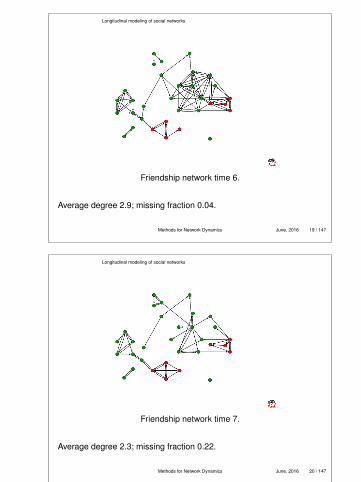
Friendship network time 6.
Average degree 2.9; missing fraction 0.04.
Methods for Network Dynamics June, 2016 19 / 147
Longitudinal modeling of social networks
Friendship network time 7.
Average degree 2.3; missing fraction 0.22.
Methods for Network Dynamics June, 2016 20 / 147
Longitudinal modeling of social networks
Which conclusions can be drawn from such a data set?
Dynamics of social networks are complicatedbecause “network effects” are endogenous feedback effects:e.g., reciprocity, transitivity, popularity, subgroup formation.
For statistical inference, we need models for network dynamicsthat are flexible enough to representthe complicated dependencies in such processes;while satisfying also the usual statistical requirementof parsimonious modelling:complicated enough to be realistic,not more complicated than empirically necessary and justifiable.
Methods for Network Dynamics June, 2016 21 / 147
Longitudinal modeling of social networks
For a correct interpretation of empirical observationsabout network dynamics collected in a panel design,it is crucial to consider a model with latent change going onbetween the observation moments.
E.g., groups may be regarded as the result of the coalescenceof relational dyads helped by a process of transitivity(“friends of my friends are my friends”).Which groups form may be contingent on unimportant details;that groups will form is a sociological regularity.
Therefore:use dynamic models with continuous time parameter:time runs on between observation moments.
Methods for Network Dynamics June, 2016 22 / 147
Longitudinal modeling of social networks
An advantage of using continuous-time models,even if observations are made at a few discrete time points,is that a more natural and simple representation may be found,especially in view of the endogenous dynamics.(cf. Coleman, 1964).
No problem with irregularly spaced data.
This has been done in a variety of models:
For discrete data: cf. Kalbfleisch & Lawless, JASA, 1985;for continuous data:mixed state space modelling well-known in engineering,in economics e.g. Bergstrom (1976, 1988),in social science Tuma & Hannan (1984), Singer (1990s).
Methods for Network Dynamics June, 2016 23 / 147
Longitudinal modeling of social networks
Purpose of statistical inference:investigate network evolution (dependent var.) as function of
simultaneously.By controlling adequately for structural effects, it is possibleto test hypothesized effects of variables on network dynamics(without such control these tests would be incomplete).
The structural effects imply that the presence of tiesis highly dependent on the presence of other ties.
Methods for Network Dynamics June, 2016 24 / 147
Longitudinal modeling of social networks
Principles for this approachto analysis of network dynamics:
1. use simulation models as models for data
2. comprise a random influence in the simulation modelto account for ‘unexplained variability’
3. use methods of statistical inferencefor probability models implemented as simulation models
4. for panel data: employ a continuous-time modelto represent unobserved endogenous network evolution
5. condition on the first observation and do not model it:no stationarity assumption.
Methods for Network Dynamics June, 2016 25 / 147
Longitudinal modeling of social networks
Stochastic Actor-Oriented Model (‘SAOM’)
1. Actors i = 1, . . . ,n (individuals in the network),pattern X of ties between them : one binary network X ;Xij = 0, or 1 if there is no tie, or a tie, from i to j .Matrix X is adjacency matrix of digraph.Xij is a tie indicator or tie variable.
2. Exogenously determined independent variables:actor-dependent covariates v , dyadic covariates w .These can be constant or changing over time.
3. Continuous time parameter t ,observation moments t1, . . . , tM .
4. Current state of network X (t) is dynamic constraint for its ownchange process: Markov process.
Methods for Network Dynamics June, 2016 26 / 147
Longitudinal modeling of social networks
‘actor-oriented’ = ‘actor-based’
5. The actors control their outgoing ties.
6. The ties have inertia: they are states rather than events.At any single moment in time,only one variable Xij(t) may change.
7. Changes are modeled aschoices by actors in their outgoing ties,with probabilities depending on ‘objective function’of the network state that would obtain after this change.
Methods for Network Dynamics June, 2016 27 / 147
Longitudinal modeling of social networks
The change probabilities can (but need not)be interpreted as arising from goal-directed behavior,in the weak sense of myopic stochastic optimization.
Assessment of the situation is represented byobjective function, interpreted as‘that which the actors seem to strive after in the short run’.
Next to actor-driven models,also tie-driven models are possible.
Methods for Network Dynamics June, 2016 28 / 147
Longitudinal modeling of social networks
At any given moment, with a given current network structure,the actors act independently, without coordination.They also act one-at-a-time.
The subsequent changes (‘micro-steps’) generatean endogenous dynamic contextwhich implies a dependence between the actors over time;e.g., through reciprocation or transitive closureone tie may lead to another one.
This implies strong dependence between what the actors do,but it is completely generated by the time order:the actors are dependent because they constituteeach other’s changing environment.
Methods for Network Dynamics June, 2016 29 / 147
Longitudinal modeling of social networks
The change process is decomposed into two sub-models,formulated on the basis of the idea that the actors i controltheir outgoing ties (Xi1, . . . ,Xin):
1. waiting times until the next opportunityfor a change made by actor i :rate functions;
2. probabilities of changing (toggling) Xij ,conditional on such an opportunity for change:objective functions.
The distinction between rate function and objective functionseparates the model for how many changes are madefrom the model for which changes are made.
Methods for Network Dynamics June, 2016 30 / 147
Longitudinal modeling of social networks
This decomposition between the timing model and themodel for change can be pictured as follows:
At randomly determined moments t ,actors i have opportunity to change a tie variable Xij :
micro step.(Actors are also permitted to leave things unchanged.)Frequency of micro steps is determined by rate functions.
When a micro step is taken,the probability distribution of the result of this stepdepends on the objective function :higher probabilities of moving toward new statesthat have higher values of the objective function.
Methods for Network Dynamics June, 2016 31 / 147
Longitudinal modeling of social networks
Specification: rate function
‘how fast is change / opportunity for change ?’
Rate of change of the network by actor i is denoted λi :expected frequency of opportunities for change by actor i .
Simple specification: rate functions are constant within periods.
More generally, rate functions can depend on observation period(tm−1, tm), actor covariates, network position (degrees etc.), throughan exponential link function.
Formally, for a certain short time interval (t , t + ε),the probability that this actor randomly gets an opportunityto change one of his/her outgoing ties, is given by ε λi .
Methods for Network Dynamics June, 2016 32 / 147
Longitudinal modeling of social networks
Specification: objective function
‘what is the direction of change?’
The objective function fi(β, x) indicatespreferred ‘directions’ of change.β is a statistical parameter, i is the actor (node), x the network.
When actor i gets an opportunity for change,he has the possibility to change one outgoing tie variable Xij ,or leave everything unchanged.
By x (±ij) is denoted the network obtainedwhen xij is changed (‘toggled’) into 1− xij .Formally, x (±ii) is defined to be equal to x .
Methods for Network Dynamics June, 2016 33 / 147
Longitudinal modeling of social networks
Conditional on actor i being allowed to make a change,the probability that Xij changes into 1− Xij is
pij(β, x) =exp
(fi(β, x (±ij))
)n∑
h=1
exp(fi(β, x (±ih))
) ,
and pii is the probability of not changing anything.
Higher values of the objective function indicatethe preferred direction of changes.
Methods for Network Dynamics June, 2016 34 / 147
Longitudinal modeling of social networks
One way of obtaining this model specification is to supposethat actors make changes such as to optimizethe objective function fi(β, x)
plus a random disturbance that has a Gumbel distribution,like in random utility models in econometrics:
(with the formal definition x (±ii) = x).Methods for Network Dynamics June, 2016 35 / 147
Longitudinal modeling of social networks
For a convenient distributional assumption,(U has type 1 extreme value = Gumbel distribution)
given that i is allowed to make a change,the probability that i changes the tie variable to j ,or leaves the tie variables unchanged (denoted by j = i), is
pij(β, x) =exp
(f (i , j)
)n∑
h=1
exp(f (i ,h)
)where
f (i , j) = fi(β, x (±ij))
and pii is the probability of not changing anything.
This is the multinomial logit form of a random utility model.
Methods for Network Dynamics June, 2016 36 / 147
Longitudinal modeling of social networks
Objective functions will be defined as sum of:
1. evaluation function expressing satisfaction with network;To allow asymmetry creation↔ termination of ties:
2. creation functionexpressing aspects of network structureplaying a role only for creating new ties
3. maintenance = endowment functionexpressing aspects of network structureplaying a role only for maintaining existing ties
If creation function = maintenance function,then these can be jointly replaced by the evaluation function.This is usual for starting modelling.
Methods for Network Dynamics June, 2016 37 / 147
Longitudinal modeling of social networks
Evaluation, creation, and maintenance functions are modeled aslinear combinations of theoretically argued componentsof preferred directions of change. The weights in the linearcombination are the statistical parameters.
This is a linear predictor like in generalized linear modeling(generalization of regression analysis).
Formally, the SAOM is a generalized statistical modelwith missing data (the microsteps are not observed).
The focus of modeling is first on the evaluation function;then on the rate and creation – maintenance functions.
Methods for Network Dynamics June, 2016 38 / 147
Longitudinal modeling of social networks
The objective function does not reflect the eventual ’utility’of the situation to the actor, but short-time goalsfollowing from preferences, constraints, opportunities.
The evaluation, creation, and maintenance functions expresshow the dynamics of the network processdepends on its current state.
Methods for Network Dynamics June, 2016 39 / 147
Longitudinal modeling of social networks
Stochastic process formulation
This specification implies that X follows acontinuous-time Markov chain with intensity matrix
qij(x) = limdt ↓ 0
P{
X (t + dt) = x (±ij) | X (t) = x}
dt(i 6= j)
given byqij(x) = λi(α, ρ, x) pij(β, x) .
Methods for Network Dynamics June, 2016 40 / 147
Longitudinal modeling of social networks
Computer simulation algorithmfor arbitrary rate function λi(α, ρ, x)
1. Set t = 0 and x = X (0).
2. Generate S according to theexponential distribution with mean 1/λ+(α, ρ, x) where
λ+(α, ρ, x) =∑
i
λi(α, ρ, x) .
3. Select i ∈ {1, ...,n} using probabilities
λi(α, ρ, x)
λ+(α, ρ, x).
Methods for Network Dynamics June, 2016 41 / 147
Longitudinal modeling of social networks
4. Select j ∈ {1, ...,n}, j 6= i using probabilities pij(β, x).
5. Set t = t + S and x = x (±ij).
6. Go to step 2(unless stopping criterion is satisfied).
Note that the change probabilities depend always onthe current network state, not on the last observed state!
Methods for Network Dynamics June, 2016 42 / 147
Longitudinal modeling of social networks
Model specification :Simple specification: only evaluation function;no separate creation or maintenance function,periodwise constant rate function.
Evaluation function fi reflects network effects(endogenous) and covariate effects (exogenous).Covariates can be actor-dependentor dyad-dependent.
Convenient definition of evaluation function is a weighted sum
fi(β, x) =L∑
k=1
βk sik (x) ,
where the weights βk are statistical parameters indicatingstrength of effect sik (x) (‘linear predictor’).
Methods for Network Dynamics June, 2016 43 / 147
Longitudinal modeling of social networks
Choose possible network effects for actor i , e.g.:(others to whom actor i is tied are called here i ’s ‘friends’)
1. out-degree effect, controlling the density / average degree,si1(x) = xi+ =
∑j xij
2. reciprocity effect, number of reciprocated tiessi2(x) =
∑j xij xji
Methods for Network Dynamics June, 2016 44 / 147
Longitudinal modeling of social networks
Various potential effects representing network closure:
3. transitive triplets effect (‘transTrip’),number of transitive patterns in i ’s ties(i → j , i → h, h→ j)si3(x) =
∑j,h xij xih xhj
i
h
j
transitive triplet4. transitive ties effect (‘transTies’),
number of actors j to whom i is tied indirectly(through at least one intermediary: xih = xhj = 1 )and also directly xij = 1),si4(x) = #{j | xij = 1, maxh(xih xhj) > 0}
Methods for Network Dynamics June, 2016 45 / 147
Longitudinal modeling of social networks
5. geometrically weighted edgewise shared partners(‘GWESP’; cf. ERGM)is intermediate between transTrip and transTies.
GWESP(i , α) =∑
j
xij eα{
1 −(1− e−α
)∑h xihxhj
}.
for α ≥ 0 (effect parameter = 100× α).Effect parameters are fixed parameters in an effect,allowing the user to choosebetween different versions of an effect.Default here: α = ln(2) ≈ 0.69,effect parameter = 69.
Methods for Network Dynamics June, 2016 46 / 147
Longitudinal modeling of social networks
GWESP is intermediate between transitive triplets (α =∞)and transitive ties (α = 0).
0 1 2 3 4 5 6
0
2
4
6
s
GW
ES
Pw
eigh
tα =∞α = 1.2α = 0.69α = 0
Weight of tie i → j for s =∑
h xihxhj two-paths.
Methods for Network Dynamics June, 2016 47 / 147
Longitudinal modeling of social networks
Differences between network closure effects:
I transitive triplets effect: i more attracted to jif there are more indirect ties i → h→ j ;
I transitive ties effect: i more attracted to jif there is at least one such indirect connection ;
I gwesp effect: in between these two;
I balance or Jaccard similarity effects (see manual):i prefers others j who make same choices as i .
Non-formalized theories usually do not distinguishbetween these different closure effects.It is possible to ’let the data speak for themselves’ and seewhat is the best formal representation of closure effects.
Methods for Network Dynamics June, 2016 48 / 147
Longitudinal modeling of social networks
6. three-cycle effect,number of three-cycles in i ’s ties(i → j , j → h, h→ i)si6(x) =
∑j,h xij xjh xhi
i
h
j
three-cycle
This represents a kind of generalized reciprocity,and absence of hierarchy.
Methods for Network Dynamics June, 2016 49 / 147
Longitudinal modeling of social networks
7. reciprocity × transitive triplets effect,number of triplets in i ’s tiescombining reciprocity and transitivity asfollows(i ↔ j , j → h, h→ i)si7(x) =
∑j,h xij xji xjh xhi
i
h
j
reciprocity ×trans. triplet
Simultaneous occurrence ofreciprocity and network closure(see Per Block, Social Networks, 2015.)
Methods for Network Dynamics June, 2016 50 / 147
Longitudinal modeling of social networks
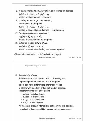
8. in-degree related popularity effect, sum friends’ in-degreessi8(x) =
∑j xij x+j =
∑j xij∑
h xhj
related to dispersion of in-degrees
9. out-degree related popularity effect,sum friends’ out-degreessi9(x) =
∑j xij xj+ =
∑j xij∑
h xjh
related to association in-degrees — out-degrees;
10. Outdegree-related activity effect ,si10(x) =
∑j xij xi+ = x2
i+
related to dispersion of out-degrees;
11. Indegree-related activity effect ,si11(x) =
∑j xij x+i = xi+ x+i
related to association in-degrees — out-degrees;
(These effects can also be defined with a √ sign.)Methods for Network Dynamics June, 2016 51 / 147
Longitudinal modeling of social networks
12. Assortativity effects:Preferences of actors dependent on their degrees.Depending on their own out- and in-degrees,actors can have differential preferences for tiesto others with also high or low out- and in-degrees.Together this yields 4 possibilities:
I out ego - out alter degreesI out ego - in alter degreesI in ego - out alter degreesI in ego - in alter degrees
All these are product interactions between the two degrees.Here also the degrees could be replaced by their square roots.
Methods for Network Dynamics June, 2016 52 / 147
Longitudinal modeling of social networks
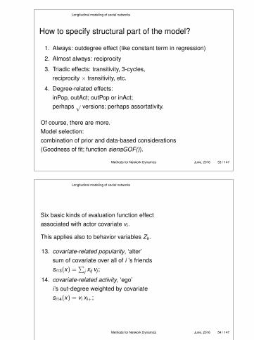
How to specify structural part of the model?
1. Always: outdegree effect (like constant term in regression)
2. Almost always: reciprocity
3. Triadic effects: transitivity, 3-cycles,reciprocity × transitivity, etc.
Evaluation function effect for dyadic covariate wij :
19. covariate-related preference,sum of covariate over all of i ’s friends,i.e., values of wij summed over all others to whom i is tied,si19(x) =
∑j xij wij .
If this has a positive effect, then the value of a tie i → jbecomes higher when wij becomes higher.
Methods for Network Dynamics June, 2016 57 / 147
Longitudinal modeling of social networks
Example
Data collected by Gerhard van de Bunt:group of 32 university freshmen,24 female and 8 male students.
Three observations used here (t1, t2, t3) :at 6, 9, and 12 weeks after the start of the university year.The relation is defined as a ‘friendly relation’.
Missing entries xij(tm) set to 0and not used in calculations of statistics.
Densities increase from 0.15 at t1 via 0.18 to 0.22 at t3 .
Methods for Network Dynamics June, 2016 58 / 147
Longitudinal modeling of social networks
Very simple model: only out-degree and reciprocity effects
Model 1
Effect par. (s.e.)
Rate t1 − t2 3.51 (0.54)Rate t2 − t3 3.09 (0.49)
Out-degree −1.10 (0.15)Reciprocity 1.79 (0.27)
rate parameters:per actor about 3 opportunities for change between observations;
out-degree parameter negative:on average, cost of friendship ties higher than their benefits;
This expresses ‘how much actor i likes the network’.
Adding a reciprocated tie (i.e., for which xji = 1) gives
−1.10 + 1.79 = 0.69.
Adding a non-reciprocated tie (i.e., for which xji = 0) gives
−1.10,
i.e., this has negative benefits.Gumbel distributed disturbances are added:these have variance π2/6 = 1.645 and s.d. 1.28.
Methods for Network Dynamics June, 2016 60 / 147
Longitudinal modeling of social networks
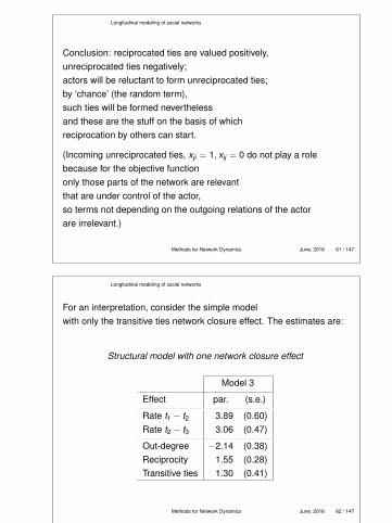
Conclusion: reciprocated ties are valued positively,unreciprocated ties negatively;actors will be reluctant to form unreciprocated ties;by ‘chance’ (the random term),such ties will be formed neverthelessand these are the stuff on the basis of whichreciprocation by others can start.
(Incoming unreciprocated ties, xji = 1, xij = 0 do not play a rolebecause for the objective functiononly those parts of the network are relevantthat are under control of the actor,so terms not depending on the outgoing relations of the actorare irrelevant.)
Methods for Network Dynamics June, 2016 61 / 147
Longitudinal modeling of social networks
For an interpretation, consider the simple modelwith only the transitive ties network closure effect. The estimates are:
Structural model with one network closure effect
Model 3
Effect par. (s.e.)
Rate t1 − t2 3.89 (0.60)Rate t2 − t3 3.06 (0.47)
Out-degree −2.14 (0.38)Reciprocity 1.55 (0.28)Transitive ties 1.30 (0.41)
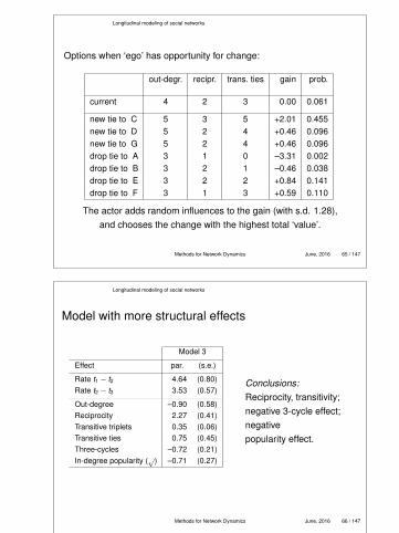
new tie to C 5 3 5 +2.01 0.455new tie to D 5 2 4 +0.46 0.096new tie to G 5 2 4 +0.46 0.096drop tie to A 3 1 0 –3.31 0.002drop tie to B 3 2 1 –0.46 0.038drop tie to E 3 2 2 +0.84 0.141drop tie to F 3 1 3 +0.59 0.110
The actor adds random influences to the gain (with s.d. 1.28),and chooses the change with the highest total ‘value’.
Conclusions:Trans. ties nownot needed any moreto representtransitivity;men more popular;program similarity.
Methods for Network Dynamics June, 2016 67 / 147
Longitudinal modeling of social networks
To interpret the three effects of actor covariate gender,it is more instructive to consider them simultaneously.Gender was coded originally by with 1 for F and 2 for M.This dummy variable was centered (mean was subtracted)but this only adds a constant to the values presented next,and does not affect the differences between them.
Therefore we may do the calculations with F = 0, M = 1.
Methods for Network Dynamics June, 2016 68 / 147
Longitudinal modeling of social networks
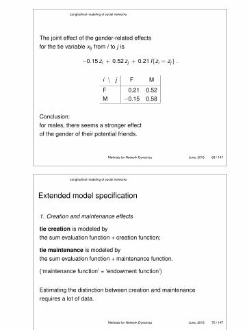
The joint effect of the gender-related effectsfor the tie variable xij from i to j is
−0.15 zi + 0.52 zj + 0.21 I{zi = zj} .
i \ j F M
F 0.21 0.52M −0.15 0.58
Conclusion:for males, there seems a stronger effectof the gender of their potential friends.
Methods for Network Dynamics June, 2016 69 / 147
Longitudinal modeling of social networks
Extended model specification
1. Creation and maintenance effects
tie creation is modeled bythe sum evaluation function + creation function;
tie maintenance is modeled bythe sum evaluation function + maintenance function.
(‘maintenance function’ = ‘endowment function’)
Estimating the distinction between creation and maintenancerequires a lot of data.
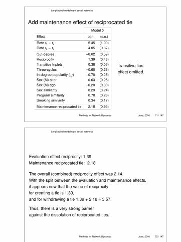
The overall (combined) reciprocity effect was 2.14.With the split between the evaluation and maintenance effects,it appears now that the value of reciprocityfor creating a tie is 1.39,and for withdrawing a tie 1.39 + 2.18 = 3.57.
Thus, there is a very strong barrieragainst the dissolution of reciprocated ties.
Methods for Network Dynamics June, 2016 72 / 147
Longitudinal modeling of social networks
Extended model specification
2. Non-constant rate function λi(α, ρ, x) .
This means that some actors change their tiesmore quickly than others,depending on covariates or network position.
Dependence on covariates:
λi(α, ρ, x) = ρm exp(∑
h
αh vhi) .
ρm is a period-dependent base rate.
(Rate function must be positive; ⇒ exponential function.)
Methods for Network Dynamics June, 2016 73 / 147
Longitudinal modeling of social networks
Dependence on network position:e.g., dependence on out-degrees:
λi(α, ρ, x) = ρm exp(α1 xi+) .
Also, in-degrees and ] reciprocated ties of actor imay be used.
Now the parameter is θ = (ρ, α, β, γ).
Methods for Network Dynamics June, 2016 74 / 147
Longitudinal modeling of social networks
Continuation example
Rate function depends on out-degree:those with higher out-degreesalso change their tie patterns more quickly.
maintenance function depends on tie reciprocationReciprocity operates differentlyfor tie initiation than for tie withdrawal.
Methods for Network Dynamics June, 2016 75 / 147
Longitudinal modeling of social networks
Parameter estimates model with rate and maintenance effects
non-significant tendency that actors with higher out-degreeschange their ties more often (t = 0.041/0.034 = 1.2),
value of reciprocation is larger for termination of tiesthan for creation (t = 1.82/0.97 = 1.88).
Methods for Network Dynamics June, 2016 77 / 147
Longitudinal modeling of social networks
Non-directed networks
The actor-driven modeling is less straightforwardfor non-directed relations,because two actors are involved in deciding about a tie.
Various modeling options are possible:
1. Forcing model:one actor takes the initiative and unilaterally imposesthat a tie is created or dissolved.
Methods for Network Dynamics June, 2016 78 / 147
Longitudinal modeling of social networks
2. Unilateral initiative with reciprocal confirmation:one actor takes the initiative and proposes a new tieor dissolves an existing tie;if the actor proposes a new tie, the other has to confirm,otherwise the tie is not created.
3. Pairwise conjunctive model:a pair of actors is chosen and reconsider whether a tiewill exist between them; a new tie is formed if both agree.
4. Pairwise disjunctive (forcing) model:a pair of actors is chosen and reconsider whether a tiewill exist between them;a new tie is formed if at least one wishes this.
Methods for Network Dynamics June, 2016 79 / 147
Longitudinal modeling of social networks
5. Pairwise compensatory (additive) model:a pair of actors is chosen and reconsider whether a tiewill exist between them; this is basedon the sum of their utilities for the existence of this tie.
Option 1 is close to the actor-driven model for directed relations.
In options 3–5, the pair of actors (i , j) is chosendepending on the product of the rate functions λi λj
(under the constraint that i 6= j ).
The numerical interpretation of the ratio functiondiffers between options 1–2 compared to 3–5.
The decision about the tie is taken on the basis of the objectivefunctions fi fj of both actors.
Methods for Network Dynamics June, 2016 80 / 147
Estimation
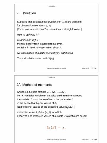
2. Estimation
Suppose that at least 2 observations on X (t) are available,for observation moments t1, t2.(Extension to more than 2 observations is straightforward.)
How to estimate θ?
Condition on X (t1) :the first observation is accepted as given,contains in itself no observation about θ.
No assumption of a stationary network distribution.
Thus, simulations start with X (t1).
Methods for Network Dynamics June, 2016 81 / 147
Estimation
2A. Method of moments
Choose a suitable statistic Z = (Z1, . . . ,ZK ),i.e., K variables which can be calculated from the network;the statistic Z must be sensitive to the parameter θin the sense that higher values of θk
lead to higher values of the expected value Eθ(Zk ) ;
determine value θ̂ of θ = (ρ, β) for whichobserved and expected values of suitable Z statistic are equal:
Eθ̂ {Z} = z .
Methods for Network Dynamics June, 2016 82 / 147
Estimation
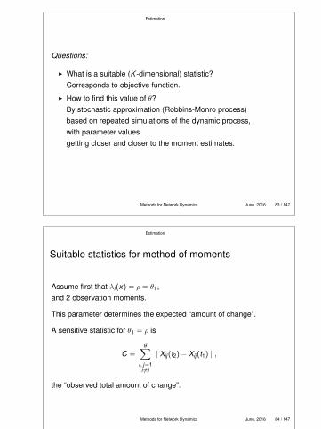
Questions:
I What is a suitable (K -dimensional) statistic?Corresponds to objective function.
I How to find this value of θ?By stochastic approximation (Robbins-Monro process)based on repeated simulations of the dynamic process,with parameter valuesgetting closer and closer to the moment estimates.
Methods for Network Dynamics June, 2016 83 / 147
Estimation
Suitable statistics for method of moments
Assume first that λi(x) = ρ = θ1,and 2 observation moments.
This parameter determines the expected “amount of change”.
A sensitive statistic for θ1 = ρ is
C =
g∑i, j=1i 6=j
| Xij(t2)− Xij(t1) | ,
the “observed total amount of change”.
Methods for Network Dynamics June, 2016 84 / 147
Estimation
For the weights βk in the evaluation function
fi(β, x) =L∑
k=1
βk sik (x) ,
a higher value of βk means that all actorsstrive more strongly after a high value of sik (x),so sik (x) will tend to be higher for all i , k .
This leads to the statistic
Sk =n∑
i=1
sik (X (t2)) .
This statistic will be sensitive to βk :a high βk will to lead to high values of Sk .
Methods for Network Dynamics June, 2016 85 / 147
Estimation
Moment estimation will be based on thevector of statistics
Z = (C,S1, ...,SK−1) .
Denote by z the observed value for Z .The moment estimate θ̂ is defined as the parameter valuefor which the expected value of the statisticis equal to the observed value:
Eθ̂{Z} = z .
Methods for Network Dynamics June, 2016 86 / 147
Estimation
Robbins-Monro algorithm
The moment equation Eθ̂{Z} = z cannot be solved byanalytical or the usual numerical procedures, because
Eθ{Z}
cannot be calculated explicitly.
However, the solution can be approximated by theRobbins-Monro (1951) method for stochastic approximation.
Iteration step:θ̂N+1 = θ̂N − aN D−1(zN − z) , (1)
where zN is a simulation of Z with parameter θ̂N ,D is a suitable matrix, and aN → 0 .
Methods for Network Dynamics June, 2016 87 / 147
Estimation
Covariance matrix
The method of moments yields the covariance matrix
cov(θ̂) ≈ D−1θ Σθ D′θ
−1
where
Σθ = cov{Z |X (t1) = x(t1)}
Dθ =∂
∂θE{Z |X (t1) = x(t1)} .
Matrices Σθ and Dθ can be estimatedfrom MC simulations with fixed θ.
Methods for Network Dynamics June, 2016 88 / 147
Estimation
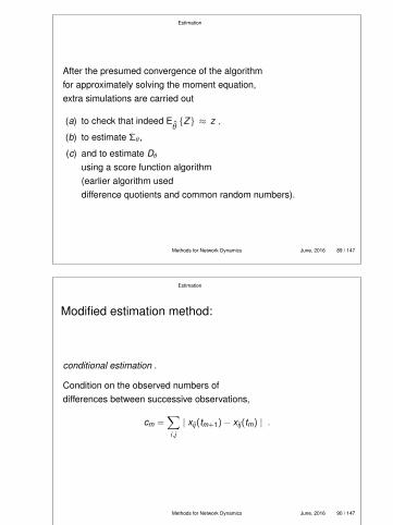
After the presumed convergence of the algorithmfor approximately solving the moment equation,extra simulations are carried out
(a) to check that indeed Eθ̂{Z} ≈ z ,
(b) to estimate Σθ,
(c) and to estimate Dθ
using a score function algorithm(earlier algorithm useddifference quotients and common random numbers).
Methods for Network Dynamics June, 2016 89 / 147
Estimation
Modified estimation method:
conditional estimation .
Condition on the observed numbers ofdifferences between successive observations,
cm =∑i,j
| xij(tm+1)− xij(tm) | .
Methods for Network Dynamics June, 2016 90 / 147
Estimation
For continuing the simulations do not mind the values ofthe time variable t ,but continue between tm and tm+1 untilthe observed number of differences∑
i,j
| Xij(t)− xij(tm) |
is equal to the observed cm .This is defined as time moment tm+1 .
This procedure is a bit more stable;requires modified estimator of ρm .
Methods for Network Dynamics June, 2016 91 / 147
Estimation
Computer algorithm has 3 phases:
1. brief phase for preliminary estimation of ∂Eθ {Z}/∂θfor defining D;
2. estimation phase with Robbins-Monro updates,where aN remains constant in subphasesand decreases between subphases;
3. final phase where θ remains constant at estimated value;this phase is for checking that
Eθ̂{Z} ≈ z ,
and for estimating Dθ and Σθ to calculate standard errors.
Methods for Network Dynamics June, 2016 92 / 147
Estimation
Extension: more periods
The estimation method can be extendedto more than 2 repeated observations:observations x(t) for t = t1, ..., tM .
Parameters remain the same in periods between observationsexcept for the basic rate of change ρwhich now is given by ρm for tm ≤ t < tm+1 .
For the simulations,the simulated network X (t) is reset to the observation x(tm)
whenever the time parameter t passes the observation time tm .
The statistics for the method of moments are defined assums of appropriate statistics calculated per period (tm, tm+1).
Methods for Network Dynamics June, 2016 93 / 147
Estimation
The procedures are implemented in the R package
R
S imulation
I nvestigation forE mpiricalN etworkA nalysis
(frequently updated) with the website
http://www.stats.ox.ac.uk/siena/.
(programmed by Tom Snijders, Ruth Ripley, Krists Boitmanis;contributions by many others).
Methods for Network Dynamics June, 2016 94 / 147
Dynamics of networks and behavior
3. Networks as dependent and independent variables
Co-evolution
Simultaneous endogenous dynamics of networks and behavior: e.g.,
I individual humans & friendship relations:attitudes, behavior (lifestyle, health, etc.)
I individual humans & cooperation relations:work performance
I companies / organisations & alliances, cooperation:performance, organisational success.
Methods for Network Dynamics June, 2016 95 / 147
Dynamics of networks and behavior
Two-way influence between networks and behavior
Relational embeddedness is importantfor well-being, opportunities, etc.
Actors are influenced in their behavior, attitudes, performanceby other actors to whom they are tiede.g., network resources (social capital), social control.
(N. Friedkin, A Structural Theory of Social Influence, C.U.P., 1998).
Methods for Network Dynamics June, 2016 96 / 147
Dynamics of networks and behavior
In return, many types of tie(friendship, cooperation, liking, etc.)are influenced positively bysimilarity on relevant attributes: homophily(e.g., McPherson, Smith-Lovin, & Cook, Ann. Rev. Soc., 2001.)
More generally, actors choose relation partnerson the basis of their behavior and other characteristics(similarity, opportunities for future rewards, etc.).
Influence, network & behavior effects on behavior;Selection, network & behavior effects on relations.
Methods for Network Dynamics June, 2016 97 / 147
Dynamics of networks and behavior
Terminology
relation = network = pattern of ties in group of actors;behavior = any individual-bound changeable attribute
(including attitudes, performance, etc.).
Relations and behaviors are endogenous variablesthat develop in a simultaneous dynamics.
Thus, there is a feedback relation in the dynamicsof relational networks and actor behavior / performance:macro⇒ micro⇒ macro · · · ·
(although network perhaps is meso rather than macro)
Methods for Network Dynamics June, 2016 98 / 147
Dynamics of networks and behavior
The investigation of such social feedback processes is difficult:
I Both the network⇒ behaviorand the behavior⇒ network effectslead ‘network autocorrelation’:“friends of smokers are smokers”“high-reputation firms don’t collaboratewith low-reputation firms”.It is hard to ascertain the strengthsof the causal relations in the two directions.
I For many phenomenaquasi-continuous longitudinal observation is infeasible.Instead, it may be possible to observenetworks and behaviors at a few discrete time points.
Methods for Network Dynamics June, 2016 99 / 147
Dynamics of networks and behavior
Data
One bounded set of actors(e.g. school class, group of professionals, set of firms);
Integrate the influence (dep. var. = behavior)and selection (dep. var. = network) processes.
In addition to the network X , associated to each actor ithere is a vector Zi(t) of actor characteristicsindexed by h = 1, . . . , H.Assumption: ordered discrete(simplest case: one dichotomous variable).
Methods for Network Dynamics June, 2016 101 / 147
Dynamics of networks and behavior
Actor-driven models
Each actor “controls” not only his outgoing ties,collected in the row vector
(Xi1(t), ...,Xin(t)
),
but also his behavior Zi(t) =(
Zi1(t), ...,ZiH(t))
(H is the number of dependent behavior variables).
Network change process and behavior change processrun simultaneously, and influence each otherbeing each other’s changing constraints.
Methods for Network Dynamics June, 2016 102 / 147
Dynamics of networks and behavior
At stochastic times(rate functions λX for changes in network,λZh for changes in behavior h),the actors may change a tie or a behavior.
Probabilities of change are increasing functions ofobjective functions of the new state,defined specifically for network, f X ,and for behavior, f Z .
Again, only the smallest possible steps are allowed:change one tie variable,or move one step up or down on a behavior variable.
Methods for Network Dynamics June, 2016 103 / 147
Dynamics of networks and behavior
For network change, change probabilities are as before.
For the behaviors, the formula of the change probabilities is
pihv (β, z) =exp(f (i ,h, v))∑
k ,u
exp(f (i , k ,u))
where f (i ,h, v) is the objective function calculated for the potential newsituation after a behavior change,
f (i ,h, v) = f Zi (β, z(i ,h ; v)) .
Again, multinomial logit form.
Again, a ‘maximizing’ interpretation is possible.
Methods for Network Dynamics June, 2016 104 / 147
Dynamics of networks and behavior
Micro-step for change in network:
At random moments occurring at a rate λXi ,
actor i is designatedto make a change in one tie variable:the micro-step (on⇒ off, or off⇒ on.)
micro-step for change in behavior:
At random moments occurring at a rate λZhi ,
actor i is designated to make a change in behavior h(one component of Zi , assumed to be ordinal):the micro-step is a change to an adjacent category.
Again, many micro-steps can accumulate to big differences.
Methods for Network Dynamics June, 2016 105 / 147
Dynamics of networks and behavior
Optimizing interpretation:
When actor i ‘may’ change an outgoing tie variable to some other actorj , he/she chooses the ’best’ j by maximizingthe evaluation function f X
i (β,X , z) of the situation obtainedafter the coming network changeplus a random component representing unexplained influences;
and when this actor ‘may’ change behavior h,he/she chooses the “best” change (up, down, nothing)by maximizing the evaluation function f Zh
i (β, x ,Z ) of the situationobtained after the coming behavior changeplus a random component representing unexplained influences.
Methods for Network Dynamics June, 2016 106 / 147
Dynamics of networks and behavior
Optimal network change:
The new network is denoted by x (±ij).The attractiveness of the new situation(evaluation function plus random term)is expressed by the formula
f Xi (β, x (±ij), z) + UX
i (t , x , j) .
⇑
random component
(Note that the network is also permitted to stay the same.)
Methods for Network Dynamics June, 2016 107 / 147
Dynamics of networks and behavior
Optimal behavior change:
Whenever actor i may make a change in variable h of Z ,he changes only one behavior, say zih , to the new value v .The new vector is denoted by z(i ,h ; v).Actor i chooses the “best” h, v by maximizing the objective function ofthe situation obtained after the coming behavior change plus a randomcomponent:
f Zhi (β, x , z(i ,h ; v)) + UZh
i (t , z,h, v) .
⇑
random component
(behavior is permitted to stay the same.)
Methods for Network Dynamics June, 2016 108 / 147
Dynamics of networks and behavior
Specification of the behavior model
Many different reasons why networksare important for behavior:
2. social capital :individuals may use resources of others;
3. coordination :individuals can achieve some goalsonly by concerted behavior;
Theoretical elaboration helpful for a good data analysis.
Methods for Network Dynamics June, 2016 109 / 147
Dynamics of networks and behavior
Basic effects for dynamics of behavior f Zi :
f Zi (β, x , z) =
L∑k=1
βk sik (x , z) ,
1. linear shape ,sZ
i1(x , z) = zih
2. quadratic shape, ‘effect behavior on itself’,sZ
i2(x , z) = z2ih
Quadratic shape effect important for model fit.
Methods for Network Dynamics June, 2016 110 / 147
Dynamics of networks and behavior
For a negative quadratic shape parameter,the model for behavior is a unimodal preference model.
zh
f Zhi (β, x, z)
1 2 3 4
For positive quadratic shape parameters ,the behavior objective function can be bimodal(‘positive feedback’).
Methods for Network Dynamics June, 2016 111 / 147
Dynamics of networks and behavior
3. behavior-related average similarity,average of behavior similarities between i and friendssi3(x) = 1
xi+
∑j xij sim(zih, zjh)
where sim(zih, zjh) is the similarity between vi and vj ,
sim(zih, zjh) = 1−|zih − zjh|
RZ h,
RZ h being the range of Z h;
4. average behavior alter — an alternative to similarity:si4(x , z) = zih
1xi+
∑j xijzjh
Effects 3 and 4 are alternatives for each other:they express the same theoretical idea of influencein mathematically different ways.The data will have to differentiate between them.
Methods for Network Dynamics June, 2016 112 / 147
Dynamics of networks and behavior
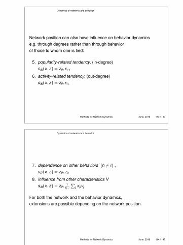
Network position can also have influence on behavior dynamicse.g. through degrees rather than through behaviorof those to whom one is tied:
7. dependence on other behaviors (h 6= `) ,si7(x , z) = zih zi`
8. influence from other characteristics Vsi8(x , z) = zih
1xi+
∑j xijvj
For both the network and the behavior dynamics,extensions are possible depending on the network position.
Methods for Network Dynamics June, 2016 114 / 147
Dynamics of networks and behavior
Now focus on the similarity effect in evaluation function :
sum of absolute behavior differences between i and his friendssi2(x , z) =
∑j xij sim(zih, zjh) .
This is fundamental bothto network selection based on behavior,and to behavior change based on network position.
Methods for Network Dynamics June, 2016 115 / 147
Dynamics of networks and behavior
A positive coefficient for this effect means that the actorsprefer friends with similar Zh values(network autocorrelation).
Actors can attempt to attain this by changing their ownZh value to the average value of their friends(network influence, contagion),
or by becoming friends with those with similar Zh values(selection on similarity).
Methods for Network Dynamics June, 2016 116 / 147
Dynamics of networks and behavior
Statistical estimation: networks & behavior
Procedures for estimating parameters in this model aresimilar to estimation procedures for network-only dynamics:Methods of Moments & Stochastic Approximation,conditioning on the first observation X (t1),Z (t1) .
The two different effects,networks⇒ behavior and behavior⇒ networks,both lead to network autocorrelation of behavior;
but they can be (in principle)distinguished empirically by the time order: respectivelyassociation between ties at tm and behavior at tm+1;and association between behavior at tm and ties at tm+1.
Methods for Network Dynamics June, 2016 117 / 147
Dynamics of networks and behavior
Statistics for use in method of moments:
for estimating parameters in network dynamics:
M−1∑m=1
n∑i=1
sik (X (tm+1),Z (tm)) ,
and for the behavior dynamics:
M−1∑m=1
n∑i=1
sik (X (tm),Z (tm+1)) .
Methods for Network Dynamics June, 2016 118 / 147
Dynamics of networks and behavior
The data requirements for these models are strong:few missing data; enough change on the behavioral variable.
Currently, work still is going on about good waysfor estimating parameters in these models.
Maximum likelihood estimation procedures(currently even more time-consuming; under construction...)are preferable for small data sets.
Methods for Network Dynamics June, 2016 119 / 147
Dynamics of networks and behavior
Example :Study of smoking initiation and friendship(following up on earlier work by P. West, M. Pearson & others)
One school year group from a Scottish secondary schoolstarting at age 12-13 years, was monitored over 3 years;total of 160 pupils, of which 129 pupils present at all 3 observations;with sociometric & behavior questionnaires at three moments, at appr.1 year intervals.
Smoking: values 1–3;drinking: values 1–5;
covariates:gender, smoking of parents and siblings (binary),money available (range 0–40 pounds/week).
Linear shape 0.44 (0.17)Quadratic shape –0.64 (0.22)Ave. alter 1.34 (0.61)Smoking 0.01 (0.21)Sex (F) 0.04 (0.22)Money 0.17 (0.16)Romantic experience –0.19 (0.27)
Methods for Network Dynamics June, 2016 131 / 147
Dynamics of networks and behavior
Conclusion:
In this case, the conclusions from a more elaborate model– i.e., with better control for alternative explanations –are similar to the conclusions from the simple model.
There is evidence for friendship selection based on drinking,and for social influence with respect to smoking and drinking.
Methods for Network Dynamics June, 2016 132 / 147
Dynamics of networks and behavior
Parameter interpretation for behavior change
Omitting the non-significant parameters yieldsthe following objective functions.For smoking
I These models represent network structureas well as attributes / behavior.
I Theoretically: they combine agency and structure.
I Available inpackage RSiena in the statistical system R.
I The method still is in a stage of development:extension to new data structures(e.g., multivariate, valued, larger networks),new procedures (goodness of fit),more experience with how to apply it.
Methods for Network Dynamics June, 2016 137 / 147
Dynamics of networks and behavior
Discussion (2)
I This approach attempts to tackle peer effects questionsby process modeling: data-intensiveand potentially assumption-intensive.Cox / Fisher: Make your theories elaborate.
I This type of analysis offers a very restrictedtake an causality:only time sequentiality.
I Assessing network effects is full of confounders.Careful theory development, good data are important.Asses goodness of fit of estimated model.
Methods for Network Dynamics June, 2016 138 / 147
Dynamics of networks and behavior
Co-evolution
The idea of ‘network-behaviour co-evolution’:
network is considered as one complex variable X (t);
behaviour is considered as one complex variable Z (t);
these are evolving over time in mutual dependence X (t)↔ Z (t),changes occurring in many little steps,where changes in X are a function of the current values of
(X (t),Z (t)
),
and the same holds for changes in Z .
This may be regarded as a ‘systems approach’,and is also applicable to more than one networkand more than one behavior.
Methods for Network Dynamics June, 2016 139 / 147
Dynamics of networks and behavior
Co-evolution of multiple networks
See Snijders – Lomi – Torló in Social Networks, 2013.
For example:
friendship and advice;
positive and negative ties.
Co-evolution of one-mode and two-mode networks:
e.g., friendship and shared activities,
Methods for Network Dynamics June, 2016 140 / 147
Conclusion
Why follow a statistical modeling approachto network analysis?
⇒ Combination of networks and attributesand: combination of structure and agency.
⇒ Distinction dependent⇔ explanatory variables
⇒ Hypothesis testing,clearer support of theory development.
⇒ Combination of multiple mechanisms: test theorieswhile controlling for alternative explanations.
⇒ Assessment of uncertainties in inference.
Methods for Network Dynamics June, 2016 141 / 147
Conclusion
Other work (recent, current, near future)
1. Changing composition of node set (Huisman & Snijders, SMR 2003),see manual.
2. Score-type tests (Schweinberger, BJMSP 2011).
3. Time heterogeneity (Lospinoso et al., ADAC 2011),function sienaTimeTest.
4. Goodness of fit (Lospinoso), function sienaGOF.
5. Random effects multilevel network models.New function sienaBayes() (Koskinen, Snijders)
6. Valued relations.
7. Larger networks, dropping assumption of complete information(Preciado)
8. Diffusion of innovations (Greenan)
Methods for Network Dynamics June, 2016 143 / 147
Conclusion
Some references about longitudinal models
I Tom A.B. Snijders,The Statistical Evaluation of Social Network Dynamics,Sociological Methodology 2001, 361–395;
I Tom A.B. Snijders, Models for Longitudinal Network Data, Ch. 11 in P.Carrington, J. Scott, & S. Wasserman (Eds.), Models and methods in socialnetwork analysis. New York: Cambridge University Press (2005).
I Tom A.B. Snijders, Gerhard G. van de Bunt, Christian E.G. Steglich (2010),Introduction to actor-based models for network dynamics. Social Networks, 32,44–60.
I See SIENA manual and homepage.
Methods for Network Dynamics June, 2016 144 / 147
Conclusion
Some references in various languages
I Ainhoa de Federico de la Rúa, L’Analyse Longitudinale de Réseaux sociaux totaux avecSIENA – Méthode, discussion et application.BMS, Bulletin de Méthodologie Sociologique, 84, October 2004, 5–39.
I Ainhoa de Federico de la Rúa, El análisis dinámico de redes sociales con SIENA. Método,Discusión y Aplicación.Empiria, 10, 151–181 (2005).
I Mark Huisman and Tom A.B. Snijders, Een stochastisch model voor netwerkevolutie.Nederlands Tijdschrift voor de Psychologie, 58 (2003), 182-194.
I Laura Savoia (2007), L’analisi della dinamica del network con SIENA.In: A. Salvini (a cura di), Analisi delle reti sociali. Teorie, metodi, applicazioni, Milano:FrancoAngeli.
I Christian Steglich and Andrea Knecht (2009), Die statistische Analyse dynamischerNetzwerkdaten.In: Christian Stegbauer and Roger Häußling (Hsrg.), Handbuch der Netzwerkforschung,Wiesbaden (Verlag für Sozialwissenschaften).
Methods for Network Dynamics June, 2016 145 / 147
Conclusion
Some references for dynamics of networks and behavior
I Tom Snijders, Christian Steglich, and Michael Schweinberger (2007),Modeling the co-evolution of networks and behavior.In: Longitudinal models in the behavioral and related sciences, eds. Kees van
Montfort, Han Oud and Albert Satorra; Lawrence Erlbaum, pp. 41–71.
I Steglich, C.E.G., Snijders, T.A.B. and Pearson, M. (2010).Dynamic Networks and Behavior: Separating Selection from Influence.Sociological Methodology, 329–393.
I René Veenstra, Jan Kornelis Dijkstra, Christian Steglich and Maarten H.W. Van Zalk (2013). Network-Behavior Dynamics.Journal of Research on Adolescence, 23, 399–412.
I Many articles with examples on Siena website.
Methods for Network Dynamics June, 2016 146 / 147
Conclusion
Further study – keeping updated
1. Note that the version of RSiena at CRAN is out of date;use the R-Forge version instead (see website - downloads).
2. Tom A.B. Snijders, Gerhard G. van de Bunt, Christian E.G.Steglich (2010), Introduction to actor-based models for networkdynamics. Social Networks, 32, 44–60.
3. The manual (available from website) has a lot of material.
4. Go through the website to see what’s there:http://www.stats.ox.ac.uk/siena/
5. There is also a user’s group:http://groups.yahoo.com/groups/stocnet/