Copyright 2009. StATS Ltd Pty Australia and Agro-Tech, Inc. USA. 1
Statistical modelling of a split-block agricultural field experiment.
*Mick O’Neill and Curtis J. Lee
Mick O’Neill, Statistical Advisory & Training Service Pty Ltd, NSW, Australia
Curt Lee, Agro-Tech, Inc., Velva, North Dakota, 58790
ABSTRACT
This is a statistical review of a split-block experiment used to evaluate the effect of
fungicides on modern and old spring wheat varieties historically grown in North Dakota. A
split-block experiment with random blocks has implications regarding the correlation
structures between plot yields in the field. These correlation structures are often unreasonable
for agricultural field trials. Considerations in the design and analysis of such an experiment
are discussed and an alternative approach to traditional analysis of variance (ANOVA) is
presented. A Linear Mixed Model (with uses a residual maximum likelihood algorithm) is
used to fit correlation structures to a row x column analysis and provide an improved
statistical model. REML provides a flexible and powerful analytical tool for fitting
complexities not handling by traditional ANOVA techniques.
ACKNOWLEDGMENT
The authors wish to thank Prof Roger Payne, Rothamsted Research, Harpenden,
Hertfordshire, UK for comments and suggestions that led to an improved paper.
KEY WORDS. Split-block, correlation structures, linear mixed models, residual maximum
likelihood, deviance, wheat, fungicide, row x column, agriculture, and field experiment.
* Email [email protected], web address www.stats.net.au
Copyright 2009. StATS Ltd Pty Australia and Agro-Tech, Inc. USA. 2
Statistical modelling of a split-block agricultural field experiment.
1. Background
An experiment was conducted as a preliminary evaluation of how spring wheat (Triticum
aestivum) varieties respond differently to the use of modern fungicide treatments, and to
determine if older wheat varieties would yield equally or better than currently grown lines
with the use of fungicides. Interest in old wheat varieties (sometimes referred to as heritage
wheats) has increased with a conservation movement to preserve wheat germplasm and
cultural cuisine. Heritage wheat line popularity has increased as entrepreneurs attempt to
develop niche markets in the wheat industry. Studies have claimed some possible advantages
to growing old wheats. This includes higher nutrient content, superior weed-crop
competition, and less need for inputs in sustainable type farming systems.
Hard red spring wheat varieties were planted near Velva, North Dakota, on April 28, 2007
and harvested on August 20, 2007. Wheat varieties were chosen based on historical
significance to the regional wheat industry and seed availability. The 16 varieties evaluated
are presented in Table 1. As the data set is only from one year and one environment, its
usefulness is limited to it original purpose.
Table 1. Spring wheat variety numbers (#), names and years of release.
# Name Year # Name Year # Name Year # Name Year
1 Red Fife† 1841 5 Len§ 1979 9 Grandin§ 1989 13 Alsen§ 2000
2 Marquis‡ 1901 6 Stoa§ 1984 10 2375# 1990 14 Steele-ND§ 2004
3 Waldron§ 1969 7 Butte 86§ 1986 11 Parshall§ 1999 15 Glenn§ 2005
4 Era 1970 8 Amidon§ 1988 12 Reeder§ 1999 16 Howard§ 2006
† = Canada
‡ = Dominion Department of Agriculture, Ottawa, Canada.
§ = North Dakota Agricultural Experiment Station
¶ = Minnesota Agricultural Experiment Stations
# = Pioneer Hi-Bred
Wheat has been selected for improved disease resistance throughout history. Consequently,
older varieties are normally more susceptible to fungal diseases as they have been replaced as
new strains occur and resistance is lost. New varieties are bred for increased disease
resistance to specific pathogens and are often adapted to specific production areas
(environments). So differences were expected as to (i) the diseases varieties are resistant to
and (ii) the level of resistance they have.
Copyright 2009. StATS Ltd Pty Australia and Agro-Tech, Inc. USA. 3
Statistical modelling of a split-block agricultural field experiment.
The varieties were randomized into three blocks using a randomized complete block design
(RCBD) for varieties. Plots in a block were contiguous, however to anticipate the application
of a fungicide treatment, each variety was sown in two sub-plots, each sub-plot being 5 ft
wide by 30 ft long with a 5 ft alley between them. Blocks were also contiguous with a 5 ft
alley between them. Plots were sprayed with Headline (pyraclostrobin, 3 oz/acre) at the 5 leaf
stage and with Folicur (tebuconazole, 4 oz/acre) at flowering. This fungicide treatment was
applied at random into half of each block, i.e. into the left or right sub-plot of each variety but
consistent (stripped) across the whole block – see Figure 1.
Figure 1 Site of field trial, with the randomized fungicide treatment indicated
Block 1
Block 2
Block 3
none
Fungicide
Fungicide
none
Fungicide
none
Plots were trimmed to an equal length before harvest and grain yield (t/ha) was calculated
based on 13% moisture content. The yield in t/ha is given in Table 2, along with the
randomization of varieties in the blocks. We have labelled the rows from 16 down to 1 to
allow residuals to be plotted in field order in subsequent analyses – one needs to imagine an
X-Y grid placed over the plots in the field, with a mathematical origin (0, 0) placed at the
bottom left corner plot. Then as one moves to the right from the origin towards the bottom
right corner plot the X coordinates on this grid system will be 1, 2, ..., 6, while moving up
from the origin towards the top left corner plot the Y coordinates will be 1, 2, ..., 16.
Copyright 2009. StATS Ltd Pty Australia and Agro-Tech, Inc. USA. 4
Statistical modelling of a split-block agricultural field experiment.
Table 2. Allocation of varieties to plots, with the yield (t/ha)
Block 1 Block 2 Block 3 Y Block 1 Block 2 Block 3
Era 2375 Marquis 16 2.641 3.190 3.121 2.861 2.047 1.871
Amidon Steele-ND Reeder 15 2.310 3.021 3.020 2.452 2.928 2.344
Butte 86 Grandin Grandin 14 1.827 2.684 2.535 1.961 1.748 1.768
Reeder Stoa Stoa 13 2.471 3.390 3.484 2.653 3.079 2.433
Waldron Marquis Butte 86 12 1.649 2.639 2.201 1.840 2.675 2.476
Stoa Era Steele-ND 11 1.954 2.969 2.902 2.435 2.616 2.569
Howard Red Fife 2375 10 2.172 3.087 2.539 2.394 2.801 2.687
Parshall Amidon Era 9 2.770 3.132 3.186 3.215 2.946 2.550
Glenn Parshall Red Fife 8 2.712 2.983 3.047 2.953 2.379 1.906
Alsen Howard Amidon 7 2.450 2.839 3.465 3.107 2.936 2.414
2375 Len Len 6 2.380 2.974 2.512 2.265 2.354 2.196
Marquis Alsen Waldron 5 1.558 1.941 2.534 2.363 2.742 2.231
Steele-ND Butte 86 Parshall 4 2.380 3.247 2.925 2.622 3.076 2.786
Grandin Glenn Glenn 3 1.847 3.088 3.149 2.818 3.092 2.921
Red Fife Waldron Howard 2 1.468 2.480 2.598 2.294 2.916 2.678
Len Reeder Alsen 1 1.894 2.457 3.294 2.937 2.649 2.576
Origin 1 2 3 4 5 6
X
2. Blocking issues
This trial was set up as a demonstration and poses some interesting questions, such as
The direction the soil variation was unknown, so was the experiment blocked
correctly?
Was the correct design used, or should the trial have been laid out differently?
The design was chosen for one reason - time and labor were short, so under the circumstances
it seemed the most efficient. Also it made a nice demonstration site for growers as they could
walk down the alley between the fungicide and no fungicide treatments and make direct
comparisons for each variety. Using a block design allowed all the varieties to be assembled
in the one block rather than scattered randomly across the field.
Notice that if there is a block effect from left to right in the field, is it realistic to assume that
the trend jumps from one block to the next, but is not present within the block? Blocks were
contiguous, so a trend in the field is also likely to manifest itself within the 65 ft width of
each block. That being the case, randomizing the fungicide treatment to the left half or right
Copyright 2009. StATS Ltd Pty Australia and Agro-Tech, Inc. USA. 5
Statistical modelling of a split-block agricultural field experiment.
half of each block is fraught with danger. Suppose that by chance the yield increases from left
to right of the field simply because of a change in fertility. Suppose also that each
randomization of the fungicide is to the right half of each plot. Then will any difference
between the fungicide-treated plot and the fungicide-control plot be due to the extra fertility
or the application of the fungicide? We say the two effects are confounded.
So in cases where a second treatment is to be stripped across a block where blocks are
arranged left to right, it is better to apply the treatment to the top half or bottom half of each
block at random. Alternatively, if there were an even number of blocks, then pairs of
left/right randomizations would go some way towards evening out any trend within a block.
This is like a 2 × 2 Latin Square arrangement, with either F/C in block 1 and C/F in block 2,
or vice versa (here C is the control-fungicide, F the fungicide-treated plot).
Experiments have been published with randomized blocks in two directions, for example:
Block 1 Block 2
Block 3 Block 4
Again, blocks are contiguous in both directions. If there really is a trend left to right and top
to bottom, then the trend is likely to be reflected within the blocks in both directions. This is
why it is important to examine residuals in field position, to ensure that no extraneous source
of variation remains. Modern analyses allow plots to be correlated in both directions. Linear
mixed models with a residual maximum likelihood algorithm are now used to measure the
variance and correlation parameters. It is instructive to see how this proceeds.
3. The assumptions underlying the statistical model of an RCBD
Let us first assume that the 16 varieties by 2 fungicides were arranged at random in blocks.
We will label the t=32 treatment combinations simply as Treatment. The RCBD model and
ANOVA (with b blocks) are as follows.
Copyright 2009. StATS Ltd Pty Australia and Agro-Tech, Inc. USA. 6
Statistical modelling of a split-block agricultural field experiment.
Model ANOVA component
Yield = overall mean
+ Block effect
+Treatment effect
+ Error
Block (b-1) df
Treatment (t-1) df
Residual (b-1)(t-1) df df
Notice that for each effect in the model, there is a corresponding component in the ANOVA;
the Residual component is based on the sum of squares of the observed errors.
For this model the errors are all assumed to be independent, with constant variance. The Error
is simply the Block.Treatment interaction - that is, it measures the failure of the treatments to
respond alike in every block. Assuming there are no other possible sources of variation in the
experiment, and if there is no reason why the treatments should not respond alike in all
blocks, then the Residual term is used to form F statistics (variance ratios, v.r. in GenStat’s
terminology) in the ANOVA.
The assumption concerning the Block effect has very interesting implications in the field.
In older text books, blocks are assumed to be fixed effects, so that the only random term in
the model is the error term. The errors for the plots in the field are assumed to be
uncorrelated, which implies that the plot yields are all independent of each other.
Fixed effects, like the varieties and fungicides chosen in this experiment, force us to make
conclusions from the analysis only for those varieties and fungicides used in the experiment.
So if blocks are really fixed, you would technically be able to extend any differences in the
varieties of with the fungicide treatment only at the site used in the experiment.
A random effect on the other hand assumes that the levels taken were taken from a larger
possible set, and that any conclusions from the randomly chosen set apply to the wider set –
the only condition being that the levels used are typical of the wider set (and hence the
importance of randomization). Varieties could well have been a random effect, had the 24
varieties chosen come from a much larger set. In this case they were of fixed interest.
On the other hand, one would hope that the blocks used in an experiment were a random
choice from many other sites that could have been chosen, so that the conclusions about the
Copyright 2009. StATS Ltd Pty Australia and Agro-Tech, Inc. USA. 7
Statistical modelling of a split-block agricultural field experiment.
treatments applied to sites of a similar kind to the experimental site. Hence, it is more likely
that blocks are random in an RCBD.
GenStat always assumes blocks are random: no P value is calculated for the Block F statistic.
This is also partly due to the fact that (i) random effects cannot be tested using an F statistic,
and (ii) blocks are not replicated: Block 1 has some fertility factor which is different from
Block 2 and so on; there is no replicate of Block 1.
Table 3 presents GenStat’s RCBD ANOVA of the yield data. Here, the F statistic for blocks
is 7.88, however no P value (labelled F pr. In the ANOVA) is calculated. The blocks are
placed in a stratum of their own to reflect stage 1 of setting up the experiment: blocks are
formed in the field, each block being 16×5 = 80 ft by 65 ft. They form the first “layer” or
“stratum” in the experiment. Individual plots are 5 ft by 30 ft (although treatments are not
randomized in each block, there is a two-stage randomization to be discussed later).
Table 3. GenStat’s RCBD ANOVA of yield
Variate: Yield Source of variation d.f. s.s. m.s. v.r. F pr. Block stratum 2 0.94068 0.47034 7.88 Block.*Units* stratum Variety 15 9.62752 0.64183 10.75 <.001 Fungicide 1 4.84112 4.84112 81.08 <.001 Variety.Fungicide 15 0.63413 0.04228 0.71 0.767 Residual 62 3.70186 0.05971 Total 95 19.74531
Notice that, against our expectations, there was no significant interaction between varieties
and the fungicide treatment (P=0.767). However, since the model is not correct we will defer
discussion of this problem.
In the ANOVA options we also requested GenStat to print Estimated Stratum Variances:
Stratum variance effective d.f. variance component Block 0.4703 2.000 0.0128 Block.*Units* 0.0597 62.000 0.0597
This gives rise to the next point of discussion, namely that a random effect is associated with
a separate variance. Specifically, with blocks random in an RCB model we assume:
Copyright 2009. StATS Ltd Pty Australia and Agro-Tech, Inc. USA. 8
Statistical modelling of a split-block agricultural field experiment.
Blocks are distributed normally and independently of each other with zero means and
variances ������� . They are also uncorrelated with the
Errors, which are distributed normally and independently of each other with zero
means and variances ��.
In the analysis above, the estimate of �� is 0.0597, while the estimate of ������� is 0.0128.
The assumption that blocks are random, however, has another implication: every plot within a
block is uniformly correlated with every other plot. This comes from the model. Ignoring the
fixed effects (which play no part in evaluating plot variances and covariances or correlations),
the model for (say) plot 1 and plot 2 in block 1 is
Yield in block 1, plot 1 = fixed effects + Block1 random effect + Error11 random effect
Yield in block 1, plot 2 = fixed effects + Block1 random effect + Error12 random effect
This means that the variance of a plot yield is ������� +�� and the covariance between any two
plot yields is ������� , since for the two (typical) plot 1 and plot 2 models above the Block1
random effect is common to both. Furthermore, since a correlation is the covariance divided
by the two standard deviations (which are equal in this case), the correlation between any two
plots in a block is ������� /(������
� +��). For the example at hand, this gives the uniform
correlation of 0.0128/(0.0128+0.0597) = 0.177. We will see that this is so later.
The RCB model,
Yield = fixed effects + Block random effect + Error random effect
is an example of a linear mixed model (LMM); linear because the effects are additive, and
mixed because the model involves fixed and random terms. Even if blocks were assumed
fixed, the RCB model would be a special case of a LMM. The beauty about a LMM with a
residual maximum likelihood algorithm is that no assumption is made in general about the
variance structure of the random terms: correlated random terms are permissible, as well as
changing variances. Consequently, for the RCB with no missing values, the tests from any
ANOVA should be the same as those produced by LMM methods in which constant variance
is assumed as well as uncorrelated errors.
The output from a LMM (REML) analysis of the yield data follows. In the following menu
we entered a Plot factor which had values 1, 2, ..., 48 for the 48 plots in each block.
Copyright 2009. StATS Ltd Pty Australia and Agro-Tech, Inc. USA. 9
Statistical modelling of a split-block agricultural field experiment.
Remember that we need to apply the 48 treatments at random to the plots in each block for a
randomized block, so for the RCBD the random model technically is Block/Plot to reflect
this. This is GenStat’s shortcut for Block+Block.Plot. The final stratum Block.Plot can be
omitted, and GenStat will always add it for you. However, if you need to set up a changing
variance or a correlation structure, you will need to enter an appropriate structure to set up the
appropriate covariance model.
Figure 2. GenStat’s LMM for a randomized block analysis
REML variance components analysis Response variate: Yield Fixed model: Constant + Variety + Fungicide + Variety.Fungicide Random model: Block + Block.Plot Number of units: 96 Block.Plot used as residual term Estimated variance components Random term component s.e. Block 0.01283 0.01470 Residual variance model Term Factor Model(order) Parameter Estimate s.e. Block.Plot Identity Sigma2 0.0597 0.01072 Deviance: -2*Log-Likelihood Deviance d.f. -77.09 62
Same as ������� from Stratum Variances in the ANOVA
Same as �� from Stratum Variances in the ANOVA
Notice we need to select Deviance
in the options – this is like the
Residual of an ANOVA, and is
used in tests of variance and
covariance parameters
Note. If you omit Block.Plot the message instead is: Residual term has been added to model ANOVA
Copyright 2009. StATS Ltd Pty Australia and Agro-Tech, Inc. USA. 10
Statistical modelling of a split-block agricultural field experiment.
Note: deviance omits constants which depend on fixed model fitted. Tests for fixed effects Fixed term Wald statistic n.d.f. F statistic d.d.f. F pr Variety 161.24 15 10.75 62.0 <0.001 Fungicide 81.08 1 81.08 62.0 <0.001 Variety.Fungicide 10.62 15 0.71 62.0 0.767
The Wald statistics are sometimes used when F statistics are unavailable; P values are then
based on χ2 distributions.
To demonstrate how to test whether blocks effects are zero, we need to re-run the
LMM without blocks, and use a χ2 distribution for the change in deviance. The actual
assumption here is that the block variance is zero (i.e. ������� =0). We mentioned that
when blocks are considered fixed it is not possible to test for blocks since there is no
replication. On the other hand, when blocks are considered random, each block is a
random choice (i.e. a replicate) from a large potential population of blocks; if the
variance of this distribution is constant, all blocks must be alike.
Model deviance d.f. P value
With blocks -77.09 62
Without blocks -68.76 63
Change 8.33 1 0.004
It turns out that as far as testing fixed effects is concerned, it makes no difference
whether blocks are assumed fixed or random for an RCBD. Here is the output with
the fixed model being Block+Variety*Fungicide. The only difference in the F
statistics is the presence of a test of the fixed blocks again, we would ignore this P
value for the reasons given above):
Fixed term Wald statistic n.d.f. F statistic d.d.f. F pr Block 15.75 2 7.88 62.0 <0.001 Variety 161.24 15 10.75 62.0 <0.001 Fungicide 81.08 1 81.08 62.0 <0.001 Variety.Fungicide 10.62 15 0.71 62.0 0.767
(Note that treatment means are shrunk slightly towards the grand mean when blocks
are assumed random. As a consequence, standard errors of treatment means will be
Same as the F statistics in the ANOVA
Copyright 2009. StATS Ltd Pty Australia and Agro-Tech, Inc. USA. 11
Statistical modelling of a split-block agricultural field experiment.
slightly smaller when blocks are assumed random. Standard errors of treatment mean
differences, however, are unaffected by the assumption made about blocks.)
To demonstrate that a uniform correlation model is assumed when blocks are assumed
fixed, we need to place a uniform correlation model on the Block part of Block.Plot in
a random model that consists only of Block.Plot (that is, we need to remove the
Block+ part of the previous random model). Unfortunately a uniform correlation
model is not one of the models available in the drop down dialogue box when
Correlated Error Terms is selected in LMM. We suggest you select say an AR1 model
(to be discussed later) and run this model, then copy the appropriate three lines from
GenStat’s input window, paste them in a new input window, change AR1 to uniform
and submit the window or lines (in the Run menu):
In this screen capture, we ran the AR1 model and have changed AR1 to uniform to
produce:
REML variance components analysis Response variate: Yield Fixed model: Constant + Variety + Fungicide + Variety.Fungicide Random model: Block.Plot Number of units: 96 Block.Plot used as residual term with covariance structure as below Covariance structures defined for random model
Copyright 2009. StATS Ltd Pty Australia and Agro-Tech, Inc. USA. 12
Statistical modelling of a split-block agricultural field experiment.
Covariance structures defined within terms: Term Factor Model Order No. rows Block.Plot Block Identity 1 3 Plot Uniform 1 32 Residual variance model Term Factor Model(order) Parameter Estimate s.e. Block.Plot Sigma2 0.0725 0.01800 Block Identity - - - Plot Uniform theta1 0.1769 0.1694 Deviance: -2*Log-Likelihood Deviance d.f. -77.09 62 Tests for fixed effects Fixed term Wald statistic n.d.f. F statistic d.d.f. F pr Variety 161.24 15 10.75 62.0 <0.001 Fungicide 81.08 1 81.08 62.0 <0.001 Variety.Fungicide 10.62 15 0.71 62.0 0.767
The F statistics, means, sed and lsd values are all unchanged. The estimate of the
uniform correlation among plots in a block is labelled theta and is estimated as
0.1769 as we saw before as ������� /(������
� +��). In this case, GenStat has estimated
the total (������� +��) as 0.0725. Hence we can conclude that the block variance is
0.177 × (������� +��) = 0.1769 × 0.0725 = 0.01283 as was obtained in the first LMM
analysis. By subtraction, the estimate of the error variance is 0.0725-0.01283 =
0.05967, again as was obtained in the first LMM analysis.
To summarise,
ANOVA and LMM (REML) analyses give the same information when the
assumptions are the same, however LMM (REML) is far more flexible in that
correlated errors and changing variances are possible.
Blocks are generally assumed random. However this implies that plots in a block are
uniformly correlated. It is unlikely in practice that plots close together are correlated
in the same way as plots further apart. Rather, it is much more likely the plots close
together are more strongly correlated than plots far apart. Some of these models will
be demonstrated later.
Copyright 2009. StATS Ltd Pty Australia and Agro-Tech, Inc. USA. 13
Statistical modelling of a split-block agricultural field experiment.
4. Examining residuals from an analysis
Again, we stick to the RCBD for demonstration purposes. There are two ways that residuals
from field trials should be examined. Residuals should be completely random across the data.
So:
Residuals should be plotted against fitted values to ensure that there is no trend. A
fanning in residuals with increasing fitted value indicates that the variance is not
constant. Often log-transforming the data removes this fanning. When a log-transform
is used, back-transformed means are the geometric means of the original data; back-
transformed differences of two means are the ratios of the two geometric means of the
original data. You can back-transform the end points of confidences intervals of
differences on the log-scale: these are then confidence intervals of the ratio of the two
geometric means.
Residuals should be plotted in field order to ensure there is no residual trend in the
field. This either indicates a badly selected model (and hence analysis), or
assumptions that do not hold for the analysis selected.
The General Analysis of Variance option of GenStat’s ANOVA menu allows either ordinary or
standardised residuals to be plotted against fitted values. Where possible, standardised
residuals should be selected, as it is easier see visually what values are outside the (-2, 2)
range which applies approximately to 95% of standardised residuals when sampled from a
standardized normal distribution. It is especially important to choose standardised residuals
when a changing variance model is used in LMM, although unfortunately the current version
of GenStat does not produce these values.
A Normal plot of residuals is also useful – this is a Q-Q plot, in which the residuals are
plotted against the quantiles of a normal distribution. The resultant plot should be a straight
line if normality holds. Histograms are a visual indication of normality, although one needs a
large number of residuals to gain an accurate picture.
Here is the standardised residual plot with all options selected:
Copyright 2009. StATS Ltd Pty Australia and Agro-Tech, Inc. USA. 14
Statistical modelling of a split-block agricultural field experiment.
The General Analysis of Variance option of GenStat’s ANOVA menu also allows the residuals
to be printed out in field order and optionally a contour plot. This is one use of the X-Y grid
system discussed earlier. For this application, both X and Y need to be variates, not factors:
Notice there are two methods here, Final stratum only and Combine all strata. With blocks
random, there are two strata and two error terms:
Combine all strata for a randomized block means that the residuals will be calculated
for (Block effect + Error) which, from the RCBD model, leads to residuals whose
values are (Yield – estimated fixed treatment effect).
Histogram of residuals
Normal plot Half-Normal plot
Fitted-value plot
1
3.0
2.0
1.0
0.0
3
2
1
0
2.0
-1
1.0
-2
0.0
-3
-2
0.5
3
0
-2
5045
1
40
-1
353025-4
2.5
0.5
1.5
2
-3
2
25
-2
20
15
3.5
10
5
2.5
0
-11.5
0
420
Re
sid
ua
lsFitted values
Expected Normal quantiles
Ab
solu
te v
alu
es
of r
esi
du
als
Expected Normal quantiles
Re
sid
ua
lsYield
The graph in the top right
hand corner has a trend
superimposed on the residuals
as a visual assistance. It
appears that smaller fitted
values are associated with
negative residuals, and vice
versa for larger fitted values.
This suggests a poorly
specified model (which we
know to be the case as the
design was not simply RCB).
Copyright 2009. StATS Ltd Pty Australia and Agro-Tech, Inc. USA. 15
Statistical modelling of a split-block agricultural field experiment.
Final stratum only for a randomized block means that the residuals will be calculated
for Error only which, from the RCBD model, leads to residuals whose values are
(Yield - estimated fixed treatment effect – best estimated block effect) for the blocks
chosen in the experiment. (These are what are saved in the Save menu.)
You will see that the two sets of residuals differ by -2.62 for plots in block 1; by 4.46 for
plots in block 2; and by -1.84 for plots in block 3. Each of these is simply the block mean
minus the overall mean. That is, they are the three residuals for the block stratum. We took
the Final stratum only residuals into Excel and set a conditional format to reveal negative
residuals.
Row Block 1 Block 2 Block 3
16 0.923 1.323 0.084 0.404 0.211 0.878
15 -1.298 0.282 -0.410 -0.787 -1.115 -0.932
14 -2.038 0.023 -0.313 -0.188 -3.324 -0.170
13 -0.159 1.367 0.854 0.853 -0.209 0.733
12 -1.669 0.313 -0.007 -0.284 -0.148 1.148
11 -1.585 -0.645 -1.275 -1.257 -1.467 0.813
10 -2.033 0.066 -0.338 1.694 -0.546 0.519
9 0.080 0.658 -0.005 2.191 -0.047 0.334
8 -0.118 -0.049 -0.905 -0.115 -0.151 0.208
7 0.352 1.260 0.866 1.609 -0.277 -0.893
6 -0.922 0.462 -0.348 0.038 -0.151 0.689
5 -0.594 -0.205 -1.425 -1.221 0.713 1.176
4 -0.026 1.877 0.124 0.890 0.247 0.036
3 0.359 3.637 -0.331 -0.706 0.381 0.823
2 -1.902 0.489 -1.025 0.493 -0.932 0.423
1 -0.727 0.499 -0.252 1.090 0.165 0.869
It is apparent that the residuals are not particularly randomly +/- throughout the field. In each
block, the negative residuals appear mainly in the left hand half-block. This indicates a badly
specified model. We will suspend further discussion until we have reanalysed the data.
One could, of course, have used several rules to pick up residuals in different bands, e.g. in
the Excel file we have used different shading to indicate residuals that are <-2, within (-2, -1)
and within (-1, 0). However, this is basically what the contour plot does, though in a
smoother way:
Copyright 2009. StATS Ltd Pty Australia and Agro-Tech, Inc. USA. 16
Statistical modelling of a split-block agricultural field experiment.
Block 1
1
80 ft
by
30 ft
2
Block 1 1 5ft by 65 ft
2
3
4
5
6
7
8
9
10
11
12
13
14
15
16
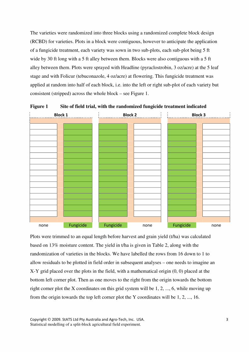
5. Analysis of the data as a split-block or strip-plot experiment
In practice, there were four strata in this experiment. Stratum 1 relates to the formation of
blocks, as has been discussed. Then:
Stratum 2. Plot units within blocks for randomising varieties.
In each block, individual plots are formed to
accommodate the varieties. Technically these are 1/16
block shapes of dimension 5ft by 65 ft – we will call
these plots PlotVar for simplicity. Normally, a 65 ft drill
pass would be planted and the desired plot alley (if
needed) would be cut out with a tiller or mower as
needed to accommodated plot maintenance, application
of treatments, and harvest. In this trial, a 5 ft alley was
left in the middle anticipating the fungicide application,
and allowing farmers an area to walk in the middle of
each block and make comparisons of fungicide
treatments on each variety. This is just an RCBD for
varieties, so to test for varieties, the Block.Variety interaction is used.
2
3
33
3 3
4 4
4
4
44
4
44
4
4
4
4
5
55
5
5
6
Final-stratum residuals
4
6
1
8
3
10
5
12
14
16
4
2
62
1 : -0.4
4 : 0.2
3 : -0.0
2 : -0.2
5 : 0.4
Notice that even with a badly
specified model, the contour plot
appears to detect a trend top to
bottom. The contour ellipses appear
elongated left to right. Again, we will
re-examine this plot later with a more
appropriate set of residuals.
Copyright 2009. StATS Ltd Pty Australia and Agro-Tech, Inc. USA. 17
Statistical modelling of a split-block agricultural field experiment.
Stratum 3. Plot units within blocks for randomising fungicides.
In each block, the fungicide treatment described earlier was applied to the left
or right half at random. Hence for testing the fungicide treatment we use half-
block plots – we will call these plots PlotFung for simplicity. This is just an
RCBD for fungicide, so to test for the fungicide, the Block.Fungicide
interaction is used.
Stratum 4. Plot units within blocks for comparing fungicides across varieties.
Individual plot yields are for one variety with either a fungicide applied or not.
Hence the Variety.Fungicide interaction is tested using a residual based on
individual plots that are 5 ft by 30 ft. This unit is simply the
Block.Variety.Fungicide interaction.
The random model is therefore
Block+Block.PlotVar +Block.PlotFung +Block.PlotVar.PlotFung
which can be simplified to
Block/(PlotVar +PlotFung)
Notice this is not a split-plot design. That design would have the allocation of the fungicide at
random in every variety-plot. The randomizations of the fungicide would not all be to the left
half or the right half of the block.
The ANOVA for this split-block model is as follows.
Source of variation d.f. s.s. m.s. v.r. F pr. Block stratum 2 0.94068 0.47034
Block.PlotVar stratum
Variety 15 9.62752 0.64183 9.07 <.001 Residual 30 2.12226 0.07074 3.31
Block.PlotFung stratum
Fungicide 1 4.84112 4.84112 10.32 0.085 Residual 2 0.93820 0.46910 21.94
Block.PlotVar.PlotFung stratum
Variety.Fungicide 15 0.63413 0.04228 1.98 0.055 Residual 30 0.64141 0.02138 Total 95 19.74531
Copyright 2009. StATS Ltd Pty Australia and Agro-Tech, Inc. USA. 18
Statistical modelling of a split-block agricultural field experiment.
Notice that each F statistic is formed using the Residual from the same stratum. These
residuals are just the interactions described in the discussion above of the four strata. The
stratum variances are estimated to be:
Stratum variance effective d.f. variance component Block 104.349 2.000 -0.329 Block.Variety 15.692 30.000 5.474 Block.Fungicide 103.919 2.000 6.198 Block.Variety.Fungicide 4.744 30.000 4.744
What was a significant block effect when analysed as an RCBD has been eradicated
when analysed as a split-block design.
The previous P value for the Variety.Fungicide interaction (0.767) has collapsed to
0.055, just failing to reach 5% significance. The difference is that the appropriate
denominator MS is now less than half what it was (0.02138 compared to 0.05971)
when an RCB analysis was used, and hence the F statistic is more than double the
previous value (0.71, now 1.98). However, is the statistical evidence in line with our
expectations? If not, are the differences we are trying to detect too small for the
number of replicates used in the experiment? Or is there a problem with our
assumptions? A plot of varietal means suggest there should be a detectable
interaction, with the effect of applying the fungicide greater for some varieties than
for others.
Notice that the residuals now appear in each variety-plot as +value, -value. This follows
from the model: for a balanced split-block design, it can be shown that the residuals sum
to zero over each factor combination. A contour plot of these residuals would therefore be
quite misleading. It would be better to temporarily restrict the plot only to (say) the left
hand set of residuals in each block.
Copyright 2009. StATS Ltd Pty Australia and Agro-Tech, Inc. USA. 19
Statistical modelling of a split-block agricultural field experiment.
To check our assumptions an inspection of the residuals is necessary. Part of the output is a
list of any residual whose standardized value is outside (-2, +2). What is given is the raw
(Final stratum only) residual as well as its standard error:
Block 1 Variety 1989 (Grandin) Fungicide Fungicide 0.182 s.e. 0.082
Hence, once the residuals are saved, the standardized values can be calculated.
Block 1 Block 2 Block 3
16 1.219 -1.219 0.321 -0.321 0.197 -0.197
15 -0.192 0.192 1.154 -1.154 0.774 -0.774
14 -0.767 0.767 0.554 -0.554 -2.776 2.776
13 -0.127 0.127 0.705 -0.705 -0.132 0.132
12 -0.671 0.671 1.034 -1.034 -0.555 0.555
11 0.573 -0.573 0.680 -0.680 -1.732 1.732
10 -0.811 0.811 -1.726 1.726 -0.278 0.278
9 1.006 -1.006 -1.921 1.921 0.539 -0.539
8 1.615 -1.615 -0.240 0.240 0.565 -0.565
7 0.611 -0.611 -0.185 0.185 1.730 -1.730
6 0.042 -0.042 0.241 -0.241 -0.010 0.010
5 1.231 -1.231 0.459 -0.459 0.441 -0.441
4 -0.578 0.578 -0.212 0.212 1.246 -1.246
3 -2.222 2.222 1.150 -1.150 0.465 -0.465
2 -1.161 1.161 -1.112 1.112 -0.626 0.626
1 0.231 -0.231 -0.901 0.901 0.152 -0.152
1.5
1.7
1.9
2.1
2.3
2.5
2.7
2.9
3.1
3.3
18
41
(R
ed
Fif
e)
19
03
(M
arq
uis
)
19
69
(W
ad
ron
)
19
70
(E
ra)
19
79
(Le
n)
19
84
(S
toa
)
19
86
(B
utt
e)
19
88
(A
mid
on
)
19
89
(G
ran
din
)
19
90
(2
37
5)
19
99
(P
ars
ha
ll)
19
99
(R
ee
de
r)
20
00
(A
lse
n)
20
04
(S
tee
le-N
D)
20
05
(G
len
n)
20
06
(H
ow
ard
)
Me
an
yie
ld (
t/h
a)
Plot of means
Fungicide
No Fungicide
Copyright 2009. StATS Ltd Pty Australia and Agro-Tech, Inc. USA. 20
Statistical modelling of a split-block agricultural field experiment.
However, a visual check on the standardised residuals suggests that there are too many runs
of residuals of the same size to be comfortable with their randomness in field position. The
picture is more like one would find with errors which are autoregressive-correlated. There is
a well known data set that can be used to demonstrate this. Temperatures were taken on a
single beaver every 10 minutes. Compare the plot of temperature versus time for this beaver,
and compare that with a plot of random normal data whose mean and standard deviation are
exactly the same as the beaver’s.
The horizontal line is the mean of the beaver’s temperatures. In the top plot, you can see that
the residuals (temperature minus mean temperature) have long runs of the same sign; in the
bottom plot, they are noisily +/- with no apparent long runs of the same sign. For the beaver
temperatures, a time series analysis indicates that the animal’s temperature at any given teime
36.2
36.4
36.6
36.8
37.0
37.2
37.4
37.6
0 20 40 60 80 100 120
Te
mp
era
ture
(°° °°C
)
Sampling occasion
Plot of a beaver's temperature
36.2
36.4
36.6
36.8
37.0
37.2
37.4
37.6
0 20 40 60 80 100 120
Te
mp
era
ture
(°° °°C
)
Sampling occasion
Plot of random temperatures
Copyright 2009. StATS Ltd Pty Australia and Agro-Tech, Inc. USA. 21
Statistical modelling of a split-block agricultural field experiment.
depends in a linear fashion directly on its temperature only at the previous time. This is called
an autoregressive model of order 1, or an AR1 process. Of course the temperature will
depend indirectly on the earlier temperatures as well. There are some applications where the
process at time t depends directly on the two previous times - this is known as an AR2
process. We don’t go beyond AR2 processes when modelling in field trials, as AR1 and AR2
processes generally prove adequate.
6. A row × column analysis of the data
The split-block analysis with random blocks implies several things about the correlation
between plot yields in the field:
Yields from plots in one block are uncorrelated with those from plots in another
block.
Yields from two varieties to which a fungicide has been applied are uniformly
correlated, i.e. they have the same correlation irrespective of whether they come from
plots close together or far apart. This correlation is the same as the uniform
correlation among plots in a block which had no fungicide applied.
Yields from plots in a block that contain the same variety but different strip-plot
treatment (the fungicide) are uniformly correlated, but with a different correlation
than that above.
Yields from different varieties and different fungicide treatments are also uniformly
correlated, again with a different correlation than the two structures above, and again
irrespective of whether they come from plots close together or far apart
These are fairly unreasonable structures for field trials. As mentioned already, plots closer
together are likely to be more highly correlated than plots far apart. Moreover, if two plots at
the end of one block are correlated, and two plots at the start of the next block are also
correlated, it is more likely that the plot at the end of one block is also correlated with that at
the start of the next contiguous block.
Copyright 2009. StATS Ltd Pty Australia and Agro-Tech, Inc. USA. 22
Statistical modelling of a split-block agricultural field experiment.
Consequently, the six row-plots across the field in this trial are likely to be all correlated, with
a correlation structure that declines with distance apart.
Similarly, the sixteen plots in a column down each block are also likely to be correlated, in
general with a different correlation than for the row plots, but also with a correlation structure
that declines with distance apart. We might expect this correlation to be the larger, because
the plots are each only 5 ft wide and share a 30 ft side.
Models that allow this kind of structure are AR1 and AR2 processes for rows and columns.
We generally make an assumption that the two-dimensional correlation structure is
multiplicative. The alternative is that it is unstructured, and this gives rise to a inordinate
number of parameters to estimate.
How is this achieved?
We have already shown how a uniform correlation structure is built into a model: move the
random block effect into the error term, defining the error so that all plots in the field are
indexed (e.g. Block.Plot), then setting a uniform correlation structure among the plots with an
independent structure among the blocks.
In the field plan now under consideration, rather than thinking of the experiment as 3
contiguous blocks, each having 16 contiguous row-plots and two contiguous column-plots,
we think of it as having 16 contiguous row-plots (Y) and 6 contiguous column-plots (X). We
then explore AR1 and AR2 structures for both rows and columns for the random model X.Y,
using change in deviance to detect significantly better structures. Here X and Y need to be
declared factors.
Another variant is to allow for a fixed trend in the rows or columns. Here an examination of
the row-yield averages suggests that no such trend exists. An examination of the column-
yield averages is dangerous since the fungicide treatment is confounded with any detected
trend. Furthermore, the trend detected when the data were analysed as an RCBD indicated the
trend across columns changed within blocks for the two fungicide treatments, which is just a
Block.Fungicide interaction; hence using a split-block analysis, which incorporates this
interaction, should effectively remove this trend.
Since we have detected too many runs of positive and negative residuals in the field when the
yields are analysed as a strip-block design, the possibility of correlated plots in the row (Y)
Copyright 2009. StATS Ltd Pty Australia and Agro-Tech, Inc. USA. 23
Statistical modelling of a split-block agricultural field experiment.
and column (X) directions can now be assessed. We therefore fitted the following models for
X.Y as the random model:
1. AR2 for X and AR2 for Y
2. AR2 for X and AR1 for Y
3. AR1 for X and AR2 for Y
4. AR1 for X and AR1 for Y
5. Id for X and AR1 for Y (Id, shortcut for Identity, represents uncorrelated plots)
6. AR1 for X and Id for Y
The deviances and the changes in deviance as you compare models are given in the following
table. For example, if the deviance for model (2) is not significantly different to that for
model (1), then the more simple model (2) – it has one fewer correlation parameter - is
judged to be adequate. Judgment is based on the change in deviance using a χ2 distribution
with change in degrees of freedom to assess the P value.
X Y deviance d.f.
Change in
deviance
Change
in d.f. P value
AR2 AR2 -102.06 59
AR2 AR1 -101.86 60 0.20 1 0.655
AR2 AR2 -102.06 59 AR1 AR2 -100.39 60 1.67 1 0.196
AR1 AR1 -100.29 61 0.10 1 0.752
id AR1 -81.98 62 18.31 1 <0.001
AR1 AR1 -100.29 61 AR1 id -70.86 62 29.43 1 <0.001
It is clear that the AR2×AR1 model is just as good as the AR2×AR2 model (P = 0.655). We
could have explored the simpler model in the X direction instead: the AR1×AR2 model is
also just as good as the AR2×AR2 model (P = 0.196).
Next, we chose to check whether an AR1×AR1 model is just as adequate as an AR2×AR1
model. Again, the simpler AR1×AR1 model is adequate (P = 0.752).
Copyright 2009. StATS Ltd Pty Australia and Agro-Tech, Inc. USA. 24
Statistical modelling of a split-block agricultural field experiment.
Finally, we found that the id×AR1 model is statistically worse than the AR1×AR1 model
(P < 0.001), as is the AR1×id model (P < 0.001). This means that the yield in any plot
depends directly on the neighbouring plots in both directions. Ticking the Covariance Model
option of LMM allows a visual explanation of the plot structure. The full analysis is given in
the Appendix.
Firstly, the correlation between neighbouring yields from plots immediately above or below
each other is 0.699. The first 10 rows and columns of the correlation matrix for plots
vertically aligned is:
1 1.000
2 0.699 1.000
3 0.489 0.699 1.000
4 0.342 0.489 0.699 1.000
5 0.239 0.342 0.489 0.699 1.000
6 0.167 0.239 0.342 0.489 0.699 1.000
7 0.117 0.167 0.239 0.342 0.489 0.699 1.000
8 0.082 0.117 0.167 0.239 0.342 0.489 0.699 1.000
9 0.057 0.082 0.117 0.167 0.239 0.342 0.489 0.699 1.000
10 0.040 0.057 0.082 0.117 0.167 0.239 0.342 0.489 0.699 1.000
1 2 3 4 5 6 7 8 9 10
The correlation between neighbouring yields from plots immediately to the left or right of
each other is 0.648. There are only six columns in the field, so the 6×6 correlation matrix for
plots horizontally aligned is:
1 1.000
2 0.648 1.000
3 0.420 0.648 1.000
4 0.272 0.420 0.648 1.000
5 0.176 0.272 0.420 0.648 1.000
6 0.114 0.176 0.272 0.420 0.648 1.000
1 2 3 4 5 6
For plots in different rows and columns, simply multiply the correlations from these two
tables for the number of rows and number of columns apart. For example, the two plots
diagonally alongside each other (and hence down one row and across one column) will be
correlated as 0.699×0.648=0.453 under this model.
Using this more sensitive analysis, there is now a strong interaction (P=0.009) between
varieties and fungicide. We are generally interested in comparing the fungicide effect for
each of the varieties. Notice that because plots are correlated, the standard error of a mean
Copyright 2009. StATS Ltd Pty Australia and Agro-Tech, Inc. USA. 25
Statistical modelling of a split-block agricultural field experiment.
difference will change (in this case only slightly) depending on the random allocation of
varieties to plots - i.e. to their distance apart. For this discussion we have extracted the
standard errors of those differences only.
Mean Mean
Difference Variety Fungicide No fungicide s.e.d.
1841 (Red Fife) 2.359 1.987 0.372 0.128
1903 (Marquis) 1.967 1.813 0.154 0.124
1969 (Wadron) 2.734 2.198 0.536 0.125
1970 (Era) 2.841 2.465 0.376 0.128
1979 (Len) 2.356 2.160 0.196 0.120
1984 (Stoa) 3.219 2.504 0.715 0.119
1986 (Butte) 2.785 2.374 0.411 0.121
1988 (Amidon) 2.858 2.551 0.307 0.126
1989 (Grandin) 2.495 2.158 0.337 0.122
1990 (2375) 2.827 2.560 0.267 0.127
1999 (Parshall) 2.897 2.607 0.290 0.129
1999 (Reeder) 3.354 2.752 0.603 0.126
2000 (Alsen) 2.604 2.368 0.237 0.124
2004 (Steele-ND) 2.871 2.529 0.341 0.128
2005 (Glenn) 2.934 2.614 0.320 0.124
2006 (Howard) 3.085 2.593 0.492 0.127
In fact, these means are slightly modified from those from the split-block analysis (as a more
complex spatial model has been fitted). The means from the two analyses are compared in the
following tables and plots.
Variety Fungicide No Fungicide Fungicide No Fungicide
Means from split-block Means from AR1×AR1
1841 (Red Fife) 2.47 1.92 2.36 1.99
1903 (Marquis) 2.06 1.76 1.97 1.81
1969 (Wadron) 2.66 2.06 2.73 2.20
1970 (Era) 3.01 2.54 2.84 2.47
1979 (Len) 2.44 2.12 2.36 2.16
1984 (Stoa) 3.18 2.35 3.22 2.50
1986 (Butte) 2.76 2.31 2.79 2.37
1988 (Amidon) 3.05 2.65 2.86 2.55
1989 (Grandin) 2.46 1.86 2.50 2.16
1990 (2375) 2.97 2.64 2.83 2.56
1999 (Parshall) 3.09 2.84 2.90 2.61
1999 (Reeder) 3.20 2.58 3.35 2.75
Copyright 2009. StATS Ltd Pty Australia and Agro-Tech, Inc. USA. 26
Statistical modelling of a split-block agricultural field experiment.
2000 (Alsen) 2.67 2.46 2.60 2.37
2004 (Steele-ND) 2.96 2.47 2.87 2.53
2005 (Glenn) 3.07 2.82 2.93 2.61
2006 (Howard) 3.16 2.65 3.09 2.59
Variety Fungicide No Fungicide Fungicide No Fungicide
Ranks from split-block Ranks from AR1×AR1
1841 (Red Fife) 13 14 14 15
1903 (Marquis) 16 16 16 16
1969 (Wadron) 12 13 11 12
1970 (Era) 7 7 8 9
1979 (Len) 15 12 15 13
1984 (Stoa) 2 10 2 8
1986 (Butte) 10 11 10 10
1988 (Amidon) 6 4 7 6
1989 (Grandin) 14 15 13 14
1990 (2375) 8 5 9 5
1999 (Parshall) 4 1 5 3
1999 (Reeder) 1 6 1 1
2000 (Alsen) 11 9 12 11
2004 (Steele-ND) 9 8 6 7
2005 (Glenn) 5 2 4 2
2006 (Howard) 3 3 3 4
The effect can be seen for example with Reeder. Under the split-block model, it is ranked 1st
when a fungicide is applied and 6th
when none is applied; under the spatial model it is top
ranked under both fungicide and control. A comparison of means plots from the two analyses
is given on the following page, with the change in rank for Reeder highlighted.
Copyright 2009. StATS Ltd Pty Australia and Agro-Tech, Inc. USA. 27
Statistical modelling of a split-block agricultural field experiment.
1.5
1.7
1.9
2.1
2.3
2.5
2.7
2.9
3.1
3.3
18
41
(R
ed
Fif
e)
19
03
(M
arq
uis
)
19
69
(W
ad
ron
)
19
70
(E
ra)
19
79
(Le
n)
19
84
(S
toa
)
19
86
(B
utt
e)
19
88
(A
mid
on
)
19
89
(G
ran
din
)
19
90
(2
37
5)
19
99
(P
ars
ha
ll)
19
99
(R
ee
de
r)
20
00
(A
lse
n)
20
04
(S
tee
le-N
D)
20
05
(G
len
n)
20
06
(H
ow
ard
)
Me
an
yie
ld (
t/h
a)
Plot of means
Fungicide
No Fungicide
1.5
1.7
1.9
2.1
2.3
2.5
2.7
2.9
3.1
3.3
3.5
18
41
(R
ed
Fif
e)
19
03
(M
arq
uis
)
19
69
(W
ad
ron
)
19
70
(E
ra)
19
79
(Le
n)
19
84
(S
toa
)
19
86
(B
utt
e)
19
88
(A
mid
on
)
19
89
(G
ran
din
)
19
90
(2
37
5)
19
99
(P
ars
ha
ll)
19
99
(R
ee
de
r)
20
00
(A
lse
n)
20
04
(S
tee
le-N
D)
20
05
(G
len
n)
20
06
(H
ow
ard
)
Me
an
yie
ld (
t/h
a)
Plot of means under an AR1××××AR1 spatial model
Fungicide
No Fungicide
Copyright 2009. StATS Ltd Pty Australia and Agro-Tech, Inc. USA. 28
Statistical modelling of a split-block agricultural field experiment.
7. Practical Summary
Statistical
Initial data analysis indicated a significant variety effect and non significant fungicide effect
(P = 0.085) and variety by fungicide interaction (P = 0.055). The lack of significance was
surprising to both agronomist and statistician, as a simple plot of varietal means suggests
there should be a detectable interaction. Residual analysis indicated failure in assumptions
when using a tradition ANOVA approach for analysis. The residuals were not particularly
random which suggested that an alternative model should be fitted. A row × column analysis
was completed and various correlations structures explored. Deviance was used to compare
the models and an AR1 × AR1 correlation structure was chosen as the best fit. The fungicide
effect (P = 0.001) and variety × fungicide interaction (P = 0.009) were significant when a
better statistical model were used. Standard errors were decreased and ranks of varieties
changed. The linear mixed model (REML) approach provided an improved model and
analysis of this field experiment.
Agronomic
The significant variety x fungicide interaction indicates that farmers should not apply
fungicide treatment to every variety of wheat and expect similar yield responses.
Consideration must be made as to what variety is grown and to what the potential yield
response is to fungicide treatment. Certain varieties will provide greater return on investment
than others, and this risk must be considered as actual market price and yield fluctuate. In this
trial, Reeder (1999) and Stoa (1984) had the greatest yield responses and were the top two
yielding varieties when treated with fungicide. Waldron (1969) had the third largest yield
response from fungicide treatment, but only ranked 11th
in grain yield when treated with
fungicide. Red Fife (1841) and Marquis (1803), the oldest varieties and considered by some
the true heritage type wheats in this trial in this experiment, did not respond as well to
fungicide application as Reeder, Stoa or Waldron. Yield response of wheat to fungicides is
very variable. Evaluation of potential yield response must be based on specific variety
information and not generalized based on historical time of development.
Copyright 2009. StATS Ltd Pty Australia and Agro-Tech, Inc. USA. 29
Statistical modelling of a split-block agricultural field experiment.
Appendix 1. REML variance components analysis assuming an
AR1×AR1 spatial model Response variate: Yield Fixed model: Constant + Variety + Fungicide + Variety.Fungicide Random model: X.Y Number of units: 96 X.Y used as residual term with covariance structure as below Sparse algorithm with AI optimisation Covariance structures defined for random model Covariance structures defined within terms: Term Factor Model Order No. rows X.Y X Auto-regressive (+ scalar) 1 6 Y Auto-regressive 1 16 Residual variance model Term Factor Model(order) Parameter Estimate s.e. X.Y Sigma2 0.114 0.0379 X AR(1) phi_1 0.6478 0.0947 Y AR(1) phi_1 0.6992 0.0819 Estimated covariance models Variance of data estimated in form: V(y) = Sigma2.R where: V(y) is variance matrix of data Sigma2 is the residual variance R is the residual covariance matrix Residual term: X.Y Sigma2: 0.1137 R uses direct product construction Factor: X Model: Auto-regressive Covariance matrix: 1 1.000 2 0.648 1.000 3 0.420 0.648 1.000 4 0.272 0.420 0.648 1.000 5 0.176 0.272 0.420 0.648 1.000 6 0.114 0.176 0.272 0.420 0.648 1.000 1 2 3 4 5 6
Copyright 2009. StATS Ltd Pty Australia and Agro-Tech, Inc. USA. 30
Statistical modelling of a split-block agricultural field experiment.
Factor: Y Model: Auto-regressive Covariance matrix (first 10 rows only): 1 1.000 2 0.699 1.000 3 0.489 0.699 1.000 4 0.342 0.489 0.699 1.000 5 0.239 0.342 0.489 0.699 1.000 6 0.167 0.239 0.342 0.489 0.699 1.000 7 0.117 0.167 0.239 0.342 0.489 0.699 1.000 8 0.082 0.117 0.167 0.239 0.342 0.489 0.699 1.000 9 0.057 0.082 0.117 0.167 0.239 0.342 0.489 0.699 1.000 10 0.040 0.057 0.082 0.117 0.167 0.239 0.342 0.489 0.699 1.000 1 2 3 4 5 6 7 8 9 10 Deviance: -2*Log-Likelihood Deviance d.f. -100.29 61 Note: deviance omits constants which depend on fixed model fitted. Tests for fixed effects Sequentially adding terms to fixed model Fixed term Wald statistic n.d.f. F statistic d.d.f. F pr Variety 212.98 15 14.11 44.7 <0.001 Fungicide 20.26 1 20.26 10.3 0.001 Variety.Fungicide 40.64 15 2.71 31.5 0.009