Waves Random Media 10 (2000) 381–394. Printed in the UK PII: S0959-7174(00)12591-1
Statistical moments of travel times at second order in isotropicand anisotropic random media
B Iooss†, Ph Blanc-Benon‡ and C Lhuillier†† CEA Cadarache, DRN/DER/SSAE/LSMN, 13108 St Paul lez Durance, France‡ Laboratoire de Mecanique des Fluides et d’Acoustique, URA CNRS 5509, Ecole Centralede Lyon, BP 163, 69131 Ecully Cedex, France
Abstract. We study the high-frequency propagation of acoustic plane and spherical waves inrandom media. With the geometrical optics and the perturbation approach, we obtain the travel-time mean and travel-time variance at the second order. The main hypotheses are the Gaussiandistribution of the acoustic speed perturbation and a factorized form for its correlation function. Thesecond-order travel-time variance explains the nonlinear behaviour at large propagation distanceobserved with numerical experiments based on ray tracing. Usually, homogeneity and isotropy ofthe refractive index are considered. Using the geometrical anisotropy hypothesis we extend thetheory to a general class of statistically anisotropic random media.
1. Introduction
The theory of wave propagation in turbulent media is founded on the statistical representationof isotropic and homogeneous turbulence (Tatarskii [25]). High-frequency propagation inrandom media has been studied extensively, and there exists a vast amount of literature on thesubject. The basic theory considered a plane wave in an isotropic and homogeneous randommedium (Chernov [5]) or in a locally isotropic and homogeneous random medium (Tatarskii[25]). To make the statistical inference possible, waves have to meet many heterogeneitiesduring their propagation. This condition is expressed by
L� X (1)
where X is the propagation distance and L is the characteristic length of the inhomogeneities.The modern theory of wave propagation in random media uses the parabolic approximation
to connect fluctuations of a plane or spherical wave to medium variations (Rytov et al [20]).The parabolic approximation neglects backscattering by assuming a dominant wavelength λwhich is shorter than the heterogeneities sizes:
λ� L. (2)
On one hand, with an additional Markovian hypothesis, we are able to study statistical momentsof the full wavefield; on the other hand, the Rytov approximation permits one to deal withlog amplitude and arrival time fluctuations. The Rytov approximation is valid provided thewavefield fluctuations are smooth, which means that diffraction effects are small (Rytov et al[20], Shapiro et al [23], Samuelides [21]).
One of the effects of random heterogeneities is the velocity shift effect which states thatthe apparent velocity of the wave is larger than the average velocity of the medium. This isin accordance with Fermat’s principle: the wave path minimizes the travel time of the wave.Theoretically, this can be explained by a second-order derivation of the average travel time(Roth et al [19], Samuelides and Mukerji [22], Samuelides [21]).
Another well known effect is the linear increase of the first-order travel-time variancewith the propagation distance (Chernov [5]). However, nonlinear effects appear at a certainpropagation distance (Karweit et al [13]). This phenomenon is closely related to the occurrenceof first caustics (Kulkarny and White [17], Blanc-Benon et al [1, 2]).
In this paper, we are concerned with the travel time in its natural domain of validity:the geometrical optics theory, which neglects all diffraction phenomena. In the next section,general model and travel-time expressions are given. Therefore, we present the developmentat the second order of the travel-time mean and variance in isotropic media. To validate ourresult on the travel-time variance, we compare theoretical predictions and numerical resultsobtained by the ray tracing and the Gaussian beam summation methods. In the final section, weextend the formulae to a well known class of anisotropic model in geostatistics: the geometricalanisotropy.
2. Travel times in random media
We consider the propagation of monochromatic acoustic waves, which satisfy the Helmholtzequation, in an inhomogeneous motionless medium: u(r, t) = u(r) e−iω0t , where u is thewavefield, r the point location, t the time and ω0 the acoustic frequency. In the high-frequencyregime, the wavefield u(r) in a random medium is a random function with fluctuations of itstravel time T (r) and amplitude A(r): u(r) = A(r) eiω0 T (r).
A rigorous consideration of the travel times requires the geometrical optics approximation.In the geometrical optics, diffraction phenomena are ignored because the size of the first Fresnelzone is much smaller than the transverse scale length of heterogeneities l⊥:
√λX � l⊥. (3)
Therefore, the travel time satisfies the eikonal equation [∇T (r)]2 = 1c2(r)
, where c is the
acoustic speed. Moreover, we suppose that 1c2(r)
deviates only weakly from a constant valueand we write
[∇T (r)]2 = 1
c2(r)= 1
c20
[1 + ε(r)] (4)
where c0 is a constant acoustic speed and ε are small fluctuations (|ε| � 1).We expand T as a power series in the small perturbation parameter ε. Keeping terms
up to the second order gives T (r) = T0 + T1(r) + T2(r). Let r = (r‖, r⊥) be a vector inthe propagation basis ((r‖, 0) is oriented along the propagation direction) and let X be thepropagation distance (see figure 1). For a spherical wave, the different terms contributing tothe travel time are expressed as
T0(r) = ‖r‖c0= Xc0
(5)
T1(r) = 1
2c0
∫r
ε(r′) dr′ = 1
2c0
∫ X
0ε(r ′, r⊥) dr ′ (6)
T2(r) = − 1
4c0
∫ X
0
[∫ r ′
0
r ′′
r ′∇⊥ε(r ′′, r⊥) dr ′′
]2
dr ′. (7)
Statistical moments of travel times at second order 383
Figure 1. Geometry of the problem, graphical illustration of the anisotropy: the horizontal a,vertical b, parallel l‖ and transverse l⊥ correlation lengths.
For a plane wave, expressions are similar except for T2 where r ′′r ′ = 1.
T0 is the deterministic term corresponding to a constant speed medium, which leads to astraight ray. T1 gives the first-order fluctuations by integrating medium perturbations alongthe straight ray. T2 describes the leading-order effect of the ray bending due to perturbations(Snieder and Aldridge [24]). It has been given for spherical waves by Boyse and Keller [3].
When ray bending increases, stronger nonlinear travel-time perturbations appear, andhigher-order terms must be taken into account (Snieder and Aldridge [24]).
3. The isotropic case
3.1. The random models
Let us suppose that ε(r) is a weak and centred random field: |ε| � 1, 〈ε〉 = 0. If c(r) is theacoustic speed, we obtain by linearization of equation (4):
c(r) = c0[1− 1
2ε(r)]
(8)
where c0 is the average acoustic speed (〈c〉 = c0). To make statistical inference possible,we suppose that ε is statistically homogeneous. Therefore, ε is defined by its autocorrelationfunction (or covariance) Cε(r) = 〈ε(r + r1)ε(r1)〉, where r and r1 are two point locations.
With the additional hypothesis of isotropy, the correlations of ε are independent by rotation,then Cε(r) = Cε(‖r‖). We define a new function, called the standardized covariance N :
Cε(r) = Cε(x, y, z) = σ 2ε N
(‖r‖L
)(9)
which has a standard deviation and a correlation length normalized to unity. Finally, a fewstatistical parameters describe ε: its standard deviation σε =
√〈ε2(r)〉, its correlation length
L which is a typical size of the heterogeneities, and its standardized covariance N .
384 B Iooss et al
To calculate statistical moments of T2, we will use two parameters which depend on thecovariance structure N :
A1 =∫ ∞
0N(u) du A2 =
∫ ∞0
N ′(u)u
du (10)
where N ′ is the derivative of N . Let us evaluate the coefficients A1 and A2 for differentcovariance functions.
• The Gaussian covarianceN(h) = exp(−h2) leads to media with very smooth fluctuations,with only one scale of inhomogeneity: the correlation length. In this case, we haveA1 = 1
2
√π and A2 = −√π .
• The exponential covarianceN(h) = exp(−h)models rough models, with a slow decreaseof the correlations (as a function of h). For this model, A1 = 1 and A2 is undefined: ourapproach will be not valid.• The spectral density�(k) of a random medium is the Fourier transform of its covariance.
The power spectrum �(k) ∝ (1 + k2L2)−p−3/2 (p ∈ [0, 1]) is a generalization ofthe Kolmogorov spectrum (�(k) ∝ k−11/3). The Kolmogorov spectrum models theenergy cascade in a turbulent fluid (Tatarskii [25]) between the external range L (energyproduction scale) and the inertial range l0 (dissipation scale). Therefore, this spectrum isdefined for
2π
L� k � 2π
l0
and the power spectrum for k � 2πl0
.The power spectrum leads to a covariance of the form
N(h) = 21−p
�(p)hpKp(h)
whereKp is the modified Bessel function of second type and of order p. This model gives
A1 =√π�( 1
2 + p)
�(p)
and
A2 =√π [(−1 + 2p)�(− 1
2 + p) + 2�( 12 + p)]
4�(p).
Therefore, A2 is defined for p > 12 . The case p = 1
2 corresponds to the exponentialcovariance.• The modified Von Karman model is derived from the power model by taking p = 1
3 .To take into account the small inhomogeneities, it introduces in the spectrum a Gaussianfilter exp(−k2/k2
m) where km = 5.92l0
is a cut-off frequency. The modified Von Karmancovariance is written as
C(h) = 1.685C2nk−2/3m
[1F1
(− 13 ; 3
2 ;− 14k
2mh
2)]
where Cn is a constant and (1F1) is the confluent hypergeometric function. Therefore, wetake
N(h) = 1F1(− 1
3 ; 32 ;− 1
4k2mh
2)
and we obtain, A1 = 2.583km
and A2 = 1.076km
.
Statistical moments of travel times at second order 385
3.2. Travel-time mean and variance
We denote by T P and T S the travel times of a plane and of a spherical wave. At first order, thetravel time mean is zero because 〈ε〉 = 0 (see equation (6)). The average travel time at secondorder is deduced from equation (7) and the derivation is given in appendix A. We obtain
〈T (r)〉 = T0(r) + 〈T2(r)〉 (11)
〈T P2 (r)〉 = 3〈T S2 (r)〉 =A2
8
σ 2ε
c0
X2
L. (12)
For the variance, Var(T ) = Var(T1 +T2) = 〈(T1 +T2)2〉−〈T1 +T2〉2 = Var(T1)+Var(T2)+
〈T1T2〉. The travel-time variance at first order Var(T1) is a well known result called the Chernovprediction (Chernov [5], Keller [14]). With the hypothesis of a Gaussian distribution for ε,〈T1T2〉 = 0 because this term contains the third-order moment of ε which is zero in theGaussian case. The derivation of the travel-time variance at second order Var(T2) is made inappendix B. We obtain
Var[T (r)] = Var[T1(r)] + Var[T2(r)] (13)
Var[T P1 (r)] = Var[T S1 (r)] =A1
2
σ 2ε
c20
LX = A1
2
σ 2ε
c20
L2X
L(14)
Var[T P2 (r)] = 9 Var[T S2 (r)] =A2
2
32
σ 4ε
c20
X4
L2= A
22
32
σ 4ε
c20
L2
(X
L
)4
. (15)
Therefore, neglecting Var(T2) with respect to Var(T1) leads to the explicit condition
X � ALσ−2/3ε
A = 2
(2A1
A22
)1/3
(plane wave)
A = 2
(18A1
A22
)1/3
(spherical waves).
(16)
For a Gaussian covariance, A � 1.653 for a plane wave and A � 3.438 for a spherical one.Note that relation (16) provides an estimate of the validity of the asymptotic series in terms ofthe distance of propagation X with respect to L and σε .
3.3. Connection with the probability density of the occurrence of caustics
As an example let us consider an isotropic random medium characterized by a Gaussiancovariance. In figure 2, we compared the second-order travel-time variances of plane wavesVar[T P2 (r)], and of spherical waves Var[T S2 (r)] both with the first-order Chernov estimates.The travel-time variances are plotted in terms of the normalized distance X/L. Thesecomparisons are done for σε = 0.01 and two values of the correlation length L: L = 1and 0.5 m. We clearly observed that the departures from the Chernov prediction increase withtravel distance. The conditions (16) become X
L� 35 for the plane wave case, and X
L� 74 for
the spherical wave case. We observe visually that the nonlinearity effects due to the second-order term Var(T2) appear at a shorter distance and increase much faster in the plane wavecase than in the spherical wave case. Indeed, caustics appear at shorter distances for planewaves than for spherical waves (Kulkarny and White [17]). The effect of travel distance hasbeen observed previously by Juve et al [11] for transmission of acoustic waves through two-dimensional (2D) isotropic turbulence and by Karweit et al [13] for three-dimensional (3D)random velocity fields. The reason for this behaviour seems to be directly linked to the existence
386 B Iooss et al
Figure 2. Theoretical travel-time variances versus normalized distanceX/L. Curves are plotted fora Gaussian covariance with two scales L(1 m; 0.5 m), a velocity c0 = 1500 m s−1 and σε = 0.01.
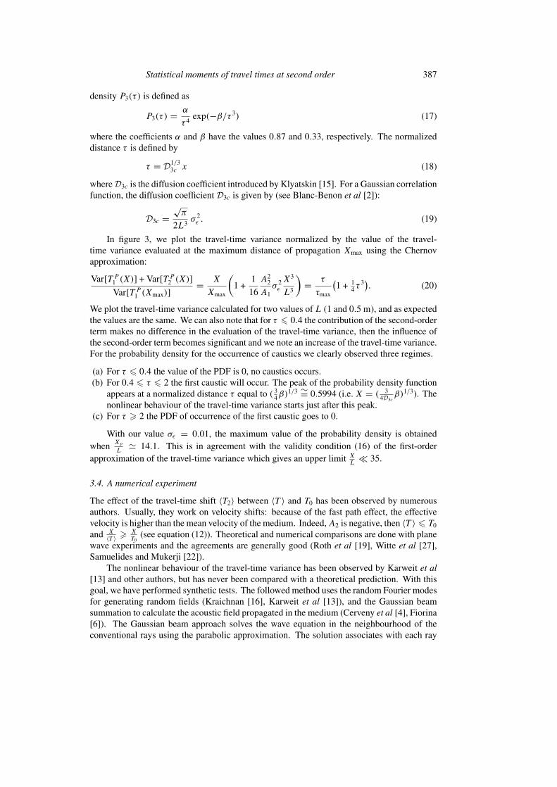
Figure 3. Illustration of the connection between the occurrence of the first caustic and thenonlinear evolution of the travel-time variance. Curves are plotted in the case of a plane wave(c0 = 1500 m s−1, ε has a Gaussian covariance, σε = 0.01, L = 1 and 0.5 m).
of caustics. To consolidate this point of view, we plot in figure 3 the probability density of theoccurrence of the first caustics as a function of a normalized distance of propagation τ .
For an initially plane wave propagating through 3D isotropic turbulence the probability
Statistical moments of travel times at second order 387
density P3(τ ) is defined as
P3(τ ) = α
τ 4exp(−β/τ 3) (17)
where the coefficients α and β have the values 0.87 and 0.33, respectively. The normalizeddistance τ is defined by
τ = D1/33c x (18)
whereD3c is the diffusion coefficient introduced by Klyatskin [15]. For a Gaussian correlationfunction, the diffusion coefficient D3c is given by (see Blanc-Benon et al [2]):
D3c =√π
2L3σ 2ε . (19)
In figure 3, we plot the travel-time variance normalized by the value of the travel-time variance evaluated at the maximum distance of propagation Xmax using the Chernovapproximation:
Var[T P1 (X)] + Var[T P2 (X)]
Var[T P1 (Xmax)]= X
Xmax
(1 +
1
16
A22
A1σ 2ε
X3
L3
)= τ
τmax
(1 + 1
4τ3). (20)
We plot the travel-time variance calculated for two values of L (1 and 0.5 m), and as expectedthe values are the same. We can also note that for τ � 0.4 the contribution of the second-orderterm makes no difference in the evaluation of the travel-time variance, then the influence ofthe second-order term becomes significant and we note an increase of the travel-time variance.For the probability density for the occurrence of caustics we clearly observed three regimes.
(a) For τ � 0.4 the value of the PDF is 0, no caustics occurs.(b) For 0.4 � τ � 2 the first caustic will occur. The peak of the probability density function
appears at a normalized distance τ equal to ( 34β)
1/3 ∼= 0.5994 (i.e. X = ( 34D3cβ)1/3). The
nonlinear behaviour of the travel-time variance starts just after this peak.(c) For τ � 2 the PDF of occurrence of the first caustic goes to 0.
With our value σε = 0.01, the maximum value of the probability density is obtainedwhen Xp
L� 14.1. This is in agreement with the validity condition (16) of the first-order
approximation of the travel-time variance which gives an upper limit XL� 35.
3.4. A numerical experiment
The effect of the travel-time shift 〈T2〉 between 〈T 〉 and T0 has been observed by numerousauthors. Usually, they work on velocity shifts: because of the fast path effect, the effectivevelocity is higher than the mean velocity of the medium. Indeed,A2 is negative, then 〈T 〉 � T0
and X〈T 〉 �
XT0
(see equation (12)). Theoretical and numerical comparisons are done with planewave experiments and the agreements are generally good (Roth et al [19], Witte et al [27],Samuelides and Mukerji [22]).
The nonlinear behaviour of the travel-time variance has been observed by Karweit et al[13] and other authors, but has never been compared with a theoretical prediction. With thisgoal, we have performed synthetic tests. The followed method uses the random Fourier modesfor generating random fields (Kraichnan [16], Karweit et al [13]), and the Gaussian beamsummation to calculate the acoustic field propagated in the medium (Cerveny et al [4], Fiorina[6]). The Gaussian beam approach solves the wave equation in the neighbourhood of theconventional rays using the parabolic approximation. The solution associates with each ray
388 B Iooss et al
Figure 4. Comparison between theoretical and numerically computed travel-time variances (ins2).
a beam having a Gaussian amplitude normal to the ray. The solution for a given source isthen constructed by a superposition of Gaussian beams along nearby rays. The rays are givenfrom the standard ray-tracing technique, but the use of Gaussian beams has the advantage ofavoiding eigenray computations to find the travel times at fixed receivers.
The acoustic velocity has an isotropic Gaussian covariance withL = 0.1 m, σε = 0.0038,c0 = 1509.13 m s−1, and we perform 400 different realizations. The medium has a width of4 m and a height of 1 m. In each realization, we consider a spherical wave. The source islocated at (0; 0.5), the global propagation direction is horizontal, and 201 rays are regularlylaunched in an opening angle of 10◦. 20 receivers are regularly placed on the horizontal axiseach 0.2 m spacing, with 0.2 m � X � 4 m where X is the propagation distance.
In figure 4, we compare numerical results with theoretical curves: the Chernov solution
Var(T1) =√π
4
σ 2ε
c20
LX
and the new solution
Var(T1) + Var(T2) =√π
4
σ 2ε
c20
LX +π
288
σ 4ε
c20
X4
L2.
We observe that the nonlinear behaviour is correctly predicted by the new solution.
4. Extension to geometrically anisotropic media
The isotropy hypothesis breaks down in a lot of concerned media, e.g. in the middle atmospherefor radiophysical studies (Rytov et al [20]), in the ocean (Flatte et al [7]), in 3D turbulent flows(Karweit and Blanc-Benon [12]), in sedimentary basins for the seismic exploration problem
Statistical moments of travel times at second order 389
Figure 5. Example of a statistically anisotropic velocity field (axis in metres). The velocity hasa Gaussian covariance, with c0 = 1509 m s−1, 〈c2〉 = 16 (m s−1)2, θ = 11.5◦, a = 1 m,b = 0.25 m.
(Iooss [9, 10], Samuelides and Mukerji [22]), in the lithosphere and asthenosphere for theseismological framework (Flatte and Wu [8]), etc.
In a 3D anisotropic random medium, instead of having a single correlation length a(which is a measure of the typical heterogeneity size), three correlation lengths a, b and care needed. Therefore, the refractive index covariance C(x, y, z) cannot be reduced to C(r)with r =
√x2 + y2 + z2 as in the isotropic case. To simplify the problem, we work with a 2D
geometry throughout this section. The extension to 3D is given in appendix C.
4.1. The geometrical anisotropy hypothesis
We assume that ε is stationary at second order, with an anisotropic covariance Cε(x, y) ofgeometrical type (Wackernagel [26]):
Cε(x, y) = σ 2ε N
[√(x cos θ + y sin θ)2
a2+(x sin θ − y cos θ)2
b2
](21)
where σ 2ε is the variance of the fluctuations, N the standardized covariance (the statistical
structure), θ the stratification angle (with the horizontal axis), a the correlation length in the θdirection and b the correlation length in the normal direction of θ . We admit that the correlationlengths are measures of the heterogeneity scales.
In real problems, taking into account such an anisotropy is important; e.g. the seismicheterogeneities are often strongly stratified and gently sloping; in the atmosphere or in theocean, the wind or current direction can lead to inadequacy between the propagation directionand the anisotropy axis; in industrial problems (such as pipe flows of a fluid), particulargeometries provoke inclined heterogeneities stratification. A random medium with inclinedstratification is shown in figure 5.
For wavefield propagation in such media, the correlation lengths of interest are thoseparallel (l‖) and transverse (l⊥) to the propagation direction (see figure 1). We consider r
390 B Iooss et al
oriented along the principal propagation direction, which forms an angle α with the horizontalaxis. Then r = (r cosα, r sin α) and we can write
Cε(r) = σ 2ε N
[√r2
a2(cosα cos θ + sin α sin θ)2 +
r2
b2(cosα sin θ − sin α cos θ)2
]. (22)
In the propagation direction Cε(r) = σ 2ε N(
rl‖), and we deduce the parallel correlation length
l‖. In the orthogonal direction, Cε(−r sin α, r cosα) = σ 2ε N(
rl⊥), and we find the transverse
correlation length l⊥. We obtain
1
l2‖= (cosα cos θ + sin α sin θ)2
a2+(cosα sin θ − sin α cos θ)2
b2
1
l2⊥= (− sin α cos θ + cosα sin θ)2
a2+(sin α sin θ + cosα cos θ)2
b2.
(23)
In the example of figure 5 (a = 1, b = 0.25, θ = 11.5◦), if we study a horizontal wave (α = 0),we obtain l‖ � 0.792 and l⊥ � 0.255.
Finally, on the basis of the wave propagation direction, we have
Cε(r) = Cε(r‖, r⊥) = σ 2ε N
√√√√ r2‖l2‖
+r2⊥l2⊥
. (24)
If α = θ = 0 and a = b, we return to the isotropic model with l‖ = l⊥ = a = b andCε(r) = σ 2
ε N(ra) where r = ‖r‖.
4.2. Statistical moments of travel times
As in the isotropic case, we start from equations (6) and (7). The main difference in thetheoretical derivations is for formula (9). From (24), we obtain
∇2⊥Cε(X, r⊥)|r⊥=0 = σ
2ε
X
l‖l2⊥N ′(X
l‖
). (25)
Therefore, the same techniques than in appendices A and B lead to
〈T P1 (r)〉 = 〈T S1 (r)〉 = 0 (26)
〈T P2 (r)〉 = 3〈T S2 (r)〉 =A2
8
σ 2ε
c0
l‖l2⊥X2 (27)
Var[T P1 (r)] = Var[T S1 (r)] =A1
2
σ 2ε
c20
l‖X (28)
Var[T P2 (r)] = 9 Var[T S2 (r)] =A2
2
32
σ 4ε
c20
l2‖l4⊥X4. (29)
Neglecting Var(T2) leads to an explicit condition involving X, l‖, l⊥ and σε :
X � A
(l4⊥l‖
)1/3
σ−2/3ε (30)
where A is defined as in the isotropic case by equation (16).
Statistical moments of travel times at second order 391
5. Conclusion
The new result of this paper is the calculation of the second-order term of the travel-timevariance in random media. After a linear increase (first order or Chernov approximation), thetravel-time variance explodes at a certain propagation distance due to the occurrence of the firstcaustics. This behaviour has been qualitatively and quantitatively validated with a numericalexperiment based on ray tracing and the Gaussian beam summation method.
This theory is valid at second order, for applications in which the travel-time perturbation isonly weakly nonlinear. Moreover, our results are valid in the geometrical optics approximation,when diffraction effects are negligible. The scattering phenomenon, which occurs at a certainpropagation distance (see equation (3)), modifies the behaviour of the travel-time variance(Rytov et al [20]).
In this work, we have used a general form of the medium covariance which permits one toextract the standardized covariance, i.e. the canonical form of the covariance. This formulationmakes the consideration of statistically anisotropic random media easier, and we have given ageneral formula for the mean and variance of the travel times. The same method would allowus to obtain expressions for the travel-time covariance (Iooss [10]) and the statistical momentsof the amplitude.
Appendix A. Travel-time mean at second order
We calculate 〈T2〉 in the geometrical optics for a 3D plane wave, with the same approach asBoyse and Keller [3]. We have (see equation (7))
T2(r) = − 1
4c0
∫ X
0
[∫ r ′
0∇⊥ε(r ′′, r⊥) dr ′′
]2
dr ′. (A1)
Taking the average value, we obtain
〈T2(r)〉 = − 1
4c0
∫ X
0
∫ r ′
0
∫ r ′
0〈∇⊥ε(r ′′1 , r⊥)∇⊥ε(r ′′2 , r⊥)〉 dr ′′1 dr ′′2 dr ′
= 1
4c0
∫ X
0
∫ r ′
0
∫ r ′
0∇2⊥Cε(r
′′1 − r ′′2 , r⊥)|r⊥=0 dr ′′1 dr ′′2 dr ′ (A2)
because Cε′(r) = −C ′′ε (r) (Papoulis [18]).By using (9), we have
∇2⊥Cε(X, r⊥)|r⊥=0 = σ 2
ε
LXN ′(X
L
). (A3)
With the new variables r ′′ = r ′′1 − r ′′2 and s = 12 (r′′1 + r ′′2 ), equations (A2) and (A3) lead to
〈T2(r)〉 = σ 2ε
4c0L
∫ X
0
∫ r ′
0
∫ ∞0
N ′(r ′′/L)r ′′
dr ′′ ds dr ′. (A4)
We have extended the integration domain of r ′′ to infinity becauseN ′(r ′′/L)/r ′′ is concentratedin the |r ′′| < L domain, and we have assumed X � L (equation (1)).
Finally, with a last variable change, we obtain from (A4)
〈T2(r)〉 = σ 2ε
8c0
X2
L
∫ ∞0
N ′(r ′)r ′
dr ′. (A5)
392 B Iooss et al
For a spherical wave (see equation (7)), we have to add r ′′1r ′r ′′2r ′ in the integrand of
equation (A2). We obtain
〈T2(r)〉 = σ 2ε
4c0L
∫ X
0
∫ r ′
0
∫ r ′
0
(s2
r ′2− r ′′2
4r ′2
)N ′(r ′′/L)r ′′
dr ′′ ds dr ′. (A6)
As N ′(r ′′/L)/r ′′ is concentrated in the |r ′′| < L domain, the term with r ′′24r ′2 has a negligible
contribution to the integration. Keeping the other term, we finally obtain
〈T2(r)〉 = 1
3
σ 2ε
8c0
X2
L
∫ ∞0
N ′(r ′)r ′
dr ′. (A7)
The travel-time variance of a spherical wave is one third of that of a plane wave.
Appendix B. Travel-time variance at second order
We calculate Var(T2) = 〈T 22 〉 − 〈T2〉2 in the geometrical optics for a plane wave. From (A1),
×ϒε(r ′1 − r ′′1 , r ′2 − r ′′2 , 0) + ϒε(r′1 − r ′2, r ′′1 − r ′′2 , 0) + ϒε(r
′1 − r ′′2 , r ′2 − r ′′1 , 0).
(B4)
We simplify the three terms in the same manner as in appendix A. For example, for the firstterm, the variable changes are h1 = r ′1−r ′′1 , h′1 = 1
2 (r′1 +r ′′1 ), h2 = r ′2−r ′′2 , and h′2 = 1
2 (r′2 +r ′′2 ).
By extending the integration domain of h′1 and h′2 to infinity, the three terms lead to the sameresult. Hence, we have
〈T 22 〉 =
3X4
64c20
σ 4ε
L2
∫ ∞0
∫ ∞0
N ′(h1/L)N′(h2/L)
h1h2dh1 dh2. (B5)
Statistical moments of travel times at second order 393
Finally, we have calculated the travel-time variance at second order of a plane wave:
Var(T2) = X4
32c20
σ 4ε
L2
[∫ ∞0
N ′(u)u
du
]2
du. (B6)
By the same arguments as in appendix A, the travel-time variance of a spherical wave is 19 of
that of a plane wave.
Appendix C. Geometrical anisotropy in 3D
For three-dimensional random media, expressions are more complex than in 2D. Let (l1, l2, l3)be the correlation lengths in a (e1, e2, e3) orthogonal basis, and the matrix
Λ =(
1
l21,
1
l22,
1
l23
)I3
with I3 the 3D identity matrix. The (e1, e2, e3) basis is defined by a 3D rotation of the(Ox,Oy,Oz) = (h1, h2, h3) initial Cartesian basis, which involves three elementary rotationsof angles θ1, θ2, θ3 (see Wackernagel [26]). The rotation matrix Q is written as
Q =
cos θ3 sin θ3 0
− sin θ3 cos θ3 0
0 0 1
1 0 0
cos θ2 sin θ2 0
− sin θ2 cos θ2 0
cos θ1 sin θ1 0
− sin θ1 cos θ1 0
0 0 1
.
(C1)
The propagation direction of the wave is defined by the azimuthal angle α1 in the (e1, e2)
basis, and the polar angle α2 (with e3). Therefore, we call the propagation vector d‖ and thetransverse vectors d⊥1 and d⊥2. We choose the orthogonal basis (d‖,d⊥1,d⊥2) with d⊥1 inthe vertical plane (including e3) which forms an angle α1 with e1:
d‖ =
cosα1 sin α2
sin α1 sin α2
cosα2
d⊥1 =
− cosα1 cosα2
− sin α1 cosα2
sin α2
d⊥2 =
sin α1
− cosα1
0
(C2)
Let h be a vector, we define the standardized covariance N by
Cε(h) = σ 2ε N(√hTQTΛQh
). (C3)
Therefore, to find the correlation length in the wave propagation basis, let us replace h by hd‖,hd⊥1 and hd⊥2. For example, if h is oriented along the propagation direction,
Cε(h) = σ 2ε N
(h
l‖
)= σ 2
ε N(h
√dT‖QTΛQd‖
).
We find
1
l2‖= dT‖QTΛQd‖
1
l2⊥1
= dT⊥1QTΛQd⊥1
1
l2⊥2
= dT⊥2QTΛQd⊥2. (C4)
An important particular case of 3D anisotropic media is the transverse isotropic model:l⊥1 = l⊥2 = l⊥. In the general case of a geometrical anisotropy, the formulae (27)–(30) remainvalid by replacing 1
l2⊥with 1
l2⊥1+ 1l2⊥2
[10].
394 B Iooss et al
References
[1] Blanc-Benon P, Juve D and Comte-Bellot G 1991 Occurence of caustics for high-frequency waves propagatingthrough turbulent fields Theor. Comput. Fluid Dynam. 2 271–8
[2] Blanc-Benon P, Juve D, Ostashev V E and Wandelt R 1995 On the appearance of caustics for plane sound-wavepropagation in moving random media Waves Random Media 5 183–99
[3] Boyse W and Keller J B 1995 Short acoustic, electromagnetic and elastic waves in random media J. Opt. Soc.Am. 12 380–9
[4] Cerveny V, Popov M M and Psencik I 1982 Computation of wave fields in inhomogeneous media—Gaussianbeam approach Geophys. J. R. Astron. Soc. 70 109–28
[5] Chernov L A 1960 Wave Propagation in a Random Medium (New York: McGraw-Hill)[6] Fiorina D 1998 Application de la methode de sommation de faisceaux Gaussiens a l’etude de la propagation
ultrasonore en milieu turbulent These Ecole Centrale de Lyon[7] Flatte S M, Dashen R, Munk W H, Watson K M and Zachariasen F 1979 Sound Transmission throug a Fluctuating
Ocean (New York: Cambridge University Press)[8] Flatte S M and Wu R S 1988 Small-scale structure in the lithosphere and asthenosphere deduced from arrival
time and amplitude fluctuations at NORSAR J. Geophys. Res. 93 6601–14[9] Iooss B 1998 Seismic reflection traveltimes in two-dimensional statistically anisotropic random media Geophys.
J. Int. 135 999–1010[10] Iooss B 1998 Tomographie statistique en sismique reflexion: estimation d’un modele de vitesse stochastique
These Ecole des Mines de Paris[11] Juve D, Blanc-Benon P and Hugon-Jeannin Y 1991 Simulation numerique de la propagation en milieu aleatoire
Publ. LMA 125 245–55[12] Karweit M and Blanc-Benon P 1993 Arrival-time variance for acoustic propagation in 3-D random media: the
effect of lateral scale C. R. Acad. Sci., Paris II 316 1695–702[13] Karweit M, Blanc-Benon P, Juve D and Comte-Bellot G 1991 Simulation of the propagation of an acoustic wave
through a turbulent velocity field: a study of phase variance J. Acoust. Soc. Am. 89 52–62[14] Keller J B 1962 Wave propagation in random media Symp. Applied Math. vol 16 (Providence, RI: American
Mathematical Society) pp 227–46[15] Klyatskin V I 1993 Caustics in random media Waves Random Media 3 93–100[16] Kraichnan R H 1970 Diffusion by a random velocity field Phys. Fluids 13 22–31[17] Kulkarny V A and White B S 1982 Focusing of waves in turbulent inhomogeneous media Phys. Fluids 25
1770–84[18] Papoulis A 1965 Probability, Random Variables and Stochastic Processes (New York: McGraw-Hill)[19] Roth M, Muller G and Snieder R 1993 Velocity shift in random media Geophys. J. Int. 115 552–63[20] Rytov S M, Kravstov Y A and Tatarskii V I 1987 Principles of Statistical Radiophysics (Berlin: Springer)[21] Samuelides Y 1998 Velocity shift using the Rytov approximation J. Acoust. Soc. Am. 104 2596–603[22] Samuelides Y and Mukerji T 1998 Velocity shift in heterogeneous media with anisotropic spatial correlation
Geophys. J. Int. 134 778–86[23] Shapiro S, Schwarz R and Gold N 1996 The effect of random isotropic inhomogeneities on the phase velocity
of seismic waves Geophys. J. Int. 127 783–94[24] Snieder R and Aldridge D F 1995 Perturbation theory for travel times J. Acoust. Soc. Am. 98 1565–9[25] Tatarskii V I 1961 Wave Propagation in a Turbulent Medium (New York: Dover)[26] Wackernagel H 1995 Multivariate Geostatistics (Berlin: Springer)[27] Witte O, Roth M and Muller G 1996 Ray tracing in random media Geophys. J. Int. 124 159–69