Statistical precipitation downscaling in central Sweden

with the analogue method

Fredrik Wetterhall*, Sven Halldin, Chong-yu Xu

Air and Water Science, Department of Earth Sciences, Uppsala University, Villavagen 16, SE-752 36 Uppsala, Sweden

Received 9 December 2003; revised 3 September 2004; accepted 10 September 2004

Abstract

Most climate predictions show significant consequences globally and regionally, but many of its critical impacts will occur at

sub-regional and local scales. Downscaling methods are, thus, needed to assess effects of large-scale atmospheric circulation on

local parameters such as precipitation and runoff. This study aims at evaluating the analogue method (AM) as a benchmark

method for precipitation downscaling in northern Europe. The predictors used in this study were daily and monthly gridded sea-

level pressures from 1960 to 1997 in an area 45–758N and 308W–408E with a resolution of 5!58 long-lat. Analogues for daily

and monthly precipitation at seven precipitation stations in south-central Sweden were established with two techniques,

principal-component analysis (PCA) and the Teweles-Wobus score (TWS). The results showed that AM downscaling on both

daily and monthly basis was commonly generally much better than a random baseline but depended on the objective function

used for assessment; PCA and TWS produced similar results in most cases but TWS was superior in simulating precipitation

duration and intensity. Downscaling was improved when seasonality was included and when the SLP field was confined to those

geographical areas that contributed most to precipitation in south-central Sweden.

q 2004 Elsevier B.V. All rights reserved.

Keywords: Analogue method; Downscaling; Precipitation; PCA; Teweles-Wobus score; Sweden

1. Introduction

The interaction between large-scale circulation and

local weather is a growing field of research, since

global-climate studies with General Circulation

Models (GCM) show significant consequences glob-

ally and regionally, but many of its critical impacts

will occur at sub-regional and local scales, i.e. at

0022-1694/$ - see front matter q 2004 Elsevier B.V. All rights reserved.

doi:10.1016/j.jhydrol.2004.09.008

* Corresponding author. Tel.: C46 18 471 22 59; fax: C46 18 55

11 24.

E-mail address: fredrik.wetterhall@hyd.uu.se (F. Wetterhall).

drainage basins and agricultural areas (Wilby and

Wigley, 1997). There can be great variability on the

local scale, and GCMs have trouble simulating

precipitation and river runoff correctly (Xu, 1999).

Downscaling methods to assess the effect of large-

scale circulations on local parameters have, thus,

received much attention during the last decade (Wilby

and Wigley, 1997).

Statistical downscaling methods establish a stat-

istical relationship between one or several large-scale

meteorological variables, commonly atmospheric

circulation, and local-scale variables. This is done

Journal of Hydrology 306 (2005) 174–190

www.elsevier.com/locate/jhydrol

F. Wetterhall et al. / Journal of Hydrology 306 (2005) 174–190 175

by translating anomalies of the large-scale flow

(predictors) into anomalies of some local climate

variable (predictand; Zorita and von Storch, 1999).

Also temperature (Brandsma and Buishand, 1997) and

humidity (Beckmann and Buishand, 2002) have been

used as predictors in downscaling studies. In principle

any kind of variable can be used as predictor as long

as it is reasonable to expect that there exists a

relationship between the predictor and the predictand.

Compared to dynamic downscaling, statistical down-

scaling has the advantages of being computationally

cheap and easily adjusted to new areas. Statistical

downscaling also requires very few parameters and

this makes it attractive for many hydrological

applications (Wilby et al., 2000). A statistical down-

scaling scheme can use GCM output as predictor data

to model predictands in a perturbed climate if it can be

assumed that the derived relationships are valid in a

future climate (Zorita et al., 1995). It is obvious that

the validity of the result is first of all dependent on the

GCM’s ability to model the predictor. A disadvantage

of statistical downscaling is that it requires long

and homogenous data series for establishment and

validation of the statistical relationship (Heyen et al.,

1996).

The analogue method (AM) is a simple statistical

method based on finding an analogue to a target

climate variable from an earlier observation in a

similar weather situation. It was first used to assess

weather predictability and for short-term forecasts

(Lorenz, 1969; Martin, 1972) and has later been used

in downscaling studies. The AM can be carried out in

different ways depending on the technique to establish

the analogue. Principal-component analysis (PCA) of

the predictor field is the most common technique

(Zorita et al., 1995; Cubasch et al., 1996) but

other techniques include the Teweles-Wobus score

(TWS) (Obled et al., 2002) and nearest-neighbour

resampling technique (Brandsma and Buishand, 1998,

Buishand and Brandsma, 2001). AM gives the

downscaled data the same statistical properties as

the training data. Since it assumes a static relationship

between predictor and predictand, it cannot, in the

version used here, be used to downscale climate

scenarios unless the perturbed future climate shows

the same variability as the present. AM is still useful

as a benchmark method for evaluation of more

sophisticated methods (Zorita and von Storch, 1999).

It can also be used to evaluate statistical properties of

the predictor and its relationship to the predictand

(Bardossy and Caspary, 1990; Zorita et al., 1995;

Widmann and Schar, 1997).

Precipitation is the most important driving variable

in most hydrological modelling and analysis. Precipi-

tation is governed by complicated, inherently non-

linear and extremely sensitive physical processes

(Bardossy and Plate, 1991) and this makes a

deterministic downscaling model practically imposs-

ible. Precipitation simulation is, thus, commonly done

with statistical methods both in time and space (e.g.

Cowpertwait et al., 1996a,b; Busuioc et al., 2001).

The two main objectives of this study were (1) to

evaluate AM as a benchmark method for future

statistical downscaling of precipitation in the Baltic-

Sea basin, and (2) to use AM to investigate the

statistical properties of the large-scale sea-level

pressure (SLP) field and precipitation in central

Sweden. Specific goals to meet the first objective

were (1) to compare the PCA and TWS techniques to

establish precipitation analogues, and (2) to evaluate

combinations of objective functions and evaluation

variables to find the most suitable ones for a given

application. Specific goals to meet the second

objective were (1) to find the geographical regions

whose SLP fields govern the precipitation in central

Sweden, and (2) to establish seasonality patterns in

the relationship between large-scale atmospheric

circulation and precipitation for the study region.

The analyses were carried out on daily and monthly

timescales in order to investigate the capability of AM

to model extreme events as well as precipitation

totals.

2. Data

2.1. Predictands

The predictand or the variable to be downscaled

was daily and monthly precipitation. Daily data from

1960 to 2000 were purchased from the Swedish

Meteorological and Hydrological Institute (SMHI) for

ten stations situated around Uppsala in south-central

Sweden (Fig. 1). The stations were selected within the

southern NOPEX region (Halldin et al., 1999),

approximately at 608N latitude and 188W longitude,

Fig. 1. Selected predictor grid area in the study. The location of the seven precipitation stations in the NOPEX region are marked with

black dots.

F. Wetterhall et al. / Journal of Hydrology 306 (2005) 174–190176

in order to support other climate-related research

carried out for this region. We retained 37 years

(1 January 1960 to 31 December 1997) of data from

seven stations (Table 1) for which the data sets were

reasonably complete. 3.9% of the data were missing

for the period 1961–1990, whereas the time series

were 100% complete for the period 1991–1997. The

37-year period was broken up into a training period

and a validation period based on the completeness

of the data. The training period was taken as

1961–1990 and the validation period as the remaining

7 years 1991–1997. Since precipitation occurrence

Table 1

Precipitation stations in south-central Sweden

No. Station Latitude Lon

1 Vasteras-Hasslo 59835 051 00 168

2 Sundby 59841 046 00 168

3 Skultuna 59842 050 00 168

4 Sala 59854 016 00 168

5 Uppsala flygplats 59853 043 00 178

6 Dralinge 59859 032 00 178

7 Vattholma 5981 044 00 178

a Meter above sea level.b Averaged over the period 1961–1990.

and amounts are stochastic by nature, gap-filling

would not improve results so we did not pre-process

data in any way. The data we received were original

measurements. SMHI also supplied correction factors

to account for wind loss, adhesion to, and evaporation

from measurement vessels at each station (Eriksson,

1983). We used the corrected data in this study.

2.2. Predictors

The selection of appropriate predictor, or charac-

teristics from the large-scale atmospheric circulation,

gitude Altitude

(masl)a

Mean annual

precipitation (mm)b

37 057 00 15 583

39 038 00 35 684

26 010 00 40 680

39 038 00 60 666

35 036 00 21 653

34 025 00 30 635

43 027 00 25 682

F. Wetterhall et al. / Journal of Hydrology 306 (2005) 174–190 177

is one of the most important steps in a downscaling

exercise. Three main factors constrain the choice of

predictors, i.e. data should be (1) reliably simulated by

GCMs, (2) readily available from archives of GCM

output, and (3) strongly correlated with the surface

variables of interest (Wilby et al., 1999). The

predictor used in this study was the daily sea-level

pressure (SLP) continuing from 1899 to present. The

data comes from several sources and is available for

free on the NCEP/NCAR internet site http://dss.ucar.

edu/pub/reanalysis/. The monthly dataset was down-

loaded from the same site, and consists of the time

series corrected by Trenberth and Paolino (1980). The

geographical extent, 45–758N, 308W–408E was cho-

sen to include all areas with noticeable influence on

the circulation patterns that govern weather in

Scandinavia (Hanssen-Bauer and Førland, 2000).

The dataset is gridded with a resolution of 5!58

long-lat and data are given twice daily, at 00:00 and

12:00 UTC. Only the data for 12:00 UTC were

retained because of missing data during the period

1961–1997. Still 1.2% of the data were missing, but it

was assumed that this would not cause significant

problems in our analysis.

3. The analogue downscaling method

The analogue method (AM) uses, in a straightfor-

ward way, an historical record of predictor and

predictand to simulate the future of the predictand.

The basic idea is to find a predictor from the historical

(also called training) record which has the same

characteristics as a predictor at a given target time

t(day, week, month, etc.). The predictand, S, for the

targeted time t, is simulated by selecting the

predictand at the time u, for which the characteristics

of the predictor F(u) most closely resemble those of

the target F(t). The predictor for this time is called the

analogue to F(t). The analogue is found numerically

by selecting

minjjFðuÞKFðtÞjj (1)

from the training record (Cubasch et al., 1996). The

simulated predictand, S(t), is then assumed equal to

the predictand of the analogue, S(u). In our case this

means that a certain amount of precipitation

(predictand) is attached to a specific pattern of the

large-scale sea-level pressure (SLP) field (predictor).

The target pattern, F(t), can either be observed or

simulated by a GCM. The corresponding target

precipitation estimation SðtÞ is then:

SðtÞ Z SðuÞ (2)

Different techniques exist to numerically select a

minimum value between a target SLP field and its

historical analogue. In this study we evaluate two

techniques. The first is a principal-component anal-

ysis (PCA) of the SLP-anomaly field A. The second is

a pattern-comparison technique that minimises the

pressure gradients of the SLP field.

AM demands long time series for the training data

in order to simulate all kind of events (only events that

have occurred in the historical record can be attributed

as analogues). Two or three decades of data are

normally considered sufficient if the purpose is to

model precipitation.

3.1. The PCA technique

The principal-component analysis (PCA) finds the

underlying properties of the large-scale field by

dividing the anomalies into a number of variability

patterns, all orthogonal to each other (the technique

is also known as empirical orthogonal functions in

meteorological literature). In this case, the field,

A(k,t), is the time (t) series of SLP anomalies at each

5!58 grid point (k) in the selected region (Fig. 1). The

anomaly is defined as the deviation at each grid point

from the average pressure for the training period

1961–1990.

The procedure compares the p eigenvectors, C,

with the largest eigenvalues, l, of the covariance

matrix R of A. The dimensionality of the problem is

then greatly reduced (Zorita et al., 1995):

RC Z Cl (3)

where CZc1; c2;/; cp are the p eigenvectors (or

principal components, PC) of R, and l denotes the

eigenvalues of R.

The anomaly field can be written as:

Aðk; tÞ ZXp

jZ1

bjðtÞcjðkÞC3ðk; tÞ (4)

F. Wetterhall et al. / Journal of Hydrology 306 (2005) 174–190178

where bj(t) is the projection of the anomaly field onto

the pth principal component, cp, and 3(t) is the

variability not described by the p leading principal

components. BðtÞZb1ðtÞ; b2ðtÞ;/; bpðtÞ are also called

expansion coefficients of the equivalent principal

components and are uncorrelated in time, just as the

principal components are uncorrelated in space.

A selection method is then devised. Consider an

atmospheric anomaly pattern which has expansion

coefficients ZZz1; z2;/; zp in the same PC field as

B(t). The analogue of Z is the B(t) that minimises:

Xp

iZ1

ðzi KbiðtÞÞ2 (5a)

Zorita et al. (1995) extend the PCA technique by

introducing weights (di):

Xp

iZ1

½diðzi KbiðtÞÞ2� (5b)

The weights are used to find the proportion of the

PC patterns that has the largest influence on the target

precipitation.

3.2. Teweles-Wobus score

The Teweles-Wobus Score (TWS) compares the

shape of the SLP field, P(k,t), by considering its

gradients instead of its anomalies at each grid point.

TWS was originally developed to evaluate the quality

of geopotential-height forecasts (Teweles and Wobus,

1954). The method uses pressure gradients in N–S and

E–W directions and the analogue is the field (from

time u) that minimises:

TWSðtÞ Z

PIkZi gðk; tÞC

PJkZj gðk; tÞ

PIkZi Gðk; tÞC

PJkZj Gðk; tÞ

(6)

gðk; tÞ Z jðPðk K1; uÞKPðk C1; uÞÞK ðPðk K1; tÞ

KPðk C1; tÞÞj ð7Þ

Gðk; tÞ Z max½jPðk K1; uÞKPðk C1; uÞj;

Pðk K1; tÞKPðk C1; tÞ� ð8Þ

where g(k,t) is the difference in pressure gradient

at grid point k between the analogue (at time u)

and the observed SLP field (at time t). Summation of

gradients in N–S direction is denoted by i and in E–W

direction by j. G(k,t) is the larger gradient of the two.

The gradients were not calculated for the outermost

grid points because surrounding grid points are

required. The gradient field, thus, had 20% less data

than the anomaly field used in the PCA technique.

Both techniques were realized in MATLAB, which

had an efficient PCA routine whereas the TWS was

carried out crudely by looping through all times and

gradient grid points. This made the numerical

efficiency of TWS significantly lower than that of

PCA. Since the TWS technique was developed for

geopotential heights it can only be applied as an

AM with certainty when pressure fields or geopoten-

tial heights are used as predictors, whereas any

predictor and combination of predictors can be used

with PCA.

4. Method evaluation

AM is simple, straightforward and ‘objective’ in

the sense that it contains few fudge factors that can be

manipulated or calibrated. There are still subjective

decisions that must be made to get a good simulation.

A baseline must also be defined against which the

different simulations can be evaluated.

The first subjective decisions depend on the

downscaling goal: is, e.g. precipitation used to predict

floods and inundations or is the closure of the water

balance important? The second set of choices is

somewhat less subjective and depends on the size and

quality of the dataset on which the analysis is made.

They respond to questions such as: how large

geographical area of SLP data is needed to downscale

precipitation? Should seasonality be taken into

account? Different tests were designed to respond to

these two types of questions.

4.1. Objective functions

The choice of objective functions is governed by

the purpose of the study (Obled et al., 2002). If, e.g.

the purpose is to evaluate extreme events, evaluation

parameters that capture those characteristics are

selected. The precipitation to be evaluated is also

time-dependent, so the objective function must be

sensitive to temporal properties.

Table 2

Summary of objective functions and evaluation variables

Objective

function

Evaluation variable Time step

Day Month

Efficiency Precipitation amount x x

RPS Precipitation distribution x x

Dry-spell length distribution x

Residual

(difference

between

downscaled

and

Observed

values)

Average yearly precipitation x x

Maximum precipitation x x

Median precipitation x

Probability of dry following dry x

Probability of wet following wet x

Probability of a wet day x

Length of wet spell x

Length of dry spell x

Average wet day amount x

Standard deviation of wet day

amount

x

F. Wetterhall et al. / Journal of Hydrology 306 (2005) 174–190 179

The first objective function used in the study is

efficiency that is defined as the squared difference

between observed and simulated results divided by

the observed variance.

E Z1

N

1

T

XN

nZ1

XT

tZ1

½sobsðn; tÞKssimðn; tÞ�2

s2n

(9)

where sobs is the observed and ssim is the simulated

precipitation at station n at time t. N is the number of

stations, T is the number of simulated days/months

and s2n is the observed variance of the predictand at

station n (Zorita and von Storch, 1999). A good fit is a

low value on efficiency. The value of E is independent

of the number of stations and the length of the

evaluation period.

The second objective function used in the study is

called The Ranked-Probability Score (RPS), which

evaluates a dimensionless cumulative probability

distribution, in this case of precipitation or duration

of dry spells (Epstein, 1969; Murphy, 1971). Obled et

al. (2002) used this function in a precipitation-

downscaling study. This evaluation criterion is

expressed in Eqs. (10) and (11).

RPS Z1000

N

XN

nZ1

XM

iZ1

½Sn;i K Sn;i�2 (10)

Sn;i ZXi

mZ1

xmðnÞ; Sn;i ZXi

mZ1

xmðnÞ (11)

where M is a predetermined number of classes, xm is

the fraction of days belonging to class m at station n, S

are the probability scores for the observed precipi-

tation and S for the downscaled precipitation. The

probability scores are always calculated for the whole

validation period. The factor 1000 in Eq. (10) is used

to scale the RPS values to a range that is easier to

handle. A value close to 0 denotes a good simulation.

RPS has the property to give probability distributions

of similar structure a lower value compared to the

probability score (PS), which compares individual

probabilities without regard to the structure. RPS has

a subjective component, i.e. how you choose number

of classes and the limits of each class. When used for

precipitation amount, eight classes were chosen

for the daily precipitation: 0 (no rain), 0–1, 1–3,

3–5, 5–10, 10–20, 20–50, and more than 50 mm rain

per day and seven classes for the monthly precipi-

tation: 0–20, 20–35, 35–50, 50–70, 70–100, 100–150

and more than 150 mm per month. When used for

dry-spell length the classes were 7–9, 10–12, 13–15,

16–20, O20 days. The same classes were used for all

stations.

Residuals (i.e. the difference between downscaled

and observed values) were used in this study, in

addition to efficiency and RPS, to evaluate the skills of

the techniques in simulating various precipitation

characteristics such as maximum precipitation, prob-

abilities of a wet or a dry day, lengths of wet and dry

spells, etc. Most of these objective functions were

only used for daily series. The average yearly

precipitation and maximum precipitation for the

whole period were used for both daily and monthly

series. All objective functions (Table 2) were

evaluated for the validation period 1990–1997.

4.2. Spatial coverage and seasonality

The choice of different areas for the predictor field

can influence both results and calculation time. The

spatial correlation of precipitation amounts between

the seven measurement stations were preserved with

the analogue method since the stations were modelled

as a group and not individually. The time scale may

also be an important factor when selecting the area

of influence of the SLP field (Brinkmann, 2002).

The most significant circulation characteristics in time

F. Wetterhall et al. / Journal of Hydrology 306 (2005) 174–190180

and space depend on whether the downscaling is done

on monthly or daily precipitation. A number of tests

were performed to evaluate these conditions.

The relative importance of the grid points in the

SLP field was first investigated. Monthly and daily

simulations were performed where grid points were

successively excluded one by one. The different

objective functions were evaluated graphically as

function of grid points:

GPðiÞ ZXK

kZ1

DðkÞ; k Z 1; 2;/;K; k si (12)

where GP(i) is the grid-point-evaluation function for

grid point i and D is the objective function, and K total

number of grid points. The grid-point-evaluation

maps were then taken as a starting point to find

those areas that contained the most significant SLP

information. The analysis was carried out in analogy

with Obled et al. (2002) but whereas they only varied

window size, we tested spatial windows with different

forms, centres and sizes. The selection of these

windows was subjective but based on areas in the

grid-point-evaluation maps with maxima in GP

values.

Seasonality effects were evaluated by introducing

time windows. The best analogue to a simulated

precipitation could be found for a totally different

season if all training data were used. To avoid this,

training data were restricted to a time window, such

that the analogue had to be selected from the same

time of year as the simulated one. For example, if the

day to simulate was 7 January and the time window 21

days, then the analogue could be selected between 29

December and 17 January any year of the training

period. A 3-month window for the monthly simu-

lations meant that analogues for, e.g. July could be

retrieved from June–August data.

4.3. Calibration and downscaling procedure

We had one possibility to calibrate AM in this

study. By generalising the PCA technique according

to Zorita et al. 1995 (Eq. (5b)) the relative

contributions of each PC could be weighted to

optimise the simulated precipitation. Calibration was

done with brute force by evaluating all objective

functions with a combination of weight values

ranging from 0 to 2.6 in steps of 0.2. Both daily

and monthly calibrations were limited to the first three

PCs since further components added insignificantly to

the result.

The final results were achieved after an iterative

3-step procedure. This procedure was carried out

individually for both techniques (PCA, TWS) and

both time steps (day, month). Step 1 identified the best

spatial window for the SLP field, step 2 identified the

optimal time window, and step 3 calibrated the

weights in Eq. (5b). Since the purpose of this study

was to evaluate AM in a general way, we investigated

steps 1–2 with all objective functions and selected,

subjectively, those simulations that gave good results

for as many functions as possible. The weights in step

3 were, thus, deduced to produce good results in

general. A downscaling application aimed towards a

specific goal could have resulted in other spatial/

seasonal windows and calibration weights.

4.4. Baseline simulations

Randomised daily and monthly simulations were

the baseline comparisons for the two AM techniques.

Each simulation consisted in randomly selecting, for

each day/month of the simulated 1991–1997 period,

an analogue from the training dataset 1961–1990.

Each such random simulation was evaluated with all

of the objective functions. The values of these

functions were averaged from 1000 random

simulations.

5. Results

5.1. Main circulation modes and geographical

areas of influence

The four leading PCs for the daily PCA simulations

explained 83% of the total variance of the SLP-

anomaly field, distributed as 32, 19, 18, and 8% over

PC1–PC4. The monthly analysis was even better with

the four leading PCs explaining 93% of the variation

(Fig. 2a–d). PC1 describes an anticyclonic or cyclonic

circulation in the North Sea (Fig. 2a). This is the most

significant characteristic of the anomaly field and

answers for 32% of the variation. PC2 (Fig. 2b)

represents anomalies in the zonal winds and PC3

Fig. 2. (a–d) The first four principal components (PCs) of the monthly average SLP-anomaly field within the study area. The PCs have been

normalized.

F. Wetterhall et al. / Journal of Hydrology 306 (2005) 174–190 181

(Fig. 2c) anomalies in the meridional winds, explain-

ing, respectively, 21 and 14% of the variation. PC4

represents a more complicated wind field and explain

8% of the variation (Fig. 2d).

The grid-point-evaluation function showed differ-

ent patterns depending on the choice of technique,

time step and objective function. The patterns

generally demonstrated two important areas, one

around the target area in Sweden and one slightly

south of Iceland (Fig. 3e and f). Some patterns

(especially those generated with PCA) also showed an

arctic influence whereas some simulations did not

show any clear pattern at all.

Areal windows based on the previous patterns gave

different results depending on the SLP-field-recog-

nition technique. The TWS technique required larger

spatial windows than the PCA technique and daily

simulations required larger windows than monthly

(Fig. 3a–d). Monthly TWS simulations were signifi-

cantly better with two spatial windows included.

The monthly PCA optimisation was best with only

a small area above the target stations. The area size

influenced the PCA results. The smaller the area, the

more influence from the first principal components.

With a sufficiently small area, the problem reduced to

a mere influence of a high or low pressure given by the

first two PCs. The best PCA simulations were

achieved with the spatial windows in Fig. 3 combined

with weights dZ(1.4 2.0 2.4) for the daily and

dZ(1.1 1.6 0) for the monthly time steps.

5.2. Seasonality

The temporal analysis for the daily time step gave

similar results for the two techniques (based on areal

windows and weights above). The PCA analysis gave

an optimum time window of 15 days, whereas the

TWS window was 19 days. The monthly analysis, on

the other hand gave a significant difference between

PCA and TWS, with windows of 3 months and 1

month, respectively. Different objective functions

responded very differently to time windows of varying

size, as exemplified in Fig. 4. Selecting the optimum

Fig. 4. Dependence of two objective functions on the time-window

size for the TWS technique with daily data. The residuals are

normalized by dividing with each series maximum value.

Fig. 3. Top and centre: optimum area windows for downscaling with daily data using (a) the PCA and (b) the TWS techniques, and for monthly

data using (c) the PCA and (d) the TWS techniques. Bottom: examples of grid-point-evaluation values for monthly downscaling based on (e) the

efficiency with the PCA technique, and (f) RPS of precipitation distribution with the TWS technique. Brighter colors distinguish areas with high

influence on the result whereas darker colors distinguish less influential areas.

F. Wetterhall et al. / Journal of Hydrology 306 (2005) 174–190182

time window was, therefore, subjective and depend-

ing on the aim of the study.

5.3. The capability of AM to downscale precipitation

Simulated daily precipitations show a limited

similarity with observed values for both techniques

even after smoothing with a 5-day-moving-average

filter (Fig. 5). Statistical properties are well captured

and, except the total amounts, significantly better than

the random baseline simulations (Table 3). The TWS

technique underestimates the wet-day amounts

whereas the opposite holds true for PCA.

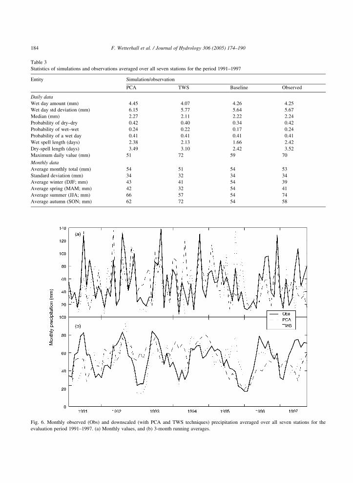
Whereas it is difficult to simulate a daily

precipitation series for a given station with AM, the

temporal variation of monthly values, averaged over

all seven stations, are reasonably well captured by

Fig. 5. Daily precipitation for Vasteras-Hasslo precipitation station during the later part of 1991, observed (Obs) and downscaled with PCA and

TWS techniques (top three diagrammes). The bottom diagram shows the same data smoothed with a 5-day running-average filter.

F. Wetterhall et al. / Journal of Hydrology 306 (2005) 174–190 183

the method (Fig. 6). The average yearly variation is

well simulated (Fig. 7a), although amounts are

underestimated in August and overestimated in

October. The method has difficulties to capture the

annual averages (Fig. 7b). The validation period also

has somewhat lower annual averages than the training

period. Statistical properties are significantly better

simulated with both PCA and TWS than with the

random baseline for all properties except for total

precipitation (Table 3, Fig. 8). The TWS performs

somewhat better than PCA in terms of efficiency and

RPS whereas PCA seems to capture seasonal

precipitation somewhat better than TWS for all

seasons. Both techniques capture the length of dry

spells much better than the baseline simulation

(Fig. 9), whereas TWS seems clearly superior in

capturing duration and intensity of extreme precipi-

tation (Fig. 10).

The iterative three-step procedure for the down-

scaling was evaluated in terms of relative improve-

ment compared to an original simulation where the

whole SLP field was used, no seasonality was taken

into account, and no PCA calibration was performed

(Table 4). Daily simulations show a greater sensitivity

for properties such as dry and wet spells and transition

probabilities, than they do for the general objective

functions efficiency and RPS. Efficiency improve-

ments in monthly simulations are significant for each

step of the PCA technique, whereas results from TWS

are not conclusive. The opposite situation was present

Fig. 6. Monthly observed (Obs) and downscaled (with PCA and TWS techniques) precipitation averaged over all seven stations for the

evaluation period 1991–1997. (a) Monthly values, and (b) 3-month running averages.

Table 3

Statistics of simulations and observations averaged over all seven stations for the period 1991–1997

Entity Simulation/observation

PCA TWS Baseline Observed

Daily data

Wet day amount (mm) 4.45 4.07 4.26 4.25

Wet day std deviation (mm) 6.15 5.77 5.64 5.67

Median (mm) 2.27 2.11 2.22 2.24

Probability of dry–dry 0.42 0.40 0.34 0.42

Probability of wet–wet 0.24 0.22 0.17 0.24

Probability of a wet day 0.41 0.41 0.41 0.41

Wet spell length (days) 2.38 2.13 1.66 2.42

Dry-spell length (days) 3.49 3.10 2.42 3.52

Maximum daily value (mm) 51 72 59 70

Monthly data

Average monthly total (mm) 54 51 54 53

Standard deviation (mm) 34 32 34 34

Average winter (DJF; mm) 43 41 54 39

Average spring (MAM; mm) 42 32 54 41

Average summer (JJA; mm) 66 57 54 74

Average autumn (SON; mm) 62 72 54 58

F. Wetterhall et al. / Journal of Hydrology 306 (2005) 174–190184

Fig. 7. Observed (Obs) and downscaled (with PCA and TWS techniques) (a) 1991–1997 monthly precipitation amounts averaged over all

stations. Observed precipitation is given as box plots giving median, upper and lower quartiles and max and min values. Annual total

precipitation amounts (b) for the validation period 1991–1997. The thick and dotted straight lines denote mean values and standard deviations

for the training period 1961–1990.

F. Wetterhall et al. / Journal of Hydrology 306 (2005) 174–190 185

for the RPS of the monthly downscaling, with the

most noticeable improvement with the TWS

technique.

6. Discussion

The analogue method is a downscaling but not a

modelling method. AM basically reshuffles measured

time-series data so the statistical properties of the

underlying data can be expected to be preserved as

long as the downscaling and training periods have the

same climate. Only weather situations that have

occurred in the past can be simulated with the AM

method, but if the historical dataset contains enough

weather situations the method can be used in

combination with output from climate models to

downscale future weather situations, but this is not

recommended when downscaling singular analogues

to create time series (Buishand and Brandsma, 2001).

More complicated downscaling schemes, such as

regression techniques or weather patterns, also depend

on historical datasets for calibration but can be

assumed to downscale future scenarios better than

AM since these methods have a dynamical relation-

ship between predictor and predictand. This is the

reason for expecting AM to work primarily as a

benchmark for downscaling methods with predictive

capacity. One should on the other hand always be

extremely careful when extrapolating models outside

their calibrated time period.

The ability to capture statistical properties rather

than day to day precipitation (Figs. 9 and 10; Table 3)

is in accordance with other studies, e.g. Zorita and von

Storch (1999) and indicates that the training period

in this study was large enough to incorporate sufficient

precipitation variability. Precipitation is an inherently

stochastic, strongly intermittent, and nonlinear

Fig. 8. The objective functions RPS for precipitation distribution (a and c) and efficiency (b and d) for daily (a and b) and monthly (c and d)

simulations.

F. Wetterhall et al. / Journal of Hydrology 306 (2005) 174–190186

process (Deidda, 1999) that can have great impact on

local climate and water balance (floods and droughts)

over short time periods. Amounts and timing can,

therefore, only be expected to be downscaled with a

sufficient accuracy when averaged over long time

periods. The success of a downscaling method must

instead be evaluated against its capacity to reproduce

statistical properties such as extreme events, transition

probabilities and lengths of dry and wet spells,

distribution of daily and monthly precipitation, and

seasonality. AM is also good as a benchmark method

because of its low degree of subjectivity. AM has no

calibration parameters except for the weights in the

PCA technique. The only other subjective choices

are the geographical extent of the pressure field

(Obled et al., 2002) and size of a time window.

The success of a given method can be fully

evaluated only if the goal is clearly stated. Several

goals, in the form of different objective functions were

used in this study since the purpose was to carry out a

general assessment of AM in northern Europe. If there

is a need to conciliate several, possibly contradictory

goals, this study could be carried further with

multidimensional scaling and correlation analysis.

The presented downscaling results are typical

examples that provided good results for several

objective functions. Table 4 demonstrates that good

results for one objective function are often counter-

balanced by poor results for another. It would, e.g.

have been possible to get better results for the annual

total precipitation (Fig. 7b) but this would have

caused deteriorated distribution properties. A strict

evaluation of the PCA method with adjustable

weights should also have required an independent

evaluation period. The relative merits of the TWS and

PCA techniques are, thus, only given in general terms.

It is clear that one technique may outperform the other

for a specific goal.

The areal window of the predictor is objectively

chosen as the best field concerning the evaluation

parameters. The selected field should be physically

reasonable as a predictor for precipitation in central

Sweden. It is difficult to draw any consistent

conclusion from the areal windows. The results are

the optimum windows for the overall simulation,

and are selected objectively. One might argue that

Fig. 9. Distribution of dry spells. (a) Dry spells longer than 7 days and (b) RPS for the dry-spell distribution.

Fig. 10. Precipitation intensity and duration for all seven

precipitation stations for the whole 1990–1997 evaluation period.

F. Wetterhall et al. / Journal of Hydrology 306 (2005) 174–190 187

the selected windows for the PCA method are too

small to incorporate important processes in the

predictor, and that a larger window is necessary.

The argument against this is that a subjective choice

is then introduced. The optimum area windows for

the PCA methods are small but still physically

reasonable. The areal window with the PCA

technique is centred above the study area and the

anomalies in the MSLP field are thereby dominated

by high or low pressures. If the validation period was

divided into separate seasons the optimal areal

window might look differently.

Johansson and Chen (2003) conducted a study on

the influence of wind and topography in Sweden and

found that the orography is the most important

parameter in mountainous regions, but since the

stations in this study are located in the lowland

areas in Sweden, wind direction is more important

than orography when downscaling precipitation. The

areal window with the TWS technique is larger

meaning that a larger area of influence, than with

the PCA method, is needed to capture the large-scale

wind direction. The split window in the monthly

simulations indicates an area south of Iceland is

important for precipitation, and may be an indicator

Table 4

Improvements in % in the steps of the AM downscaling for a daily and a monthly simulations aiming at good results for as many objective

functions as possible

Entity Simulation technique/procedure

PCA TWS

Area Time Weights Area Time

Daily simulations

Efficiency 8 10 K5 0 K14

RPS, precipitation distribution K5 K40 K16 0 3

Probability wet–wet 7 23 90 0 23

Length of wet spell 8 30 92 0 16

Probability dry–dry 22 64 98 0 K12

Length of dry spell 15 45 95 0 K25

Monthly simulations

Efficiency 27 21 23 10 20

RPS, precipitation distribution 0 K69 7 55 71

Percentages give improvements from the original simulations with (1, area) optimised geographical coverage of the SLP field, (2, time) account

for seasonality, and (3, weights) calibration.

F. Wetterhall et al. / Journal of Hydrology 306 (2005) 174–190188

that westerly winds are important for precipitation in

the study region.

The choice of predictors can also influence the areal

distribution. Obled et al. (2002) used the TWS method

to downscale precipitation in southern France with

pressure fields at different geopotential heights (1000

and 700 hPa) and with different sizes and orientation.

The result was that 700 hPa was the better single

predictor, but the optimum was a combination of fields

at different heights and with a time lag of 12 h. A

similar investigation in this study may have given

similar results, but this was not conducted since the

purpose was to compare two methods, and introducing

more predictors would greatly increase the dimension-

ality and the results would be more difficult to evaluate.

Both the PCA and TWS techniques normally

provided significantly better downscaling results

than the random-downscaling baseline (Table 3,

Figs. 8–10) in all but some foreseeable cases. Both

techniques performed badly, as expected, when it

came to amount and timing of precipitation on

individual days (Fig. 5). It is possible that this result

could be improved if the predictor contained not only

SLP but also humidity of the air mass, i.e. information

on the precipitable water. The inter-annual variations

were not well captured by any of the techniques

(Fig. 7b), but this is a well-known problem (Wilby,

1994; Bardossy et al., 1995; Stehlik and Bardossy,

2002). Both techniques produced, as expected,

average-wet-day amounts and standard deviations

similar to the random baseline downscaling (Table 3).

In most other respects, they performed significantly

better than the baseline, random simulation. The

monthly simulations gave better seasonality than the

baseline (Figs. 6 and 7) for both techniques with a

small advantage of PCA over TWS. Both daily and

monthly simulations gave a clear advantage for both

techniques over the baseline in terms of precipitation–

distribution RPS. We could not find a simple

explanation for the odd behaviour of station six

(Dralinge) when daily simulations were evaluated

with precipitation-distribution RPS (Fig. 8a).

A separate investigation might reveal if this station

has a non-representative precipitation climate, if data

from it contain errors, or if its surroundings were less

than ideal. The monthly simulation efficiency was

higher for both techniques whereas the daily simu-

lation efficiency was, again as expected, only margin-

ally better than that of the baseline (Fig. 8). The PCA

technique is, by far, the most commonly used of the

two. This study shows modest differences in down-

scaling capability between the PCA and TWS

techniques. The PCA technique tended to give slightly

better results than TWS in terms of efficiency.

Efficiency is, however, not an ideal measure for a

discrete variable such as precipitation. It was included

in this study merely because of its widespread use.

When residuals or RPS (i.e. when statistical

F. Wetterhall et al. / Journal of Hydrology 306 (2005) 174–190 189

precipitation properties are important) were important

the TWS often gave similar or better results than

PCA. The TWS technique outperformed PCA in

the downscaling of extreme precipitation events

(Fig. 10). The conceptual simplicity of TWS and its

lower degree of subjectivity could be taken as other

arguments to favour TWS over PCA in future AM

downscaling studies. To improve the numerical

efficiency of TWS it could be motivated to do the

programming in, e.g. FORTAN instead of MATLAB.

The intra-annual variations between observed and

simulated precipitation were smaller during winter

and spring periods than during summer and autumn

(Fig. 7a). The only month where the results were

outside the observed standard deviation limits was

October. The monthly simulations captured much of

the seasonal variations, but precipitation was under-

estimated during the summer and overestimated

during the fall (Table 3). The PCA technique seemed

to capture seasonality slightly better than TWS. It is

possible that the problem with downscaling of inter-

annual precipitation may depend on this seasonality

problem. Simulations improved for the target season

but were poorer for the other seasons when the

evaluation period was chosen as a particular season

instead of the whole period. This suggests that there

could be different optimum temporal and areal

resolutions for different seasons; not surprising since

north-European precipitation is governed by different

processes during different seasons and weather

situations (Stehlik and Bardossy, 2002; Huth and

Kysely, 2000; Wilby, 1994). Another important

aspect is that there might be spatial offsets in the

correlation patterns between predictors and predic-

tands (Wilby and Wigley, 2000). This means that the

most effective target season should not be an entire

year. Another reason to limit the time window is that

certain key evaluation parameters have different

impact at different seasons. Dry spells in Sweden,

e.g. are more common in winter but have the largest

societal impact in summer.

7. Conclusions

This study demonstrated that the analogue method

is well suited as a benchmark method to evaluate

more sophisticated precipitation-downscaling

methods over northern Europe. Previous AM studies

have primarily used the PCA technique. The less

known TWS technique, however, gives similarly

good results in most respects and shows superiority

in some cases. Because of its simplicity and low

degree of subjectivity it could be recommended for

future use in connection with analogue downscaling.

The confinement of the downscaling target period

to parts of the year (‘seasonality’) improved the

downscaling significantly and should be used routi-

nely in future AM studies.

Acknowledgements

This work was made possible by internal funding

from Uppsala University and external funding from

the Swedish Natural Science Research Council

(contract no. G5301-972) and the Swedish Research

Council (contract no. 621-2002-4352). The authors

would like to thank Dr Prof. Andras Bardossy and an

anonymous referee for their useful comments.

References

Bardossy, A., Caspary, H.J., 1990. Detection of climate change in

Europe by analysing European Atmospheric patterns from 1881

to 1989. Theoretical and Applied Climatology 42, 155–167.

Bardossy, A., Plate, E.J., 1991. Modelling daily rainfall using a

semi-Markov representation of circulation pattern occurrence.

Journal of Hydrology 122, 33–47.

Bardossy, A., Duckstein, L., Bogardi, I., 1995. Fuzzy rule-based

classification of atmospheric circulation patterns. International

Journal of Climatology 15, 1087–1097.

Beckmann, B.-R., Buishand, T.A., 2002. Statistical downscaling

relationships for precipitation in the Netherlands and North

Germany. International Journal of Climatology 22, 15–32.

Brandsma, T., Buishand, T.A., 1997. Statistical linkage of daily

precipitation in Switzerland to atmospheric circulation and

temperature. Journal of Hydrology 198, 98–123.

Brandsma, T., Buishand, T.A., 1998. Simulation of extreme

precipitation in the Rhine basin by nearest-neighbour resam-

pling. Hydrology and Earth System Sciences 2 (2–3), 195–209.

Brinkmann, W., 2002. Local versus remote grid points in climate

downscaling. Climate Research 21, 27–42.

Buishand, T.A., Brandsma, T., 2001. Multi-site simulation of daily

precipitation and temperature in the Rhine basin by nearest-

neighbour resampling. Water Resources Research 37,

2761–2776.

F. Wetterhall et al. / Journal of Hydrology 306 (2005) 174–190190

Busuioc, A., Chen, D., Hellstrom, C., 2001. Performance of

statistical downscaling models in GCM validation and regional

climate change estimates: application for Swedish precipitation.

International Journal of Climatology 21, 557–578.

Cowpertwait, P.S.P., O’Connell, P.E., Metcalfe, A.V.,

Mawdsley, J.A., 1996a. Stochastic point process modelling of

rainfall. I. Single-site fitting and validation. Journal of

Hydrology 175, 17–46.

Cowpertwait, P.S.P., O’Connell, P.E., Metcalfe, A.V.,

Mawdsley, J.A., 1996b. Stochastic point process modelling of

rainfall. II. Regionalisation and disaggregation. Journal of

Hydrology 175, 47–65.

Cubasch, U., von Storch, H., Waszkewitz, E., Zorita, E., 1996.

Estimates of climate changes in southern Europe using different

downscaling techniques. Climate Research 7, 129–149.

Deidda, R., 1999. Multifractal analysis and simulation of rainfall

fields in space. Physics and Chemistry of the Earth (B)1–21999,

73–78.

Epstein, E.S., 1969. A scoring system for probability forecasts

of ranked categories. Journal of Applied Meteorology 8,

985–987.

Eriksson, B., 1983. Data Rorande Sveriges Nederbordsklimat.

Normalvarden for Perioden 1952–1980 (Data Concerning the

Precipitation Climate of Sweden. Mean Values for the Period

1951–1980; in Swedish with English abstract), vol. 28. Swedish

Meteorological and Hydrological Institute, Norrkoping (SMHI

Rapport; pp. 92).

Halldin, S., Gryning, S-E., Gottschalk, L., Jochum, A., Lundin, L-

C., van de Griend, A.A., 1999. Energy, water and carbon

exchange in a boreal forest landscape—NOPEX experiences.

Agricultural and Forest Meteorology 98–99, 5–29.

Hanssen-Bauer, I., Førland, E.J., 2000. Temperature and precipi-

tation variations in Norway and their links to atmospheric

circulation. International Journal of Climatology 20,

1693–1708.

Heyen, H., Zorita, E., Cubasch, U., 1996. Statistical downscaling of

monthly mean North Atlantic air-pressure to sea level anomalies

in the Baltic Sea. Tellus 48 A, 312–323.

Huth, R., Kysely, J., 2000. Constructing site-specific climate change

scenarios on a monthly scale using statistical downscaling.

Theoretical and Applied Climatology 66, 13–27.

Johansson, B., Chen, D., 2003. The influence of wind and

topography on precipitation distribution in Sweden: Statistical

analysis and modelling. International Journal of Climatology

23, 1523–1535.

Lorenz, E., 1969. Atmospheric predictability as revealed by natural

occurring analogues. Journal of Atmospheric Sciences 26,

636–646.

Martin, D.E., 1972. Climatic presentations for short-range forecast-

ing based on event occurrence and reoccurrence profiles.

Journal of Applied Meteorology 11, 1212–1223.

Murphy, A.H., 1971. A note on the ranked probability score. Journal

of Applied Meteorology 10, 155–156.

Obled, C., Bontron, G., Garcon, R., 2002. Quantitative precipitation

forecasts: a statistical adaptation of model outputs through

an analogues sorting approach. Atmospheric Research 63,

303–324.

Stehlik, J., Bardossy, A., 2002. Multivariate stochastic down-

scaling model for generating daily precipitation series

based on atmospheric circulation. Journal of Hydrology

256, 120–141.

Teweles Jr., S., Wobus, H.B., 1954. Verification of prognostic

charts. American Meteorological Society 35, 455–463.

Trenberth, K., Paolino, D., 1980. The northern hemisphere sea-level

pressure data set: trends, errors and discontinuities. Monthly

Weather Review 108, 855–872.

Widmann, M., Schar, C., 1997. A principal component and long-

term trend analysis of daily precipitation in Switzerland.

International Journal of Climatology 17, 1333–1356.

Wilby, R.L., 1994. Stochastic weather type simulation for regional

climate change impact assessment. Water Resources Research

30, 3395–3403.

Wilby, R.L., Wigley, T.M.L., 1997. Downscaling General Circula-

tion Model output: a review of methods and limitations.

Progress in Physical Geography 21, 530–548.

Wilby, R.L., Wigley, T.M.L., 2000. Precipitation predictors for

downscaling: observed and General Circulation Model relation-

ships. International Journal of Climatology 20, 641–661.

Wilby, R.L., Hay, L.E., Leavesley, G.H., 1999. A comparison of

downscaled and raw GCM output: implications for climate

change scenarios in the San Juan River Basin, Colorado. Journal

of Hydrology 225, 67–91.

Wilby, R.L., Hay, L.E., Gutowski, W.J., Arritt, R.W., Takle, E.S.,

Pan, Z., Leavesley, G.H., Clark, M.P., 2000. Hydrological

responses to dynamically and statistically downscaled climate

model output. Geophysical Research Letters 27, 1199–1202.

Xu, C-Y., 1999. From GCMs to river flow: a review of downscaling

methods and hydrologic modelling approaches. Progress in

Physical Geography 23, 229–249.

Zorita, E., von Storch, H., 1999. The analogue method as a simple

statistical downscaling technique: Comparison with more

complicated methods. Journal of Climate 12, 2474–2489.

Zorita, E., Hughes, J.P., Lettenmaier, D.P., von Storch, H., 1995.

Stochastic characterization of regional circulation patterns for

climate model diagnosis and estimation of local precipitation.

Journal of Climate 13, 223–234.