Bioresource Technology 154 (2014) 80–86

Contents lists available at ScienceDirect

Bioresource Technology

journal homepage: www.elsevier .com/locate /bior tech

Statistical prediction of biomethane potentials based on the compositionof lignocellulosic biomass

0960-8524/$ - see front matter � 2013 Elsevier Ltd. All rights reserved.http://dx.doi.org/10.1016/j.biortech.2013.12.029

⇑ Corresponding author. Address: DTU Risø Campus, Frederiksborgvej 399, P.O.Box 49, Building 301, 4000 Roskilde, Denmark. Tel.: +45 21326955.

E-mail address: haqs@kt.dtu.dk (H. Østergård).

Sune Tjalfe Thomsen a, Henrik Spliid b, Hanne Østergård a,⇑a Center for BioProcess Engineering, Department of Chemical and Biochemical Engineering, Technical University of Denmark DTU, DK-2800 Kgs. Lyngby, Denmarkb Section of Statistics and Data Analysis, Department of Applied Mathematics and Computer Science, Technical University of Denmark DTU, DK-2800 Kgs. Lyngby, Denmark

h i g h l i g h t s

� A statistical model for predicting BMP from lignocellulosic material is developed.� The true effect of lignin and carbohydrates on BMP is described.� The best prediction is proposed using a canonical linear mixture model.� An expression for prediction founded on the largest dataset to date, is presented.

a r t i c l e i n f o

Article history:Received 11 October 2013Received in revised form 3 December 2013Accepted 7 December 2013Available online 13 December 2013

Keywords:Biomethane potential (BMP)Mixture modelLignocelluloseBiogasAnaerobic digestion (AD)

a b s t r a c t

Mixture models are introduced as a new and stronger methodology for statistical prediction ofbiomethane potentials (BPM) from lignocellulosic biomass compared to the linear regression modelspreviously used. A large dataset from literature combined with our own data were analysed using canon-ical linear and quadratic mixture models. The full model to predict BMP (R2 > 0.96), including the fourbiomass components cellulose (xC), hemicellulose (xH), lignin (xL) and residuals (xR = 1 � xC � xH � xL)had highly significant regression coefficients. It was possible to reduce the model without substantiallyaffecting the quality of the prediction, as the regression coefficients for xC, xH and xR were not significantlydifferent based on the dataset. The model was extended with an effect of different methods of analysingthe biomass constituents content (DA) which had a significant impact. In conclusion, the best predictionof BMP is pBMP = 347xC+H+R � 438xL + 63DA.

� 2013 Elsevier Ltd. All rights reserved.

1. Introduction

Biomethane potential (BMP) measurements are very time-con-suming, as up to 90 days are required as a standard incubationtime (Hansen et al., 2004; Gerber et al., 2013; Angelidaki et al.,2009). Therefore, it is attractive to use faster methods whenestimating how much methane gas it is possible to produce froma given biomass. This is especially the case when making theoret-ical studies without access to laboratory facilities, or when a fastprediction of BMP from a new biomass is required.

Theoretical methods of predicting BMP (pBMP) have beenavailable since 1933 when Symons and Buswell made theirtheoretical and laboratory studies of anaerobic digestion of carbo-hydrates where they presented what later would be known asBuswell’s formula (Symons and Buswell, 1933). This formulaexpresses the maximum output of methane gas in a complete

anaerobic digestion of organic matter, and is calculated from thechemical sum formula of the organic material:

CnHaOb þ n� a4� b

2

� �H2O! n

2þ a

8� b

4

� �CH4 þ

n2� a

8þ b

4

� �CO2

Even though Buswell’s formula were designed for estimating theultimate BMP from a biomass based on the sum formula, it can alsobe used on each of the biomass constituents. This means, that theformula can determine the theoretical BMP on cellulose (xC),hemicellulose (xH), protein, lipids, etc. of biomass, if compositionaldata are available. In these cases, it is also possible to exclude a con-tribution from non-convertible biomass constituents such as lignin(xL) and ash.

Even though BMP can be predicted with Buswell’s formula, oneimportant factor is not taken into account, namely the recalci-trance of the biomass in question. When dealing with puresubstrates, such as sugars or lipids recalcitrance is not importantto include. However, when dealing with e.g., lignocellulosic sub-strates, the shielding effect of the lignocellulosic matrix willdecrease the BMP (Azhar and Stuckey, 1994). The extent to which

S.T. Thomsen et al. / Bioresource Technology 154 (2014) 80–86 81

such an effect takes place tends to be correlated with the compo-sitions of the biomass (Labatut et al., 2011).

Often chemical oxygen demand (COD) is used to estimate BMP,however this method suffers from some of the same inconsisten-cies as Buswell’s formula. When measuring COD a total oxidationof organic material is made, and therefore neither biomass recalci-trance nor the contribution of non-convertible lignin is taken intoaccount, forcing the COD method to over-estimate the pBMP.

Determining pBMPs through regression models is a relativelynew methodology initiated within the last decade (Monlau et al.,2012; Triolo et al., 2011; Gunaseelan, 2007, 2009). The currentstudy focuses only on determining pBMP from lignocellulosic bio-masses. This has only been addressed in a few previous studieswhich are presented in Table 1.

As seen in Table 1, the previously proposed regression modelsassume that the lignin content is the single most import biomassconstituent, when predicting BMP (Triolo et al., 2011; Monlauet al., 2012). This is paradoxical since lignin does not contributeto the formation of methane in the anaerobic digestion (AD) pro-cess, but rather is acting as the glue that ties the lignocellulosicmatrix together while making a physical barrier around the carbo-hydrates (Albersheim et al., 2011). In that way, the regressionmodels proposed so far have been contradictory to AD theory, sincethe content of degradable biomass constituents such as celluloseand hemicellulose is not accounted for in the models. This impliesthat a biomass with low content of lignin will give rise to a highpBMP regardless of the carbohydrate content. Furthermore, Trioloet al. (2011) found that when including both xL and xC as regressionvariables, xC contributed negatively to the model (Table 1, row 3).This is also contrary to AD theory, since carbohydrates are the mainsubstrates in the AD and, therefore, should imply a positive regres-sion coefficient.

The possible misinterpretations in the previous prediction mod-els may reflect the relative nature of the compositional data. Bio-mass composition is most often presented as % of total solids(TS), % of volatile solids (VS) or w/w%. This results in a constrainton the data, since the components add up to 100%. Normally,regression coefficients are interpreted as the change in the depen-dent variable due to a unit change in the independent variablewhile keeping everything else constant, but with compositionaldata it is not possible to change one proportion while keepingthe others constant. Due to this constraint, the space in which eachcomponent can be varied is obviously strongly restricted, whichpreviously has not been addressed in relation to BMP. Similarissues have been taken into account elsewhere, especially forchemical mixtures where compositional data also are predomi-nant. Here, a wide range of regression models, known as mixturemodels, have been developed (Cornell, 2011; Prakasham et al.,2009; Scheffe, 1963). It might be advantageous to view the compo-sitional data as a chemical mixture, thus investigating the effect ofthe different biomass constituents on pBMP in a mixture model.

In mixture models, the variables are proportionate nonnegativeamounts of different constituents, 0 6 xi 6 1, i = 1,2, . . .,q wherePq

i¼1xi ¼ 1. In our case, the variables are the main biomass

Table 1Previously presented regression models for determining pBMP from composition of lignoc

Regression model Prediction modela Reference

a0 + aL xL pBMP = 461 – 258 xL Triolo et al. (2011)a0 + aL xL pBMP = 380 – 65 xL Monlau et al. (2012)a0 + aL xL + aC xC pBMP = 447 – 277 xL – 7 xC Triolo et al. (2011)

Buswell on carbohydrates pBMP = 414 xC + 423 xH Symons and Buswell (19

a The regression coefficients have been transformed to the unit of the variables usedcontent, xC is the cellulose content and xH is hemicellulose.

constituents of lignocellulosic biomass: Cellulose (xC), hemicellu-lose (xH), and lignin (xL). Since the variables sum up to one, an addi-tional variable (xR) which is often called ‘residuals’ in relation tobiomass composition, is included in the model. In this way every-thing which is not carbohydrates or lignin is characterised as resid-uals, xR = 1 � (xC + xH + xL). Introducing residuals is not new to thearea of determining biomass composition (Sluiter et al., 2010;Thomsen et al., 2012). However, xR has not been considered in pre-vious models as a regression variable (Table 1), which might beproblematic, since xR might contain methane yielding biomassconstituents such as lipids, fatty acids, pectin, proteins and tannins.

In the present study, both a canonical linear mixture model,pBMP ¼

Pi¼C;H;L;R bixi, as well as a canonical quadratic mixture

model, pBMP ¼P

i bixi þPP

i<j bijxixj (where indices i and j referto the components C, H, L and R) will be investigated. In thisway, models for predicting BMP, which are in accordance to ADtheory, will be developed. The regression coefficients will be esti-mated from a large dataset from literature combined with dataprepared for this study.

2. Methods

2.1. BMP test performed for this study

Biomasses tested for BMP for this study were cassava stalks,cocoa pods, groundnut straw, lucerne cake, maize cobs, maizestalks, oil palm empty fruit bunches (oil palm EFB), plantain leaves,plantain trunks, rice straw, vetch hay and rye straw mixed, ryestraw and vetch hay. For the determination of biogas potentialsprepared for this study, triplicate-samples of all biomasses weredistributed in 1 l serum flasks (effective volume 1125 ml) inamounts of 1 g volatile solids (VS) per 100 ml active volume. Thesamples were inoculated with 150 ml of effluent from a lab-scalebiogas reactor treating cattle manure and water was added to a to-tal active volume of 300 ml. For subtraction of biogas produced bythe inoculum, flasks containing only inoculum and water were alsoprepared. The flasks were sealed with rubber septum and metalscrew plugs and the samples were incubated at 55 �C for a periodof 50 days, hereafter, no more gas production was observed. TheCH4 production in the flasks was measured by collecting 0.5 mlof headspace gas using a gas tight syringe and analysing the CH4

concentration in the sample by gas chromatography (HP 6890; Agi-lent). Measurements were carried out in increasing intervals rang-ing from 2 days in the beginning to 8 days in the end of thedigestion trials. Biomass composition has been assessed previously(Thomsen et al., 2012; Carter et al., 2012).

2.2. Literature search and selection

In order to find relevant data for determining the best possibleregression model, we aimed to construct as large a dataset as pos-sible. The literature search was done with a systematic approachwhere all combinations of two lists of search criteria (Table 2) wereapplied. The search engine Scopus was used until April 5 2013 and

ellulosic biomass.

Biomass used (number of samples used generating the equation) R2

Energy crops (n = 10) 0.76Raw and pretreated sunflower stalks (n = 8) 0.92Energy crops (n = 10) 0.77

33) Theoretical model –

in this study which is w/w instead of w/w% used in the references. xL is the lignin

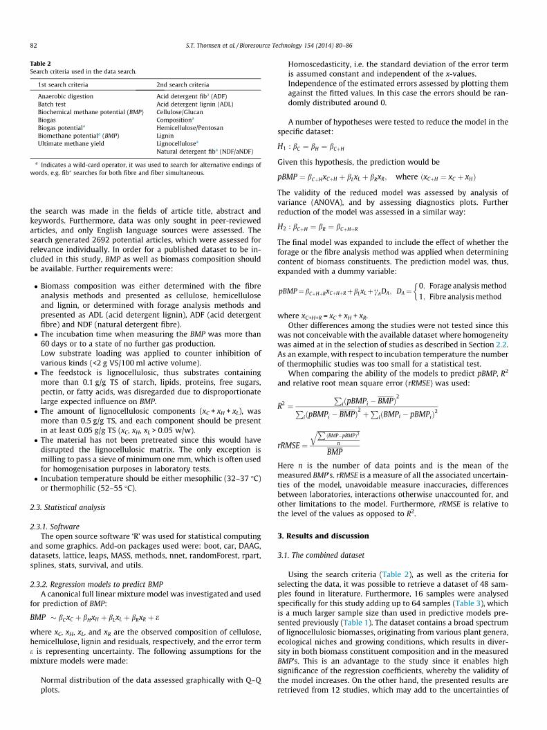
Table 2Search criteria used in the data search.

1st search criteria 2nd search criteria

Anaerobic digestion Acid detergent fiba (ADF)Batch test Acid detergent lignin (ADL)Biochemical methane potential (BMP) Cellulose/GlucanBiogas Compositiona

Biogas potentiala Hemicellulose/PentosanBiomethane potentiala (BMP) LigninUltimate methane yield Lignocellulosea

Natural detergent fiba (NDF/aNDF)

a Indicates a wild-card operator, it was used to search for alternative endings ofwords, e.g. fib⁄ searches for both fibre and fiber simultaneous.

82 S.T. Thomsen et al. / Bioresource Technology 154 (2014) 80–86

the search was made in the fields of article title, abstract andkeywords. Furthermore, data was only sought in peer-reviewedarticles, and only English language sources were assessed. Thesearch generated 2692 potential articles, which were assessed forrelevance individually. In order for a published dataset to be in-cluded in this study, BMP as well as biomass composition shouldbe available. Further requirements were:

� Biomass composition was either determined with the fibreanalysis methods and presented as cellulose, hemicelluloseand lignin, or determined with forage analysis methods andpresented as ADL (acid detergent lignin), ADF (acid detergentfibre) and NDF (natural detergent fibre).� The incubation time when measuring the BMP was more than

60 days or to a state of no further gas production.Low substrate loading was applied to counter inhibition ofvarious kinds (<2 g VS/100 ml active volume).� The feedstock is lignocellulosic, thus substrates containing

more than 0.1 g/g TS of starch, lipids, proteins, free sugars,pectin, or fatty acids, was disregarded due to disproportionatelarge expected influence on BMP.� The amount of lignocellulosic components (xC + xH + xL), was

more than 0.5 g/g TS, and each component should be presentin at least 0.05 g/g TS (xC, xH, xL > 0.05 w/w).� The material has not been pretreated since this would have

disrupted the lignocellulosic matrix. The only exception ismilling to pass a sieve of minimum one mm, which is often usedfor homogenisation purposes in laboratory tests.� Incubation temperature should be either mesophilic (32–37 �C)

or thermophilic (52–55 �C).

2.3. Statistical analysis

2.3.1. SoftwareThe open source software ‘R’ was used for statistical computing

and some graphics. Add-on packages used were: boot, car, DAAG,datasets, lattice, leaps, MASS, methods, nnet, randomForest, rpart,splines, stats, survival, and utils.

2.3.2. Regression models to predict BMPA canonical full linear mixture model was investigated and used

for prediction of BMP:

BMP � bCxC þ bHxH þ bLxL þ bRxR þ e

where xC, xH, xL, and xR are the observed composition of cellulose,hemicellulose, lignin and residuals, respectively, and the error terme is representing uncertainty. The following assumptions for themixture models were made:

Normal distribution of the data assessed graphically with Q–Qplots.

Homoscedasticity, i.e. the standard deviation of the error termis assumed constant and independent of the x-values.Independence of the estimated errors assessed by plotting themagainst the fitted values. In this case the errors should be ran-domly distributed around 0.

A number of hypotheses were tested to reduce the model in thespecific dataset:

H1 : bC ¼ bH ¼ bCþH

Given this hypothesis, the prediction would be

pBMP ¼ bCþHxCþH þ bLxL þ bRxR; where ðxCþH ¼ xC þ xHÞ

The validity of the reduced model was assessed by analysis ofvariance (ANOVA), and by assessing diagnostics plots. Furtherreduction of the model was assessed in a similar way:

H2 : bCþH ¼ bR ¼ bCþHþR

The final model was expanded to include the effect of whether theforage or the fibre analysis method was applied when determiningcontent of biomass constituents. The prediction model was, thus,expanded with a dummy variable:

pBMP¼ bCþHþRxCþHþRþbLxLþcADA; DA¼0; Forage analysis method1; Fibre analysis method

�

where xC+H+R = xC + xH + xR.Other differences among the studies were not tested since this

was not conceivable with the available dataset where homogeneitywas aimed at in the selection of studies as described in Section 2.2.As an example, with respect to incubation temperature the numberof thermophilic studies was too small for a statistical test.

When comparing the ability of the models to predict pBMP, R2

and relative root mean square error (rRMSE) was used:

R2 ¼P

iðpBMPi � BMPÞ2PiðpBMPi � BMPÞ2 þ

PiðBMPi � pBMPiÞ

2

rRMSE ¼

ffiffiffiffiffiffiffiffiffiffiffiffiffiffiffiffiffiffiffiffiffiffiffiffiffiffiffiPðBMP�pBMPÞ2

n

qBMP

Here n is the number of data points and is the mean of themeasured BMP’s. rRMSE is a measure of all the associated uncertain-ties of the model, unavoidable measure inaccuracies, differencesbetween laboratories, interactions otherwise unaccounted for, andother limitations to the model. Furthermore, rRMSE is relative tothe level of the values as opposed to R2.

3. Results and discussion

3.1. The combined dataset

Using the search criteria (Table 2), as well as the criteria forselecting the data, it was possible to retrieve a dataset of 48 sam-ples found in literature. Furthermore, 16 samples were analysedspecifically for this study adding up to 64 samples (Table 3), whichis a much larger sample size than used in predictive models pre-sented previously (Table 1). The dataset contains a broad spectrumof lignocellulosic biomasses, originating from various plant genera,ecological niches and growing conditions, which results in diver-sity in both biomass constituent composition and in the measuredBMP’s. This is an advantage to the study since it enables highsignificance of the regression coefficients, whereby the validity ofthe model increases. On the other hand, the presented results areretrieved from 12 studies, which may add to the uncertainties of

Table 3Combined dataset. Names in quotation marks specify the samples in the references.

Biomass Cellulose Hemicellulose Lignin Residual Biomethane potential ReferencexC xH xL xR BMPw/w w/w w/w w/w l CH4/kg VS

Barley straw 0.468 0.300 0.096 0.136 229 Dinuccio et al. (2010)e

Bulrush DWCa 0.361 0.210 0.150 0.279 165 Wang et al. (2010)e

Cassava stalks 0.341 0.170 0.283 0.206 101 This studyf

Clover DWC 0.263 0.183 0.142 0.412 269 Oleskowicz-Popiel et al. (2011)f

Cocoa pods 0.196 0.186 0.372 0.245 96 This studyf

Energy grass ‘Szarvasi’ DWC 0.379 0.273 0.097 0.252 322 Alaru et al. (2011)e

Foxtail millet DWC 0.330 0.316 0.053 0.300 349 Alaru et al. (2011)e

Giant reed leaves 0.331 0.185 0.245 0.239 228 Monlau et al. (2012)f

Giant reed stalks 0.209 0.177 0.254 0.360 178 Monlau et al. (2012) f

Grape stalks 0.235 0.159 0.233 0.373 98 Dinuccio et al. (2010)e

Groundnut straw 0.204 0.060 0.154 0.582 275 This studyf

Hedge cuttings 0.253 0.102 0.139 0.506 200 Triolo et al. (2011)e

Hemp ‘fibre variety’ 1 0.550 0.108 0.072 0.270 326 Alaru et al. (2011)e

Hemp ‘fibre variety’ 2 0.539 0.106 0.088 0.268 310 Alaru et al. (2011)e

Lucerne hay 0.183 0.121 0.119 0.576 276 This studyf

Maize cobs 1 0.361 0.348 0.180 0.110 339 This studyf

Maize cobs 2 0.298 0.346 0.192 0.164 228 Monlau et al. (2012)f

Maize DWC 1 0.396 0.195 0.079 0.330 363 This studyf

Maize DWC 2b 0.224 0.269 0.061 0.446 311 Oslaj et al. (2010)e

Maize DWC 3c 0.266 0.287 0.075 0.372 319 Oslaj et al. (2010)e

Maize DWC 4d 0.318 0.284 0.071 0.327 288 Oslaj et al. (2010)e

Maize leaves 0.309 0.286 0.204 0.201 257 Monlau et al. (2012)f

Maize stalks 1 0.384 0.219 0.170 0.227 333 This studyf

Maize stalks 2 0.271 0.212 0.232 0.285 206 Monlau et al. (2012)f

Maize stalks 3 0.301 0.190 0.103 0.406 360 Tong et al. (1990)f

Miscanthus DWC 0.420 0.302 0.070 0.209 349 Alaru et al. (2011)e

Napier grass DWC 0.360 0.187 0.105 0.348 288 Tong et al. (1990)f

Oil palm EFB 0.335 0.230 0.238 0.197 189 This studyf

Perennial grass DWC 0.291 0.260 0.058 0.392 271 Triolo et al. (2011)e

Plantain leaves 0.225 0.202 0.183 0.390 207 This studyf

Plantain trunks 0.463 0.138 0.124 0.275 275 This studyf

Rice straw 1 0.339 0.204 0.113 0.344 327 This studyf

Rice straw 2 0.262 0.188 0.270 0.280 217 Monlau et al. (2012)f

Rice straw 3 0.334 0.282 0.074 0.310 360 He et al. (2008)e

Rye DWC 0.500 0.182 0.107 0.211 417 Oleskowicz-Popiel et al. (2011)f

Rye straw 1 0.365 0.240 0.177 0.218 220 This studyf

Rye straw 2 0.408 0.246 0.193 0.153 297 This studyf

Smooth cordgrass DWC 0.340 0.299 0.097 0.264 358 Triolo et al. (2011)e

Sorghum ‘Akklimat’ 0.309 0.232 0.055 0.404 232 Mahmood and Honermeier (2012)e

Sorghum ‘Biomass variety’ 0.222 0.194 0.214 0.370 250 Monlau et al. (2012)f

Sorghum ‘Bovital’ 1 0.296 0.199 0.045 0.460 302 Mahmood and Honermeier (2012)e

Sorghum ‘Bovital’ 2 0.292 0.223 0.045 0.440 282 Mahmood and Honermeier (2012)e

Sorghum ‘Forage variety’ 0.183 0.217 0.207 0.393 280 Monlau et al. (2012)f

Sorghum ‘Goliath’ 1 0.363 0.199 0.053 0.385 320 Mahmood and Honermeier (2012)e

Sorghum ‘Goliath’ 2 0.334 0.193 0.053 0.420 280 Mahmood and Honermeier (2012)e

Sorghum stalks ‘Seed variety’ 0.291 0.261 0.225 0.223 236 Monlau et al. (2012)f

Sorghum ‘Sweet variety’ 1 0.201 0.209 0.185 0.405 314 Monlau et al. (2012)f

Sorghum ‘Sweet variety’ 2 0.197 0.200 0.198 0.405 307 Monlau et al. (2012)f

Sorghum ‘Sweet variety’ 3 0.181 0.185 0.213 0.421 289 Monlau et al. (2012)f

Sunflower stalks 1 0.310 0.156 0.292 0.242 185 Monlau et al. (2012)f

Sunflower stalks 2 0.312 0.143 0.277 0.268 190 Monlau et al. (2012)f

Sunflower stalks 3 0.312 0.143 0.300 0.245 183 Monlau et al. (2012)f

Sunflower stalks bark 0.274 0.135 0.350 0.241 161 Monlau et al. (2012)f

Vetch hay 0.293 0.164 0.214 0.328 191 This studyf

Vetch hay and rye straw 1 0.336 0.219 0.185 0.259 236 This studyf

Vetch hay and rye straw 2 0.364 0.225 0.193 0.218 236 This studyf

Wheat straw 1 0.480 0.284 0.064 0.172 290 Triolo et al. (2011)e

Wheat straw 2 0.490 0.340 0.065 0.105 208 Sambusiti et al. (2012)f

Wheat straw 3 0.337 0.186 0.174 0.303 302 Tong et al. (1990)f

Wheat straw 4 0.350 0.182 0.172 0.296 333 Tong et al. (1990)f

Wild grass DWC 0.360 0.229 0.060 0.351 306 Triolo et al. (2011)e

Wild plants 0.337 0.229 0.101 0.333 214 Triolo et al. (2012)e

Wood cuttings 0.224 0.120 0.225 0.431 172 Triolo et al. (2012)e

Wood grass 0.390 0.149 0.273 0.188 291 Tong et al. (1990)f

a DWC = dried whole crop.b Average of different hybrids at maturity class FAO 500–600 (mature).c Average of different hybrids at maturity class FAO 400–500 (less mature).d Average of different hybrids at maturity class FAO 300–400 (young).e Indicates for age method used for biomass composition analysis.f Indicates fiber method used for biomass composition analysis.

S.T. Thomsen et al. / Bioresource Technology 154 (2014) 80–86 83

Theoretical quantiles

Obs

erve

d qu

antil

es

Fitted values

Erro

rs

(a) (b)

Fig. 1. (a) A normal Q–Q plot of the derived model (pBMP = 378 xC + 354 xH � 194 xL +313 xR). (b) Errors vs. fitted values from the same model.

84 S.T. Thomsen et al. / Bioresource Technology 154 (2014) 80–86

the results, e.g. due to differences in the laboratory proceduresapplied.

3.2. Regression models to predict BMP

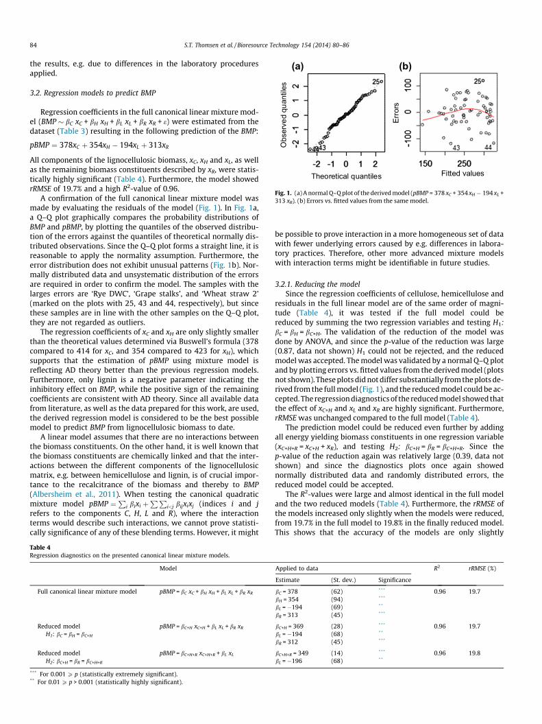
Regression coefficients in the full canonical linear mixture mod-el (BMP � bC xC + bH xH + bL xL + bR xR + e) were estimated from thedataset (Table 3) resulting in the following prediction of the BMP:

pBMP ¼ 378xC þ 354xH � 194xL þ 313xR

All components of the lignocellulosic biomass, xC, xH and xL, as wellas the remaining biomass constituents described by xR, were statis-tically highly significant (Table 4). Furthermore, the model showedrRMSE of 19.7% and a high R2-value of 0.96.

A confirmation of the full canonical linear mixture model wasmade by evaluating the residuals of the model (Fig. 1). In Fig. 1a,a Q–Q plot graphically compares the probability distributions ofBMP and pBMP, by plotting the quantiles of the observed distribu-tion of the errors against the quantiles of theoretical normally dis-tributed observations. Since the Q–Q plot forms a straight line, it isreasonable to apply the normality assumption. Furthermore, theerror distribution does not exhibit unusual patterns (Fig. 1b). Nor-mally distributed data and unsystematic distribution of the errorsare required in order to confirm the model. The samples with thelarges errors are ‘Rye DWC’, ‘Grape stalks’, and ‘Wheat straw 2’(marked on the plots with 25, 43 and 44, respectively), but sincethese samples are in line with the other samples on the Q–Q plot,they are not regarded as outliers.

The regression coefficients of xC and xH are only slightly smallerthan the theoretical values determined via Buswell’s formula (378compared to 414 for xC, and 354 compared to 423 for xH), whichsupports that the estimation of pBMP using mixture model isreflecting AD theory better than the previous regression models.Furthermore, only lignin is a negative parameter indicating theinhibitory effect on BMP, while the positive sign of the remainingcoefficients are consistent with AD theory. Since all available datafrom literature, as well as the data prepared for this work, are used,the derived regression model is considered to be the best possiblemodel to predict BMP from lignocellulosic biomass to date.

A linear model assumes that there are no interactions betweenthe biomass constituents. On the other hand, it is well known thatthe biomass constituents are chemically linked and that the inter-actions between the different components of the lignocellulosicmatrix, e.g. between hemicellulose and lignin, is of crucial impor-tance to the recalcitrance of the biomass and thereby to BMP(Albersheim et al., 2011). When testing the canonical quadraticmixture model pBMP ¼

Pi bixi þ

PPi<j bijxixj (indices i and j

refers to the components C, H, L and R), where the interactionterms would describe such interactions, we cannot prove statisti-cally significance of any of these blending terms. However, it might

Table 4Regression diagnostics on the presented canonical linear mixture models.

Model

Full canonical linear mixture model pBMP = bC xC + bH xH + bL xL + bR xR

Reduced modelH1: bC = bH = bC+H

pBMP = bC+H xC+H + bL xL + bR xR

Reduced modelH2: bC+H = bR = bC+H+R

pBMP = bC+H+R xC+H+R + bL xL

*** For 0.001 P p (statistically extremely significant).** For 0.01 P p > 0.001 (statistically highly significant).

be possible to prove interaction in a more homogeneous set of datawith fewer underlying errors caused by e.g. differences in labora-tory practices. Therefore, other more advanced mixture modelswith interaction terms might be identifiable in future studies.

3.2.1. Reducing the modelSince the regression coefficients of cellulose, hemicellulose and

residuals in the full linear model are of the same order of magni-tude (Table 4), it was tested if the full model could bereduced by summing the two regression variables and testing H1:bC = bH = bC+H. The validation of the reduction of the model wasdone by ANOVA, and since the p-value of the reduction was large(0.87, data not shown) H1 could not be rejected, and the reducedmodel was accepted. The model was validated by a normal Q–Q plotand by plotting errors vs. fitted values from the derived model (plotsnot shown). These plots did not differ substantially from the plots de-rived from the full model (Fig. 1), and the reduced model could be ac-cepted. The regression diagnostics of the reduced model showed thatthe effect of xC+H and xL and xR are highly significant. Furthermore,rRMSE was unchanged compared to the full model (Table 4).

The prediction model could be reduced even further by addingall energy yielding biomass constituents in one regression variable(xC+H+R = xC+H + xR), and testing H2: bC+H = bR = bC+H+R. Since thep-value of the reduction again was relatively large (0.39, data notshown) and since the diagnostics plots once again showednormally distributed data and randomly distributed errors, thereduced model could be accepted.

The R2-values were large and almost identical in the full modeland the two reduced models (Table 4). Furthermore, the rRMSE ofthe models increased only slightly when the models were reduced,from 19.7% in the full model to 19.8% in the finally reduced model.This shows that the accuracy of the models are only slightly

Applied to data R2 rRMSE (%)

Estimate (St. dev.) Significance

bC = 378 (62) *** 0.96 19.7bH = 354 (94) ***

bL = �194 (69) **

bR = 313 (45) ***

bC+H = 369 (28) *** 0.96 19.7bL = �194 (68) **

bR = 312 (45) ***

bC+H+R = 349 (14) *** 0.96 19.8bL = �196 (68) **

S.T. Thomsen et al. / Bioresource Technology 154 (2014) 80–86 85

reduced compared to the full model. Therefore, based on this set ofdata, the reduced model, H2 seems adequate.

For design of future predictions models, it is important to startagain from the full model and not from a reduced model since thereduction depends on estimated regression coefficients, and in adifferent dataset, the coefficients will have different numericalvalues reflecting the type of biomass. In addition, models basedon biomasses with other characteristics, such as high content oflipids or proteins, should include regression coefficients reflectingthis fact. For design of future models, it might also be appropriateto use more advanced mixture model as developed for thechemical and pharmaceutical fields, see e.g. (Focke et al., 2007;Mandlik Satish et al., 2012).

3.2.2. Comparison to previous modelsThe inherent mathematical relation between canonical linear

mixture models and models with intercept as applied previouslyis exemplified by the following calculations:

bCxC þ bHxH þ bLxL þ bRxR

¼ bCxC þ bHxH þ bLxL

þ bRð1� xC � xH � xLÞ¼ ðbC � bRÞxC þ ðbH � bRÞxH þ ðbL � bRÞxL þ bR

¼ a0 þ aCxC þ aHxH þ aLxL;

wherea0 ¼ bR;aC ¼ bC � bR;aH ¼ bH � bR; and aL ¼ bL � bR

Therefore, it is possible to mathematically transform regressioncoefficients from one to another manner of expressing the model.However, the regression coefficients would not necessarily makeintuitive sense. For example, if bC and bR are both positive and ofthe same order of magnitude then aC = bC � bR will be small, thusseemingly insignificant. If bC < bR, the sign will be negative eventhough this is contrary to AD theory. This was the case with the pre-diction model proposed by Triolo et al. (2011) (Table 1):

pBMP ¼ 447� 277xL � 7xC :

Further, since bL is a negative regression coefficient, aL = bL � bR maybe even more negative and, thereby, highly significant. Thus,the role of lignin may previously have been exaggerated; notnecessarily in the statistical calculations, but also in the way weunderstand and interpret previous results.

Predictions based on our model H2, pBMP = bC+H+R xC+H+R + bL xL,can be recalculated similarly into a0 + aL xL, where, a0 = bC+H+R andaL = bL � bC+H+R. In this notation, pBMP = 348 � 544 xL is the sameas the model previously proposed by both Triolo et al. (2011)and Monlau et al. (2012) (Table 1). Comparing our regression coef-ficients to those previously published (Table 1), our effect of ligninis more negative. It should be noted that the previously publishedregression coefficients are determined on homogeneous biomassesand on quite small sample-sizes, and apparently, they are notapplicable for describing pBMP from lignocellulosic biomass ingeneral.

Table 5Regression diagnostics on the alternative models.

Model

Including dummy-variable regressor for analysis method pBMP = bC+H+R xC+H+R + b

DA ¼0 Forage meth1 Fiber metho

�

*** For 0.001 P p (statistically extremely significant).

3.2.3. Effect of biomass analysis methodAmong the factors affecting the outcome of BMP measurements,

using the forage or the fibre method for analysing biomass compo-sition turned out to be of large importance especially for the lignincontent (Table 3). We estimated a statistically highly significant ef-fect of whether the compositional data was generated with eitherof the two methods (Table 5). This indicates that the two methodsdo not generate fully comparable results, and thus when determin-ing pBMP it is important to know which of the methods had beenused in the specific case. The dummy variable seems to be relatedto the lignin content as the bL changes very much when the dum-my variable is introduced while bC+H+R stays unchanged. The effectthat pBMP is 63 units larger, when the fibre method has been ap-plied compared to when the forage method has been applied, couldbe explained by that the fibre method estimates a higher lignincontent compared to the forage method. In this case, predictionsmade by means of the fibre method, which results in a larger neg-ative contribution to pBMP, will be compensated by the dummyvariable. R2 is increased while rRMSE is decreased compared tothe final reduced model. In addition, the diagnostics plots con-firmed normal distribution of the data as well as independenceof the residuals (data not shown).

3.3. Limitations of the study

Some factors expected to influence BMP were not taken into ac-count in the statistical analysis and this may have affected the out-come of the study. Among these factors are:

Activity, activation and adaptation of the inoculum for BMPmeasurements. These factors have been shown to have a large im-pact on BMP (Gerber et al., 2013).

� End-point inaccuracy and various inhibitions of the BMPmeasurements.� Deviating laboratory practices when determining BMP, such as

biomass particle size, mixing, and incubation temperature.� Additional differences in determination of biomass constituents

other than fibre vs. forage method.

These factors most likely account for a large part of the variationin the dataset. This might have been avoided if more strict criteriafor selecting data were applied. However, a large dataset with abroad variety of lignocellulosic biomasses were prioritised on theexpense of presumable larger variation. In future studies, a predic-tion based on a large dataset from strictly standardised laboratoryprocedures, would presumably result in regression coefficientswith lower standard deviation. In addition, it would be beneficialwith a more thorough biomass composition analysis, where otherbiomass constituents also were accounted for.

An indication of deviating data in this study can be seen whencomparing composition of rice straw compiled in this article. Ricestraw 1 and Rice straw 2 were analysed with the fibre analysismethod but their lignin content was very different (0.113 and0.270 w/w, respectively). This might be a result of large naturalvariation, but it is likely also to be influenced by differences in

Applied to data R2 rRMSE

Estimate (St. dev.) Significance

L xL + cA DA bC+H+R = 347 (13) *** 0.97 17.7%bL = �438 (87) ***od

d cA = 63 (16) ***

86 S.T. Thomsen et al. / Bioresource Technology 154 (2014) 80–86

laboratory practices. Likewise, the data from Triolo et al. (2011)had unusually low lignin contents. These samples were analysedwith the forage analysis, however, the low lignin values might alsobe a result of other specific practices used in that study. Eventhough a dummy variable was included in our model to describethe two different analysis methods, the difference between differ-ent research groups were not assessed.

Further, variation in the nature of the biomass constituents hasnot been taken into account. Hemicelluloses differ according to thebiomass in question, in respect to both structural backbone andside chains, and likewise the exact structure of lignin can vary fromone biomass to the other (Albersheim et al., 2011). Due to theavailability of data, this has not been assessed in the current study.

Finally, it should be noticed that some biomasses commonlyused for biogas production are omitted from the dataset due tothe criteria of selecting the data. For instance, ensiled biomasseswere excluded on beforehand due to a presumed large amount offatty acids. Likewise, waste residues important for AD, such asmanure, starchy materials, marine biomass, household waste, orindustrial wastes, were omitted. In future studies, these biomassesmay also be addressed, either individually or combined. The corre-sponding mixture model for predicting BMP should include thepredominant biomass constituents as explanatory variables, in or-der to test the significance of the estimated regression coefficients.

4. Conclusion

Using canonical linear mixture models instead of standard lin-ear regression models to predict BMP provides highly significantregression coefficients for the different biomass constituents inaccordance with AD theory. Based on the large dataset (n = 64),the following equation to predict BMP was developed:

pBMP ¼ 378xC þ 354xH � 194xL þ 313xR:

It was possible to reduce this model while including a dummy var-iable for the biomass composition analysis method without losingvalidity of the model:

pBMP¼347xCþHþR�438xLþ63DA; DA0; Forage analysis method1; Fibre analysis method

�

Furthermore, it is suggested that prediction of BMP in future studieswith other types of biomasses should also be carried out usingmixture models.

Acknowledgements

This work was supported with a grant from Danida FellowshipCentre (DFC) of the Danish Ministry of Foreign Affairs, as a part ofthe project ‘‘Biofuel production from lignocellulosic materials –2GBIONRG’’, DFC journal no. 10-018RISØ. For additional informa-tion, see http://2gbionrg.dk. P. Kroff is recognized for his valuableinitial inputs. H. Carrere is acknowledged for providing additionaldata to enable use of the reference by Monlau et al. (2012).

References

Alaru, M., Olt, J., Kukk, L., Luna-delRisco, M., Lauk, R., Noormets, M., 2011. Methaneyield of different energy crops grown in Estonian conditions. J. Agric. Res. 9, 13–22.

Albersheim, P., Darvillis, A., Robertsis, K., Sederoffis, R., Staehelinis, A., 2011. PlantCell Walls: From Chemistry to Biology. Taylor & Francis Group.

Angelidaki, I., Alves, M., Bolzonella, D., Borzacconi, L., Campos, J.L., Guwy, A.J.,Kalyuzhnyi, S., Jenicek, P., Van Lier, J.B., 2009. Defining the biomethane potential(BMP) of solid organic wastes and energy crops: a proposed protocol for batchassays. Water Sci. Technol. 59, 927–934.

Azhar, N.G., Stuckey, D.C., 1994. The influence of chemical structure on theanaerobic catabolism of refractory compounds: a case study of instant coffeewastes. Water Sci. Technol. 30, 223–232.

Carter, M.S., Hauggaard-Nielsen, H., Heiske, S., Jensen, M., Thomsen, S.T., Schmidt,J.E., Johansen, A., Ambus, P., 2012. Consequences of field N2O emissions for theenvironmental sustainability of plant-based biofuels produced within anorganic farming system. GCB Bioenergy 4, 435–452.

Cornell, J.A., 2011. A retrospective view of mixture experiments. Qual. Eng. 23, 315–331.

Dinuccio, E., Balsari, P., Gioelli, F., Menardo, S., 2010. Evaluation of the biogasproductivity potential of some Italian agro-industrial biomasses. Bioresour.Technol. 101, 3780–3783.

Focke, W.W., Sandrock, C., Kok, S., 2007. Weighted-power-mean mixture model:application to multicomponent liquid viscosity. Ind. Eng. Chem. Res. 46, 4660–4666.

Gerber, M., Schneider, N., Kowalczyk, A., Schwede, S., Rehman, Z., Span, R., 2013. Theinfluence of pre-incubation, storage and homogenization of inoculum for batchtests on biogas production.

Gunaseelan, V.N., 2007. Regression models of ultimate methane yields of fruits andvegetable solid wastes, sorghum and napiergrass on chemical composition.Bioresour. Technol. 98, 1270–1277.

Gunaseelan, V.N., 2009. Predicting ultimate methane yields of Jatropha curcus andMorus indica from their chemical composition. Bioresour. Technol. 100, 3426–3429.

Hansen, T.L., Schmidt, J.E., Angelidaki, I., Marca, E., Jansen, J.l.C., Mosbæk, H.,Christensen, T.H., 2004. Method for determination of methane potentials ofsolid organic waste. Waste Manage. 24, 393–400.

He, Y., Pang, Y., Liu, Y., Li, X., Wang, K., 2008. Physicochemical characterization ofrice straw pretreated with sodium hydroxide in the solid state for enhancingbiogas production. Energy Fuel. 22, 2775–2781.

Labatut, R.A., Angenent, L.T., Scott, N.R., 2011. Biochemical methane potential andbiodegradability of complex organic substrates. Bioresour. Technol. 102, 2255–2264.

Mahmood, A., Honermeier, B., 2012. Chemical composition and methane yield ofsorghum cultivars with contrasting row spacing. Field Crop. Res. 128, 27–33.

Mandlik Satish, K., Saugat, A., Deshpande Ameya, A., 2012. Application of simplexlattice design in formulation and development of buoyant matrices ofdipyridamole. J. Appl. Pharm. Sci. 2, 107–111.

Monlau, F., Sambusiti, C., Barakat, A., Guo, X.M., Latrille, E., Trably, E., Steyer, J.-P.,Carrere, H., 2012. Predictive models of biohydrogen and biomethane productionbased on the compositional and structural features of lignocellulosic materials.Environ. Sci. Technol. 46, 12217–12225.

Oleskowicz-Popiel, P., Thomsen, A.B., Schmidt, J.E., 2011. Ensiling - Wet-storagemethod for lignocellulosic biomass for bioethanol production. BiomassBioenerg. 35, 2087–2092.

Oslaj, M., Mursec, B., Vindis, P., 2010. Biogas production from maize hybrids.Biomass Bioenerg. 34, 1538–1545.

Prakasham, R.S., Sathish, T., Brahmaiah, P., Subba Rao, C., Sreenivas Rao, R., Hobbs,P.J., 2009. Biohydrogen production from renewable agri-waste blend:optimization using mixer design. Int. J. Hydrogen Energy 34, 6143–6148.

Sambusiti, C., Ficara, E., Rollini, M., Manzoni, M., Malpei, F., 2012. Sodium hydroxidepretreatment of ensiled sorghum forage and wheat straw to increase methaneproduction. Water Sci. Technol. 66, 2447–2452.

Scheffe, H., 1963. The simplex-centroid design for experiments with mixtures. J. R.Stat. Soc. B Met. 25, 235–263.

Sluiter, J.B., Ruiz, R.O., Scarlata, C.J., Sluiter, A.D., Templeton, D.W., 2010.Compositional analysis of lignocellulosic feedstocks. 1. Review anddescription of methods. J. Agric. Food Chem. 58, 9043–9053.

Symons, G.E., Buswell, A.M., 1933. The methane fermentation of carbohydrates. J.Am. Chem. Soc. 55, 2028–2036.

Thomsen, S.T., Jensen, M., Schmidt, J.E., 2012. Production of 2nd generationbioethanol from lucerne – optimization of hydrothermal pretreatment.BioResource 7, 1582–1593.

Tong, X., Smith, L.H., McCarty, P.L., 1990. Methane fermentation of selectedlignocellulosic materials. Biomass 21, 239–255.

Triolo, J.M., Sommer, S.G., Møller, H.B., Weisbjerg, M.R., Jiang, X.Y., 2011. A newalgorithm to characterize biodegradability of biomass during anaerobicdigestion: influence of lignin concentration on methane production potential.Bioresour. Technol. 102, 9395–9402.

Triolo, J.M., Pedersen, L., Qu, H., Sommer, S.G., 2012. Biochemical methane potentialand anaerobic biodegradability of non-herbaceous and herbaceous phytomassin biogas production. Bioresour. Technol. 125, 226–232.

Wang, J., Yue, Z., Chen, T., Peng, S., Yu, H., Chen, H., 2010. Anaerobic digestibility andfiber composition of bulrush in response to steam explosion. Bioresour. Technol.101, 6610–6614.