General rights Copyright and moral rights for the publications made accessible in the public portal are retained by the authors and/or other copyright owners and it is a condition of accessing publications that users recognise and abide by the legal requirements associated with these rights.

Users may download and print one copy of any publication from the public portal for the purpose of private study or research.

You may not further distribute the material or use it for any profit-making activity or commercial gain

You may freely distribute the URL identifying the publication in the public portal If you believe that this document breaches copyright please contact us providing details, and we will remove access to the work immediately and investigate your claim.

Downloaded from orbit.dtu.dk on: Apr 05, 2020

Statistical prediction of parametric roll using FORM

Jensen, Jørgen Juncher; Choi, Ju-hyuck; Nielsen, Ulrik Dam

Published in:Ocean Engineering

Link to article, DOI:10.1016/j.oceaneng.2017.08.029

Publication date:2017

Document VersionPeer reviewed version

Link back to DTU Orbit

Citation (APA):Jensen, J. J., Choi, J., & Nielsen, U. D. (2017). Statistical prediction of parametric roll using FORM. OceanEngineering, 144, 235–242. https://doi.org/10.1016/j.oceaneng.2017.08.029

Statistical prediction of parametric roll using FORM

Jørgen Juncher Jensen1, Ju-hyuck Choi1, Ulrik Dam Nielsen1,2

1Department of Mechanical Engineering, Technical University of Denmark, Kgs. Lyngby, Denmark 2Centre for Autonomous Marine Operations and Systems (AMOS), Dept. of Marine Tech., NTNU, Trondheim, Norway

ABSTRACT

Previous research has shown that the First Order Reliability Method (FORM) can be an efficient method for estimation of outcrossing rates and extreme value statistics for stationary stochastic processes. This is so also for bifurcation type of processes like parametric roll of ships. The present paper discusses this solution procedure with a focus on the computational efficiency of FORM as compared with Monte Carlo Simulation (MCS).

KEY WORDS Parametric roll; FORM; mean out-crossing rate, reliability index, critical wave episodes

INTRODUCTION Currently, extensive work is going on within the International Maritime Organization (IMO) in the development of Second Generation Intact Stability Criteria for ships. These completely revised rules include the possibility to account for the dynamics of ships using time-domain simulations of the roll motion under different operational conditions, considering different failure scenarios (pure loss of stability, parametric roll, dead ship, excessive acceleration and surf riding / broaching) and involve different levels of complexity and corresponding accuracy. Tompuri et al. (2015) discuss in details computational methods to be used in the Second Generation Intact Stability Criteria, focussing on level 1 and level 2 procedures for parametric roll, pure loss of stability and surf-riding/broaching. These methods are based on the analysis of the ship in regular waves with different wave height and thus do not directly provide extreme value statistics.

The rules might not only be used in the design phase, but also be needed under operation as GM limit curves cannot always be formulated using the new rules, e.g. IMO (2017). For the more detailed analyses in Level 3, and for operational guidelines/limitations, a direct account for the statistical properties of the ocean waves will be needed and so will effective statistical estimation procedures to cover the full operational profile of a vessel.

France et al. (2003) present an excellent and very thorough description of the physics in parametric roll; with discussions based on both numerical studies and model test results. Hence, the present paper will focus on an extreme value prediction procedure applicable as an extension to more deterministic formulations of parametric roll.

The First Order Reliability Method (FORM) is an efficient procedure for extreme value predictions for time-invariant stochastic processes, e.g. Der Kiureghian (2000), Jensen and Capul (2006), Jensen

(2015). Jensen (2007) uses FORM for estimation of the probability of parametric roll. In the present paper the same one degree-of-freedom formulation of parametric roll is used, but two simple and effective optimization procedures, easy to implement in any time-domain code for FORM evaluations, are presented. Furthermore, some characteristic response behaviour in parametric roll is discussed. A recent study by Choi et al. (2017) gives a somewhat similar treatment of intact stability under dead ship conditions.

FIRST ORDER RELIABILITY PROCEDURES The basic assumption for the application of the FORM method herein is that the response can be considered as a stationary time-domain process, depending solely on a load process in time t and space X, defined in terms of some deterministic quantities and a set of statistical independent and standard normal distributed variables { }, ; 1,2,..,i iu u u i n= = . For wave responses, the long-crested wave elevation process ( , )H X t is such a process, e.g. Jensen and Capul (2006):

( )1

( , ) ( , ) ( , )n

i i i ii

H X t u c X t u c X t=

= +∑ (0)

where the deterministic coefficients are

2( , ) cos( ); ( , ) sin( ); ( )i i i i i i i i i i ic x t t k X c x t t k X S ds ω s ω s ω ω= − = − − = (0)

Here iω and 2 /i ik gω= are the n discrete frequencies and wave numbers applied, respectively. Furthermore, g is the acceleration of gravity, ( )S ω is the wave spectrum and, idω is the increment between the discrete frequencies. Stochastic wind speed can also be modelled in a similar way, e.g. Choi et al. (2017).

For a set of u , the wave elevation is used as input to a time-domain formulation for the response ( , )t uφ . Due to the assumption of a stationary stochastic process, the response at any point in time

0t t= can be applied in the limit state function

( )0 0( ) , 0G u t uφ φ= − = (0)

without changing the result for the probability of exceedance at a given threshold response level 0φ . The only restriction is that the point in time 0t chosen must be so far away from the initial conditions that these do not influence the response. For parametric roll 300s was found in Jensen (2007) to be sufficient. For other wave responses 60s might be sufficient, e.g. Jensen (2015).

The main part of any FORM procedure is an optimization routine for determination of the point *uon the limit state function ( ) 0G u = with the shortest distance from origin. The distance to this point is denoted the reliability index β . Two optimization routines: 1) A modified Hasofer-Lind procedure (MHL) and, 2) the Hasofer-Lind method supplemented with a circle and line search (CLS) are used here.

In the original Hasofer-Lind iteration procedure, Hasofer and Lind (1974), a new iteration point 1ku + is determined from the previous point ku as

[ ]1 2

( )( ) ( )( )

kk k k k k

k

G uu a G u u G uG u+

∇= = ∇ −

∇ (0)

Here ∇ is the gradient operator and the length of the vector. However, for the problems

considered here, this procedure does not generally converge towards the design point *u . This lack of robustness of the Hasofer-Lind procedure is discussed in details in Liu and Der Kiureghian (1991) and several remedies are suggested.

In the Modified Hasofer-Lind method, Liu and Der Kiureghian (1991), the new iteration point

1ku + is determined from a line search along the line:

( )1k ku a uς ς= + − (0)

where ka is given by Eq. (4). The scalar ς is determined by a simple stepping procedure until the

merit function ( )m u

[ ]22

2( )( ) ( ) ( )( )

G u um u u G u G uG u

c ∇

= − ∇ ∇

+ (0)

attains a minimum value, yielding

( ){ }1 minku u m uς+ = = (0)

The weight factor c can be taken in a wide range from 1,000 to 10,000 without changing the convergence significantly for the present problems, where the response 0φ in the limit state function, Eq. (3), is the roll angle in radians. This insensitivity of convergence rate with c is in agreement with the findings in Liu and Der Kiureghian (1991) considering very different examples. The range investigated for ς is ] ]0,2ς ∈ with a step size of 0.025. The procedure is very easy to

implement and convergence is found in all cases considered here. The procedure is, however, rather CPU expensive as it requires gradient calculations ( )G u∇ for all values of ς used in Eq. (5).

An alternative is the Hasofer-Lind procedure supplemented with a circle and line search, Choi et al. (2017). Based on the previous iteration step ku the new iteration point 1ku + is determined from first a circle search along the circle:

( ) ( )( )11

kk k

k k

au a u

a uς ς

ς ς= + −

+ − (0)

where ka is given by Eq. (4). The scalar ς is determined by a simple stepping procedure until

the limit state function ( )G u attains a minimum value. The corresponding value of u is denoted

u . Thereafter a line search along the line u uξ= is performed. The scalar ξ is determined such that ( ) 0G u = yielding

{ }1 ( ) 0ku u G uξ

ξ ξ+ = = (0)

A Newton-Raphson approach is applied based on previous values at iteration step i and i-1:

11

1( )

( ) ( )i i

i iii i

G uG u G u

ξ ξξ ξ ξξ ξ

−+

−

−= −−

(0)

For the first step, 1 1 0.01 ( ) / eG u Gξ = + is found useful. Here, eG is the user-defined convergence

criterion for the limit state function. With the threshold angles 0φ measured in radians,

0.002eG = has been found adequate.

The convergence property of this scheme is just as good as for the MHL procedure, in all cases considered, and the scheme provides a large reduction of CPU time although the number of iteration steps generally is larger. The reason is that gradient calculations are not needed during the circle–and-line search as opposite to the MHL method. With a large number of components in u , say 100 as used later in the next example, the CPU time is thereby reduced by a factor of three to five. Both procedures, however, converge for all cases tested to the same design point *u u= .

The distance to the design point *u is the reliability index β and from it extreme value predictions can easily be obtained, e.g. Jensen and Capul (2006),

( )20 0 0max (t) 1 exp exp( 0.5 ( ) )

TP v Tφ φ β φ

> = − − − (0)

Here T is the time period considered, e.g. three hours, and 0ν the mean zero- upcrossing rate, roughly equal to the roll natural frequency in Hz. It should, however, be noted that Eq. (11) does not account for possible grouping of the threshold angles. This is not investigated here, where the focus is on comparison between reliability indices from FORM and MSC, but the procedure suggested by Naess and Gaidai (2009) could for instance be implemented in the time domain simulations to account for the clustering effect. Thereby, Eq.(11) is replaced by a somewhat similar expression, Naess and Gaidai (2009).

EFFECTIVE WAVE FOR GZ CALCULATIONS Parametric roll in head sea depends on the variation of the instantaneous GZ curve in waves. In principle the roll restoring moment can be calculated at each point in time, e.g. Vidic-Perunovic and Jensen (2009), but this is computationally expensive. Therefore it is often estimated by interpolation in predefined GZ curves derived from hydrostatic results with the ship ‘resting’ in regular waves with a wave length equal to the length L of the vessel. The wave height ( )h t and wave crest

position ( )cx t used in this interpolation are found by a least square approximation to the incident wave ( , )H X t , Eqs. (1)-(2), cf. Jensen (2007):

( )( ) ( )( )( ) ( )

0 0

2 2

2 2 2 2( ) , , cos ; ( ) , , sin

, cos

( ) 2

2 ( )arccos if ( ) 02 ( )

( )2 ( )arccos if ( ) 0

2 ( )

( ) ( )

e eL L

e e e e

e

ce

e

x xa t H X x t t dx b t H X x t t dxL L L L

X x t x Vt

h t a b

L a t b th t

x tL a tL b t

h t

t t

π π

c

π

π

= =

= +

= +

>=

− <

∫ ∫

(0)

Here eL is an effective wave length used in the analytical approximation for the GZ curve in waves. In Jensen (2007), the calculations of the two integrals were performed numerically using Gaussian Quadrature at every time step. However, due to the sinusoidal form of Eq. (1), analytical integration can be carried out, resulting in a significant decrease in computational time:

0 1 2 0 1 21 1

0 02 2 2 2

1 2

/ 2

( ) cos( ) sin( ) ; ( ) sin( ) cos( )

2 sin 2 sin;

cos sin ; sin coscos( ); cos( ); ei e

n n

i i i ii i i i i ii i

i ii i

i i i ii i

i i i ei i k L

a t a v t v t b t b v t v t

a b

v u u v u uk V k k

ω ω ω ω

µ µ π µs sµ π µ πµ µ µ µ

ω ω c c µ

= = = + = −

= =− −

= + = −= − = =

∑ ∑

(0)

Here c is the heading angle (180 degree for head sea) and V the forward speed. It is seen that ( )a t is the original Grim wave, Grim (1961), with the wave crest assumed always amidships. The

inclusion of ( )b t makes estimation of the instantaneous wave crest position possible.

FIRST ORDER RELIABILITY RESULTS FOR PARAMETRIC ROLL

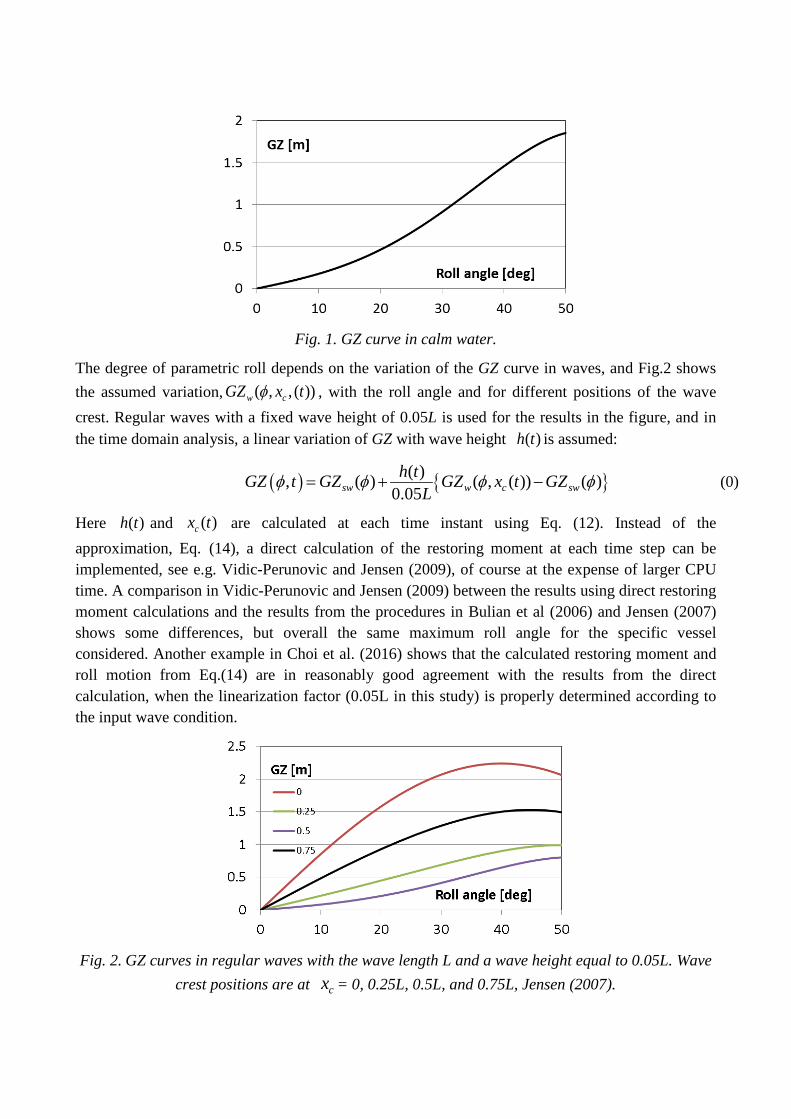
The analysis is done for the same Panamax container ship and operational data as in Jensen (2007). The length, breadth and draft of the vessel are L = 284m, B = 32.2m and 10.5m, respectively. The operational condition is head sea with a forward speed of 6m/s and a sea state characterized by a JONSWAP spectrum with significant wave height SH = 12m and a wave spectral peak period of 15s. This is of course a very severe sea state, but chosen such that MCS are possible with reasonable CPU time even for large threshold angles. Later a moderate sea state will be considered. The metacentric height GM = 0.89m and the GZ curve, ( )swGZ φ , in calm water is shown in Fig. 1 as function of the roll angle φ . With a ship speed of 6m/s, the encounter spectral wave peak period becomes 12s and hence parametric roll can be expected.

Fig. 1. GZ curve in calm water.

The degree of parametric roll depends on the variation of the GZ curve in waves, and Fig.2 shows the assumed variation, ( , , ( ))w cGZ x tφ , with the roll angle and for different positions of the wave crest. Regular waves with a fixed wave height of 0.05L is used for the results in the figure, and in the time domain analysis, a linear variation of GZ with wave height ( )h t is assumed:

( ) { }( ), ( ) ( , ( )) ( )0.05sw w c swh tGZ t GZ GZ x t GZ

Lφ φ φ φ= + − (0)

Here ( )h t and ( )cx t are calculated at each time instant using Eq. (12). Instead of the approximation, Eq. (14), a direct calculation of the restoring moment at each time step can be implemented, see e.g. Vidic-Perunovic and Jensen (2009), of course at the expense of larger CPU time. A comparison in Vidic-Perunovic and Jensen (2009) between the results using direct restoring moment calculations and the results from the procedures in Bulian et al (2006) and Jensen (2007) shows some differences, but overall the same maximum roll angle for the specific vessel considered. Another example in Choi et al. (2016) shows that the calculated restoring moment and roll motion from Eq.(14) are in reasonably good agreement with the results from the direct calculation, when the linearization factor (0.05L in this study) is properly determined according to the input wave condition.

Fig. 2. GZ curves in regular waves with the wave length L and a wave height equal to 0.05L. Wave

crest positions are at cx = 0, 0.25L, 0.5L, and 0.75L, Jensen (2007).

For the present discussion focusing on applicability the FORM procedure Eq. (14) is therefore considered acceptable as it makes a large number of MCS calculations feasible and hence estimation of very low probabilities of exceedance possible.

The time domain results for the roll motion ( )tφ are obtained by solving a standard one degree-of-freedom roll equation with three damping terms, e.g. Bulian et al. (2006):

3

31 2 2

( , )2 0(0.4 )

gGZ tBφ

φ

ε φ φφ ε ω φ ε φ φω

+ + + + =

(0)

using a fourth order Runge-Kutta procedure with 0.5s as step size, terminated at 0t = 300s. The damping coefficients are taken quite arbitrary as 1 2 3)( , ,ε ε ε = (0.012, 0.40, 0.42), while a roll

radius of gyration of 0.4B is assumed and, finally, / (0.4 )gGM Bφω = .

The FORM results are shown in Fig. 3a-b together with the results of 34 million simulations based on MCS. The horizontal axis is the user-specified threshold roll angle 0φ and the vertical axis is the reliability index β . For the MCS-results the reliability index is calculated as

1 1( ) 1iMCSiMβ φ −

−= −Φ − (0)

where Φ is the standard normal distribution function with the threshold angles ordered:

1; 1,2,...,i i i Mφ φ + =≤ , with M being the total number of simulations. Both FORM and MCS results

are based on ensemble analysis using time domain simulations each of length 300s and taking the roll angle at 300s as the realization. Thus no discussion of ergodicity is made as only ensemble analyses are performed, but reference is made to Bulian et al. (2006) for a very thorough and interesting discussion of practical ergodicity for problems like parametric rolling.

Only positive values of the roll angle are considered as the results are nearly symmetric about 0 as seen in Fig.4, showing the MCS results for an arbitrary subset of 500,000 simulations. The slight offset due to the initial roll angle of 0.5deg used in the analysis is not visible and the curve is fairly symmetric. The mean value, standard deviation, skewness and kurtosis of the 500,000 roll angles is -0.48deg, 10.5deg, 0.016 and, 2.78, respectively. The low value of the skewness indicates also that the effect of the initial condition is small. The value of the kurtosis is smaller than for a normal distribution (i.e. 3) in agreement with the flattening of the results in Figs 3-4 for large roll angles.

Several minima exist on the failure surface, cf. Eq.(3), and Fig. 3a-b includes two FORM results: the global minimum (being ‘FORM’ for 0φ >20deg and ‘FORM-2’ for 0φ <20deg) and the local

minimum closest to the global minimum (being ‘FORM’ for 0φ <20deg and ‘FORM-2’ for 0φ>20deg). The ‘FORM’ result requires about 60,000 calls to the time domain code (each of length 300s) to cover the range of threshold angles in Fig. 3a-b, whereas the ‘FORM-2’ curve only requires about 20,000 calls, both using the Hasofer-Lind procedure with a circle-and-line search (denoted CLS). When the modified Hasofer-Lind procedure (denoted MHL) is applied, the corresponding

number of calls is 150,000 and 100,000, respectively. In both cases, this is only a small fraction of the 34 million calls used for the MCS. For the first threshold angle, the iteration is initiated using a random wave, and here the MHL procedure converges faster than the CLS procedure. Each call takes about 0.027s on a standard PC. Thereby, the FORM calculations become fast enough, less than one minute on a standard PC for each threshold angle, to be used in on-board decision support systems (DSS), e.g. Nielsen and Jensen (2011), whereas the 34 million MCS requires 250 hours of CPU time.

Fig. 3a. Reliability index β as function of threshold roll angle 0φ , derived from FORM and MCS.

Fig. 3b. Reliability index β as function of threshold roll angle 0φ , derived from FORM and MCS. Zoom of Fig. 3a on the tail behaviour.

Fig. 4. Reliability index β as function of threshold roll angle 0φ , derived from 500,000 MCS.

The calculations have been redone a large number of times using new random input waves and new threshold angles and in all cases these two curves, ‘FORM’ and ‘FORM-2’ have given the lowest reliability indices. For threshold angles lower than 20deg also other local minima have been found, but with larger reliability indices. The reason why the ‘FORM-2’ calculations requires fewer iterations is probably that the failure surface around the ‘FORM’ result has a higher curvature than the ‘FORM-2’, leading to a slower convergence rate in both the MHL and CLS procedures. This will be further discussed in connection with Figs 5-11 dealing with the corresponding critical wave scenarios.

Fig. 3a-b shows that the FORM results are fairly close to the MCS results when the reliability indexβ is greater than two, corresponding to threshold angles 0φ larger than about 20 degrees (for this operational condition). For a lower reliability index the linearization in the FORM procedure makes both the ‘FORM’ and ‘FORM-2’ results non-conservative. For a reliability index greater than two, the ‘FORM-2’ curve is generally closer to the MCS results than the ‘FORM’ curve, except at very high threshold angles (>45 degrees, Fig. 3b), where ‘FORM’ seem to better match the MCS, albeit these MCS results have a large uncertainty (confidence interval).

An explanation for the close agreement between MCS and ‘FORM-2’ can be found by looking at the critical wave and roll scenarios for a given threshold angle. An example is shown in Figs. 5 and 6 for a threshold angle of 34 deg (0.6 rad). The wave scenarios are those measured amidships.

Fig. 5 shows that the critical wave scenario, at the global minimum ‘FORM’ looks very much like a regular wave of a magnitude just initiating parametric roll superimposed by a short transient wave with a peak depending on the prescribed threshold roll angle. On the other hand, the critical wave scenario for the local minimum ‘FORM-2’ shown in Fig.6 has a larger transient part implying a lower probability of occurrence, i.e. larger reliability index β . The encounter wave periods in Figs. 5-6 are about half the roll natural period in waves of 22-24s and, hence, as expected for parametric roll initiation.

Fig 5. ‘FORM’. Threshold roll angle 0φ = 34 deg, ( )0β φ = 3.73.

Fig. 6. ‘FORM-2’. Threshold roll angle 0φ =34 deg, ( )0β φ = 4.03.

The linearization in FORM inevitably leads to differences between FORM and MCS. The fact that MCS follow the local minimum ‘FORM-2’ in Fig. 3a-b can possibly be explained by differences in the linearization error. The failure surface at the global minimum ‘FORM’ must have a high curvature (non-linearity) because pure parametric rolling is very sensitive to the environmental and operational condition. This leads to a high error in the linearization. On the other hand, the local minimum ‘FORM-2’ is less dependent on the operational condition having a larger transient wave and hence leads to a smaller error in the linearization. It is noted that the results from model test shown in France et al. (2003) resemble Fig. 6 better than Fig. 5, supporting this discussion. Taking the MCS results as the ‘true’ values indicates that the linearization around the ‘FORM’ results moves real ‘safe’ regions into ‘unsafe’ regions. It is possible that a Second Order Reliability (SORM) calculation could change especially the ‘FORM’ results, such that ‘FORM-2’ reliability index then becomes lower than the ‘FORM’ results. This has not been considered due to the increase in CPU time required to calculate the SORM correction and the rather good agreement between FORM and MCS.

Note, if the threshold angle is zero, the FORM results will not necessarily be zero due to the linearization of the limit state function around the design point; which is opposite to the MCS result using Eq. (16).

Similar results are shown in Figs. 7-8 for the threshold angle equal 47.7 deg. This threshold angle is the largest threshold angle obtained from the 34 million simulations using MCS, and the corresponding MCS scenario is shown in Fig. 9. The same trend is found here with the local minimum (‘FORM-2’) having a slightly larger transient wave part and a more gradual increase of the ‘regular’ initial part of the wave than the global minimum ‘FORM’. The difference in roll

response also looks the same, although with a more smooth increase to the threshold angle for the global minimum case.

Fig 7. ‘FORM’. Threshold roll angle 0φ = 47.7 deg, ( )0β φ = 5.42.

Fig. 8. ‘FORM-2’. Threshold roll angle 0φ =47.7 deg, ( )0β φ = 5.61.

Fig. 9. MCS result with largest threshold angle ( 0φ =47.7 deg) among 34 million simulations.

( )0β φ = −Φ (1/34,000,000)= 5.42.

Compared to the MCS result in Fig. 9, for the same threshold angle, the reliability index is the same as the global minimum ‘FORM’ result. This is to be expected due to the asymptotic convergence of FORM to the correct result for large roll angles (equivalent to a very low probability level). Of course the confidence bounds for MCS are very large for the high threshold values, as indicated in Fig. 3a-b for the two threshold angles 40 and 41 degrees, so the exact agreement here with β = 5.42 is a coincidence. However, it is interesting to see that, whereas the two roll response curves in Figs. 7 and 9 are fairly close to each other, the wave scenarios leading to the responses are very different. The critical wave episode in Fig. 7 represents the average of all wave scenarios, like the

one in Fig. 9 leading to a threshold angle of 47.7 deg. This is in agreement with the relative small wave elevation in the beginning followed by a large transient part at the last stage of the excitation in Fig. 9.

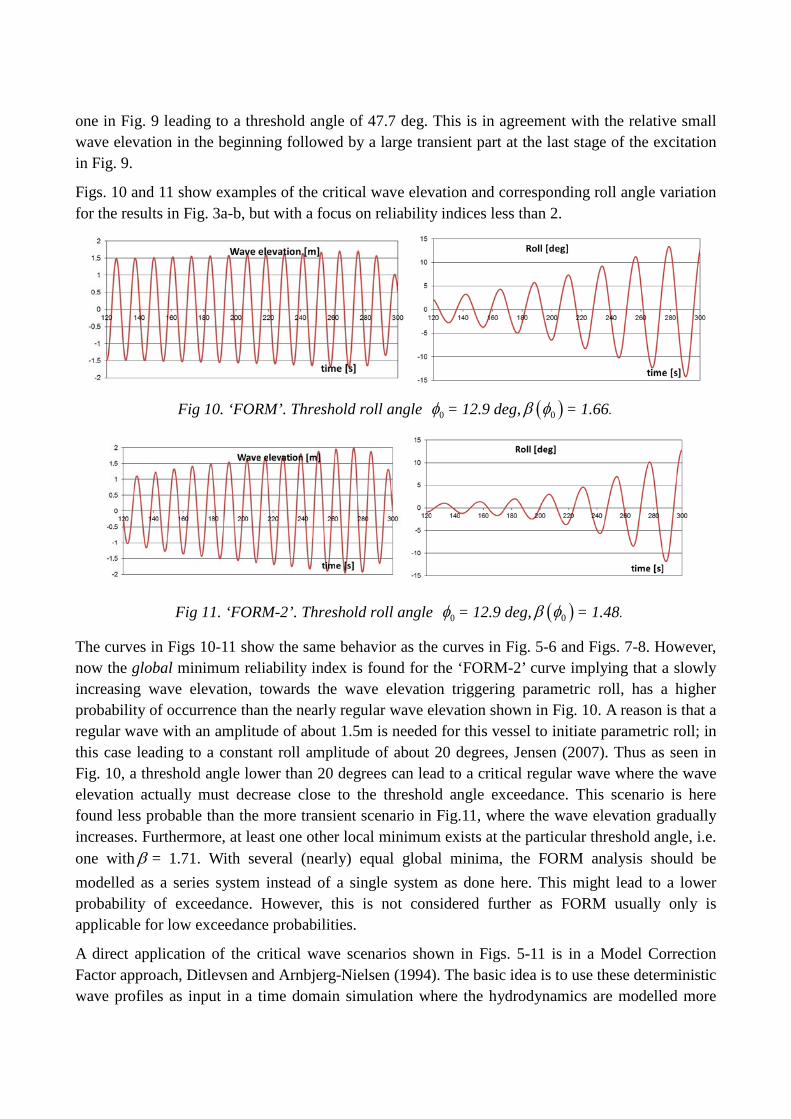
Figs. 10 and 11 show examples of the critical wave elevation and corresponding roll angle variation for the results in Fig. 3a-b, but with a focus on reliability indices less than 2.

Fig 10. ‘FORM’. Threshold roll angle 0φ = 12.9 deg, ( )0β φ = 1.66.

Fig 11. ‘FORM-2’. Threshold roll angle 0φ = 12.9 deg, ( )0β φ = 1.48.

The curves in Figs 10-11 show the same behavior as the curves in Fig. 5-6 and Figs. 7-8. However, now the global minimum reliability index is found for the ‘FORM-2’ curve implying that a slowly increasing wave elevation, towards the wave elevation triggering parametric roll, has a higher probability of occurrence than the nearly regular wave elevation shown in Fig. 10. A reason is that a regular wave with an amplitude of about 1.5m is needed for this vessel to initiate parametric roll; in this case leading to a constant roll amplitude of about 20 degrees, Jensen (2007). Thus as seen in Fig. 10, a threshold angle lower than 20 degrees can lead to a critical regular wave where the wave elevation actually must decrease close to the threshold angle exceedance. This scenario is here found less probable than the more transient scenario in Fig.11, where the wave elevation gradually increases. Furthermore, at least one other local minimum exists at the particular threshold angle, i.e. one with β = 1.71. With several (nearly) equal global minima, the FORM analysis should be modelled as a series system instead of a single system as done here. This might lead to a lower probability of exceedance. However, this is not considered further as FORM usually only is applicable for low exceedance probabilities.

A direct application of the critical wave scenarios shown in Figs. 5-11 is in a Model Correction Factor approach, Ditlevsen and Arnbjerg-Nielsen (1994). The basic idea is to use these deterministic wave profiles as input in a time domain simulation where the hydrodynamics are modelled more

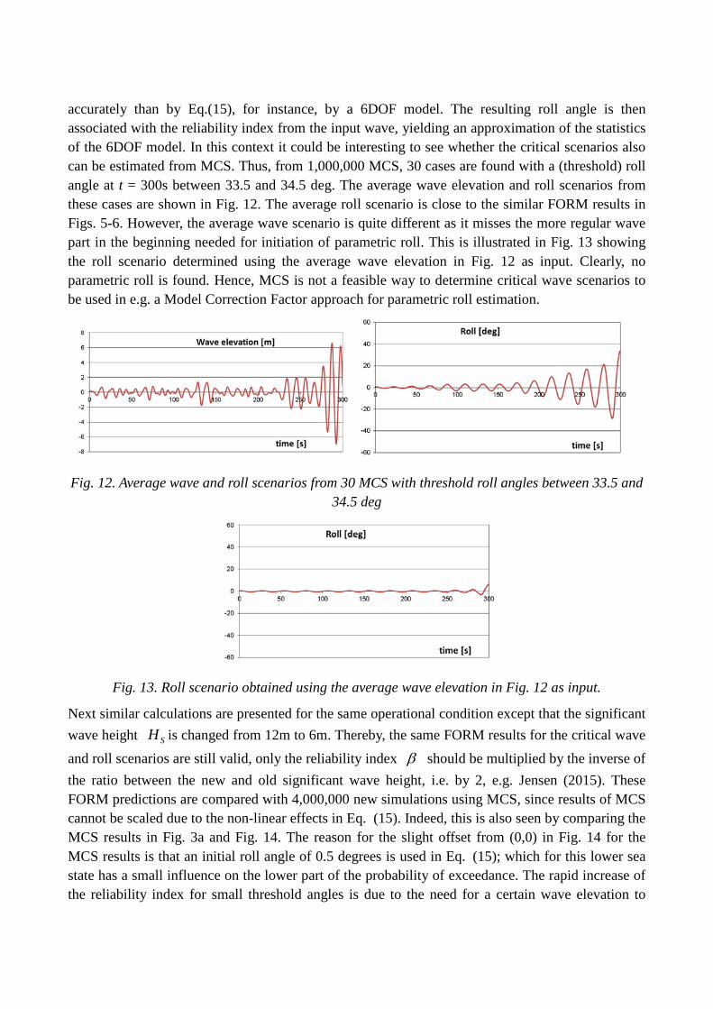
accurately than by Eq.(15), for instance, by a 6DOF model. The resulting roll angle is then associated with the reliability index from the input wave, yielding an approximation of the statistics of the 6DOF model. In this context it could be interesting to see whether the critical scenarios also can be estimated from MCS. Thus, from 1,000,000 MCS, 30 cases are found with a (threshold) roll angle at t = 300s between 33.5 and 34.5 deg. The average wave elevation and roll scenarios from these cases are shown in Fig. 12. The average roll scenario is close to the similar FORM results in Figs. 5-6. However, the average wave scenario is quite different as it misses the more regular wave part in the beginning needed for initiation of parametric roll. This is illustrated in Fig. 13 showing the roll scenario determined using the average wave elevation in Fig. 12 as input. Clearly, no parametric roll is found. Hence, MCS is not a feasible way to determine critical wave scenarios to be used in e.g. a Model Correction Factor approach for parametric roll estimation.

Fig. 12. Average wave and roll scenarios from 30 MCS with threshold roll angles between 33.5 and

34.5 deg

Fig. 13. Roll scenario obtained using the average wave elevation in Fig. 12 as input.

Next similar calculations are presented for the same operational condition except that the significant wave height SH is changed from 12m to 6m. Thereby, the same FORM results for the critical wave and roll scenarios are still valid, only the reliability index β should be multiplied by the inverse of the ratio between the new and old significant wave height, i.e. by 2, e.g. Jensen (2015). These FORM predictions are compared with 4,000,000 new simulations using MCS, since results of MCS cannot be scaled due to the non-linear effects in Eq. (15). Indeed, this is also seen by comparing the MCS results in Fig. 3a and Fig. 14. The reason for the slight offset from (0,0) in Fig. 14 for the MCS results is that an initial roll angle of 0.5 degrees is used in Eq. (15); which for this lower sea state has a small influence on the lower part of the probability of exceedance. The rapid increase of the reliability index for small threshold angles is due to the need for a certain wave elevation to

trigger parametric roll. The same asymptotic agreement between the MCS and FORM results for large values of the reliability index β is seen again.

If the probability of exceedance were to be requested for the whole range of threshold angles, the most effective procedure is to use MCS for the lower range and FORM for the higher range of β . If a Coefficient of Variation CoV of 10 percent on the probability of exceedance is required for the MCS, then the number of exceedance in the considered simulation should be around 100 and the total number of MCS roughly equal to 100 / ( 3)Φ − = 75,000, or about 2,000s in CPU time. An example of this interpolation is included in Fig. 14 where the FORM result for a threshold angle of 30 degrees is used as the upper point on this interpolation line. Approximately 80,000 calls (75,000 for the MCS and 5,000 for the single FORM result for 0φ = 30 degrees) are required to obtain this line; and, this number should be compared to the 4,000,000 simulations needed if the probability of exceedance is to be calculated up to a threshold angle equal to 30 degrees by MCS alone. Of course, other interpolation schemes can be applied between MCS and FORM results, e.g. Jensen (2015), but the important point is that it is interpolation and not extrapolation, as in the case using only MCS results.

Fig. 14. Reliability index β as function of threshold roll angle 0φ , derived from FORM and MCS.

SH = 6m.

CONCLUSION The paper suggests the use of the First Order Reliability method as a candidate for extreme value prediction of the maximum roll angle in parametric roll in random sea states. The method is fast and accurate for low probability of exceedance, and, combined with Monte Carlo simulation for high exceedance probabilities, fast and accurate extreme value predictions can be achieved. This can be useful, especially, in connection with operational guidelines and direct stability calculations for a specific operational profile for a ship.

REFERENCES 1. Bulian, G, Francescutto, A, Lugni, C, (2006). “Theoretical, numerical and experimental study on

the problem of ergodicity and ‘practical ergodicity’ with an application to parametric roll in longitudinal long crested irregular sea”, Ocean Engineering, Vol. 33, pp 1007–1043.

2. Choi, JH, Jensen, JJ, Nielsen, UD (2016), "A study on the uncertainty and sensitivity in numerical simulation of parametric roll", Proc 13th PRADS conference, September 4-8, 2016, Copenhagen, Denmark

3. Choi, JH, Jensen, JJ, Kristensen HO, Nielsen, UD, Ericksen, H (2017). “Intact stability analysis of dead ship conditions using FORM”, Submitted to J. Ship Research

4. Der Kiureghian, A (2000). “The geometry of Random Vibrations and Solutions by FORM and SORM”. Probabilistic Engineering Mechanics, Vol. 15, pp 81-90

5. Ditlevsen, O and Arnbjerg-Nielsen, T (1994). ”Model-Correction-Factor Method in Structural Reliability”. Journal of Engineering, Vol. 120, pp 1-10

6. France, WN, Levadou, M, Treakle, TW, Pauling, JR, Michel, RK, Moore, C (2003). “An investigation of head-sea parametric rolling and its infl uence on container lashing systems”. Mar Technology, Vol 40, pp 1–19

7. Grim, O (1961). ”Beitrag zu dem Problem der Sicherheit des Schiffes im Seegang”. Schiff und Hafen, Vol. 6, pp 490–497

8. Hasofer, AM and Lind, NC (1974). “Exact and invariant second .moment code format”. J. Eng Mech, Vol 100, pp111-121

9. IMO (2017),“Finalization of the Second Generation of Intact Stability Criteria -Danish Sample Ship Calculation 2016”, Sub-committee SDC, 4th session, Agenda item 5, SDC 4, http://www.skibstekniskselskab.dk/s/Sample-Calculation-Results-Intact-Stability.pdf

10. Jensen JJ and Capul J (2006). “Extreme Response Predictions for Jack-up Units in Second Order Stochastic Waves by FORM”. Probabilistic Engineering Mechanics, Vol 21, pp 330-337.

11. Jensen, JJ (2007). “Efficient estimation of extreme non-linear roll motions using the first-order reliability method (FORM)”. J. Marine Science and technology, Vol 12, No. 4, pp 191-202

12. Jensen JJ (2015). “Conditional stochastic processes applied to wave load predictions”. Weinblum Memorial Lecture, J. Ship Research, Vol 59, No. 1, pp. 1-10

13. Liu, P-L and Der Kiureghian, A (1991). ”Optimization algorithms for structural safety”. Structural Safety, Vol 9, pp 161-177

14. Naess, A and Gaidai, O (2009). “Estimation of Extreme Values from Sampled Time Series”. Structural Safety, Vol. 31, No. 4, pp 325-334

15. Nielsen, UD and Jensen, JJ (2011). ”A novel approach for navigational guidance of ships using onboard monitoring systems”, Ocean Engineering, Vol. 38, pp 444-455

16. Tompuri, M, Ruponen, P, Forss M, Lindroth, D (2015). “Application of the Second Generation Intact Stability Criteria in Initial Ship Design”, Transactions - Society of Naval Architects and Marine Engineers, Vol 122, pp 20-45

17. Vidic-Perunovic, J and Jensen, JJ (2009). “Parametric roll due to hull instantaneous volumetric changes and speed variations”, Ocean Engineering, Vol. 36, pp 891-899