Statistical SamplingStatistical Sampling

Summer 2003Summer 2003

15.063 Summer 200315.063 Summer 2003 22

STATISTICAL SAMPLING: An ExampleNEXNet is a relatively small but aggressive player in the telecommunications market in the mid-Atlantic region of the US. It is now considering a move into the Boston area.

NEXNet would like to estimate the average monthly phone bill in the communities of Weston, Wayland, and Sudbury, by conducting a phone survey. As an enticement for people to participate in the survey, NEXNet will offer discount coupons on certain products to survey participants.

• How many households should NEXNet plan to survey (successfully) in order to effectively estimate the average phone bill in these three communities?

• How should NEXNet analyze the survey results?

15.063 Summer 200315.063 Summer 2003 33

Outline• Random sample

• The sample mean and the sample standard deviation

• The distribution of the sample mean

• Confidence interval estimation.

• Sample size design

15.063 Summer 200315.063 Summer 2003 44

Random Sample

• Random Sample: a sample collected in such a way that everymember in the population is equally likely to be selected.

• Population: set of all units of interest

• Sample: a subset of the population

Our Goal: Make inferences, i.e., estimates, predictions, etc. about a population based on information from a sample.

In particular, we want to estimate the population mean µ , and the population standard deviation σ.

15.063 Summer 200315.063 Summer 2003 55

Examples of Statistical Sampling

• Marketing: Determine household income of consumers

• Manufacturing: Determine the fraction of defects in a batch

• Polling: Determine the proportion of population that favors a candidate

• Other Examples?

15.063 Summer 200315.063 Summer 2003 66

A Failed SurveyExample: 1936 U.S. presidential election, Alf Landon vs.

Franklin Roosevelt

• October 1936, Literary Digest conducted the largest poll in history: 10 million voter surveys mailed out. They had correctly predicted the winner since 1916 elections.

• The 2.4 million who completed the survey predicted that Landon would win by 57% to 43%.

• One month later, Roosevelt was re-elected with the largest majority in U.S. history.

• Results: Roosevelt 62% Landon 38%• The magazine went bankrupt soon after.

What went wrong?

15.063 Summer 200315.063 Summer 2003 77

Biased SamplingBiased SamplingNames gathered from mailing lists, subscriptions, and Names gathered from mailing lists, subscriptions, and telephone bookstelephone booksOnly 1 in 4 households had phones, biased toward the Only 1 in 4 households had phones, biased toward the wealthy (who supported Landon whereas the poor wealthy (who supported Landon whereas the poor supported Roosevelt)supported Roosevelt)Only 20% of surveys were returned (nonOnly 20% of surveys were returned (non--response bias)response bias)At the same time, George Gallup polled 3000 At the same time, George Gallup polled 3000 Literary Literary DigestDigest readers and correctly predicted the results. He readers and correctly predicted the results. He also polled 50,000 potential voters in a less biased also polled 50,000 potential voters in a less biased sample and predicted Roosevelt would get 56%.sample and predicted Roosevelt would get 56%.A larger A larger biasedbiased sample does not make a better sample! sample does not make a better sample!

15.063 Summer 200315.063 Summer 2003 88

A Financial ExampleA Financial Example

Imagine that you receive an email from an Imagine that you receive an email from an investment firm offering advice on winning investment firm offering advice on winning stocks, including a “free sample” stock pickstocks, including a “free sample” stock pickThe stock goes up that weekThe stock goes up that weekYou receive a second email naming a second You receive a second email naming a second stock that will go up in the next weekstock that will go up in the next weekIt goes upIt goes upA third email offers a third stock which goes upA third email offers a third stock which goes upThe fourth email solicits a newsletter The fourth email solicits a newsletter subscription. subscription. Would you subscribe?Would you subscribe?

15.063 Summer 200315.063 Summer 2003 99

Biased Sampling AgainBiased Sampling AgainIt is natural to assume that the stocks in the It is natural to assume that the stocks in the emails are randomly chosen from a list of “buy” emails are randomly chosen from a list of “buy” recommendationsrecommendationsBut suppose instead that different potential But suppose instead that different potential customers got customers got differentdifferent recommendations recommendations selected at selected at randomrandom, and the recipients of “failed , and the recipients of “failed predictions” were then predictions” were then dropped dropped from further from further noticesnoticesIf stock predictions are random (50% chance the If stock predictions are random (50% chance the stock will go up), then the odds of getting three stock will go up), then the odds of getting three hits in a row are 1 in 8hits in a row are 1 in 8That may be enough to attract lots of business!That may be enough to attract lots of business!

15.063 Summer 200315.063 Summer 2003 1010

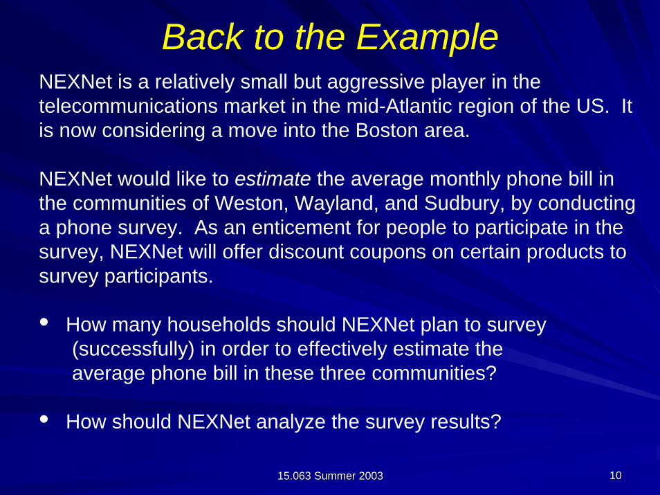
Back to the ExampleNEXNet is a relatively small but aggressive player in the telecommunications market in the mid-Atlantic region of the US. It is now considering a move into the Boston area.

NEXNet would like to estimate the average monthly phone bill in the communities of Weston, Wayland, and Sudbury, by conducting a phone survey. As an enticement for people to participate in the survey, NEXNet will offer discount coupons on certain products to survey participants.

• How many households should NEXNet plan to survey (successfully) in order to effectively estimate the average phone bill in these three communities?

• How should NEXNet analyze the survey results?

15.063 Summer 200315.063 Summer 2003 1111

Sample Histogram of May Phone Bills (sample size n = 70)

Observation May Observation May Observation May Number Phone Bill Number Phone Bill Number Phone Bill

1 $95.67 25 $79.32 49 $90.022 $82.69 26 $89.12 50 $61.063 $75.27 27 $63.12 51 $51.004 $145.20 28 $145.62 52 $97.715 $155.20 29 $37.53 53 $95.446 $80.53 30 $97.06 54 $31.897 $80.81 31 $86.33 55 $82.358 $60.93 32 $69.83 56 $60.209 $86.67 33 $77.26 57 $92.2810 $56.31 34 $64.99 58 $120.8911 $151.27 35 $57.78 59 $35.0912 $96.93 36 $61.82 60 $69.5313 $65.60 37 $74.07 61 $49.8514 $53.43 38 $141.17 62 $42.3315 $63.03 39 $48.57 63 $50.0916 $139.45 40 $76.77 64 $62.6917 $58.51 41 $78.78 65 $58.6918 $81.22 42 $62.20 66 $127.8219 $98.14 43 $80.78 67 $62.4720 $79.75 44 $84.51 68 $79.2521 $72.74 45 $93.38 69 $76.5322 $75.99 46 $139.23 70 $74.1323 $80.35 47 $48.0624 $49.42 48 $44.51

15.063 Summer 200315.063 Summer 2003 1212

THE HISTOGRAM

HistogramHistogram

00

4.04.0

4040 6060 8080 100100 120120 140140 MoreMoreMonthly Phone Bill ($)Monthly Phone Bill ($)

Freq

uenc

y (%

)Fr

eque

ncy

(%)

10.010.0

8.08.0

5050 7070 9090 110110 130130 150150

15.063 Summer 200315.063 Summer 2003 1313

The ProblemThe ProblemWe will discuss how to determine the We will discuss how to determine the appropriate sample size n later.appropriate sample size n later.

Our current problem is:Our current problem is:

Based on these n anticipated sample values Based on these n anticipated sample values XX11, X, X22, . . . , X, . . . , Xnn , we want to make , we want to make inferencesinferencesabout the entire population.about the entire population.

Why? Because Why? Because NEXNetNEXNet has been profitable has been profitable in communities with mean bills > $75, and no in communities with mean bills > $75, and no more than 15% households < $45 and at least more than 15% households < $45 and at least 30% bills between $60 and $10030% bills between $60 and $100

15.063 Summer 200315.063 Summer 2003 1414

Estimates of the Population Mean

Sample Mean: sum of all the sample observations divided by the number of observations

X = X1 + X2 + . . . + Xnn

Sample Median: the value that one-half the observations are below (50th percentile)

15.063 Summer 200315.063 Summer 2003 1515

HistogramHistogram

00

4.04.0

4040 6060 8080 100100 120120 140140 MoreMoreMonthly Phone Bill ($)Monthly Phone Bill ($)

Freq

uenc

y (%

)Fr

eque

ncy

(%)

10.010.0

8.08.0

5050 7070 9090 110110 130130 150150

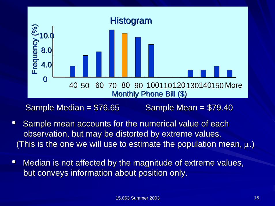
Sample Median = $76.65 Sample Mean = $79.40 Sample Median = $76.65 Sample Mean = $79.40

•• Sample mean accounts for the numerical value of eachSample mean accounts for the numerical value of eachobservation, but may be distorted by extreme values. observation, but may be distorted by extreme values.

(This is the one we will use to estimate the population mean, (This is the one we will use to estimate the population mean, µµ.).)

•• Median is not affected by the magnitude of extreme values, Median is not affected by the magnitude of extreme values, but conveys information about position only.but conveys information about position only.

15.063 Summer 200315.063 Summer 2003 1616

Estimate of the Population Standard Deviation

• The sample variance S2 is an “unbiased estimator’’ of the population variance, i.e., E [S2] = Var[X] = σ 2.

• The sample standard deviation s is:

• We will use S to estimate the population standard deviation σ.

S = ( )Xi -2XΣi=1

n

n - 1

• Question: Why n - 1, and not n (as in the formula for calculating the population SD)?

• Answer: It gives a better (slightly larger) estimate. See: http://mathcentral.uregina.ca/QQ/database/QQ.09.99/freeman2.html

• When n is large, the difference is negligible.

15.063 Summer 200315.063 Summer 2003 1717

Example ContinuedNEXNet arranged to have 70 randomly selected households successfully surveyed, as shown in the table. It found that the observed sample mean of the monthly phone bill was $79.40, and the observed sample standard deviation was $28.79.

• How would you characterize the shape of the distribution?Answer: It is not Normally distributed (some “outliers”).

• What is your estimate of the actual mean µ ?

x = $79.40

• What is your estimate of the actual standard deviation σ ?

s = $28.79

15.063 Summer 200315.063 Summer 2003 1818

Clarify the Sampling ProcedureBefore we collect the sample,

• X1, X2, . . . , Xn are the values that will arise from the sample

• X1, X2, . . . , Xn are random variables, i. i. d.• As a result, we have for each Xi: E[Xi] = µ, Var[Xi] = σ 2.

• is the sample standard deviation also a r.v. ?

• ; The sample mean is a r.v. why?X = X1 + X2 + . . . + Xnn

S = ( )Xi -2XΣi=1

n

n - 1

Since both the sample mean and the sample standard deviation are r.v.’s, we will get different results from different samples!

15.063 Summer 200315.063 Summer 2003 1919

Estimating the Population Estimating the Population Mean Using the Sample MeanMean Using the Sample Mean

Population

(parameter)µ

Sample

x(statistic )

µ estimate tox Calculate

Select arandom sample

Process ofInferential Statistics

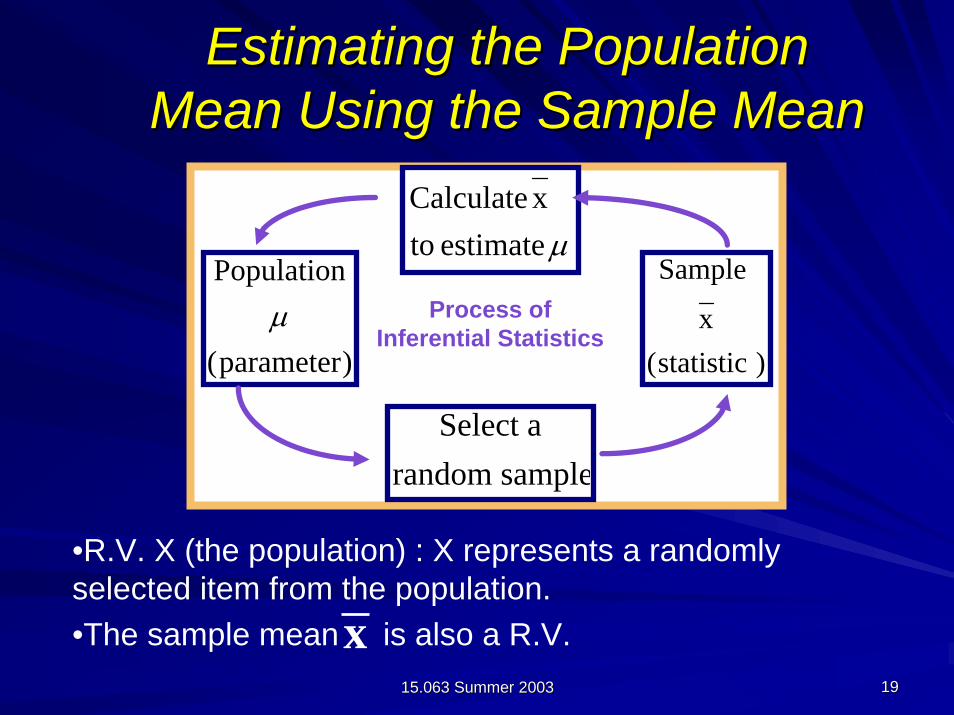
•R.V. X (the population) : X represents a randomly selected item from the population.•The sample mean is also a R.V.x

15.063 Summer 200315.063 Summer 2003 2020

What is the variability of the mean?What is the variability of the mean?

Random variable X is defined as the average of n Random variable X is defined as the average of n independent and identically distributed random independent and identically distributed random variables, Xvariables, X11, X, X22, …, X, …, Xnn; with mean, ; with mean, µ,µ, and Sd, and Sd, σσ. . Then, for Then, for large enough nlarge enough n (typically (typically nn≥≥3030), X is ), X is approximately Normally distributedapproximately Normally distributed with with parameters: parameters: µµxx = = µ µ and and σσxx = = σ/ σ/ nn

This result holds regardless of the shape of the X This result holds regardless of the shape of the X distribution (i.e. the Xs don’t have to be normally distribution (i.e. the Xs don’t have to be normally distributed!)distributed!)And we can continue to estimate σ with s

15.063 Summer 200315.063 Summer 2003 2121

Estimating the population mean using an Interval Estimating the population mean using an Interval

X Zn

or

X Zn

X Zn

±

− ≤ ≤ +

σ

σ µ σ

( )

S

XXSS

n2

2

2

1

=

−=∑ −

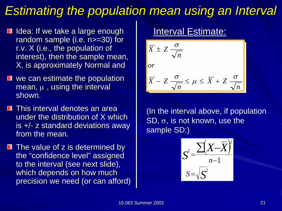
Idea: If we take a Idea: If we take a large enoughlarge enoughrandom sample (i.e. random sample (i.e. n>=30n>=30) for ) for r.v. X (i.e., the population of r.v. X (i.e., the population of interest), then the sample mean, interest), then the sample mean, X, is X, is approximately Normalapproximately Normal andand

we can we can estimate estimate the population the population meanmean, , µµ ,, using the interval using the interval shown.shown.

This interval denotes an area This interval denotes an area under the distribution of X which under the distribution of X which is +/is +/-- z standard deviations away z standard deviations away from the mean. from the mean.

The value of z is determined by The value of z is determined by the “confidence level” assigned the “confidence level” assigned to the interval (see next slide), to the interval (see next slide), which depends on how much which depends on how much precision we need (or can afford)precision we need (or can afford)

Interval Estimate:

(In the interval above, if population SD, σ, is not known, use the sample SD:)

15.063 Summer 200315.063 Summer 2003 2222

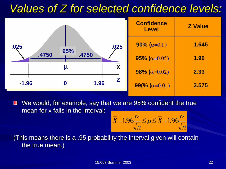
Values of Z for selected confidence levels:Values of Z for selected confidence levels:

We would, for example, say that we are 95% confident the true We would, for example, say that we are 95% confident the true mean for x falls in the interval:mean for x falls in the interval:

(This means there is a .95 probability the interval given will c(This means there is a .95 probability the interval given will contain ontain the true mean.)the true mean.)

µ

.4750 .4750

X

95%.025.025

Z1.96-1.96 0

90% (α=0.1)

95% (α=0.05)

98% (α=0.02)

99(% (α=0.01)

Confidence Level Z Value

1.645

1.96

2.33

2.575

nX

nX σµσ 96.196.1 +≤≤−

15.063 Summer 200315.063 Summer 2003 2323

Example ContinuedCalculate a 95% confidence interval for Nextel’s mean monthly phone bill. monthly phone bill. Formula:Formula: Data:Data:

1.96 * 28.79 / sqrt(70) = 6.74.

X Zn

or

X Zn

X Zn

±

− ≤ ≤ +

σ

σ µ σ

= $79.40; s = $28.79; n=70;

For CL 95% z=1.96

x

• We are 95% confident that the true mean µ is within 6.74of the sample mean of 79.40 or [79.40 - 6.74, 79.40 + 6.74].

• The interval [72.66, 86.14] is called a 95% confidence interval (C.I.) for the population mean.

15.063 Summer 200315.063 Summer 2003 2424

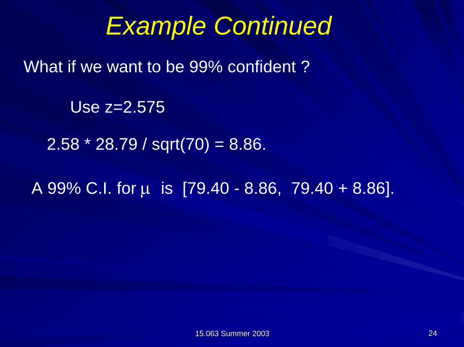
Example ContinuedWhat if we want to be 99% confident ?

Use z=2.575

2.58 * 28.79 / sqrt(70) = 8.86.

A 99% C.I. for µ is [79.40 - 8.86, 79.40 + 8.86].

15.063 Summer 200315.063 Summer 2003 2525

Interpreting confidence intervalsInterpreting confidence intervalsInterpreting confidence intervals

......

True population meanTrue population mean

In a usual application, we In a usual application, we only sample once and only sample once and report a single confidence report a single confidence level, for example,level, for example, 95%.95%.

If we repeated this sampling If we repeated this sampling procedure 100 times, our procedure 100 times, our ((randomrandom) intervals will capture ) intervals will capture the true population mean, on the true population mean, on average, 95 times out of the 100 average, 95 times out of the 100 times.times.Sample 100Sample 100

Sample 18Sample 18

Sample 3Sample 3

Sample 1Sample 1

Sample 2Sample 2

......

15.063 Summer 200315.063 Summer 2003 2626

An ExampleAn ExampleEach person take a coin and flip it ten times; count the Each person take a coin and flip it ten times; count the number of heads and divide by tennumber of heads and divide by tenThis is your This is your observedobserved value of the proportion of headsvalue of the proportion of headsCalculate the Calculate the observedobserved standard deviation s (heads=1, standard deviation s (heads=1, tails=0, use the formula for s)tails=0, use the formula for s)Calculate a 90% confidence interval for the proportion of Calculate a 90% confidence interval for the proportion of heads from heads from youryour individual data (z=1.65)individual data (z=1.65)We know the true (theoretical) mean is 5. Is the true We know the true (theoretical) mean is 5. Is the true mean outside your 90% confidence interval?mean outside your 90% confidence interval?Note that the true standard deviation is Note that the true standard deviation is sqrtsqrt (n*p*[1(n*p*[1--p]) = p]) = sqrtsqrt (2.5) = 1.58, so the 90% confidence interval is 2.39 (2.5) = 1.58, so the 90% confidence interval is 2.39 to 7.61. to 7.61.

15.063 Summer 200315.063 Summer 2003 2727

Interpreting confidence intervalsInterpreting confidence intervalsInterpreting confidence intervals

......

True population mean = .5True population mean = .5

In a usual application, we In a usual application, we only sample once and only sample once and report a single confidence report a single confidence level, in our case,level, in our case, 90%.90%.

When we repeat this sampling When we repeat this sampling procedure 50 times, our procedure 50 times, our ((randomrandom) intervals will capture ) intervals will capture the true population mean, on the true population mean, on average, 45 times out of 50.average, 45 times out of 50.

Sample 50Sample 50

Sample 18Sample 18

Sample 3Sample 3

Sample 1Sample 1

Sample 2Sample 2

......

15.063 Summer 200315.063 Summer 2003 2828

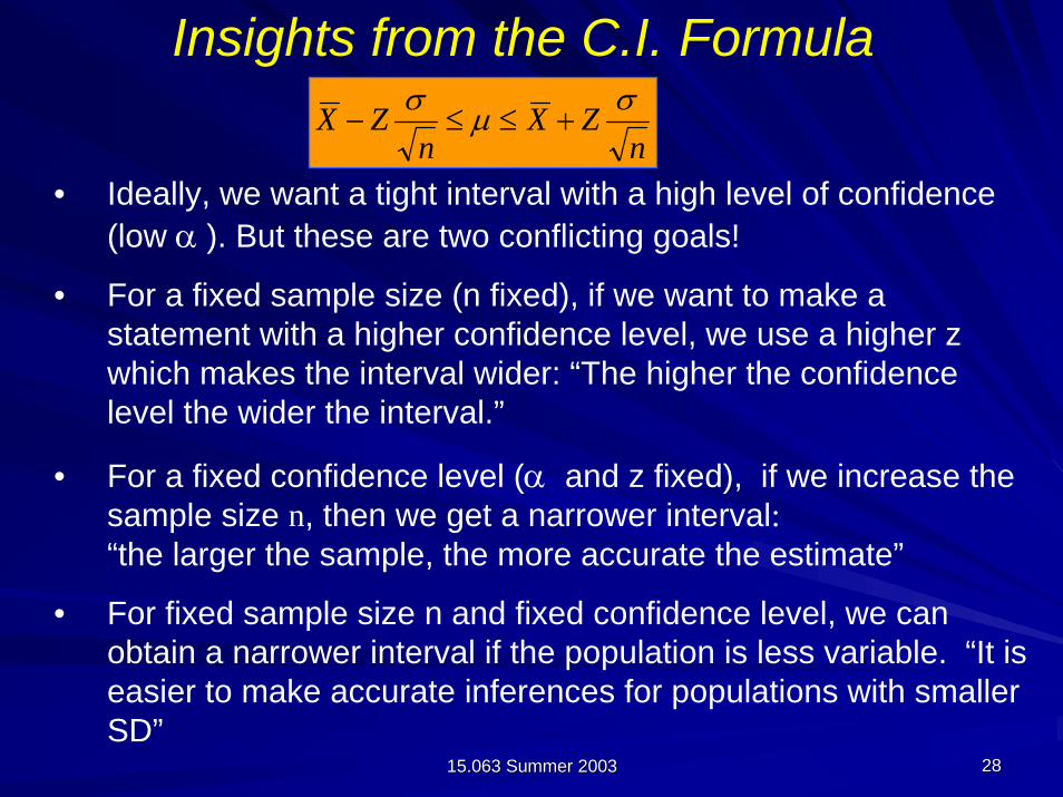
Insights from the C.I. Formula

• Ideally, we want a tight interval with a high level of confidence(low α ). But these are two conflicting goals!

• For a fixed sample size (n fixed), if we want to make a statement with a higher confidence level, we use a higher z which makes the interval wider: “The higher the confidence level the wider the interval.”

• For a fixed confidence level (α and z fixed), if we increase the sample size n, then we get a narrower interval: “the larger the sample, the more accurate the estimate”

• For fixed sample size n and fixed confidence level, we can obtain a narrower interval if the population is less variable. “It is easier to make accurate inferences for populations with smaller SD”

nZX

nZX σµσ

+≤≤−

15.063 Summer 200315.063 Summer 2003 2929

Experimental Design: How large a sample do we need?

• Usually the goal is to reach an estimate of the mean which is within a certain tolerance value L from the population mean:

• From we see that:

• For a given z associated with a given CL, α, and given population SD, σ ,(or sample SD s). We can solve for the required sample size n (we always round up!)

nZL σ

=

LXLX +≤≤− µ

nZX

nZX σµσ

+≤≤−

z2 s2

L2n =

15.063 Summer 200315.063 Summer 2003 3030

Estimating Sample SizeEstimating Sample Size

Suppose we needed to be 95% sure of being within $4 Suppose we needed to be 95% sure of being within $4 of the true population mean, what sample do we need?of the true population mean, what sample do we need?

L = 4, z = 1.96, and s = 28.79L = 4, z = 1.96, and s = 28.79n = zn = z22ss22/L/L2 2 = 1.96*1.96*28.79*28.79/(4*4)= 1.96*1.96*28.79*28.79/(4*4)N = 199.01N = 199.01As a rule of thumb, n should always be rounded up to As a rule of thumb, n should always be rounded up to the nearest number, so we need a sample of 200

For confidence = 90 or α= 10, z = 1.645For confidence = 95 or α= 5, z = 1.96For confidence = 99 or α = 1, z = 2.575

the nearest number, so we need a sample of 200

15.063 Summer 200315.063 Summer 2003 3131

Another example: How large a sample do we need?

A marketing research firm wants to conduct a survey to estimate the average amount spent by each person visiting a popular resort. The survey planners would like to estimate the mean amount within (±) $120, with 95% confidence. (For the moment, assume that the population standard deviation of spending at the resort is σ = $500.)

What is the sample size (n) you would need?

1.962 * 5002

1202 = 66.69 (use n=67)n =

If we don’t know σ , we first estimate it with s in a pilot run.

15.063 Summer 200315.063 Summer 2003 3232

Summary and Look AheadSummary and Look Ahead

Statistical sampling is about the value of Statistical sampling is about the value of information: how much information is needed, at information: how much information is needed, at what cost?what cost?Confidence intervals help us understand our Confidence intervals help us understand our level of uncertainty, which we can decide to level of uncertainty, which we can decide to reduce by collecting more datareduce by collecting more dataNext session we will talk about simulation, which Next session we will talk about simulation, which helps us introduce uncertainty explicitly into our helps us introduce uncertainty explicitly into our decision treesdecision trees