Network Tomography:Recent DevelopmentsRui Castro, Mark Coates, Gang Liang, Robert Nowak and Bin Yu
Abstract. Today’s Internet is a massive, distributed network which contin-ues to explode in size as e-commerce and related activities grow. The hetero-geneous and largely unregulated structure of the Internet renders tasks suchas dynamic routing, optimized service provision, service level verificationand detection of anomalous/malicious behavior extremely challenging. Theproblem is compounded by the fact that one cannot rely on the cooperationof individual servers and routers to aid in the collection of network trafficmeasurements vital for these tasks. In many ways, network monitoring andinference problems bear a strong resemblance to other “inverse problems”in which key aspects of a system are not directly observable. Familiar sig-nal processing or statistical problems such as tomographic image reconstruc-tion and phylogenetic tree identification have interesting connections to thosearising in networking. This article introduces network tomography, a newfield which we believe will benefit greatly from the wealth of statistical the-ory and algorithms. It focuses especially on recent developments in the fieldincluding the application of pseudo-likelihood methods and tree estimationformulations.
Key words and phrases: Network tomography, pseudo-likelihood, topologyidentification, tree estimation.
1. INTRODUCTION
No network is an island, entire of itself; every net-work is a piece of an internetwork, a part of the main(with apologies to John Donne, Devotions XVII. Med-itation). Although administrators of small-scale net-
Rui Castro is a Ph.D. student, DSP Group, Departmentof Electrical and Computer Engineering, Rice Uni-versity, Houston, Texas 77005, USA (e-mail: [email protected]). Mark Coates is Assistant Professor, Depart-ment of Electrical and Computer Engineering, McGillUniversity, Montreal, Quebec, Canada H3A 2A7(e-mail: [email protected]). Gang Liang is a Ph.D.student, Department of Statistics, University of Cal-ifornia, Berkeley, California 94720, USA (e-mail:[email protected]). Robert Nowak is AssociateProfessor, Department of Electrical and Computer En-gineering, University of Wisconsin, Madison, Wiscon-sin 53706, USA. Bin Yu is Professor, Department ofStatistics, University of California, Berkeley, Califor-nia 94720, USA.
works can monitor local traffic conditions and iden-tify congestion points and performance bottlenecks,very few networks are completely isolated. The user-perceived performance of a network thus dependsheavily on the performance of an internetwork, andmonitoring this internetwork is extremely challenging.Diverse subnetwork ownership and the decentralized,heterogeneous and unregulated nature of the extendedinternetwork combine to render a coordinated mea-surement framework infeasible. There is no real in-centive for individual servers and routers to collect andfreely distribute vital network statistics such as trafficrates, link delays and dropped packet rates. Collectingall pertinent network statistics imposes an impractica-ble overhead expense in terms of added computational,communication, hardware and maintenance require-ments. Even when data collection is possible, networkowners generally regard the statistics as highly confi-dential. Finally, the task of relaying measurements tothe locations where decisions are made consumes ex-orbitant bandwidth and presents scheduling and coor-dination nightmares.
499
500 R. CASTRO, M. COATES, G. LIANG, R. NOWAK AND B. YU
Despite this state of affairs, accurate, timely andlocalized estimates of network performance charac-teristics are vital ingredients in efficient network op-eration. With performance estimates in hand, moresophisticated and ambitious traffic control protocolsand dynamic routing algorithms can be designed.Quality-of-service guarantees can be provided if avail-able bandwidth can be gauged; the resulting service-level agreements can be verified. Detecting anomalousor malicious behavior becomes a more achievable task.
Usually we cannot directly measure the aspects ofthe system that we need to make informed decisions.However, we can frequently make useful measure-ments that do not require special cooperation from in-ternal network devices and do not inordinately impactnetwork load. Sophisticated methods of active networkprobing or passive traffic monitoring can generatenetwork statistics that indirectly relate to the perfor-mance measures we require. Subsequently, we canapply inference techniques, derived in the context ofother statistical inverse problems, to extract the hiddeninformation of interest.
This article surveys the field of inferential net-work monitoring or network tomography, highlight-ing challenges and open problems, and identifying keyissues that must be addressed. It builds upon the sig-nal processing survey paper by Coates, Hero, Nowakand Yu (2002b) and focuses on recent developmentsin the field. The task of inferential network monitor-ing demands the estimation of a potentially very largenumber of spatially distributed parameters. To suc-cessfully address such large-scale estimation tasks,researchers adopt models that are as simple as possi-ble but do not introduce significant estimation error.Such models are not suitable for intricate analysis ofnetwork queuing dynamics and fine time-scale traf-fic behavior, but they are often sufficient for infer-ence of performance characteristics. The approachshifts the focus from detailed queuing analysis andtraffic modeling (Kelly, Zachary and Ziedins, 1996;Chao, Miyazawa and Pinedo, 1999) to careful designof measurement techniques and large-scale inferencestrategies.
Measurement may be passive (monitoring trafficflows and sampling extant traffic) or active (gener-ating probe traffic). In either case, statistical modelsshould be developed for the measurement process, andthe temporal and spatial dependence of measurementsshould be assessed. These are active areas of researchin network tomography that we do not directly address
in this paper (see Section 5 for a summary of future di-rections). If existing traffic is being used to sample thestate of the network, care must be taken that the tem-poral and spatial structure of the traffic process doesnot bias the sample. If probes are used, then the actof measurement must not significantly distort the net-work state. Design of the measurement methodologymust take into account the limitations of the network.As an example, the clock synchronization required formeasurement of one-way packet delay is extremely dif-ficult.
Once measurement has been accomplished, statis-tical inference techniques can be applied to determineperformance attributes that cannot be directly observed.When attempting to infer a network performance mea-sure, measurement methodology and statistical infer-ence strategy must be considered jointly. In work thusfar in this area, a broad array of statistical techniqueshas been employed: complexity-reducing hierarchicalstatistical models; moment- and likelihood-based esti-mation; expectation–maximization and Markov chainMonte Carlo algorithms. However, the field is still inthe embryonic phase, and we believe that it can benefitgreatly from the wealth of extant statistical theory andalgorithms.
In this article, we focus exclusively on inferentialnetwork monitoring techniques that require minimalcooperation from network elements that cannot bedirectly controlled. Numerous tools exist for activeand passive measurement of networks (see http://www.caida.org/tools for a survey). The tools measure andreport internetwork attributes such as bandwidth, con-nectivity and delay, but they do not attempt to usethe recorded information to infer any performance at-tributes that have not been directly measured. The ma-jority of the tools depend on accurate reporting by allnetwork elements traversed during measurement.
The article commences by reviewing the area ofinternetwork inference and tomography, and providesa simple, generalized formulation of the network to-mography problem. In Section 3 we describe a pseudo-likelihood approach to network tomography that ad-dresses some of the scalability limitations of existingtechniques. We consider the problem of determiningthe connectivity structure or topology of a network andrelate this task to the problem of hierarchical cluster-ing. We introduce new likelihood-based hierarchicalclustering methods and results for identifying networktopology. Finally, we identify open problems and pro-vide our vision of future challenges.
NETWORK TOMOGRAPHY 501
2. NETWORK TOMOGRAPHY
2.1 Network Tomography Basics
Large-scale network inference problems can be clas-sified according to the type of data acquisition andthe performance parameters of interest. To discussthese distinctions, we require some basic definitions.Consider the network depicted in Figure 1. Each noderepresents a computer terminal, router or subnetwork(consisting of multiple computers/routers). A connec-tion between two nodes is called a path. Each path con-sists of one or more links—direct connections with nointermediate nodes. The links may be unidirectional orbidirectional, depending on the level of abstraction andthe problem context. Each link can represent a chain ofphysical links connected by intermediate routers. Mes-sages are transmitted by sending packets of bits from asource node to a destination node along a path whichgenerally passes through several other nodes.
Broadly speaking, large-scale network inference in-volves estimating network performance parametersbased on traffic measurements at a limited subsetof the nodes. Vardi (1996) was one of the first re-searchers to rigorously study this sort of problemand he coined the term network tomography due tothe similarity between network inference and med-ical tomography. Two forms of network tomographyhave been addressed in the recent literature: (1) link-level parameter estimation based on end-to-end, path-level traffic measurements (http://gaia.cs.umass.edu/minc; Cáceres, Duffield, Horowitz and Towsley, 1999;Ratnasamy and McCanne, 1999; Coates and Nowak,2000; Harfoush, Bestavros and Byers, 2000; Duffield,Lo Presti, Paxson and Towsley, 2001; Shih and Hero,2001; Ziotopolous, Hero and Wasserman, 2001; LoPresti, Duffield, Horowitz and Towsley, 2002; Tsang,Coates and Nowak, 2003) and (2) sender–receiverpath-level traffic intensity estimation based on link-level traffic measurements (Vanderbei and Iannone,
FIG. 1. An arbitrary virtual multicast tree with four receivers.
1994; Vardi, 1996; Tebaldi and West, 1998; Cao,Davis, Vander Wiel and Yu, 2000a; Cao, Vander Wiel,Yu and Zhu, 2000b; Liang and Yu, 2003b).
In link-level parameter estimation, the traffic mea-surements typically consist of counts of packets trans-mitted and/or received between source and destinationnodes or time delays between packet transmissions andreceptions. The goal is to estimate the loss rate or thequeuing delay on each link. The measured time delaysare due to both propagation delays and router process-ing delays along the path. The path delay is the sum ofthe delays on the links that comprise the path; the linkdelay comprises both the propagation delay on that linkand the queuing delay at the routers that lie along thatlink. A packet is dropped if it does not successfullyreach the input buffer of the destination node. Linkdelays and occurrences of dropped packets are inher-ently random. Random link delays can be caused byrouter output buffer delays, router packet servicing de-lays and propagation delay variability. Dropped pack-ets on a link are usually due to overload of the finiteoutput buffer of one of the routers encountered whentraversing the link, but may also be caused by equip-ment downtime due to maintenance or power failures.Random link delays and packet losses become particu-larly substantial when there is a large amount of cross-traffic competing for service by routers along a path.
In path-level traffic intensity estimation, the measu-rements consist of counts of packets that pass throughnodes in the network. In privately owned networks, thecollection of such measurements is relatively straight-forward. Based on these measurements, the goal is toestimate how much traffic originated from a specifiednode and was destined for a specified receiver. Thecombination of the traffic intensities of all these origin–destination pairs forms the origin–destination trafficmatrix. In this problem not only are the node-levelmeasurements inherently random, but the parameterto be estimated (the origin–destination traffic matrix)must itself be treated not as a fixed parameter, but asa random vector. Randomness arises from the trafficgeneration itself, rather than perturbations or measure-ment noise.
The inherent randomness in both link-level and path-level measurements motivates the adoption of statis-tical methodologies for large-scale network inferenceand tomography. Many network tomography problemscan be roughly approximated by the (not necessarilyGaussian) linear model
Yt = AXt + ε,(1)
502 R. CASTRO, M. COATES, G. LIANG, R. NOWAK AND B. YU
where Yt is a vector of measurements (e.g., packetcounts or end-to-end delays) recorded at a given time t
at a number of different measurement sites, A is a rout-ing matrix, ε is a noise vector and Xt is a vector oftime-dependent packet parameters (e.g., mean delays,logarithms of packet transmission probabilities over alink or the random origin–destination traffic vector). Insome cases the vector Xt is a random vector with an un-derlying parameterized distribution f (Xt |θ t ) (see theexample in Section 3.1), and it is the parameters θ t
that interest us. Typically, but not always, A is a bi-nary matrix (the i, j th element is equal to 1 or 0) thatcaptures the topology of the network. In this paper, weconsider the problems of using the observations Yt toestimate θ t (see Section 3.1), Xt (see Section 3.2) or A(see Section 4).
What sets the large-scale network inference prob-lem (1) apart from other network inference problems isthe potentially very large dimension of A which canrange from a half a dozen rows and columns for afew packet parameters and a few measurement sitesin a small local area network, to thousands or tens ofthousands of rows and columns for a moderate num-ber of parameters and measurements sites in the In-ternet. The associated high-dimensional problems ofestimating Xt are specific examples of inverse prob-lems. Inverse problems have a very extensive literature(O’Sullivan, 1986). Solution methods for such inverseproblems depend on the nature of the noise ε and the Amatrix, and typically require iterative algorithms sincethey cannot be solved directly. In general, A is notfull rank, so that identifiability concerns arise. Eitherone must be content to resolve only linear combina-tions of the parameters or one must employ statisticalmeans to introduce regularization and induce identi-fiability. Both tactics are utilized in the examples inlater sections of the article. In most of the large-scaleInternet inference and tomography problems studiedto date, the components of the noise vector ε areassumed to be approximately independent Gaussian,Poisson, binomial or multinomial distributed. Whenthe noise is Gaussian distributed with covariance inde-pendent of AXt , methods such as recursive linear leastsquares can be implemented using conjugate gradi-ent, Gauss–Seidel and other iterative equation solvers.When the noise is modeled as Poisson, binomial ormultinomial distributed, more sophisticated statisticalmethods, such as reweighted nonlinear least squares,maximum likelihood via expectation–maximization(EM) and maximum a posteriori via Markov chainMonte Carlo (MCMC) algorithms, become necessary.
3. PSEUDO-LIKELIHOOD APPROACHES
In developing methods to perform network tomog-raphy, there is a trade-off between statistical effi-ciency (accuracy) and computational overhead. In thepast, researchers have addressed the extreme compu-tational burden posed by some of the tomographicproblems, developing suboptimal but lightweight al-gorithms, including a fast recursive algorithm for linkdelay distribution inference in a multicast framework(Lo Presti et al., 2002) and a method-of-moments ap-proach for origin–destination matrix inference (Vardi,1996). More accurate but computationally burden-some approaches have also been explored, includ-ing maximum-likelihood methods (Coates and Nowak,2000; Tsang, Coates and Nowak, 2003; Cao et al.,2002a), but in general they are too intensive compu-tationally for any network of reasonable scale.
More recently, we proposed a unified pseudo-likeli-hood approach (Liang and Yu, 2003a, b) that easesthe computational burden but maintains good statis-tical efficiency. The idea of modifying likelihood isnot new, and many modified likelihood models havebeen proposed, for example, pseudo-likelihood forMarkov random fields by Besag (1974, 1975), par-tial likelihood for hazards regression by Cox (1975)and quasi-maximum likelihood for finance modelsby White (1994). In this section, we decribe thepseudo-likelihood approach. We explore two concreteexamples: (1) internal link delay distribution infer-ence through multicast end-to-end measurements and(2) origin–destination (OD) matrix inference throughlink traffic counts (the OD matrix specifies the volumeof traffic between a source and a destination).
The network tomography model we consider in thissection is a special case of (1), in which the errorterm ε is omitted for further simplification. Hence themodel can be rewritten as
Y = AX,(2)
where X = (X1, . . . ,XJ )′ is a J -dimensional vec-tor of network dynamic parameters (e.g., link de-lay, traffic flow counts at a particular time interval),Y = (Y1, . . . , YI )
′ is an I -dimensional vector of mea-surements and A is an I × J routing matrix.
As mentioned before, A is not full rank in a generalnetwork tomography scenario, where typically I � J ;hence, constraints have to be introduced to ensure theidentifiability of the model. A key assumption is that allcomponents of X are independent of each other. Suchan assumption does not hold strictly in a real network
NETWORK TOMOGRAPHY 503
due to the temporal and spatial correlations betweennetwork traffic, but it is a good first-step approxima-tion. Furthermore, we assume that
Xj ∼ fj (θj ), j = 1, . . . , J,(3)
where fj is a density function and θj is its para-meter. Then the parameter of the whole model isθ = (θ1, . . . , θJ ). In our first network tomography ex-ample, that of link-level delay distribution estimation,the goal is estimation of θ ; in the second example, it isestimation of the actual Xt .
The main idea of the pseudo-likelihood approach isto decompose the original model into a series of sim-pler subproblems by selecting pairs of rows from therouting matrix A and to form the pseudo-likelihoodfunction by multiplying the marginal likelihoods ofsuch subproblems. Let S denote the set of subproblemsby selecting all possible pairs of rows from the routingmatrix A: S = {s = (i1, i2) : 1 ≤ i1 < i2 ≤ I }. Then foreach subproblem s ∈ S, we have
Ys = AsXs,(4)
where Xs is the vector of network dynamic compo-nents involved in the given subproblem s, As is thecorresponding subrouting matrix and Ys = (Yi1, Yi2)
′is the observed measurement vector of s. Let θs be theparameter of s and let ps(Ys; θs) be its marginal like-lihood function. Usually subproblems are dependent,but ignoring such dependencies, the pseudo-likelihoodfunction can be written as the product of marginallikelihood functions of all subproblems, that is, givenobservation y1, . . . , yT , the pseudo-log-likelihoodfunction is defined as
Lp(y1, . . . , yT ; θ) =T∑
t=1
∑s∈S
ls(yst ; θs),(5)
where ls(Ys; θs) = logps(Ys; θs) is the log-likelihoodfunction of subproblem s. Maximizing the pseudo-log-likelihood function Lp gives the maximum-pseudo-likelihood estimate (MPLE) of parameter θ . Maximiz-ing the pseudo-likelihood is not an easy task becauseLp(y1, . . . , yT ; θ) is a summation of many functions.Since the maximization of the pseudo-likelihood func-tion is a typical missing value problem, a pseudo-EMalgorithm (a variant of the EM algorithm; Liang andYu, 2003a, b), is employed to maximize the functionLp(y1, . . . , yT ; θ). Let ls(Xs; θs) be the log-likelihoodfunction of a subproblem s given the complete data Xs
and let θ(k) be the estimate of θ obtained in the kth step.The objective function Q(θ, θ(k)) to be maximized in
the (k + 1)st step of the pseudo-EM algorithm is de-fined as
Q(θ, θ(k)) = ∑
s∈S
T∑t=1
Eθs(k)
(ls(xs
t ; θs)|yst
),(6)
which is obtained by assuming the independence ofsubproblems in the expectation step. The starting pointof the pseudo-EM algorithm can be arbitrary, but just asin the EM algorithm, care needs to be taken to ensurethat the algorithm does not converge to a local maxi-mum.
There are several points worth noting in constructingthe pseudo-likelihood function:
1. Selecting three or more rows each time may also bereasonable to construct a pseudo-likelihood func-tion, but there is a trade-off between the com-putational complexity incurred and the estimationefficiency achieved by taking more dependencestructures into account. The experience with the twoexamples we discuss later shows that selecting tworows each time gives satisfactory estimation resultswhile keeping the computational cost within a rea-sonable range.
2. Currently all possible pairs are selected to constructthe pseudo-likelihood function, but a subset can bejudiciously chosen to reduce the computation. Thepseudo-likelihood is obtained by assuming all sub-problems to be independent. Although this assump-tion is frequently violated, we obtain, under mildconditions, the consistency and asymptotic normal-ity of maximum pseudo-likelihood estimates (Liangand Yu, 2003a). Furthermore, the performances ofthe full- and pseudo-likelihood approaches are com-parable at least in the two examples below.
In summary, the pseudo-likelihood approach keepsa good balance between the computational complexityand the statistical efficiency of the parameter estima-tion. Even though the basic idea of divide-and-conqueris not new, it is very powerful when combined withpseudo-likelihood for large network problems.
The Multicast-Based Inference of Network-InternalCharacteristics (MINC) project (http://gaia.cs.umass.edu/minc) pioneered the use of multicast probing fornetwork link-level queuing delay distribution estima-tion. A similar approach through unicast end-to-endmeasurements can be found in Tsang, Coates andNowak (2003). Consider a general multicast tree, as de-picted in Figure 1. Each node is labeled with a number
504 R. CASTRO, M. COATES, G. LIANG, R. NOWAK AND B. YU
and we adopt the convention that link i connects node i
to its parental node. Each probing packet with a timestamp sent from root node 0 will be received by all endreceivers 4–7. For any pair of receivers, each packet ex-periences the same amount of delay over the commonpath. For instance, copies of the same packet receivedat receiver 4 and 5 experience the same amount of de-lay on the common links 1 and 2. Measurements aremade at end receivers, so only the aggregated delaysover the paths from root to end receivers are observed.
Due to the aggregation of the measured delays,model (2) can be naturally applied to the problem ofthe multicast internal link (queuing) delay distributioninference. For each probing packet, X is the vector ofunobserved delays over each link and Y is the vector ofobserved path-level delays at each end receiver. VectorA is an I × J routing matrix determined by the mul-ticast spanning tree, where I is the number of end re-ceivers and J is the number of internal links. For themulticast tree depicted in Figure 1, (2) can be writtenas
where Y1, . . . , Y4 are the measured delays at end re-ceivers 4, . . . ,7 and X1, . . . ,X7 are the delays over in-ternal links ending at nodes 1, . . . ,7.
Each link has a certain amount of minimal de-lay (the propagation delay on the link), which isassumed to be known beforehand. After compen-sating for the minimal delay of each link, a dis-cretization scheme is imposed on link-level delay byLo Presti et al. (2002) such that Xj takes finite pos-sible values {0, q,2q, . . . ,mq,∞}, where q is thebin width and m is a constant. Therefore, each Xj
is a discrete random variable whose possible valuesare {0, q,2q, . . . ,mq,∞} with respective probabilitiesθj = (θj0, θj1, . . . , θjm, θj∞). When the delay is infi-nite, it implies the packet is lost during the transmis-sion.
As discussed by Lo Presti et al. (2002), the bin size q
is chosen beforehand and then the delay measurementsare discretized accordingly. The bin size and the max-imum observed queuing delay provide an indicationof the required value of m. This process introduces aquantization error such that the equation Y = AX doesnot hold exactly: the error diminishes as q is reduced.The choice of q thus represents a trade-off betweenthe accuracy of estimation and cost of computations,
because a smaller bin size entails higher dimensionof delay distributions. In experiments and simulations(Lo Presti et al., 2002; Liang and Yu, 2003a) it has beenobserved that the parameter estimation has similar ac-curacy over a significant range of q (from very smallbin size to bin size of the same order as the mean linkdelays). In practice, we choose a reasonable q based onthe spread of the delay measurements and prior knowl-edge of network topology and network traffic. If theresultant distributions appear too coarse, we repeat theinference with a finer bin size.
To ensure identifiability, we consider only canonicalmulticast trees (Lo Presti et al., 2002), defined as thosethat satisfy
θj0 = P(Xj = 0) > 0, j = 1, . . . , J,
that is, each individual packet has a positive probabilityto have zero delay over any internal link. The goal ofthe multicast delay distribution inference is to estimatethe delay distribution parameters θj .
For the problem of multicast internal delay in-ference, the maximum-likelihood method is usuallyinfeasible for networks of realistic size, because thelikelihood function involves finding all possible in-ternal delay vectors X which can account for eachobserved delay vector Y. We can show that the com-putational complexity grows at a nonpolynomial rate.Lo Presti et al.’s (2002) recursive algorithm is a compu-tationally efficient method for estimating internal delaydistributions by solving a set of convolution equations.Our pseudo-likelihood approach is motivated by thedecomposition of multicast spanning trees depicted inFigure 2. A virtual two-leaf subtree is formed by con-sidering only two receivers R1 and R3 in the origi-nal multicast tree. The marginal likelihood function ofthe virtual two-leaf subtree is tractable because of itssimple structure. For a multicast tree with I end re-ceivers, there is a total of I (I − 1)/2 subtrees: differ-ent subtrees contain delay distribution information on
FIG. 2. Pseudo-likelihood: subtree decomposition.
NETWORK TOMOGRAPHY 505
different virtual links. Combining all subproblems byignoring their dependencies enables us to recover linkdelay distributions. Since forming the subtree is equiv-alent to selecting two rows from the routing matrix A,the pseudo-likelihood method is applicable to the gen-eral network tomography model (2).
Given multiple observed end-to-end multicast mea-surements {y1, . . . , yT }, the pseudo-log-likelihoodfunction can be written as
Lp(y1, . . . , yT ; θ) = ∑s∈S
T∑t=1
logp(Ys = yst |θs),
where p(Ys = yst |θs) is the probability of the delay
measurement Ys of subtree s being yst when its link
delay distributions are θs . The pseudo-log-likelihoodfunction is maximized in an EM fashion with smallvariations (Liang and Yu, 2003a).
We evaluate the performance of the pseudo-likeli-hood methodology by model simulations carried out onthe four-leaf multicast tree depicted in Figure 1. Dueto the small size of the multicast tree, the maximum-likelihood estimation (MLE) method can be imple-mented, and so we can compare the performance ofmaximum-pseudo-likelihood estimation (MPLE) withthat of MLE and also with that of the recursive al-gorithm of Lo Presti et al. (2002). For each link thebin size q = 1 and the number of bins m is set tobe 14. During each simulation 2000 i.i.d. multicastdelay measurements are generated, with each internallink having an independent discrete delay distribution.Figure 3 shows the delay distribution estimates of threearbitrarily selected links along with their true delaydistributions in one such experiment. The plot showsthat both MPLE and MLE capture most of the link de-
FIG. 4. Link L1 error norm averaged over 30 simulations. Thesolid line is the MPLE, the dashed line is the MLE and the dottedline is the recursive algorithm of Lo Presti et al. (2002). For eachlink the vertical bar shows the standard deviation of the L1 errornorm for the given link.
lay distributions and their performance is comparable,whereas the recursive algorithm sometimes gives esti-mates far from the truth.
A further comparison is illustrated in Figure 4, whichshows the L1 error norm of MLE and MPLE for eachlink, as averaged over 30 independent simulations. Foreach link the L1 error norm is simply the sum of theabsolute differences between probability estimates andthe true probabilities. As a common measure of theperformance of density estimates, the L1 error normenjoys several theoretical advantages as discussed byScott (1992). The plot shows that MLE and MPLEhave comparable estimation performance for trackinglink delay distributions, while the recursive algorithmhas much larger L1 errors on all links. Meanwhile,we can see that MPLE has smaller standard deviation
FIG. 3. Delay distribution estimates of three arbitrarily selected internal links: link 1, link 2 and link 4. The solid step function is the truedistribution, the dashed line with circles is the MPLE, the dotted line with triangles is the MLE and the dashed line is the recursive estimate.
506 R. CASTRO, M. COATES, G. LIANG, R. NOWAK AND B. YU
on L1 error norm than MLE on all links, implyingthat MPLE is more robust than MLE. This is becausethe pseudo-likelihood function, which is a productof less complex likelihood functions on subproblems,has a nicer surface than the full-likelihood function(Blackwell, 1973).
Vardi (1996) was the first researcher to study theproblem of inferring the origin–destination (OD) traf-fic matrix from link traffic counts at router interfaces(his work originated in 1993, but appeared in 1996).In this problem the observations are the link countsat router interfaces and the OD traffic variables to beestimated are linear aggregations of these link counts.Assuming i.i.d. Poisson distributions for the OD traf-fic byte counts on a general network topology, Vardidemonstrated the identifiability of the Poisson modeland developed an EM algorithm to estimate Poissonparameters in both deterministic and Markov rout-ing schemes. To reduce the computational complexityof the EM algorithm, he proposed a moment estima-tion method and briefly discussed the normal modelas an approximation to the Poisson model. Follow-up works treated the special case involving a singleset of link counts: Vanderbei and Iannone (1994) ap-plied the EM algorithm and Tebaldi and West (1998)presented a Bayesian perspective and a Markov chainMonte Carlo implementation.
Cao et al. (2000a) used real data to revise the Poissonmodel and to address the nonstationary aspect of theproblem. They represented link count measurementsas summations of various OD counts that are mod-eled as independent random variables. Even though thetransmission control protocol (TCP), which governsthe flow of the majority of Internet traffic, generatesfeedback that creates dependence, direct measurementsof OD traffic indicate that the dependence between
traffic in opposite directions is weak. This rendersthe independence assumption a reasonable approxima-tion. Time-varying traffic matrices estimated from a se-quence of link counts are validated by comparing theestimates with actual OD counts that were collected byrunning Cisco’s NetFlow software on a small networkdepicted in Figure 5b. Such direct point-to-point mea-surements are often not available because they requireadditional router CPU resources, can reduce packetforwarding efficiency and involve a significant admin-istrative burden when used on a large scale.
The network tomography model specified by (2) isapplicable to the OD matrix inference through linktraffic counts since the observed link traffic countsare linear aggregations of the unobserved OD vari-ables to be estimated. Here Y = (Y1, Y2, . . . , YI )
′ isthe vector of observed traffic byte counts measured oneach link interface during a given time interval andX = (X1,X2, . . . ,XJ )′ is the corresponding vector ofunobserved true OD traffic byte counts at the sametime period. Vector X is called the OD traffic matrix,even though it is arranged as a column vector for no-tational convenience. Under a fixed routing scheme,Y is determined uniquely by X through the I × J rout-ing matrix A, in which I is the number of measuredincoming/outgoing unidirectional links and J is thenumber of possible OD pairs. In contrast to multicastdelay inference, the ultimate goal of the OD traffic ma-trix inference is to estimate the underlying random ODtraffic X given the observed link traffic Y. To achievethis goal, we first estimate the mean of the traffic vec-tor, as described below.
Each component of X is assumed to be independentnormally distributed and to satisfy the mean–variancerelationship Xj ∼ N(λj ,φλc
j ) independently, whereφ is a positive scalar applicable to all OD pairs and c
is a power constant. For the examples below, our ex-ploratory data analysis has shown that the Gaussian
(a) (b) (c)
FIG. 5. (a) A router network at Lucent Technologies. (b) Network topology around router 1. (c) A two-router network around router 4 andgateway.
NETWORK TOMOGRAPHY 507
distribution does capture the characteristics of OD traf-fic flows well. As a second-order approximation toreal network traffic, the mean–variance relationship iscritical in the Gaussian model. It is well-known thatreal network traffic exhibits strong long range depen-dence (Leland, Taqqu, Willinger and Wilson, 1994),which is in general incompatible with the generationof normal distributions. Despite this phenomenon, sev-eral researchers have suggested that the power lawdescribes well the mean–variance relationship for alarge load of aggregated network traffic (Rolls, 2003;Morris and Lin, 2000).
The assumption implies that
Y = AX ∼ N(Aλ,A�A′),(7)
where λ = (λ1, . . . , λJ ) and � = φ diag(λc1, . . . , λ
cJ ),
so the parameter of the full model is θ = (φ,λ). Themean–variance relationship is a key assumption to en-sure the identifiability of the normal model. It impliesthat an OD pair with large traffic byte counts tendsto have large variance with the same scale factor φ.For the power constant c, both c = 1 and 2 work wellwith the Lucent network data as shown by Cao et al.(2000a, b). Because c = 1 or c = 2 give similar re-sults, in this paper, we use c = 1 as in Cao et al.(2000b), but note that the pseudo-likelihood methodcan deal with c = 2 without any additional technicaldifficulties. Then given observed link traffic count vec-tors {y1, . . . , yT }, the pseudo-log-likelihood functioncan be written as
Lp(λ,�) ∝ −1
2
∑s∈S
T∑t=1
{− log |As�sAs′|
+ (yst − Asλs)′(As�sAs′)−1
· (yst − Asλs)
},
where for a subproblem s, λs is its mean traffic vector,�s is its covariance matrix and As is the subroutingmatrix. The maximization of the pseudo-log-likelihoodfunction is realized by the pseudo-EM algorithm aswell (Liang and Yu, 2003a).
Cao et al. (2000a) addressed the nonstationarity ofthe data using a local likelihood model. For any giventime interval t , analysis is based on a likelihood func-tion derived from the observations within a symmetricwindow of size w around t (e.g., in the experimentsdescribed below, w = 11 corresponds to observationswithin about an hour in real time). Within this window,an i.i.d. assumption is imposed (as a simplified and yetpractical way to treat the approximately stationary ob-servations within the window). Maximum-likelihood
estimation is carried out for the parameter estimationvia a combination of the EM algorithm and a second-order global optimization routine. The componentwiseconditional expectations of the OD traffic, given thelink traffic, the estimated parameters and the positivityconstraints on the OD traffic, are used as the initial es-timates of the OD traffic. The linear equation y = Ax isenforced via the iterative proportional fitting algorithm(Cao et al., 2000a; Csiszár, 1975) to obtain the final es-timates of the OD traffic. The positivity and the linearconstraints are very important final steps to get reli-able estimates of the OD traffic, in addition to the im-plicit regularization introduced by the i.i.d. statisticalmodel. To smooth the parameter estimates, a randomwalk model also was applied by Cao et al. (2000a) tothe logarithm of the parameters λ and φ over the timewindows.
Even though the full-likelihood method described byCao et al. (2000a) uses all available information to es-timate parameter values and the OD traffic vector X, itdoes not computationally scale to networks with manynodes. In general, if there are Ne edge nodes, the num-ber of floating point operations needed to compute theMLE is at least proportional to N5
e after exploitingsparse matrix calculation in each iteration. Assumingthat the average number of links between an OD pairis O(
√Ne ), it can be shown that the overall computa-
tional complexity of each iteration of the pseudo-EMalgorithm is O(N3.5
e ). Compared with the complex-ity of the full-likelihood O(N5
e ), the pseudo-likelihoodapproach reduces the computational complexity con-siderably. Moreover, the pseudo-likelihood approachfits into the framework of the distributed computing,which is beneficial to realistic applications.
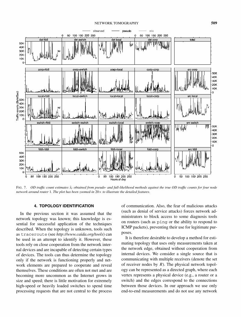
First, to compare with results presented by Cao et al.(2000a) we analyzed the same raw network OD trafficdata collected on February 22, 1999 for the Router 1network depicted in Figure 5b. Figures 6 and 7 showthe estimated OD traffic from MPLE and MLE basedon the link traffic for the subnetwork along with thevalidation OD traffic via NetFlow. Figure 6 gives thefull scale plot and Figure 7 is the zoomed-in scale(20×). From the plot we can see that estimated ODtraffic from both MPLE and MLE agrees well withthe NetFlow measured OD traffic for large measure-ments, but not so well for small measurements wherethe Gaussian model is a poor approximation. From thepoint of view of origin–destination traffic engineering,it is adequate that the large traffic flows are inferredaccurately. For tasks such as planning and provision-ing activities, OD traffic estimates can then be used as
508 R. CASTRO, M. COATES, G. LIANG, R. NOWAK AND B. YU
FIG. 6. Full scale OD traffic count estimates x̂t obtained from pseudo- and full-likelihood methods against the true OD traffic counts forfour node network around router 1.
inexpensive substitutes for direct measurements. Theperformances of MPLE and MLE are comparable inthis case, but the computation of the MPLE is fasterthan MLE. For this example, the computations are car-ried out using R 1.5.0 (Ihaka and Gentleman, 1996)on a 1-GHz laptop: it takes about 12 s to compute theMPLE and about 49 s to compute the MLE in produc-ing Figure 6.
Second, to assess the performance of MPLE morethoroughly, simulations were carried out on somelarger networks through the network simulator ns-2(http://www.isi.edu/nsnam/ns). The experimental net-work topologies are (i) the two-router network depictedin Figure 5c and (ii) the Lucent network illustrated inFigure 5a, which comprises 21 end nodes and 27 links.From the simulation results (plots not shown), we seethat both pseudo- and full-likelihood methods capture
the dynamics of the simulated OD traffic under thezoomed-in scale. Table 1 summarizes the executiontime for both pseudo- and full-likelihood approachesunder the three different settings. From the tablewe can see that the pseudo-likelihood approach speedsup the computation without losing much estimationperformance, so it is more scalable to larger networks.
TABLE 1Execution times of MPLE and MLE on router networks of
different sizes
Network Number of MPLE MLEtopology edge nodes time (s) time (s)
FIG. 7. OD traffic count estimates x̂t obtained from pseudo- and full-likelihood methods against the true OD traffic counts for four nodenetwork around router 1. The plot has been zoomed-in 20× to illustrate the detailed features.
4. TOPOLOGY IDENTIFICATION
In the previous section it was assumed that thenetwork topology was known; this knowledge is es-sential for successful application of the techniquesdescribed. When the topology is unknown, tools suchas traceroute (see http://www.caida.org/tools) canbe used in an attempt to identify it. However, thesetools rely on close cooperation from the network inter-nal devices and are incapable of detecting certain typesof devices. The tools can thus determine the topologyonly if the network is functioning properly and net-work elements are prepared to cooperate and revealthemselves. These conditions are often not met and arebecoming more uncommon as the Internet grows insize and speed; there is little motivation for extremelyhigh-speed or heavily loaded switches to spend timeprocessing requests that are not central to the process
of communication. Also, the fear of malicious attacks(such as denial of service attacks) forces network ad-ministrators to block access to some diagnosis toolson routers (such as ping or the ability to respond toICMP packets), preventing their use for legitimate pur-poses.
It is therefore desirable to develop a method for esti-mating topology that uses only measurements taken atthe network edge, obtained without cooperation frominternal devices. We consider a single source that iscommunicating with multiple receivers (denote the setof receiver nodes by R). The physical network topol-ogy can be represented as a directed graph, where eachvertex represents a physical device (e.g., a router or aswitch) and the edges correspond to the connectionsbetween those devices. In our approach we use onlyend-to-end measurements and do not use any network
510 R. CASTRO, M. COATES, G. LIANG, R. NOWAK AND B. YU
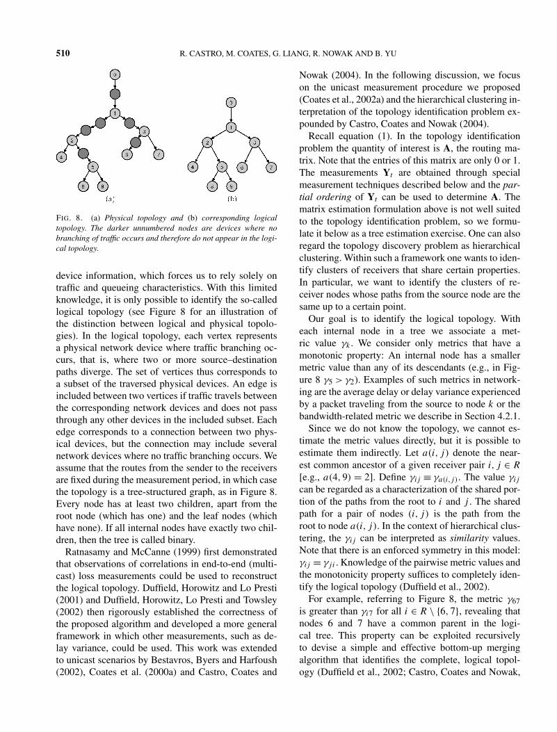
FIG. 8. (a) Physical topology and (b) corresponding logicaltopology. The darker unnumbered nodes are devices where nobranching of traffic occurs and therefore do not appear in the logi-cal topology.
device information, which forces us to rely solely ontraffic and queueing characteristics. With this limitedknowledge, it is only possible to identify the so-calledlogical topology (see Figure 8 for an illustration ofthe distinction between logical and physical topolo-gies). In the logical topology, each vertex representsa physical network device where traffic branching oc-curs, that is, where two or more source–destinationpaths diverge. The set of vertices thus corresponds toa subset of the traversed physical devices. An edge isincluded between two vertices if traffic travels betweenthe corresponding network devices and does not passthrough any other devices in the included subset. Eachedge corresponds to a connection between two phys-ical devices, but the connection may include severalnetwork devices where no traffic branching occurs. Weassume that the routes from the sender to the receiversare fixed during the measurement period, in which casethe topology is a tree-structured graph, as in Figure 8.Every node has at least two children, apart from theroot node (which has one) and the leaf nodes (whichhave none). If all internal nodes have exactly two chil-dren, then the tree is called binary.
Ratnasamy and McCanne (1999) first demonstratedthat observations of correlations in end-to-end (multi-cast) loss measurements could be used to reconstructthe logical topology. Duffield, Horowitz and Lo Presti(2001) and Duffield, Horowitz, Lo Presti and Towsley(2002) then rigorously established the correctness ofthe proposed algorithm and developed a more generalframework in which other measurements, such as de-lay variance, could be used. This work was extendedto unicast scenarios by Bestavros, Byers and Harfoush(2002), Coates et al. (2000a) and Castro, Coates and
Nowak (2004). In the following discussion, we focuson the unicast measurement procedure we proposed(Coates et al., 2002a) and the hierarchical clustering in-terpretation of the topology identification problem ex-pounded by Castro, Coates and Nowak (2004).
Recall equation (1). In the topology identificationproblem the quantity of interest is A, the routing ma-trix. Note that the entries of this matrix are only 0 or 1.The measurements Yt are obtained through specialmeasurement techniques described below and the par-tial ordering of Yt can be used to determine A. Thematrix estimation formulation above is not well suitedto the topology identification problem, so we formu-late it below as a tree estimation exercise. One can alsoregard the topology discovery problem as hierarchicalclustering. Within such a framework one wants to iden-tify clusters of receivers that share certain properties.In particular, we want to identify the clusters of re-ceiver nodes whose paths from the source node are thesame up to a certain point.
Our goal is to identify the logical topology. Witheach internal node in a tree we associate a met-ric value γk . We consider only metrics that have amonotonic property: An internal node has a smallermetric value than any of its descendants (e.g., in Fig-ure 8 γ5 > γ2). Examples of such metrics in network-ing are the average delay or delay variance experiencedby a packet traveling from the source to node k or thebandwidth-related metric we describe in Section 4.2.1.
Since we do not know the topology, we cannot es-timate the metric values directly, but it is possible toestimate them indirectly. Let a(i, j) denote the near-est common ancestor of a given receiver pair i, j ∈ R
[e.g., a(4,9) = 2]. Define γij ≡ γa(i,j). The value γij
can be regarded as a characterization of the shared por-tion of the paths from the root to i and j . The sharedpath for a pair of nodes (i, j) is the path from theroot to node a(i, j). In the context of hierarchical clus-tering, the γij can be interpreted as similarity values.Note that there is an enforced symmetry in this model:γij = γji . Knowledge of the pairwise metric values andthe monotonicity property suffices to completely iden-tify the logical topology (Duffield et al., 2002).
For example, referring to Figure 8, the metric γ67is greater than γi7 for all i ∈ R \ {6,7}, revealing thatnodes 6 and 7 have a common parent in the logi-cal tree. This property can be exploited recursivelyto devise a simple and effective bottom-up mergingalgorithm that identifies the complete, logical topol-ogy (Duffield et al., 2002; Castro, Coates and Nowak,
NETWORK TOMOGRAPHY 511
2004). These same techniques are used in agglom-erative hierarchical clustering methods (Ward, 1963;Willet, 1988; Fasulo, 1999).
In general, we do not have access to the exact pair-wise metric values and can only observe a noisy anddistorted version of them, usually obtained by activelyprobing the network. If we have a statistical model thatrelates the underlying (unknown) metric values and themeasurements, we can formulate the topology identi-fication problem as a maximum-likelihood estimationexercise.
For a given unknown tree T with a receiver set R,let Xij be a random variable parameterized by γij forany i, j ∈ R, i = j , and let γ = {γij }. Let p(x|γ ) de-note the joint probability density function of those ran-dom variables. A sample x ≡ {xij : i, j ∈ R, i = j}of the random variables Xij is observed. These arethe pairwise measurements recorded through a probingprocess such as the one described in Section 4.2.1. Themaximum-likelihood tree estimate is then given by
T ∗(x) = arg maxT ∈F
supγ∈G(T )
p(x|γ ),(8)
where F denotes the forest of all possible trees withleaves R, and G(T ) is the set of all γ ’s that satisfythe monotonicity property for the tree T . In many sit-uations we are not interested in estimating γ ; hence,we can regard γ as nuisance parameters. In that case,(8) can be interpreted as a maximization of the profilelikelihood (Berger, Liseo and Wolpert, 1999)
L(x|T ) ≡ supγ∈G(T )
p(x|γ ).(9)
The solution of (8) is referred to as the maximum-likelihood tree (MLT).
Under reasonable modeling assumptions the randomvariables Xij are independent. Taking this into accountyields a useful factorization of the log-likelihood. As-sume that the random variables Xij have densitiesp(xij |γij ), i, j ∈ R, i = j , with respect to a commondominating measure. Let fij (xij |γij ) = logp(xij |γij ).The log-likelihood is then
logp(x|γ ) = ∑i∈R
∑j∈R\{i}
fij (xij |γij ).(10)
The optimization problem in (8) is quite formidable.We are not aware of any method for computation ofthe global maximum except by a brute force exami-nation of each tree in the forest. Consider a tree with
N leaves. A very loose lower bound on the size ofthe forest F is N !/2. For example, if N = 10, thenthere are more than 1.8 × 10⁶ trees in the forest. More-over, the computation of the profile likelihood (9) isnontrivial because it involves a constrained optimiza-tion over G(T ). Castro, Coates and Nowak (2004)showed that if the functions fij are concave, it isnot necessary to perform the constrained optimization,since the maximum-likelihood metric value estimatefor the MLT is always in the interior of the set G(T ).Hence one can just compute an unconstrained opti-mization and subsequently check if the resulting max-imizer lies in the set G(T ). However, even with thissimplification, it is still infeasible to search exhaus-tively over all candidate trees. In the following sub-sections we briefly describe two alternative algorithmsthat return tree estimates that are an approximation tothe MLT.
4.1.1 Bottom-up agglomerative procedure. In a sce-nario where one can determine the true pairwise sim-ilarity metrics γ , it is possible to reconstruct the treetopology using a simple agglomerative bottom-up pro-cedure (Willet, 1988; Duffield et al., 2002). Whenwe only have access to the measurements x, convey-ing indirect information about γ , we can still developa bottom-up agglomerative clustering algorithm to es-timate the true topology. This method follows the sameconceptual framework as many hierarchical clusteringtechniques, and proceeds by repeatedly applying foursteps:
1. Choose the pair of nodes with the highest similarity.2. Merge the pair into a new node/cluster.3. Update the similarities between the new node and
the former existing nodes.4. Repeat the procedure until only one node is left.
The crucial step is the update of the similarity val-ues, and in many hierarchical clustering algorithms theupdate procedure is chosen via application-dependentheuristics (Fasulo, 1999). In our model-based ap-proach, which relates γ to x, the appropriate updateof similarities arises naturally from the likelihood for-mulation and leads to the agglomerative likelihood tree(ALT) algorithm (Castro, Coates and Nowak, 2004).
The algorithm commences by considering a set ofnodes S, initialized to the receiver set R, and formingthe estimates of the pairwise similarity metrics for eachpair of nodes in the set S, given by
γ̂ij = arg maxγ∈R
(fij (xij |γ ) + fji(xji |γ )
),
(11)i, j ∈ S, i = j.
512 R. CASTRO, M. COATES, G. LIANG, R. NOWAK AND B. YU
One expects the above estimated pairwise similaritiesto be reasonably close to the true similarities γ . Con-sider the pair of nodes such that γ̂ij is greatest, that is,
γ̂ij ≥ γ̂lm, ∀ l,m ∈ S.
We infer that i and j are the most similar nodes, im-plying that they have a common parent k in the tree.
Assuming that our decision is correct, the tree struc-ture and the likelihood impose some structure on thetrue similarities, providing a logical way to perform themerging of similarities (see Castro, Coates and Nowak,2004, for details). The algorithm proceeds by replac-ing nodes i and j with their parent k in S. For a givennode k, we denote by Rk the set of receivers which aredescendants of k in the tree. Thus, at the initial stageof the algorithm Ri = {i}, and after the update step,Rk = Ri ∪ Rj . We update the similarity estimates in Saccording to
γ̂kl = γ̂lk ≡ arg maxγ∈R
∑r∈Rk
frl(xrl|γ ) + flr (xlr |γ ),
(12)where l ∈ S \ {k}.
These two steps, selecting the pair of nodes with max-imum estimated similarity for merger and updating thesimilarities, are repeated until there is a single nodein S. Castro, Coates and Nowak (2004) formalized theconcepts behind this algorithm and showed that if theunderlying tree is binary and the estimated pairwisesimilarities are sufficiently close to the true similari-ties, then the ALT algorithm is equivalent to the MLTand identifies the true topology.
4.1.2 Markov chain Monte Carlo approach. De-spite the simplicity of the ALT algorithm, it is a greedyprocedure based on local decisions that involve the es-timated pairwise similarities. If an incorrect local de-cision is made at some stage in the algorithm, then itcannot be reversed. In the topology estimation prob-lem the measurement process is generally distributed,relying on clocks and counters at numerous networksites. It is frequently the case that several of the mea-surements are substantially more inaccurate than therest. The ALT algorithm compares pairwise similarityestimates, each of which is formed from only a subsetof the available measurements and is thus vulnerableto the effect of the local inaccuracies. Unlike the ALT,the MLT estimator takes a global approach: the expres-sion to be optimized in (8) involves a contribution fromall of the measurements, and identification of the MLTrequires a simultaneous consideration of all the pair-wise similarities. The price to pay is that identification
of the MLT involves a search over the entire forest F .In this section we propose a random search techniquethat efficiently searches the forest of trees and, mostimportantly, focuses on the likely regions of the forest.
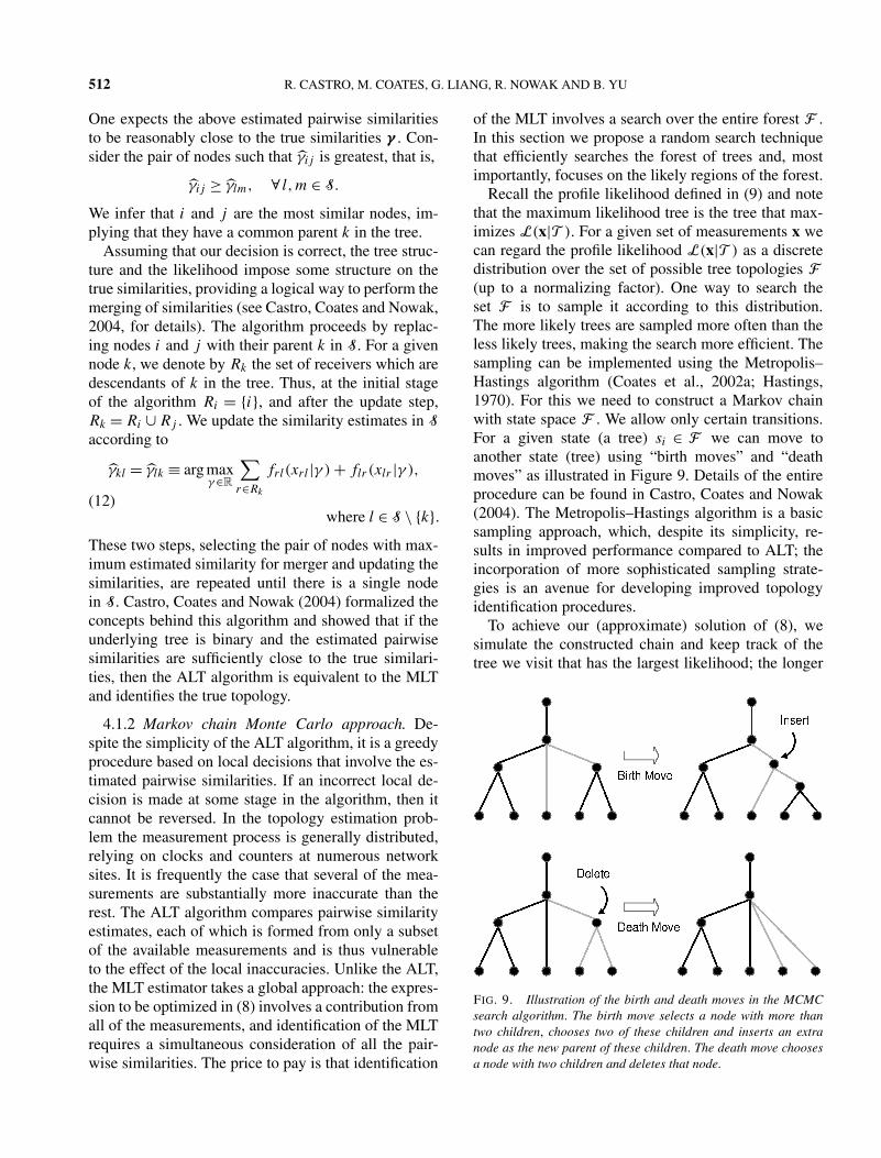
Recall the profile likelihood defined in (9) and notethat the maximum likelihood tree is the tree that max-imizes L(x|T ). For a given set of measurements x wecan regard the profile likelihood L(x|T ) as a discretedistribution over the set of possible tree topologies F(up to a normalizing factor). One way to search theset F is to sample it according to this distribution.The more likely trees are sampled more often than theless likely trees, making the search more efficient. Thesampling can be implemented using the Metropolis–Hastings algorithm (Coates et al., 2002a; Hastings,1970). For this we need to construct a Markov chainwith state space F . We allow only certain transitions.For a given state (a tree) si ∈ F we can move toanother state (tree) using “birth moves” and “deathmoves” as illustrated in Figure 9. Details of the entireprocedure can be found in Castro, Coates and Nowak(2004). The Metropolis–Hastings algorithm is a basicsampling approach, which, despite its simplicity, re-sults in improved performance compared to ALT; theincorporation of more sophisticated sampling strate-gies is an avenue for developing improved topologyidentification procedures.
To achieve our (approximate) solution of (8), wesimulate the constructed chain and keep track of thetree we visit that has the largest likelihood; the longer
FIG. 9. Illustration of the birth and death moves in the MCMCsearch algorithm. The birth move selects a node with more thantwo children, chooses two of these children and inserts an extranode as the new parent of these children. The death move choosesa node with two children and deletes that node.
NETWORK TOMOGRAPHY 513
the chain is simulated, the higher the chance of visitingthe MLT at least once. Although theoretically the start-ing point (initial state) of the chain is not important,provided that the chain is simulated for long enough,starting at a reasonable point improves the chance ofvisiting the MLT in a reasonable simulation period.Starting the chain simulation from the tree obtained us-ing the ALT algorithm is a reasonable approach, sincethis is a consistent estimator and so one expects the re-sulting tree to be “close” (in terms of the number ofMCMC moves) to the actual MLT. This is the majorreason the simple Metropolis–Hastings sampling pro-cedure works reasonably well. Although inefficienciescan prevent it from visiting more than a small regionof the forest, it does visit much of the region near theMLT early in its evolution and can thus “correct” localerrors in the ALT.
One drawback to the likelihood criterion is that itplaces no penalty on the number of links in the tree. Asa consequence, trees with more links can have higherlikelihood values (since the extra degrees of freedomthey possess allow them to fit the data more closely).This is an instance of the classic “overfitting” problemassociated with model estimation (Rissanen, 1989) andcan be remedied by applying regularization, that is, byreplacing the simple likelihood criterion with a penal-ized likelihood criterion,
T̂λ = arg maxT ∈F
logL(x|T ) − λn(T ),(13)
where n(T ) is the number of links in the tree T andλ ≥ 0 is a parameter, chosen by the user, to balancethe trade-off between fitting to the data and control-ling the number of links in the tree. We can use anMCMC method in a similar fashion as before to ap-proximately find the solution of (13). Minimum de-scription length principles (Rissanen, 1989) motivatea penalty that is dependent on the size of the network(in terms of the number of receivers). However, othermodel selection techniques lead to choices of differentpenalties (Robert and Casella, 1999).
4.2 Experimental Results
4.2.1 Probing techniques and modeling. There areseveral possible choices for similarity metrics in thetopology identification problem; the only constraintsare that the metric obey the monotonicity propertyand is measurable in a practical setting. It is possibleto devise similarity metrics that rely on packet losses(e.g., average loss on a shared path). Although these
are appealing because they are very simple to mea-sure, losses are relatively rare in a properly function-ing network (generally less than 2% for an end-to-endpath), so these metrics have poor discrimination prop-erties. Metrics that use delay/timing measurements of-fer better discrimination (Duffield, Horowitz and LoPresti, 2001), but their estimation often requires clocksynchronization between various physical points in thenetwork, a rather difficult task (Pásztor and Veitch,2002). In earlier work we proposed a topology iden-tification method based on delay differences (Coateset al., 2002a). The measurement technique overcomesthe clock synchronization issues without impairing thegood discrimination of delay-based metrics and henceit is easily deployed in practice. The method relies on ameasurement scheme called sandwich probing, detailsof which can be found in Coates et al. (2002a); here wepresent a brief overview.
Each sandwich probe consists of three packets andgives information about the shared path between tworeceivers. Figure 10 illustrates the probing scheme. Thelarge packet is destined for node 2; the small packetsare destined for node 3. The black circles on the linksrepresent physical queues where no branching occurs.The initial spacing between the small probes d is in-creased along the shared path from nodes 0 to 1 be-cause the second small probe p2 queues behind thelarge packet (due to the bandwidth limitations of eachlink). The measurement collected for each receiver pairis the extra delay difference �d between the two smallpackets. This extra delay is due to the queueing of thesecond small packet behind the large one, for all linksin the shared portion of the path. The metric used foreach pair is the mean delay difference. In idealized net-work conditions (Coates et al., 2002a), the contribution
FIG. 10. Example of sandwich probe measurement.
514 R. CASTRO, M. COATES, G. LIANG, R. NOWAK AND B. YU
from each link in the shared path to the mean delay dif-ference is inversely proportional to its bandwidth and isalways positive, so the metric satisfies the monotonic-ity property.
The observed mean delay differences are noisy ver-sions of the underlying metrics, primarily because ofthe influence of background traffic in the network.Let xij be the sample mean of repeated delay differ-ence measurements for pair i, j ∈ R. We assume thatthe cross-traffic is stationary over the measurement in-terval and the initial spacing of the two small pack-ets d is large enough so that neither the large packetnor the second small packet queues behind the firstsmall packet at any time. We send each probe far apartin time, so we can assume that the outcomes of dif-ferent measurements are independent. Under these andother mild assumptions, the measurements are statisti-cally independent and have finite variance; hence, ac-cording to the central limit theorem, the distribution ofeach empirical mean tends to a Gaussian. This moti-vates the (approximate) model
xij ∼ N (γij , σ2ij ),(14)
where σ 2ij is the sample variance of the measurements,
divided by the number of measurements xij is the sam-ple mean of the measurements and N (γ, σ 2) denotesthe Gaussian density with mean γ and variance σ 2.Notice that we are not assuming that the delay differ-ences are normally distributed, but only their empiricalmeans. Under the above assumptions, as the number ofmeasurements increases, the model accuracy increases.We also assume that the measurements for the differ-ent receiver pairs are statistically independent, whichis a reasonable assumption due to generally weak spa-tial correlation between traffic on different links.
4.2.2 Internet experiments. We have implemented asoftware tool called nettomo that performs sandwichprobing measurements and estimates the topology ofa tree-structured network. We conducted Internet ex-periments using several hosts in the United States andabroad. The topology inferred from tracerouteis depicted in Figure 11a. Often the traceroutetool cannot be used to determine the topology, but itdoes work in this measurement scenario and thus pro-vides a useful ground truth for validation (even here,traceroute fails to detect one network element).The source for the experiments was located at RiceUniversity. There are 10 receiver clients, 2 locatedon different networks at Rice, 2 at separate hosts inPortugal and 6 located at four other U.S. universities.
(a)
(b)
(c)
FIG. 11. (a) The topology of the network used for Internet ex-periments obtained using traceroute. (b) Estimated topologyusing the ALT algorithm. The three links inside the ellipse havelink-parameter values γk − γf (k) that are one order of magnitudesmaller than all the other links. (c) The estimated topology obtainedusing the MCMC method with a penalized likelihood criterion.
The experiment was conducted for a period of 8 min,during which a sandwich probe was sent to a ran-domly chosen receiver pair once every 50 ms. With-out any loss, the maximum number of probes availableis 8600. This corresponds to less than 200 probes perpair; hence the traffic overhead on any link is very low.
NETWORK TOMOGRAPHY 515
We applied the ALT algorithm to the measurementscollected and the result is depicted in Figure 11b. Sincethe procedure is suited only for binary trees, it addssome extra links with small link-level metric value (i.e.,γk − γf (k) ≈ 0). The extra links are an artifact of ourmodel and are essentially overfitting the data. Usingthe maximum penalized likelihood approach, we ob-tain the result depicted in Figure 11c (see Coates et al.,2002a, for details of the penalty selection procedure).Notice that this is very close to the traceroutetopology, but it fails to detect the backbone connec-tion between Texas and Indianapolis. We expect thatthe latter connection is very high speed and that thequeuing effects on the constituent links are too minorto influence measurements sufficiently for its detection.The estimated topologies also place an extra shared el-ement between the Rice computers. This element is nota router and hence is not shown in the topology re-turned by traceroute, but it corresponds to a realphysical device and branching point. To the best of ourknowledge, the detected element is a bandwidth limi-tation device.
5. CONCLUSION AND FUTURE DIRECTIONS
This article has provided an overview of the areaof large-scale inference and tomography in commu-nication networks. As is evident from the limitedscale of the simulations and experiments discussedin this article, the field is emerging. Deploying mea-surement/probing schemes and evaluating inferencealgorithms for larger networks is the next key step.Statistics will continue to play an important role inthis area and in this section we attempt to stimulatethe reader with an outline of some of the many openissues. These issues can be divided into extensions ofthe theory and potential networking application areas.
The spatiotemporally stationary and independenttraffic and network transport models that currentlydominate network tomography research have limi-tations, especially in tomographic applications thatinvolve heavily loaded networks. Since one of the prin-cipal applications of network tomography is to detectheavily loaded links and subnets, relaxation of theseassumptions continues to be of great interest. Somerecent work on relaxing spatial dependence and tem-poral independence has appeared in unicast (Shih andHero, 2001) and multicast (Cáceres et al., 1999) set-tings. However, we are far from the point of being ableto implement flexible yet tractable models which si-multaneously account for long time traffic dependence,
latency, dynamic random routing and spatial depen-dence. As wireless links and ad hoc networks becomemore prevalent, accounting for spatial dependence androuting dynamics will become increasingly important.
Recently there have been some preliminary attemptsto deal with the time-varying, nonstationary nature ofnetwork behavior. In addition to the estimation of time-varying OD traffic matrices discussed in Section 3.2,other researchers have adopted a dynamical systemsapproach to handle nonstationary link-level tomogra-phy problems (Coates and Nowak, 2002). SequentialMonte Carlo inference techniques were employed byCoates and Nowak (2002) to track time-varying linkdelay distributions in nonstationary networks. Onecommon source of temporal variability in link-levelperformance is the nonstationary characteristics ofcross-traffic.
There is also an accelerating trend toward networksecurity that will create a highly uncooperative en-vironment for active probing—firewalls designed toprotect information may not honor requests for rout-ing information, special packet handling (multicast,TTL, etc.) and other network transport protocols re-quired by many current probing techniques. This hasprompted investigations into more passive traffic mon-itoring techniques, for example, based on samplingTCP traffic streams (Padmanabhan, Qiu and Wang,2002; Tsang, Coates and Nowak, 2001). Furthermore,the ultimate goal of carrying out network tomographyon a massive scale poses a significant computationalchallenge. Decentralized processing and data fusionwill probably play an important role in reducing boththe computational burden and the high communica-tion overhead of centralized data collection from edgenodes.
The majority of work reported to date has focusedon reconstruction of network parameters which maybe only indirectly related to the decision-making ob-jectives of the end-user regarding the existence ofanomalous network conditions. An example of thisis bottleneck detection considered by Shih and Hero(2001) and Ziotopolous, Hero and Wasserman (2001)as an application of reconstructed delay or loss esti-mation. Other important decision-oriented applicationsmay be detection of coordinated attacks on network re-sources, network fault detection and verification of ser-vices.
Finally, the impact of network monitoring, which isthe subject of this article, on network control and pro-visioning could become the application area of mostpractical importance. Admission control, flow control,
516 R. CASTRO, M. COATES, G. LIANG, R. NOWAK AND B. YU
service level verification, service discovery and effi-cient routing could all benefit from up-to-date andreliable information about link and router level perfor-mances. The big question is, Can statistical methods bedeveloped which ensure accurate, robust and tractablemonitoring for the development and administration ofthe Internet and future networks?
ACKNOWLEDGMENTS
This work was supported by National Science Foun-dation Grants MIP–97-01692, ANI-00-99148, FD-01-12731 and ANI-97-34025, Office of Naval ResearchContract N00014-00-1-0390, Army Research OfficeGrants DAAD19-99-1-0290, DAAD19-01-1-0643 andDAAH04-96-1-0337, Science and Engineering Re-search Canada, and Department of Energy Grant DE-FC02-01ER25462. We acknowledge the invaluablecontributions of J. Cao, D. Davis, M. Gadhiok, R. King,E. Rombokas, Y. Tsang and S. Vander Wiel to the workdescribed in this article.
REFERENCES
BERGER, J. O., LISEO, B. and WOLPERT, R. L. (1999). Integratedlikelihood methods for eliminating nuisance parameters (withdiscussion). Statist. Sci. 14 1–28.
BESAG, J. (1974). Spatial interaction and the statistical analysis oflattice systems (with discussion). J. Roy. Statist. Soc. Ser. B 36192–236.
BESAG, J. (1975). Statistical analysis of non-lattice data. The Sta-tistician 24 179–195.
BESTAVROS, A., BYERS, J. and HARFOUSH, K. (2002). Inferenceand labeling of metric-induced network topologies. In Proc.IEEE INFOCOM 2002 2 628–637. IEEE Press, New York.
BLACKWELL, D. (1973). Approximate normality of large products.Technical report, Dept. Statistics, Univ. California, Berkeley.
CÁCERES, R., DUFFIELD, N., HOROWITZ, J. and TOWSLEY, D.(1999). Multicast-based inference of network-internal losscharacteristics. IEEE Trans. Inform. Theory 45 2462–2480.
CAO, J., DAVIS, D.,VANDER WIEL, S. and YU, B. (2000a). Time-varying network tomography: Router link data. J. Amer. Statist.Assoc. 95 1063–1075.
CAO, J., VANDER WIEL, S., YU, B. and ZHU, Z. (2000b). A scal-able method for estimating network traffic matrices. Technicalreport, Bell Labs.
CASTRO, R., COATES, M. and NOWAK, R. (2004). Likelihoodbased hierarchical clustering. IEEE Trans. Signal Process. 522308–2321.
CHAO, X., MIYAZAWA, M. and PINEDO, M. (1999). QueueingNetworks: Customers, Signals and Product Form Solutions.Wiley, New York.
COATES, M., CASTRO, R., NOWAK, R., GADHIOK, M.,KING, R. and TSANG, Y. (2002a). Maximum likelihoodnetwork topology identification from edge-based unicastmeasurements. In Proc. ACM SIGMETRICS 2002 11–20.ACM Press, New York.
COATES, M., HERO, A., NOWAK, R. and YU, B. (2002b). Internettomography. IEEE Signal Processing Magazine 19(3) 47–65.
COATES, M. and NOWAK, R. (2000). Network loss inference usingunicast end-to-end measurement. In Proc. ITC Seminar on IPTraffic, Measurement and Modelling 28-1–28-9. Available atciteseer.ist.psu.edu/context/1699850/514748.
COATES, M. and NOWAK, R. (2002). Sequential Monte Carlo in-ference of internal delays in nonstationary communication net-works. IEEE Trans. Signal Process. 50 366–376.
COX, D. R. (1975). Partial likelihood. Biometrika 62 269–276.CSISZÁR, I. (1975). I -divergence geometry of probability distrib-
utions and minimization problems. Ann. Probab. 3 146–158.DUFFIELD, N., HOROWITZ, J. and LO PRESTI, F. (2001). Adaptive
multicast topology inference. In Proc. IEEE INFOCOM 20013 1636–1645. IEEE Press, New York.
DUFFIELD, N., HOROWITZ, J., LO PRESTI, F. and TOWSLEY, D.(2002). Multicast topology inference from measured end-to-end loss. IEEE Trans. Inform. Theory 48 26–45.
DUFFIELD, N., LO PRESTI, F., PAXSON, V. and TOWSLEY, D.(2001). Inferring link loss using striped unicast probes. InProc. IEEE INFOCOM 2001 2 915–923. IEEE Press, NewYork.
FASULO, D. (1999). An analysis of recent work on clustering al-gorithms. Technical Report 01-03-02, Dept. Computer Sci-ence and Engineering, Univ. Washington. Available at citeseer.nj.nec.com/fasulo99analysi.html.
HARFOUSH, K., BESTAVROS, A. and BYERS, J. (2000). Robustidentification of shared losses using end-to-end unicast probes.In Proc. IEEE International Conference on Network Protocols22–33. IEEE Press, New York. Errata available as TechnicalReport 2001-001, Dept. Computer Science, Boston Univ.
HASTINGS, W. (1970). Monte Carlo sampling methods usingMarkov chains and their applications. Biometrika 57 97–109.
IHAKA, R. and GENTLEMAN, R. (1996). R: A language for dataanalysis and graphics. J. Comput. Graph. Statist. 5 299–314.
KELLY, F. P., ZACHARY, S. and ZIEDINS, I., eds. (1996). Stochas-tic Networks: Theory and Applications. Oxford Univ. Press.
LELAND, W., TAQQU, M., WILLINGER, W. and WILSON, D.(1994). On the self-similar nature of Ethernet traffic.IEEE/ACM Transactions on Networking 2 1–15.
LIANG, G. and YU, B. (2003a). Maximum pseudo likelihood es-timation in network tomography. IEEE Trans. Signal Process.51 2043–2053.
LIANG, G. and YU, B. (2003b). Pseudo likelihood estimation innetwork tomography. In Proc. IEEE INFOCOM 2003 3 2101–2111. IEEE Press, New York.
LO PRESTI, F., DUFFIELD, N., HOROWITZ, J. and TOWSLEY, D.(2002). Multicast-based inference of network-internal de-lay distributions. IEEE/ACM Transactions on Networking 10761–775.
MORRIS, R. and LIN, D. (2000). Variance of aggregated web traf-fic. In Proc. IEEE INFOCOM 2000 1 360–366. IEEE Press,New York.
O’SULLIVAN, F. (1986). A statistical perspective on ill-posed in-verse problems (with discussion). Statist. Sci. 1 502–527.
PADMANABHAN, V. N., QIU, L. and WANG, H. (2002). Passivenetwork tomography using Bayesian inference. In Proc. ACMSIGCOMM Workshop on Internet Measurement 93–94. ACMPress, New York.
NETWORK TOMOGRAPHY 517
PÁSZTOR, A. and VEITCH, D. (2002). PC based precision timingwithout GPS. In Proc. ACM SIGMETRICS 2002 1–10. ACMPress, New York.
RATNASAMY, S. and MCCANNE, S. (1999). Inference of multi-cast routing trees and bottleneck bandwidths using end-to-endmeasurements. In Proc. IEEE INFOCOM 1999 1 353–360.IEEE Press, New York.
RISSANEN, J. (1989). Stochastic Complexity in Statistical Inquiry.World Scientific, Singapore.
ROBERT, C. and CASELLA, G. (1999). Monte Carlo StatisticalMethods. Springer, New York.
ROLLS, D. (2003). Limit theorems and estimation for structural andaggregate teletramc models. Ph.D. dissertation, Queen’s Univ.,Kingston, Ontario, Canada.
SCOTT, D. (1992). Multivariate Density Estimation: Theory, Prac-tice and Visualization. Wiley, New York.
SHIH, M. and HERO, A. (2001). Unicast inference of network linkdelay distributions from edge measurements. In Proc. IEEEInternational Conference on Acoustics, Speech, and SignalProcessing 6 3421–3424. IEEE Press, New York.
TEBALDI, C. and WEST, M. (1998). Bayesian inference on net-work traffic using link count data (with discussion). J. Amer.Statist. Assoc. 93 557–576.
TSANG, Y., COATES, M. and NOWAK, R. (2001). Passive networktomography using EM algorithms. In Proc. IEEE InternationalConference on Acoustics, Speech, and Signal Processing 31469–1472. IEEE Press, New York.
TSANG, Y., COATES, M. J. and NOWAK, R. (2003). Network delaytomography. IEEE Trans. Signal Process. 51 2125–2136.
VANDERBEI, R. J. and IANNONE, J. (1994). An EM approach toOD matrix estimation. Technical Report SOR 94-04, Prince-ton Univ.
VARDI, Y. (1996). Network tomography: Estimating source-destination traffic intensities from link data. J. Amer. Statist.Assoc. 91 365–377.
WARD, J. H. (1963). Hierarchical grouping to optimize an objectivefunction. J. Amer. Statist. Assoc. 58 236–245.
WHITE, H. (1994). Estimation, Inference and Specification Analy-sis. Cambridge Univ. Press, New York.
WILLET, P. (1988). Recent trends in hierarchical document clus-tering: A critical review. Information Processing and Manage-ment 24 577–597.
ZIOTOPOLOUS, A., HERO, A. and WASSERMAN, K. (2001). Es-timation of network link loss rates via chaining in multicasttrees. In Proc. IEEE International Conference on Acoustics,Speech, and Signal Processing 4 2517–2520. IEEE Press,New York.