33
Statistical Techniques I EXST7005 Conceptual Intro to ANOVA
| Date post: | 27-Dec-2015 |
| Category: |
Documents |
| Upload: | loraine-shana-lloyd |
| View: | 217 times |
| Download: | 0 times |

Statistical Techniques IEXST7005
Conceptual Intro to ANOVA

Analysis of Variance (ANOVA)
R. A. Fisher - resolved a problem that had existed for some time.
H0: 1 = 2 = 3 = ... = k H1: some i is different Conceptually, we have separate (and independent) samples, each giving a mean, and we want to know if they could have come from the same population or if is more likely they come from different populations.

The Problem (continued)
One way to do this is a series of t-tests. If we want to test among 3 means we do 3 tests: 1
versus 2, 1 versus 3, 2 versus 3For 4 means there are 6 tests. 1-2, 1-3, 1-4, 2-3, 2-
4, and 3-4For 5 means, 10 tests, etc.

The Problem (continued)
This technique is unwieldy, and worse. When we do the first test, there is an chance of error, and for each additional test another chance of error. So if you do 3 or 6 or 10 tests, the chance of error on each and every test is .
Overall, for the experiment, the chance of error for all tests together is much higher than .
The Problem (continued)
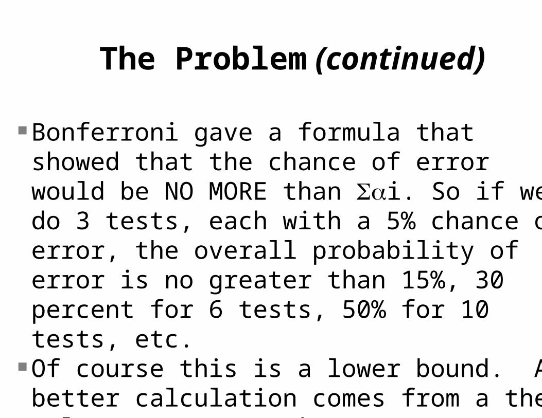
Bonferroni gave a formula that showed that the chance of error would be NO MORE than i. So if we do 3 tests, each with a 5% chance of error, the overall probability of error is no greater than 15%, 30 percent for 6 tests, 50% for 10 tests, etc.
Of course this is a lower bound. A better calculation comes from a the value. '=1-(1-)k.

No. of means
pairwise tests
Bonferroni's lower bound
Duncan's1-(1-)k
(1-)
2 1 0.05 0.0500 0.9503 3 0.15 0.1426 0.8574 6 0.30 0.2649 0.7355 10 0.50 0.4013 0.5996 15 0.75 0.5367 0.4637 21 1.05 0.6594 0.341
10 45 2.20 0.9006 0.09950 1225 61.20 0.9999 0.000
100 4950 247.45 1.0000 0.000
for = 0.05
The Problem (continued)
The bottom line: Splitting an experiment into a number of smaller tests is generally a poor idea. This applies at higher levels as well (i.e. splitting big ANOVAs into little ones).
The solution: We need ONE test that will give us an accurate test with an value of the desired level.

The concept
We are familiar with variance.

The concept (continued)
We are familiar with the pooled variance

The concept (continued)
We are familiar with the variance of the means. But we never get "multiple" estimates of the mean and calculate a mean from those. The one we use comes from statistical theory.

The concept (continued) Could we actually get multiple estimates of the means and calculate a sum of squared deviations of the various means from an overall mean and get variance of the means from that?

The concept (continued)
Yes, we could, and it should give the same value.

The concept (continued)
Suppose we have some values from a number of different samples, perhaps taken at different
places. The values would be Yij, where the places are i=1, 2, ..., k, and the observations
within places are j=1, 2, 3, ..., ni. For each site we calculate a value of the mean. We then take the various means (k different means) and calculate a variance among those. This would also give the "variance of the means".

The LOGIC Remember, we want to test H0: 1 = 2 = 3 = ... = k We have a bunch of means and we want to know if they were drawn from the same population or different populations.
We also have a bunch of samples each with its own variance (S2). If we can assume homogeneous variance (all variances equal) then we could POOL the multiple estimates of variance.
The LOGIC (continued)
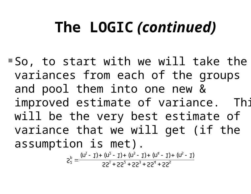
So, to start with we will take the variances from each of the groups and pool them into one new & improved estimate of variance. This will be the very best estimate of variance that we will get (if the assumption is met).

The LOGIC (continued)
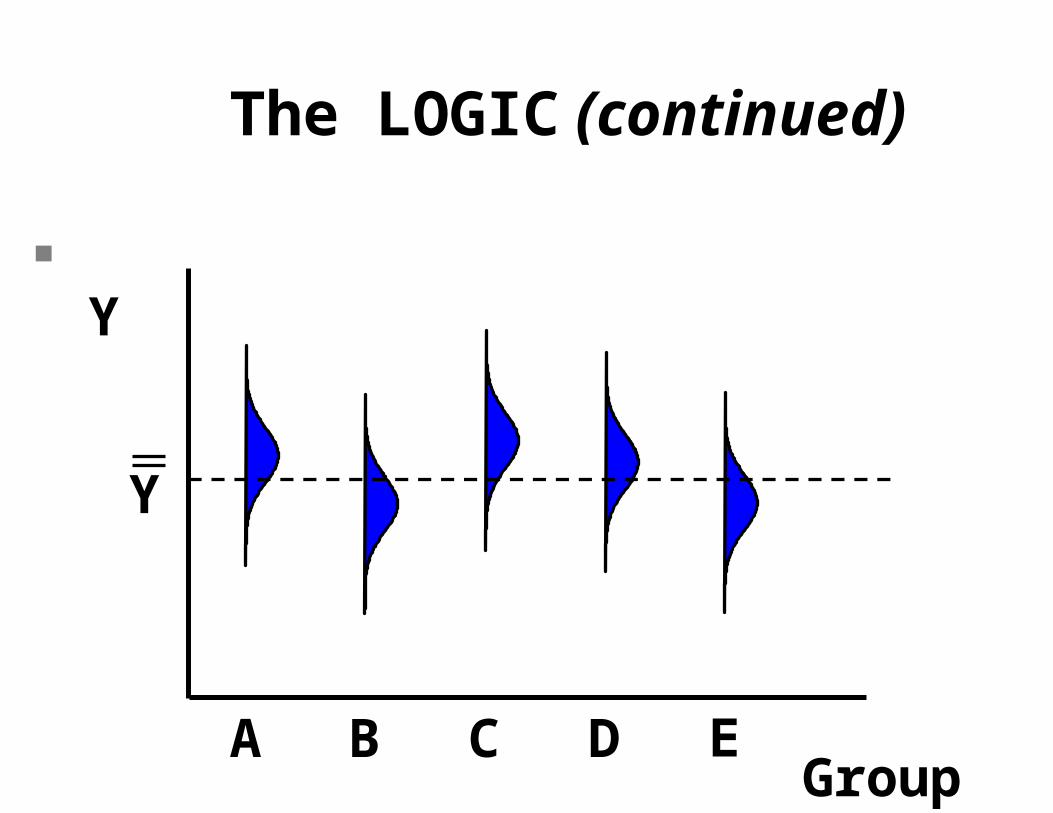
Now, think about the means. If the NULL HYPOTHESIS IS TRUE, then we could calculate the variance of the means from the means. This would estimated S2Y, the variance of the means. We would take the deviations of each Y from the overall mean, and get a variance from that.
Pictorially,

The LOGIC (continued)
Y
GroupA B C D E
Y
Means
Deviations

The LOGIC (continued)
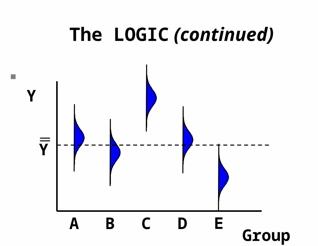
If the null hypothesis is true, the means should be pretty close to the overall mean. They won't be EXACTLY equal to the overall mean because of random sampling variation in the individual observations.
The LOGIC (continued)
Y
GroupA B C D E
Y

The LOGIC (continued)
However, if the null hypothesis is false, then some mean will be different! At least one, maybe several.
The LOGIC (continued)
Y
GroupA B C D E
Y

The LOGIC (continued)
So we take the Sum of squared deviations, divide by the degrees of freedom and we get an estimate of the variance of the means.

The LOGIC (continued)
But this does not exactly estimate the variance, it estimates the variance divided by the sample size! The sample size is the number of observations in each mean.

The LOGIC (continued)
In order to estimate the variance we must multiply this estimate by n, the sample size.

The LOGIC (continued)
This is obviously easier if each sample size is the same (i. e. the experiment is balanced). I will show the calculations for a balanced design, but the analysis can readily be done if the data is not balanced. It's just a little more complicated.

The Solution
So what have we got? One variance estimate that is pooled across all of
the samples because the variances are equal (an assumption, sometimes testable).
And another variance that should be the same if the null hypothesis is TRUE.
The second mean (from the variances) will not be the same if the null hypothesis is false.

The Solution (continued)
NOT only will the second variance from the mean not be the same, IT WILL BE LARGER!!!
Why? Because when we are testing means for equality we will not consider rejecting if the means are too similar, only if they are too different, and large differences yield large deviations which produce an overly large variance.
So this will be a one tailed test.
The Solution (continued)
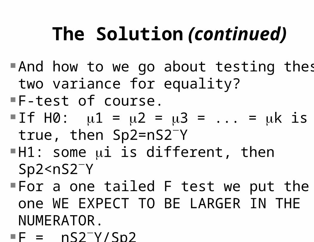
And how to we go about testing these two variance for equality?
F-test of course. If H0: 1 = 2 = 3 = ... = k is true, then Sp2=nS2Y
H1: some i is different, then Sp2<nS2Y For a one tailed F test we put the one WE EXPECT TO BE LARGER IN THE NUMERATOR.
F = nS2Y/Sp2

The Solution (continued)
And that is Analysis of Variance. We are actually testing means, but we are doing it by turning them into variances.
One pooled variance from within the groups, called the "pooled within variance".
And one from between groups or among groups called the "variance among groups".
The Solution (continued)
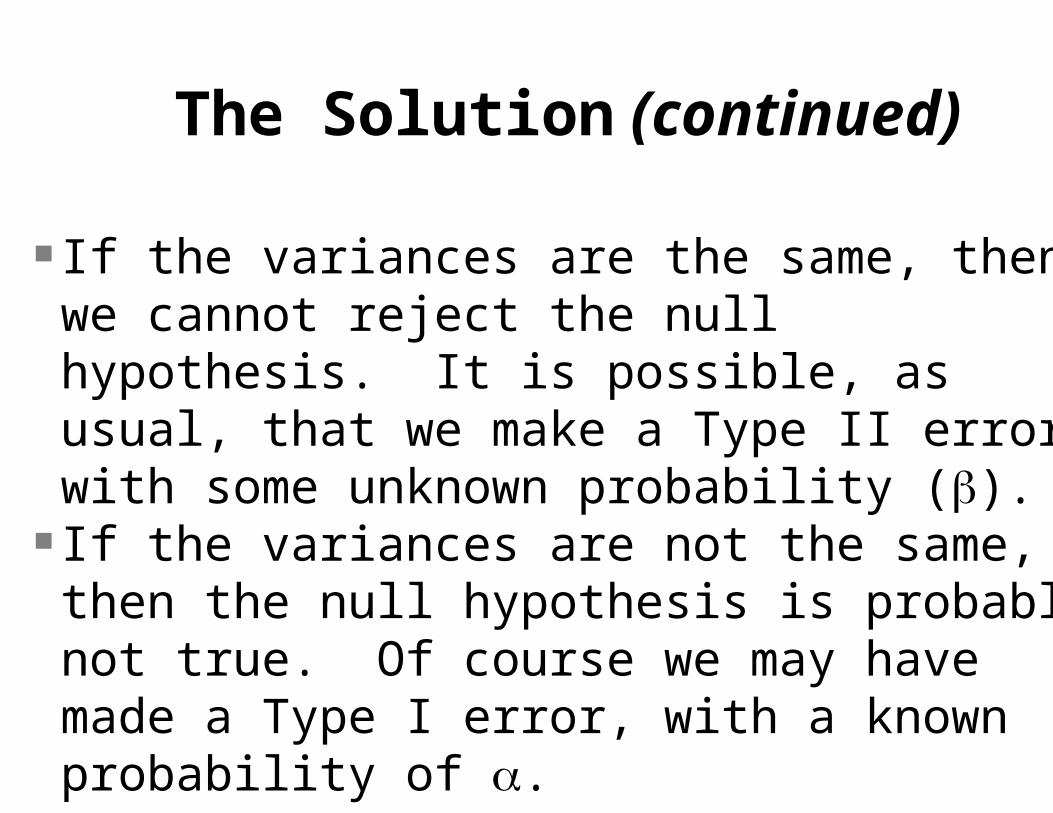
If the variances are the same, then we cannot reject the null hypothesis. It is possible, as usual, that we make a Type II error with some unknown probability ().
If the variances are not the same, then the null hypothesis is probably not true. Of course we may have made a Type I error, with a known probability of .

The Solution (continued)
All the math later, but this is the basic idea.

R. A. Fisher
Ronald Aylmer Fisher - the father of modern statistics.
Born in 1890 Very poor eyesight prevented him from learning by electric light, and had to learn by having things read out to him. He developed the ability to figure mathematical equations in his head.

R. A. Fisher (continued)
He left an academic position teaching mathematics for a position at Rothamsted Agricultural Experiment Station
In this environment he developed many applied analyses for testing experimental hypotheses, and provided much of the foundation for modern statistics.
We will see several other analyses developed by Fisher.


