Statistical Testing in Medical Education Research

Goutham Rao, MD

10 September 2010

Objectives

To provide an overview of numeracy and the importance of understanding statistical tests.

To review underlying principles of statistical tests.

To provide a review of the rationale, calculation, and applicability of common statistical tests.

Physician Numeracy

Clinical Epidemiology and Biostatistics

→ Introduction to Medical Decision Making

Physician Numeracy

“defined as understanding the statistical aspects of and terminology associated with the design, analysis, and results of original research. This includes, for example, having a general understanding of how the power of a study is calculated, or understanding the meaning of a confidence interval”.

Physician Numeracy Cont’d Core Principles: (1) Journal clubs have

important limitations. (2) Understanding the

quantitative aspects of research promotes an in-depth understanding of papers.

(3) Physician numeracy can form the basis of an EBM course.

(4) Consumers of original research ought to determine what is useful about a paper rather than whether or not it is useful.

(5) Numeracy should encompass only those concepts needed to accurately interpret evidence and apply it to individual patients.

Case Scenario #1

You have designed a new curriculum in palliative care, and wish to evaluate its impact upon fourth-year medical students. You randomized a class of 100 students to two groups: the new curriculum, which includes interactive case studies, small group sessions, and lectures; and the older curriculum which is purely didactic in nature. Both curricula are of the same duration. The primary outcome is students’ scores on a knowledge test consisting of 100 multiple-choice questions. You would like to know if the new curriculum is associated with greater gains in knowledge of palliative care.

Meltaway-Rx

Your friend Jack recently invented a new diet drug he calls “Meltaway-Rx.” He also evaluated this new drug in a study comparing it to two older drugs, A and B, among three groups of 5 patients. Below are the weight loss results for all 15 patients.

Results

Weight loss in 3 months (kg)

Drug A Drug B Meltaway-Rx

2 6 8

3 8 9

10 4 3

2 2 10

8 10 5

Is Meltaway-Rx superior?

We could take means.

Does not account for variation within groups.

Group differences could be due to treatment effects or simply due to individual or random variation.

Understanding differences

Differences can be “explainable”, i.e. the effect of being in a particular group.

Or, “unexplainable.”

If explained variation is significantly greater than unexplained variation, we can conclude that the three groups of subjects really are different. (i.e. The three treatments are not the same.)

Basic principle underlying all tests of significance

All based upon the ratio of,

Explained variation

Unexplained variation

If ratio is large, groups are statistically different; if small, groups are not statistically different.

Fundamental assessment of differences among groups

Analysis of variance (ANOVA)

Partitioning the variability (or differences)

Total sum of squares

SSTOTAL = (Xn – Grand mean) 2

Grand mean = 6

SSTOTAL = (2 – 6)2 + (3-6) 2 etc…. = 140

ANOVA (Cont’d)

Between groups differences (variability) given by,

SSBETWEEN GROUPS = n ( group mean – Grand mean)2

SSBETWEEN GROUPS = 5 * (5-6) 2 + (6-6) 2 + (7-6) 2 = 10

ANOVA (Cont’d)

SSWITHIN GROUPS = (X n- group mean)2

Easier to use the relationship, SSTOTAL = SSBETWEEN GROUPS +

SSWITHIN GROUPS

so that, SSWITHIN GROUPS = SSTOTAL - SSBETWEEN GROUPS

In our case SSWITHIN GROUPS = 140 –10 = 130.

ANOVA (Cont’d)

Sums of squares, like in the formulae for variance and standard deviation need to be divided by the df.

DF (Total) = total number of observations –1

DF (Between) = Total number of groups – 1

DF (Within) = Sum of total number of DFs in each group

Alternatively, DF (Total) = DF (Between) + DF (Within)

ANOVA (Cont’d)

By dividing sums of squares by DFs, we get mean squares.

MS (Between Groups) = SS (Between Groups) / DF (Between Groups)

MS (Within Groups) = SS (Within Groups)/ DF (Within

Groups)

For our case, MS (Between Groups) = 10/2 = 5

MS (Within Groups) = 130/12 = 10.8

ANOVA (Cont’d)

We now have measures of explained and unexplained differences. We simply calculate their ratio, which yields the F statistic:

F = MS (Between Groups)/MS (Within Groups) (0.46)

How big is a large F?

F follows a distribution under the assumption that there are no differences among groups. We can look and see how likely or probable we are to get a particular value of F if there were no differences among groups. If that probability is low, we say we have a big F.

Statistical Tests

All rely on basic ratio of explained to unexplained variation.

Choice of test depends upon type of data.

Values for test statistics are compared to values one would obtain under the assumption that there is no significant difference among groups being compared.

Comparisons to normal distribution in many cases.

What you need to know….

When individual tests should be used

The general principle(s) underlying each test

A general description of the procedures involved

Returning to Our Case Scenario

Randomized-controlled trial

There are two groups

Outcome is continuous

T-test

T Test

One of the most common statistical procedures.

Used to compare two groups of continuous data.

t = difference in sample meansstandard error of difference of sample means

T Test (Cont’d)

T becomes,

t = Ō – Ū

ÛÛÔÔ

2 s nsn

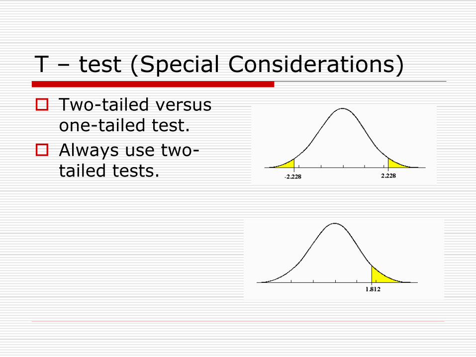
T – test (Special Considerations)

Two-tailed versus one-tailed test.

Always use two-tailed tests.

Case Scenario #2

We wish to determine if family income of medical students has an impact upon the choice of a primary care specialty for residency. We study 180 students.

The outcome is categorical and binary (chooses primary care or not).

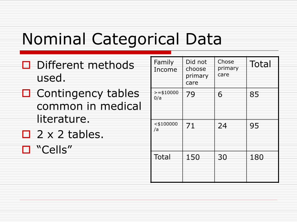
Nominal Categorical Data

Different methods used.

Contingency tables common in medical literature.

2 x 2 tables.

“Cells”

Family Income

Did not choose primary care

Chose primary care

Total

>=$100000/a

79 6 85

<$100000/a

71 24 95

Total 150 30 180

Chi-Squared Statistic

Χ2 = Σ {(observed – expected value of cell)2/ expected value of cell}

“Expected value” refers to the value we would expect assuming that income makes no difference. (i.e. The rate of choosing primary care does not differ between the two groups.)

Case (Cont’d)

30 people chose primary care among 180 subjects (16.67%).

If family income makes no difference, we would observe this same rate of of choosing primary care in both groups. .167 x 85 and .167 x 95.

We can reconstruct our 2 x 2 table with these expected values.

Chi-Squared Test (Cont’d)

Reconstruction with expected values in each cell.

Family Income

Did not choose primary care

Chose primary care

Total

>=$100000/a 71 14 85

<$100000/a 79 16 95

Total 150 30 180

Chi-squared test (Cont’d)

Χ2 = Σ {(observed – expected value of cell)2/ expected value of cell}

Χ2 = (79 – 71)2 + (6 – 14)2 + (71 – 79) 2 + (24 – 16) 2

71 14 79 16 = 10.29

Χ2 has a distribution under the assumption of no difference. The distribution is different based on the number of degrees of freedom.

v = (r – 1) (c -1) Most commonly we use Chi-squared with 2

x 2 tables so v = 1.

With small samples..

When expected value in any one cell is less than 5, Chi-squared is inappropriate.

Probabilities under such circumstances take on a limited number of exact values.

It is therefore inappropriate to use continuous distributions as a basis for comparison.

Case Scenario #3Fisher Exact Test

You have completed a small study involving training of fellows in a new surgical technique to stop gastrointestinal ulcers from bleeding. You compared this new technique to an older “banding” procedure in a small group of patients, all of whom are treated by the same fellow.

Technique Bleeding stopped

Bleeding continued

Totals

New 2 3 5

Banding3 3 6

Totals5 6 11

General Form of Fisher Exact Test (for 2 x 2 tables)

Treatment Outcome 1 Outcome 2 Totals

Treatment 1

A B R1

Treatment 2

C D R2

Totals S1 S2 N

Fisher Exact Test (Cont’d)

Once again, assuming there is no difference between treatments, the exact probability of obtaining any 2 x 2 table is the following:

P = R1! R2!S1!S2!

N!a!b!c!d!

! Stands for factorial.

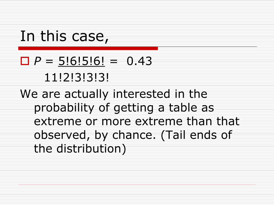
In this case,

P = 5!6!5!6! = 0.43

11!2!3!3!3!

We are actually interested in the probability of getting a table as extreme or more extreme than that observed, by chance. (Tail ends of the distribution)

More extreme tables..(Jack’s treatment is worse than observed)

Technique Bleeding stopped

Bleeding continued

Totals

New 1 4 5

Banding 4 2 6

Totals 5 6 11

Technique Bleeding stopped

Bleeding continued

Totals

New 0 5 5

Banding 5 1 6

Totals 5 6 11

More extreme tables..(New treatment is better than observed)

Technique Bleeding stopped

Bleeding continued

Totals

New 3 2 5

Banding 2 4 6

Totals 5 6 11

Technique Bleeding stopped

Bleeding continued

Totals

New 4 1 5

Banding 1 5 6

Totals 5 6 11

More extreme tables..(New treatment is better than observed)

Technique Bleeding stopped

Bleeding continued

Totals

New 5 0 5

Banding 0 6 6

Totals 5 6 11

Fisher Exact Test (Cont’d)

Probabilities associated with our five more “extreme” tables: p = 5!6!5!6! / 11!1!4!4!2!2! = 0.08 p = 5!6!5!6!/11!0!5!5!1! = 0.01 p = 5!6!5!6! = 0.32 11!3!2!2!4! p = 5!6!5!6! = 0.06 11!4!1!1!5! p = 5!6!5!6! = 0.002 11!5!0!0!6! Our total probability of obtaining a table as extreme

or more extreme than that observed assuming no difference in treatments is the following: 0.43 + 0.08 + 0.01 + 0.32 + 0.06 +0.002

Fisher Exact Test (Cont’d)

Do not need to compare to a distribution since this is an exact probability.

Procedure involves calculating the exact probability of table, then reducing smallest element by 1 until you reach zero, followed by calculating probability of all tables and adding them together. Keep row and column totals constant!.

Parametric versus non-parametric tests

We use the mean and standard deviation to describe a sample or a population that is normally distributed.

We should not use the mean and standard deviation to describe samples or populations that are not normally distributed.

ANOVA and the t-test use means and standard deviations (population parameters). The Chi-square test relies upon the Chi-squared distribution.

Non-parametric tests should be used when we cannot make assumptions about the shape of the underyling population distribution.

Ranks

Heights: 165cm, 155cm, 170cm 2 1 3

Principles of Ranking

Rank observations from lowest (smallest value) to highest (largest value).

Tied observations receive a rank equal to the average of the ranks they would have received had there not been a tie.

Try 52, 40, 74, 18, 40

Case Scenario #4

You have developed a continuing education program for practicing physicians designed to improve their management of type 2 diabetes. “Quality scores” are based on a number of variables, such as percent of patients achieving optimal HbA1C%, etc. Lower scores are associated with better care. The ideal score is 100. You wish to find out if scores for individual participants improve over time.

Case Scenario #4 Cont’dPhysician Baseline 6 months after

completing quality curriculum

Difference

1 150 150 0

2 160 170 -10

3 110 90 20

4 155 145 10

5 170 130 40

6 190 210 -20

7 160 160 0

8 180 150 30

9 145 170 -25

10 180 175 5

Wilcoxon Signed Rank Test

Frank Wilcoxon (1882 –1965)

Paired differences must be independent.

First rank all differences with respect to magnitude, ignoring their sign.

Zero differences are not ranked.

Tied differences receive the average of the rank they would have received had they not been tied.

Next we assign the sign of the difference to the ranks and simply add up these ranks.

Wilcoxon Signed Rank Test

Basic rationale:

“If the treatment did not have a significant effect, the magnitude of positive and negative ranks should be approximately the same, and the sum of the ranks should be close to zero.”

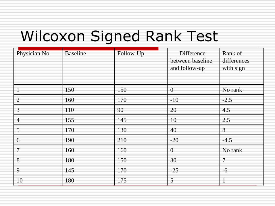
Wilcoxon Signed Rank TestPhysician No. Baseline Follow-Up Difference

between baseline

and follow-up

Rank of

differences

with sign

1 150 150 0 No rank

2 160 170 -10 -2.5

3 110 90 20 4.5

4 155 145 10 2.5

5 170 130 40 8

6 190 210 -20 -4.5

7 160 160 0 No rank

8 180 150 30 7

9 145 170 -25 -6

10 180 175 5 1

Wilcoxon Signed Rank(Cont’d)

Sum of ranks is the Wilcoxon statistic, W.

We compare our W to the values that would be obtained had there been no treatment effect.

μW = 0; σW =

ZW = |W| - ½

______________ 1)/6 1)(2n [n(n

1)/6 1)(2n [n(n

Correlation and Regression

Correlation is a statistical measure of the strength of association between two quantitative variables.

Association does not mean causality.

Regression used to identify relationships between one or more predictor variables upon an outcome variable.

Regression (Cont’d)

Simple linear regression

Logistic regression

Ordinal regression

Multiple regression

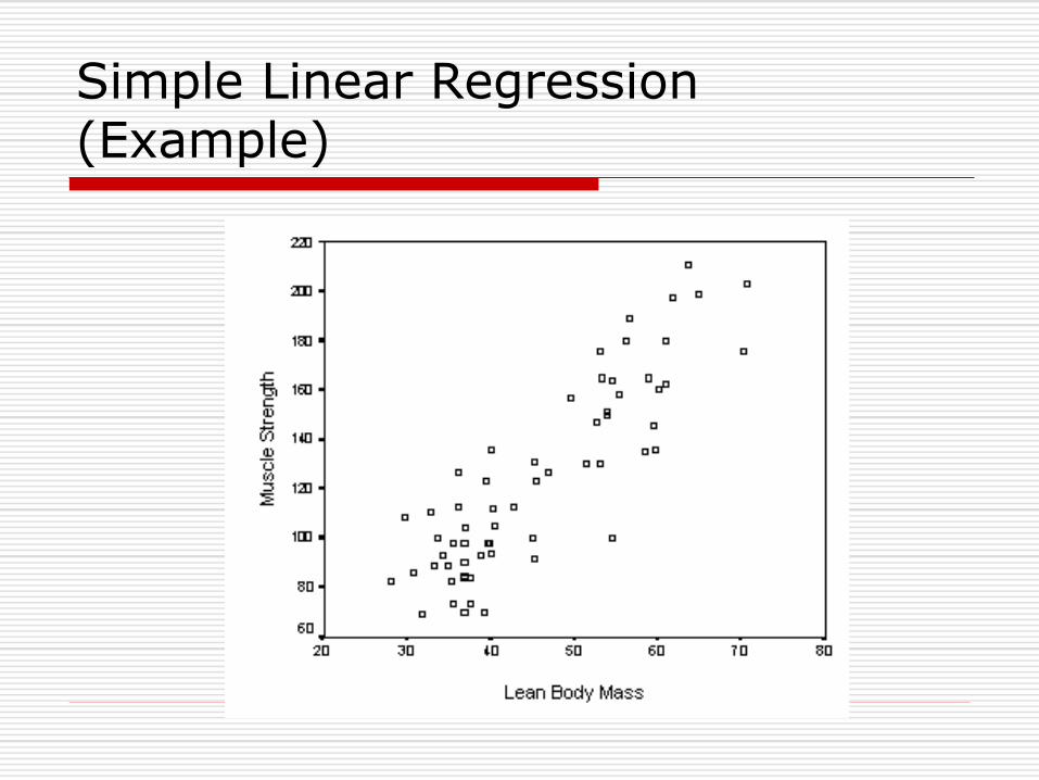
Simple Linear Regression (Example)

Simple Linear Regression

Sample Regression