64
030 295 7658 / 055 982 5292 | [email protected] | www.a-strategic.com Statistical Tools for Quantitative Research Part III Prof. Kafui Etsey University of Cape Coast

030 295 7658 / 055 982 5292 | [email protected] | www.a-strategic.com
Statistical Tools for Quantitative Research
Part III
Prof. Kafui Etsey
University of Cape Coast
[email protected] | 030 295 7658 / 055 982 5292
Prof. Kafui Etsey Statistical tools for Quantitative Research
[email protected] | 030 295 7658 / 055 982 5292
Introduction
Prof. Kafui Etsey Statistical tools for Quantitative Research

[email protected] | 030 295 7658 / 055 982 5292
Welcome Notes
o Welcome to today’s presentation, which is the third in the
series, on statistical tools for quantitative research.
o Webinars are always a learning situation in the face of rapid
changes in all spheres of life.
o I have been encouraged by the responses to the first and
second presentations.
o Godwilling, this will be our last presentation. Thank you all
for being part of this webinar.
Prof. Kafui Etsey Welcome Notes

[email protected] | 030 295 7658 / 055 982 5292
Prof. Kafui EtseyMain Focus of Webinar
Main Focus of the Webinar
o Describe the most commonly used tools in quantitative
research.
o Give examples of output and interpretations, where necessary.
o Challenge/motivate you to do more study on the tools, or seek
help.
o Most of the examples are in Education. You can apply it to your
areas of work if you are not in Education.
o Not involved in statistical computations or how the outcomes
are obtained.
[email protected] | 030 295 7658 / 055 982 5292
Statistical Inference
Prof. Kafui Etsey Statistical tools for Quantitative Research
[email protected] | 030 295 7658 / 055 982 5292
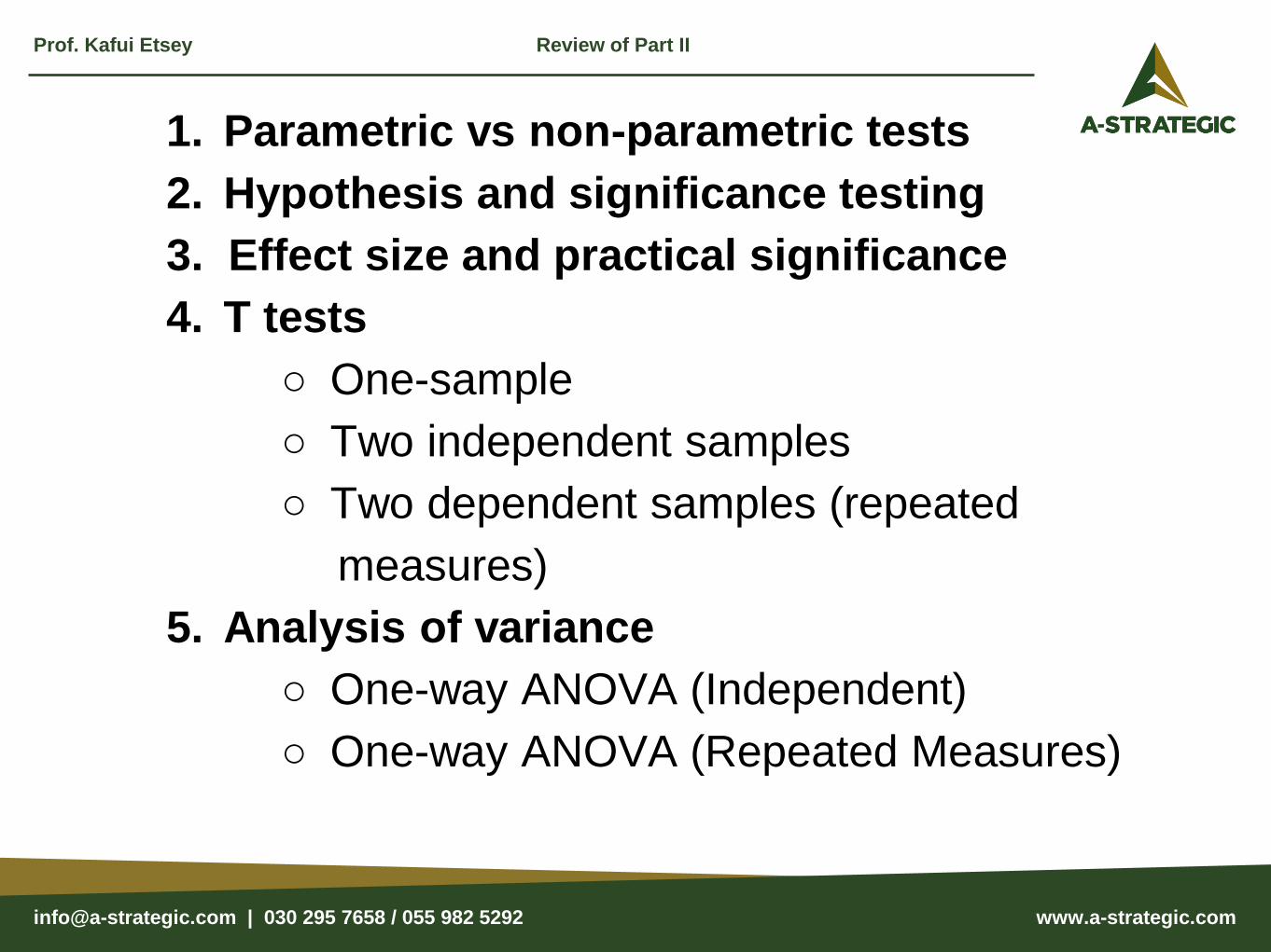
1. Parametric vs non-parametric tests
2. Hypothesis and significance testing
3. Effect size and practical significance
4. T tests
○ One-sample
○ Two independent samples
○ Two dependent samples (repeated
measures)
5. Analysis of variance
○ One-way ANOVA (Independent)
○ One-way ANOVA (Repeated Measures)
Prof. Kafui Etsey Review of Part II
[email protected] | 030 295 7658 / 055 982 5292
Prof. Kafui EtseyOverview
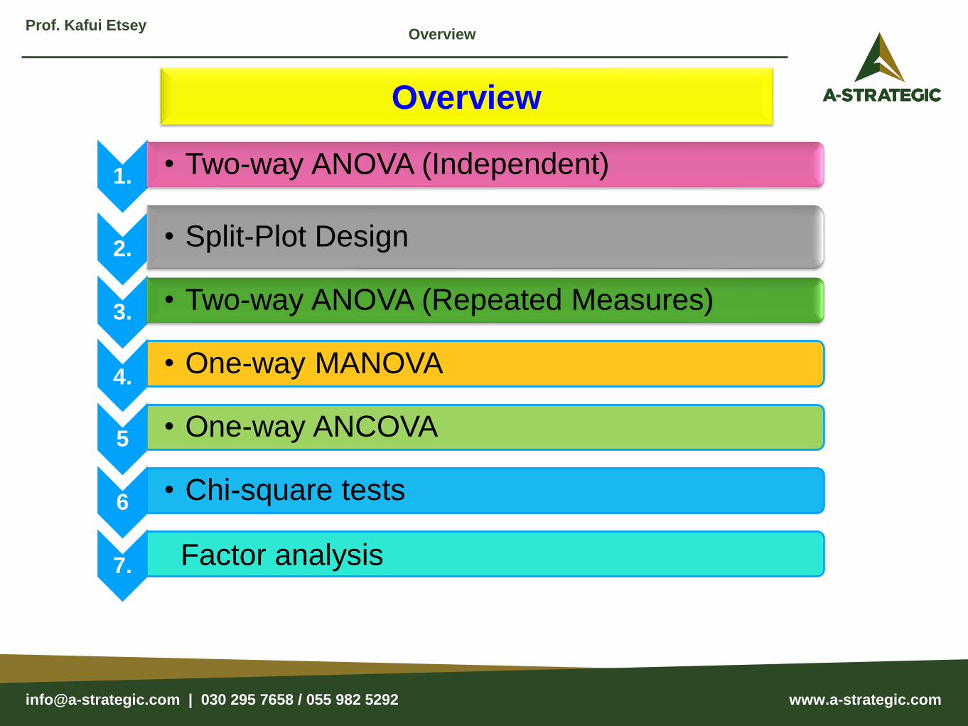
1. • Two-way ANOVA (Independent)
2. • Split-Plot Design
3. • Two-way ANOVA (Repeated Measures)
4.• One-way MANOVA
5 • One-way ANCOVA
6 • Chi-square tests
7. Factor analysis
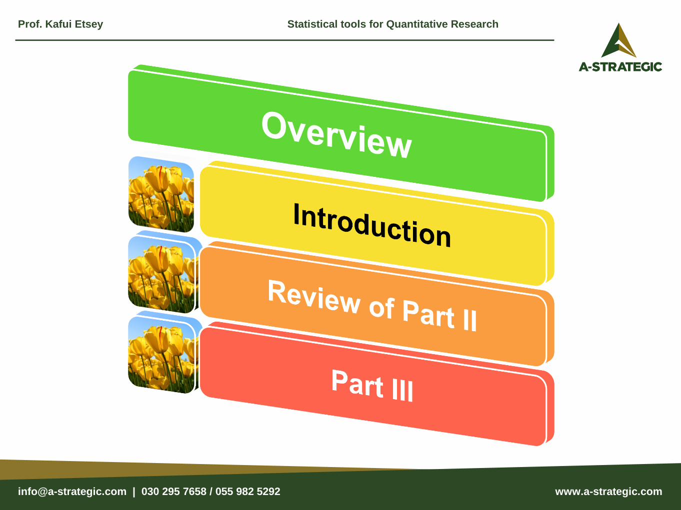
Overview
[email protected] | 030 295 7658 / 055 982 5292
Two Way ANOVA
(Independent)
Prof. Kafui EtseyTwo Way ANOVA
[email protected] | 030 295 7658 / 055 982 5292
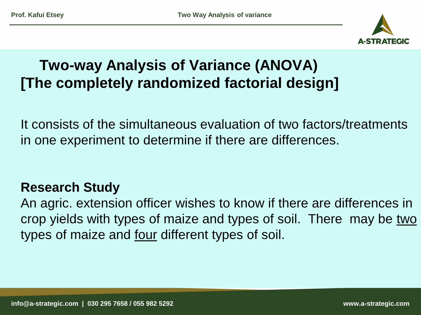
Two-way Analysis of Variance (ANOVA)
[The completely randomized factorial design]
It consists of the simultaneous evaluation of two factors/treatments
in one experiment to determine if there are differences.
Research Study
An agric. extension officer wishes to know if there are differences in
crop yields with types of maize and types of soil. There may be two
types of maize and four different types of soil.
Prof. Kafui Etsey Two Way Analysis of variance
[email protected] | 030 295 7658 / 055 982 5292
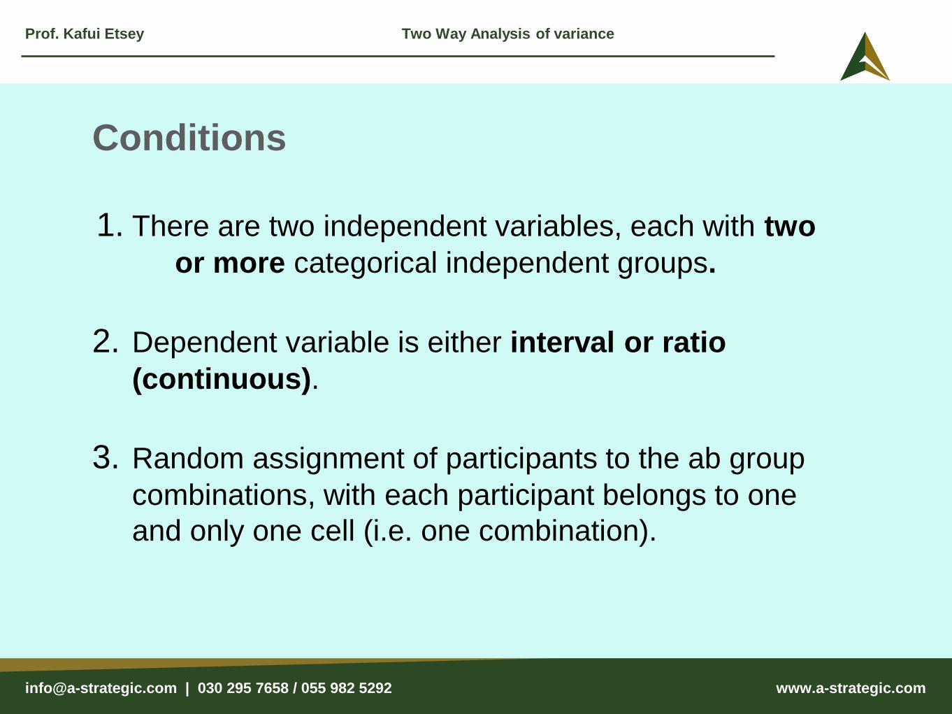
Conditions
1. There are two independent variables, each with two
or more categorical independent groups.
2. Dependent variable is either interval or ratio
(continuous).
3. Random assignment of participants to the ab group
combinations, with each participant belongs to one
and only one cell (i.e. one combination).
Prof. Kafui Etsey Two Way Analysis of variance
[email protected] | 030 295 7658 / 055 982 5292
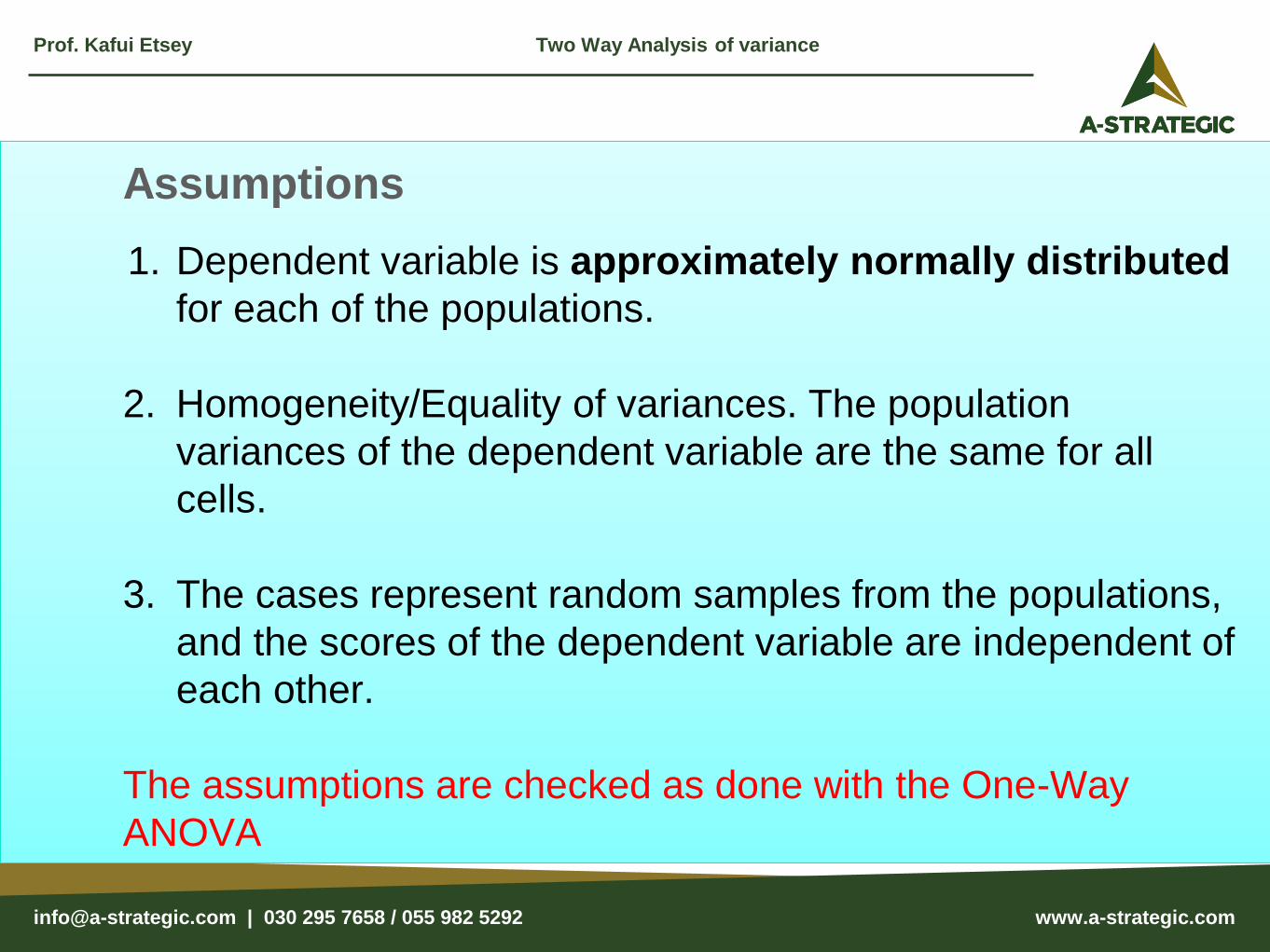
Assumptions
1. Dependent variable is approximately normally distributed
for each of the populations.
2. Homogeneity/Equality of variances. The population
variances of the dependent variable are the same for all
cells.
3. The cases represent random samples from the populations,
and the scores of the dependent variable are independent of
each other.
The assumptions are checked as done with the One-Way
ANOVA
Prof. Kafui Etsey Two Way Analysis of variance
[email protected] | 030 295 7658 / 055 982 5292
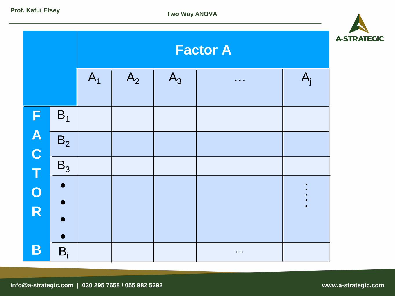
Prof. Kafui EtseyTwo Way ANOVA
Factor A
A1 A2 A3 … Aj
F
A
C
T
O
R
B
B1
B2
B3
•
•
•
•
•
•
•
•
•
Bi…
[email protected] | 030 295 7658 / 055 982 5292
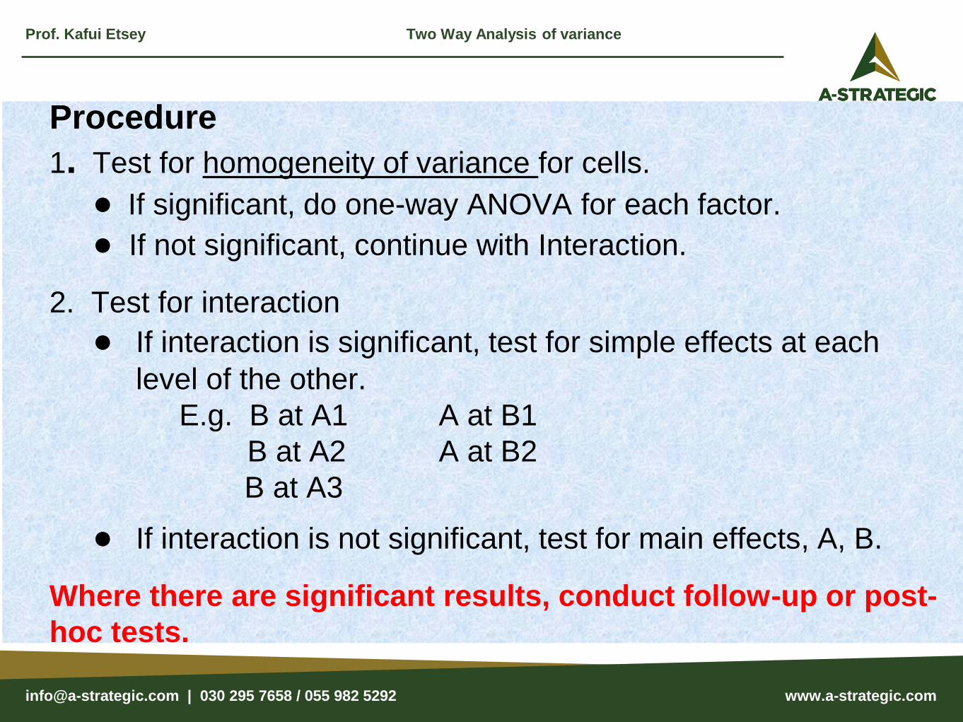
Procedure
1. Test for homogeneity of variance for cells.
● If significant, do one-way ANOVA for each factor.
● If not significant, continue with Interaction.
2. Test for interaction
● If interaction is significant, test for simple effects at each
level of the other.
E.g. B at A1 A at B1
B at A2 A at B2
B at A3
● If interaction is not significant, test for main effects, A, B.
Where there are significant results, conduct follow-up or post-
hoc tests.
Prof. Kafui Etsey Two Way Analysis of variance
[email protected] | 030 295 7658 / 055 982 5292
Split-Plot Design ANOVA
(Repeated Measures)
Prof. Kafui EtseySplit-Plot Design ANOVA
[email protected] | 030 295 7658 / 055 982 5292
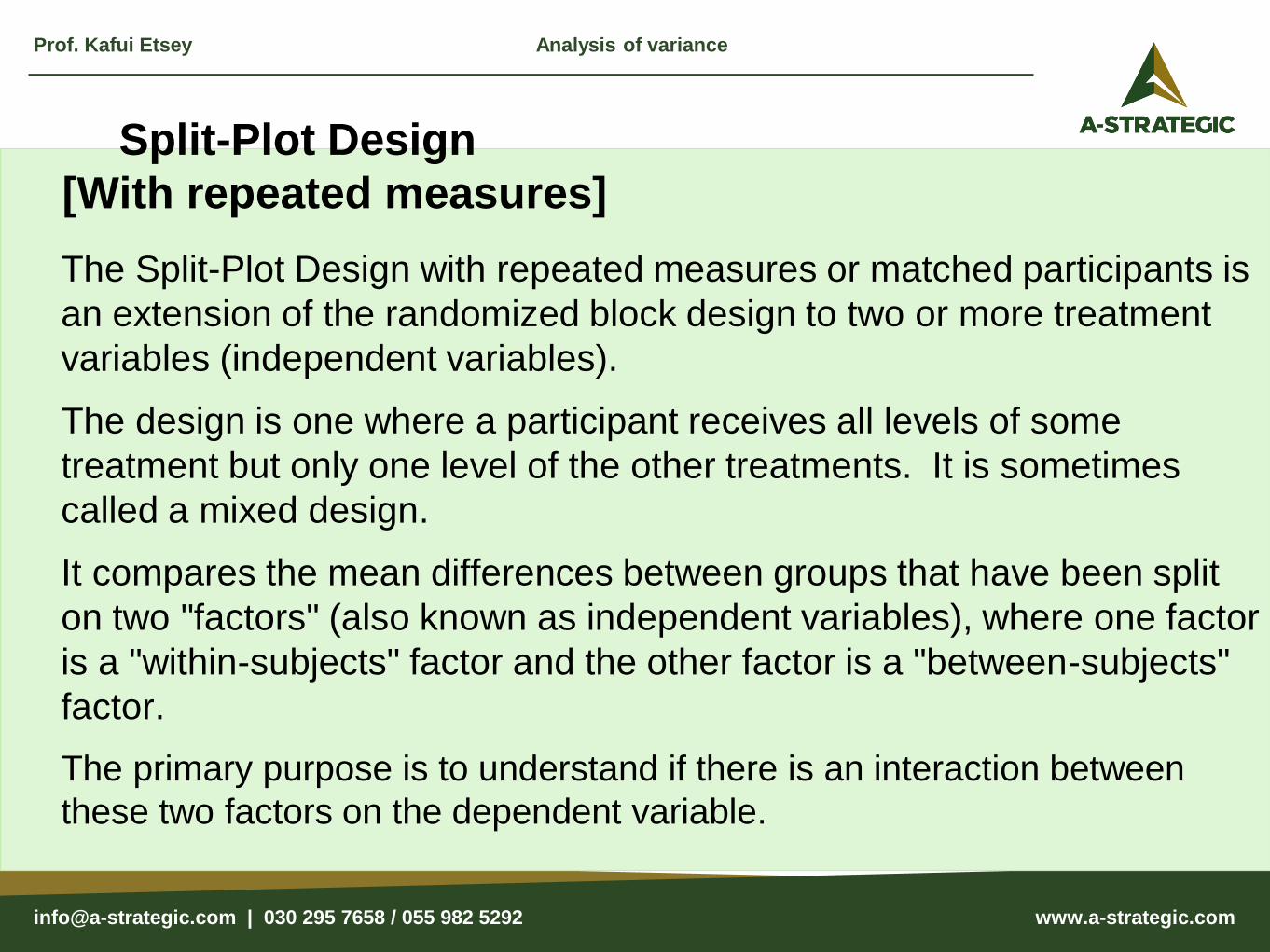
Split-Plot Design
[With repeated measures]
The Split-Plot Design with repeated measures or matched participants is
an extension of the randomized block design to two or more treatment
variables (independent variables).
The design is one where a participant receives all levels of some
treatment but only one level of the other treatments. It is sometimes
called a mixed design.
It compares the mean differences between groups that have been split
on two "factors" (also known as independent variables), where one factor
is a "within-subjects" factor and the other factor is a "between-subjects"
factor.
The primary purpose is to understand if there is an interaction between
these two factors on the dependent variable.
Prof. Kafui Etsey Analysis of variance
[email protected] | 030 295 7658 / 055 982 5292
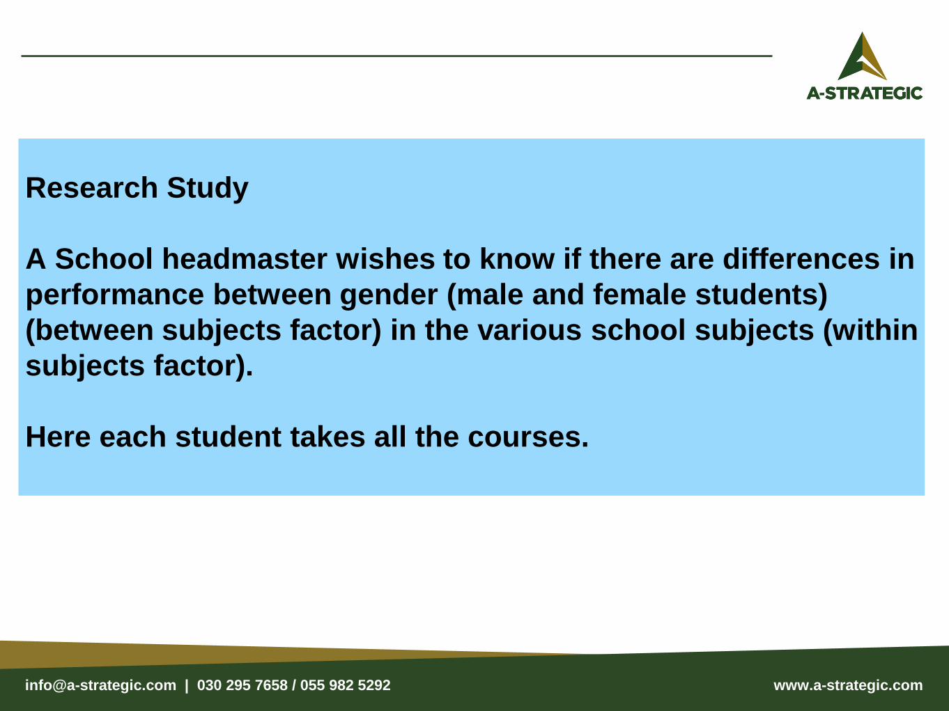
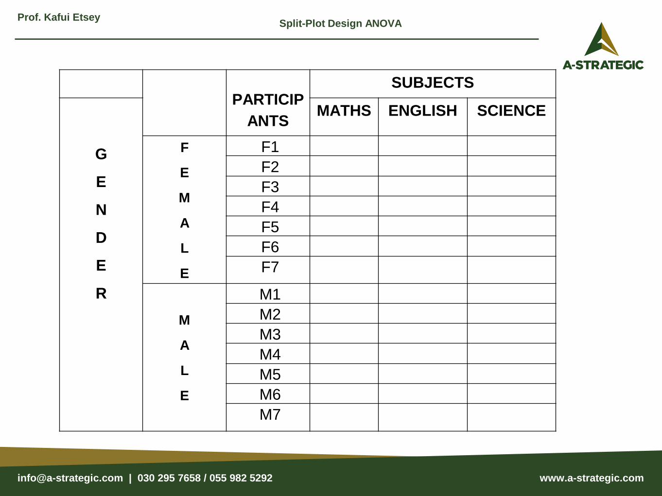
Research Study
A School headmaster wishes to know if there are differences in
performance between gender (male and female students)
(between subjects factor) in the various school subjects (within
subjects factor).
Here each student takes all the courses.
[email protected] | 030 295 7658 / 055 982 5292
Prof. Kafui EtseySplit-Plot Design ANOVA
PARTICIP
ANTS
SUBJECTS
G
E
N
D
E
R
MATHS ENGLISH SCIENCE
F
E
M
A
L
E
F1
F2
F3
F4
F5
F6
F7
M
A
L
E
M1
M2
M3
M4
M5
M6
M7
[email protected] | 030 295 7658 / 055 982 5292
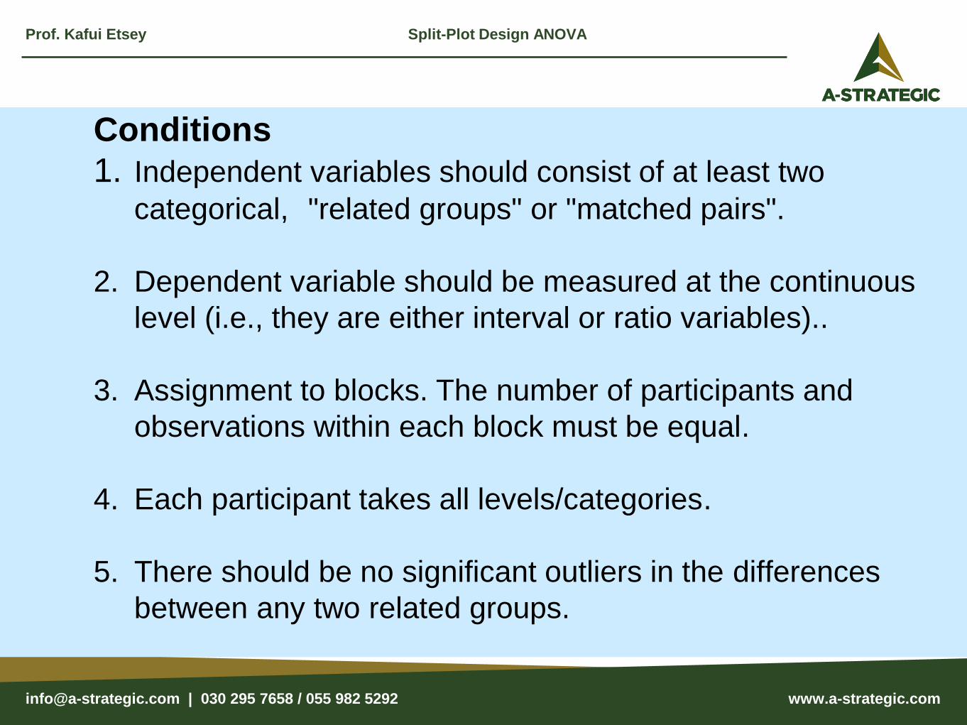
Conditions
1. Independent variables should consist of at least two
categorical, "related groups" or "matched pairs".
2. Dependent variable should be measured at the continuous
level (i.e., they are either interval or ratio variables)..
3. Assignment to blocks. The number of participants and
observations within each block must be equal.
4. Each participant takes all levels/categories.
5. There should be no significant outliers in the differences
between any two related groups.
Prof. Kafui Etsey Split-Plot Design ANOVA
[email protected] | 030 295 7658 / 055 982 5292
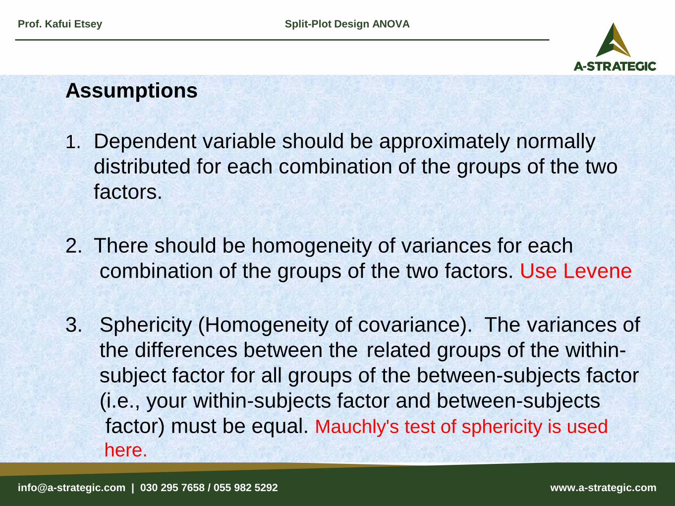
Assumptions
1. Dependent variable should be approximately normally
distributed for each combination of the groups of the two
factors.
2. There should be homogeneity of variances for each
combination of the groups of the two factors. Use Levene
3. Sphericity (Homogeneity of covariance). The variances of
the differences between the related groups of the within-
subject factor for all groups of the between-subjects factor
(i.e., your within-subjects factor and between-subjects
factor) must be equal. Mauchly's test of sphericity is used
here.
Prof. Kafui Etsey Split-Plot Design ANOVA
[email protected] | 030 295 7658 / 055 982 5292
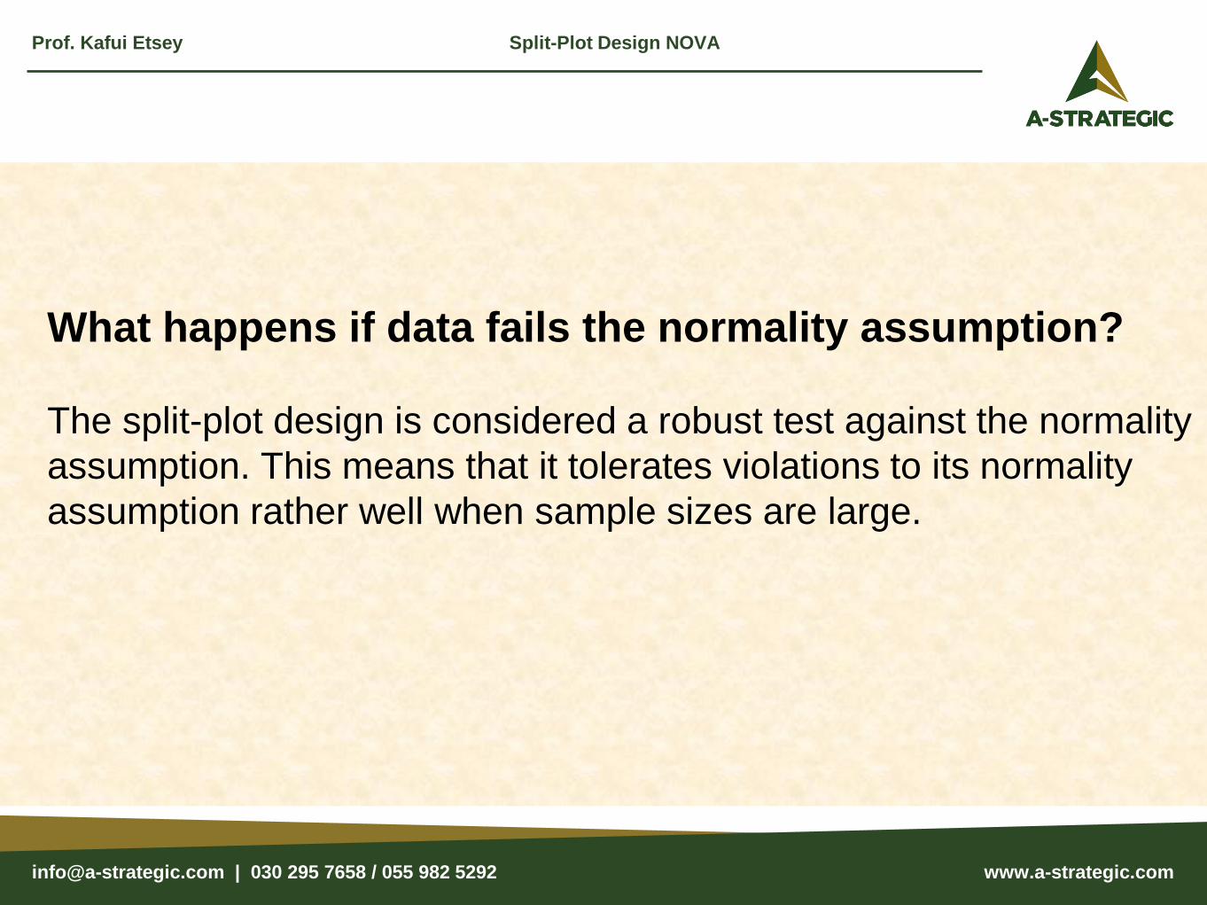
What happens if data fails the normality assumption?
The split-plot design is considered a robust test against the normality
assumption. This means that it tolerates violations to its normality
assumption rather well when sample sizes are large.
Prof. Kafui Etsey Split-Plot Design NOVA
[email protected] | 030 295 7658 / 055 982 5292
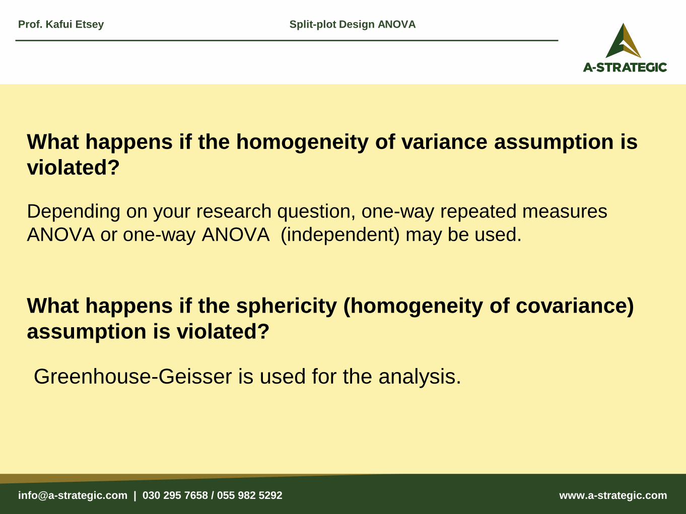
What happens if the homogeneity of variance assumption is
violated?
Depending on your research question, one-way repeated measures
ANOVA or one-way ANOVA (independent) may be used.
What happens if the sphericity (homogeneity of covariance)
assumption is violated?
Greenhouse-Geisser is used for the analysis.
Prof. Kafui Etsey Split-plot Design ANOVA

[email protected] | 030 295 7658 / 055 982 5292
Interpreting Output.
If you have a statistically significant interaction, you need to
determine the difference between your groups at each level of
each factor. You do this by analysing your data again to
determine what are known as simple main effects.
If you do not have a statistically significant interaction, you
need to interpret and report the main effects within the Tests of
Within-Subjects Effects
If the result is significant, conduct a Post Hoc using
Bonferroni, or Dependent t test to identify the differences.
Prof. Kafui Etsey Split-Plot Design ANOVA
[email protected] | 030 295 7658 / 055 982 5292
Two-way Repeated Measures ANOVA
Prof. Kafui EtseyTwo Way Repeated Measures
[email protected] | 030 295 7658 / 055 982 5292
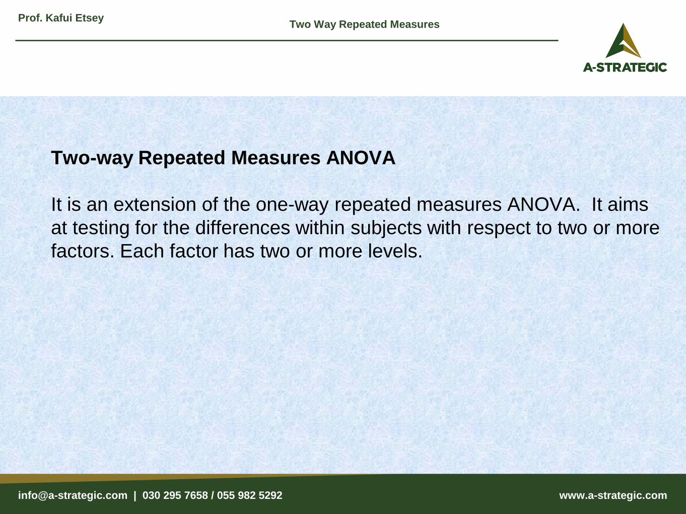
Two-way Repeated Measures ANOVA
It is an extension of the one-way repeated measures ANOVA. It aims
at testing for the differences within subjects with respect to two or more
factors. Each factor has two or more levels.
Prof. Kafui EtseyTwo Way Repeated Measures
[email protected] | 030 295 7658 / 055 982 5292
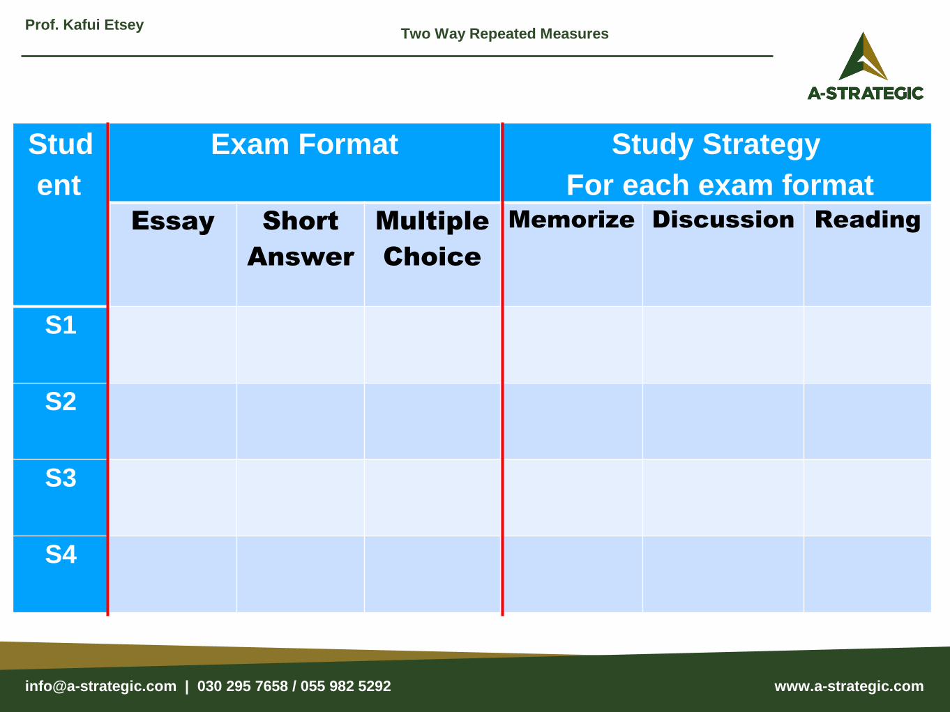
Prof. Kafui EtseyTwo Way Repeated Measures
Stud
ent
Exam Format Study Strategy
For each exam formatEssay Short
Answer
Multiple
Choice
Memorize Discussion Reading
S1
S2
S3
S4
[email protected] | 030 295 7658 / 055 982 5292
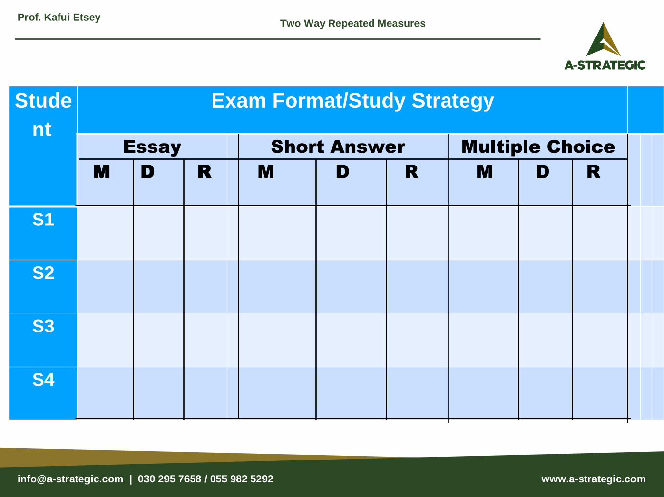
Prof. Kafui EtseyTwo Way Repeated Measures
Stude
nt
Exam Format/Study Strategy
Essay
M D R
Short Answer
M D R
Multiple Choice
M D R
S1
S2
S3
S4
[email protected] | 030 295 7658 / 055 982 5292
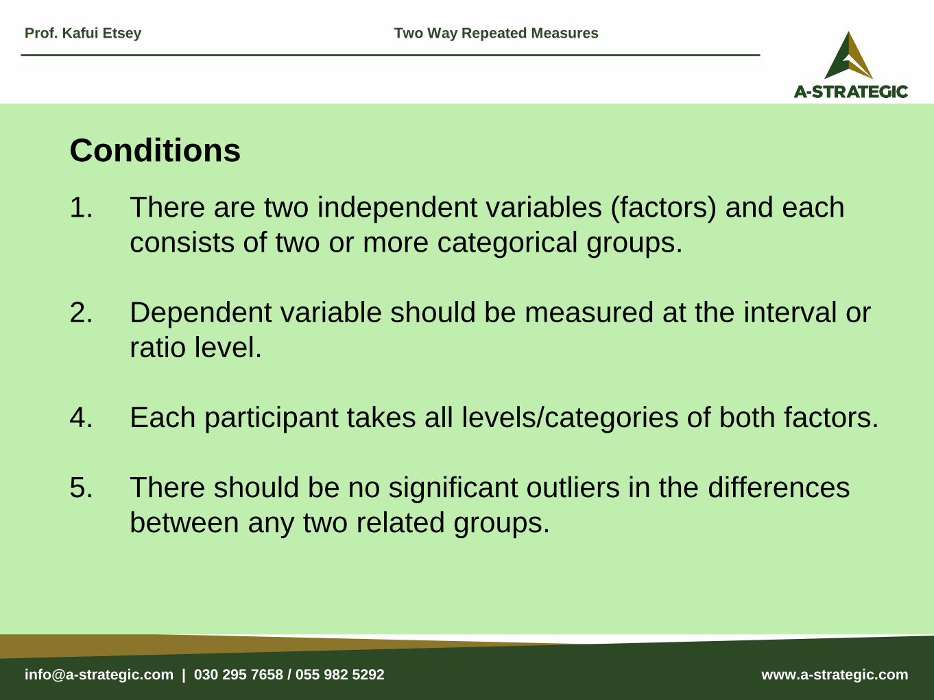
Conditions
1. There are two independent variables (factors) and each
consists of two or more categorical groups.
2. Dependent variable should be measured at the interval or
ratio level.
4. Each participant takes all levels/categories of both factors.
5. There should be no significant outliers in the differences
between any two related groups.
Prof. Kafui Etsey Two Way Repeated Measures
[email protected] | 030 295 7658 / 055 982 5292
Assumptions
1. The dependent variable is normally distributed in the
population for each combination of levels of the within-
subjects factors.
2. Sphericity. The variances of the differences between all
combinations of related groups must be equal.
The sphericity assumption is meaningful only if the main
effect or interaction effect has more than one degree of
freedom. If the assumption is violated, the p-value
associated with the standard univariate tests cannot be
trusted. The alternative univariate and multivariate
approaches are used.
3. The individuals represent a random sample from the
population and scores associated with different individuals
are not related.
Prof. Kafui Etsey Two Way Repeated Measures
[email protected] | 030 295 7658 / 055 982 5292
Approaches
1. There are three approaches for the test.
● Standard (traditional) univariate test. (This is used if the
main effect or interaction effect has a single degree of
freedom.
● Alternative (degrees-of-freedom corrected) univariate
test. This is used if the main effect or interaction effect
has more than a single degree of freedom. Does not
require sphericity.
● Multivariate test. This is used if the main effect or
interaction effect has more than a single degree of
freedom. Does not require sphericity.
In general, applied statisticians prefer the multivariate test.
Prof. Kafui Etsey Two Way Repeated Measures
[email protected] | 030 295 7658 / 055 982 5292
Procedure
1. Test for sphericity assumption
● If significant, do alternative univariate or multivariate test
or use Greenhouse Geisser.
● If not significant, continue with Interaction.
2. Test for interaction
● If interaction is significant, test for simple effects.
● If interaction is not significant, test for main effects.
Where there are significant results, conduct follow-up or post-
hoc tests.
Prof. Kafui Etsey Two Way Repeated Measures

[email protected] | 030 295 7658 / 055 982 5292
One-Way Multivariate Analysis of
Variance (MANOVA)
Prof. Kafui EtseyOne Way MANOVA
[email protected] | 030 295 7658 / 055 982 5292
ONE-WAY MANOVA
The main purpose is to evaluate whether population means on a set
of dependent variables vary across levels of a factor or factors. It is
a techniques of determining whether groups differ on more than one
dependent variable. It also evaluates equality among groups on
linear combinations of dependent variables
The independent variables are factors that have two or more levels
with multiple dependent variables and not a single dependent
variable as in ANOVA.
Each research participant has a score on two or more dependent
variables.
Prof. Kafui Etsey One Way MANOVA
[email protected] | 030 295 7658 / 055 982 5292
ONE-WAY MANOVA
Eg. A study to examine the effects of study strategies on
learning.
Study strategies include memorization, writing and exposition.
Final quiz, the dependent variable, includes questions on
knowledge, comprehension and application.
Are the population means for the scores on knowledge,
comprehension and application the same or different for
students in the three study groups?
Or is there a relationship between type of study strategy and
performance on test items (knowledge, comprehension,
application)?
Prof. Kafui Etsey One Way MANOVA
[email protected] | 030 295 7658 / 055 982 5292
Conditions
1. There are two independent variables (factors) and each
consists of two or more categorical groups.
2. There are two or more dependent variables each
measured at the interval or ratio level.
5. There should be no significant outliers in the differences
between any two related groups.
Prof. Kafui Etsey One Way MANOVA
[email protected] | 030 295 7658 / 055 982 5292
Assumptions
1. The dependent variables are multivariately normally
distributed for each population with the different
populations being defined by the levels of the Factor.
2. The population variances and covariances among the
dependent variables are the same across all levels of the
Factor.
3. The participants are randomly sampled from the
population and scores associated with different
individuals are independent.
Prof. Kafui Etsey One Way MANOVA
[email protected] | 030 295 7658 / 055 982 5292
Prof. Kafui EtseyOne Way MANOVA
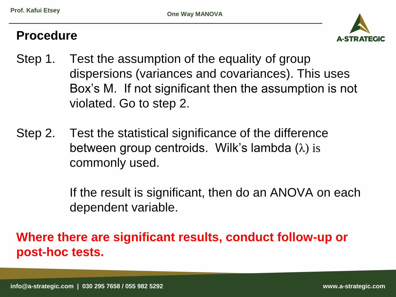
Procedure
Step 1. Test the assumption of the equality of group
dispersions (variances and covariances). This uses
Box’s M. If not significant then the assumption is not
violated. Go to step 2.
Step 2. Test the statistical significance of the difference
between group centroids. Wilk’s lambda (λ) is
commonly used.
If the result is significant, then do an ANOVA on each
dependent variable.
Where there are significant results, conduct follow-up or
post-hoc tests.
[email protected] | 030 295 7658 / 055 982 5292
One-Way Analysis of Covariance
(ANCOVA)
Prof. Kafui EtseyOne Way ANCOVA
[email protected] | 030 295 7658 / 055 982 5292
One-Way Analysis of Covariance (ANCOVA)
The main purpose is to evaluate differences among groups with
respect to a dependent variable, adjusting for initial differences on
the covariate.
It is used to control for initial differences between groups before a
comparison of the within-groups variance and between groups
variance is made.
The effect of ANCOVA is to make the groups equal with respect to
one or more control variables.
Prof. Kafui Etsey One Way ANCOVA
[email protected] | 030 295 7658 / 055 982 5292
It used to:
○ Increase statistical power
○ Reduce bias by equating statistically groups on one or
more variables
E.g. A study to find out the differences in performance in
Mathematics in three schools ( A, B, C, classification).
The classification may be based on resources in the schools.
The resources would be used as a covariate to adjust the scores
before the analysis is done using ANCOVA.
Prof. Kafui Etsey One Way ANCOVA
[email protected] | 030 295 7658 / 055 982 5292
Assumptions
1. The dependent variable is normally distributed in the
population for any specific value of the covariate and for
any one level of a factor.
2. The variances of the dependent variable for the conditional
distributions as in (1) above are equal.
3. Scores on the dependent variable are independent of each
other.
4. Covariate is fixed and contains no measurement error.
Prof. Kafui Etsey One Way ANCOVA
[email protected] | 030 295 7658 / 055 982 5292
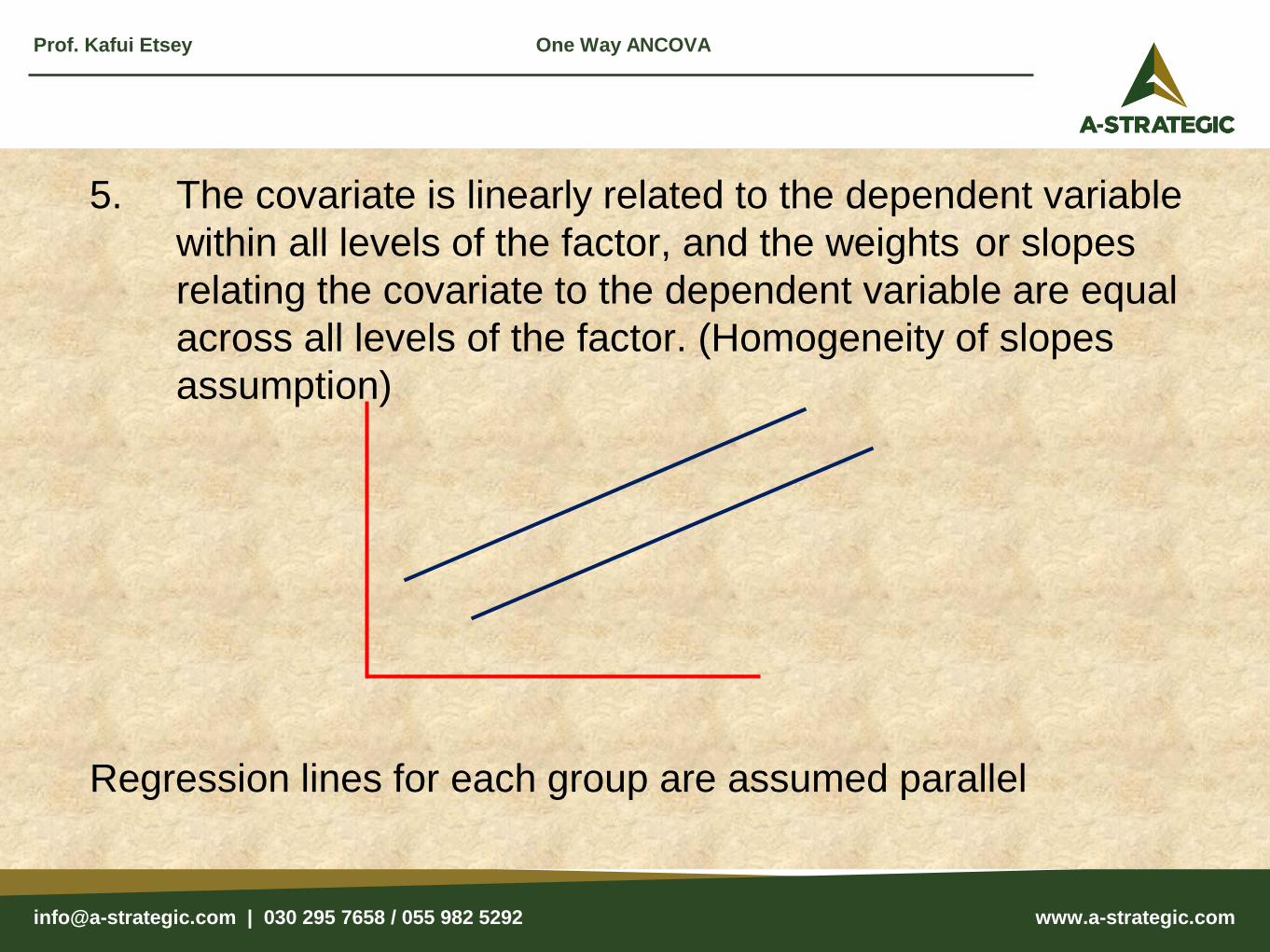
5. The covariate is linearly related to the dependent variable
within all levels of the factor, and the weights or slopes
relating the covariate to the dependent variable are equal
across all levels of the factor. (Homogeneity of slopes
assumption)
Regression lines for each group are assumed parallel
Prof. Kafui Etsey One Way ANCOVA
[email protected] | 030 295 7658 / 055 982 5292
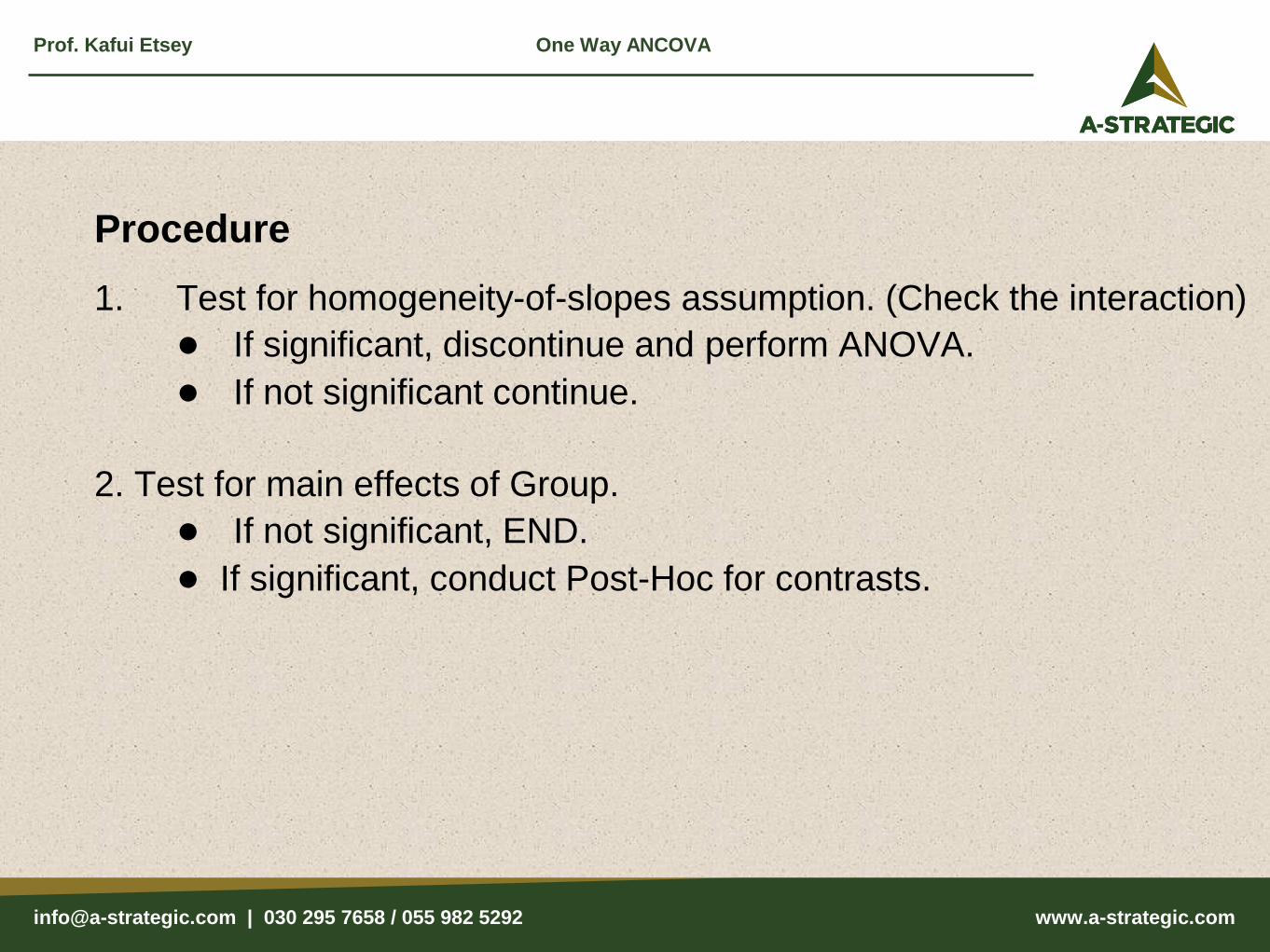
Procedure
1. Test for homogeneity-of-slopes assumption. (Check the interaction)
● If significant, discontinue and perform ANOVA.
● If not significant continue.
2. Test for main effects of Group.
● If not significant, END.
● If significant, conduct Post-Hoc for contrasts.
Prof. Kafui Etsey One Way ANCOVA
[email protected] | 030 295 7658 / 055 982 5292
There are two main Chi-Square ( ) Tests
1. Test of goodness of fit
2. Test of independence/association
However the test of independence/association is
most widely used in research
Prof. Kafui EtseyChi-square
[email protected] | 030 295 7658 / 055 982 5292
The chi-squared test is used mostly to find the association
between two nominal variables. It deals with relationships
between variables.
It determines whether two nominal variables are related or
independent of each other. Each variable has two or more
categories.
It is a non-parametric test.
Contingency tables are produced as the initial output.
Contingency tables are described in terms of number of rows
and number of columns as r x c
Prof. Kafui EtseyChi-square
[email protected] | 030 295 7658 / 055 982 5292
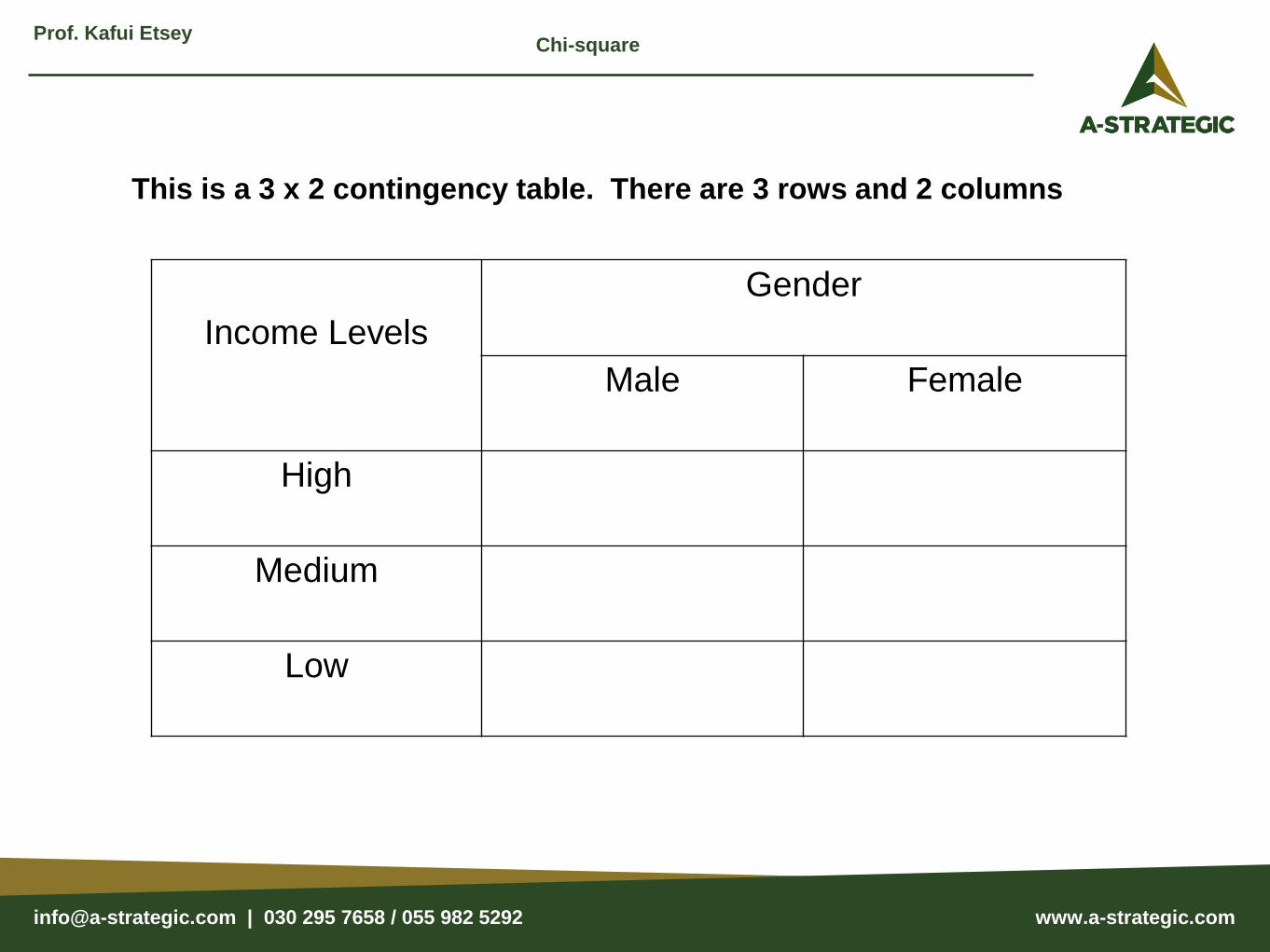
Prof. Kafui EtseyChi-square
Income Levels
Gender
Male Female
High
Medium
Low
This is a 3 x 2 contingency table. There are 3 rows and 2 columns

[email protected] | 030 295 7658 / 055 982 5292
Research Studies
1. A researcher may want to know if there is an
association between gender (male, female) and
courses offered ( Arts, Business, Science) in an
institution.
2. An executive director of a company may want to know
if there is an association between educational
level/attainment (Senior High, First degree and Higher
degree) and job rating (Excellent, Good and Fair).
Prof. Kafui EtseyChi-square
[email protected] | 030 295 7658 / 055 982 5292
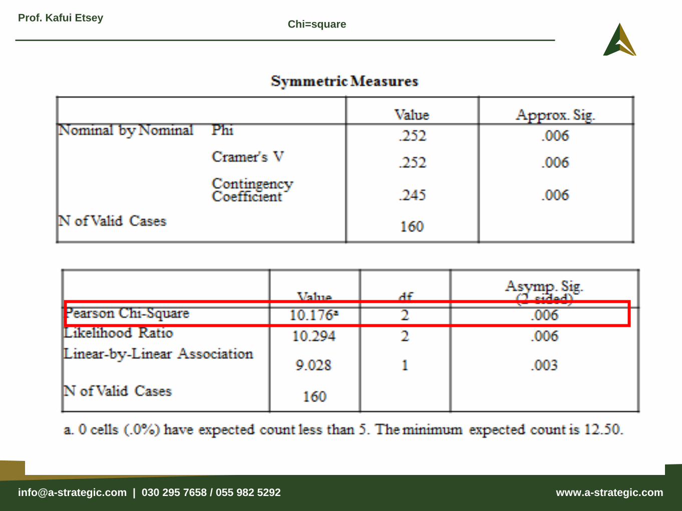
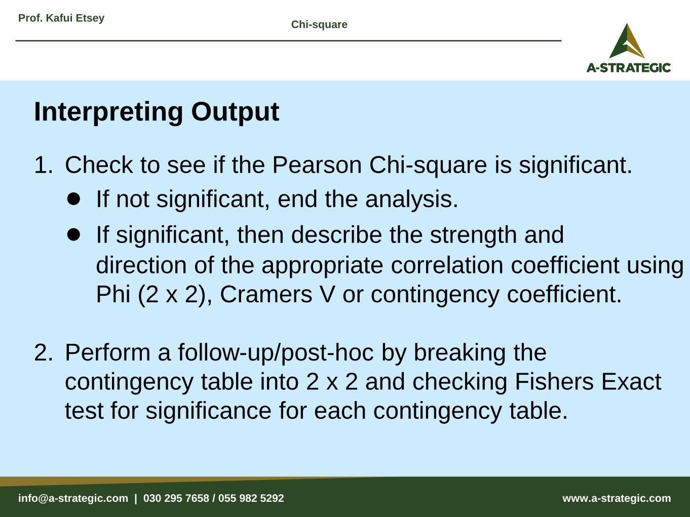
Interpreting Output
1. Check to see if the Pearson Chi-square is significant.
● If not significant, end the analysis.
● If significant, then describe the strength and
direction of the appropriate correlation coefficient using
Phi (2 x 2), Cramers V or contingency coefficient.
2. Perform a follow-up/post-hoc by breaking the
contingency table into 2 x 2 and checking Fishers Exact
test for significance for each contingency table.
Prof. Kafui EtseyChi-square
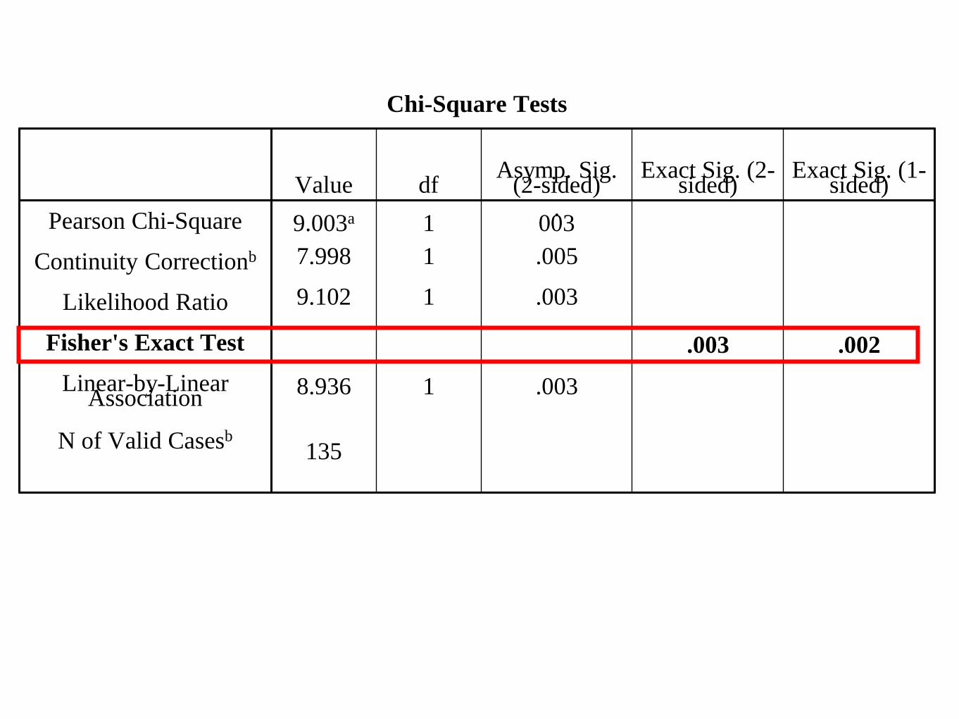
Chi-Square Tests
Value dfAsymp. Sig.
(2-sided)Exact Sig. (2-
sided)Exact Sig. (1-
sided)
Pearson Chi-Square 9.003a 1.
003
Continuity Correctionb 7.998 1 .005
Likelihood Ratio 9.102 1 .003
Fisher's Exact Test .003 .002
Linear-by-Linear Association
8.936 1 .003
N of Valid Casesb135
[email protected] | 030 295 7658 / 055 982 5292
Prof. Kafui EtseyChi-square
Loglinear analysis
It is an extension of the Chi-square tests. It uses nominal data.
It is used to determine if there is a significant relationship among
three or more categorical variables where each variable has a
number of levels.
It uses logs to transform categorical data into linear models.
For example, a relationship among gender (2 levels),
education (3 levels), and driving license type (3 levels) with
respect to number of road accidents in a city.
[email protected] | 030 295 7658 / 055 982 5292
Prof. Kafui EtseyFactor analysis
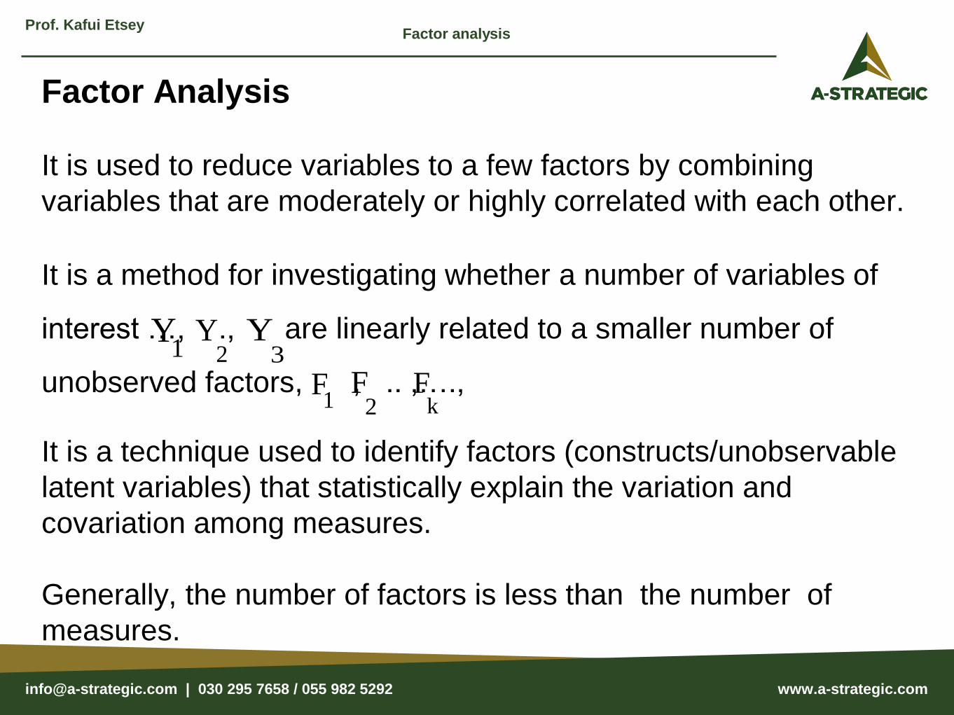
Factor Analysis
It is used to reduce variables to a few factors by combining
variables that are moderately or highly correlated with each other.
It is a method for investigating whether a number of variables of
interest …, ., are linearly related to a smaller number of
unobserved factors, , .. ,….,
It is a technique used to identify factors (constructs/unobservable
latent variables) that statistically explain the variation and
covariation among measures.
Generally, the number of factors is less than the number of
measures.
1Y
2Y
3Y
1F
2F
kF
[email protected] | 030 295 7658 / 055 982 5292
Prof. Kafui EtseyFactor analysis
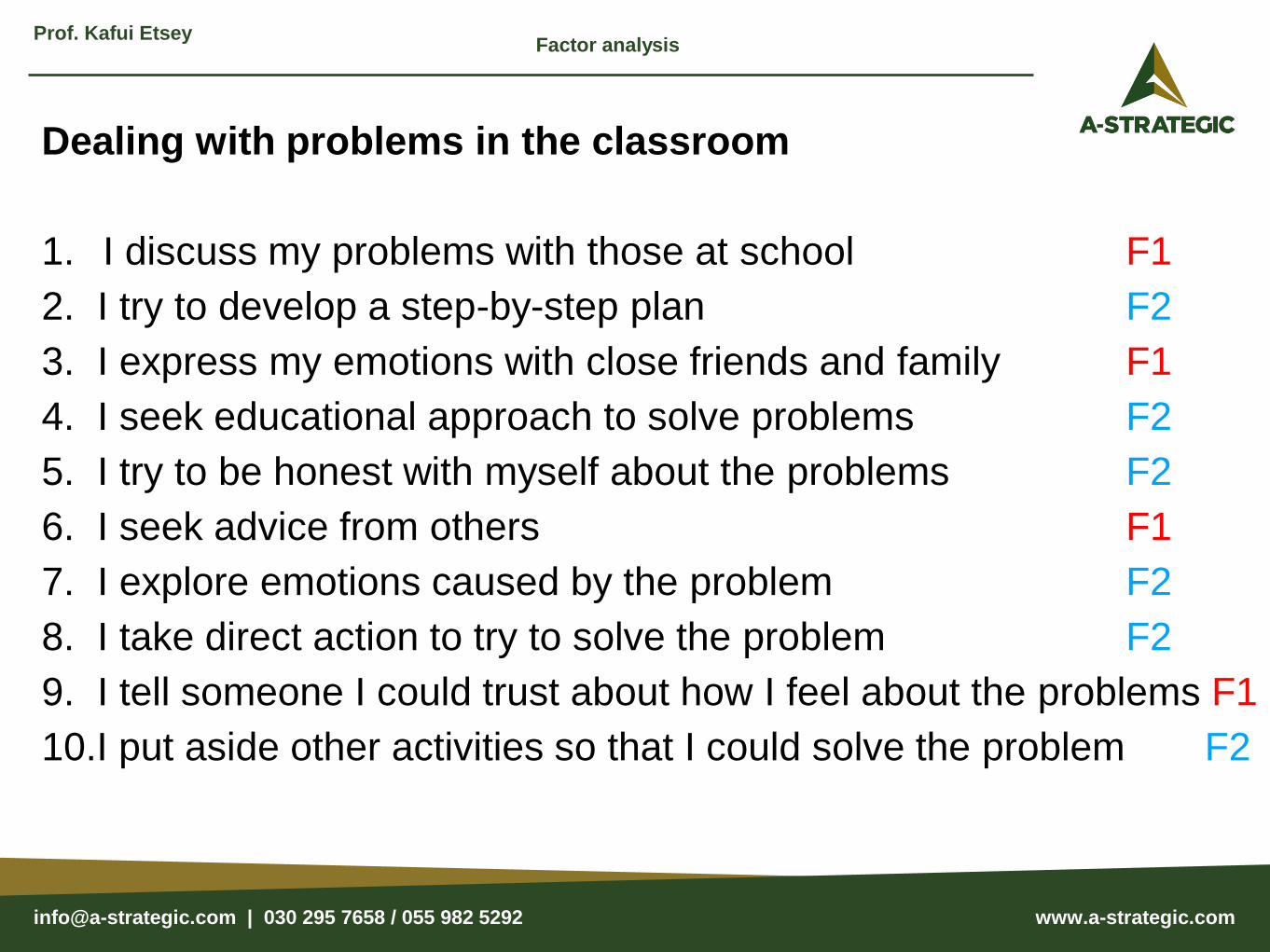
Dealing with problems in the classroom
1. I discuss my problems with those at school F1
2. I try to develop a step-by-step plan F2
3. I express my emotions with close friends and family F1
4. I seek educational approach to solve problems F2
5. I try to be honest with myself about the problems F2
6. I seek advice from others F1
7. I explore emotions caused by the problem F2
8. I take direct action to try to solve the problem F2
9. I tell someone I could trust about how I feel about the problems F1
10.I put aside other activities so that I could solve the problem F2
[email protected] | 030 295 7658 / 055 982 5292
Prof. Kafui EtseyFactor analysis
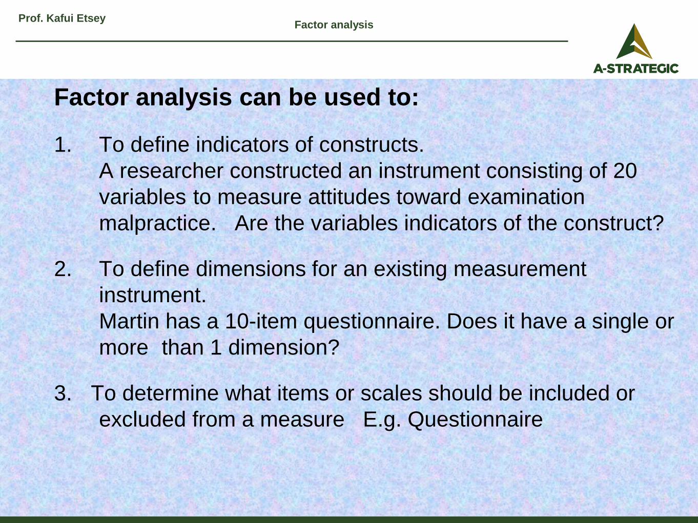
Factor analysis can be used to:
1. To define indicators of constructs.
A researcher constructed an instrument consisting of 20
variables to measure attitudes toward examination
malpractice. Are the variables indicators of the construct?
2. To define dimensions for an existing measurement
instrument.
Martin has a 10-item questionnaire. Does it have a single or
more than 1 dimension?
3. To determine what items or scales should be included or
excluded from a measure E.g. Questionnaire
[email protected] | 030 295 7658 / 055 982 5292
Prof. Kafui EtseyFactor Analysis
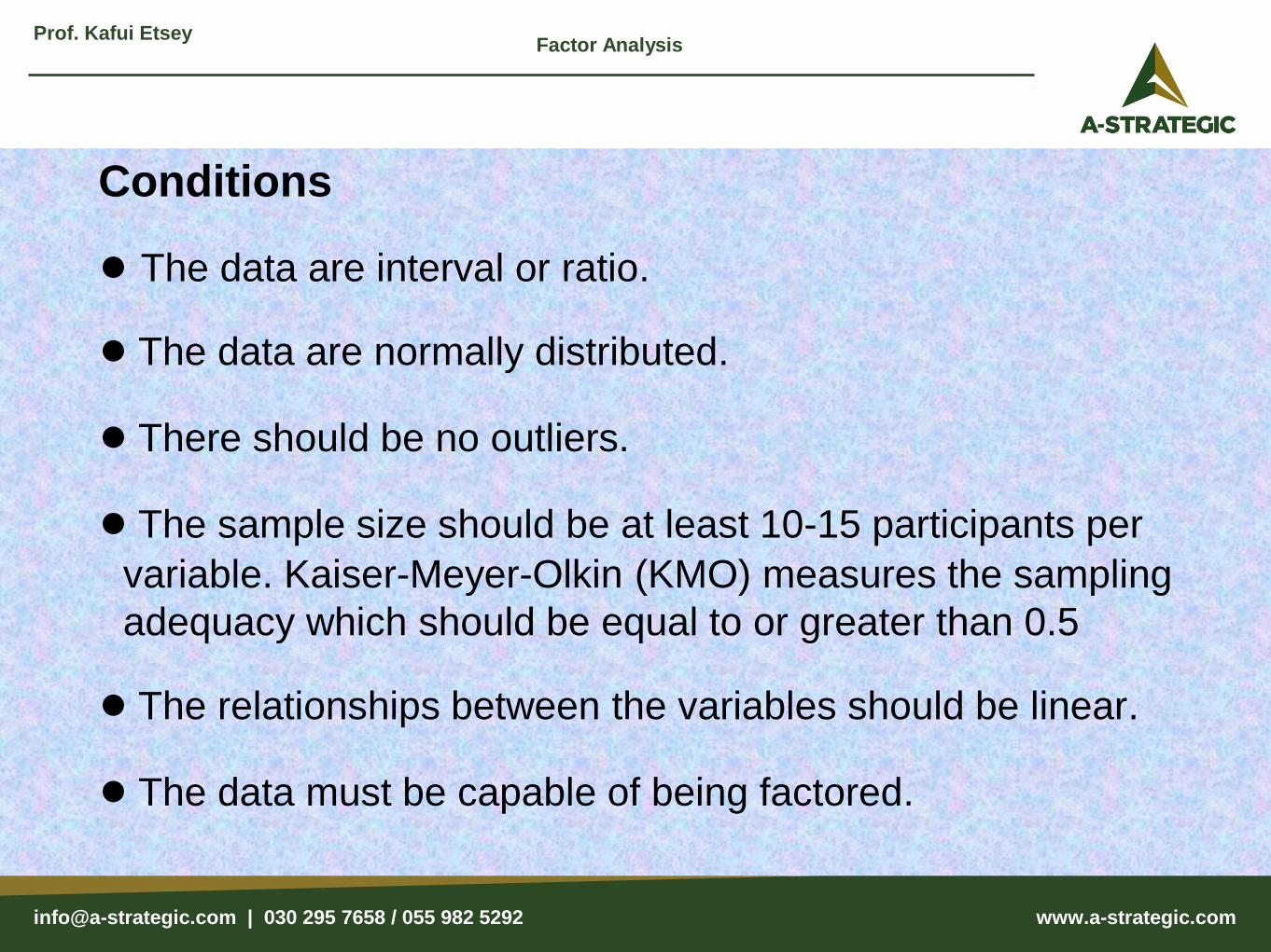
Conditions
● The data are interval or ratio.
● The data are normally distributed.
● There should be no outliers.
● The sample size should be at least 10-15 participants per
variable. Kaiser-Meyer-Olkin (KMO) measures the sampling
adequacy which should be equal to or greater than 0.5
● The relationships between the variables should be linear.
● The data must be capable of being factored.
[email protected] | 030 295 7658 / 055 982 5292
Prof. Kafui EtseyFactor Analysis
Assumptions
● Measured variables are linearly related to the factors.
Violated if: Items have limited responses (eg 2-point
responses, Yes/No)
● Errors are independent of each other.
● The unobservable factors are independent of each other.
● The unobservable factors are independent of the errors.
● Sphericity. The correlation matrix is an identity matrix, in which
all of the diagonal elements are 1 and all off diagonal elements
are 0. Bartlett’s test pf sphericity is done and must be
significant.
[email protected] | 030 295 7658 / 055 982 5292
Prof. Kafui EtseyFactor Analysis
Types
Exploratory
It is exploratory when you do not have a pre defined idea of the
structure or how many dimensions are in a set of variables.
Confirmatory
It is confirmatory when you want to test specific hypothesis about
the structure or the number of dimensions underlying a set of
variables (i.e. in your data you may think there are two
dimensions and you want to verify that)
[email protected] | 030 295 7658 / 055 982 5292
Prof. Kafui EtseyFctor Analysis
Main Stages
There are two main stages.
1. Factor Extraction
2. Factor Rotation
Factor Extraction
The objective is to make an initial decision about the number of
factors underlying a set of measured variables.
The main methods are the use of Eigen values and Scree test.
[email protected] | 030 295 7658 / 055 982 5292
Prof. Kafui EtseyFactor analysis
Factor Rotation
The objective is to make the factors interpretable and
meaningful.
It produces a table which contains the rotated factor
loadings , which represent both how the variables are
weighted for each factor and also the correlation
between the variables and the factor.
The factors are identified by the variables and labelled
(named) where appropriate.
[email protected] | 030 295 7658 / 055 982 5292
The End
Thanks for your cooperation
Prof. Kafui Etsey The End