51
STATISTICS FOR ECONOMISTS: A BEGINNING John E. Floyd University of Toronto July 2, 2010
STATISTICS FOR ECONOMISTS:
A BEGINNING
John E. FloydUniversity of Toronto
July 2, 2010
PREFACE
The pages that follow contain the material presented in my introductoryquantitative methods in economics class at the University of Toronto. Theyare designed to be used along with any reasonable statistics textbook. Themost recent textbook for the course was James T. McClave, P. George Ben-son and Terry Sincich, Statistics for Business and Economics, Eighth Edi-tion, Prentice Hall, 2001. The material draws upon earlier editions of thatbook as well as upon John Neter, William Wasserman and G. A. Whitmore,Applied Statistics, Fourth Edition, Allyn and Bacon, 1993, which was usedpreviously and is now out of print. It is also consistent with Gerald Kellerand Brian Warrack, Statistics for Management and Economics, Fifth Edi-tion, Duxbury, 2000, which is the textbook used recently on the St. GeorgeCampus of the University of Toronto. The problems at the ends of the chap-ters are questions from mid-term and final exams at both the St. Georgeand Mississauga campuses of the University of Toronto. They were set byGordon Anderson, Lee Bailey, Greg Jump, Victor Yu and others includingmyself.
This manuscript should be useful for economics and business students en-rolled in basic courses in statistics and, as well, for people who have studiedstatistics some time ago and need a review of what they are supposed to havelearned. Indeed, one could learn statistics from scratch using this materialalone, although those trying to do so may find the presentation somewhatcompact, requiring slow and careful reading and thought as one goes along.
I would like to thank the above mentioned colleagues and, in addition, Ado-nis Yatchew, for helpful discussions over the years, and John Maheu forhelping me clarify a number of points. I would especially like to thank Gor-don Anderson, who I have bothered so frequently with questions that hedeserves the status of mentor.
After the original version of this manuscript was completed, I received somedetailed comments on Chapter 8 from Peter Westfall of Texas Tech Univer-sity, enabling me to correct a number of errors. Such comments are muchappreciated.
J. E. FloydJuly 2, 2010
c⃝J. E. Floyd, University of Toronto
i

ii
Contents
1 Introduction to Statistics, Data and Statistical Thinking 1
1.1 What is Statistics? . . . . . . . . . . . . . . . . . . . . . . . . 1
1.2 The Use of Statistics in Economics and Other Social Sciences 1
1.3 Descriptive and Inferential Statistics . . . . . . . . . . . . . . 4
1.4 A Quick Glimpse at Statistical Inference . . . . . . . . . . . . 5
1.5 Data Sets . . . . . . . . . . . . . . . . . . . . . . . . . . . . . 7
1.6 Numerical Measures of Position . . . . . . . . . . . . . . . . . 18
1.7 Numerical Measures of Variability . . . . . . . . . . . . . . . 22
1.8 Numerical Measures of Skewness . . . . . . . . . . . . . . . . 24
1.9 Numerical Measures of Relative Position:Standardised Values . . . . . . . . . . . . . . . . . . . . . . . 25
1.10 Bivariate Data: Covariance and Correlation . . . . . . . . . . 27
1.11 Exercises . . . . . . . . . . . . . . . . . . . . . . . . . . . . . 31
2 Probability 35
2.1 Why Probability? . . . . . . . . . . . . . . . . . . . . . . . . . 35
2.2 Sample Spaces and Events . . . . . . . . . . . . . . . . . . . . 36
2.3 Univariate, Bivariate and Multivariate Sample Spaces . . . . 38
2.4 The Meaning of Probability . . . . . . . . . . . . . . . . . . . 40
2.5 Probability Assignment . . . . . . . . . . . . . . . . . . . . . 41
2.6 Probability Assignment in Bivariate Sample Spaces . . . . . . 44
2.7 Conditional Probability . . . . . . . . . . . . . . . . . . . . . 45
2.8 Statistical Independence . . . . . . . . . . . . . . . . . . . . . 46
2.9 Bayes Theorem . . . . . . . . . . . . . . . . . . . . . . . . . . 49
2.10 The AIDS Test . . . . . . . . . . . . . . . . . . . . . . . . . . 52
2.11 Basic Probability Theorems . . . . . . . . . . . . . . . . . . . 54
2.12 Exercises . . . . . . . . . . . . . . . . . . . . . . . . . . . . . 55
iii
3 Some Common Probability Distributions 63
3.1 Random Variables . . . . . . . . . . . . . . . . . . . . . . . . 63
3.2 Probability Distributions of Random Variables . . . . . . . . 64
3.3 Expected Value and Variance . . . . . . . . . . . . . . . . . . 67
3.4 Covariance and Correlation . . . . . . . . . . . . . . . . . . . 70
3.5 Linear Functions of Random Variables . . . . . . . . . . . . . 73
3.6 Sums and Differences of Random Variables . . . . . . . . . . 74
3.7 Binomial Probability Distributions . . . . . . . . . . . . . . . 76
3.8 Poisson Probability Distributions . . . . . . . . . . . . . . . . 83
3.9 Uniform Probability Distributions . . . . . . . . . . . . . . . 86
3.10 Normal Probability Distributions . . . . . . . . . . . . . . . . 89
3.11 Exponential Probability Distributions . . . . . . . . . . . . . 94
3.12 Exercises . . . . . . . . . . . . . . . . . . . . . . . . . . . . . 96
4 Statistical Sampling: Point and Interval Estimation 103
4.1 Populations and Samples . . . . . . . . . . . . . . . . . . . . 103
4.2 The Sampling Distribution of the SampleMean . . . . . . . . . . . . . . . . . . . . . . . . . . . . . . . . 106
4.3 The Central Limit Theorem . . . . . . . . . . . . . . . . . . . 110
4.4 Point Estimation . . . . . . . . . . . . . . . . . . . . . . . . . 114
4.5 Properties of Good Point Estimators . . . . . . . . . . . . . . 115
4.5.1 Unbiasedness . . . . . . . . . . . . . . . . . . . . . . . 115
4.5.2 Consistency . . . . . . . . . . . . . . . . . . . . . . . . 116
4.5.3 Efficiency . . . . . . . . . . . . . . . . . . . . . . . . . 116
4.6 Confidence Intervals . . . . . . . . . . . . . . . . . . . . . . . 117
4.7 Confidence Intervals With Small Samples . . . . . . . . . . . 119
4.8 One-Sided Confidence Intervals . . . . . . . . . . . . . . . . . 122
4.9 Estimates of a Population Proportion . . . . . . . . . . . . . 122
4.10 The Planning of Sample Size . . . . . . . . . . . . . . . . . . 124
4.11 Prediction Intervals . . . . . . . . . . . . . . . . . . . . . . . . 125
4.12 Exercises . . . . . . . . . . . . . . . . . . . . . . . . . . . . . 127
4.13 Appendix: Maximum LikelihoodEstimators . . . . . . . . . . . . . . . . . . . . . . . . . . . . . 130
5 Tests of Hypotheses 133
5.1 The Null and Alternative Hypotheses . . . . . . . . . . . . . 133
5.2 Statistical Decision Rules . . . . . . . . . . . . . . . . . . . . 136
5.3 Application of Statistical Decision Rules . . . . . . . . . . . . 138
5.4 P–Values . . . . . . . . . . . . . . . . . . . . . . . . . . . . . 140
iv
5.5 Tests of Hypotheses about PopulationProportions . . . . . . . . . . . . . . . . . . . . . . . . . . . . 142
5.6 Power of Test . . . . . . . . . . . . . . . . . . . . . . . . . . . 143
5.7 Planning the Sample Size to Control Both the α and β Risks 148
5.8 Exercises . . . . . . . . . . . . . . . . . . . . . . . . . . . . . 151
6 Inferences Based on Two Samples 155
6.1 Comparison of Two Population Means . . . . . . . . . . . . . 155
6.2 Small Samples: Normal Populations With the Same Variance 157
6.3 Paired Difference Experiments . . . . . . . . . . . . . . . . . 159
6.4 Comparison of Two Population Proportions . . . . . . . . . . 162
6.5 Exercises . . . . . . . . . . . . . . . . . . . . . . . . . . . . . 164
7 Inferences About Population Variances and Tests of Good-ness of Fit and Independence 169
7.1 Inferences About a Population Variance . . . . . . . . . . . . 169
7.2 Comparisons of Two Population Variances . . . . . . . . . . . 173
7.3 Chi-Square Tests of Goodness of Fit . . . . . . . . . . . . . . 177
7.4 One-Dimensional Count Data: The Multinomial Distribution 180
7.5 Contingency Tables: Tests of Independence . . . . . . . . . . 183
7.6 Exercises . . . . . . . . . . . . . . . . . . . . . . . . . . . . . 188
8 Simple Linear Regression 193
8.1 The Simple Linear Regression Model . . . . . . . . . . . . . . 194
8.2 Point Estimation of the RegressionParameters . . . . . . . . . . . . . . . . . . . . . . . . . . . . 197
8.3 The Properties of the Residuals . . . . . . . . . . . . . . . . . 200
8.4 The Variance of the Error Term . . . . . . . . . . . . . . . . . 201
8.5 The Coefficient of Determination . . . . . . . . . . . . . . . . 201
8.6 The Correlation Coefficient Between X and Y . . . . . . . . . 203
8.7 Confidence Interval for the PredictedValue of Y . . . . . . . . . . . . . . . . . . . . . . . . . . . . . 204
8.8 Predictions About the Level of Y . . . . . . . . . . . . . . . . 206
8.9 Inferences Concerning the Slope andIntercept Parameters . . . . . . . . . . . . . . . . . . . . . . . 208
8.10 Evaluation of the Aptness of the Model . . . . . . . . . . . . 210
8.11 Randomness of the Independent Variable . . . . . . . . . . . 213
8.12 An Example . . . . . . . . . . . . . . . . . . . . . . . . . . . . 213
8.13 Exercises . . . . . . . . . . . . . . . . . . . . . . . . . . . . . 218
v
9 Multiple Regression 2239.1 The Basic Model . . . . . . . . . . . . . . . . . . . . . . . . . 2239.2 Estimation of the Model . . . . . . . . . . . . . . . . . . . . . 2259.3 Confidence Intervals and Statistical Tests . . . . . . . . . . . 2279.4 Testing for Significance of the Regression . . . . . . . . . . . 2299.5 Dummy Variables . . . . . . . . . . . . . . . . . . . . . . . . . 2339.6 Left-Out Variables . . . . . . . . . . . . . . . . . . . . . . . . 2379.7 Multicollinearity . . . . . . . . . . . . . . . . . . . . . . . . . 2389.8 Serially Correlated Residuals . . . . . . . . . . . . . . . . . . 2439.9 Non-Linear and Interaction Models . . . . . . . . . . . . . . . 2489.10 Prediction Outside the Experimental Region: Forecasting . . 2549.11 Exercises . . . . . . . . . . . . . . . . . . . . . . . . . . . . . 255
10 Analysis of Variance 26110.1 Regression Results in an ANOVA Framework . . . . . . . . . 26110.2 Single-Factor Analysis of Variance . . . . . . . . . . . . . . . 26410.3 Two-factor Analysis of Variance . . . . . . . . . . . . . . . . . 27710.4 Exercises . . . . . . . . . . . . . . . . . . . . . . . . . . . . . 280
vi
Chapter 1
Introduction to Statistics,Data and StatisticalThinking
1.1 What is Statistics?
In common usage people think of statistics as numerical data—the unem-ployment rate last month, total government expenditure last year, the num-ber of impaired drivers charged during the recent holiday season, the crime-rates of cities, and so forth. Although there is nothing wrong with viewingstatistics in this way, we are going to take a deeper approach. We will viewstatistics the way professional statisticians view it—as a methodology forcollecting, classifying, summarizing, organizing, presenting, analyzing andinterpreting numerical information.
1.2 The Use of Statistics in Economics and OtherSocial Sciences
Businesses use statistical methodology and thinking to make decisions aboutwhich products to produce, how much to spend advertising them, how toevaluate their employees, how often to service their machinery and equip-ment, how large their inventories should be, and nearly every aspect ofrunning their operations. The motivation for using statistics in the studyof economics and other social sciences is somewhat different. The objectof the social sciences and of economics in particular is to understand how
1
2 INTRODUCTION
the social and economic system functions. While our approach to statisticswill concentrate on its uses in the study of economics, you will also learnbusiness uses of statistics because many of the exercises in your textbook,and some of the ones used here, will focus on business problems.
Views and understandings of how things work are called theories. Eco-nomic theories are descriptions and interpretations of how the economic sys-tem functions. They are composed of two parts—a logical structure whichis tautological (that is, true by definition), and a set of parameters in thatlogical structure which gives the theory empirical content (that is, an abilityto be consistent or inconsistent with facts or data). The logical structure,being true by definition, is uninteresting except insofar as it enables us toconstruct testable propositions about how the economic system works. Ifthe facts turn out to be consistent with the testable implications of the the-ory, then we accept the theory as true until new evidence inconsistent withit is uncovered. A theory is valuable if it is logically consistent both withinitself and with other theories established as “true” and is capable of beingrejected by but nevertheless consistent with available evidence. Its logicalstructure is judged on two grounds—internal consistency and usefulness asa framework for generating empirically testable propositions.
To illustrate this, consider the statement: “People maximize utility.”This statement is true by definition—behaviour is defined as what peopledo (including nothing) and utility is defined as what people maximize whenthey choose to do one thing rather than something else. These definitionsand the associated utility maximizing approach form a useful logical struc-ture for generating empirically testable propositions. One can choose theparameters in this tautological utility maximization structure so that themarginal utility of a good declines relative to the marginal utility of othergoods as the quantity of that good consumed increases relative to the quan-tities of other goods consumed. Downward sloping demand curves emerge,leading to the empirically testable statement: “Demand curves slope down-ward.” This theory of demand (which consists of both the utility maxi-mization structure and the proposition about how the individual’s marginalutilities behave) can then be either supported or falsified by examining dataon prices and quantities and incomes for groups of individuals and commodi-ties. The set of tautologies derived using the concept of utility maximizationare valuable because they are internally consistent and generate empiricallytestable propositions such as those represented by the theory of demand. If itdidn’t yield testable propositions about the real world, the logical structureof utility maximization would be of little interest.
Alternatively, consider the statement: “Canada is a wonderful country.”
1.2 THE USE OF STATISTICS 3
This is not a testable proposition unless we define what we mean by theadjective “wonderful”. If we mean by wonderful that Canadians have moreflush toilets per capita than every country on the African Continent thenthis is a testable proposition. But an analytical structure built around thestatement that Canada is a wonderful country is not very useful becauseempirically testable propositions generated by redefining the word wonderfulcan be more appropriately derived from some other logical structure, suchas one generated using a concept of real income.
Finally, consider the statement: “The rich are getting richer and the poorpoorer.” This is clearly an empirically testable proposition for reasonabledefinitions of what we mean by “rich” and “poor”. It is really an interest-ing proposition, however, only in conjunction with some theory of how theeconomic system functions in generating income and distributing it amongpeople. Such a theory would usually carry with it some implications as tohow the institutions within the economic system could be changed to preventincome inequalities from increasing. And thinking about these implicationsforces us to analyse the consequences of reducing income inequality and toform an opinion as to whether or not it should be reduced.
Statistics is the methodology that we use to confront theories like thetheory of demand and other testable propositions with the facts. It is theset of procedures and intellectual processes by which we decide whether ornot to accept a theory as true—the process by which we decide what andwhat not to believe. In this sense, statistics is at the root of all humanknowledge.
Unlike the logical propositions contained in them, theories are neverstrictly true. They are merely accepted as true in the sense of being con-sistent with the evidence available at a particular point in time and moreor less strongly accepted depending on how consistent they are with thatevidence. Given the degree of consistency of a theory with the evidence,it may or may not be appropriate for governments and individuals to actas though it were true. A crucial issue will be the costs of acting as if atheory is true when it turns out to be false as opposed to the costs of actingas though the theory were not true when it in fact is. As evidence againsta theory accumulates, it is eventually rejected in favour of other “better”theories—that is, ones more consistent with available evidence.
Statistics, being the set of analytical tools used to test theories, is thusan essential part of the scientific process. Theories are suggested either bycasual observation or as logical consequences of some analytical structurethat can be given empirical content. Statistics is the systematic investigationof the correspondence of these theories with the real world. This leads either
4 INTRODUCTION
to a wider belief in the ‘truth’ of a particular theory or to its rejection asinconsistent with the facts.
Designing public policy is a complicated exercise because it is almostalways the case that some members of the community gain and others losefrom any policy that can be adopted. Advocacy groups develop that havespecial interests in demonstrating that particular policy actions in their in-terest are also in the public interest. These special interest groups oftenmisuse statistical concepts in presenting their arguments. An understand-ing of how to think about, evaluate and draw conclusions from data is thusessential for sorting out the conflicting claims of farmers, consumers, envi-ronmentalists, labour unions, and the other participants in debates on policyissues.
Business problems differ from public policy problems in the importantrespect that all participants in their solution can point to a particular mea-surable goal—maximizing the profits of the enterprise. Though the indi-viduals working in an enterprise maximize their own utility, and not theobjective of the enterprise, in the same way as individuals pursue their owngoals and not those of society, the ultimate decision maker in charge, whosejob depends on the profits of the firm, has every reason to be objective inevaluating information relevant to maximizing those profits.
1.3 Descriptive and Inferential Statistics
The application of statistical thinking involves two sets of processes. First,there is the description and presentation of data. Second, there is the processof using the data to make some inference about features of the environmentfrom which the data were selected or about the underlying mechanism thatgenerated the data, such as the ongoing functioning of the economy or theaccounting system or production line in a business firm. The first is calleddescriptive statistics and the second inferential statistics.
Descriptive statistics utilizes numerical and graphical methods to findpatterns in the data, to summarize the information it reveals and to presentthat information in a meaningful way. Inferential statistics uses data tomake estimates, decisions, predictions, or other generalizations about theenvironment from which the data were obtained.
Everything we will say about descriptive statistics is presented in theremainder of this chapter. The rest of the book will concentrate entirelyon statistical inference. Before turning to the tools of descriptive statistics,however, it is worth while to take a brief glimpse at the nature of statistical
1.4. A QUICK GLIMPSE AT STATISTICAL INFERENCE 5
inference.
1.4 A Quick Glimpse at Statistical Inference
Statistical inference essentially involves the attempt to acquire informationabout a population or process by analyzing a sample of elements from thatpopulation or process.
A population includes the set of units—usually people, objects, trans-actions, or events—that we are interested in learning about. For example,we could be interested in the effects of schooling on earnings in later life,in which case the relevant population would be all people working. Or wecould be interested in how people will vote in the next municipal electionin which case the relevant population will be all voters in the municipality.Or a business might be interested in the nature of bad loans, in which casethe relevant population will be the entire set of bad loans on the books at aparticular date.
A process is a mechanism that produces output. For example, a businesswould be interested in the items coming off a particular assembly line thatare defective, in which case the process is the flow of production off theassembly line. An economist might be interested in how the unemploymentrate varies with changes in monetary and fiscal policy. Here, the processis the flow of new hires and lay-offs as the economic system grinds alongfrom year to year. Or we might be interested in the effects of drinking ondriving, in which case the underlying process is the on-going generation ofcar accidents as the society goes about its activities. Note that a processis simply a mechanism which, if it remains intact, eventually produces aninfinite population. All voters, all workers and all bad loans on the bookscan be counted and listed. But the totality of accidents being generated bydrinking and driving or of steel ingots being produced from a blast furnacecannot be counted because these processes in their present form can bethought of as going on forever. The fact that we can count the number ofaccidents in a given year, and the number of steel ingots produced by a blastfurnace in a given week suggests that we can work with finite populationsresulting from processes. So whether we think of the items of interest in aparticular case as a finite population or the infinite population generated bya perpetuation of the current state of a process depends on what we want tofind out. If we are interested in the proportion of accidents caused by drunkdriving in the past year, the population is the total number of accidentsthat year. If we are interested in the effects of drinking on driving, it is the
6 INTRODUCTION
infinite population of accidents resulting from a perpetual continuance ofthe current process of accident generation that concerns us.
A sample is a subset of the units comprising a finite or infinite population.Because it is costly to examine most finite populations of interest, and im-possible to examine the entire output of a process, statisticians use samplesfrom populations and processes to make inferences about their characteris-tics. Obviously, our ability to make correct inferences about a finite or infi-nite population based on a sample of elements from it depends on the samplebeing representative of the population. So the manner in which a sample isselected from a population is of extreme importance. A classic example ofthe importance of representative sampling occurred in the 1948 presidentialelection in the United States. The Democratic incumbent, Harry Truman,was being challenged by Republican Governor Thomas Dewey of New York.The polls predicted Dewey to be the winner but Truman in fact won. Toobtain their samples, the pollsters telephoned people at random, forgettingto take into account that people too poor to own telephones also vote. Sincepoor people tended to vote for the Democratic Party, a sufficient fractionof Truman supporters were left out of the samples to make those samplesunrepresentative of the population. As a result, inferences about the propor-tion of the population that would vote for Truman based on the proportionof those sampled intending to vote for Truman were incorrect.
Finally, when we make inferences about the characteristics of a finiteor infinite population based on a sample, we need some measure of thereliability of our method of inference. What are the odds that we couldbe wrong. We need not only a prediction as to the characteristic of thepopulation of interest (for example, the proportion by which the salaries ofcollege graduates exceed the salaries of those that did not go to college) butsome quantitative measure of the degree of uncertainty associated with ourinference. The results of opinion polls predicting elections are frequentlystated as being reliable within three percentage points, nineteen times outof twenty. In due course you will learn what that statement means. Butfirst we must examine the techniques of descriptive statistics.
1.5. DATA SETS 7
1.5 Data Sets
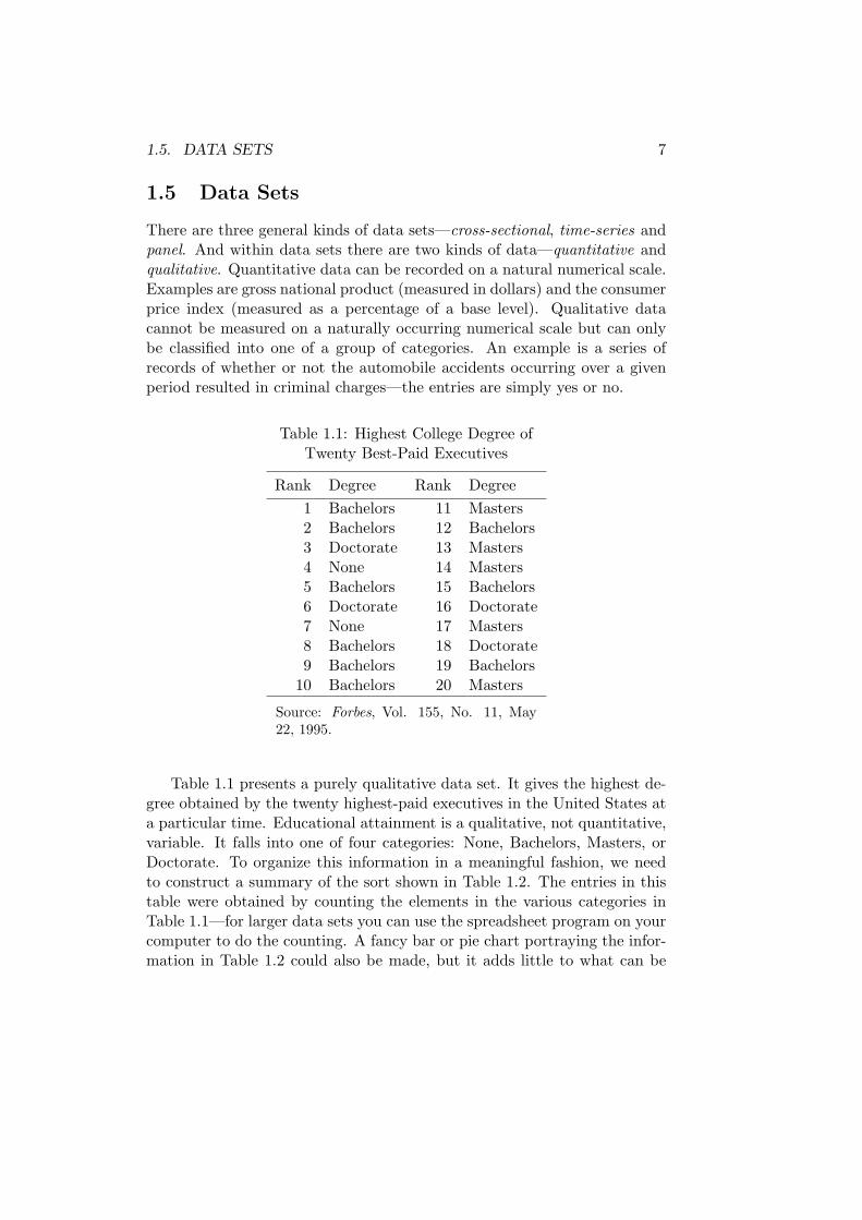
There are three general kinds of data sets—cross-sectional, time-series andpanel. And within data sets there are two kinds of data—quantitative andqualitative. Quantitative data can be recorded on a natural numerical scale.Examples are gross national product (measured in dollars) and the consumerprice index (measured as a percentage of a base level). Qualitative datacannot be measured on a naturally occurring numerical scale but can onlybe classified into one of a group of categories. An example is a series ofrecords of whether or not the automobile accidents occurring over a givenperiod resulted in criminal charges—the entries are simply yes or no.
Table 1.1: Highest College Degree ofTwenty Best-Paid Executives
Rank Degree Rank Degree
1 Bachelors 11 Masters2 Bachelors 12 Bachelors3 Doctorate 13 Masters4 None 14 Masters5 Bachelors 15 Bachelors6 Doctorate 16 Doctorate7 None 17 Masters8 Bachelors 18 Doctorate9 Bachelors 19 Bachelors
10 Bachelors 20 Masters
Source: Forbes, Vol. 155, No. 11, May22, 1995.
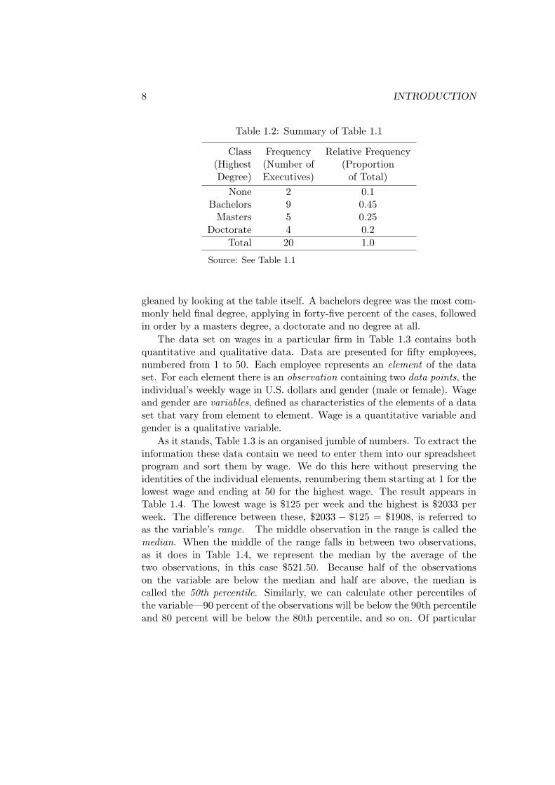
Table 1.1 presents a purely qualitative data set. It gives the highest de-gree obtained by the twenty highest-paid executives in the United States ata particular time. Educational attainment is a qualitative, not quantitative,variable. It falls into one of four categories: None, Bachelors, Masters, orDoctorate. To organize this information in a meaningful fashion, we needto construct a summary of the sort shown in Table 1.2. The entries in thistable were obtained by counting the elements in the various categories inTable 1.1—for larger data sets you can use the spreadsheet program on yourcomputer to do the counting. A fancy bar or pie chart portraying the infor-mation in Table 1.2 could also be made, but it adds little to what can be
8 INTRODUCTION
Table 1.2: Summary of Table 1.1
Class Frequency Relative Frequency(Highest (Number of (ProportionDegree) Executives) of Total)
None 2 0.1Bachelors 9 0.45Masters 5 0.25
Doctorate 4 0.2
Total 20 1.0
Source: See Table 1.1
gleaned by looking at the table itself. A bachelors degree was the most com-monly held final degree, applying in forty-five percent of the cases, followedin order by a masters degree, a doctorate and no degree at all.
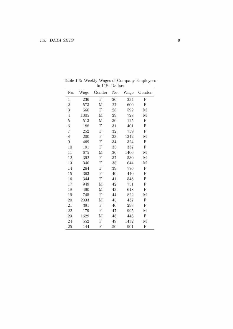
The data set on wages in a particular firm in Table 1.3 contains bothquantitative and qualitative data. Data are presented for fifty employees,numbered from 1 to 50. Each employee represents an element of the dataset. For each element there is an observation containing two data points, theindividual’s weekly wage in U.S. dollars and gender (male or female). Wageand gender are variables, defined as characteristics of the elements of a dataset that vary from element to element. Wage is a quantitative variable andgender is a qualitative variable.
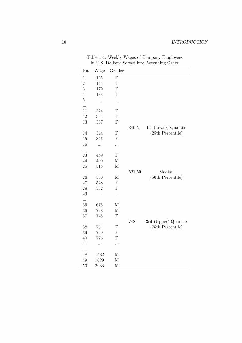
As it stands, Table 1.3 is an organised jumble of numbers. To extract theinformation these data contain we need to enter them into our spreadsheetprogram and sort them by wage. We do this here without preserving theidentities of the individual elements, renumbering them starting at 1 for thelowest wage and ending at 50 for the highest wage. The result appears inTable 1.4. The lowest wage is $125 per week and the highest is $2033 perweek. The difference between these, $2033 − $125 = $1908, is referred toas the variable’s range. The middle observation in the range is called themedian. When the middle of the range falls in between two observations,as it does in Table 1.4, we represent the median by the average of thetwo observations, in this case $521.50. Because half of the observationson the variable are below the median and half are above, the median iscalled the 50th percentile. Similarly, we can calculate other percentiles ofthe variable—90 percent of the observations will be below the 90th percentileand 80 percent will be below the 80th percentile, and so on. Of particular
1.5. DATA SETS 9
Table 1.3: Weekly Wages of Company Employeesin U.S. Dollars
No. Wage Gender No. Wage Gender
1 236 F 26 334 F2 573 M 27 600 F3 660 F 28 592 M4 1005 M 29 728 M5 513 M 30 125 F6 188 F 31 401 F7 252 F 32 759 F8 200 F 33 1342 M9 469 F 34 324 F10 191 F 35 337 F11 675 M 36 1406 M12 392 F 37 530 M13 346 F 38 644 M14 264 F 39 776 F15 363 F 40 440 F16 344 F 41 548 F17 949 M 42 751 F18 490 M 43 618 F19 745 F 44 822 M20 2033 M 45 437 F21 391 F 46 293 F22 179 F 47 995 M23 1629 M 48 446 F24 552 F 49 1432 M25 144 F 50 901 F
10 INTRODUCTION
Table 1.4: Weekly Wages of Company Employeesin U.S. Dollars: Sorted into Ascending Order
No. Wage Gender
1 125 F2 144 F3 179 F4 188 F5 ... ......11 324 F12 334 F13 337 F
340.5 1st (Lower) Quartile14 344 F (25th Percentile)15 346 F16 ... ......23 469 F24 490 M25 513 M
521.50 Median26 530 M (50th Percentile)27 548 F28 552 F29 ... ......35 675 M36 728 M37 745 F
748 3rd (Upper) Quartile38 751 F (75th Percentile)39 759 F40 776 F41 ... ......48 1432 M49 1629 M50 2033 M
1.5. DATA SETS 11
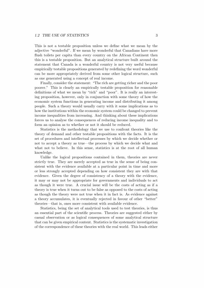
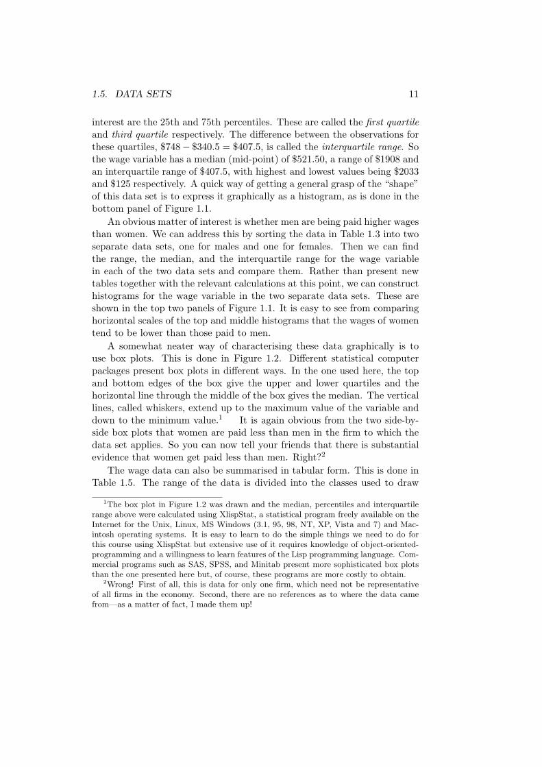
interest are the 25th and 75th percentiles. These are called the first quartileand third quartile respectively. The difference between the observations forthese quartiles, $748− $340.5 = $407.5, is called the interquartile range. Sothe wage variable has a median (mid-point) of $521.50, a range of $1908 andan interquartile range of $407.5, with highest and lowest values being $2033and $125 respectively. A quick way of getting a general grasp of the “shape”of this data set is to express it graphically as a histogram, as is done in thebottom panel of Figure 1.1.
An obvious matter of interest is whether men are being paid higher wagesthan women. We can address this by sorting the data in Table 1.3 into twoseparate data sets, one for males and one for females. Then we can findthe range, the median, and the interquartile range for the wage variablein each of the two data sets and compare them. Rather than present newtables together with the relevant calculations at this point, we can constructhistograms for the wage variable in the two separate data sets. These areshown in the top two panels of Figure 1.1. It is easy to see from comparinghorizontal scales of the top and middle histograms that the wages of womentend to be lower than those paid to men.
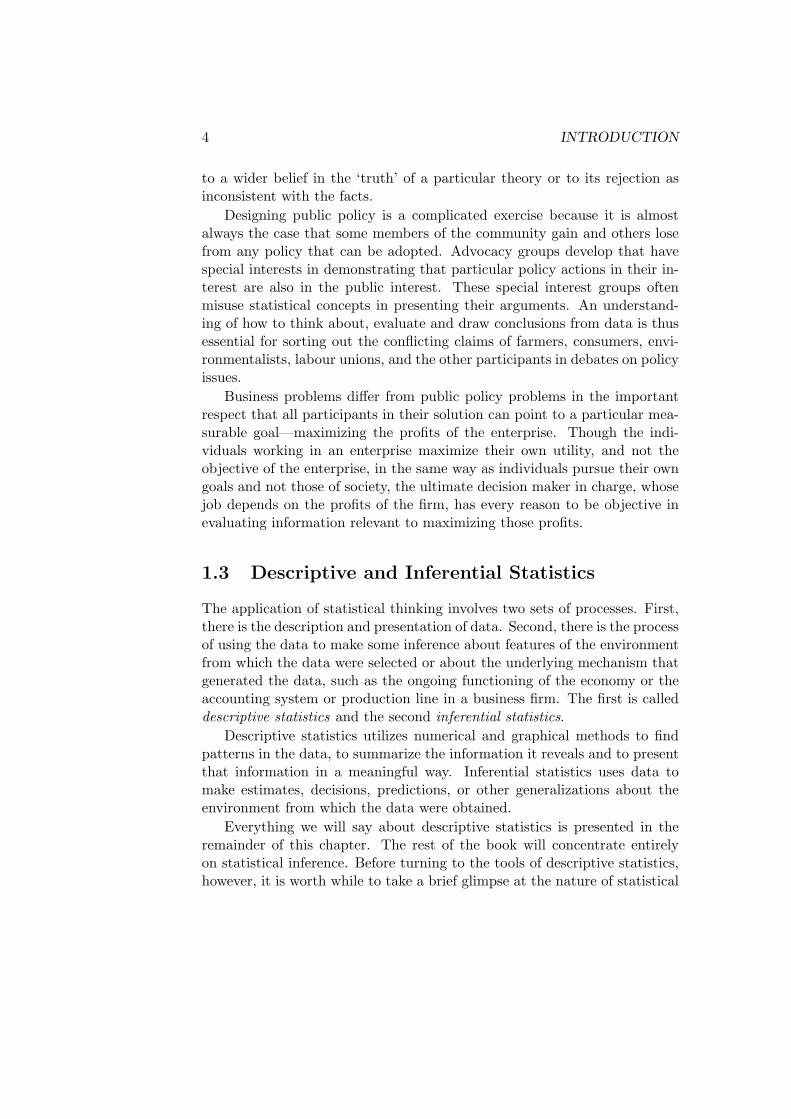
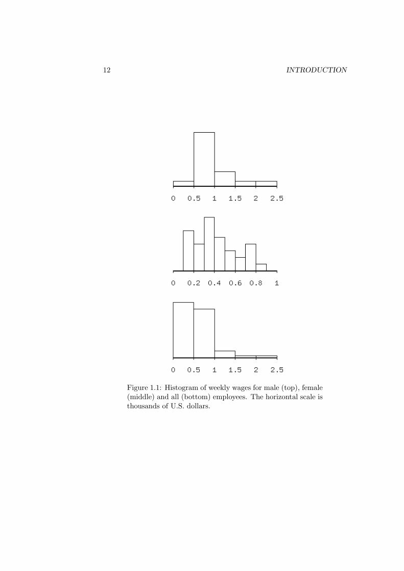
A somewhat neater way of characterising these data graphically is touse box plots. This is done in Figure 1.2. Different statistical computerpackages present box plots in different ways. In the one used here, the topand bottom edges of the box give the upper and lower quartiles and thehorizontal line through the middle of the box gives the median. The verticallines, called whiskers, extend up to the maximum value of the variable anddown to the minimum value.1 It is again obvious from the two side-by-side box plots that women are paid less than men in the firm to which thedata set applies. So you can now tell your friends that there is substantialevidence that women get paid less than men. Right?2
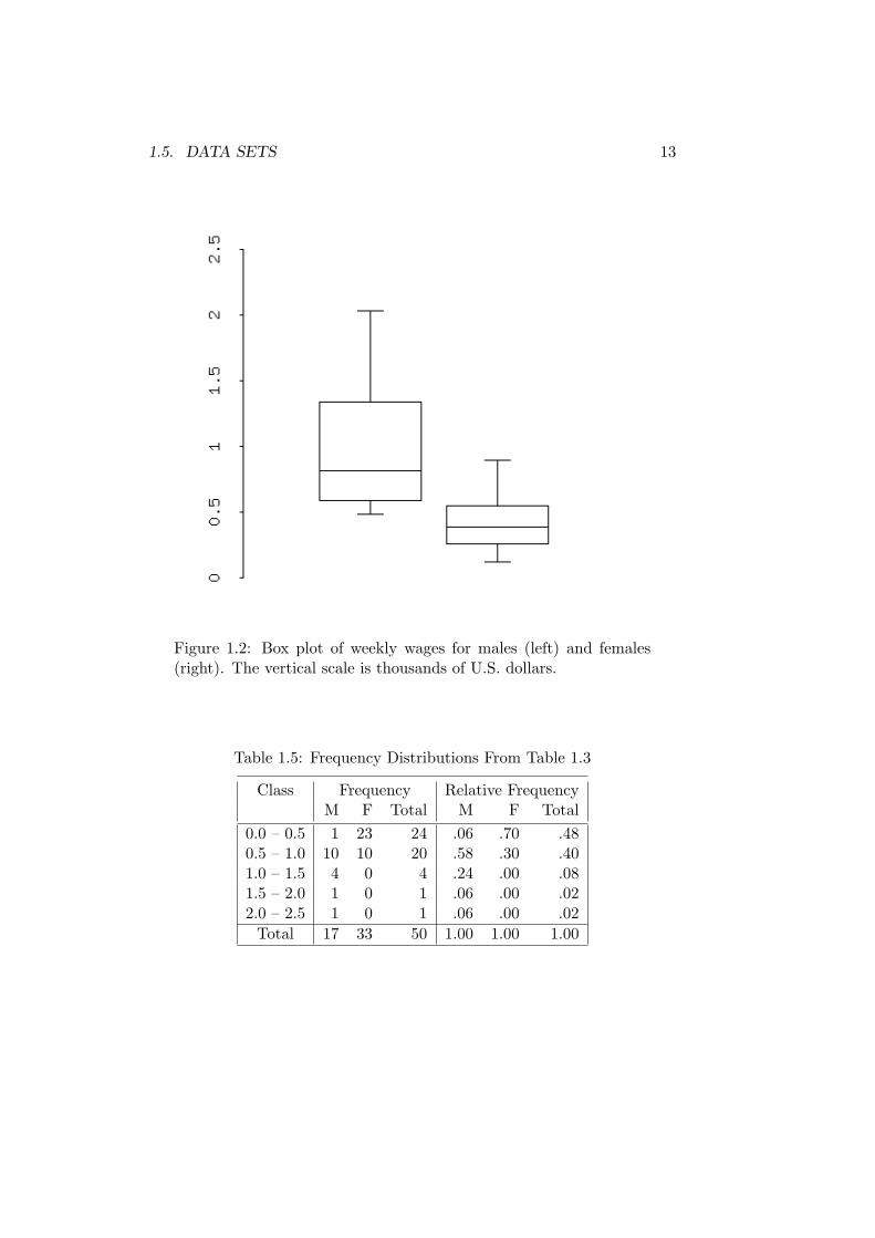
The wage data can also be summarised in tabular form. This is done inTable 1.5. The range of the data is divided into the classes used to draw
1The box plot in Figure 1.2 was drawn and the median, percentiles and interquartilerange above were calculated using XlispStat, a statistical program freely available on theInternet for the Unix, Linux, MS Windows (3.1, 95, 98, NT, XP, Vista and 7) and Mac-intosh operating systems. It is easy to learn to do the simple things we need to do forthis course using XlispStat but extensive use of it requires knowledge of object-oriented-programming and a willingness to learn features of the Lisp programming language. Com-mercial programs such as SAS, SPSS, and Minitab present more sophisticated box plotsthan the one presented here but, of course, these programs are more costly to obtain.
2Wrong! First of all, this is data for only one firm, which need not be representativeof all firms in the economy. Second, there are no references as to where the data camefrom—as a matter of fact, I made them up!
12 INTRODUCTION
Figure 1.1: Histogram of weekly wages for male (top), female(middle) and all (bottom) employees. The horizontal scale isthousands of U.S. dollars.
1.5. DATA SETS 13
Figure 1.2: Box plot of weekly wages for males (left) and females(right). The vertical scale is thousands of U.S. dollars.
Table 1.5: Frequency Distributions From Table 1.3
Class Frequency Relative FrequencyM F Total M F Total
0.0 – 0.5 1 23 24 .06 .70 .480.5 – 1.0 10 10 20 .58 .30 .401.0 – 1.5 4 0 4 .24 .00 .081.5 – 2.0 1 0 1 .06 .00 .022.0 – 2.5 1 0 1 .06 .00 .02
Total 17 33 50 1.00 1.00 1.00
14 INTRODUCTION
the histogram for the full data set. Then the observations for the wagevariable in Table 1.3 that fall in each of the classes are counted and thenumbers entered into the appropriate cells in columns 2, 3 and 4 of thetable. The observations are thus ‘distributed’ among the classes with thenumbers in the cells indicating the ‘frequency’ with which observations fallin the respective classes—hence, such tables present frequency distributions.The totals along the bottom tell us that there were 17 men and 33 women,with a total of 50 elements in the data set. The relative frequencies in whichobservations fall in the classes are shown in columns 5, 6 and 7. Column 5gives the proportions of men’s wages, column 6 the proportions of women’swages and column 7 the proportions of all wages falling in the classes. Theproportions in each column must add up to one.
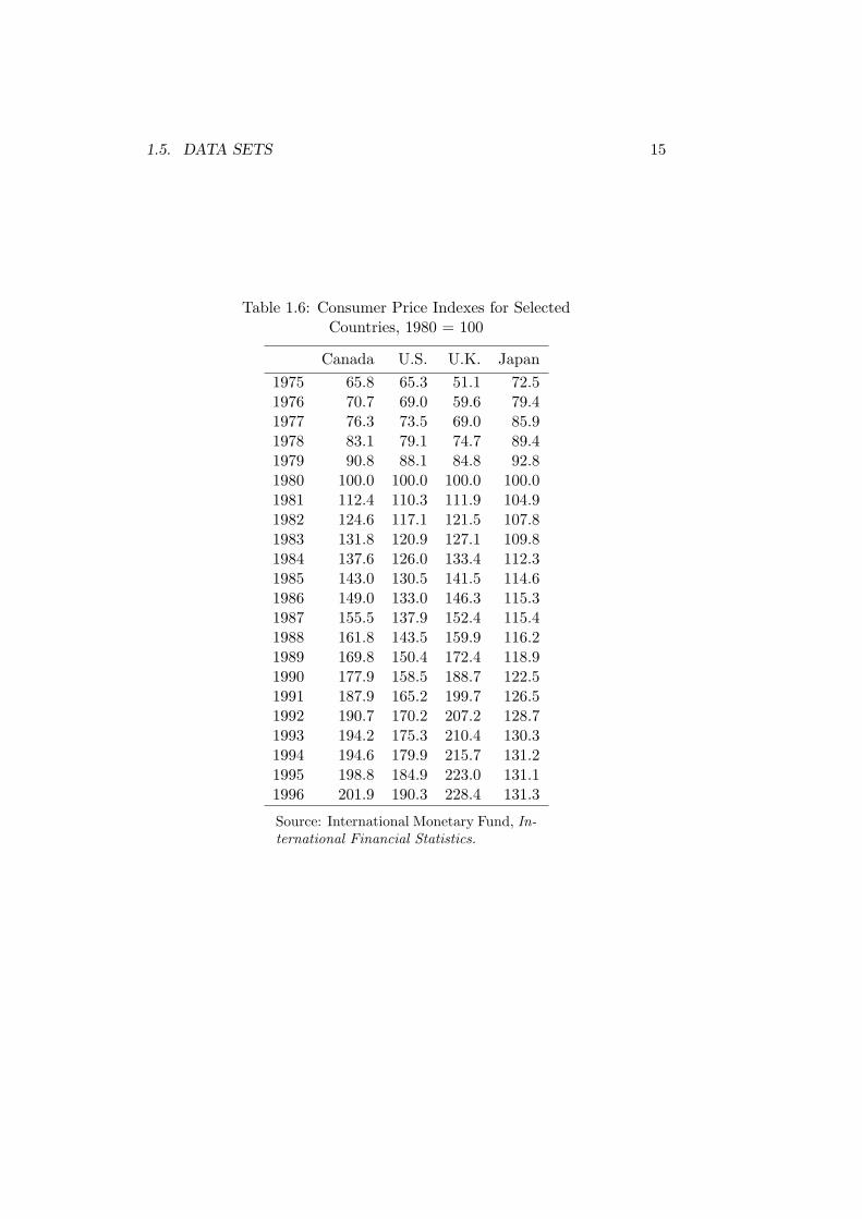
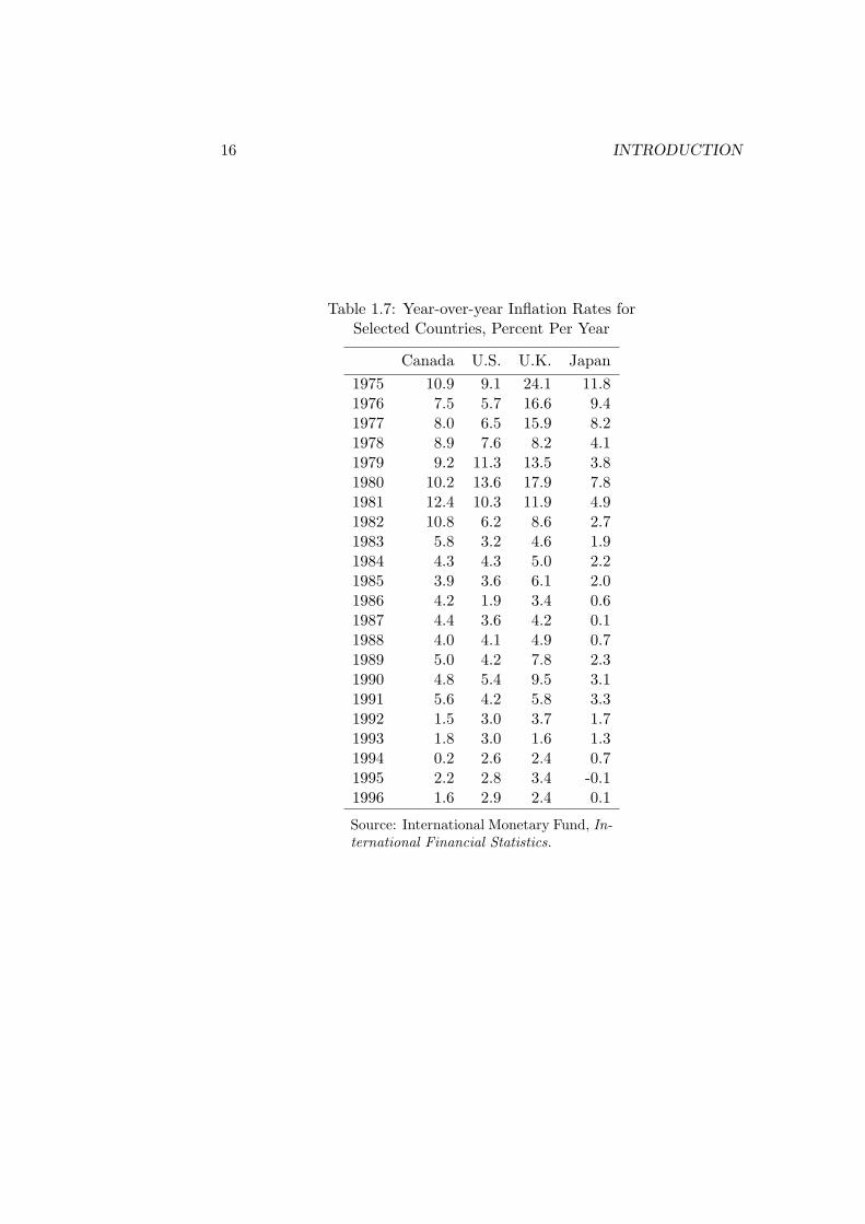
All of the data sets considered thus far are cross-sectional. Tables 1.6 and1.7 present time-series data sets. The first table gives the consumer priceindexes for four countries, Canada, the United States, the United Kingdomand Japan, for the years 1975 to 1996.3 The second table presents the year-over-year inflation rates for the same period for these same countries. Theinflation rates are calculated as
π = [100(Pt − Pt−1)/Pt−1]
where π denotes the inflation rate and P denotes the consumer price index.It should now be obvious that in time-series data the elements are units oftime. This distinguishes time-series from cross-sectional data sets, where allobservations occur in the same time period.
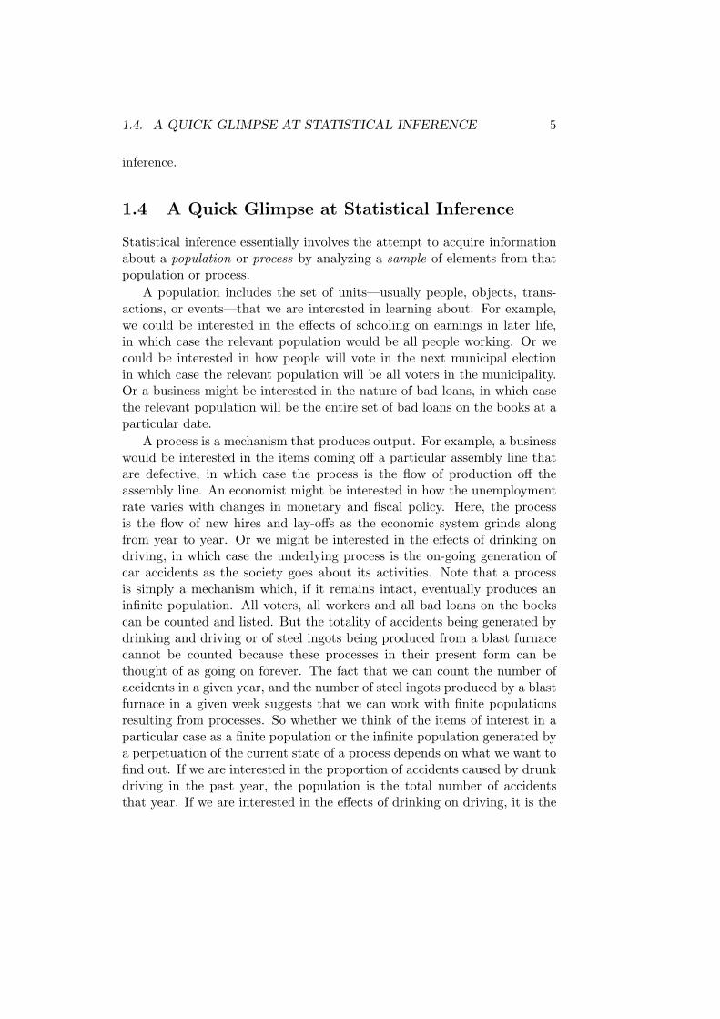
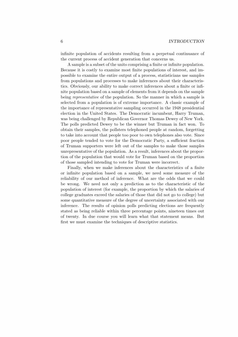
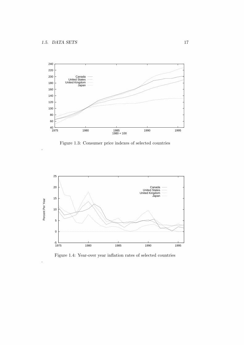
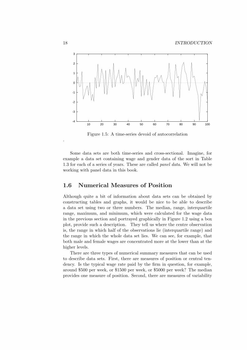
A frequent feature of time-series data not present in cross-sectional datais serial correlation or autocorrelation. The data in Tables 1.6 and 1.7are plotted in Figures 1.3 and 1.4 respectively. You will notice from theseplots that one can make a pretty good guess as to what the price level orinflation rate will be in a given year on the basis of the observed price leveland inflation rate in previous years. If prices or inflation are high this year,they will most likely also be high next year. Successive observations in eachseries are serially correlated or autocorrelated (i.e., correlated through time)and hence not statistically independent of each other. Figure 1.5 shows atime-series that has no autocorrelation—the successive observations weregenerated completely independently of all preceding observations using acomputer. You will learn more about correlation and statistical indepen-dence later in this chapter.
3Consumer price indexes are calculated by taking the value in each year of the bundleof goods consumed by a typical person as a percentage of the monetary value of that samebundle of goods in a base period. In Table 1.6 the base year is 1980.
1.5. DATA SETS 15
Table 1.6: Consumer Price Indexes for SelectedCountries, 1980 = 100
Canada U.S. U.K. Japan
1975 65.8 65.3 51.1 72.51976 70.7 69.0 59.6 79.41977 76.3 73.5 69.0 85.91978 83.1 79.1 74.7 89.41979 90.8 88.1 84.8 92.81980 100.0 100.0 100.0 100.01981 112.4 110.3 111.9 104.91982 124.6 117.1 121.5 107.81983 131.8 120.9 127.1 109.81984 137.6 126.0 133.4 112.31985 143.0 130.5 141.5 114.61986 149.0 133.0 146.3 115.31987 155.5 137.9 152.4 115.41988 161.8 143.5 159.9 116.21989 169.8 150.4 172.4 118.91990 177.9 158.5 188.7 122.51991 187.9 165.2 199.7 126.51992 190.7 170.2 207.2 128.71993 194.2 175.3 210.4 130.31994 194.6 179.9 215.7 131.21995 198.8 184.9 223.0 131.11996 201.9 190.3 228.4 131.3
Source: International Monetary Fund, In-ternational Financial Statistics.
16 INTRODUCTION
Table 1.7: Year-over-year Inflation Rates forSelected Countries, Percent Per Year
Canada U.S. U.K. Japan
1975 10.9 9.1 24.1 11.81976 7.5 5.7 16.6 9.41977 8.0 6.5 15.9 8.21978 8.9 7.6 8.2 4.11979 9.2 11.3 13.5 3.81980 10.2 13.6 17.9 7.81981 12.4 10.3 11.9 4.91982 10.8 6.2 8.6 2.71983 5.8 3.2 4.6 1.91984 4.3 4.3 5.0 2.21985 3.9 3.6 6.1 2.01986 4.2 1.9 3.4 0.61987 4.4 3.6 4.2 0.11988 4.0 4.1 4.9 0.71989 5.0 4.2 7.8 2.31990 4.8 5.4 9.5 3.11991 5.6 4.2 5.8 3.31992 1.5 3.0 3.7 1.71993 1.8 3.0 1.6 1.31994 0.2 2.6 2.4 0.71995 2.2 2.8 3.4 -0.11996 1.6 2.9 2.4 0.1
Source: International Monetary Fund, In-ternational Financial Statistics.
1.5. DATA SETS 17
40
60
80
100
120
140
160
180
200
220
240
1975 1980 1985 1990 19951980 = 100
CanadaUnited States
United KingdomJapan
Figure 1.3: Consumer price indexes of selected countries.
-5
0
5
10
15
20
25
1975 1980 1985 1990 1995
Per
cent
Per
Yea
r
CanadaUnited States
United KingdomJapan
Figure 1.4: Year-over year inflation rates of selected countries.
18 INTRODUCTION
-4
-3
-2
-1
0
1
2
3
10 20 30 40 50 60 70 80 90 100
Figure 1.5: A time-series devoid of autocorrelation.
Some data sets are both time-series and cross-sectional. Imagine, forexample a data set containing wage and gender data of the sort in Table1.3 for each of a series of years. These are called panel data. We will not beworking with panel data in this book.
1.6 Numerical Measures of Position
Although quite a bit of information about data sets can be obtained byconstructing tables and graphs, it would be nice to be able to describea data set using two or three numbers. The median, range, interquartilerange, maximum, and minimum, which were calculated for the wage datain the previous section and portrayed graphically in Figure 1.2 using a boxplot, provide such a description. They tell us where the centre observationis, the range in which half of the observations lie (interquartile range) andthe range in which the whole data set lies. We can see, for example, thatboth male and female wages are concentrated more at the lower than at thehigher levels.
There are three types of numerical summary measures that can be usedto describe data sets. First, there are measures of position or central ten-dency. Is the typical wage rate paid by the firm in question, for example,around $500 per week, or $1500 per week, or $5000 per week? The medianprovides one measure of position. Second, there are measures of variability
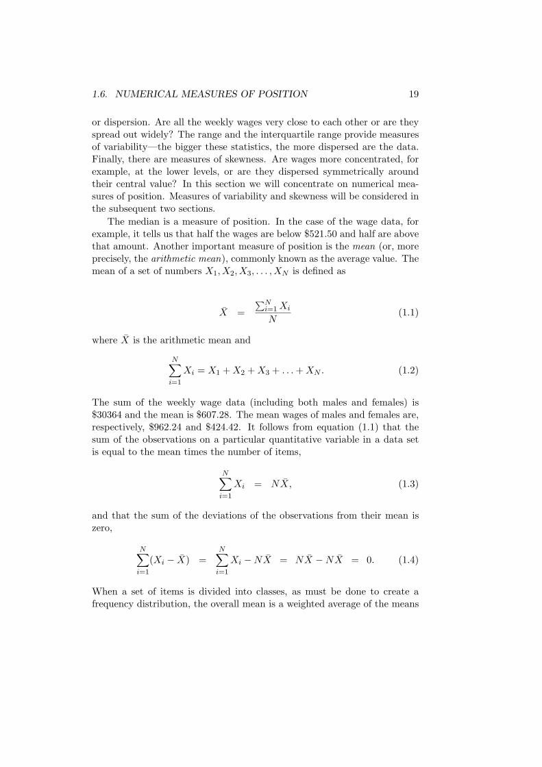
1.6. NUMERICAL MEASURES OF POSITION 19
or dispersion. Are all the weekly wages very close to each other or are theyspread out widely? The range and the interquartile range provide measuresof variability—the bigger these statistics, the more dispersed are the data.Finally, there are measures of skewness. Are wages more concentrated, forexample, at the lower levels, or are they dispersed symmetrically aroundtheir central value? In this section we will concentrate on numerical mea-sures of position. Measures of variability and skewness will be considered inthe subsequent two sections.
The median is a measure of position. In the case of the wage data, forexample, it tells us that half the wages are below $521.50 and half are abovethat amount. Another important measure of position is the mean (or, moreprecisely, the arithmetic mean), commonly known as the average value. Themean of a set of numbers X1, X2, X3, . . . , XN is defined as
X =
∑Ni=1Xi
N(1.1)
where X is the arithmetic mean and
N∑i=1
Xi = X1 +X2 +X3 + . . .+XN . (1.2)
The sum of the weekly wage data (including both males and females) is$30364 and the mean is $607.28. The mean wages of males and females are,respectively, $962.24 and $424.42. It follows from equation (1.1) that thesum of the observations on a particular quantitative variable in a data setis equal to the mean times the number of items,
N∑i=1
Xi = NX, (1.3)
and that the sum of the deviations of the observations from their mean iszero,
N∑i=1
(Xi − X) =N∑i=1
Xi −NX = NX −NX = 0. (1.4)
When a set of items is divided into classes, as must be done to create afrequency distribution, the overall mean is a weighted average of the means

20 INTRODUCTION
of the observations in the classes, with the weights being the number (orfrequency) of items in the respective classes. When there are k classes,
X =f1X1 + f2X2 + f3X3 + . . .+ fkXk
N=
∑ki=1 fiXi
N(1.5)
where Xi is the mean of the observations in the ith class and fi is thenumber (frequency) of observations in the ith class. If all that is known isthe frequency in each class with no measure of the mean of the observationsin the classes available, we can obtain a useful approximation to the meanof the data set using the mid-points of the classes in the above formula inplace of the class means.
An alternative mean value is the geometric mean which is defined asthe anti-log of the arithmetic mean of the logarithms of the values. Thegeometric mean can thus be obtained by taking the anti-log of
logX1 + logX2 + logX3 + . . .+ logXN
N
or the nth root of X1X2X3 . . . XN .4 Placing a bar on top of a variableto denote its mean, as in X, is done only to represent means of samples.The mean of a population is represented by the Greek symbol µ. Whenthe population is finite, µ can be obtained by making the calculation inequation 1.1 using all elements in the population. The mean of an infinitepopulation generated by a process has to be derived from the mathematicalrepresentation of that process. In most practical cases this mathematicaldata generating process is unknown. The ease of obtaining the means offinite as opposed to infinite populations is more apparent than real. Thecost of calculating the mean for large finite populations is usually prohibitivebecause a census of the entire population is required.
The mean is strongly influenced by extreme values in the data set. Forexample, suppose that the members of a small group of eight people havethe following annual incomes in dollars: 24000, 23800, 22950, 26000, 275000,25500, 24500, 23650. We want to present a single number that characterises
4Note from the definition of logarithms that taking the logarithm of the nth root of(X1X2X3 . . . XN ), which equals
(X1X2X3 . . . XN )1N ,
yieldslogX1 + logX2 + logX3 + . . .+ logXN
N.
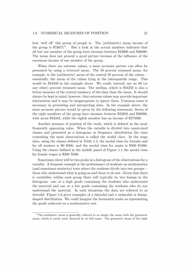
1.6. NUMERICAL MEASURES OF POSITION 21
how ‘well off’ this group of people is. The (arithmetic) mean income ofthe group is $55675.5 But a look at the actual numbers indicates thatall but one member of the group have incomes between $23000 and $26000.The mean does not present a good picture because of the influence of theenormous income of one member of the group.
When there are extreme values, a more accurate picture can often bepresented by using a trimmed mean. The 50 percent trimmed mean, forexample, is the (arithmetic) mean of the central 50 percent of the values—essentially, the mean of the values lying in the interquartile range. Thiswould be $24450 in the example above. We could, instead, use an 80 (orany other) percent trimmed mean. The median, which is $24250 is also abetter measure of the central tendency of the data than the mean. It shouldalways be kept in mind, however, that extreme values may provide importantinformation and it may be inappropriate to ignore them. Common sense isnecessary in presenting and interpreting data. In the example above, themost accurate picture would be given by the following statement: Seven ofthe eight members of the group have incomes between $22950 and $26000,with mean $24342, while the eighth member has an income of $275000.
Another measure of position of the mode, which is defined as the mostfrequently appearing value. When the variable is divided into equal-sizedclasses and presented as a histogram or frequency distribution the classcontaining the most observations is called the modal class. In the wagedata, using the classes defined in Table 1.5, the modal class for females andfor all workers is $0–$500, and the modal class for males is $500–$1000.Using the classes defined in the middle panel of Figure 1.1 the modal classfor female wages is $300–$400.
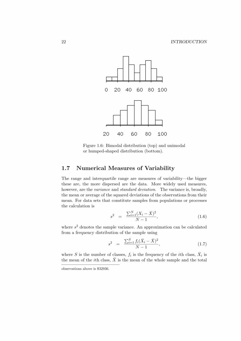
Sometimes there will be two peaks in a histogram of the observations for avariable. A frequent example is the performance of students on mathematics(and sometimes statistics) tests where the students divide into two groups—those who understand what is going on and those to do not. Given that thereis variability within each group there will typically be two humps in thehistogram—one at a high grade containing the students who understandthe material and one at a low grade containing the students who do notunderstand the material. In such situations the data are referred to asbimodal. Figure 1.6 gives examples of a bimodal and a unimodal or hump-shaped distribution. We could imagine the horizontal scales as representingthe grade achieved on a mathematics test.
5The arithmetic mean is generally referred to as simply the mean with the geometricmean, which is rarely used, denoted by its full name. The geometric mean of the eight
22 INTRODUCTION
Figure 1.6: Bimodal distribution (top) and unimodalor humped-shaped distribution (bottom).
1.7 Numerical Measures of Variability
The range and interquartile range are measures of variability—the biggerthese are, the more dispersed are the data. More widely used measures,however, are the variance and standard deviation. The variance is, broadly,the mean or average of the squared deviations of the observations from theirmean. For data sets that constitute samples from populations or processesthe calculation is
s2 =
∑Ni=1(Xi − X)2
N − 1, (1.6)
where s2 denotes the sample variance. An approximation can be calculatedfrom a frequency distribution of the sample using
s2 =
∑Si=1 fi(Xi − X)2
N − 1, (1.7)
where S is the number of classes, fi is the frequency of the ith class, Xi isthe mean of the ith class, X is the mean of the whole sample and the total
observations above is $32936.
1.7. NUMERICAL MEASURES OF VARIABILITY 23
number of elements in the sample equals
N =S∑
i=1
fi.
The population variance is denoted by σ2. For a finite population it can becalculated using (1.6) after replacing N −1 in the denominator by N . N −1is used in the denominator in calculating the sample variance because thevariance is the mean of the sum of squared independent deviations from thesample mean and only N − 1 of the N deviations from the sample meancan be independently selected—once we know N − 1 of the deviations, theremaining one can be calculated from those already known based on theway the sample mean was calculated. Each sample from a given populationwill have a different sample mean, depending upon the population elementsthat appear in it. The population mean, on the other hand, is a fixednumber which does not change from sample to sample. The deviations of thepopulation elements from the population mean are therefore all independentof each other. In the case of a process, the exact population variance can onlybe obtained from knowledge of the mathematical data-generation process.
In the weekly wage data above, the variance of wages is 207161.5 formales, 42898.7 for females and 161893.7 for the entire sample. Notice thatthe units in which these variances are measured is dollars-squared—we aretaking the sum of the squared dollar-differences of each person’s wage fromthe mean. To obtain a measure of variability measured in dollars rather thandollars-squared we can take the square root of the variance—s in equation(1.6). This is called the standard deviation. The standard deviation of wagesin the above sample is $455.15 for males, $207.12 for females, and $402.36for the entire sample.
Another frequently used measure of variability is the coefficient of vari-ation, defined as the standard deviation taken as a percentage of the mean,
C =100s
X, (1.8)
where C denotes the coefficient of variation. For the weekly wage dataabove, the coefficient of variation is 47.30 for males, 48.8 for females and66.28 for the entire sample.
24 INTRODUCTION
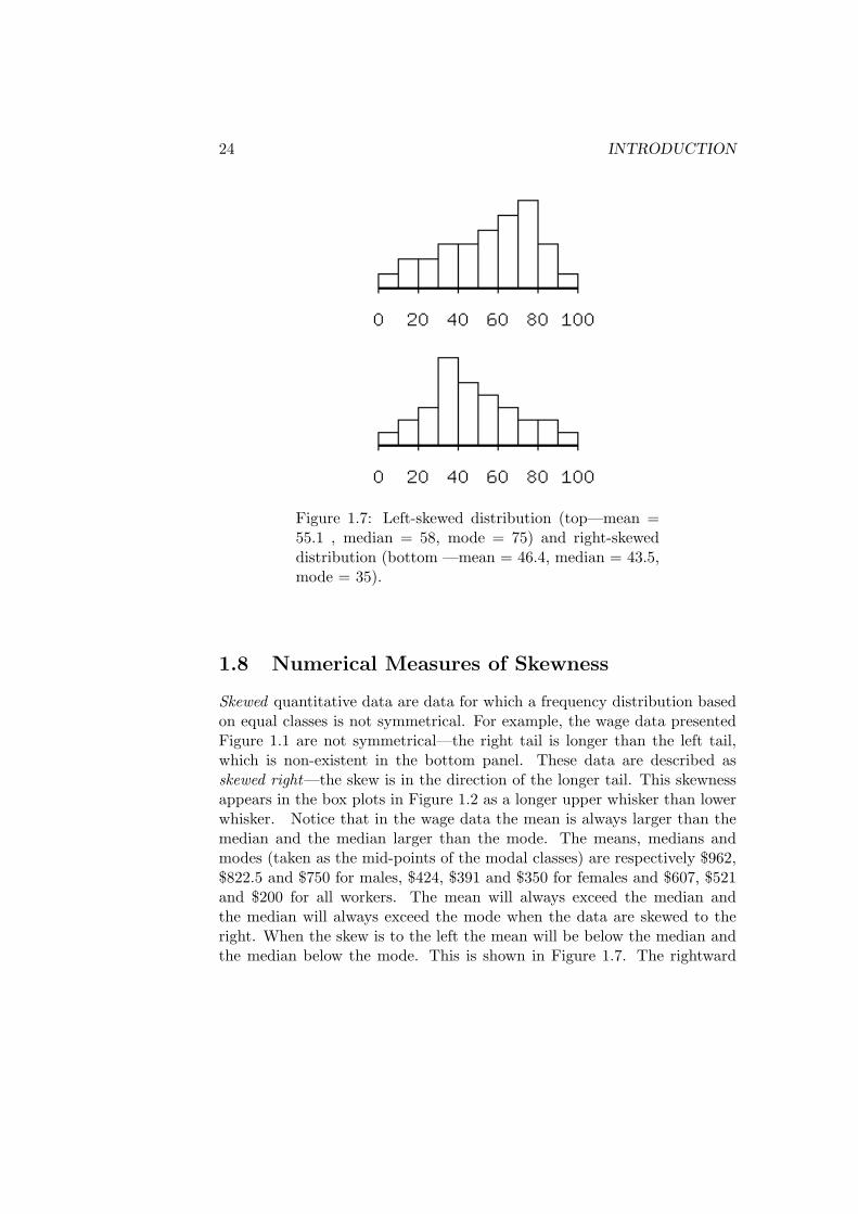
Figure 1.7: Left-skewed distribution (top—mean =55.1 , median = 58, mode = 75) and right-skeweddistribution (bottom —mean = 46.4, median = 43.5,mode = 35).
1.8 Numerical Measures of Skewness
Skewed quantitative data are data for which a frequency distribution basedon equal classes is not symmetrical. For example, the wage data presentedFigure 1.1 are not symmetrical—the right tail is longer than the left tail,which is non-existent in the bottom panel. These data are described asskewed right—the skew is in the direction of the longer tail. This skewnessappears in the box plots in Figure 1.2 as a longer upper whisker than lowerwhisker. Notice that in the wage data the mean is always larger than themedian and the median larger than the mode. The means, medians andmodes (taken as the mid-points of the modal classes) are respectively $962,$822.5 and $750 for males, $424, $391 and $350 for females and $607, $521and $200 for all workers. The mean will always exceed the median andthe median will always exceed the mode when the data are skewed to theright. When the skew is to the left the mean will be below the median andthe median below the mode. This is shown in Figure 1.7. The rightward
1.8 STANDARDISED VALUES 25
(leftward) skew is due to the influence of the rather few unusually high(low) values—the extreme values drag the mean in their direction. Themedian tends to be above the mode when the data are skewed right becauselow values are more frequent than high values and below the mode whenthe data are skewed to the left because in that case high values are morefrequent than low values. When the data are symmetrically distributed, themean, median and mode are equal.
Skewness can be measured by the average cubed deviation of the valuesfrom the sample mean,
m3 =
∑Ni=1(Xi − X)3
N − 1. (1.9)
If the large deviations are predominately positive m3 will be positive and ifthe large deviations are predominately negative m3 will be negative. Thishappens because (Xi − X)3 has the same sign as (Xi − X). Since largedeviations are associated with the long tail of the frequency distribution, m3
will be positive or negative according to whether the direction of skewness ispositive (right) or negative (left). In the wage data m3 is positive for males,females and all workers as we would expect from looking at figures 1.1 and1.2.
1.9 Numerical Measures of Relative Position:Standardised Values
In addition to measures of the central tendency of a set of values and theirdispersion around these central measures we are often interested in whethera particular observation is high or low relative to others in the set. Onemeasure of this is the percentile in which the observation falls—if an ob-servation is at the 90th percentile, only 10% of the values lie above it and90% percent of the values lie below it. Another measure of relative positionis the standardised value. The standardised value of an observation is itsdistance from the mean divided by the standard deviation of the sample orpopulation in which the observation is located. The standardised values ofthe set of observations X1, X2, X3 . . . XN are given by
Zi =Xi − µ
σ(1.10)
26 INTRODUCTION
for members of a population whose mean µ and standard deviation σ areknown and
Zi =Xi − X
s(1.11)
for members of a sample with mean X and sample standard deviation s. Thestandardised value or z-value of an observation is the number of standarddeviations it is away from the mean.
It turns out that for a distribution that is hump-shaped—that is, notbimodal—roughly 68% of the observations will lie within plus or minus onestandard deviation from the mean, about 95% of the values will lie withinplus or minus two standard deviations from the mean, and roughly 99.7%of the observations will lie within plus or minus three standard deviationsfrom the mean. Thus, if you obtain a grade of 52% percent on a statisticstest for which the class average was 40% percent and the standard deviation10% percent, and the distribution is hump-shaped rather than bimodal, youare probably in the top 16 percent of the class. This calculation is madeby noting that about 68 percent of the class will score within one standarddeviation from 40—that is, between 30 and 50—and 32 percent will scoreoutside that range. If the two tails of the distribution are equally populatedthen you must be in the top 16% percent of the class. Relatively speaking,52% was a pretty good grade.
The above percentages hold almost exactly for normal distributions,which you will learn about in due course, and only approximately for hump-shaped distributions that do not satisfy the criteria for normality. Theydo not hold for distributions that are bimodal. It turns out that there isa rule developed by the Russian mathematician P. L. Chebyshev, calledChebyshev’s Inequality, which states that a fraction no bigger than (1/k)2
(or 100 × (1/k)2 percent) of any set of observations, no matter what theshape of their distribution, will lie beyond plus or minus k standard devia-tions from the mean of those observations. So if the standard deviation is 2at least 75% of the distribution must lie within plus or minus two standarddeviations from the mean and no more than 25% percent of the distributioncan lie outside that range in one or other of the tails. You should note espe-cially that the rule does not imply here that no more than 12.5% percent ofa distribution will lie two standard deviations above the mean because thedistribution need not be symmetrical.
1.9 COVARIANCE AND CORRELATION 27
1.10 Bivariate Data: Covariance and Correlation
A data set that contains only one variable of interest, as would be the casewith the wage data above if the gender of each wage earner was not recorded,is called a univariate data set. Data sets that contain two variables, suchas wage and gender in the wage data above, are said to be bivariate. Andthe consumer price index and inflation rate data presented in Table 1.6and Table 1.7 above are multivariate, with each data set containing fourvariables—consumer price indexes or inflation rates for four countries.
In the case of bivariate or multivariate data sets we are often interestedin whether elements that have high values of one of the variables also havehigh values of other variables. For example, as students of economics wemight be interested in whether people with more years of schooling earnhigher incomes. From Canadian Government census data we might obtainfor the population of all Canadian households two quantitative variables,household income (measured in $) and number of years of education of thehead of each household.6 Let Xi be the value of annual household incomefor household i and Yi be the number of years of schooling of the head ofthe ith household. Now consider a random sample of N households whichyields the paired observations (Xi, Yi) for i = 1, 2, 3, . . . , N .
You already know how to create summary statistical measures for singlevariables. The sample mean value for household incomes, for example, canbe obtained by summing up all the Xi and dividing the resulting sum byN . And the sample mean value for years of education per household cansimilarly be obtained by summing all the Yi and dividing by N . We can alsocalculate the sample variances of X and Y by applying equation (1.6).
Notice that the fact that the sample consists of paired observations(Xi, Yi) is irrelevant when we calculate summary measures for the individualvariables X and/or Y . Nevertheless, we may also be interested in whetherthe variables X and Y are related to one another in a systematic way. Sinceeducation is a form of investment that yields its return in the form of higherlifetime earnings, we might expect, for example, that household income willtend to be higher the greater the number of years of education completedby the head of household. That is, we might expect high values of X tobe paired with high values of Y—when Xi is high, the Yi associated with itshould also be high, and vice versa.
Another example is the consumer price indexes and inflation rates for
6This example and most of the prose in this section draws on the expositional effortsof Prof. Greg Jump, my colleague at the University of Toronto.
28 INTRODUCTION
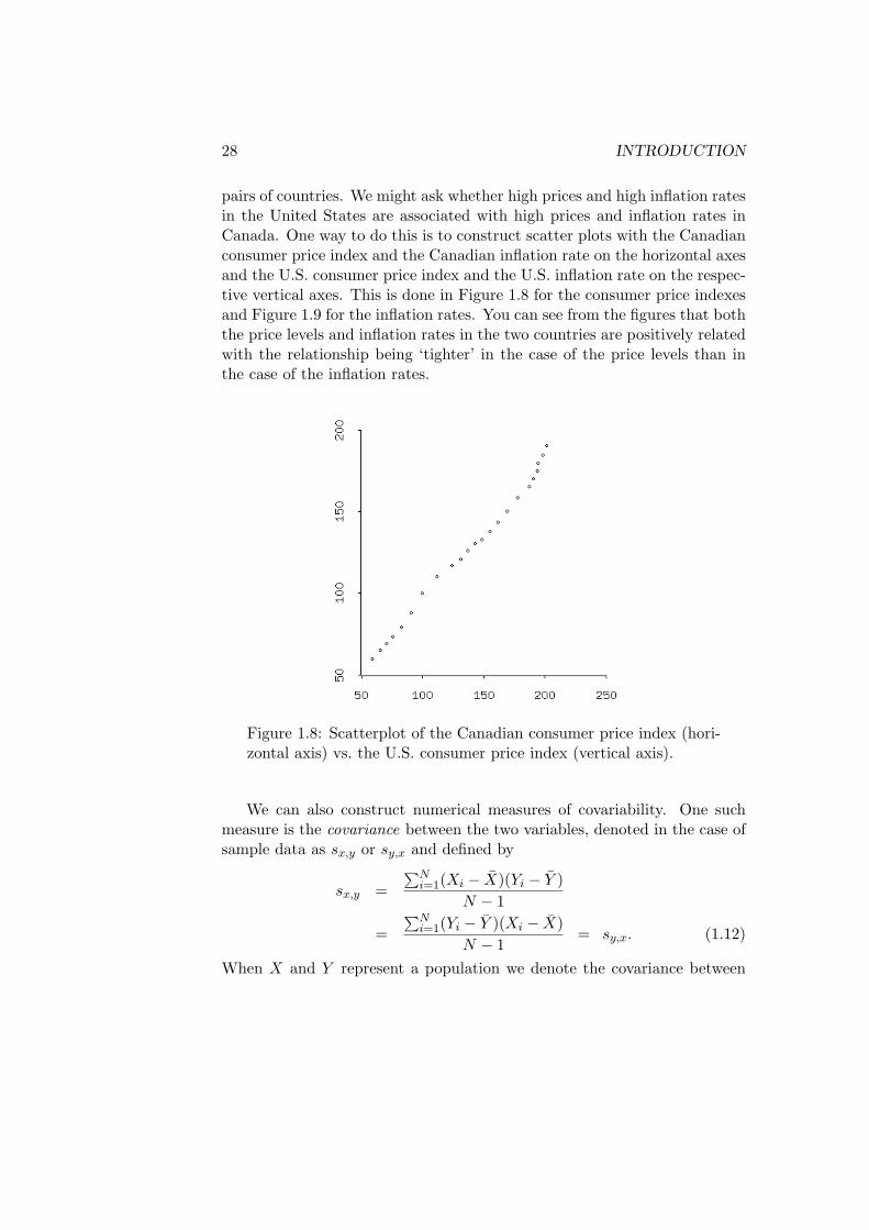
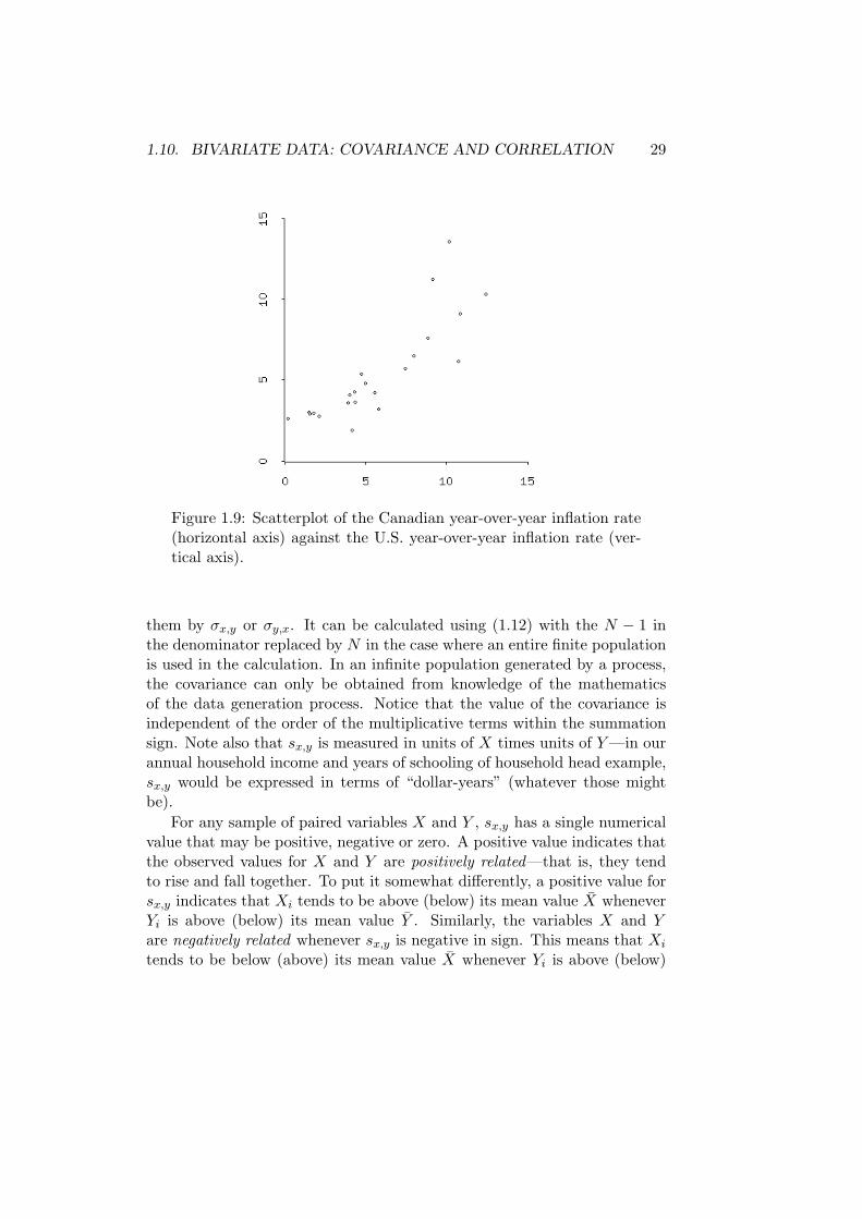
pairs of countries. We might ask whether high prices and high inflation ratesin the United States are associated with high prices and inflation rates inCanada. One way to do this is to construct scatter plots with the Canadianconsumer price index and the Canadian inflation rate on the horizontal axesand the U.S. consumer price index and the U.S. inflation rate on the respec-tive vertical axes. This is done in Figure 1.8 for the consumer price indexesand Figure 1.9 for the inflation rates. You can see from the figures that boththe price levels and inflation rates in the two countries are positively relatedwith the relationship being ‘tighter’ in the case of the price levels than inthe case of the inflation rates.
Figure 1.8: Scatterplot of the Canadian consumer price index (hori-zontal axis) vs. the U.S. consumer price index (vertical axis).
We can also construct numerical measures of covariability. One suchmeasure is the covariance between the two variables, denoted in the case ofsample data as sx,y or sy,x and defined by
sx,y =
∑Ni=1(Xi − X)(Yi − Y )
N − 1
=
∑Ni=1(Yi − Y )(Xi − X)
N − 1= sy,x. (1.12)
When X and Y represent a population we denote the covariance between
1.10. BIVARIATE DATA: COVARIANCE AND CORRELATION 29
Figure 1.9: Scatterplot of the Canadian year-over-year inflation rate(horizontal axis) against the U.S. year-over-year inflation rate (ver-tical axis).
them by σx,y or σy,x. It can be calculated using (1.12) with the N − 1 inthe denominator replaced by N in the case where an entire finite populationis used in the calculation. In an infinite population generated by a process,the covariance can only be obtained from knowledge of the mathematicsof the data generation process. Notice that the value of the covariance isindependent of the order of the multiplicative terms within the summationsign. Note also that sx,y is measured in units of X times units of Y—in ourannual household income and years of schooling of household head example,sx,y would be expressed in terms of “dollar-years” (whatever those mightbe).
For any sample of paired variables X and Y , sx,y has a single numericalvalue that may be positive, negative or zero. A positive value indicates thatthe observed values for X and Y are positively related—that is, they tendto rise and fall together. To put it somewhat differently, a positive value forsx,y indicates that Xi tends to be above (below) its mean value X wheneverYi is above (below) its mean value Y . Similarly, the variables X and Yare negatively related whenever sx,y is negative in sign. This means that Xi
tends to be below (above) its mean value X whenever Yi is above (below)
30 INTRODUCTION
its mean value Y . When there is no relationship between the variables Xand Y , sx,y is zero.
In our household income and education example we would expect thata random sample would yield a positive value for sx,y and this is indeedwhat is found in actual samples drawn from the population of all Canadianhouseholds.
Note that equation (1.12) could be used to compute sx,x—the covarianceof the variable X with itself. It is easy to see from equations (1.12) and (1.6)that this will yield the sample variance of X which we can denote by s2x. Itmight be thus said that the concept of variance is just a special case of themore general concept of covariance.
The concept of covariance is important in the study of financial eco-nomics because it is critical to an understanding of ‘risk’ in securities andother asset markets. Unfortunately, it is a concept that yields numbers thatare not very ‘intuitive’. For example, suppose we were to find that a sam-ple of N Canadian households yields a covariance of +1, 000 dollar-yearsbetween annual household income and years of education of head of house-hold. The covariance is positive in sign, so we know that this implies thathouseholds with highly educated heads tend to have high annual incomes.But is there any intuitive interpretation of the magnitude 1000 dollar-years?The answer is no, at least not without further information regarding the in-dividual sample variances of household income and age of head.
A more intuitive concept, closely related to covariance, is the correlationbetween two variables. The coefficient of correlation between two variablesX and Y , denoted by rx,y or, equivalently, ry,x is defined as
rx,y =sx,ysxsy
= ry,x (1.13)
where sx and sy are the sample standard deviations of X and Y calculatedby using equation (1.6) above and taking square roots.
It should be obvious from (1.13) that the sign of the correlation coeffi-cient is the same as the sign of the covariance between the two variables sincestandard deviations cannot be negative. Positive covariance implies positivecorrelation, negative covariance implies negative correlation and zero covari-ance implies that X and Y are uncorrelated. It is also apparent from (1.13)that rx,y is independent of the units in which X and Y are measured—it isa unit-free number. What is not apparent (and will not be proved at thistime) is that for any two variables X and Y ,
−1 ≤ rx,y ≤ +1.

1.11. EXERCISES 31
That is, the correlation coefficient between any two variables must lie in theinterval [−1,+1]. A value of plus unity means that the two variables areperfectly positively correlated; a value of minus unity means that they areperfectly negatively correlated. Perfect correlation can only happen whenthe variables satisfy an exact linear relationship of the form
Y = a+ bX
where b is positive when they are perfectly positively correlated and negativewhen they are perfectly negatively correlated. If rx,y is zero, X and Yare said to be perfectly uncorrelated. Consider the relationships betweenthe Canadian and U.S. price levels and inflation rates. The coefficient ofcorrelation between the Canadian and U.S. consumer price indexes plottedin Figure 1.8 is .99624, which is very close to +1 and consistent with thefact that the points in the figure are almost in a straight line. There is lesscorrelation between the inflation rates of the two countries, as is evidentfrom the greater ‘scatter’ of the points in Figure 1.9 around an imaginarystraight line one might draw through them. Here the correlation coefficientis .83924, considerably below the coefficient of correlation of the two pricelevels.
1.11 Exercises
1. Write down a sentence or two explaining the difference between:
a) Populations and samples.
b) Populations and processes.
c) Elements and observations.
d) Observations and variables.
e) Covariance and correlation.
2. You are tabulating data that classifies a sample of 100 incidents of do-mestic violence according to the Canadian Province in which each incidentoccurs. You number the provinces from west to east with British Columbiabeing number 1 and Newfoundland being number 10. The entire NorthernTerritory is treated for purposes of your analysis as a province and denotedby number 11. In your tabulation you write down next to each incident
32 INTRODUCTION
the assigned number of the province in which it occurred. Is the resultingcolumn of province numbers a quantitative or qualitative variable?
3. Calculate the variance and standard deviation for samples where
a) n = 10, ΣX2 = 84, and ΣX = 20. (4.89, 2.21)
b) n = 40, ΣX2 = 380, and ΣX = 100.
c) n = 20, ΣX2 = 18, and ΣX = 17.
Hint: Modify equation (1.6) by expanding the numerator to obtain an equiv-alent formula for the sample variance that directly uses the numbers givenabove.
4. Explain how the relationship between the mean and the median providesinformation about the symmetry or skewness of the data’s distribution.
5. What is the primary disadvantage of using the range rather than thevariance to compare the variability of two data sets?
6. Can standard deviation of a variable be negative?
7. A sample is drawn from the population of all adult females in Canadaand the height in centimetres is observed. One of the observations has asample z-score of 6. Describe in one sentence what this implies about thatparticular member of the sample.
8. In archery practice, the mean distance of the points of impact from thetarget centre is 5 inches. The standard deviation of these distances is 2inches. At most, what proportion of the arrows hit within 1 inch or beyond9 inches from the target centre? Hint: Use 1/k2.
a) 1/4
b) 1/8
c) 1/10
d) cannot be determined from the data given.
e) none of the above.

1.11. EXERCISES 33
9. Chebyshev’s rule states that 68% of the observations on a variable willlie within plus or minus two standard deviations from the mean value forthat variable. True or False. Explain your answer fully.
10. A manufacturer of automobile batteries claims that the average lengthof life for its grade A battery is 60 months. But the guarantee on this brandis for just 36 months. Suppose that the frequency distribution of the life-length data is unimodal and symmetrical and that the standard deviation isknown to be 10 months. Suppose further that your battery lasts 37 months.What could you infer, if anything, about the manufacturer’s claim?
11. At one university, the students are given z-scores at the end of eachsemester rather than the traditional GPA’s. The mean and standard de-viations of all students’ cumulative GPA’s on which the z-scores are basedare 2.7 and 0.5 respectively. Students with z-scores below -1.6 are put onprobation. What is the corresponding probationary level of the GPA?
12. Two variables have identical standard deviations and a covariance equalto half that common standard deviation. If the standard deviation of thetwo variables is 2, what is the correlation coefficient between them?
13. Application of Chebyshev’s rule to a data set that is roughly symmetri-cally distributed implies that at least one-half of all the observations lie inthe interval from 3.6 to 8.8. What are the approximate values of the meanand standard deviation of this data set?
14. The number of defective items in 15 recent production lots of 100 itemseach were as follows:
3, 1, 0, 2, 24, 4, 1, 0, 5, 8, 6, 3, 10, 4, 2
a) Calculate the mean number of defectives per lot. (4.87)
b) Array the observations in ascending order. Obtain the median of thisdata set. Why does the median differ substantially from the meanhere? Obtain the range and the interquartile range. (3, 24, 4)
c) Calculate the variance and the standard deviation of the data set.Which observation makes the largest contribution to the magnitude ofthe variance through the sum of squared deviations? Which observa-tion makes the smallest contribution? What general conclusions areimplied by these findings? (36.12, 6.01)
34 INTRODUCTION
d) Calculate the coefficient of variation for the number of defectives perlot. (81)
e) Calculate the standardised values of the fifteen numbers of defectiveitems. Verify that, except for rounding effects, the mean and varianceof these standardised observations are 0 and 1 respectively. How manystandard deviations away from the mean is the largest observation?The smallest?
15. The variables X and Y below represent the number of sick days takenby the males and females respectively of seven married couples working fora given firm. All couples have small children.
X 8 5 4 6 2 5 3
Y 1 3 6 3 7 2 5
Calculate the covariance and the correlation coefficient between these vari-ables and suggest a possible explanation of the association between them.(-3.88, -0.895)
Index
P–value
diagrammatic illustration, 142
nature of, 142, 229
two sided test, 142
α-risk
and power curve, 146
choice of, 138
level of µ at whichcontrolled, 138
nature of, 134
varies inversely with β-risk, 146
β-risk
and power curve, 146
level of µ at whichcontrolled, 144
nature of, 134
varies inversely with α-risk, 146
action limit or criticalvalue, 136
actual vs. expected outcomes, 185
AIDS test example, 52
alternative hypothesis, 134
analysis of variance (ANOVA)
chi-square distribution, 267
comparison of treatmentmeans, 265, 271
degrees of freedom, 266, 268
designed samplingexperiment, 264, 270
dummy variables in, 275
experimental units, 265
factor
factor levels, 264, 271
meaning of, 264
in regression models, 261–263
mean square error, 266, 272
mean square fortreatment, 266, 272
nature of models, 261
observational samplingexperiment, 264, 271
randomized experiment, 270
response or dependentvariable, 264
similarity to tests of differencesbetween populationmeans, 268
single factor, 264
sum of squaresfor error, 265, 271
sum of squares fortreatments, 265, 271
table, 266, 272
total sum of squares, 266, 272
treatments, 264
two-factor designedexperiment, 277
using F-distribution, 268, 273
using regressionanalysis, 269, 274
arithmetic mean, 19
autocorrelation, 14
283
284 INDEX
basic events, 36
basic outcome, 36, 39
basic probability theorems, 54
Bayes theorem, 49, 50
Bernoulli process, 77
bimodal distributions, 21
binomial expansion, 82
binomial probability distribution
binomial coefficient, 77, 82
definition, 76, 77
deriving, 80
mean of, 79
normal approximation to, 182
variance of, 79
binomial probability function, 77
binomial random variables
definition, 77
sum of, 79
box plot, 11, 18
census, 104
central limit theorem
definition of, 113
implication of, 158
central tendency
measures of, 18
Chebyshev’s inequality, 26
chi-square distribution
assumptions underlying, 170
degrees of freedom, 170, 171
difference between two chi-square variables, 230
goodness of fit tests, 178, 179
in analysis of variance, 267
multinomial data, 182
plot of, 172
shape of, 172
source of, 170, 230
test of independence using, 187
coefficient ofdetermination, 203, 228
coefficient of correlation,definition, 72
coefficient of variation, 23comparison of two
population meanslarge sample, 155small sample, 158
comparison of two populationvariances, 173
complementary event, 36, 39conditional probability, 45confidence coefficient, 118confidence interval
and sample size, 119calculating, 118correct, 118for difference between two
population means, 156for difference between two
population proportions, 162for fitted (mean) value in
regression analysis, 204for intercept in simple
regression, 209for population proportion, 123for population variance, 172for predicted level in
regression analysis, 207for ratio of two
variances, 175, 176for regression
parameter, 208, 227interpreting, 118one-sided vs. two-sided, 122precision of estimators, 117using the t-distribution, 120when sample size small, 119
confidence limits, 118
INDEX 285
consistency, 116consumer price index
calculating, 14data for four countries, 27plots, 31
contingency tables, 183continuous uniform probability
distributionmean and variance of, 88density function, 87nature of, 87
correction for continuity, 94correlation
coefficient between standardisedvariables, 76
coefficient of, 30, 31concept of, 30of random variables, 70statistical independence, 72
count datamulti-dimensional, 184one-dimensional, 180
covarianceand statistical
independence, 72calculation of, 71nature of, 28of continuous random
variables, 72of discrete random
variables, 70of random variables, 70
covariation, 70critical value or action
limit, 136cross-sectional data, 14cumulative probabilities,
calculating, 84cumulative probability
distribution, 64
function, 64, 66
datacross-sectional, 14multi-dimensional count, 184one-dimensional count, 180panel, 18quantitative vs. qualitative, 7skewed, 24sorting, 8time-series, 14time-series vs. cross-
sectional, 14univariate vs. multivariate, 27
data generating process, 42data point, 8degrees of freedom
chi-square distribution, 170concept and meaning of, 170F-distribution, 174goodness of fit tests, 179regression analysis, 201t-distribution, 120
dependence, statistical, 47descriptive vs. inferential
statistics, 4deterministic relationship, 193discrete uniform distribution
mean of, 87plot of, 87variance of, 87
discrete uniform randomvariable, 86
distributionsbimodal, 21hump-shaped, 21, 26normal, 26of sample mean, 106
dummy variablesand constant term, 235
286 INDEX
as interaction terms, 235
for slope parameters, 235
nature of, 234
vs. separate regressions, 236
economic theories, nature of, 2
efficiency, 116
element, of data set, 8
estimating regression parameters
simple linearregression, 197, 199
estimators
alternative, 115
consistent, 116
efficient, 116
least squares, 199
properties of, 115
unbiased, 116
vs. estimates, 115
event space, 37, 40
events
basic, 36
complementary, 36, 39
intersection, 37, 39
nature of, 36, 40
null, 37, 40
simple, 36
expectation operator, 67
expected value
of continuous randomvariable, 69
of discrete random variable, 67
exponential probability distribution
density function, 94
mean and variance of, 94
plots of, 94
relationship to poisson, 96
F-distribution
assumptions underlying, 176
confidence intervalsusing, 175, 176
degrees of freedom, 174, 230
hypothesis tests using, 176, 177
in analysis of variance, 268, 273
mean and variance of, 174
obtaining percentiles of, 175
plot of, 175
probability density function, 175
shape of, 175
source of, 174, 230
test of restrictions onregression, 232, 233, 240
test of significanceof regression, 231
forecasting, 254
frequency distribution, 14, 20, 80
game-show example, 60
geometric mean, 20
goodness of fit tests
actual vs. expectedfrequencies, 178
degrees of freedom, 179
nature of, 177
using chi-squaredistribution, 178
histogram, 11
hump-shaped distributions, 21, 26
hypotheses
null vs. alternative, 134
one-sided vs. two-sided, 135
hypothesis test
P–value, 142
diagrammatic illustration, 140
matched samples, 161
multinomial distribution, 181
of difference betweenpopulation means, 156
INDEX 287
of population variance, 173one-sided lower tail, 139one-sided upper tail, 139two-sided, 139
hypothesis testsgoodness of fit, 177using F-distribution, 176, 177
independencecondition for statistical, 48, 185of sample items, 110statistical, 47, 48tabular portrayal of, 188test of, 184
independently and identicallydistributed variables, 77
inferenceabout population variance, 169measuring reliability of, 6nature of, 5, 35
inflation rates, calculating, 14interquartile range, 11, 18, 19, 22intersection of events, 37, 39
joint probability, 44, 45joint probability distribution, 50judgment sample, 104
law of large numbers, 42least-squares estimation, 198, 199, 226,
227linear regression
nature of, 193low-power tests, 143
marginal probability, 44matched samples, 160maximum, 18maximum likelihood
estimators, 130likelihood function, 130
linear regression estimator, 199method, 130
meanarithmetic, 19, 21comparison of two population
means, 155, 268exact sampling distribution
of, 108, 114expected value, 68geometric, 20, 21more efficient estimator
than median, 117nature of, 19sample vs. population, 20trimmed, 21
mean square error, 201median
less efficient estimatorthan mean, 117
measure of centraltendency, 18
measure of position, 18, 19middle observation, 8
minimum, 18Minitab, 11modal class, 21mode, 21multicollinearity
dealing with, 241, 242nature of, 240
mutually exclusive, 36, 37mutually exhaustive, 36
normal approximation to binomialdistribution, 91, 93
normal probability distributiondensity function, 89family of, 89mean and variance of, 89plots of, 91
288 INDEX
vs. hump-shaped, 26
normal random variables,sum of, 91
null event, 37, 40
null hypothesis, 134
null set, 37
observation, 8, 106
odds ratio, 41, 42
one-sided test
lower tail, 139
upper tail, 139
outcomes
actual vs. expected, 185
paired difference experiments, 159
panel data, 18
parameter vs. statistic, 104
Pascal’s triangle, 82
percentiles, 8, 25
point estimate, 114
point estimator, 115
poisson probability distribution
mean, 84
calculation of, 84
nature of, 83
plots of, 86
relationship toexponential, 94, 96
variance, 84
poisson probability function, 83
poisson process, 86
poisson random variable, 83
poisson random variables,sum of, 86
population
concept of, 5, 35, 103
parameters, 104
population proportion
estimates of, 123
pooled estimator, 163tests of hypotheses about, 142
population proportions, tests ofdifference between, 162
posterior probability, 51power curve, 146power of test
concept of, 143, 144for hypothesis about
population proportion, 147goodness of fit tests, 180two-sided, 147
prediction intervalcalculating, 125compared to confidence
interval, 126prior probability, 49, 51probabilistic relationship, 193probability
addition, 54basic theorems, 54complementation, 55conditional, 45joint, 44, 45joint density function, 72marginal, 44multiplication, 55nature of, 40prior, 49reliability of subjective
assignment, 44probability assignment
bivariate, 44nature of, 41objective, 42, 43rules for, 40subjective, 42, 43
probability density functionF-distribution, 175continuous uniform, 87
INDEX 289
exponential, 94
nature of, 64
probability distribution
binomial, 76, 77, 180
chi-square, 170
conditional, 50
continuous uniform, 87
cumulative, 64
exponential, 94
F-distribution, 174
joint, 50, 184, 185
marginal, 50, 184
meaning of, 64
multinomial, 180, 181
normal, 89
of random variable, 68
of sample mean, 106
poisson, 94
posterior, 50, 51
prior, 49–51
standardised normal, 89
t-distribution, 120
uniform, 86
probability function
binomial, 77
cumulative, 64, 66
poisson, 83
probability mass function, 64
probability sample, 104
processes vs.populations, 5, 103
qualitative data, 7
quantitative data, 7
quartiles, 11
random numberstable of, 105, 106
random sample, 104–106
random trial, 36, 40, 63
random trials, sequencesof, 77
random variablebinomial, 77definition of, 63discrete uniform, 86discrete vs. continuous, 63normally distributed, 91poisson, 83
random variableslinear functions of, 73sums and differences
of, 74range, 8, 18, 19, 22range, interquartile, 22regression analysis
R2, 203, 228aptness of model, 210autocorrelated
residuals, 212, 243coefficient of
determination, 203, 228confidence interval for Y , 204confidence interval for
predicted level, 207confidence intervals for
parameters, 209correcting residuals for
serial correlation, 245–248degrees of freedom, 201, 262, 264Durbin-Watson statistic, 244error or residual sum
of squares, 202fitted line, 197forecasting, 254heteroscedasticity, 211left-out variables, 237maximum likelihood
estimators, 199mean square error, 201, 228, 262
290 INDEX
nature of, 193non-linear models, 249–251non-linearity, 210non-normality of error
term, 212normality of error term, 195prediction outside
experimental region, 254prediction outside sample
range, 254properties of error
term, 195, 197, 223properties of residuals, 200randomness of independent
variables, 213regression function, 196regression mean square, 263serially correlated
residuals, 212, 243statistical significance, 209sum of squares due to
regression, 202, 203, 262t-statistic, 229tests of hypotheses about
parameters, 209time-series models, 254total sum of squares, 202, 262unbiased and efficient
estimators, 199variance of error term, 201, 205variance of fitted (mean)
value, 204–206variance of predicted
level, 206, 207regression analysis (multiple)
dummy variables, 234R2, 228basic model, 223confidence intervals for
parameters, 227
constant term in, 229dealing with
multicollinearity, 241, 242degrees of freedom, 228dummy variable for slope, 235dummy variables, 270, 278estimated coefficients not
statistically independent, 276estimation of model, 225–227F-test of
restrictions, 232, 233, 240F-test of significance
of regression, 231in matrix form, 224in two-factor analysis of
variance, 277interaction dummy
variables, 278left-out variables, 237multicollinearity, 240non-linear interaction terms, 251non-linear models, 251second-order terms, 251statistical tests, 227sum of squares due to
regression, 228testing for significance
of regression, 229variance-covariance matrix
of coefficients, 276variance-covariance matrix of
coefficients, 227regression analysis (simple)
R2, 203calculating parameter
estimates, 200coefficient of determination, 203confidence intervalfor intercept, 209for slope coefficient, 208
INDEX 291
estimating parameters, 197, 199linear model, 194significance of slope parameter,
208, 209variance of slope coefficient, 208worked-out example, 213
rejection probability, 144relationship between variables
deterministic, 193linear, 194probabilistic, 193statistical, 193
sample, 6, 35, 104sample mean
expectation of, 108variance of, 110
sample point, 36, 39sample points, enumerating, 64sample size
planning of, 124, 125planning of to control
α and β risks, 148–150sample space
and basic outcomes, 36and event space, 40union of all events, 37univariate vs.
multivariate, 38sample statistics, 104sample statistics vs. population
parameters, 106sample, matched, 160sample, representative, 6sampling a process, 106sampling error
interpretation of, 180sampling methods, 105, 106SAS, 11scatter plots, 28
serial correlation, 14simple events, 36simple random sample, 104–106skewness, 19, 24skewness, measuring, 25sorting data, 8SPSS, 11standard deviation
calculation of, 23definition of, 69matched samples, 160measure of variability, 22of difference between sample
means, 156of estimated population
proportion, 123of sample mean, 114of standardised random
variables, 72pooled or combined
estimator, 157standard error of difference between
sample means, 156standardised form
of continuous randomvariable, 70
of discrete random variable, 69standardised normal probability
distribution, 89standardised values, 25, 26statistic vs. parameter, 104statistical decision rule
acceptance region, 136critical values, 136diagrammatic illustration, 140nature of, 136rejection region, 136
statistical dependence, 47statistical independence
and conditional probability, 48
292 INDEX
checking for, 48matched samples, 160nature of, 47
statistical test, 133sum of squares
restricted vs. unrestricted, 232
t-distributioncompared to normal
distribution, 120, 121degrees of freedom, 120nature of, 120when population non-
normal, 122testable propositions, 3theories, truth of, 3theory of demand, 2time-series data, 14two-sided test, 139two-tailed hypothesis test, 140Type I error, 134Type II error, 134
unbiasedness, 116uniform probability
distributions, 86union of events, 37universal event, 37
variableconcept of, 8dependent or response, 193independent, explanatory
or predictor, 193quantitative vs. qualitative, 8
variancecalculation of, 23matched samples, 160measure of variability, 22of continuous random
variable, 70
of difference between samplemeans, 156
of discrete randomvariable, 68, 69
of sample mean, 108of sample proportion, 142of sums and differences of
variables, 75pooled or combined
estimator, 157sample vs. population, 22special case of
covariance, 30Venn diagram, 54
XlispStat, 11, 83, 84, 172, 175, 227,256, 276


