1

Statistics

Rudolf N. Cardinal

NST IB Psychology 2003–4

1. Background knowledge

Objectives

In this handout I’ll cover the background mathematical knowledge required for theIB psychology course, and the background knowledge that will underpin the statis-tics course. I’ll also cover some basics of experimental design.

The problems we face are these. (1) People come to IB psychology with a hugerange of maths backgrounds — from GCSE Maths followed by NST IA ElementaryMaths for Biologists all the way up to A-Level Further Maths followed by NST IA

Maths level ‘B’. The advanced mathematicians will find the statistics in IB psychol-ogy a walk in the park or will have covered them already. (2) Nobody normal thinksstats is tremendously exciting; it’s merely a tool for doing research. (3) Many peoplethink that statistics is hard and/or obscure. So let’s divide the essential from the rest:

Stuff with wavy borders, like this, is advanced or for interest only and may beignored. You will NOT be examined on it. Please DON’T get upset if it looksdifficult; in places, it is. You do NOT have to understand it. Although the wavy-line stuff may improve your understanding if you are a mathematician, you canunderstand everything that you need to do good statistics and pass the examswith flying colours even if you ignore the wavy-line stuff ENTIRELY.

Double-wavy stuff is harder than single-wavy.

Page 2 (‘Basic Mathematics’) covers material that is assumed for IB Psychologyin general (not just the statistics course). We won’t revise it in the practicals.

Statistics books

You shouldn’t need a maths or statistics book for this course. Should you want one,undoubtedly the best statistics book I’ve come across is Howell (1997) [see Bibliog-raphy for full reference]. It’ll cover pretty much all the statistics you need for PartIB and Part II and is fairly easy to read — as stats books go. Another good book thatdoesn’t tell you how, but tells you why, is Abelson (1995).

Calculators and computers

For the exams: an excerpt from the University Reporter, 18 June 2003:

‘… in 2003–04 the only models of electronic calculators that candidates will be permitted to take into the examination roomwill be as follows:(a)… Natural Sciences Tripos, Parts IA, IB, II, II (General), and III;

For the above examinations candidates will be permitted to use only the standard University calculator CASIO fx 100D,CASIO fx 115 (any version) or CASIO fx 570 (any version except the fx 570MS). Each such calculator must be marked in theapproved fashion. Medical and veterinary students who have previously had a calculator of similar or inferior specificationmarked as approved will be permitted to use this calculator in biological examinations in Part II of the Medical and Veteri-nary Sciences Tripos and of the Natural Sciences Tripos.

Standard University calculators CASIO fx 115W marked in the approved fashion will be on sale at the beginning of FullMichaelmas Term 2003 at £10 each at the institutions shown below. The replacement model, the 115MS will be on sale at£12 each. Once stocks of the 115W are exhausted only the 115MS will be available.

Department of Chemistry, Part IA laboratory preparation room (for the Natural Sciences Tripos); …Board of Examinations Office (for any subject), 10 Peas Hill, Tuesday, 7 October and Wednesday, 8 October from9.30 a.m. to 12.30 p.m. and from 2.30 p.m. to 4.30 p.m.

Candidates are strongly advised to purchase calculators at the beginning of Full Michaelmas Term at the centres namedabove. At other times calculators may be purchased from the institutions named above, and also from the Department ofPhysics. Candidates already possessing a CASIO fx 100D, CASIO fx 115 (any version) or CASIO fx 570 (any version exceptthe fx 570MS) will be able to have it marked appropriately at no cost at one of the above centres.’

2

1.1 Basic mathematics

If any of this (apart from the stuff in wavy lines) causes you problems, because forsome reason you haven’t done NST IA Elementary Maths, you should speak to yourDirector of Studies about catching up to this level. Some of it isn’t used in the statscourse but is common in psychology (e.g. logarithms are used in psychophysics).

Fractions, percentages

05.0%5100

5 ≡≡

Notation to be familiar with

x∆ A small change in x (pronounced ‘delta-x’).

∑ x The sum of x (i.e. add up all the xs that you have).

∑=

n

iix

1

A more precise way of specifying summation: thismeans ‘for every value of i from 1 to n takethe sum of xi’, or ‘x1 + x2 + x3 + … + xn’.

>>>≥=≤<<< ,,,,,, Much less than, less than, less than or equal to, equalto, greater than or equal to, greater than, muchgreater than.

≡≅≈≠ ,,, Does not equal, approximately equals, approximatelyequals, is equivalent/identical to

⇔⇐⇒ ,, Implies, is implied by, implies and is implied by∝ Is proportional to∞ Infinity

Powers (a summary) — though nothing beyond x2 and √x used in IB statistics

nn xxxx

xxxx

xxx

xx

⋅≡

⋅⋅≡

⋅≡

≡

3

2

1

nn

xx

xx

xx

x

1

1

1

1

22

1

0

≡

≡

≡

≡

−

−

−

nn xx

xx

xx

≡

≡

≡

1

33

1

2

1

b ab

a

b ab

a

abba

bab

a

baba

xx

xx

xx

xx

x

xxx

1

)(

≡

≡

≡

≡

≡⋅

−

−

+

n

nn

n

nn

nnn

x

y

y

x

y

x

y

x

yxxy

=

=

=

−

)(

Logarithms (a summary) — though not needed for IB statistics

718281828.2

)ln()(log

)lg()(log

)(log

log

10

=≡≡

≡

=⇔=

e

xx

xx

nx

abcb

e

nx

ca

xyx

yxy

x

yxxy

ay

a

aaa

aaa

loglog

logloglog

logloglog

≡

−≡

+≡

bxx

a

xx

ab

aba

b

ba

ba

logloglog

log

loglog

log

1log

⋅≡

≡

≡

Calculus

If f(x) is some function of x, then the function giving the gradient of f(x) is the first

derivative of f(x) with respect to x, written variously )()( xfdx

dfxf ==′ . If f(x) is

some function of x, then the area under the curve of f(x) is given by the integral of

f(x) with respect to x, written dxxf∫ )( . This is called the indefinite integral, because

it doesn’t specify which parts of the curve we want the area under. The area under

the curve f(x) from x = a to x = b is given by the definite integral dxxfb

a∫ )( .

3

1.2 Basic terminology

Variables and measurement

When we measure something that can vary, it is termed a variable. We can distin-guish between discrete variables, which can only take certain values (e.g. in mam-mals, sex is a discrete variable which can take one of the two values male and fe-male), and continuous variables, which can take any value (such as height).

We can also distinguish between quantitative data and frequency data (also calledcategorical or qualitative data). Height is measured (quantified), and is thereforequantitative. If we count the number of males and females in the room, each personfalls into one category or the other, and the data we end up with are frequencies (e.g.there are 26 males and 29 females).

While we’re at it, we can also distinguish several types of measurement scale.Nominal scales aren’t really ‘scales’ at all, they’re categories (e.g. male/female,Labour/Conservative/Lib Dem). The categories are different, but the nature of theirdifference isn’t relevant. Ordinal scales rank things, but do not specify how ‘farapart’ they are on a scale. For example, in the Army a lieutenant ranks lower than acaptain, who ranks lower than a major; however, it doesn’t make sense to askwhether a major is more or less above a captain than a captain is above a lieutenant.Interval scales have meaningful differences; 10°C is as far above –10°C as 40°C isabove 20°C. However, interval scales do not have a meaningful zero point (0°C isnot the ‘absence’ of temperature), so we can’t say that 40°C is ‘twice as hot’ as20°C. Ratio scales have a true zero point. 40 K is twice as hot as 20 K (because 0 Kis the absence of heat); 3 m is twice as far as 1.5 m.

Frequently we come across a variable that can take many values. For example, sup-pose we have a group of 30 people and we want to know something about theirheights. We might call X the variable that represents their height. We’ll be able tomake 30 different measurements of X; we might call them X1, X2… X30. Each meas-urement is a single observation drawn from our variable. (Variables are often re-ferred to by upper-case letters, such as X. Individual values of a variable are referredto by corresponding lower-case letters, such as x, or by the upper-case letter with asubscript, such as X1, X2, Xi, or by the lower-case letter with a subscript, such as x1,x2, xi.)

Populations and samples

Taking this a step further, we can distinguish populations from samples. If all wewant to know is the height of our 30 people, we can measure it and that’s the end ofthe matter. Our measured sample is the same as our total population. But very often,we want to estimate something about a population by measuring a sample of thatpopulation that is very far from being the whole population. For example, if we wantto know the height of 20-year-old human males in general, then we’d be unable inpractice to measure the whole population, but we could measure 30 male 20-year-old Cambridge psychology undergraduates. This would be convenient, and wewould get a number that would be a definitive measurement of our particular set ofsubjects, but would also be an estimator of the height of all 20-year-old male Cam-bridge undergraduates, and an estimator of the height of all 20-year-old male hu-mans. However, it wouldn’t necessarily be a very good estimator of the latter — thesample may not be very representative of the whole population (average height inthe UK is shorter than in Germany but taller than for Japan) and, more importantly,may be systematically different from the population mean (university students mightbe taller than similarly-aged UK males in general). The latter is called bias. If wewant to obtain a sample that is likely to be a good estimator of the whole population,we should draw a random sample — one where every member of the populationhas an equal chance of being picked to be in our sample. Studies based on nonran-dom samples may lack generality (or external validity) — so studying the effectsof a potential memory-enhancing drug on Cambridge students might tell you a lotabout what it’ll do to other university students, but not the adult population as awhole.

4

Descriptive and inferential statistics

‘Statistics’ itself can mean a couple of things. Descriptive statistics is the businessof describing things, you’ll be shocked to learn; newspapers are full of it (‘Hen-man’s average serving speed was X…’). In research, it also includes the business oflooking at the distribution of your data (‘is there an even spread of ability in mysubjects or do I have a high-performing subgroup and a low-performing sub-group?’). The job of having a look at the distribution of a data set before analysing itin detail is called exploratory data analysis (EDA), a set of techniques developedby a statistician called Tukey. Inferential statistics is the business of inferring con-clusions about a population from studies conducted with a sample. When we meas-ure an attribute (such as height) from a whole population, we’ve measured a pa-rameter of the population. If we measure the same thing with a sample, we’vemeasured a statistic of the sample. So inferential statistics is also the business of in-ferring parameters from statistics (in this specialized sense). We tend to use Greekletters for parameters, such as µ and σ, but Roman letters for statistics (such as xand s).

Exerting control: independent and dependent variables, between- and within-subject designs

If we manipulate or control a variable, it is termed an independent variable. Wemight test the reaction times of a group of people having given them one of threedifferent doses of a drug; drug dose would then be a (discrete) independent variable.We might want to know how the drug’s effect depends on their body weight; bodyweight would then be a (continuous) independent variable. The thing that we meas-ure is the dependent variable, in this case reaction time.

When we come to manipulate independent variables, we must consider randomness,just as we do when we choose samples from populations. If we are going to give ourdrug to some of our subjects and no drug to other subjects, we must consider severalfactors. First, we probably do not want the subjects to know whether they are re-ceiving the drug or not, because this knowledge might in some way affect their per-formance; we would therefore give the ‘non-drug’ group a placebo (Latin for ‘I shallplease’ — a sugar pill given by doctors to placate patients they think don’t needdrug treatment). The groups should be unaware or ‘blind’ to whether they receivedrug or placebo; ideally, the person running the experiment should also be unaware,so he/she can’t bias performance in any way. This would make the study a double-blind, placebo-controlled study. However, we must also make sure that our druggroup does not differ from the placebo group in some important way. If the druggroup were male and the placebo group were all female, any potential effects of ourdrug would be confounded with the effects of the subjects’ sex; our study would beuninterpretable; it would not have internal validity. Similarly, if the subjects whoare going to receive the drug have better reaction times to begin with than the sub-jects who are going to receive placebo, our results might not mean what we thinkthey mean. Ideally, we would like our two groups to be matched for all characteris-tics other than the variable we want to manipulate (drug v. placebo). We can try tocraft matched groups by measuring things that we think are relevant (e.g. reactiontime on the task we’re going to use or a similar task, age, IQ, sex…). But we proba-bly can’t explicitly match groups on every variable that might potentially be a con-found; eventually we need a mechanism to decide which group a subject goes in,and that method should be random assignment. So in our example, if we haveplenty of subjects, we could just randomly assign them to the drug group or the pla-cebo group. Or we could match them a bit better by ranking them in order of reac-tion time performance and, working along from the best to the worst, take pairs ofsubjects (from the best pair to the worst pair), and from each pair assign one to thedrug group and one to the placebo group at random. Random assignment takes careof all the factors you haven’t thought of — for example, if your subjects are all go-ing to do an IQ test in your suite of testing rooms, you should seat them randomly,in case one room’s hotter than the others, or nearer the builders’ radio outside, orwhatever. Common confounding factors it is always worth thinking about are timeand who collects the data.

5

If you’re not in full control of the independent variable, your conclusions may belimited. For example, suppose you find your drug improves reaction-time perform-ance in people whose (pre-drug or ‘baseline’) performance was bad, but not in peo-ple whose baseline performance was good. You might conclude that your drug im-proves performance up to some sort of ceiling. However, suppose that all your ‘goodperformers’ were women and all the ‘bad performers’ were men. In that case, youcan’t distinguish a performance-dependent effect from a sex-dependent effect.

So far, we’ve been talking about between-subjects designs, in which you do onething to some subjects (e.g. giving them drug) and another to others (e.g. givingthem placebo). A very powerful method that you might consider is to use a within-subjects design, in which every person gets tested on drug and on placebo, at sepa-rate times. The two types of design require different statistical analysis, which we’lldiscuss later — basically, in a within-subjects design, two measurements from thesame person are related/similar in a way that two measurements from two differentpeople aren’t, and you have to take account of that. Within-subjects designs are verypowerful, but they do have some problems to do with time: order and practice ef-fects. If everybody does your task on placebo first and then on drug, and they getbetter, the effect might be due to practice rather than the drug. There are other kindsof effects that can arise if everyone experiences treatments in a particular order. Youmust design your experiment to avoid such potential confounds.

6

1.3 Plotting data: histograms

The first thing we should do before analysing any set of data is to look at it. For this,it’s helpful to have some kind of graphical way of representing it. Here’s one.

Histograms and grouped histogramsData set 1

36 37 38 38 39 39 39 40 40 40 40 41 41 41 42 42 42 43 43 4343 43 44 44 44 44 44 45 45 45 45 45 45 46 46 46 46 46 46 4646 46 46 46 47 47 47 47 47 47 47 47 47 48 48 48 48 49 49 4949 49 50 50 50 50 50 51 51 51 51 51 51 51 51 51 51 51 51 5152 52 52 52 52 52 52 52 52 52 53 53 53 53 53 53 53 53 56 5656 56 56 56 56 56 56 56 57 57 57 57 57 57 57 58 58 58 58 5858 58 58 58 58 58 58 59 59 59 59 59 59 59 59 59 59 59 60 6060 60 60 60 60 60 60 60 60 60 61 61 61 61 61 61 61 61 61 6161 62 62 62 62 62 62 62 62 62 62 62 62 62 62 63 63 63 63 6363 63 63 63 63 64 64 64 64 64 64 64 64 65 65 65 65 65 65 6565 66 66 66 66 66 66 66 66 66 67 67 67 67 67 67 67 67 67 6767 67 67 67 67 68 68 69 69 69 69 69 69 69 69 69 69 70 71 7171 71 72 72 72 72 72 72 72 72 73 73 74 74 74 74 74 74 75 7576 76 76 76 77 77 78 78 78 79 79 80 80 80 81 81 82 83 83 8384 85 86 88 90 94 94 95 95 98 104 104 125

Here we have a large list of measurements of something (it doesn’t matter what), butwe don’t get much sense of the distribution. A histogram plots the frequency withwhich observations fall into a particular category. If there’s a category for each pos-sible value of the observation, we get a histogram like that on the left of the figure(above); this is rather silly. If the categories are made a bit bigger, we get a histo-gram like that on the right (below). These allow us to visualize the data readily andwe get a sense of its central tendency (most observations are around the 45–70range), the distribution (observations are clustered around the left-hand side with a‘tail’ to the right), and any extreme values or outliers (there are a couple of obser-vations that are much higher than the others).

Left: Frequency histogram. The x axis (abscissa) shows values or categories; the y axis (ordinate) shows the frequencywith which an observation fell into the appropriate category. This histogram looks rather ‘noisy’ because there are toomany categories. Right: Histogram with data grouped in more sensible categories. The same data as on the left. Eachcategory (on the x axis) represents an interval. In this example, the value printed on the x axis is the midpoint of theinterval; thus, ‘45’ denotes those values falling into the range 42.5–47.5 (this is just done to save a bit of space).Choose your own interval size to make the histogram look sensible — √√√√n categories is often a good choice when thenare n observations. If you ever choose to make the intervals not all equal in width (you might call this asking for trou-ble), you should make the area of each bar proportional to the number of observations, rather than the height.

7

1.4 Measures of ‘central tendency’ — taking the averageData set 2

12 18 19 15 18 14 17 20 18 15 17 11 23 19 10

Let’s take a set of 15 numbers (above). Where’s the ‘middle’ or the ‘average’? Thereare several ways we might answer this question. The mode is the value that occursmost commonly — in this case, 18. If we wanted to be formal, we could say thatthese data are from a variable we measured called X. We could therefore say thatMo(X) = 18. If there are two modes and they’re in some sense ‘adjacent’, we might

use the mean of the two, 2

21 MoMo +. If they’re far apart, then the distribution is

bimodal and we’d report both modes.

Why use the mode? It can be applied to nominal (categorical) data. It isn’t affectedby extreme scores. It may be the most meaningful; if you want to buy a job-lot ofshoes that are all the same size, you should buy shoes that are the modal size of thepopulation you’re going to sell them to. By definition, for an observation xi taken atrandom from a variable X, P(xi = mode) > P(xi = any other score). Why might younot use it? If your categories are not particularly meaningful, nor will be your mode.It is also less amenable to mathematical analysis than the mean.

The median is the value that’s in the middle if we lined all the values up in order.(More precisely, it’s the value at or below which 50% of the scores fall when thedata are arranged in numerical order, as below.) Here, it’s 17. This is written Med(X)= 17, or sometimes x~ = 17.

Data set 2, reordered10 11 12 14 15 15 17 17 18 18 18 19 19 20 23

This was easy to find, because we had an odd number of observations. If we had aneven number of observations then we’d add up the two closest to the middle and di-vide by two:

Data set 310 11 12 14 15 15 17 17 18 18 18 19 19 20 21 23

the two middle valuesThe median is (17+18) ÷ 2 = 17.5

Why use the median? Like the mode, it isn’t affected by extreme scores (‘outliers’).However, it is also less amenable to mathematical analysis than the mean.

The mean is most people’s idea of the ‘average’. For a sample with n observationsx1, x2, … xn, the sample mean of X is written x and calculated as follows:

n

x

n

xx

n

ii ∑=

∑= =1

(The two notations are simply different ways of saying ‘sum all of the observationsand divide by the number of observations.) The mean of data set 2 above is 16.4.The population mean is written µ (but we don’t normally measure this directly, asdiscussed earlier). The mean of a given sample may not match the population mean(measure ten tuna fish — is the mean of your sample identical to the mean of all thetuna in the world, or have you caught tuna that are slightly bigger/smaller than av-erage?) — but on average, if you took a lot of samples, the average of all the samplemeans would be the same as the population mean. We say the sample mean is agood estimator of the population mean (in fact, it’s the best estimator).

The mean has certain disadvantages. It is influenced strongly by extreme values (trychanging just one datum to 10,000 in the data set above and recalculating the mean).There may well be no individual datum whose value is the same as the mean. Inter-preting it requires some justification that the underlying data is being measured onan interval scale. However, it is eminently amenable to mathematical analysis andhas certain other properties which make it the most widely-used measure of centraltendency; for example, it includes information from every observation.

8

1.5 Measures of dispersion (variability)

Knowing a measure of central tendency doesn’t tell us all we need to know about aset of data. Two data sets can have the same mean but very different variability —for example, {9,10,11} and {5,10,15} both have a mean of 10. It’s often very im-portant to have a measure of variability; there are several.

Range

This is simply the distance from the lowest to the highest point. The range of{9,10,11} is 2; the range of {5,10,15} is 10. The range is simple, but is easily dis-torted by extreme values.

Interquartile range

We talked about this when considering boxplots. It is the range of the middle 50% ofobservations; it is the distance between the first and third quartiles (the 25th and 75th

percentiles). This is not distorted by extreme values; in fact, it may not pay enoughattention to values at the edge of a distribution!

The average deviation… is approximately zero and therefore useless.

We could measure how much each observation, xi, deviates from the mean, X , andtake the average of each deviation. However, since some deviations will be positiveand an equal number will be negative, the average deviation is about zero.

The mean absolute deviation… nobody uses.

One stage further: we take the deviation from the mean for each observation, andtake its absolute value (dropping any minus sign), i.e. |x|xi − . We then take the

mean of these values:

n

xxdam i∑ −= ||

...

Though this one makes some sense, nobody uses it. Instead, they use the variance,the standard deviation, and the standard error of the mean. We’ll cover the lastof these when we look at difference tests, but we’ll consider the other two here.

The variance — IMPORTANT

The population variance, σ2 is worked out as follows. Take each deviation from themean; square it (this eliminates negative values); sum all these together; divide by n,the number of observations (this gives the average squared deviation per observa-tion).

n

xiX

∑ −=

22 )( µσ

However, since we rarely measure whole populations, we rarely use the populationvariance. Instead, we usually measure samples of the population (and therefore es-timate the population variance from a sample variance). The sample variance, s2 isjust the same except we divide by n–1, not n. The formula on the far right is onethat’s mathematically identical but a bit easier to use in practice.

1

)(

1

)(

22

22

−

∑∑−

=−

∑ −=

nn

xx

n

xxs

ii

iX

The standard deviation (SD) — IMPORTANT

The standard deviation (SD) is the square root of the variance (so it’s sort of an av-erage deviation from the mean). So the population standard deviation, σ is

n

xxiXX

∑ −==

22 )(σσ

9

and the sample standard deviation, s is

1

)(

1

)(

22

22

−

∑∑−

=−

∑ −==

nn

xx

n

xxss

ii

iXX

If the data are normally distributed (see below), 68% of observations fall within oneSD of the mean, and 95% of cases fall within 2 SD. For example, if the age of agroup of subjects is normally distributed, and the mean age is 45 with a standard de-viation of 10, then 95% of the cases would be between 25 and 65.

Some calculators refer to the population SD as σn and the sample SD as σn–1.

The coefficient of variation (CV) — not often used

The coefficient of variation is the standard deviation divided by the mean:

x

sCV X=

The standard deviation often increases with the mean. For example, if you ratesomething on a scale with a range of 0–10 (perhaps with a mean of 5) then the(population) SD can’t be bigger than 5. If your scale was 0–100, with a mean of 50,your SD could be as high as 50. By dividing the SD by the mean, the CV becomesindependent of this sort of thing.

Discrete random variables, treated formally

(A-Level Further Maths.) A random variable (RV) is a measurable or countablequantity that can take any of a range of values and which has a probability distri-bution associated with it, i.e. there is a means of giving the probability of the vari-able taking a particular value. If the values an RV can take are real numbers (i.e. aninfinite number of possibilities) then the RV is said to be continuous; otherwise it isdiscrete. The probability that a discrete RV X has the value x is denoted P(x). Wecan then define the mean or expected value:

∑= )(][ xxPXE

and the variance:

( )[ ] ( )∑ −=−= )(][][][ 22 xPXExXExEXVar

( ) [ ] ( )2222 ][][)( XEXEXExPx −=−∑=and the standard deviation:

][2 XVar=σ

Why is the sample variance calculated differently from the population variance?

What’s all this ‘divide by n–1’ business? Suppose we have a large population andwe know its mean (µ) and variance (σ2) precisely (they are parameters; see above).If we were to take an infinite number of samples, each containing n observations, wecan calculate statistics of each sample. For example, we can calculate the mean, x ,as usual, for each sample. We would like the sample mean x to be an unbiased es-timator of the population mean µ (i.e. we’d like x to be the same as µ, on average),and it is. However, this isn’t so simple for the variance. If we used the (wrong) for-mula for the sample variance

n

xx∑ − 2)(

we’d find that, on average, we’d underestimate σ2 — our estimator is biased.

(a) Demonstration

When we calculate the variance, we calculate a whole load of values of 2)( xx − .

These are called summed squared deviations from the mean, or summed squarederrors (SSE). Suppose we have a population whose mean we know to be zero. Sup-pose that we take three samples and find that they’re {1, –4, 3}. The SSE is (1 – 0)2

10

+ (–4 – 0)2 + (3 – 0)2 = 26, whether we use the population mean or the sample meanto calculate it, because for this particular sample the sample mean (0) happened to bethe same as the population mean (0). But suppose it wasn’t; suppose our sample was{1, –1, 2}, which has a sample mean of 2/3. Then if we calculated the SSE aroundthe population mean, it’d be (1 – 0)2 + (–1 – 0)2 + (2 – 0)2 = 6. But if we calculatedthe SSE around the sample mean, it’d be (1 – 2/3)

2 + (–1 – 2/3)2 + (2 – 2/3)

2 = 4.67.For a given sample, the SSE calculated using the sample mean will always besmaller than (or equal to, but never greater than) the SSE calculated using the popu-lation mean. Since we divide the population SSE by n to get the population variance,if we divide the sample SSE by n we shall get something that on average is smallerthan the population variance. Some complicated maths is needed to tell us how muchsmaller, but it turns out that on average we’ll be wrong by a factor of (n–1)/n. So ifwe divide our SSE by n–1 instead of n, we’ll get the right answer.

(b) Explanation: degrees of freedom

The difference between calculating the sample variance and the population varianceis that when we calculate the sample variance, we already know the mean, but whenwe calculate the sample variance, we have to estimate the mean from the data. Thisleads us to consider something called degrees of freedom (df). Let’s use an exam-ple. Suppose you have three numbers: 6, 8, and 10. Their mean is 8. You are nowtold that you may change any of the numbers, as long as the mean is kept constant at8. How many numbers are you free to vary? You can’t vary all three freely — themean won’t be guaranteed to be 8. You can only vary two freely; you need the thirdto adjust the mean to 8 again. Once you’ve adjusted two, you have no control overthe third. If you had n numbers and had to keep the mean constant, you could onlyvary n–1 numbers.

When we calculate σ2, we already know µ; we don’t use up any df calculating it, sothe denominator remains n. (In our example above, we knew the population meanwas 0, regardless of the numbers in our sample, so when we calculated the popula-tion SSE we didn’t need to ‘use any of the sample data up’ in estimating the mean.)But when we calculate s2, we must use up one df calculating the sample mean x , sowe only have n–1 df left (n–1 scores free to vary). Since the denominator is thenumber of scores on which our estimate is based, it should reflect this restriction,and be decreased by 1.

n

x∑ −=2

2 )( µσ 1

)( 22

−∑ −=

n

xxs

(c) Proof

The full proof that we’ll be out by a factor of (n–1)/n unless we divide by n–1 ratherthan n is more complicated (see Frank & Althoen, 1994, pp. 301-305).

11

1.6 The normal distribution

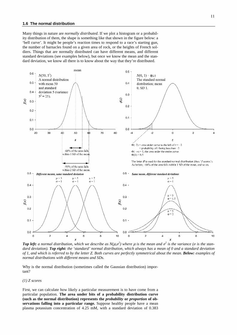
Many things in nature are normally distributed. If we plot a histogram or a probabil-ity distribution of them, the shape is something like that shown in the figure below: a‘bell curve’. It might be people’s reaction times to respond to a race’s starting gun,the number of barnacles found on a given area of rock, or the heights of French sol-diers. Things that are normally distributed can have different means, and differentstandard deviations (see examples below), but once we know the mean and the stan-dard deviation, we know all there is to know about the way that they’re distributed.

Top left: a normal distribution, which we describe as N(µ,σ2) where µ is the mean and σ2 is the variance (σ is the stan-dard deviation). Top right: the ‘standard’ normal distribution, which always has a mean of 0 and a standard deviationof 1, and which is referred to by the letter Z. Both curves are perfectly symmetrical about the mean. Below: examples ofnormal distributions with different means and SDs.

Why is the normal distribution (sometimes called the Gaussian distribution) impor-tant?

(1) Z scores

First, we can calculate how likely a particular measurement is to have come from aparticular population. The area under bits of a probability distribution curve(such as the normal distribution) represents the probability or proportion of ob-servations falling into a particular range. Suppose healthy people have a meanplasma potassium concentration of 4.25 mM, with a standard deviation of 0.383

12

mM, and that this is normally distributed. Since I’ve told you that about 95% of thepopulation fall within 2 SD of the mean, we can work out that 95% of healthy peo-ple have a potassium concentration in the range 3.5–5.0 mM. Furthermore, if a pa-tient has a potassium concentration of 5.5 mM, we can work out the probability ofthis concentration or higher being found in the healthy population. The way we dothat is as follows. It would be very tedious to work out the mathematical propertiesof the plasma-potassium normal distribution, which we’d call N(4.25, 0.3832),whenever we wanted to answer a question like this. It would certainly not be quickwith pen and paper. So we convert (‘transform’) our potassium score into a numberfrom N(4.25, 0.3832), which we know nothing about, to a special distribution calledthe standard normal distribution, which we write N(0,1) or Z, that we know eve-rything about. This is important and very easy: if x is our potassium measurement, µis our potassium mean, and σ is our potassium standard deviation, then

σµ−= x

z

In our example, z = (5.5 – 4.25)/0.383 = 3.26. We have converted our potassiumlevel of 5.5 mM to a Z score of 3.26. We can then use our tables of the standardnormal distribution (you’ve got a copy) to find out how likely a Z score of 3.26 (orhigher) is to have come from the standard normal distribution. This is answering thesame question as ‘how likely is a potassium level of 5.5 mM to have come from thedistribution of plasma potassium in healthy people?’ Our tables tell us that we wantthe probability that Z ≥ 3.26, and that’s 1 minus the probability that Z ≤ 3.26, whichis 0.9994; so the answer to our question is 1 – 0.9994 = 0.0006. In other words, it’shighly unlikely that a plasma potassium of 5.5 mM would be found in a healthypopulation. Our patient’s probably not healthy — better watch it, because if the po-tassium level goes too high, he’ll have a cardiac arrest.

Z scores carry information on their own, because you automatically know whatthe mean and standard deviation are (they’re 0 and 1, respectively).

Extreme Z scores (big positive numbers or big negative numbers) are unlikelyto have come from the distribution in question.

Sometimes, information is presented in a normalized form. For example, IQ scoresare transformed to a distribution with a mean of 100 and an SD of 15; knowing this,you can work out what proportion of the population have an IQ over 120.

(2) Assumptions of statistical tests

Second, many statistical tests assume that the data being tested is normally distrib-uted. We will return to this point later.

(3) Confidence intervals

Third, we can work out confidence intervals on any measurement we make. Wesaw an example above: we said that 95% of healthy people have a potassium con-centration in the range 3.5–5.0 mM. That is the same as saying the 95% confidenceinterval (CI) for the healthy-person data is 3.5–5.0 mM.

For any given set of data X, we can work out 95% confidence intervals as follows:1. Calculate the mean, µµµµ, and standard deviation, σ.2. The Z scores that enclose 95% of the population are –1.96 and +1.96. Why?

Well, our tables tell us that the area (probability) under the Z curve to the left ofz = –1.96, written, Φ(–1.96), is 0.025. Similarly, they tell us that Φ(+1.96) =0.975. Therefore the area under the normal curve between z = –1.96 and z =+1.96 is Φ(+1.96) – Φ(–1.96) = 0.95.

3. Z = (X – µ )/σ, therefore X = µ + Zσ. Therefore the X scores corresponding to Zscores of ±1.96 are µµµµ ± 1.96 σ, the 95% confidence intervals.

For our potassium example, we had a mean of 4.25 and an SD of 0.383; therefore,our 95% confidence intervals are 4.25 – (1.96 × 0. 383) and 4.25 + (1.96 × 0. 383),or 3.5 and 5.0. Try working out the 95% confidence intervals for IQ scores.

13

Deviations from normality

Not everything you measure will be normally distributed. Here’s a normal distribu-tion and some non-normal distributions:

Figures illustrating bimodality and skew.

Continuous random variables; probability density functions

(A-Level Further Maths.) For a continuous random variable X, the probability of anexact value x occurring is zero, so we must work with the probability density func-tion (PDF), f(x). This is defined as

dxxfbxaPb

a∫=≤≤ )()(

1)( =∫∞

∞−dxxf

0)(: ≥∀ xfx

( x∀ means ‘for all values of x’). The mean or expected value E[X] is defined as

dxxxfXE ∫=∞

∞−)(][

The variance, Var[X] is given by

22 ])[()(][ XEdxxfxXVar −∫=∞

∞−

The cumulative distribution function (CDF, also known as the ‘distribution function’or ‘cumulative density function’), F(a), is given by

dxxfaFa

∫=∞−

)()(

i.e.)()( axPaF ≤=

)()()( aFbFbxaP −=≤≤

Definition of a normal distribution

2

2

2

)(

2

1)( σ

µ

πσ

−−

=x

exf This distribution is often abbreviated to N(µ, σ2).

The standard normal distribution

The ‘standard’ normal distribution is N(0,1), i.e. a normal distribution in which µ =0 and σ = σ2 = 1. A standard normal random variable is frequently referred to as Z.The PDF is frequently referred to as )(zφ , and the CDF as )(zΦ . So

2

2

2

1)(

z

ez−

=π

φ ∫=Φ∞−

zdttz )()( φ

Transforming any normal distribution to the standard normal distribution

As we’ve seen, if X is a normally-distributed random variable with mean µ and stan-dard deviation σ, and Z is a standard normal random variable, then

σµ−= x

z

14

1.7 Probability

How much probability do you have to know? Not very much. You need to knowwhat a probability is, what P(A) and P(¬A) mean, and preferably what P(B|A)means. If you’re not keen on probability, you can skip the rest of this section andmove on to the logic of null hypothesis testing. If you’re a bit more capable mathe-matically, you may like to read this section — probability is at the heart of statisticaltesting and you’ll be streaks ahead of many researchers if you have a solid grasp ofprobabilistic reasoning.

Basic notation in probability

)(AP probability of an event A

)( AP ¬ probability of the event ‘not-A’, the opposite of A.

This is variously written as ¬A, ~A or A .)( BAP ∨ probability of A or B (or both) happening (the nota-

tion is like set union: ∪). Sometimes writtenP(A or B).

)( BAP ∧ probability of A and B both happening (the notationis like set intersection: ∩). Sometimes writtenP(A, B).

)|( ABP probability of B, given that A has already happened

Basic laws of probability

If P(A) = 0, then A will never happen (is impossible); if P(A) = 1, then A is certainto happen. Probabilities are always in this range:

0 ≤ P(A) ≤ 1 [1]

Pick a card; there are 52 equally-likely outcomes; 13 are clubs, so P(♣) = 13/52:P(A) = number of ways in which A occurs

number of ways in which all equally likely events, including A, occur[2]

Either A happens or ¬A happens (I flip a coin, it either comes up heads or tails):P(A) + P(¬A) = 1P(¬A) = 1 – P(A)

[3]

Odds

Odds are another way of expressing probability: they’re the ratio of P(A) to P(¬A).For example, Tiger Woods might be the favourite to win a tournament at odds of9:5, often stated ‘9 to 5 on’ (= 9/5 = 1.8). This means that for every 14 times heplays the tournament, he’d be expected to win 9 times and lose 5. If the event thatTiger Woods wins is A and his odds are x, we can write

xAP

AP =¬ )(

)(

Therefore

xAP

AP =− )(1

)(…

xAP

AP 1

)(

)(1 =−… )()( APAxPx =− … )()1( APxx += …

x

xAP

+=

1)(

So in the case of Tiger Woods, since x = 1.8, P(A) = 0.64. In general

odds

oddsyprobabilit

+=

1

If the odds on a player were quoted as ‘3 to 1 against’, the odds on them losing are3:1 so the odds on them winning are 1:3 (i.e. probability of them winning is ¼ =0.25).

15

The rest of the basic laws of probability

If A and B are mutually exclusive events (⇒ 0)( =∧ BAP ) then

)()()( BPAPBAP +=∨ [4]

In the more general case,)()()()( BAPBPAPBAP ∧−+=∨ [5]

If A and B are independent events — that is, the fact that A has happened doesn’taffect the likelihood that B will happen, and vice versa: )|()( ABPBP = and

)|()( BAPAP = — then

)()()( BPAPBAP ×=∧ [6]

If I toss a fair coin and roll a fair die, the probability of getting a six and a head is1/6 × 1/2 = 1/12. The probability of getting a six or a head or both is 1/6 + 1/2 – 1/12

= 7/12.

In the more general case:)|()()( ABPAPBAP ×=∧ [7]

If I have a bag that initially contains 4 red marbles and 6 blue marbles, and I with-draw marbles one by one, the probability of picking a red marble first (event A) anda blue marble second (event B) is 4/10 × 6/9 = 4/15.

A bit more advanced: Bayes’ theorem

From [7],

)(

)()|(

AP

BAPABP

∧=[8]

We also know, from [7],)|()()()( BAPBPABPBAP ×=∧=∧

Therefore, from [8],

)(

)|()()|(

AP

BAPBPABP

×=[9]

This is the simplest statement of Bayes’ theorem. Suppose event A is discoveringan improperly-sealed can at a canning factory. We know there are k assembly linesat which cans are sealed, and we’d like to know which one produced the faulty can.Let’s call B1 the event in which assembly line 1 produced the faulty can, B2 that inwhich line 2 produced the faulty can, and so on. What’s the probability that the cancame from line i?

We know that a faulty can must have came from one of the assembly lines:)|()(...)|()()|()()( 2211 kk BAPBPBAPBPBAPBPAP +++=

or to write that in a shorter form:

∑==

k

jjj BAPBPAP

1)|()()(

Therefore, from [9],

∑

×=

=

k

jjj

iii

BAPBP

BAPBPABP

1)|()(

)|()()|(

[10]

So suppose there are three assembly lines; lines X, Y and Z account for 50%, 30%and 20% of the total output. Quality control records show that line X produces 0.4%faulty cans, Y produces 0.6% faulty cans, and Z produces 1.2% faulty cans. UsingBayes’ theorem in the form of [10] will tell us that the chance our faulty can comesfrom line X is 0.32 (similarly, 0.29 for line Y and 0.39 for line Z).

16

Let’s take a simple, fictional example in which only two things may happen. Q. Theprevalence of a disease in the general population is 0.005 (0.5%). You have a bloodtest that detects the disease in 99% of cases: P(positive | disease) = 0.99. However, italso has a false-positive rate of 5%: P(positive | no disease) = 0.05. A patient ofyours tests positive. What is the probability he has the disease? A. We’d like to findP(disease | positive). By [9],

)|( posdisP

)(

)|()(

posP

disposPdisP ×=

)|()()|()(

)|()(

disposPdisPdisposPdisP

disposPdisP

¬¬+×=

05.0995.099.0005.0

99.0005.0

×+××=

= 0.09

So even though our test is pretty good and has a 99% true positive rate or ‘sensitiv-ity’ (a 1% false negative rate) and a 5% false positive rate (a 95% true negative rateor ‘specificity’), our positive-testing patient still only has a 9% chance of having thedisease — because it’s rare in the first place.

Bayesian inference

Suppose we have a hypothesis H. Initially, we believe it to be true with probabilityP(H); we therefore believe it to be false with probability P(¬H). We conduct an ex-periment that produces data D. We knew how likely D was to arise if H was true —P(D|H) — and we knew how likely D was to arise if H was false — P(D|¬H). Wecan therefore use Bayes’ theorem [9] to update our view of the probability of H:

)(

)|()()|(

DP

HDPHPDHP =

)|()()|()(

)|()()|(

HDPHPHDPHP

HDPHPDHP

¬¬+=

This can be expressed another way (Abelson, 1995, p. 42):

)|(

)|(

)(

)(

)|(

)|(

HDP

HDP

HP

HP

DHP

DHP

¬×

¬=

¬[11]

orposterior odds = prior odds × relative likelihood

17

1.8 The logic of null hypothesis testing; interpreting p values

We will come across a range of statistical tests. Most produce a test statistic and anassociated p value; you will see these quoted in scientific journals time and timeagain (F2,47 = 10.7, p < .001… F3,18 = 4.52, p = .016… t60 = 1.96, p = .055). They allwork on the same principle: that of null hypothesis testing.

Null hypothesis testing approaches the questions we want to ask backwards. Wetypically obtain some data. Let’s say we measure the weight of a hundred 18-year-old women who are either joggers (50) or non-joggers (50). We would like to knowwhether the mean weights of these two group differ. Obviously, it’s highly unlikelythat the means will be exactly the same. Suppose the joggers are slightly lighter onaverage. How big a difference counts as ‘significantly’ different? The conventionallogic is as follows. Either the difference arises through chance, or there is some sys-tematic difference (such as that jogging makes you thin, or that being thin encour-ages you to take up jogging). Our research hypothesis (sometimes written H1) isthat the joggers are different from the non-joggers (that our two samples come fromdifferent underlying populations). We’ll invent a corresponding null hypothesis(sometimes written H0) that the observed differences arise purely through chance.We’ll then test the likelihood that our data could have been obtained if this null hy-pothesis were true. If this probability (the so-called p value) is very low, we will re-ject the null hypothesis — chance processes don’t appear to be a sufficient explana-tion for our data, so something systematic must be going on; we’ll say that there is asignificant difference between our two groups. If the p value isn’t low enough, wewill retain the null hypothesis (applying Occam’s razor — because the null hy-pothesis is the simplest on offer) and say that the groups do not differ significantly.

The exact meaning of a p value

Let’s say we run a statistical test to examine whether these two groups differ. It pro-duces a test statistic (such as a t value; we’ll consider how this works later) and a pvalue — let’s say 0.01. What does this mean? For shorthand, let’s call D the event ofobtaining a set of data, H be the research hypothesis, and ¬H the null hypothesis.

• Correct: “If the null hypothesis were true [if it were true that there were nosystematic difference between the means in the populations from which thesamples came], the probability that the observed means would have been asdifferent as they were, or more different, is 0.01. This being strong groundsfor doubting the viability of the null hypothesis, the null hypothesis is re-jected.”

• Correct: P(D | ¬H) = 0.01.• Wrong: “The probability that the null hypothesis is true is 0.01.”• Wrong: “The probability that the research hypothesis is false is 0.01.”• Wrong: P(¬H | D) = 0.01.• Wrong: “The probability that the null hypothesis is false is 0.99.”• Wrong: “The probability that the research hypothesis is true is 0.99.”• Wrong: P(H | D) = 0.99.

It’s easy to think that these are all saying the same thing, but they’re not. Compare(1) the probability of testing positive for a very rare disease if you have it, P(positive| diseased), with (2) the probability of having it if you test positive for it, P(diseased |positive). If you think the two should be the same, you’re neglecting the ‘base rates’of the disease: typically, the second probability is less than the first, as it’s very un-likely for anybody to have a very rare disease, even those who test positive. Doctorsintuitively get this wrong all the time. Substitute in P(rich | won the lottery) andP(won the lottery | rich)… the first probability is much higher, because winning thelottery is so rare.

Bayes’ theorem and Bayesian statistics

The formal way to relate what we get from significance tests, P(data | ¬hypothesis),to what we really want, P(hypothesis | data), is by using Bayes’ theorem (see sectionon probability). This is perhaps the simplest expression to use in this case:

18

)|(

)|(

)(

)(

)|(

)|(

HDP

HDP

HP

HP

DHP

DHP

¬×

¬=

¬posterior odds = prior odds × relative likelihood.

For example, suppose that a climatologist calculates that a 1°C rise in temperatureone summer had a probability of 0.01 of occurring by chance (p = 0.01). What doesthat tell us? It does not tell us that there’s a 99% probability that it was due to thegreenhouse effect. It does not even tell us that there’s a 99% probability that it wasnot due to chance. The Bayesian approach would be this: suppose that reasonablepeople believed the odds were 2:1 in favour of the greenhouse hypothesis (H) beforethis new evidence was collected — these are the prior odds. Now, we’ve been toldthat P(D|¬H) = 0.01. We need to know the probability that a 1°C temperature risewould occur if the greenhouse hypothesis were true; that is, P(D|H). Suppose this is0.03. Then the relative likelihood is 0.03/0.01 = 3. So the posterior odds are 2 × 3 =6 in favour of the greenhouse hypothesis; odds of 6:1 equate to P(H|D) = 6/7 = 0.86.

Type I and Type II error; power

Although p values speak for themselves in one sense, it’s very common for re-searchers to use them as a yes/no decision-making device. I won’t debate the wis-dom of this now, but this is how it works. A threshold probability, usually called α(alpha), is chosen; typically, α = 0.05. If a given p value is less than α, the null hy-pothesis is rejected; if p ≥ α, the null hypothesis is retained. You might see this logicdescribed in papers like this: ‘the two groups were significantly different (p < 0.05),’or ‘a significance level of α = 0.05 was adopted throughout our study… the twogroups were significantly different.’

Obviously, if α = 0.05, then there is a 0.05 (one in twenty) chance that an effect welabel as ‘significant’ could have arisen by chance if the null hypothesis was true. Ifthis happens, and we accidentally decide that a effect was not attributable to chancewhen actually it did arise by chance, we’re said to have made a Type I error. Theprobability of making a Type I error is α. Conversely, the probability of correctlynot rejecting the null hypothesis when it is true is 1 – α.

The opposite mistake is failing to reject the null hypothesis when it is false — thatis, ascribing your data to chance when it actually arose from a systematic effect.This is called a Type II error; its probability is labelled β (beta). Conversely, theprobability of correctly rejecting the null hypothesis when it is in fact false is 1 – β;this is called the power of the test. If your power is 0.8, it means that you will detect‘genuine’ effects with p = 0.8.

True state of the worldDecision H0 true H0 falseReject H0 Type I error

p = αCorrect decisionp = 1 – β = power

Do not reject H0 Correct decisionp = 1 – α

Type II errorp = β

One-tailed and two-tailed tests

There’s one other thing we should consider when we talk about α and Type I error.Let’s go back to the example of our joggers. Presumably our leading hypothesis isthat joggers will be thinner than non-joggers, so we want to be able to detect if themean weight of joggers is less than that of non-joggers, and we might choose α =0.05. But what will we do if the joggers actually weigh more? Well, this depends onwhat kind of test we decided on. If we were only interested in the difference be-tween the groups if the joggers weighed less, we would use a one-tailed (direc-tional) test, so that if there was less than a 5% probability that chance alone couldhave produced a difference in the direction we expect then we would reject the nullhypothesis. But if we want to be able to detect a difference in either direction, wemust use a two-tailed (nondirectional) test. In that case, we must ‘allocate’ our 5%

19

α to the two ways in which we could find a difference (joggers weigh more; joggersweigh less) — so we’d allocate 2.5% to each tail of the distribution. This is shownin the figure below (plotted on a normal distribution; you might like to think of it interms of the joggers and the potassium examples). In general, unless you wouldgenuinely not be interested in both possible outcomes (quite a rare situation), youshould use a two-tailed test. What you must not do is to run a one-tailed test (α =0.05), find a non-significant result, then look at the data, realize the difference is inthe other direction to the one you predicted, and decide then to do a two-tailed test(α = 0.05) — because what you have actually done is to allocate 5% to one tail, thenallocate another 2.5% to the other tail, meaning that you have actually run a sort ofasymmetric two-tailed test with a total α of 0.075 (7.5%). Decide what test you wantin advance of analysing the data.

One-tailed and two-tailed tests.

The danger of running multiple significance tests

Every time you run a test, if the null hypothesis is true, you run the risk of making aType I error with probability α. So if you run n tests, you have n chances to make aType I error. What’s the probability that you don’t make any Type I errors when yourun n tests? Well, the probability that you don’t make a Type I error on each test is 1– α, so the probability you make no Type I errors when you run n tests is (1 – α)n. Sothe probability that you make at least one Type I error when you run n tests whenthe null hypothesis is true is 1 – (1 – α)n.

If you set α = 0.05, you must expect on average one in every 20 tests to come up‘significant’ when it isn’t (Type I error) if the null hypothesis is in fact true. If yourun 20 tests and the null hypothesis is true, the probability of making at least oneType I error is 1 – (1 – 0.05)20 = 0.64. This is why running lots of tests willy-nilly isa Bad Idea — eventually, something will ‘turn up significant’, but that doesn’t meanit really is.

This doesn’t mean that 5% of all your significant results are ‘wrong’. You can onlymake Type I errors when the null hypothesis is true! In practice, on some occasionsthe null hypothesis will be false, so we can’t make a Type I error. Therefore, some-thing less than 5% of our ‘significant’ results will be Type I errors; α is the maxi-mum Type I error rate.

Is there a difference between p = 0.04 and p = 0.0001?

Yes. Whether you look on p values as expressing the degree of confidence withwhich you reject the null hypothesis, or as information you can use to update youropinions of the world in Bayesian fashion, p values have real meaning. Some peoplewill argue that as long as p < α you needn’t report the actual p value, but this ap-proach takes information away from the reader.

p = 0.06

20

What happens if you run a well-designed experiment in which you give a treatmentto one group of people and not another, measure some aspect of their performance,test for a difference between your groups and get p = 0.06? You could do one ofseveral things. (1) Re-run your experiment with more subjects; perhaps you did nothave enough statistical power to detect the size of effect that your treatment pro-duced. You might have been spared this embarrassment if you had tried to calculateyour statistical power in advance; you might then have realised your experiment wasunder-powered in the first place. (2) Report your experiment as showing a ‘trend’towards an effect; it’s not like p = 0.04 is somehow magically better than p = 0.06,after all. (3) Use α = 0.1 rather than α = 0.05. However, not only will journal editorsdefinitely be upset with this (for no real reason — there’s nothing magical about α =0.05), but it is highly dubious to change your α only after you’ve run your experi-ment — after all, you’re only doing it to shore up a not-quite-significant result, andyou’re therefore distorting the results. You should have chosen α in advance. Simi-larly, it is very dubious to add subjects to your original experiment ‘until it reachessignificance’ — you’re only doing this because your original data was ‘near’ signifi-cance and you want it to be significant. If you had a compelling reason to want yourtreatment to have no effect, you wouldn’t be doing this — so you’re biasing the ex-periment by this kind of post-hoc fiddling.

What does ‘not significant’ mean?

What happens when you want to prove that a hypothesis is not true? Suppose yourcontention is that jogging doesn’t affect body weight; you take two identical groupsof people, set half of them jogging for a couple of months while the rest eat pies, andmeasure their weights. You find no difference between the groups (p = 0.12). Whatdoes this mean? It means that you have failed to reject the null hypothesis — there isa fair chance (0.12) that your observed difference could have arisen by chance alone.It does not mean that you have proven the null hypothesis. Take an extreme exam-ple: your null hypothesis is that all people have two arms. Just because the next5,000 people you meet all have two arms (failure to reject the null hypothesis) doesnot mean that you have proved the null hypothesis.

You can do two things when you fail to reject the null hypothesis: (1) view it as aninconclusive result, or (2) act as if the null hypothesis were true until further evi-dence comes along.

Really, you should consider your level of α and β to meet the needs of your study. Ifyou want to avoid Type I errors (e.g. telling someone they have an ulcer when theydon’t), set α low. If you want to avoid Type II errors (e.g. telling them to go homeand rest when they’re about to die from a gastric haemorrhage), set α higher. Theother thing you can do when you’re designing an experiment is to make sure thepower is high enough to detect effects with a reasonable probability — such as byusing enough subjects. If you take two people and make one jog, you’ll never find a‘significant’ difference between the jogging and non-jogging groups, but thatdoesn’t mean people should believe you when you say that jogging doesn’t reduceweight. If you used half a million people and still found no effect, your study mightcommand more attention.

A statistical fallacy to avoid: A differs from C, B doesn’t differ from C…

If you test three groups and find that A is significantly different from C, but B is notsignificantly different from C, do not conclude that A is significantly different fromB. To see why, imagine that A is smaller than B, and B is smaller than C. Then wemight find a difference between A and C (p = 0.04) and no difference between Band C (p = 0.06) — but the p values are just on either side of our threshold of 0.05and A and B might be nearly the same! Making this conceptual mistake is quitecommon.

Similarly, just because A isn’t significantly different from B, and B isn’t signifi-cantly different from C, doesn’t mean that A isn’t significantly different from C.

21

1.9. For future reference…

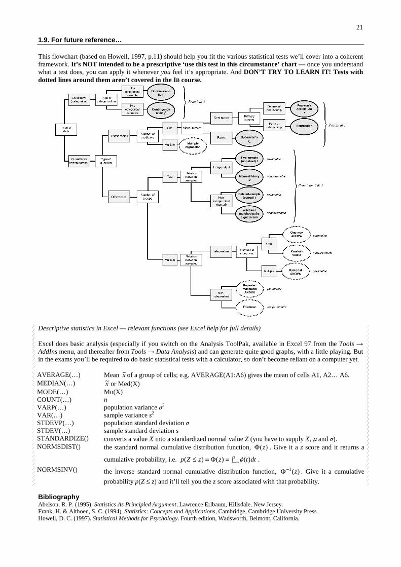
This flowchart (based on Howell, 1997, p.11) should help you fit the various statistical tests we’ll cover into a coherentframework. It’s NOT intended to be a prescriptive ‘use this test in this circumstance’ chart — once you understandwhat a test does, you can apply it whenever you feel it’s appropriate. And DON’T TRY TO LEARN IT! Tests withdotted lines around them aren’t covered in the IB course.

Descriptive statistics in Excel — relevant functions (see Excel help for full details)

Excel does basic analysis (especially if you switch on the Analysis ToolPak, available in Excel 97 from the Tools →AddIns menu, and thereafter from Tools → Data Analysis) and can generate quite good graphs, with a little playing. Butin the exams you’ll be required to do basic statistical tests with a calculator, so don’t become reliant on a computer yet.

AVERAGE(…) Mean x of a group of cells; e.g. AVERAGE(A1:A6) gives the mean of cells A1, A2… A6.MEDIAN(…) x~ or Med(X)MODE(…) Mo(X)COUNT(…) nVARP(…) population variance σ2

VAR(…) sample variance s2

STDEVP(…) population standard deviation σSTDEV(…) sample standard deviation sSTANDARDIZE() converts a value X into a standardized normal value Z (you have to supply X, µ and σ).NORMSDIST() the standard normal cumulative distribution function, )(zΦ . Give it a z score and it returns a

cumulative probability, i.e. ∫=Φ=≤ ∞−z dttzzZp )()()( φ .

NORMSINV() the inverse standard normal cumulative distribution function, )(1 z−Φ . Give it a cumulative

probability p(Z ≤ z) and it’ll tell you the z score associated with that probability.

BibliographyAbelson, R. P. (1995). Statistics As Principled Argument, Lawrence Erlbaum, Hillsdale, New Jersey.Frank, H. & Althoen, S. C. (1994). Statistics: Concepts and Applications, Cambridge, Cambridge University Press.Howell, D. C. (1997). Statistical Methods for Psychology. Fourth edition, Wadsworth, Belmont, California.