Page 1
Status of Numerical Relativity:From my personal point of view
1 Introduction2 General issues in numerical relativity3 Current status of implementation4 Some of our latest numerical results:
NS-NS merger & Stellar core collapse5 Summary & perspective
Masaru Shibata (U. Tokyo)
Page 2
1: Introduction: Roles in NRA To predict gravitational waveforms:
Two types of gravitational-wave detectors work now or soon.
Frequency
h
0.1mHz 0.1Hz 10Hz 1kHz
LISA LIGO/VIRGO/GEO/TAMA
Space Interferometer Ground Interferometer
Templates (for compact binaries, core collapse, etc) should be prepared
Physics of SMBH
SMBH/SMBHBH-BHNS-NS
SN
Page 3
B To simulate Astrophysical Phenomenae.g. Central engine of GRBs
= Stellar-mass black hole + disks (Probably)
NS-NS merger
BH-NS merger
Stellar collapse of rapidly rotating star
Best theoretical approach= Simulation in GR
?
Page 4
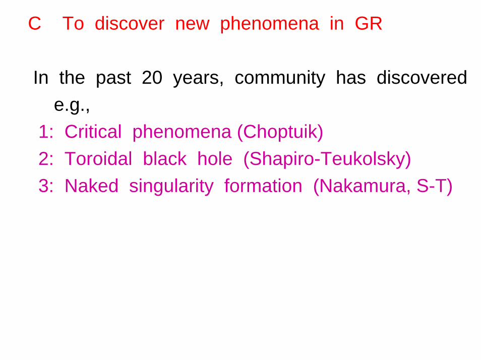
C To discover new phenomena in GR
In the past 20 years, community has discovered e.g.,
1: Critical phenomena (Choptuik)2: Toroidal black hole (Shapiro-Teukolsky)3: Naked singularity formation (Nakamura, S-T)
Page 5
GR phenomena to be simulated ASAP
・ NS-NS / BH-NS /BH-BH mergers (Promising GW sources/GRB)
・ Stellar collapse of massive star to a NS/BH (Promising GW sources/GRB)
・ Nonaxisymmetric dynamical instabilities of rotating NSs
(Promising GW sources)・ ….
In general, 3D simulations are necessary
Page 6
2 Issues: Necessary elements for GR simulations
• Einstein’s evolution equations solver• GR Hydrodynamic equations solver• Appropriate gauge conditions (coordinate conditions)• Realistic initial conditions in GR• Gravitational wave extraction techniques• Apparent horizon (hopefully Event horizon) finder• Special techniques for handling BHs / BH excision• Micro physics (EOS, neutrino processes, B-field …)• Powerful supercomputers
RED = Indispensable elements
Page 7
3: Current Status: Achievements in the past decade
• Einstein evolution equation solver in 3D
• GR Hydro equation solver
• Appropriate gauge conditions in 3D
• Supercomputers
Here, focus on progress in main elements:
Page 8
Progress I • Formulations for Einstein’s evolution equation
Many people 10 yrs ago believed the standard ADM formalism works well. BUT:
Numerical simulationbecomes unstableeven in the evolution of
linear GW(Nakamura 87, Shibata 95, Baumgarte-Shapiro (99)12 components
Due to constraint violation instabilities
Unconstrainedfree evolution
Standard ADMVariables in standard ADM formalism: , ij ijKγ
Page 9
• New formulations for Einstein’s evolution eqs :(i) BSSN formalism
Stable numerical simulation(So far no problem in theabsence of black holes)
( )4
4
Choose variables:1 ln det( )
12
13
ij ij
kk
ij ij ij
jki j ik
e
K K
A e K K
F
φ
φ
φ γ
γ γ
γ
δ γ
−
−
≡
≡
≡
≡ −
≡ ∂17 components
Nakamura (87), Shibata-Nakamura (95), Baumgarte-Shapiro (99)…..
Unconstrainedfree evolution
An Important step
( )
Rewrite ADM equations using
det 1ij
constraint equations
γ
=
Page 10
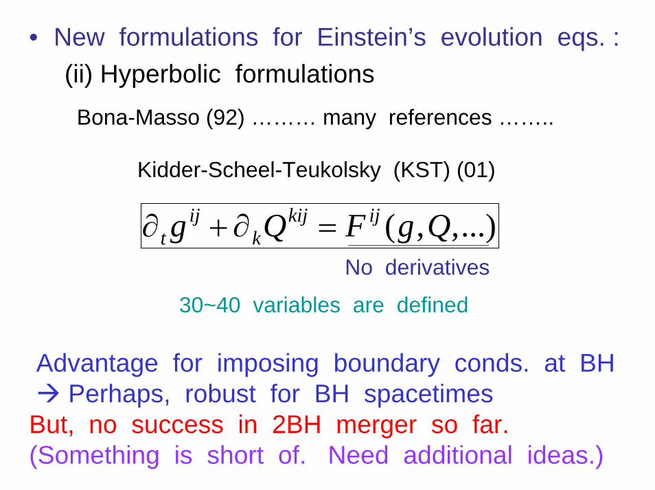
• New formulations for Einstein’s evolution eqs. :(ii) Hyperbolic formulations
Bona-Masso (92) ……… many references ……..
Kidder-Scheel-Teukolsky (KST) (01)
Advantage for imposing boundary conds. at BHPerhaps, robust for BH spacetimes
But, no success in 2BH merger so far.(Something is short of. Need additional ideas.)
No derivatives
( , ,...)ij kij ijt kg Q F g Q∂ + ∂ =
30~40 variables are defined
Page 11
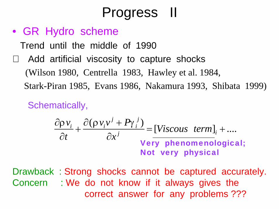
Progress II• GR Hydro scheme
Trend until the middle of 1990⇒ Add artificial viscosity to capture shocks
(Wilson 1980, Centrella 1983, Hawley et al. 1984, Stark-Piran 1985, Evans 1986, Nakamura 1993, Shibata 1999)
Drawback : Strong shocks cannot be captured accurately.Concern : We do not know if it always gives the
correct answer for any problems ???
Schematically,
( ) [ ] ....j j
i i iij
v v v P Viscous termt xρ ρ γ∂ ∂ +
+ = +∂ ∂
Very phenomenological;Not very physical
Page 12
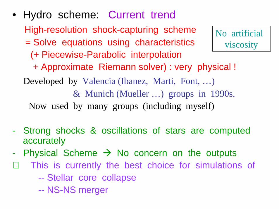
• Hydro scheme: Current trendHigh-resolution shock-capturing scheme= Solve equations using characteristics(+ Piecewise-Parabolic interpolation+ Approximate Riemann solver) : very physical !
Developed by Valencia (Ibanez, Marti, Font, …) & Munich (Mueller …) groups in 1990s.
Now used by many groups (including myself)
- Strong shocks & oscillations of stars are computed accurately
- Physical Scheme No concern on the outputs⇒ This is currently the best choice for simulations of
-- Stellar core collapse-- NS-NS merger
No artificial viscosity
Page 13
Standard tests for hydro code in special relativity
V = 0.9c.N = 400, Γ = 4/3
Riemann Shock Tube Wall ShockN = 400, Γ = 5/3
P1 > P2ρ1 > ρ2 V -V
Density
Pressure
Velocity
Page 14
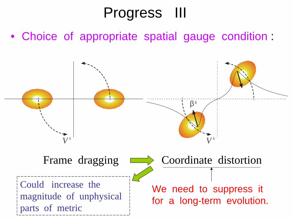
Progress III• Choice of appropriate spatial gauge condition :
V k
β k
V k
Frame dragging Coordinate distortion
We need to suppress it for a long-term evolution.
Could increase the magnitude of unphysical parts of metric
Page 15
γxx on the equatorial planewith zero shift vector
t=12.9
t=0.0 t=4.8
t=8.7
1 2 at ~2xxPtγ − ≈
T=0 T~P/6
T~P/3
Distortion monotonically increases to crash
diverge
Page 16
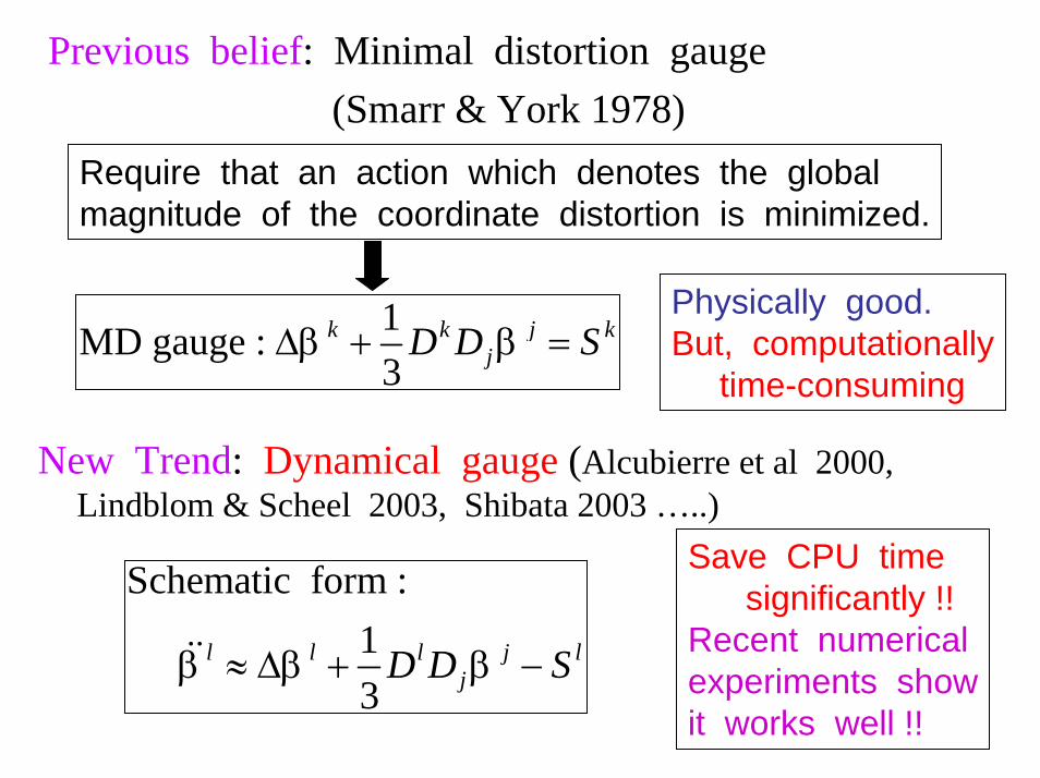
Previous belief: Minimal distortion gauge (Smarr & York 1978)
New Trend: Dynamical gauge (Alcubierre et al 2000, Lindblom & Scheel 2003, Shibata 2003 …..)
Save CPU timesignificantly !!
Recent numerical experiments showit works well !!
Physically good.But, computationally
time-consuming
1MD gauge : 3
k k j kjD D Sβ β∆ + =
Schematic form : 1 3
l l l j ljD D Sβ β β≈ ∆ + −
Require that an action which denotes the global magnitude of the coordinate distortion is minimized.
Page 17
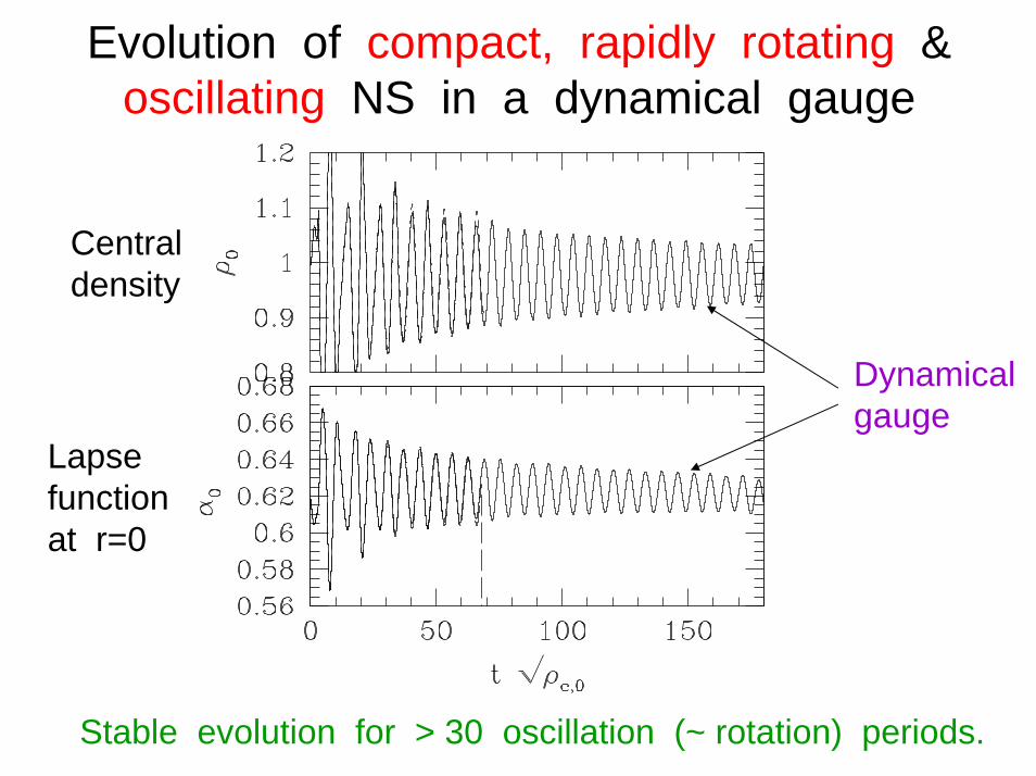
Evolution of compact, rapidly rotating & oscillating NS in a dynamical gauge
Centraldensity
Lapsefunctionat r=0
Dynamicalgauge
Stable evolution for > 30 oscillation (~ rotation) periods.
Page 18
L >> r
rTotal mass M
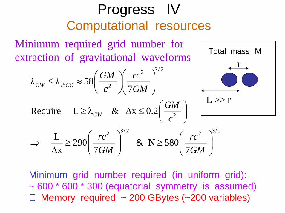
Progress IVComputational resources
Minimum required grid number for extraction of gravitational waveforms
Minimum grid number required (in uniform grid): ~ 600 * 600 * 300 (equatorial symmetry is assumed)⇒ Memory required ~ 200 GBytes (~200 variables)
3/ 22
2
2
3/ 2 3/ 22 2
587
Require L & x 0.2
L 290 & N 580x 7 7
GW ISCO
GW
GM rcc GM
GMc
rc rcGM GM
λ λ
λ
≤ ≈
≥ ∆ ≤
⇒ ≥ ≥ ∆
Page 19
An example of current supercomputer
• Vector-Parallel Machine (60 vector PEs)• Maximum memory 0.96TBytes• Maximum speed 0.58TFlops• Our typical run with 32PEs
633 * 633 * 317 grid points = 240 Gbytes memory(in my code)
About 20,000 time steps ~ 100 CPU hours /model
FUJITSU FACOM VPP5000 at NAOJ
Minimum grid number can be taken
But, hopefully, we need hypercomputersfor well-resolved simulations.
(e.g. Earth simulator ~ 10TBytes, ~ 40TFlops)
Typical current memory & speed
Page 20
Summary of current statusOKOKOK
~OKbut hopefully need hypercomputers
• Einstein evolution equations solver• Gauge conditions (coordinate conditions)• GR Hydrodynamic equations solver• Powerful supercomputer
Long-term GR simulations are feasible (in the absence of BHs)
In the past 5 yrs, computations have been done for・ NS-NS merger (Shibata-Uryu, Miller, …)・ Stellar core collapse (Font, Papadopoulas, Mueller, Shibata)・ Collapse of supermassive star (Shibata-Shapiro)・ Bar-instabilities of NSs (Shibata-Baumgarte-Shapiro)・ Oscillation of NSs (Shibata, Font-Stergioulas, ….)
Page 21
Unsolved Issue : Handling BHs
Time has to bestopped proceeding
Time proceedsoutside BH
α
Lapse
R
Gradient istoo large
Accurate computationbecomes difficult
Horizon
BH
0
Page 22
A solution = Excision(Unruh)
What are appropriate formulation, gauge, boundary conditions …. ?
-- 1BH OK (Cornell, Potsdam, Illinois…)-- 2BH No success for a longterm simulation(But see gr-qc/0312112, Bruegmann et al. for one orbit)
ApparentHorizon
Excision
No pointsinside
Page 23
4. Our latest numerical results:Current implementation in our group
1. GR : BSSN (or Nakamura-Shibata). But modified year by year; e.g., latest version = Shibata et al. 2003 has improved accuracy significantly
2. Gauge : Maximal slicing (K=0) + Dynamical gauge
3. Hydro : High-resolution shock-capturing scheme(Roe-type method with 3rd-order PPM interpolation)
Page 24
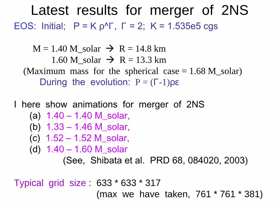
Latest results for merger of 2NSEOS: Initial; P = K ρ^Γ, Γ = 2; K = 1.535e5 cgs
M = 1.40 M_solar R = 14.8 km1.60 M_solar R = 13.3 km
(Maximum mass for the spherical case = 1.68 M_solar)During the evolution: P = (Γ-1)ρε
I here show animations for merger of 2NS(a) 1.40 – 1.40 M_solar, (b) 1.33 – 1.46 M_solar,(c) 1.52 – 1.52 M_solar, (d) 1.40 – 1.60 M_solar
(See, Shibata et al. PRD 68, 084020, 2003)
Typical grid size : 633 * 633 * 317 (max we have taken, 761 * 761 * 381)
Page 25
Evolution of maximum density in NS formation
Oscillating hypermassiveneutron starsare formed
Unequal mass1.33—1.46
Equal mass1.40—1.40
Not crash.We artificially stopped simulation.
Page 26
1.40 – 1.40 M_solar case : final snapshotMassive toroidal neutron star is formed
(slightly elliptical)
X – Y contour plot X – Z contour plot
Toroidal shape
Page 27
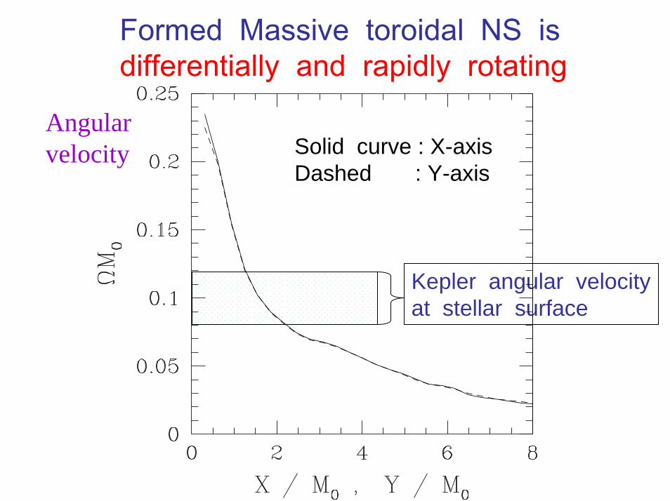
Kepler angular velocity at stellar surface
Formed Massive toroidal NS is differentially and rapidly rotating
Angularvelocity Solid curve : X-axis
Dashed : Y-axis
Page 28
1.33—1.46: Massive NS + disk
Unequal-mass caseMass ratio ~ 0.90
Equal-mass case
1.40—1.40: Massive NS
Comparison between equal and unequal mass mergers
Page 29
Black hole formation case: 1.52-1.52Equal-mass case
Apparent horizon
Mass for r > 3M~ 0.2%
Page 30
Disk mass for unequal-mass merger
Mass for r > 3M~ 4%
1.45—1.55, Mass ratio 0.925 1.40—1.60, Mass ratio 0.855
Mass for r > 3M~ 2%
Page 31
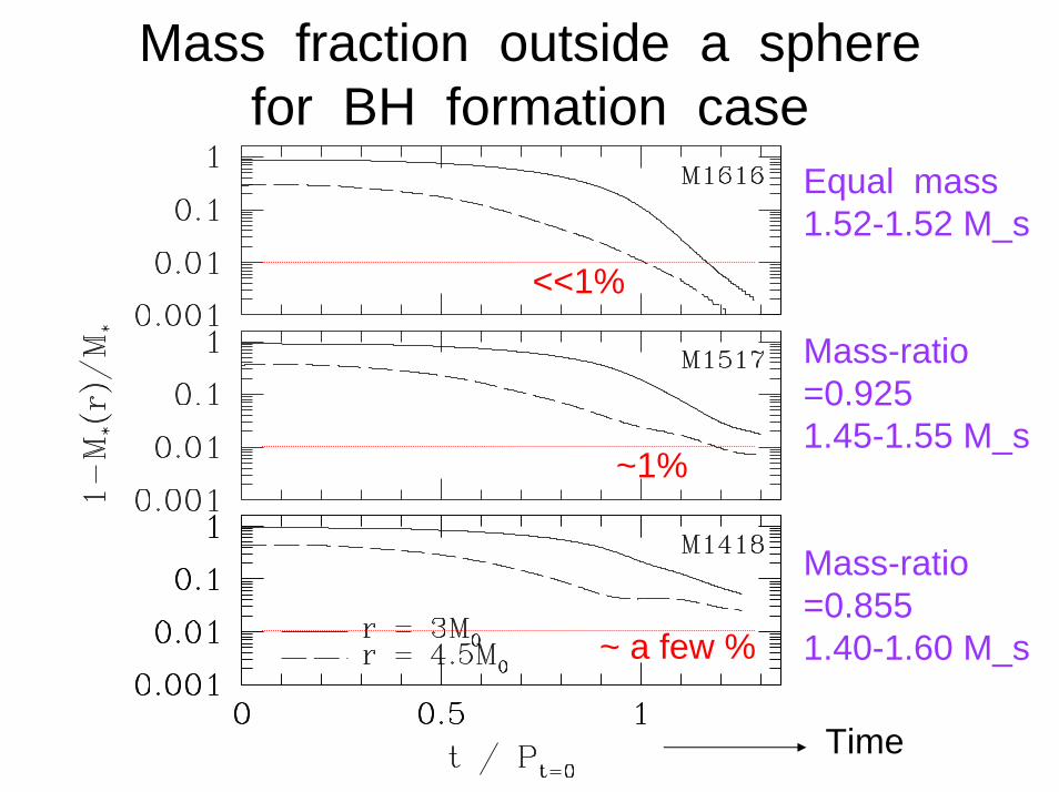
Mass fraction outside a spherefor BH formation case
Equal mass1.52-1.52 M_s
Mass-ratio=0.9251.45-1.55 M_s
Mass-ratio=0.8551.40-1.60 M_s
<<1%
~1%
~ a few %
Time
Page 32
Products of mergers for Γ = 2
Equal – mass cases・ Low mass cases
Hypermassive neutron starsof nonaxisymmetric & quasiradial oscillations.
・ High mass casesDirect formation of Black holes
with very small disk mass
Unequal – mass cases (mass ratio ~ 0.9)・ Likely to form disks of mass
~ several percents of total massBH(NS) + Disk (~0.1M_solar) Maybe a candidate for short GRB
Page 33
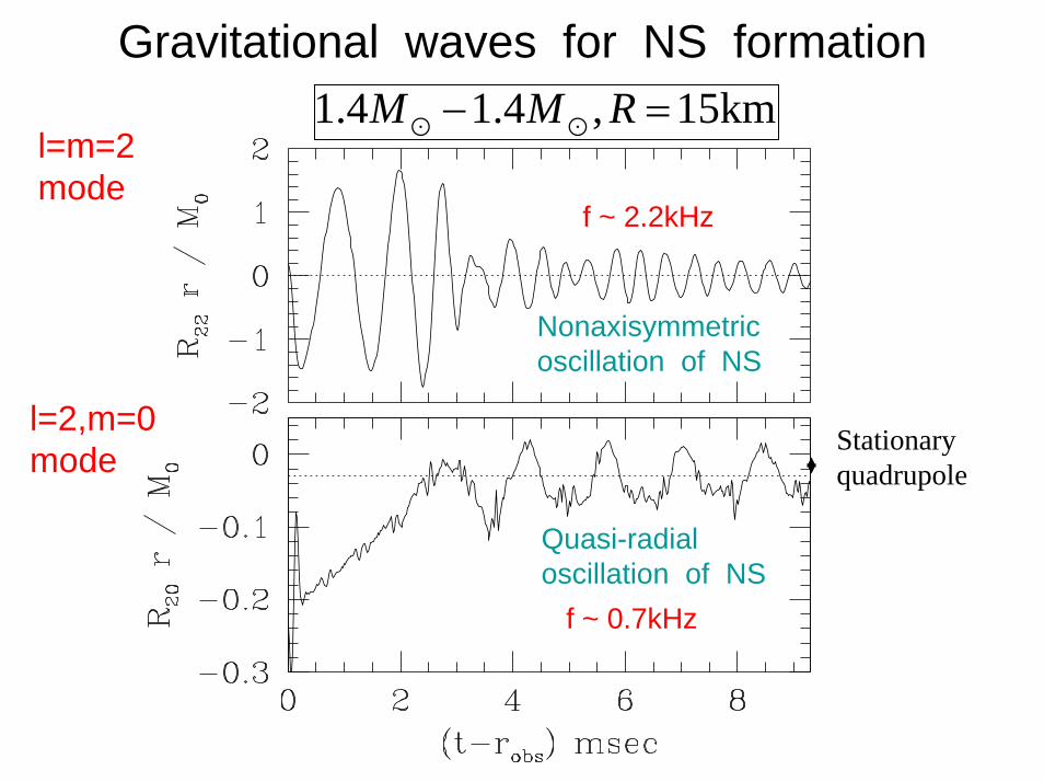
Gravitational waves for NS formation
l=m=2 mode
1.4 1.4 , 15kmM M R− =
l=2,m=0 mode
Nonaxisymmetricoscillation of NS
Quasi-radial oscillation of NS
f ~ 0.7kHz
f ~ 2.2kHz
Stationaryquadrupole
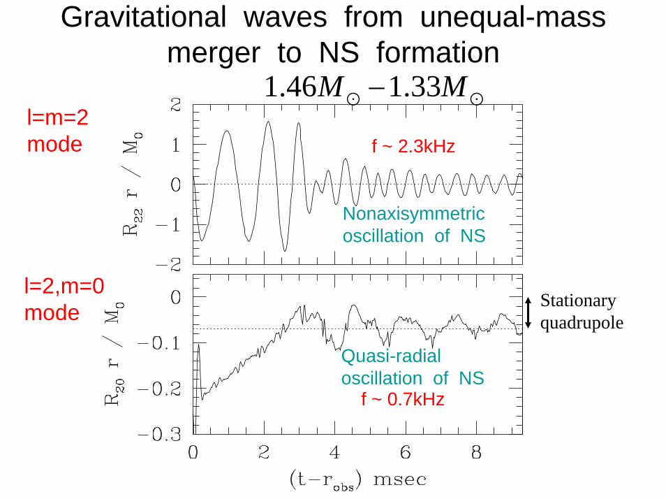
Page 34
Gravitational waves from unequal-massmerger to NS formation
l=m=2 mode
l=2,m=0 mode
Nonaxisymmetricoscillation of NS
Quasi-radial oscillation of NS
f ~ 0.7kHz
f ~ 2.3kHz
1.46 1.33M M−
Stationaryquadrupole
Page 35
Fourier spectrum in NS formation~2.2kHz (equal mass)
~2.3kHz (unequal massMass ratio=0.9)
Inspiral wave
~(dE/df)^{1/2}
Frequencyalso dependson EOS.~0.7kHz
Non-axisym.oscillation
Quasi-radialoscillation
Page 36
Computation of mass and angular momentum-- Check of the conservation --
Computational domain
Whole regionM=M0J=J0
M’, J’
M0-EGW=M’ & J0-JGW=J’should be satisfied
GW GW
EGW
Local wavezone
Page 37
Radiation reaction : OK within ~ 1%NS formation: equal mass BH formation: unequal mass
Solid curves : computed from data sets in finite domain.Dotted curves: computed from fluxes of gravitational waves
Mass energy
Angular mom.
Mass energy
Angular mom.
BHformation
M’M0-∆E
J0-∆J
J’
Page 38
5 Summary
1 Rapid progress in particular in the past 5 yrs2 Scientific (quantitative) runs are feasible now.3 (Astrophysically) Accurate and longterm
simulations are feasible for many phenomena in the absence of BHs : NS-NS merger, Stellar collapse, Bar-instabilities of NSs ….
4 (I think) numerical implementations for fundamental parts have been almost established (for the BH-absent spacetimes)
Page 39
Issues for the near future 1 Several (technical) Issues still remain :・ Grid numbers are still not large enough in 3D
We would need hypercomputer (~10TBytes, ~10TFlops)
Probably becomes available in a couple of yrs. ・ Computation crashed due to grid stretching
around BH horizon We need to develop excision techniques.
・ How to achieve a very high accuracy for making GW templates ?
2 Incorporate more realistic physics in hydro simualtion
More realistic EOS, Neutrino cooling, Magnetic fields
Page 40
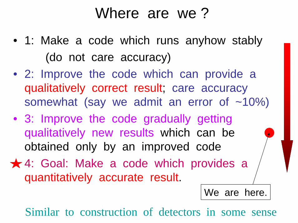
Where are we ?
• 1: Make a code which runs anyhow stably (do not care accuracy)
• 2: Improve the code which can provide aqualitatively correct result; care accuracy somewhat (say we admit an error of ~10%)
• 3: Improve the code gradually getting qualitatively new results which can be obtained only by an improved code
• 4: Goal: Make a code which provides aquantitatively accurate result.
We are here.
Similar to construction of detectors in some sense
Page 41
Animations• http://esa.c.u-tokyo.ac.jp/~shibata/anim.html