UCLEAR PHYSIC~

PROCEEDINGS SUPPLEMENTS

FJSEVIER Nuclear Physics B (Proc. Suppl,) 47 (1996) 473-480

Status Report on Weak Matrix Element Calculations*

Rajan Gupta and Tanmoy Bhattaz~harya ~

aT-8 Group, MS B285, Los Alamos National Laboratory, Los Alamos, New Mexico 87545 U. S. A.

This talk presents results of weak matrix elements calculated from simulations done on 170 32 a x 64 lattices at ~ = 6.0 using quenched Wilson fermioas. We discuss the extraction of pseudoscalar decay constants f~, fK, ]D, and ]Do, the form-factors for the rare decay B -~ K*7, and the matrix elements of the 4-fermion operators relevant to BK, B,, Bs. We present an analysis of the various sources of systematic errors, and show that these are now much larger than the statistical errors for each of these observables. Our main results arc fD = 186(29) MeV, fD° = 224(16)MeV, 7"1 = T2 = 0.24(1), BK(NDR, 2 GeV) = 0.67(9), and B,(NDR, 2 GeV) = 0.81(1).

1. T E C H N I C A L D E T A I L S

We briefly state the details common to all three quantities discussed in this talk and refer the reader to [1, 2, 3] for details. Preliminary re- sults based on 100 lattices were presented at LAT- TICE94 [4l and the final analysis will be pre- sented elsewhere [2, 5].

We calculate wall and Wuppertal source quark propagators at five values of quark mass given by

= 0.135 (C), 0.153 (S), 0.155 (0"1), 0.1558 (U2), and 0.1563 (U3). These quarks correspond to pseudoscalar mesons of mass 2835, 983, 690, 545 and 431 MeV respectively where we have used 1/a = 2.33 GeV for the lattice scale. We con- struct three types of correlation functions, Wup- pertal smeared-local (FsL) and smeared-smeared (Fss) , and wall smeared-local (FwL). The three Ui quarks allow us to extrapolate the data to the physical isospin symmetric light quark mass

= (mu + rod)~2, while the physical charm mass is taken to be C. The physical value of strange quark lies between S and U1 and we use these two points to interpolate to it. For brevity we will denote the six combinations of light quarks U1U1, U1U2, U1Us, U2U2, U2Ua, U3Us by {U~Ui} and the three degenerate cases by {UiUi}. The FsL, Fss, and 3-point functions have been evaluated at the 5 lowest lattice momenta, i.e. p= (0,0,0), (1, 0, 0), (1, 1, 0), 0 , 1 , 1 ) , (2, 0, 0 ).

* Based on talks presented by Rajah Gupta and ~ m m o y Bhattacharya. These calculations have been done on the CM5 at LANL as part of the DOE HPCC Grand Challenge program, and at NCSA under a Metacenter allocation.

1996 Elsevier Science B.V. PII: S0920-5632(96)00104- l

Renormallzation Constants: We use the Lepage-Mackenzie tadpole subtraction prescrip- tion [6]. Its implementation consists of three parts in addition to writing the perturbat ive ex- pansions in terms of the improved coupling av. One, the renormalization of the quark field v ~ ¢

changes from ~ -~ 8v~cy/1 - 3~/4~c; second, the perturbat ive expression for 8Ke in Z¢ is com- bined with the coefficient of av in the one loop matching relations to remove the tadpole contri- bution, and finally the typical momentum scale once the tadpole diagrams are removed is taken to be q* = 1/a, i.e. both the scale at which av is evaluated and the scale at which lattice and con- t inuum theories are matched is set to q* = 1/a. We label this scheme TAD1 for brevity. The difference in results for q* = 1/a and q* = Ir/a is used as an estimate of systematic errors due to fixing q*. Our da ta gives ~c = 0.157131(9) [1].

Setting t h e q u a r k masses : In [1] we show that a non-perturbative estimate of quark mass mnp, calculated using the Ward identity, is linearly re- lated to (1/2~ - 1/2~e) for light quarks, so either definition of the quark mass can be used for the extrapolation. We choose to use rnnp, and fix ~ , rna and rne as follows. To get ~ we extrapolate the ratio 2 2 M~/M~ to its physical value 0.03182. We determine mo by extrapolating M÷/Mp to

and then interpolating in the strange quark to match the physical value. We find a ~ 20%

M'~/M~ or difference between using 2 2 M¢/Mp to fix ms, which we use as an estimate of the sys- tematic error. For me we use ~ = 0.135 as we

474 R. Gupta, T. Bhattacharya/Nuclear Physics B (Proc. Suppl.) 47 (1996) 473-480

have simulated only one heavy mass. With this choice the experimental values of MD, MD. and MDo lie in between the static mass Mt (mea- sured from the rate of exponential fall-off of the 2-point function) and the kinetic mass defined as M2 = (02E/Op2[p=o)-*. The difference in final quantities between using M1 and Mz is taken to be an estimate of the systematic error in fixing m e .

T h e l a t t i ce scale a: To convert lattice results to physical units we use a(Mp). As discussed in [1], the Mp data show a small but statis- tically significant negative curvature. We get 1/a = 2.330(41) GeV from a linear fit to {UiUj} points, 2.365(48)GeV including a m 3/2 correc- tion term in the fit to the 10 UiUj, SUi, S S points, and 2.344(42)GeV including a rn 9 term. Since all three estimates are consistent and the form of the chiral correction cannot be resolved we use the result from the linear extrapolation and assign 3% as an estimate of the systematic error.

2. D E C A Y C O N S T A N T S

The pseudoscalar decay constant ~Ps is given by

I . = ZA<01A'4°"aI r(P')> E,, g ' (1)

where ZA is the renormalization constant con- necting the lattice scheme to continuum MS. We study, in addition to the 2-point correlation functions F, two kinds of ratios of correlators:

R , ( t ) = r , L ( t ) r s L ( t ) r s L ( 0 r s s ( t ) ; R=(t ) = r s s ( t )

(2) Using either Ir or A4 for the smeared source J gives 4 ways of extracting fl, s. Two more ways are gotten by combining the mass and amplitude of the 2-point correlation functions, i.e. (A4P}Ls and (PP}ss, and (A4A4}LS and (A4A4}ss.

The data satisfy the following consistency checks: the six ways of calculating fPS described above, and at each of the five values of momen- tum, give results consistent to within 2a [2]. (The one exception is the IS = (2, 0, 0) case where the signal is not good enough to ascertain that we have fit to the lowest state.) Even though these

1 I

Figure 1. Plot of the Bernard-Golterman ratio R for the quenched theory.

0 . 2 . . . . I ' ' ' ' I ' ' ' ' I ' ' ' ' I ' ' '

0.1 ~4(4 ) T 0 - U2U~ SU 8

l -0.1

- , , , , , . . . . , . . . . , . . . . ,

0 0.01 0.04 0.05 0.02 0.03

estimates are correlated, consistent results do in- dicate that fits have been made to the lowest state and reassure us of the statistical quality of the data. We use the 1S = (0, 0, 0) data in our final analysis as it has the best signal. Q u e n c h e d a p p r o x i m a t i o n When analyzed in terms of chiral perturbation theory (CPT), there are two consequences of using the quenched approximation. One, the coefficients in the quenched theory are different from those in full QCD and uncalculable, and second, Sharpe and collaborators [7] and Bernard and Golterman [8] have pointed out that there exist extra chiral logs due to the 0' as it is also a Goldstone boson in the quenched approximation. These make the chi- ral limit of quenched quantities sick. To analyze the effects of ~/' loops Bernard and Golterman [8] have constructed the ratio R =- f~2//n'f22' ap- plicable in a 4-flavor theory where m, = ml, and m2 = m2,. The advantages of this ratio in com- paring full and quenched theories is that it is free of ambiguities due to the cutoff A in loop inte- grals and O(p 4) terms in the chiral Lagrangian. CPT predicts that

R Q - 1 = 6 Xque,~c~d + 0 ( ( ~ 1 -- ~ 2 ) 2)

R - 1 = xi u + o ( ( , m - =)

R. Gupta, T. Bhattacharya/Nuclear Physics B (Proc. SuppL) 47 (1996) 473-480 475

Figure 2. Plot of R for the full theory.

, , , , i , , , , i , , , , i , , , ~ 1 . . . .

0 U~U s SUs'su~

, J , , I , , , i I . . . . I , , , I ~ Y h

0 0.02 0.04 0.08 0.08 0.1 (ml-m ) /Xm

2 2 2 where ~ _= m0/24~r f~ parameterizes the effects of the r/', and Xqt,enched and XIt, tt are given in [9]. At LATTICE94 the preferred fit (with 100 configurations and no (mz-m2) 2 term) was to the quenched expression which gave ~ = 0.10(3) [9]. The need for including the (rnl - rn~.) 2 correction is shown in Figs. 1 and 2. The fit to the quenched expression gives ~ = 0.14(4), however, based on X 2, the fit to the full QCD expression is preferred. The caveat is that the intercept is 1.69(45) rather than unity. Thus, we cannot resolve the effects of ~' from normal higher order terms in the chiral expansion, and neglect both in our analysis.

E x t r a p o l a t i o n to t h e phys ica l q u a r k masses: The data, shown in Fig. 3, indicates a break in the vicinity of ms between the non- degenerate {SUi} and degenerate U1Ut mesons at the 1~ level, but no such break between the UzUi and the U2U~ cases. We thus use {UiUj} points to extrapolate to f,~. Note that even though the slopes for the two fits to {U~Ui} and {SS, SU~} combinations are different, the values after ex- trapolation are virtually indistinguishable. In Fig. 4 we show the extrapolation for heavy-light mesons for three cases (C, S, U1) of "heavy" quarks. In all three cases we use a linear fit to the three Ui points for extrapolation to ~ as de- viations from linearity are apparent if the "light"

Figure 3. Plot of da ta for f~ versus m,p. The linear fit (solid line) is to the six {UiUj} points, with errors shown by the dotted lines. The dash- dot line is a linear fit to the four {SS, SUi} points. The vertical line at mnp ~-, 0 represents ~ and the band at

0 . 0 7

0 . 0 6

0 . 0 9

0 . 0 8

0.02 0.04 0.08 0.08 l ~ a p

fl~np

-i

-I

0.04 denotes the range of rn,.

'. ,./ ~,.

s f •

• s

. , ' / .

. . . . 1 , , , , : I , , , I . . . .

Figure 4. Extrapolation of heavy-light ./Ps to for three cases, C, S, Ut, of "heavy" quarks. The linear fits are to the three "light" Ui quarks, and the fourth point (light quark is S) is included to show the breakdown of the linear approximation.

2 ' ' ' ' ' I ' ' ' I ' ' ' I ' ' ' ' -

0.1 "C .-

I 0 . 0 8

S

- U I - .

o o8 u,,v,, s • 7 , , , , , , , , , , , i , , , , -

0 0 . 0 2 0 . 0 4 0.06 0 . 0 8

XZlnp

4 7 6 R. Gupta, T. B hattacharya /Nuclear Physics B (Proc. Suppl.) 47 (1996) 473-480

quark mass is taken to be S as shown by the fourth point at mnp = 0.076. To get fK we in- terpolate to ms the result of the extrapolations of SUi and U1Ui points to ~ . For fD we extrapolate the three CU~, and for fDo we simply interpolate between CU1 and CS points. R e s u l t s a t f~ -- 6.0: Our final results using TAD1 scheme along with estimates of statistical and various systematic errors are given in Table 1. From the data it is clear that systematic errors due to setting rnc, the lattice scale, and ZA are now the dominant sources of errors. C o n t i n u u m Limi t : To extract results valid in the continuum limit we include data from the G F l l (fl = 5.7,5.93,6.17)[10], JLQCD (fl = 6.1,6.3) [12], and APE (f~ = 6.0,6.2) [11] Col- laborations. We have at tempted to correct for as many systematic differences, however some, like differences in lattice volumes, range of quark masses analyzed, and fitting techniques, remain.

Assuming that lattice spacing errors are O(a), a linear fit versus Mpa gives

f,~/Mp = 0.156(7) (expt. 0.170),

.fK/Mp = 0.171(6) (expt. 0.208).

with X2/&! = 1.6 and 1.7 respectively. The change from the G F l l results is marginal as the fit is still strongly influenced by the point at f~ = 5.7, which may lie outside the domain of validity of the linear extrapolation. A linear ex- trapolation excluding the fl = 5.7 data gives

f~r/Mp -- 0.170(14), ,fK/Mp = 0.187(11),

with Xg/,~o/ = 2.1 and 1.9 respectively. Using m,(Mij) would increase IK by ,~ 2%. Given this difference in the extrapolated value depending on whether the data at f? = 5.7 is included or not makes it clear that more da ta are required to make a reliable a -+ 0 extrapolation.

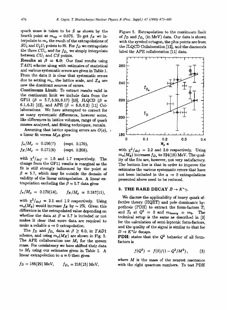
The fD and /Do data at fl _> 6.0, in TAD1 scheme, and using ma(MK) are shown in Fig. 5. The APE collaboration use M1 for the meson mass. For consistency we have shifted their da ta to/1//2 using our estimates given in Table 1. A linear extrapolation to a = 0 then gives

/D = 186(29) MeV, YD, = 218(15) MeV,

Figure 5. Extrapolation to the continuum limit of fD and fDo (in MeV) data. Our data is shown with the symbol octagon, the plus points are from the JLQCD Collaboration [12], and the diamonds label the APE collaboration [11] data.

' ' ' ' I ' r , , I ' ' ' ' I ' ' ' '

260

240

220

~00

, i i ~ I I I I I I I

0.1 0.2 M# a

180 ' l ' ' ' '

0 0.3 0.4

with X2/doI = 2.2 and 2.0 respectively. Using mo(M~) increases fD, to 224(16) MeV. The qual- ity of the fits are, however, not very satisfactory. The bot tom line is that in order to improve the estimates the various systematic errors that have not been included in the a ~ 0 extrapolations presented above need to be reduced.

3. T H E R A R E D E C A Y B ~ K* 7.

We discuss the applicability of heavy quark ef- fective theory (HQET) and pole dominance hy- pothesis (PDH) to extract the form-factors 7'1 and T2 at Q2 = 0 and mh~a,v = rob. The technical setup is the same as described in [3] for the calculation of semi-leptonic form-factors, and the quality of the signal is similar to that for D --+ K'Iv decays. P D H : states that the Q2 behavior of all form- factors is

f(Q2) = f ( 0 ) / ( 1 - Q2/M2), (3)

where M is the mass of the nearest resonance with the right quantum numbers. To test PDH

R. Gupta, T Bhattacharya/Nuclear Physics B (Proc. Suppl.) 47 (1996) 4 73~480 477

Table 1. Our final results at fl = 6.0. All dimensionful numbers are given in M e V with the scale set by Mp. For the systematic errors due to ma, me, q* we also give the sign of the effect. We cannot estimate the uncertainty due to using the quenched approximation, or for entries marked with a ?.

.t,, .fK

fo fD.

fK/f, f, lf. fo./fo

Best Estimate

Statistical & Extrapolation

134 4

159 3

229 7

260 4

1.19 0.02

1.71 0.05

1.135 0.021

Tuning

'¢'ns

- 3

- 5

-0.025

-0.023

Tuning Er~ c

+12

+15

+0.09

+0.006

Tuning q* a (3%) +2 4

+3 5

+4 7

+4 8 I

ZA 10

10

14

20

0 ?

0

Figure 6. Three types of fits to test Q2 behavior of 7"1 using CU3 ~ U1U3 transition. HQET sug- gests a dipole fit if one assumes PDH for T~. The data prefer a pole fit but with the resonance mass smaller than the lattice measured value MD* used to plot the data.

4 ' ' ' ' 1 ' ' ' ' 1 ' ' ' ' 1 ' ' ' ' 1 . . . .

- - Dipole Tt(0 ) = 0.348 / / - - Best Tt(O ) = 0.364 / / 7- --- Pole TI(0 ) = 0.368 / ~

3 / / ~ . . ' " l 7- ~ " •

2

/ /

0.7 0.8 0.9 1 1.1 1.2 (1-Q'Tu~. )

we make two kinds of fits: (i) single parameter "pole" fit where M is the lattice measured value of the resonance mass, (ii) two parameter "best" fit where M and f(0)-are free parameters. Typ- ical examples of these fits are shown in Figs. 6 and 7. Overall, T1 is well described by the "pole" form, whereas T~ has a "flat" Q2 dependence. We take the "best" fit values for our final estimates. H Q E T : To leading order in as and in the mass of the heavy quarks, HQET implies (for heavy to heavy transitions) that the combinations

TlrQ, = T2(O, q2 r o B + m ' i ( " " m B + rn*K 1 - (mB+mK.)~

(4) are independent of the masses of the heavy quarks for fixed velocity transfer. Since T1 (Q2 = 0) = T2(Q 2 = 0) for all mq, this HQET relation and the PDH, F_~t. 3, cannot hold simultaneously. In fact, for heavy quarks (rob + inK.) ~" mpole, therefore, if T~ fits the pole form then T1 must be a 'dipole'. Instead our data, as exemplified in Figs. 6 and 7, prefer a flat T2 and a pole behavior for 7"1. D e p e n d e n c e on quark mass: Figures 8 and 9 show examples of the variation of 7"1 (0) and T2 (0) with quark masses. There is significant de- pendence on the mass of the quark C decays into (which is a kinematic effect), and a slight depen- dence on rns~ct~to,, resulting in the small increase in slope between CUi ---r U1Ui and CUi -r SUi

478 R. Gupta, T. B hattacharya /Nuclear Physics B (Proc. Suppl.) 47 (1996) 473-480

Figure 7. Fits to test Q~ behavior of T2.

3.5 . . . . I . . . . I ' '

3

7~2.5

1 . 5

0 . 8

. . o "

B e s t T = ( 0 ) = 0 . 3 7 7

P o l e T2(0)=0.332

, , , , I , I I I I ,

0 . 9 1 (1-Q=/U=~.)

I I I

1 . 1

Table 2. Estimates of form factors in 3 commonly used renormalization schemes defined in [2]. The data satisfy TI(Q 2 = O) = T2(Q 2 = 0). The last four rows give T(Q 2 = 0) extrapolated to mb using the 4 methods discussed in the text.

TAD1 T1 0.37(2) 2"2 0.39(3) (1) 0.097(2) (2) 0.234(8) (3) 0.084(6) (4) 0.236(12)

TADn TADU0 0.39(2) 0.35(2) 0.40(3) 0.36(2) 0.100(2) 0.091(2) 0.240(8) 0.218(8) 0.086(6) 0.078(5) 0.242(13) 0.220(11)

Figure 8. Extrapolation of 2"1 (Q2 = 0) to m~. The interpolation to rns for TI (B --+ K*7) is done using the points labeled by squares (s = S) and octagons (s = U1), while Tz(B ~ PT) is ob- tained by extrapolating the degenerate qq points (crosses).

: ' ' ' ' I ' ' ' ' I . . . . I . . . .

i 0 4

0 . 3 5

Oe3 . . . . I , , , , I , , , , I , , , ,

0 0.01 0.02 0.03 0.04 m . p

Figure 9. Extrapolation of T2 (Q2 = 0) to m~. The interpolation to me for T2(B ~ K*7) is done using the points labeled by squares (s = S) and octagons (s = 0"1), while T2(B --~ PT) is ob- tained by extrapolating the degenerate qq points (crosse ).

0.45 ' ' ' I . . . . I . . . . I . . . . I

cases, which is consistent with HQET. Ex t r apo l a t i on in mhe=~v: The need to extrap- olate the results obtained at mheavy ~, rnc to mb using HQET, Eq. 4, introduces a very large un- certainty as shown by the four ways of analyzing the data. Methods 1 and 2: we take the value of T2 at zero recoil extrapolated to ms and ~ and scale it to mb using HQET. We can then esti- mate the value at Q2 = 0 assuming pole domi- nance holds for T2 at mb (advocated by A. Soni at this conference), or by using a "flat" behavior as shown by data at mheavv = me. Method 3 (4): Scale T2 (Q2 = 0) (TI) assuming the joint validity of HQET and pole dominance. This implies the

E.-,

0 . 4

0 . 3 5

0 . 3 E L . . . . I i i , I , , , , I , ,

0 0 . 0 1 0 . 0 2 0 . 0 3

m n p

i 1

0 . 0 4

R. Gupta, T. Bhattacharya /Nuclear Physics B (Proc. Suppl.) 47 (1996) 473-480 479

Table 3. Estimates in TAD1 scheme at Q2 = 0. The variations give estimates of systematic errors.

Pole ms(MK) ms(M~) 0.37(2) 0.38(2) 0.37(2) 0.38(2) 0.33(1) 0.34(1) 0.33(1) 0.34(1)

T1 m l m2

T2 mt m2

(i) ml m2

(2) ml m2

(3) mt m2

(4) m~ m2

Best ms(Mg) 0.37(2) 0.37(2) 0.38(3) 0.38(3) 0.096(2) O.lOO(2) 0.230(8) 0.239(9) 0.082(6) o.o95(6)

!o.232(13) 0.242(13)

m.(M÷) 0.37(2) 0.37(2) 0.39(3) 0.39(3) 0.097(2) 0.101(2) 0.234(8) 0.243(9) 0.084(6) 0.096(6) 0.236(12) 0.245(13)

= N "~ ,,.~.-~ 3 / 2 scaling relations T~(Q 2 "/"'he..~u = constant

and T~(Q: = o ) m i / ~ = ~onstant. The results along with their variation with the tadpole sub- traction prescription, type of fit, ms, and the def- inition of heavy-light meson mass (/14"1 or M2) are shown in tables 2 and 3. Resu l t s a t ~ -- 6.0: Methods 1,2 and 3,4 reflect the same contradiction. The value is either 0 .08- 0.1 or 0.23 - 0.25 depending on what we assume for the scaling behavior. With present data we assume that the flat Q2 behavior for 7"2 and pole dominance for 7"1 persists all the way upto the physical value of rob. Then, using the best fit, TAD1 subtraction prescription, ms(M~), and M1 for the meson mass, we get 7"1 = T2 = 0.24(1). Further progress requires clarification of the Q2 behaviour of the form factors and an estimate of the violations of leading order HQET predictions.

4. B - p a r a m e t e r s

We present an update on results for BK, Br, Bs with Wilson fermions evaluated in the NDR scheme with TAD1 subtraction prescrip- tion. Note that both q* and the matching scale between the lattice and continuum theories are taken to be 1/a. Thereafter, the results are run to 2 GeV using the 2-loop relations, however the change is minimal.

To analyze the lattice data (illustrated in Ta-

ble 4) we consider the general form, ignoring chiral logs, of the chiral expansion of the AS = 2 4-fermion matrix elements with Wilson fermions

+ 6~.~p~p: + 63(p~p:) 2 +...(.5)

This follows from Lorentz symmetry as m 2 and Pi "P / a r e the only invariants. BK: The terms proportional to a,fl and 61 are pure lattice artifacts due to mixing of the AS = 2 4-fermion operator with wrong chirality opera- tors. To isolate these terms we fit the data for the lightest 10 mass combinations and for the 5 val- ues of momentum transfer using Eq. 5 as shown in Fig. 10. (Similar values for the six coefficients are obtained from fits to the 6 lightest combinations.) We find that the three 6i are not well determined; only 62 is significantly different from zero. More important, the coefficients 7,62,63 contain arti- facts in addition to the desired physical pieces which we cannot resolve by this method. We simply assume that the l-loop improved opera- tor does a sufficiently good job of removing these residual artifacts. The result then is

BK(NDR, l/a) = 7 + (62 + 63)M~ = 0.65(10).

A second way of extracting BK using Eq. 5 is to combine pairs of points at different momentum transfer:

(El B~: (ql) - E2 BK (q2)) / (E~ - E2) =

7 + 62 m2 + 63re(E1 + F--a).

This procedure directly removes a, fl and 61 but requires a correction to the 63re(E1 + E2) piece, for which we use the value of 63 extracted from the fit. The results of this analysis for the 10 light mass combinations are given in the third column of Table 4. Interpolating to rex, we get Bx(NDR, 1/a) = 0.66(9). BK: The 2-loop running of BK defines the renor- malization group invariant quanti ty/~g [15]

~ = ~.(u) -~/~o (1 + ~o(.)S/4~)BK(.)

where J = (tilT0 - fl07x)/2fl~ = 2.004 for n I = 0. Under running, BK increases as # is de- creased. Thus BK(NDR, 1/a) = 0.66(9) be- comes BK(NDR,2 GeV) = 0.67(9), and BK is

480 R. Gupta, T Bhattacharya/Nuctear Physics B (Proc. Suppl.) 47 (1996) 473-480

Figure 10. Six parameter fit to the BK data.

0.3 ' ' ' ' I ' ' ' ' I ' ' ' ' I . , ' ~ ' '/'~3' '

M a t r i x e l e m e n t o f Lib o p e r a t o r / ~

o

# ----o.33(o.o5) ///3 02 7 = o.4o(o.os) ////÷

~,= o.0o(1.51) ~//// ~,-- 4.88(3.e8) / , ~ / / /

o.1 .~. . / , ,~X' /* o p=(~.oo)

# / ' / / / ~ p--(1 ~ I ) , ¢ , > ' S / , / / ¢ ~, p = ( 1 IO )

A~"/e':~/'/" ~ p=(too) o ~ / + p--(ooo)

~ , - , " S ' ~ l , , , , I . . . . I , , , - , , , , I , , I , , , ,

0 0.05 0.1 0.15 0.2

0.90(14). For comparison, the Staggered value calculated at fl = 6.0 is BK(NDR, 2 GeV) = 0.67 - 0.71 depending on the lattice operators used [13, 14]. An update on staggered results and issues of extrapolation to a --~ 0 have been presented by JLQCD at this conference [14]. B D : The CS, CUi data show no significant variation with momentum transfer as shown in Table 4. The theoretical analysis of artifacts in heavy-light mesons has not yet been com- pleted; indications are that all 6 terms con- tribute. Therefore we simply extrapolate the CUi data to ~ to get BD(NDR, 1/a) = 0.78(1) or BD(NDR, 2 GeV) = 0.79(1). Br and Bs: The chiral expansion is simi- lar to Eq. 5 with all 6 coefficients contain- ing artifacts and physical pieces. Ignoring the artifacts we get Bt(NDR, 1/a) = 0.60(1) and Bs(NDR, 1/a) = 0.81(1) or with 2- loop running B,(NDR, 2 GeV) = 0.59(1) and Bs(NDR, 2 GeV) = 0.81(1). (We find that B8 is very insensitive to changes in # as the running of the matrix element is almost completely canceled by that of its vacuum saturation approximation, while in the case of B~ the two add.) Our es- timate of Bs is smaller than that used in the Standard Model analysis of d /e [15]. Since a smaller Bs means larger 4/e, the calculation of

Table 4. BK, Bt and Bs in NDR renormalization scheme at matching scale #a = 1.

BK ( p = 0 ) ( p = 2 ) subtr.

CC 0.92(1) 0.93(2) c s 0.83(1) 0.85(2) CUt 0.81(1) 0.82(2) cv~ 0.80(1) 0.80(3) CU3 0.79(1) 0.79(4) SS 0.56(0) 0.64(2) su1 0.44(0) 0.57(2) SU2 0.38(1) 0.53(2) su~ 0.34(i) 0.51(3) UIUI 0.24(0) 0.47(2) U~U2 0.11(1) 0.41(3) UtU3 0.00(1) 0.36(3) U2U2 -0.09(1) 0.33(4) U2U3 -0.29(1) 0.26(5) u~v3 -0.60(2) 0.14(7)

B t B8

0.86(1)o.94(1) 0.82(1) 0.94(1) 0.81(1) o.94(1) 0.81(1) 0.94(1) o.80(1) 0.93(1)

0.69(30) 0.72(1) 0.92(i) 0.69(23) 0.70(0) 0.90(1) 0.68(21) 0.68(0) 0.89(1) 0.67(19) 0.67(1) 0.88(1) 0.68(16) 0.66(0) 0.87(1) 0.68(14) 0.64(0) 0.86(1) 0.66(12) 0.63(0) 0.84(1) 0.67(11) 0.62(0) 0.84(1) 0.65(10) 0.60(0) 0.82(1) 0.63(09) 0.58(1) 0.80(1)

Bs is important phenomenologically. Work is in progress to understand and remove various lattice artifacts and make our estimate more reliable.

R E F E R E N C E S

1. T. Bhattacharya, et al., LAUR-95-2354. 2. T. Bhattacharya, R. Gupta, LAUR-95-2355. 3. Bhatt~harya, Gupta, these proceedings. 4. T. Bhattacharya, R. Gupta, Nucl. Phys. B

(PS) 42 (1995) 935. 5. T. Bhattacharya, R. Gupta, in preparation. 6. P. Lepage and P. Mackenzie, Phys. Rev. D48

(1993) 2250. 7. S. Sharpe, Phys. Rev. D41 (1990) 3233, Phys.

Rev. D46 (1992) 3146; J. Labrenz, S. Sharpe, Nucl. Phys. B (PS) 34 (1994) 335.

8. C. Bernard and M. Golterman, Phys. Rev. D46 (1992) 853.

9. It. Gupta, Nucl. Phys. B (PS) 42 (1995) 85. 10. F. Butler, et al., Nucl. Phys. B421 (1994) 217. 11. C. Allton, et al., Nucl. Phys. B (PS) 34 (1994)

456, and private communications. 12. S. Hashimoto, et al., hep-lat/9510033. 13. S. Sharpe, Nucl. Phys. B (PS) 34 (1994) 403. 14. S. Aoki, et al., hep-lat/9510012. 15. M. Ciuchini, et al., Z. Phys. C68 (1995) 239.