STAR-CCM+ User Guide Steady Flow: Lid-Driven Cavity Flow 2 Version 7.03.027 Steady Flow: Lid-Driven Cavity Flow This tutorial demonstrates the performance of STAR-CCM+ in solving a traditional square lid-driven cavity flow. The problem geometry consists of a two-dimensional 1 m 2 cavity, covered by an impermeable wall that moves in the x-direction with constant velocity of 1 m/s. A stretched quadrilateral mesh with 6400 cells is used. Material properties: Boundary conditions: Density (kg/m 3 ) 1.0 Dynamic viscosity (PaS) 0.0002 Top wall U = 1.0 (m/s), V=0.0 Bottom wall U = V = 0.0
Transcript
STAR-CCM+ User Guide Steady Flow: Lid-Driven Cavity Flow 2
Steady Flow: Lid-Driven Cavity Flow
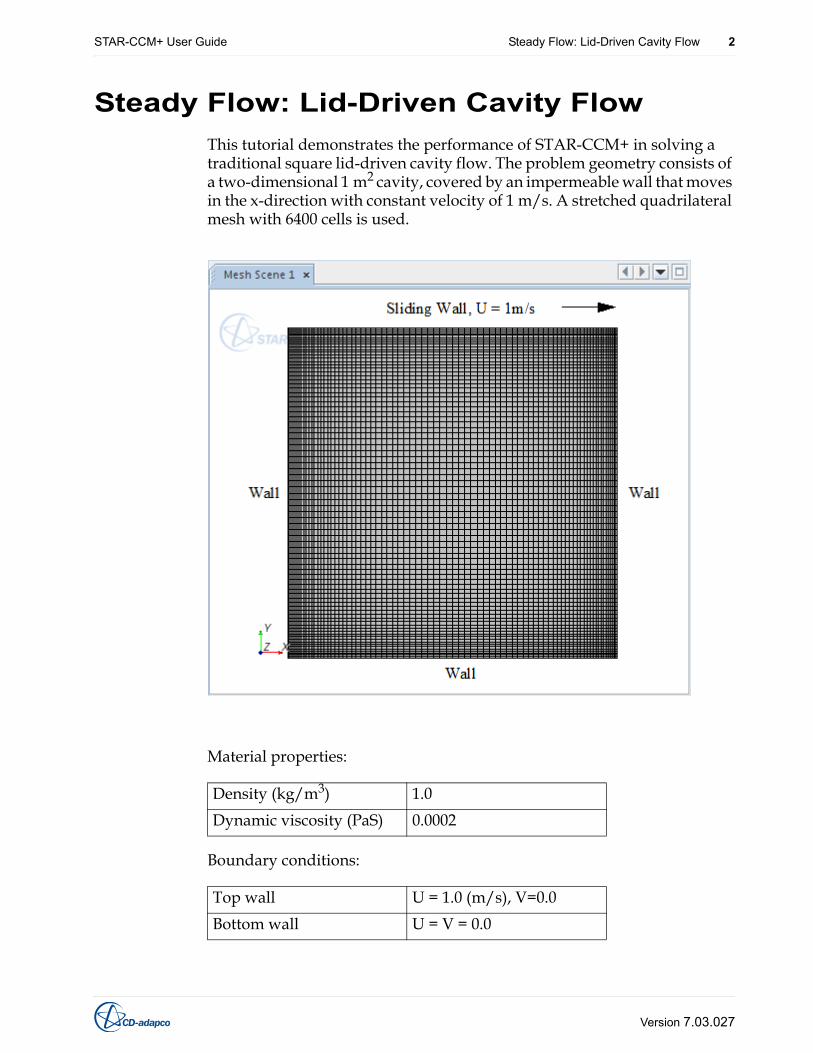
This tutorial demonstrates the performance of STAR-CCM+ in solving a traditional square lid-driven cavity flow. The problem geometry consists of a two-dimensional 1 m2 cavity, covered by an impermeable wall that moves in the x-direction with constant velocity of 1 m/s. A stretched quadrilateral mesh with 6400 cells is used.
Material properties:
Boundary conditions:
Density (kg/m3) 1.0
Dynamic viscosity (PaS) 0.0002
Top wall U = 1.0 (m/s), V=0.0
Bottom wall U = V = 0.0
Version 7.03.027
STAR-CCM+ User Guide Steady Flow: Lid-Driven Cavity Flow 3
Initial conditions:
The Reynolds number based on the width of the cavity, top wall velocity, fluid density and fluid dynamic viscosity is 5000. The calculation is performed using the Segregated Flow model. Both the U- and V-velocity profiles along lines passing through the center of the cavity are compared with data from the literature [1].
Importing the Mesh and Naming the Simulation
Start up STAR-CCM+ in a manner that is appropriate to your working environment and select the New Simulation option from the menu bar. STAR-CCM+ will create a window for the new simulation in the Explorer pane and give it the default name Star 1.
A quadrilateral-cell mesh has been prepared for this analysis and is stored in a .ccm format file. Import it into the simulation:
• Select File > Import > Import Volume Mesh... from the menu bar.
• In the Open dialog, navigate to the doc/tutorials/simpleFlow subdirectory of your STAR-CCM+ installation directory and select the file cavityQuad.ccm.
• Click the Open button to start the import.
STAR-CCM+ will provide feedback on the import process in the Output window. A mesh region named cell-2 is created under the Regions node to represent the solution domain.
• Save the new simulation to disk as cavityQuad.sim.
Visualizing the Imported Mesh
We will view the imported mesh, and access various parts contained in the region.
• Right-click the Scenes node and then select New Scene > Mesh. The mesh will appear in a new scene in the Graphics window.
• The edges of the square are boundaries. Click on one of them. The
Left wall U = V = 0.0
Right wall U = V = 0.0
U, V velocity components (m/s) 0.0
Operating pressure (Pa) 0.0
Version 7.03.027
STAR-CCM+ User Guide Steady Flow: Lid-Driven Cavity Flow 4
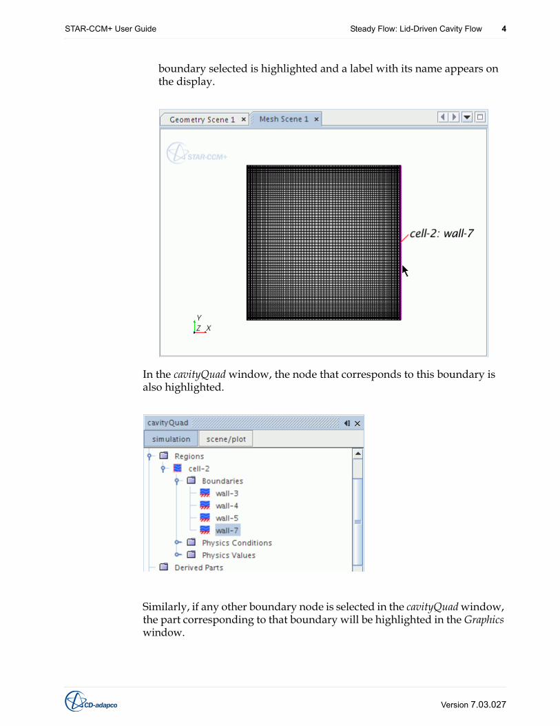
boundary selected is highlighted and a label with its name appears on the display.
In the cavityQuad window, the node that corresponds to this boundary is also highlighted.
Similarly, if any other boundary node is selected in the cavityQuad window, the part corresponding to that boundary will be highlighted in the Graphics window.
Version 7.03.027
STAR-CCM+ User Guide Steady Flow: Lid-Driven Cavity Flow 5
Setting up the Models
The default continuum (Physics 1) will be edited so that the appropriate physical models for the simulation are selected.
To select physical models for this continuum:
• Right-click the Continua > Physics 1 > Models node and choose the item Select models...
The Physics 1 Model Selection dialog will guide us through the model selection process by showing only options that are appropriate to the choices made so far.
In the Physics 1 Model Selection dialog:
• Ensure that the Auto-select recommended models checkbox is ticked.
• Make sure that Two Dimensional and Gradients are selected.
• Select Liquid in the Material group box.
• Select Segregated Flow in the Flow group box.
• Select Constant Density in the Equation of State group box.
• Select Steady in the Time group box.
• Select Laminar in the Viscous Regime group box.
• Click Close.
The color of the Physics 1 node has turned from gray to blue to indicate that models have been activated.
• Save the simulation .
Version 7.03.027
STAR-CCM+ User Guide Steady Flow: Lid-Driven Cavity Flow 6
Setting Fluid Properties
The density and dynamic viscosity fluid properties must be set.
• Select the Continua > Physics 1 > Models > Liquid > H2O > Material Properties > Density > Constant node.
• In the Properties window, set the Value to 1.0 kg/m^3.
• Within the same H2O node, select the Constant node in the Dynamic Viscosity node. Set the Value to 2.0E-4 Pa-s.
Setting Boundary Conditions and Values
This problem requires only two boundary conditions: moving and stationary. In STAR-CCM+ it is possible to combine two or more boundaries into one.
• In the cavityQuad window, open the Regions > cell-2 > Boundaries node.
• Use the <Ctrl><Click> approach to select the boundary nodes wall-3,
Version 7.03.027
STAR-CCM+ User Guide Steady Flow: Lid-Driven Cavity Flow 7
wall-4 and wall-7.
• Right-click and select Combine. This will create a single boundary, wall-3, that consists of all sides of the square except the top.
• Right-click on the wall-3 node and rename it Stationary Wall.
• Rename the wall-5 boundary node Moving Wall.
For the moving wall boundary, the velocity of 1 m/s in the x-direction needs to be set.
• Open the Moving Wall > Physics Conditions node and select the Tangential Velocity Specification node.
• In the Properties window, select Vector from the drop-down list of the Method property.
Version 7.03.027
STAR-CCM+ User Guide Steady Flow: Lid-Driven Cavity Flow 8
• Now open the Physics Values node that was added to the object tree.
• Open the Velocity node and select the Constant node.
• Enter 1,0,0 in the Value property.
• Save the simulation .
Visualizing the Solution
Post-processing scenes can be updated every iteration (or time-step) in STAR-CCM+. This allows for dynamic monitoring of various quantities, such as the velocity that we want to visualize in this tutorial. A vector scene will therefore be created prior to running.
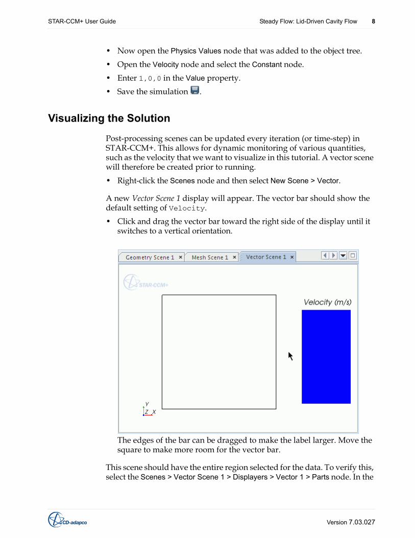
• Right-click the Scenes node and then select New Scene > Vector.
A new Vector Scene 1 display will appear. The vector bar should show the default setting of Velocity.
• Click and drag the vector bar toward the right side of the display until it switches to a vertical orientation.
The edges of the bar can be dragged to make the label larger. Move the square to make more room for the vector bar.
This scene should have the entire region selected for the data. To verify this, select the Scenes > Vector Scene 1 > Displayers > Vector 1 > Parts node. In the
Version 7.03.027
STAR-CCM+ User Guide Steady Flow: Lid-Driven Cavity Flow 9
Properties window, the Parts property should show cell-2, the name of the region.
Setting up Lines for Plotting
Data will be plotted for both the U- and V-velocity profiles along line probes passing through the center of the cavity. To create these lines:
• Make sure at least one scene display is active in the Graphics window.
• Right-click on the Derived Parts node and select New Part > Probe > Line...
Version 7.03.027
STAR-CCM+ User Guide Steady Flow: Lid-Driven Cavity Flow 10
The Create Line Probe dialog will appear in the Explorer pane to specify the desired line. The following settings will be for the U line.
• In the Input Parts group box, cell-2 should be the only part.
• Change Point 1 to [0.5, 0, 0] m.
• Change Point 2 to [0.5, 1, 0] m.
• Specify the Resolution at 50.
• Under Display, select the No Displayer radio button.
• Click Create, then click Close.
Version 7.03.027
STAR-CCM+ User Guide Steady Flow: Lid-Driven Cavity Flow 11
A new derived part named line-probe will be created in the Derived Parts manager node.
• Rename this node Simulation (U).
Next, the V line probe needs to be created. This can be done simply by making a copy of the existing derived part and modifying it.
• Right-click on the Simulation (U) node and select Copy.
• Right-click on the Derived Parts node and select Paste.
• Rename the new node Simulation (V).
• In the Properties window, enter 0, 0.5, 0 for the Point 1 property.
• Enter 1, 0.5, 0 for the Point 2 property.
• Save the simulation .
Plotting Simulation Data
This part of the tutorial produces the plots of the U- and V-velocity profiles. In a subsequent step, experimental data will be imported from files and plotted alongside the numerical data. The development of the solution can be observed throughout the run by viewing these plots.
To create the U-velocity plot:
• Right-click on the Plots node and select New Plot > X-Y. A new node named XY Plot 1 will appear.
• Rename the XY Plot 1 node U-Velocity Profile.
• With this node still selected, in the Properties window, click on the right-hand side of the Parts property. Select Derived Parts > Simulation (U) in the Parts dialog and click OK.
Version 7.03.027
STAR-CCM+ User Guide Steady Flow: Lid-Driven Cavity Flow 12
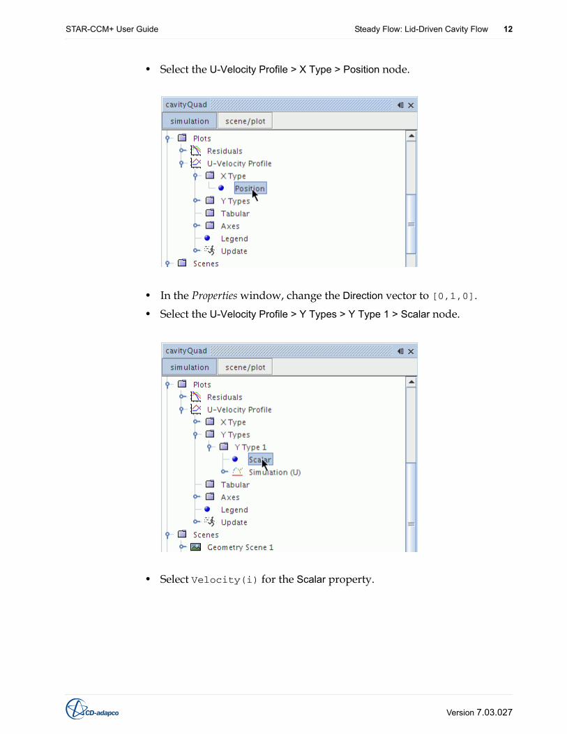
• Select the U-Velocity Profile > X Type > Position node.
• In the Properties window, change the Direction vector to [0,1,0].
• Select the U-Velocity Profile > Y Types > Y Type 1 > Scalar node.
• Select Velocity(i) for the Scalar property.
Version 7.03.027
STAR-CCM+ User Guide Steady Flow: Lid-Driven Cavity Flow 13
• In the same Y Type 1 node, select the Simulation (U) > Line Style node.
• In the Properties window, change the Style property to Solid.
• Select the Symbol Style node.
• Change the Shape property to None.
• Select the U-Velocity Profile > Axes > Y Axis > Labels node.
• Change the Minimum and Maximum properties to -0.6 and 1.0, respectively.
• Change the Label Spacing expert property to 0.2.
To create the V-velocity plot:
• Right-click on the Plots node and again select New Plot > X-Y. A new node named XY Plot 1 will appear.
• Rename this XY Plot 1 node V-Velocity Profile.
• With this node still selected, in the Properties window, click on the right-hand side of the Parts property. Select Derived Parts > Simulation (V) in the Parts dialog and click OK.
• Select the V-Velocity Profile > Y Types > Y Type 1 > Scalar node.
• Select Velocity(j) for the Scalar property.
• In the same Y Type 1 node, select the Simulation (V) > Line Style node.
• In the Properties window, change the Style property to Solid.
Version 7.03.027
STAR-CCM+ User Guide Steady Flow: Lid-Driven Cavity Flow 14
• Select the Symbol Style node.
• Change the Shape property to None.
• Select the V-Velocity Profile > Axes > Y Axis > Labels node.
• Change the Minimum and Maximum properties to -0.7 and 0.5, respectively.
• Change the Label Spacing expert property to 0.2.
• Save the simulation .
Plotting Reference Data
To compare the experimental velocity data with the velocity plots, it is necessary to import the data in supplied files into STAR-CCM+ tables:
• Open the Tools node.
• Right-click on the Tables node and select New Table > File....
• In the Open dialog navigate to the doc/tutorials/simpleFlow subdirectory of your STAR-CCM+ installation directory, set the File Type drop-down list to (*.xy), and select the file UVelocity.xy.
• Click Open.
The data in that file is now stored in a table named UVelocity. To display it on the U-velocity plot:
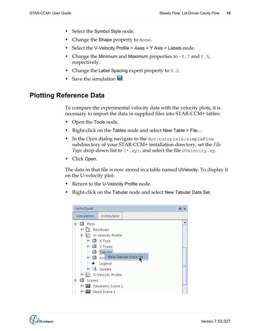
• Return to the U-Velocity Profile node.
• Right-click on the Tabular node and select New Tabular Data Set.
Version 7.03.027
STAR-CCM+ User Guide Steady Flow: Lid-Driven Cavity Flow 15
A new node named tabular will appear.
• In the Properties window, select UVelocity for the Table property.
• Rename the node Reference Data (U).
• Select column 0 for the X column and column 1 for the Y column.
• Select the Reference Data (U) > Line Style node.
• In the Properties window, make sure that the Style property is set to None.
• Select the Symbol Style node.
• Change the Size property to 6.
• Change the Color property to blue.
• Change the Shape property to Triangle.
The supplied experimental data will now appear in the U-velocity plot. Numerical data will be shown once the simulation run has started.
Use the same techniques for the V-velocity plot:
• Right-click on the Tables node and select New Table > File....
• In the Open dialog, select the file VVelocity.xy and click Open.
• In the V-Velocity Profile > Tabular node, create a new tabular data set and select VVelocity for the Table property.
• Rename the node Reference Data (V).
• Select column 0 for the X column and column 1 for the Y column.
• Select the Reference Data (V) > Line Style node.
• In the Properties window, make sure that the Style property is set to None.
• Select the Symbol Style node.
• Change the Size property to 6.
• Change the Color property to blue.
• Change the Shape property to Triangle.
Now both plots will show experimental data alongside the numerical data.
• Save the simulation .
Preparing Solver Parameters and Stopping Criteria
Before running the analysis, we will take a look at the velocity solver, as well as the maximum number of iterations to be performed.
Version 7.03.027
STAR-CCM+ User Guide Steady Flow: Lid-Driven Cavity Flow 16
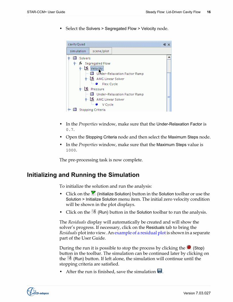
• Select the Solvers > Segregated Flow > Velocity node.
• In the Properties window, make sure that the Under-Relaxation Factor is 0.7.
• Open the Stopping Criteria node and then select the Maximum Steps node.
• In the Properties window, make sure that the Maximum Steps value is 1000.
The pre-processing task is now complete.
Initializing and Running the Simulation
To initialize the solution and run the analysis:
• Click on the (Initialize Solution) button in the Solution toolbar or use the Solution > Initialize Solution menu item. The initial zero velocity condition will be shown in the plot displays.
• Click on the (Run) button in the Solution toolbar to run the analysis.
The Residuals display will automatically be created and will show the solver’s progress. If necessary, click on the Residuals tab to bring the Residuals plot into view. An example of a residual plot is shown in a separate part of the User Guide.
During the run it is possible to stop the process by clicking the (Stop) button in the toolbar. The simulation can be continued later by clicking on the (Run) button. If left alone, the simulation will continue until the stopping criteria are satisfied.
• After the run is finished, save the simulation .
Version 7.03.027
STAR-CCM+ User Guide Steady Flow: Lid-Driven Cavity Flow 17
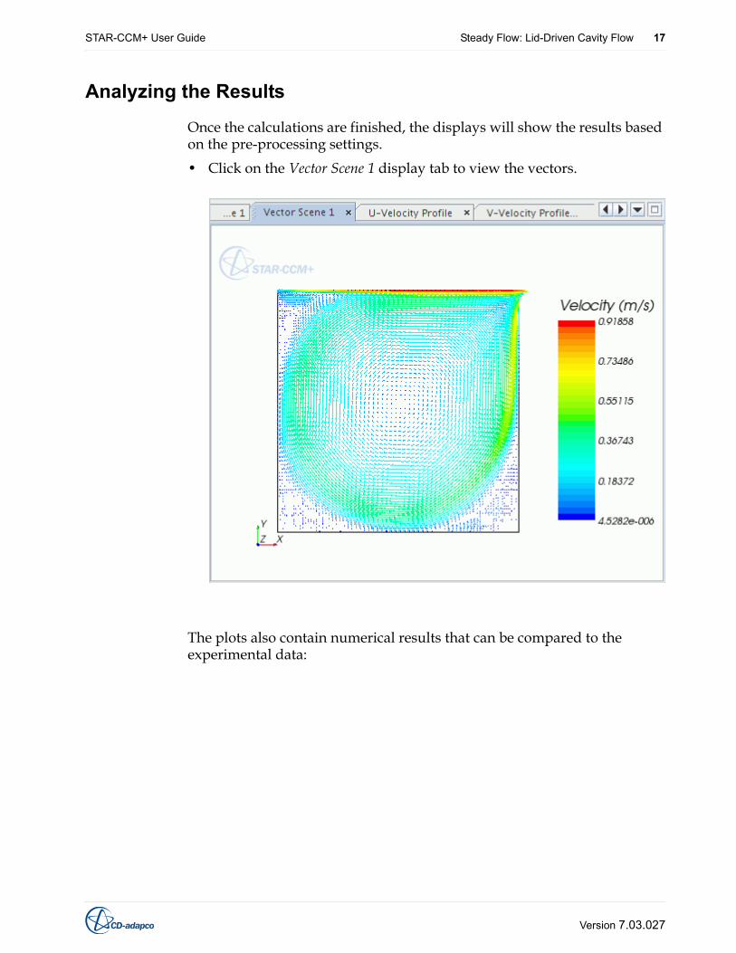
Analyzing the Results
Once the calculations are finished, the displays will show the results based on the pre-processing settings.
• Click on the Vector Scene 1 display tab to view the vectors.
The plots also contain numerical results that can be compared to the experimental data:
Version 7.03.027
STAR-CCM+ User Guide Steady Flow: Lid-Driven Cavity Flow 18
• U-velocity
Version 7.03.027
STAR-CCM+ User Guide Steady Flow: Lid-Driven Cavity Flow 19
• V-velocity
Summary
This tutorial demonstrated the following STAR-CCM+ features:
• Defining physical models.
• Defining material properties required for the selected models.
• Defining boundary conditions.
• Reviewing solver parameters and stopping criteria.
• Monitoring the solution progress.
• Running the solver until the residuals are satisfactory.
• Analyzing results using STAR-CCM+’s visualization and XY-plot facilities.
Bibliography[1] Ghia, U., Ghia, K.N., and Shir, C.T. 1982. “High-Re solution for
incompressible flow using the Navier-Stokes equations and a multigrid method”, J. Comp. Phys., 48, p. 387.