Steering and Visualization of Electro-MagneticSimulations Using the Globus Implementation of aComputational Grid

Erik Engquist

NADA, Royal Institute of Technology

Abstract A framework for computational steering of a finite difference code for electro-magnetic simulation has been developed and implemented. In computational steering weneed to develop software which allows the user to enter an interactive visualization or VRenvironment and from there control the computation.

A proof of concept implementation has been carried out using an existing code for 3Dfinite difference time domain approximation of Maxwell’s equations. Large parts of the com-putational steering software are general but details in the choice of control variables andvisualization is specialized to the electromagnetics code.

To handle the large computational requirements of both simulation and visualization thesystem can be distributed across multiple machines. This is possible through the use of theGlobus toolkit for communication, data handling, and resource coallocation. It program alsomakes use of VTK for data filtering and the generation of visualization elements, and IRISPerformer with pfCAVELib for 3D interactive rendering on CAVE compatible devices.

Two testcases are presented. In one example with a smaller number of computationalcells, full computational steering with recomputation is possible. In another with a largenumber of computational cells the solution is precomputed and only the visualization is in-teractive. The scalability of the computational code is tested for different computers in orderto determine the size of the problem which can be handled with full computational steeringon the available local hardware.

1 Introduction

The objective of this project is to produce a framework for a distributed compu-tational steering code. The framework will be implemented with a computationalcode used for large-scale Finite Difference Time Domain (FDTD) electro-magneticcalculations. In electro-magnetic simulations the electric and magnetic fields andsurface currents are computed. Typical applications are in electro-magnetic com-patibility, radar cross section research, and antenna design.

To enable visualization and interaction in a 3D immersive environment, the codemade use of the Visualization Toolkit (VTK) [8] in combination with IRIS Per-former [2] and pfCAVELib [6]. The graphics facilities on which this project hasbeen run include an ImmersaDesk and the VR-Cube at PDC. In one application,the program was used for the interactive visualization of the results of a very largeFDTD computation. The geometry contained two million polygons and the domainof computation consisted of over a billion cells. This was made possible through theuse of data decomposition, parallelization, and variable levels of detail.

A user interface was also created as part of the project. Interaction is carried outthrough the use of a tracked wand and floating menu buttons. The user may chooseto display different features of the computed solution. Examples of such featuresinclude surface currents, electric or magnetic fields in cutting planes, and electric ormagnetic field strength iso surfaces. Regarding interaction with the computationalprocess, the user can stop and start the computation as well as adjust all the simula-tion parameters.

The Nexus [4] communication library from the Globus toolkit is used to con-nect the flow of control information from the visualization process to the compu-tation process and the flow of computed data in return. Nexus is a multi-threadedcommunication library which is especially well suited for a heterogeneous comput-ing environment, as well as the event driven nature of the communication. Via thiscomputational grid implementation, the application has made use of computationalresources ranging from a Linux cluster to an IBM SP.

The final product consists approximately 4,000 lines of FORTRAN90, C, andC++ code. There are also additional shell script routines used in organizing andconfiguring the package. The computational code has been edited to communicatewith the visualization code as well as be interactively controlled by the user. Datatransfer and translation routines have been written for the exchange of informa-tion between separate processes. Synchronization structures and routines have beencreated to allow multi-threaded communication. A visualization code was writtenwhich handles both geometric and volume data with multiple methods of presenta-tion. The displayed information can be manipulated in an immersive environmentusing a wand and menu interface.

2 Problem

For the implementation of the steering and visualization package we chose an exist-ing computational code. Since the code is a part of a much larger project, we neededto minimize the changes required to the preexisting code.

2.1 The Numerical Scheme

The Yee scheme [10] is used, which is a centered finite difference approximation ofMaxwell’s equations,

∂E

∂t=

1ε∇×H − J (1)

∂H

∂t= − 1

µ∇× E (2)

∇ · E = 0 (3)

∇ ·H = 0 . (4)

The three dimensional electric,E(x, t), and magnetic,H(x, t), fields are defined asfunctions of space,(x ∈ Ω), and time,

(IR4 → IR6

). The currentJ(x, t) is regarded

as a forcing term and the material parameters, permittivity,ε(x), and permeability,µ(x), could be space dependent. The electric and magnetic fields are divergencefree.

The most common numerical approximation of (1) and (2) is the Yee scheme,which is based on centered differences in space and time. This means it is a leap-frog scheme applied to Maxwell’s equations on a staggered grid. The Yee schemehas the advantage that very few operations are required per grid point. TheE evo-lution depends onH and vice versa, while the matricesAx, Ay, andAz are sparse.Additionally, the discrete forms of (3) and (4) are preserved by the scheme. A typicaldifference step for the x-component ofE looks like,

En+1x,i,j,k =

Enx,i,j,k + ∆tεi,j,k

Hn+ 1

2z,i,j+ 1

2 ,k−H

n+ 12

z,i,j− 12 ,k

∆y −Hn+ 1

2y,i,j,k+ 1

2−H

n+ 12

y,i,j,k− 12

∆z

. (5)

Absorbing boundary conditions of different types are possible at open boundarieswhich limit the computational domain [9].

2.2 The FDTD Code

This code was a part of the Large Scale FDTD project, GEMS [1], within theParallel and Scientific Computing Institute (PSCI). The programming language isFORTRAN90 with MPI message passing. Domain decomposition is used as a ba-sis for parallelization. The input to the code consists on an initialization file whichdescribes simulation parameters and defines the names of files which describe ge-ometry, sources, and output. These output files contain the electro-magnetic fieldsand surface currents. Modifications to the code have been quite limited to rewritingthe initialization and output routines. A goal of the project was to require minimalchanges to the computational code in order to simplify its integration into existingprojects.

The solver originally consisted of almost 5,000 lines of code, the changes amountedto the removal of a initialization file read in function and two result write out com-mands. These were replaced by corresponding data I/O routines in the communica-tion code. Inside the main computational loop we also added a call to a state updatefunction in the communication code.

The number of FLOPs required each time-step of the computational code isapproximatelyNx × Ny × Nz × 36 for each field, whereNx, Ny, andNz arethe size of the computational domain. Unfortunately, (5) shows that there are sixunknowns for each component update. On scalar architecture machines, this willmean a high memory access to computation ratio which result in the inherent mem-ory fetch penalties.

The performance of this code on the Linux cluster was around 80-90 MFLOP/sper node. On the four way 333MHz PowerPC 604e SMP nodes on the SP, perfor-mance rose to 220-240 MFLOP/s per node, while the Power2 nodes performed at

180-190 MFLOP/s. This type of information is useful for gauging the feasibility ofsteering a particular computation. One can look at the performance requirements ofa particular case and then demand the necessary hardware. More likely, one can seethe limits a given hardware sets and scale the size of the computation appropriately.

The basic performance requirements show the necessity of distributed comput-ing for this case. Since the visualization machine is burdened by transforming thefield data and generating geometric elements, it cannot simultaneously support largescale numerical computations.

3 Resources

At the Center for Parallel Computers at KTH (PDC) there exists a broad range ofhardware resources. We made use of hardware systems for visualization, computa-tion, and communication.

3.1 Visualization Resources

Of special interest to this project were the visualization facilities at PDC, includ-ing the VR-Cube, a six walled immersive environment. The Cube is driven by a12 processor SGI Onyx2 with three InfiniteReality2 pipes. As a development plat-form there exists an ImmersaDesk which is connected to a dual processor SGI Oc-tane with EMXI graphics. These two facilities both support CAVELib and IRISPerformer making development for both completely identical. A tracking systemdetermines the location of the viewer and adjusts the 3D images accordingly.

The VR-Cube, is a projection based immersive environment with six walls. Theinterior of the Cube measures3 × 3 × 2.5 meters. The rear wall is hinged and theCube is raised 2.5 meters above the floor to allow rear projection on all six sides.This removes any shadows due to users and allows for a completely immersive en-vironment. The depth effect is achieved through the use of liquid crystal shutteredglasses. Images for the left and right eye are alternated as an IR transmitter synchro-nizes the glasses. The wall resolutions are1152×960 while the floor and ceiling are1152× 1152. Each graphics pipe drives two screens at a frequency of 96Hz, whichin turn means the user experiences stereo images at a frequency of 48Hz per eye.

3.2 Computation Resources

The computational resources are even more varied. For initial development the com-putation was carried out on the visualization machine itself. Once distributed com-putation was implemented the development continued on a Linux cluster. The clus-ter consists of eight dual Intel Pentium II nodes. The processors run at 350MHz andthe nodes have 256MB of memory. Communication between the nodes consists offast Ethernet NICs connected to a central switch. This machine was lightly loadedand well suited for development purposes. The heavier computational runs werecarried out on an IBM SP. Some SP nodes have 160MHz Power2 processors and

others have 4-way PowerPC processors operating at 333MHz. The Power2 nodeshave 256MB memory while the SMP nodes have 512MB. The SP machine beingone of the main computational resources at PDC is heavily loaded and therefor notas well suited for development work.

4 Implementation

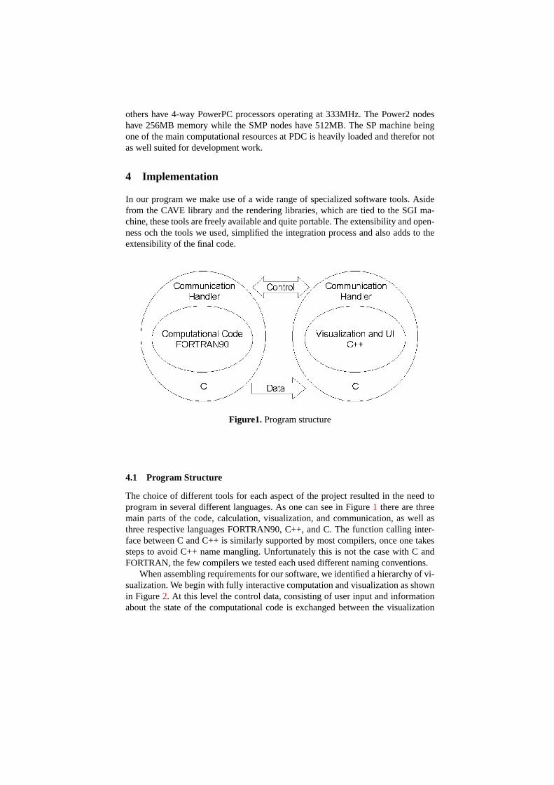
In our program we make use of a wide range of specialized software tools. Asidefrom the CAVE library and the rendering libraries, which are tied to the SGI ma-chine, these tools are freely available and quite portable. The extensibility and open-ness och the tools we used, simplified the integration process and also adds to theextensibility of the final code.

Figure1. Program structure

4.1 Program Structure

The choice of different tools for each aspect of the project resulted in the need toprogram in several different languages. As one can see in Figure1 there are threemain parts of the code, calculation, visualization, and communication, as well asthree respective languages FORTRAN90, C++, and C. The function calling inter-face between C and C++ is similarly supported by most compilers, once one takessteps to avoid C++ name mangling. Unfortunately this is not the case with C andFORTRAN, the few compilers we tested each used different naming conventions.

When assembling requirements for our software, we identified a hierarchy of vi-sualization. We begin with fully interactive computation and visualization as shownin Figure2. At this level the control data, consisting of user input and informationabout the state of the computational code is exchanged between the visualization

and computation hardware. This data is asynchronous and low volume. The com-puted data consists of much more information and moves only from the calculatingmachine to the visualization machine.

Figure2. Computational steering

The final level of this visualization hierarchy can be seen in Figure3. This issimply post processing data visualization. After a computational run has been com-pleted, the results are saved to disk and visualization work can begin on the data set.In this case the user does not have interactive control of the computation, but thecalculations may be so demanding that interactivity is not a reasonable possibility.

Figure3. Interactive visualization

4.2 Visualization

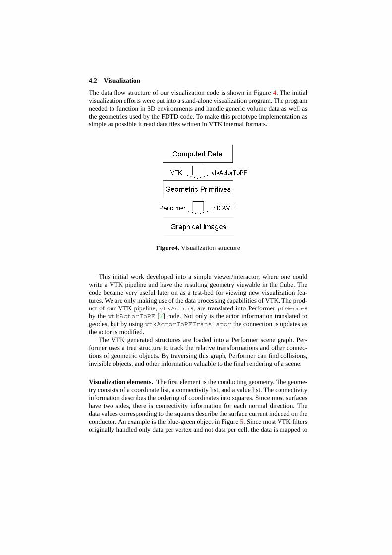
The data flow structure of our visualization code is shown in Figure4. The initialvisualization efforts were put into a stand-alone visualization program. The programneeded to function in 3D environments and handle generic volume data as well asthe geometries used by the FDTD code. To make this prototype implementation assimple as possible it read data files written in VTK internal formats.

Figure4. Visualization structure

This initial work developed into a simple viewer/interactor, where one couldwrite a VTK pipeline and have the resulting geometry viewable in the Cube. Thecode became very useful later on as a test-bed for viewing new visualization fea-tures. We are only making use of the data processing capabilities of VTK. The prod-uct of our VTK pipeline,vtkActor s, are translated into PerformerpfGeode sby thevtkActorToPF [7] code. Not only is the actor information translated togeodes, but by usingvtkActorToPFTranslator the connection is updates asthe actor is modified.

The VTK generated structures are loaded into a Performer scene graph. Per-former uses a tree structure to track the relative transformations and other connec-tions of geometric objects. By traversing this graph, Performer can find collisions,invisible objects, and other information valuable to the final rendering of a scene.

Visualization elements.The first element is the conducting geometry. The geome-try consists of a coordinate list, a connectivity list, and a value list. The connectivityinformation describes the ordering of coordinates into squares. Since most surfaceshave two sides, there is connectivity information for each normal direction. Thedata values corresponding to the squares describe the surface current induced on theconductor. An example is the blue-green object in Figure5. Since most VTK filtersoriginally handled only data per vertex and not data per cell, the data is mapped to

the vertices of the square. For performance and storage reasons these squares arethen triangulated and connected into triangle strip structures. To make the currentinformation more clear, a logarithmic color scale is used.

Figure5. Iso value surface of electric field strength(red) and surface currents on aconductor

The volume data consists ofEx, Ey, Ez,Hx,Hy, andHz values at each point.There are almost endless ways one can display this data, here a user can take advan-tage of VTK’s versatility and add whatever objects they would want. Currently wehave implemented iso value surfaces, cutting planes, and a vector probe.

The iso value surface is implemented using thevtkContourFilter class. Auser can select whether to view the strength of a particular component of the electricor magnetic fields, or the total field strength. Through the user interface described inSection4.3 the user can set at which value the iso surface should be displayed. Theiso surface is represented as triangle strips just like the PEC elements, the surface isalso made transparent so that it does not hide any other structures which are beingdisplayed, the transparent red object in Figure5 is an iso value surface.

Cutting planes can be used to display individual field component strengths aswell as total field strength. In this case, two different methods have been used. Forsmaller data sets there is a general plant which the user can move with the wand.

This implementation makes use ofvtkClipVolume andvtkPlane . Unfortu-nately the implicit function clipping in VTK is not a particularly fast operation,therefor we also created a cutting plane for the large data set usingvtkExtractVOI .This plane is restricted to remain orthogonal to thex, y, or z axis. Such a cuttingplane is visible in Figure6.

Figure6. Cutting plane inside a large model

Finally, the vector probe is used to inspect data at a given point. At the end ofthe wand, a vector will point in the direction of the electric and/or magnetic field,see Figure7. This vector is scaled by the magnitude of the vector. There is also andoption for the separate component vectors to be shown. The numerical informationat a point, as well as the global maximum and minimum values used in scalingthe vector come from the VTK data pipeline. The actual vector arrow is Performerobject. While this may not be the cleanest implementation, it was done mainly forperformance reasons.

Presentation of geometries.VTK data consists of several parts. One part consistsof the scalar values, in our case the results of the computations. Another element arethe coordinate points of the data. In the case of the free fields this is very structureddata while the conducting geometry is not as regular. Finally the points are organizedin terms of connectivity describing cells. Cells are the basic geometric elements such

as points, lines, triangles, etc. Currently VTK contains twelve different cell types,ranging from 1D to 3D cells. The data consisting of points, cells, and values arewhat is manipulated by VTK to be rendered on screen.

Figure7. Vector probe of electric and magnetic fields

Presentation of volume data. Computational codes such as the CEM code usedfor this project produce data for the whole domain of computation. How to viewthis data in an efficient and understandable manner is an important question. Whilevolume rendering can be defined generally as the rendering of volumetric data, itis more common to use the term in reference to specific volumetric display meth-ods. These methods are the ones which directly use 3D primitives such as tetrahedraand voxels. VTK containsvtkVolumeRayCast classes for volume rendering im-plementing ray casting techniques. There is also some progress in using hardwareobject ordering techniques, and one can also look at SGI’s Volumizer library. Unfor-tunately this type of visualization is very demanding and not well suited for largervolumes, especially in interactive applications. There are many methods one can useto produce the effect of true volume rendering or present volume data in a form lesstaxing on the machine.

Less demanding rendering methods involve the use of 2D objects to presentvolume data. Several transparent cutting planes placed in parallel for example, canbe combined to present information about the volume at several different levels.Iso value surfaces calculated pointwise can present information similarly to such asurface generated through a ray casting method. Due to the need for interactivity inthe application we decided to use these simpler methods to display data.

Large data sets. As one can see in Section2.2, the problem size is limited by theinteractivity of the computation. However, one could imagine the case where thecomputation produced more data than can be interactively displayed. A test of thiscase presented itself at a meeting of the General ElectroMagnetic Solvers (GEMS)project in June ’99. Here the data from a large run was to be shown in the VR-Cube. The geometry consisted 2 million polygons, and the volume of computationconsisted of1260× 1260× 635 cells.

To approximate the limits of the available hardware we made some simple cal-culations. SGI specifications state a peak polygon rate for an InfiniteReality2 pipearound 13M polygons/s, this is split over two screens, leaving 6.5M. polygons/s ifthe walls are equally loaded. In stereo, one needs a separate image per eye, thisleaves 3.25M. polygons/s. For the appearance of motion one needs≈ 20 frames persecond which brings us to 163K. polygons/frame. Of course all things are seldomoptimal and a more reasonable count is around 100K. polygons. Again, the hard-ware performance sets a limit for the complexity of the problem to be displayed.In this case it is not the computational load, but the amount of conducting objects,surfaces, menus, which must react to the user in an immersive environment.

The raw geometric data was not suitable to be displayed in the Cube. To min-imize the changes in a relatively working code, we felt the best approach was tocreate a data set better suited for interactivity. Initially, all information not visiblefrom the inside of the plane was clipped. This was done rather simply by includ-ing only the geometry which fit inside a cylinder with the dimensions of the cabin.In this way, the wings and tail section were removed from the data set. The nextstep was removing information in the shell of the plane which faced outwards. Thestructure of the data produced by the CEM code is such that two identical cells areproduced for each wall. These cells differ in scalar values as well as normal direc-tions, thus producing an inside and outside wall. Taking the cross productn × c,wheren is the normal of a cell andc faces from the centroid of the plane to thecell, gives us−1 for outwards facing cells. At this point the data consisted of 300thousand polynomials.

A useful technique when dealing with large data sets is to use multiple levels ofdetail (LOD). Objects which are closer to the viewer should be fully resolved, whilefar away details need not be shown as clearly. Optimally one would want this lossof detail to be continuous and relatively unnoticable to the viewer. Both Performerand VTK have facilities for the handling of LODs. ThevtkLODActor in VTKis a simple implementation where an object is replaced by progressively simplerobjects depending on the amount of CPU time allocated to the renderer. The defaultimplementation starts with the full object then steps to a point cloud and finally to

an outline box. Performer on the other hand has very advanced LOD capabilitiessuch aspfASD or active surface definition.

The most straightforward LOD method is similar to the one which exists inVTK. Here apfLOD is created with different levels for each object. The user canthen choose to switch between levels depending on the machine load or distancefrom the observer. To minimize the “blinking” effect of one object being replacedby another, the user can define a blending zone. In the blend zone, both objectsare displayed with varying opacity. The result is that one object ghosts into anotherwithout the complexity ofpfASD .

For our LOD work we chose to use the Performer facilities over those in VTK.The geometric objects were created by a VTK pipeline and then translated intopfLODs. The replacement threshold was set beyond the 3 m. width of the Cube.The reasoning being that other users in the Cube should not be too affected by thelocation of the tracked glasses. Past this first threshold the walls were replaced bythe smooth rings, though the internal structures remained. These structures faded outof view after another 3 m. or so, with the cabin capped at both ends by projectionsof the cockpit and tail onto 2D surfaces. As the user approaches the cockpit, itis automatically replaced by a fully detailed version. Under these conditions theobject required around 90 thousand polygons. When combined with cutting planesfrom the volume data, the model behaved quite well.

The volume data was clipped by a large rectangular box in order to contain thevolume visible in the cabin. This data was also transposed to make the slices seen in6 contiguous in memory. To color the cutting plane we used avtkAtanLookup-Table which we wrote for VTK to highlight the variation in field strength. Whileconstraining, these optimizations made the interactive visualization possible.

Due to our lack of access to a smooth triangulated model of the plane, we werenot able to test thepfASD structures. It would be interesting to project the calculateddata onto a nicer model and let there exist a continuous variation in the level ofdetail. This would make the code much more useful on different hardware.

4.3 User Interface

The design of a user interface for a 3D environment is itself a sufficiently difficultundertaking. There exists a great deal of research on the subject of interaction andmanipulation of immersive applications. It is still a rather open area and as suchis lacking in any form of standardization. Common sets of widgets and interactionframeworks such as those which can be found for 2D windowing environments donot exist to the same extent.

There are two sources of information about the user in the immersive environ-ment, a set of tracked glasses and a tracked three button wand. The glasses canbe used to follow the user’s movements, information from the glasses is used byCAVELib for perspective correction as well.

The design goal for the user interface was to keep it simple and easy to mod-ify. The fundamental concept is borrowed from windowing user interfaces, wherethe user chooses to apply focus using the pointer. The wand code allows the user

to carry out a picking operation on the displayed structures. The chosen structureis sent a message to activate while the previously activated object is deactivated.The activated object is now allowed to intercept information from the user. Thisdecentralization of user interaction code greatly reduces the complexity of the corevisualization code and puts no restrictions on an individual module’s use of interac-tion information.

The wand. A schematic of the wand is shown in Figure8, there are three buttonsand a small joystick. In the initial code described in Section4.2 the user interfacewas limited to toggling the display state by pressing button combinations. The joy-stick was used to manipulate the visualization elements, e.g. changing an iso valueor moving a cutting plane.

Figure8. Diagram of wand and the wand widget

As the GUI evolved the position and heading information which could be gath-ered from the wand became important. In order to give the user feedback, a 3D wandwidget shown in Figure8 was rendered to follow the movement of the real wand inthe virtual environment. The location of the tip of the wand was used for display el-ements such as the vector probes and the freely moving cutting plane. In other casesthe wand is used as an infinite pointer. When pressing buttons on the menu panelfor example, only the direction of the wand is considered. The rendered image doesnot actually need to collide with the menu. Another element of interaction is mov-ing objects around in space. We found the most natural effect to be produced by“grabbing” and moving objects relative to the wand. To grab an object one finds thewand’s transformation matrix relative to the world and combine the inverse with theobjects transformation matrix. To keep from having one complex interaction code,each object handles its own movement depending upon whether or not it has beenselected by the user.

The menu box A method for changing the display state became necessary oncewe were able to visualize more than one piece of information. As the user’s choicesgrew, the easiest way to allow a user to simultaneously keep track of the currentstate while displaying other choices was to use a panel of buttons. As a model forthe behavior of our menu box we implemented a tool similar to the one found inthe EnVis [3] program produced at PDC. The buttons on the floating menu are sim-ply text, texture mapped onto the menu object. When the menu is active, the usercan point at the menu and press press a button on the wand. In the menu code, thepointing coordinates are used to identify which button has been pressed then thebutton object bound to this button is sent an event message. As with the wand inter-action code, the menu code is greatly simplified by placing the activity routines inthe object.

4.4 Communication

The communication between processors in the computational code is MPI. Thereexist MPI libraries on all the big machines at PDC, using MPICH-G [5] one caneven use MPI over distributed resources. The information exchange between thecomputation and visualization code seen in Figure1 uses the Nexus communicationlibrary.

The thread interface routines are used to query the state of communicated in-formation. After each time step, the computational code checks to see if it shouldcontinue. When initializing, the code checks what control information is dirty andneeds to be updated. There are also flags which inform the visualization process toupdate itself with new data. On the visualization side the code can access the stateinformation directly, which removes the need for any such interface routines.

In the FDTD code. When dealing with parallel code, one has to deal with the prob-lem of synchronization. In this project there are not only separate processes runningon different machines, but also separate threads running within some processors.This situation is further complicated by the different programming languages in-volved, FORTRAN90 for example does not have a standard threading interface.Threading exists in FORTRAN through the use of APIs or compiler directives, anexample is OpenMP which is used on the SMP machines described in Sections3.2and2.2. The interface with the computational code consists of small C functionswrapped around the shared memory structures.

The communication routines handle not only the exchange of data between dif-ferent processes, but also the allocation of memory when setting up the compu-tation and presenting the results. When adding interactivity to the computationalcode, control of the program parameters was moved to the UI process. Adjustingcomputational parameters can be described as follows:

1. The user commits a parameter adjustment2. The new parameter is received by the computational process and dirty flag is

set for the parameter

3. The FORTRAN code queries the states of the communication flags and halts onthe dirty parameter

4. Adjustments are made to the computational process and calculation can resume

For the FDTD code, the computation is usually restarted after a parameter change,especially when changing computational domains or parallel data distribution.

In the visualization code. The integration of the message handlers and the C++ vi-sualization code was more straightforward. The UI was built with the unpredictablebehavior of the user in mind, so special synchronization routines were not necessaryfor the control information exchange. The VTK routines were able to handle exter-nally allocated memory which simplified receiving the computational data, but wehad to coordinate the arrival of new data with the drawing processes.

To avoid illegal memory accesses, the computational result arrays were pro-tected by locks. This way, the communication handler threads and visualizationprocesses could safely share the primary data without necessitating any duplication.Once the VTK and Performer pipelines are reinitialized such precautions are notneeded since there are facilities for internal updates of data. The resulting steps inthe visualization process when data is being received is to halt any data processingtasks, receive the data array, and update the visualization pipeline.

5 Conclusion

A new system for steering and visualization of an FDTD code for electro-magneticsimulations has been developed and implemented. The system is based on opencommunication and visualization software.

The user can interactively control computation as well as the visualization envi-ronment. The user can also display information elements such as cutting planes, isovalue surfaces, and vector probes selecting from a floating menu. This menu givesthe user control over computation elements such as the domain of computation andcomputational cell sizes.

Even with powerful hardware consisting of an IBM SP for computation and aSGI Onyx2 for visualization, speed is still a limitation. For a fully interactive ses-sion of computation and visualization the maximum number of discretization cellsis about 3,000 running on a few SP nodes. For interactive visualization a geome-try around 100,000 polygons is the limit for PDC’s Onyx2 installation. With morecomplex objects, compression and levels of detail must be introduced. This has beencarried out successfully on a billion cell computation.

6 Acknowledgments

I would like to thank my advisor Dr. Per Öster for his guidance and knowledgableinput into the project. I would also like to thank Prof. Jesper Oppelstrup for manyinteresting discussions. Also, I extend my gratitude to PDC and its staff for support,

ideas and use of the systems. Continuing, I would like to thank Ulf Andersson andGunnar Ledfelt for their help in understanding their FDTD code, as well as adviceon visualization.

References

1. U. Andersson and G. Ledfelt. Large Scale FD-TD–A Billion Cells.15th Annual Re-view of Progress in Applied Computational Electromagnetics, volume 1, pages 572-577,Monterey, CA, March 1999.

2. G. Eckel.IRIS Performer Programmer’s Guide. Silicon Graphics, 1997.3. J. Engström.Visualization of CFD Computations. Center for Parallel Computers, Royal

Institute of Technology, Stockholm, Sweden, 1998.4. I. Foster, C. Kesselman, R. Olson, and S. Tuecke,Nexus: An Interoperability toolkit for

parallel and distributed computer systems. Mathematics and Computer Science Division,Argonne National Laboratory, 1993.

5. I. Foster and N. Karonis. A Grid-Enabled MPI: Message Passing in Heterogeneous Dis-tributed Computing Systems. InProceedings of SC’98. ACM Press, 1998.

6. D. Pape.pfCAVE CAVE/Performer Library (CAVELib Version 2.6). Electronic Visualiza-tion Laboratory, University of Illinois at Chicago, March 1997.

7. P. Rajlich, R. Stein and R. Heiland. vtkActorToPF.http://hoback.ncsa.uiuc.edu/~prajlich/vtkActorToPF/

8. W. Schroeder, K. Martin, and B. Lorensen.The Visualization Toolkit: An Object-OrientedApproach To 3D Graphics. Prentice Hall, 1997.

9. A. Taflove. Computational Electromagnetics: The Finite Difference Time-DomainMetod. Artech House, 1995.

10. K. S. Yee. Numerical Solution of Initial Boundary Value Problems Involving Maxwell’sEquations in Isotropic Media.IEEE Trans. Antennas Propagat., 14(3):302-307, March1966.