Step 1: Problem Type Specification (1) Open COMSOL Multiphysics 4.1. (2) Under ‘Select Space Dimension’ tab, select 2D Axisymmetric. (3) Click on blue arrow next to ‘Select Space Dimension’ title. (4) Click left of ‘Chemical Species Transport’ to expand the option. (5) Click on ‘Transport of Diluted Species (chds)’. (6) Click on blue arrow next to ‘Add Physics’ title. (7) Click on ‘Save’ icon. Save often to prevent losing your work. (8) Click on ‘Time Dependent’. (9) Click on the race flag icon.
Transcript
Step 1: Problem Type Specification
(1) Open COMSOL Multiphysics 4.1.
(2) Under ‘Select Space Dimension’ tab, select 2D Axisymmetric.
(3) Click on blue arrow next to ‘Select Space Dimension’ title.
(4) Click left of ‘Chemical Species Transport’ to expand the option.
(5) Click on ‘Transport of Diluted Species (chds)’.
(6) Click on blue arrow next to ‘Add Physics’ title.
(7) Click on ‘Save’ icon. Save often to prevent losing your work.
(8) Click on ‘Time Dependent’.
(9) Click on the race flag icon.
Step 2: Geometry Creation
(1) Right click on ‘Geometry 1’.
(2) Select ‘Rectangle’.
(3) Repeat (1) & (2) four more times.
(4) Create five rectangles based on the following specifications:
Note that the dimension values in the table are in cm. COMSOL assumes the units in the SI system and displays accordingly, which is wrong in this case. Therefore, we will keep track of the units manually throughout the problem.
(5) Click on ‘Build All’ icon.
(6) Click on ‘Zoom Extents’ icon.
Step 3: Meshing
(1) Right click on ‘Mesh 1’.
(2) Select ‘Mapped’.
(3) Right click on ‘Mapped 1’.
(4) Select ‘Distribution’.
(5) Repeat (3) & (4) five more times. You should then see Distribution 1 to 6 listed under ‘Mapped 1’ tab.
(6) Select Distribution 1 and left right, right click on the boundaries 1 & 12.
(7) Enter 40 in the Number of elements.
(8) Click on ‘Build All’ icon.
(9) Similarly, for Distributions 2-6, repeat steps (6)-(8) by selecting and entering appropriate boundaries and number of elements (refer to the values given in the table right below). You will need to zoom in on the geometry in order to locate some of these boundaries.
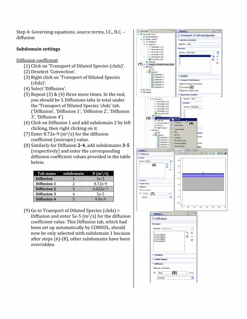
(1) Click on ‘Transport of Diluted Species (chds)’. (2) Deselect ‘Convection’. (3) Right click on ‘Transport of Diluted Species
(chds)’. (4) Select ‘Diffusion’. (5) Repeat (3) & (4) three more times. In the end,
you should be 5 Diffusions tabs in total under the ‘Transport of Diluted Species ‘chds’ tab. (‘Diffusion’, ‘Diffusion 1’, ‘Diffusion 2’, ‘Diffusion 3’, ‘Diffusion 4’)
(6) Click on Diffusion 1 and add subdomain 2 by left clicking, then right clicking on it.
(7) Enter 8.72e-9 (m2/s) for the diffusion coefficient (isotropic) value.
(8) Similarly for Diffusion 2-4, add subdomains 3-5 (respectively) and enter the corresponding diffusion coefficient values provided in the table below.
Diffusion and enter 5e-5 (m2/s) for the diffusion coefficient value. This Diffusion tab, which had been set up automatically by COMSOL, should now be only selected with subdomain 1 because after steps (6)-(8), other subdomains have been overridden.
Source term
(10)Right click on ‘Transport of Diluted Species (chds)’.
(11)Select ‘Reaction’. (12)Repeat (9) & (10) four more times. In the end,
you should be 5 Reactions tab in total. (‘Reactions 1-5’)
(13)Select Reactions 1 and add subdomain 1 by left clicking then right clicking on it.
(14)Enter -1e-4*c for Rc (mol/m3s). Similarly for other subdomains, enter the following values.
Initial Condition (15) Right click on ‘Transport of Diluted Species (chds)’. (16) Select ‘Initial Values’. (17) Click on ‘Initial Values 2’. (18) Left click, then right click on domain 5. (19) Enter 46.5 (mol/m3) for initial concentration
Boundary settings All boundaries have zero species flux, either due to symmetry (left boundaries) or insulation (right boundaries), or are considered to be semi-infinite (bottom boundary). Since the default boundary condition of the solver if zero flux, we retain the default settings.
Step 6: Solver setting and solution
(1) Click left of ‘Study 1’ to expand the option.
(2) Select ‘Step 1: Time Dependent’.
(3) Enter range (0,100,72000).
(4) Right click on ‘Study 1’.
(5) Select ‘Compute’.
Step 7: Postprocessing To generate the plot of drug lost from the lens and absorbed in the aqueous humor as functions of time:
(1) Right click on ‘Data Sets’.
(2) Select Evaluation > Integral.
(3) Repeat (1) & (2).
(4) Right click on ‘Integral 1’.
(5) Select ‘Add Selection’.
(6) Repeat (4) & (5) for ‘Integral 2’.
(7) Click on Integral 1 > Selection. Change the geometric entity level to ‘Domain’ and select subdomain 1 by left clicking, then right clicking on it.
(8) Click on Integral 2 > Selection. Change the geometric entity level to ‘Domain’ and select subdomain 5 by left clicking, then right clicking on it.
(9) Right click on ‘Results’.
(10)Select ‘1D Plot Group’.
(11)Repeat (9) & 10).
(12)Right click on ‘1D Plot Group 2’.
(13)Select ‘Global’.
(14)Repeat (12) & (13) for ‘1D Plot Group 3’.
(15)Click on 1D Plot Group 2 > Global 1 and select ‘Integral 1’ from the Data set drop-down menu.
(16)Click on the first row of the Expressions table.
(17)Click on the Expression edit field below the table and enter the expression: 2*pi*r*c
(18)Click ‘Plot’ icon.
(19)Click on 1D Plot Group 3 > Global 1 and select ‘Integral 2’ from the Data set drop-down menu.
(20)Click on the first row of the Expression table.
(21)Click on the Expression edit field below the table and and enter the expression: 2*pi*r*c
(22)Click ‘Plot’ icon.
This generates the following two figures.
To generate a plot of concentration of the drug on the surface of the lens as a function of time:
(1) Right click on ‘Data Sets’. (2) Select ‘Cut Point 2D’. (3) Enter 0 (m) for r and 0.2862 (m) for z. (4) Right click on ‘Results’. (5) Select ‘1D Plot Group’. (6) Right click on ‘1D Plot Group 4’. (7) Select ‘Point Graph’. (8) Select ‘Cut Point 2D 1’ under Data set drop-
down menu. (9) Click ‘Plot’ icon.
This generates the following figure.
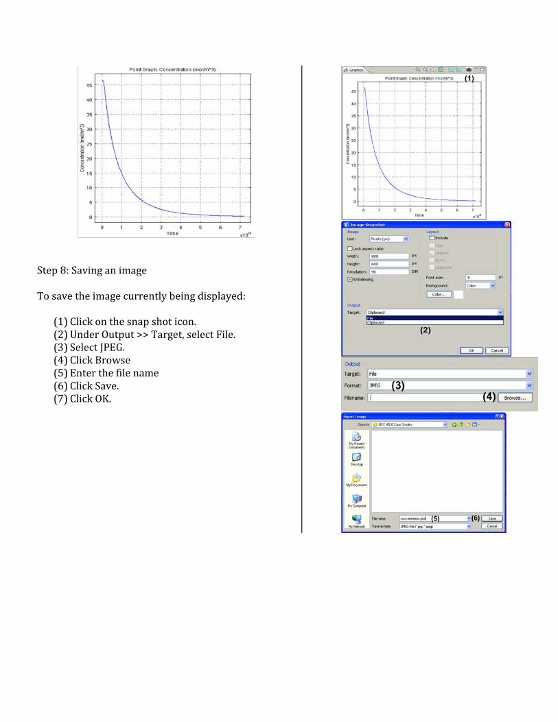
Step 8: Saving an image To save the image currently being displayed:
(1) Click on the snap shot icon. (2) Under Output >> Target, select File. (3) Select JPEG. (4) Click Browse (5) Enter the file name (6) Click Save. (7) Click OK.