20
Taming Statistics with Limited Domain Operators Stephen Mansour, PhD University of Scranton and The Carlisle Group Dyalog ’14 Conference, Eastbourne, UK
| Date post: | 14-Dec-2015 |
| Category: |
Documents |
| Upload: | teagan-jordison |
| View: | 216 times |
| Download: | 0 times |

Taming Statistics with Limited Domain Operators
Stephen Mansour, PhDUniversity of Scranton and The Carlisle Group
Dyalog ’14 Conference, Eastbourne, UK
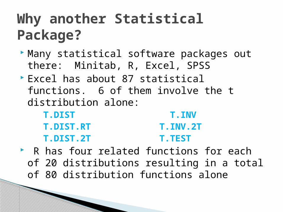
Many statistical software packages out there: Minitab, R, Excel, SPSS
Excel has about 87 statistical functions. 6 of them involve the t distribution alone:
T.DIST T.INVT.DIST.RT T.INV.2TT.DIST.2T T.TEST
R has four related functions for each of 20 distributions resulting in a total of 80 distribution functions alone
Why another Statistical Package?

Defined Operators!
How can we exploit operators to reduce the explosive number of statistical functions?
Let’s look at an example . . .
What does APL have that other Statistical package don’t?

Typical attendance is about 100 delegates with a standard deviation of 20.
Assume next year’s conference centre can support up to130 delegates.
What are the chances that next year’s attendance will exceed capacity?
Planning Next Year’s Conference User Meeting
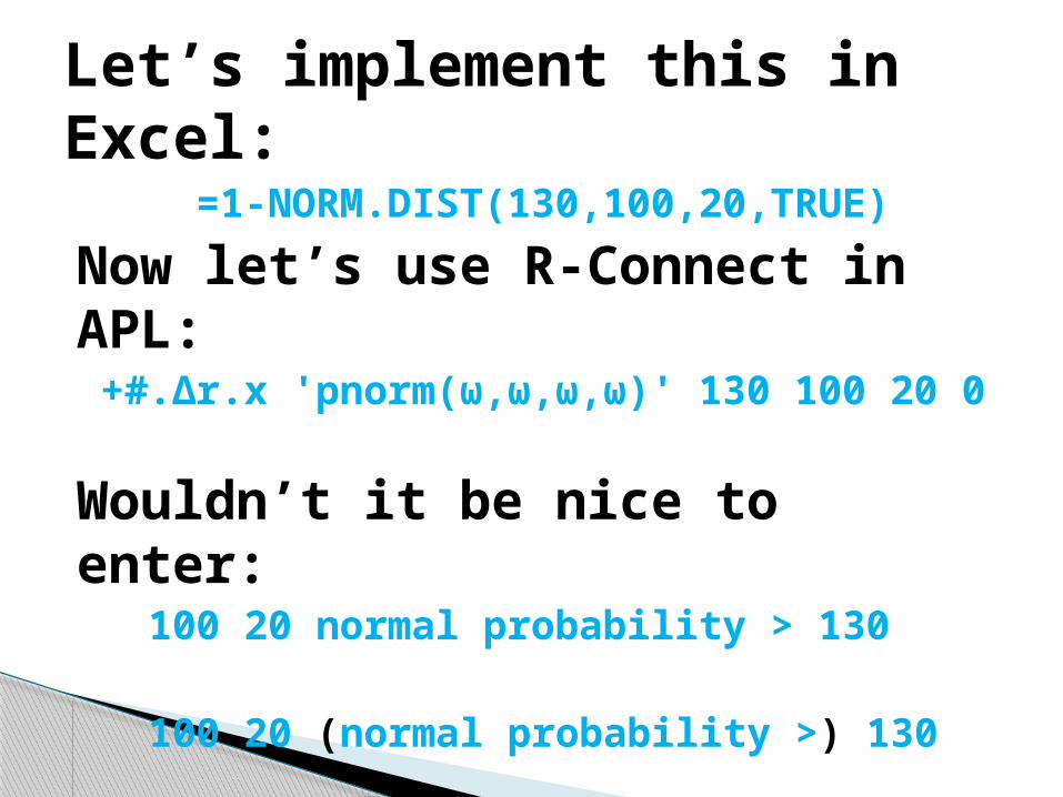
=1-NORM.DIST(130,100,20,TRUE)
Now let’s use R-Connect in APL: +#.∆r.x 'pnorm(⍵,⍵,⍵,⍵)' 130 100 20 0
Wouldn’t it be nice to enter: 100 20 normal probability > 130
100 20 (normal probability >) 130
Let’s implement this in Excel:

normal probability < 1.64100 20 normal probability between 110 1305 0.5 binomial probability = 27 tDist criticalValue < 0.055 chiSquare randomVariable 13mean confidenceInterval X(SEX='F') proportion hypothesis ≥ 0.5 GROUPA mean hypothesis = GROUPBvariance theoretical binomial 5 0.2
APL Syntax showingdata, functions, operators

Summary Functions ◦ Descriptive Statistics
Probability Distributions ◦ Theoretical Models
Relations
Statistics deals primarily with three types of functions:

Summary functions are of the form:
They produce a single value from a vector. Structurally they are equivalent to g/ where g is a scalar function and the right argument is a simple numeric vector. A statistic is a summary function of a sample; a parameter is a summary function of a population.
Summary Functions

Examples◦ Measures of central tendency:
mean, median, mode◦ Measures of Spread
variance, standard deviation, range , IQR◦ Measures of Position
min, max, quartiles, percentiles◦ Measures of shape
skewness, kurtosis
Examples of Summary Functions

Probability Distributions are functions defined in a natural way when they are called without an operator:◦ Discrete: probability mass function◦ Continuous: density function
Left argument is parameter list Right argument can be any value taken on
by the distribution. Probability Distributions are scalar with
respect to the right argument.
Probability Distributions
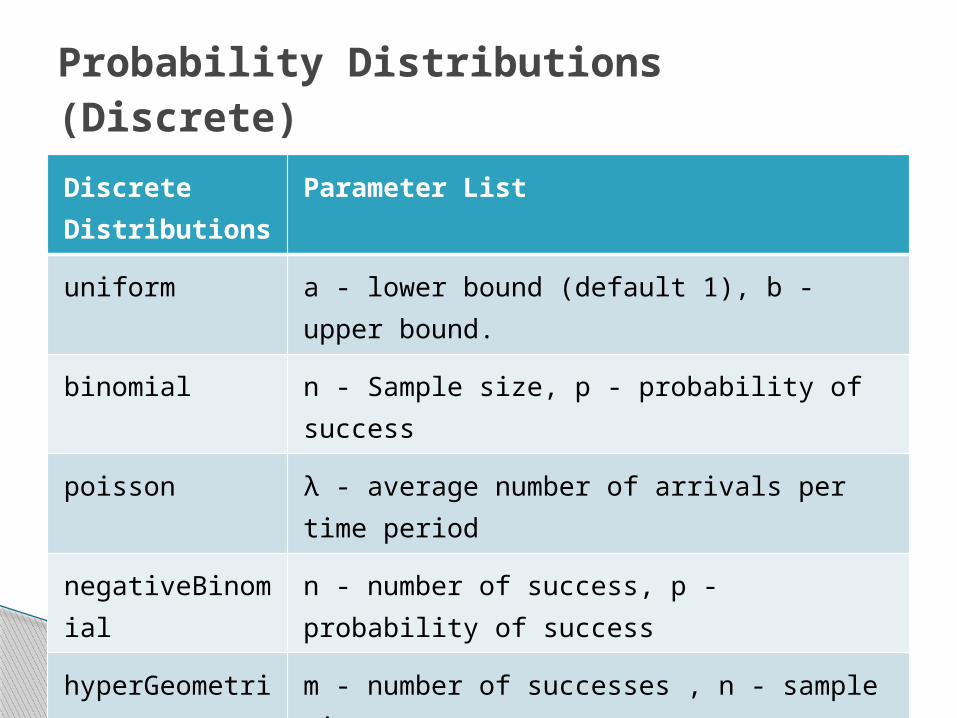
Discrete Distributions
Parameter List
uniform a - lower bound (default 1), b - upper bound.
binomial n - Sample size, p - probability of success
poisson λ - average number of arrivals per time period
negativeBinomial n - number of success, p - probability of success
hyperGeometric m - number of successes , n - sample size , N - Population size
multinomial V - List of Values (default 1 thru n), P - List of probabilities totaling 1
Probability Distributions (Discrete)

Continuous Distributions Parameter List
normal μ - theoretical mean (default 0); σ - standard deviation (default 1)
exponential λ - mean time to fail
rectangular (continuous uniform)
a - lower bound (default 0), b - upper bound (default 1)
triangular a - lower bound, m - most common value,b - upper bound
chiSquare df - degrees of freedom
tDist (Student) df - degrees of freedom
fDist df1 - degrees of freedom for numerator, df2 - degrees of freedom for denominator
Probability Distributions (Continuous)
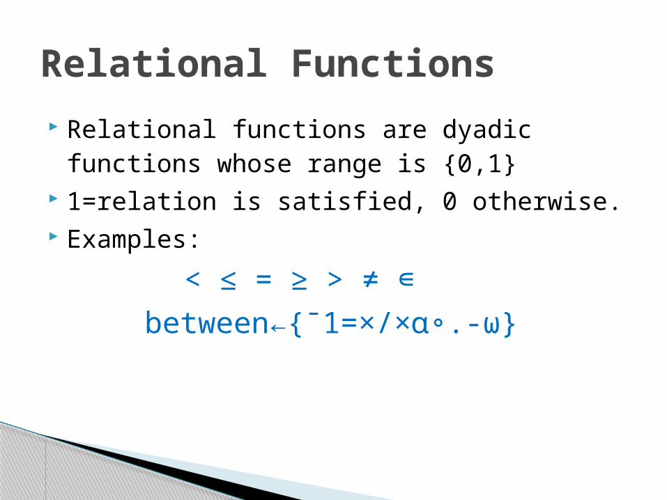
Relational functions are dyadic functions whose range is {0,1}
1=relation is satisfied, 0 otherwise. Examples:
< ≤ = ≥ > ≠ ∊ between←{¯1=×/×⍺∘.-⍵}
Relational Functions

By limiting the domain of an operator to one of the previously-defined functional classifications, we can create an operator to perform statistical analysis.
For a dyadic operator, each operand can be limited to a particular (but not necessarily the same) functional classification.
Limited-Domain Operators

Operator Left Operand
Right Operand
probability Distribution Relation
criticalValue Distribution Relation
confidenceInterval
Summary N/A
hypothesis Summary Relation
goodnessOfFit Distribution N/A
randomVariable Distribution N/A
theoretical Summary Distribution
running Summary N/A
Limited Domain Operators

Most functions and operators can easily be written in APL.
Internals not important to user R interface can be used if necessary for
statistical distributions. Correct nomenclature and ease of use is
critical.
This is about design and syntax, not implementation
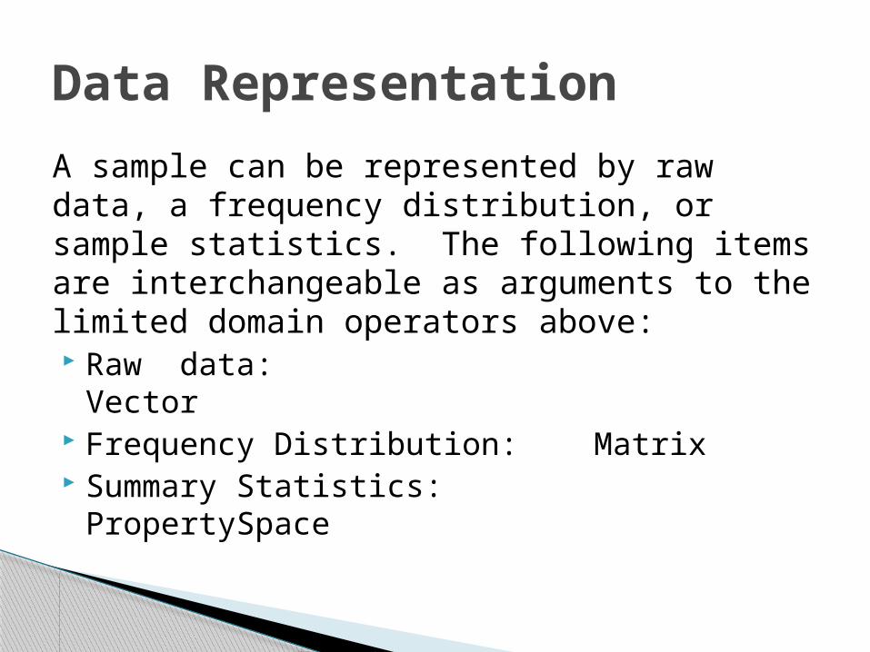
A sample can be represented by raw data, a frequency distribution, or sample statistics. The following items are interchangeable as arguments to the limited domain operators above: Raw data: Vector Frequency Distribution: Matrix Summary Statistics: PropertySpace
Data Representation
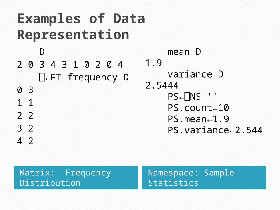
Examples of Data Representation
Matrix: Frequency Distribution
Namespace: Sample Statistics
D2 0 3 4 3 1 0 2 0 4 ⎕←FT←frequency D0 31 12 23 24 2
mean D1.9 variance D2.5444 PS←⎕NS '' PS.count←10 PS.mean←1.9 PS.variance←2.544
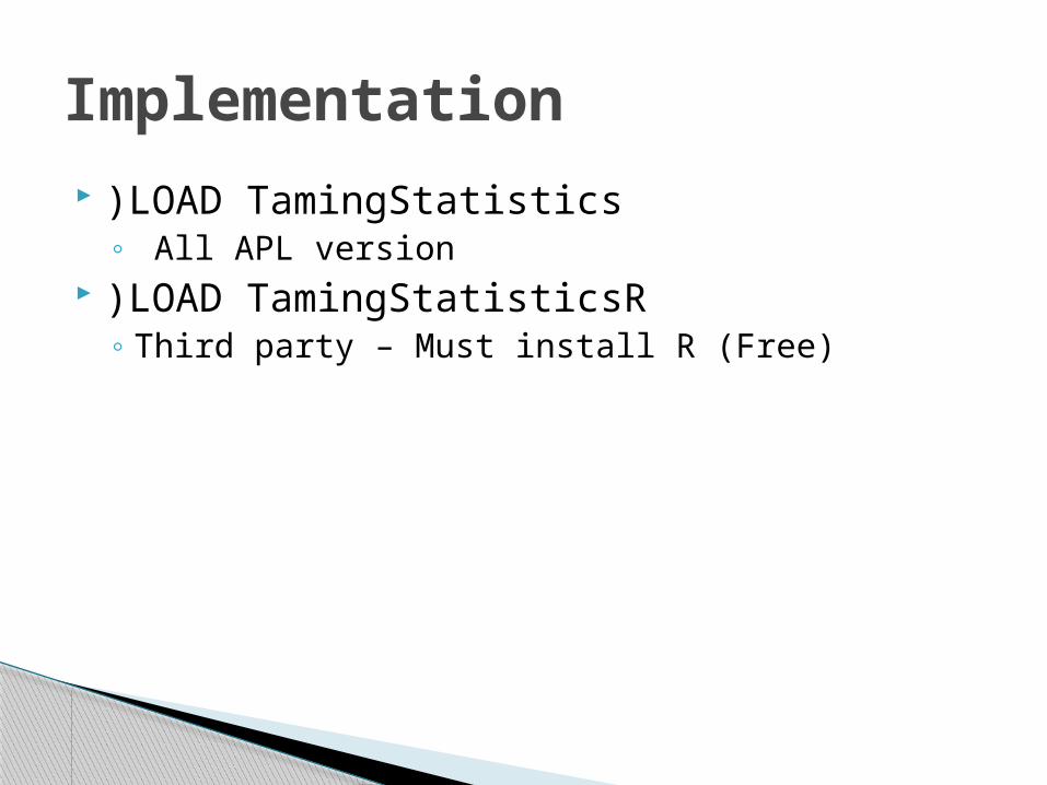
Implementation )LOAD TamingStatistics
◦ All APL version )LOAD TamingStatisticsR
◦ Third party – Must install R (Free)

There are many statistical packages out there; some, like R can be used with APL
Operator syntax is unique to APL R can be called directly from APL using
RCONNECT, but APL operator syntax is easier to understand.
Conclusion


