320
Undergraduate Texts in Mathematics Stephen Abbott Understanding Analysis Second Edition
| Date post: | 07-Aug-2019 |
| Category: |
Documents |
| Upload: | truongkhue |
| View: | 254 times |
| Download: | 16 times |

Undergraduate Texts in Mathematics
Stephen Abbott
Understanding Analysis Second Edition

Undergraduate Texts in Mathematics

Undergraduate Texts in Mathematics
Series Editors:
Sheldon AxlerSan Francisco State University, San Francisco, CA, USA
Kenneth RibetUniversity of California, Berkeley, CA, USA
Advisory Board:
Colin Adams, Williams CollegeDavid A. Cox, Amherst CollegePamela Gorkin, Bucknell UniversityRoger E. Howe, Yale UniversityMichael Orrison, Harvey Mudd CollegeJill Pipher, Brown UniversityFadil Santosa, University of Minnesota
Undergraduate Texts in Mathematics are generally aimed at third- and fourth-yearundergraduate mathematics students at North American universities. These texts striveto provide students and teachers with new perspectives and novel approaches. Thebooks include motivation that guides the reader to an appreciation of interrelationsamong different aspects of the subject. They feature examples that illustrate key con-cepts as well as exercises that strengthen understanding.
More information about this series at http://www.springer.com/series/666

Stephen Abbott
Understanding Analysis
Second Edition
123

Stephen AbbottDepartment of MathematicsMiddlebury CollegeMiddlebury, VT, USA
ISSN 0172-6056 ISSN 2197-5604 (electronic)Undergraduate Texts in MathematicsISBN 978-1-4939-2711-1 ISBN 978-1-4939-2712-8 (eBook)DOI 10.1007/978-1-4939-2712-8
Library of Congress Control Number: 2015937969
Mathematics Subject Classification (2010): 26-01
Springer New York Heidelberg Dordrecht London© Springer Science+Business Media New York 2001, 2015 (Corrected at 2nd printing 2016)This work is subject to copyright. All rights are reserved by the Publisher, whether the whole or part ofthe material is concerned, specifically the rights of translation, reprinting, reuse of illustrations, recitation,broadcasting, reproduction on microfilms or in any other physical way, and transmission or informationstorage and retrieval, electronic adaptation, computer software, or by similar or dissimilar methodology nowknown or hereafter developed.The use of general descriptive names, registered names, trademarks, service marks, etc. in this publicationdoes not imply, even in the absence of a specific statement, that such names are exempt from the relevantprotective laws and regulations and therefore free for general use.The publisher, the authors and the editors are safe to assume that the advice and information in this bookare believed to be true and accurate at the date of publication. Neither the publisher nor the authors or theeditors give a warranty, express or implied, with respect to the material contained herein or for any errors oromissions that may have been made.
Printed on acid-free paper
Springer Science+Business Media LLC New York is part of Springer Science+Business Media (www.springer.com)

Preface
My primary goal in writing Understanding Analysis was to create an elemen-tary one-semester book that exposes students to the rich rewards inherent intaking a mathematically rigorous approach to the study of functions of a realvariable. The aim of a course in real analysis should be to challenge and im-prove mathematical intuition rather than to verify it. There is a tendency,however, to center an introductory course too closely around the familiar the-orems of the standard calculus sequence. Producing a rigorous argument thatpolynomials are continuous is good evidence for a well-chosen definition of con-tinuity, but it is not the reason the subject was created and certainly not thereason it should be required study. By shifting the focus to topics where anuntrained intuition is severely disadvantaged (e.g., rearrangements of infiniteseries, nowhere-differentiable continuous functions, Cantor sets), my intent is tobring an intellectual liveliness to this course by offering the beginning studentaccess to some truly significant achievements of the subject.
The Main Objectives
Real analysis stands as a beacon of stability in the otherwise unpredictable evo-lution of the mathematics curriculum. Amid the various pedagogical revolutionsin calculus, computing, statistics, and data analysis, nearly every undergradu-ate program continues to require at least one semester of real analysis. Myown department once challenged this norm by creating a mathematical sciencestrack that allowed students to replace our two core proof-writing classes withelectives in departments like physics and computer science. Within a few years,however, we concluded that the pieces did not hold together without a course inanalysis. Analysis is, at once, a course in philosophy and applied mathematics.It is abstract and axiomatic in nature, but is engaged with the mathematicsused by economists and engineers.
How then do we teach a successful course to students with such diverseinterests and expectations? Our desire to make analysis required study for wideraudiences must be reconciled with the fact that many students find the subjectquite challenging and even a bit intimidating. One unfortunate resolution of this
v

vi Preface
dilemma is to make the course easier by making it less interesting. The omittedmaterial is inevitably what gives analysis its true flavor. A better solution is tofind a way to make the more advanced topics accessible and worth the effort.
I see three essential goals that a semester of real analysis should try to meet:
1. Students need to be confronted with questions that expose the insufficiencyof an informal understanding of the objects of calculus. The need for amore rigorous study should be carefully motivated.
2. Having seen mainly intuitive or heuristic arguments, students need to learnwhat constitutes a rigorous mathematical proof and how to write one.
3. Most importantly, there needs to be significant reward for the difficultwork of firming up the logical structure of limits. Specifically, real anal-ysis should not be just an elaborate reworking of standard introductorycalculus. Students should be exposed to the tantalizing complexities ofthe real line, to the subtleties of different flavors of convergence, and tothe intellectual delights hidden in the paradoxes of the infinite.
The philosophy of Understanding Analysis is to focus attention on questionsthat give analysis its inherent fascination. Does the Cantor set contain anyirrational numbers? Can the set of points where a function is discontinuousbe arbitrary? Are derivatives continuous? Are derivatives integrable? Is aninfinitely differentiable function necessarily the limit of its Taylor series? Ingiving these topics center stage, the hard work of a rigorous study is justifiedby the fact that they are inaccessible without it.
The Audience
This book is an introductory text. The only prerequisite is a robust understand-ing of the results from single-variable calculus. The theorems of linear algebraare not needed, but the exposure to abstract arguments and proof writing thatusually comes with this course would be a valuable asset. Complex numbers arenever used.
The proofs in Understanding Analysis are written with the beginning studentfirmly in mind. Brevity and other stylistic concerns are postponed in favorof including a significant level of detail. Most proofs come with a generousamount of discussion about the context of the argument. What should theproof entail? Which definitions are relevant? What is the overall strategy?Whenever there is a choice, efficiency is traded for an opportunity to reinforcesome previously learned technique. Especially familiar or predictable argumentsare often deferred to the exercises.
The search for recurring ideas exists at the proof-writing level and also onthe larger expository level. I have tried to give the course a narrative tone bypicking up on the unifying themes of approximation and the transition from thefinite to the infinite. Often when we ask a question in analysis the answer is

Preface vii
“sometimes.” Can the order of a double summation be exchanged? Is term-by-term differentiation of an infinite series allowed? By focusing on this recurringpattern, each successive topic builds on the intuition of the previous one. Thequestions seem more natural, and a coherent story emerges from what mightotherwise appear as a long list of theorems and proofs.
This book always emphasizes core ideas over generality, and it makes noeffort to be a complete, deductive catalog of results. It is designed to capture theintellectual imagination. Those who become interested are then exceptionallywell prepared for a second course starting from complex-valued functions onmore general spaces, while those content with a single semester come away witha strong sense of the essence and purpose of real analysis.
The Structure of the Book
Although the book finds its way to some sophisticated results, the main bodyof each chapter consists of a lean and focused treatment of the core topicsthat make up the center of most courses in analysis. Fundamental results aboutcompleteness, compactness, sequential and functional limits, continuity, uniformconvergence, differentiation, and integration are all incorporated.
What is specific here is where the emphasis is placed. In the chapter on inte-gration, for instance, the exposition revolves around deciphering the relationshipbetween continuity and the Riemann integral. Enough properties of the integralare obtained to justify a proof of the Fundamental Theorem of Calculus, butthe theme of the chapter is the pursuit of a characterization of integrable func-tions in terms of continuity. Whether or not Lebesgue’s measure-zero criterionis treated, framing the material in this way is still valuable because it is thequestions that are important. Mathematics is not a static discipline. Studentsshould be aware of the historical reasons for the creation of the mathematicsthey are learning and by extension realize that there is no last word on thesubject. In the case of integration, this point is made explicitly by includingsome relatively modern developments on the generalized Riemann integral inthe additional topics of the last chapter.
The structure of the chapters has the following distinctive features.
Discussion Sections: Each chapter begins with the discussion of some mo-tivating examples and open questions. The tone in these discussions is inten-tionally informal, and full use is made of familiar functions and results fromcalculus. The idea is to freely explore the terrain, providing context for theupcoming definitions and theorems. After these exploratory introductions, thetone of the writing changes, and the treatment becomes rigorously tight butstill not overly formal. With the questions in place, the need for the ensuingdevelopment of the material is well motivated and the payoff is in sight.
Project Sections: The penultimate section of each chapter (the final section isa short epilogue) is written with the exercises incorporated into the exposition.Proofs are outlined but not completed, and additional exercises are included toelucidate the material being discussed. The sections are written as self-guided

viii Preface
tutorials, but they can also be the subject of lectures. I typically use them inplace of a final examination, and they work especially well as collaborative as-signments that can culminate in a class presentation. The body of each chaptercontains the necessary tools, so there is some satisfaction in letting the studentsuse their newly acquired skills to ferret out for themselves answers to questionsthat have been driving the exposition.
Building a Course
Although this book was originally designed for a 12–14-week semester, it hasbeen used successfully in any number of formats including independent study.The dependence of the sections follows the natural ordering, but there is someflexibility as to what can be treated and omitted.
• The introductory discussions to each chapter can be the subject of lecture,assigned as reading, omitted, or substituted with something preferable.There are no theorems proved here that show up later in the text. I dodevelop some important examples in these introductions (the Cantor set,Dirichlet’s nowhere-continuous function) that probably need to find theirway into discussions at some point.
• Chapter 3, Basic Topology of R, is much longer than it needs to be. Allthat is required by the ensuing chapters are fundamental results aboutopen and closed sets and a thorough understanding of sequential com-pactness. The characterization of compactness using open covers as wellas the section on perfect and connected sets are included for their own in-trinsic interest. They are not, however, crucial to any future proofs. Theone exception to this is a presentation of the Intermediate Value Theorem(IVT) as a special case of the preservation of connected sets by continu-ous functions. To keep connectedness truly optional, I have included twodirect proofs of IVT based on completeness results from Chapter 1.
• All the project sections (1.6, 2.8, 3.5, 4.6, 5.4, 6.7, 7.6, 8.1–8.6) are optionalin the sense that no results in later chapters depend on material in thesesections. The six topics covered in Chapter 8 are also written in thistutorial-style format, where the exercises make up a significant part of thedevelopment. The only one of these sections that might benefit from alecture is the unit on Fourier series, which is a bit longer than the others.
Changes in the Second Edition
In light of the encouraging feedback—especially from students—I decided notto attempt any major alterations to the central narrative of the text as it wasset out in the original edition. Some longer sections have been edited down,or in one case split in two, and the unit on Taylor series is now part of the

Preface ix
core material of Chapter 6 instead of being relegated to the closing projectsection. In contrast to the main body of the book, significant effort has goneinto revising the exercises and projects. There are roughly 150 new exercises inthis edition alongside 200 or so of what I feel are the most effective problemsfrom the first edition. Some of these introduce new ideas not covered in thechapters (e.g., Euler’s constant, infinite products, inverse functions), but themajority are designed to kindle debates about the major ideas under discussionin what I hope are engaging ways. There are ample propositions to prove butalso a good supply of Moore-method type exercises that require assessing thevalidity of various conjectures, deciphering invented definitions, or searching forexamples that may not exist.
The introductory discussion to Chapter 6 is new and tells the story of howEuler’s deft and audacious manipulations of power series led to a computationof
∑1/n2. Providing a proper proof for Euler’s sum is the topic of one of
three new project sections. The other two are a treatment of the WeierstrassApproximation Theorem and an exploration of how to best extend the domain ofthe factorial function to all of R. Each of these three topics represents a seminalachievement in the history of analysis, but my decision to include them has asmuch to do with the associated ideas that accompany the main proofs. For theWeierstrass Approximation Theorem, the particular argument that I chose relieson Taylor series and a deep understanding of uniform convergence, making itan ideal project to conclude Chapter 6. The journey to a proper definition of x!allowed me to include a short unit on improper integrals and a proof of Leibniz’srule for differentiating under the integral sign. The accompanying topics for theproject on Euler’s sum are an analysis of the integral remainder formula forTaylor series and a proof of Wallis’s famous product formula for π. Yes theseare challenging arguments but they are also beautiful ideas. Returning to thethesis of this text, it is my conviction that encounters with results like thesemake the task of learning analysis less daunting and more meaningful. Theymake the epsilons matter.
Acknowledgements
I never met Robert Bartle, although it seems like I did. As a student and ayoung professor, I spent many hours learning and teaching analysis from hisbooks. I did eventually correspond with him back in 2000 while working onthe first edition of this text because I wanted to include a project based on hisarticle, “Return to the Riemann Integral.” Professor Bartle was gracious andhelpful, even though he was editing his own competing text to include the samematerial. In September 2003, Robert Bartle died following a long battle withcancer at the age of 76. The section his article inspired on the GeneralizedRiemann integral continues to be one of my favorite projects to assign, but it isfair to say that Professor Bartle’s lucid mathematical writing has been a sourceof inspiration for the entire text.

x Preface
My long and winding journey to find an elegant proof of Euler’s sum con-structed only from theorems in the first seven chapters in this text came toa happy conclusion in Peter Duren’s recently published Invitation to ClassicalAnalysis. A treasure trove of fascinating topics that have been largely excisedfrom the undergraduate curriculum, Duren’s book is remarkable in part for howmuch he accomplishes without the use of Lebesgue’s theory. T.W. Korner’swonderfully opinionated A Companion to Analysis is another engaging readthat inspired a few of the new exercises in this edition. Analysis by Its History,by E. Hairer and G. Wanner, and A Radical Approach to Real Analysis, byDavid Bressoud, were both cited in the acknowledgements of the first edition assources for many of the historical anecdotes that permeate the text. Since then,Professor Bressoud has published a sequel, A Radical Approach to Lebesgue’sTheory of Integration, which I heartily recommend.
The significant contributions of Benjamin Lotto, Loren Pitt, and Paul Humketo the content of the first edition warrant a second nod in these acknowledge-ments. As for the new edition, Dan Velleman taught from a draft of the textand provided much helpful feedback. Whatever problems still remain are likelyplaces where I stubbornly did not follow Dan’s advice. Back in 2001, SteveKennedy penned a review of Understanding Analysis which I am sure enhancedthe audience for this book. His kind assessment nevertheless included a numberof worthy suggestions for improvement, most of which I have incorporated. Ishould also acknowledge Fernando Gouvea as the one who suggested that theseries of articles by David Fowler on the factorial function would fit well withthe themes of this book. The result is Section 8.4.
I would like to express my continued appreciation to the staff at Springer, andin particular to Marc Strauss and Eugene Ha for their support and unwaveringfaith in the merits of this project. The large email file of thoughtful suggestionsfrom users of the book is too long to enumerate, but perhaps this is the placeto say that I continue to welcome comments from readers, even moderatelydisgruntled ones. The most gratifying aspect of authoring the first edition isthe sense of being connected to the larger mathematical community and of beingan active participant in it.
The margins of my original copy of Understanding Analysis are filled withvestiges of my internal debates about what to revise, what to preserve, and whatto discard. The final decisions I made are the result of 15 years of classroomexperiments with the text, and it is comforting to report that the main bodyof the book has weathered the test of time with only a modest tune-up. On asimilarly positive note, the original dedication of this book to my wife Katy isanother feature of the first edition that has required no additional editing.
Middlebury, VT, USA Stephen AbbottMarch 2015

Contents
1 The Real Numbers 11.1 Discussion: The Irrationality of
√2 . . . . . . . . . . . . . . . . . 1
1.2 Some Preliminaries . . . . . . . . . . . . . . . . . . . . . . . . . . 51.3 The Axiom of Completeness . . . . . . . . . . . . . . . . . . . . . 141.4 Consequences of Completeness . . . . . . . . . . . . . . . . . . . 201.5 Cardinality . . . . . . . . . . . . . . . . . . . . . . . . . . . . . . 251.6 Cantor’s Theorem . . . . . . . . . . . . . . . . . . . . . . . . . . 321.7 Epilogue . . . . . . . . . . . . . . . . . . . . . . . . . . . . . . . . 36
2 Sequences and Series 392.1 Discussion: Rearrangements of Infinite Series . . . . . . . . . . . 392.2 The Limit of a Sequence . . . . . . . . . . . . . . . . . . . . . . . 422.3 The Algebraic and Order Limit Theorems . . . . . . . . . . . . . 492.4 The Monotone Convergence Theorem and a First Look at
Infinite Series . . . . . . . . . . . . . . . . . . . . . . . . . . . . . 562.5 Subsequences and the Bolzano–Weierstrass Theorem . . . . . . . 622.6 The Cauchy Criterion . . . . . . . . . . . . . . . . . . . . . . . . 662.7 Properties of Infinite Series . . . . . . . . . . . . . . . . . . . . . 712.8 Double Summations and Products of Infinite Series . . . . . . . . 792.9 Epilogue . . . . . . . . . . . . . . . . . . . . . . . . . . . . . . . . 83
3 Basic Topology of R 853.1 Discussion: The Cantor Set . . . . . . . . . . . . . . . . . . . . . 853.2 Open and Closed Sets . . . . . . . . . . . . . . . . . . . . . . . . 883.3 Compact Sets . . . . . . . . . . . . . . . . . . . . . . . . . . . . . 963.4 Perfect Sets and Connected Sets . . . . . . . . . . . . . . . . . . 1023.5 Baire’s Theorem . . . . . . . . . . . . . . . . . . . . . . . . . . . 1063.6 Epilogue . . . . . . . . . . . . . . . . . . . . . . . . . . . . . . . . 109
4 Functional Limits and Continuity 1114.1 Discussion: Examples of Dirichlet and Thomae . . . . . . . . . . 1114.2 Functional Limits . . . . . . . . . . . . . . . . . . . . . . . . . . . 115
xi

xii Contents
4.3 Continuous Functions . . . . . . . . . . . . . . . . . . . . . . . . 1224.4 Continuous Functions on Compact Sets . . . . . . . . . . . . . . 1294.5 The Intermediate Value Theorem . . . . . . . . . . . . . . . . . . 1364.6 Sets of Discontinuity . . . . . . . . . . . . . . . . . . . . . . . . . 1414.7 Epilogue . . . . . . . . . . . . . . . . . . . . . . . . . . . . . . . . 144
5 The Derivative 1455.1 Discussion: Are Derivatives Continuous? . . . . . . . . . . . . . . 1455.2 Derivatives and the Intermediate Value Property . . . . . . . . . 1485.3 The Mean Value Theorems . . . . . . . . . . . . . . . . . . . . . 1555.4 A Continuous Nowhere-Differentiable Function . . . . . . . . . . 1625.5 Epilogue . . . . . . . . . . . . . . . . . . . . . . . . . . . . . . . . 166
6 Sequences and Series of Functions 1696.1 Discussion: The Power of Power Series . . . . . . . . . . . . . . . 1696.2 Uniform Convergence of a Sequence of Functions . . . . . . . . . 1736.3 Uniform Convergence and Differentiation . . . . . . . . . . . . . 1846.4 Series of Functions . . . . . . . . . . . . . . . . . . . . . . . . . . 1886.5 Power Series . . . . . . . . . . . . . . . . . . . . . . . . . . . . . . 1916.6 Taylor Series . . . . . . . . . . . . . . . . . . . . . . . . . . . . . 1976.7 The Weierstrass Approximation Theorem . . . . . . . . . . . . . 2056.8 Epilogue . . . . . . . . . . . . . . . . . . . . . . . . . . . . . . . . 211
7 The Riemann Integral 2157.1 Discussion: How Should Integration be Defined? . . . . . . . . . 2157.2 The Definition of the Riemann Integral . . . . . . . . . . . . . . . 2187.3 Integrating Functions with Discontinuities . . . . . . . . . . . . . 2247.4 Properties of the Integral . . . . . . . . . . . . . . . . . . . . . . 2287.5 The Fundamental Theorem of Calculus . . . . . . . . . . . . . . . 2347.6 Lebesgue’s Criterion for Riemann Integrability . . . . . . . . . . 2387.7 Epilogue . . . . . . . . . . . . . . . . . . . . . . . . . . . . . . . . 246
8 Additional Topics 2498.1 The Generalized Riemann Integral . . . . . . . . . . . . . . . . . 2498.2 Metric Spaces and the Baire Category Theorem . . . . . . . . . . 2588.3 Euler’s Sum . . . . . . . . . . . . . . . . . . . . . . . . . . . . . . 2648.4 Inventing the Factorial Function . . . . . . . . . . . . . . . . . . 2708.5 Fourier Series . . . . . . . . . . . . . . . . . . . . . . . . . . . . . 2818.6 A Construction of R From Q . . . . . . . . . . . . . . . . . . . . 297
Bibliography 305
Index 307

Chapter 1
The Real Numbers
1.1 Discussion: The Irrationality of√2
Toward the end of his distinguished career, the renowned British mathematicianG.H. Hardy eloquently laid out a justification for a life of studying mathematicsin A Mathematician’s Apology, an essay first published in 1940. At the centerof Hardy’s defense is the thesis that mathematics is an aesthetic discipline. ForHardy, the applied mathematics of engineers and economists held little charm.“Real mathematics,” as he referred to it, “must be justified as art if it can bejustified at all.”
To help make his point, Hardy includes two theorems from classical Greekmathematics, which, in his opinion, possess an elusive kind of beauty that,although difficult to define, is easy to recognize. The first of these results isEuclid’s proof that there are an infinite number of prime numbers. The secondresult is the discovery, attributed to the school of Pythagoras from around 500B.C., that
√2 is irrational. It is this second theorem that demands our attention.
(A course in number theory would focus on the first.) The argument uses onlyarithmetic, but its depth and importance cannot be overstated. As Hardy says,“[It] is a ‘simple’ theorem, simple both in idea and execution, but there is nodoubt at all about [it being] of the highest class. [It] is as fresh and significant aswhen it was discovered—two thousand years have not written a wrinkle on [it].”
Theorem 1.1.1. There is no rational number whose square is 2.
Proof. A rational number is any number that can be expressed in the form p/q,where p and q are integers. Thus, what the theorem asserts is that no matterhow p and q are chosen, it is never the case that (p/q)
2= 2. The line of attack
is indirect, using a type of argument referred to as a proof by contradiction.The idea is to assume that there is a rational number whose square is 2 andthen proceed along logical lines until we reach a conclusion that is unacceptable.
© Springer Science+Business Media New York 2015S. Abbott, Understanding Analysis, Undergraduate Textsin Mathematics, DOI 10.1007/978-1-4939-2712-8 1
1

2 Chapter 1. The Real Numbers
At this point, we will be forced to retrace our steps and reject the erroneousassumption that some rational number squared is equal to 2. In short, we willprove that the theorem is true by demonstrating that it cannot be false.
And so assume, for contradiction, that there exist integers p and q satisfying
(1)
(p
q
)2
= 2.
We may also assume that p and q have no common factor, because, if they hadone, we could simply cancel it out and rewrite the fraction in lowest terms. Now,equation (1) implies
(2) p2 = 2q2.
From this, we can see that the integer p2 is an even number (it is divisible by 2),and hence p must be even as well because the square of an odd number is odd.This allows us to write p = 2r, where r is also an integer. If we substitute 2rfor p in equation (2), then a little algebra yields the relationship
2r2 = q2.
But now the absurdity is at hand. This last equation implies that q2 is even,and hence q must also be even. Thus, we have shown that p and q are botheven (i.e., divisible by 2) when they were originally assumed to have no commonfactor. From this logical impasse, we can only conclude that equation (1) cannothold for any integers p and q, and thus the theorem is proved.
A component of Hardy’s definition of beauty in a mathematical theoremis that the result have lasting and serious implications for a network of othermathematical ideas. In this case, the ideas under assault were the Greeks’ under-standing of the relationship between geometric length and arithmetic number.Prior to the preceding discovery, it was an assumed and commonly used factthat, given two line segments AB and CD, it would always be possible to finda third line segment whose length divides evenly into the first two. In modernterminology, this is equivalent to asserting that the length of CD is a rationalmultiple of the length of AB. Looking at the diagonal of a unit square (Fig. 1.1),it now followed (using the Pythagorean Theorem) that this was not always thecase. Because the Pythagoreans implicitly interpreted number to mean rationalnumber, they were forced to accept that number was a strictly weaker notionthan length.
Rather than abandoning arithmetic in favor of geometry (as the Greeks seemto have done), our resolution to this limitation is to strengthen the concept ofnumber by moving from the rational numbers to a larger number system. Froma modern point of view, this should seem like a familiar and somewhat naturalphenomenon. We begin with the natural numbers
N = {1, 2, 3, 4, 5, . . .}.

1.1. Discussion: The Irrationality of√2 3
CA B
D
1
1
√2
Figure 1.1:√2 exists as a geometric length.
The influential German mathematician Leopold Kronecker (1823–1891) onceasserted that “The natural numbers are the work of God. All of the rest isthe work of mankind.” Debating the validity of this claim is an interestingconversation for another time. For the moment, it at least provides us witha place to start. If we restrict our attention to the natural numbers N, thenwe can perform addition perfectly well, but we must extend our system to theintegers
Z = {. . . ,−3,−2,−1, 0, 1, 2, 3, . . .}if we want to have an additive identity (zero) and the additive inverses necessaryto define subtraction. The next issue is multiplication and division. The number1 acts as the multiplicative identity, but in order to define division we need tohave multiplicative inverses. Thus, we extend our system again to the rationalnumbers
Q =
{
all fractionsp
qwhere p and q are integers with q �= 0
}
.
Taken together, the properties of Q discussed in the previous paragraphessentially make up the definition of what is called a field . More formally stated,a field is any set where addition and multiplication are well-defined operationsthat are commutative, associative, and obey the familiar distributive propertya(b+ c) = ab+ ac. There must be an additive identity, and every element musthave an additive inverse. Finally, there must be a multiplicative identity, andmultiplicative inverses must exist for all nonzero elements of the field. NeitherZ nor N is a field. The finite set {0, 1, 2, 3, 4} is a field when addition andmultiplication are computed modulo 5. This is not immediately obvious butmakes an interesting exercise.
The set Q also has a natural order defined on it. Given any two rationalnumbers r and s, exactly one of the following is true:
r < s, r = s, or r > s.

4 Chapter 1. The Real Numbers
11.414
√2
1.5 2↑↓
Figure 1.2: Approximating√2 with rational numbers.
This ordering is transitive in the sense that if r < s and s < t, then r < t, sowe are conveniently led to a mental picture of the rational numbers as beinglaid out from left to right along a number line. Unlike Z, there are no intervalsof empty space. Given any two rational numbers r < s, the rational number(r+s)/2 sits halfway in between, implying that the rational numbers are denselynestled together.
With the field properties of Q allowing us to safely carry out the algebraicoperations of addition, subtraction, multiplication, and division, let’s remindourselves just what it is that Q is lacking. By Theorem 1.1.1, it is apparentthat we cannot always take square roots. The problem, however, is actuallymore fundamental than this. Using only rational numbers, it is possible toapproximate
√2 quite well (Fig. 1.2). For instance, 1.4142 = 1.999396. By
adding more decimal places to our approximation, we can get even closer toa value for
√2, but, even so, we are now well aware that there is a “hole” in
the rational number line where√2 ought to be. Of course, there are quite a
few other holes—at√3 and
√5, for example. Returning to the dilemma of the
ancient Greek mathematicians, if we want every length along the number line tocorrespond to an actual number, then another extension to our number systemis in order. Thus, to the chain N ⊆ Z ⊆ Q we append the real numbers R.
The question of how to actually construct R from Q is rather complicatedbusiness. It is discussed in Section 1.3, and then again in more detail in Sec-tion 8.6. For the moment, it is not too inaccurate to say that R is obtained byfilling in the gaps in Q. Wherever there is a hole, a new irrational number isdefined and placed into the ordering that already exists on Q. The real numbersare then the union of these irrational numbers together with the more familiarrational ones. What properties does the set of irrational numbers have? Howdo the sets of rational and irrational numbers fit together? Is there a kind ofsymmetry between the rationals and the irrationals, or is there some sense inwhich we can argue that one type of real number is more common than theother? The one method we have seen so far for generating examples of irra-tional numbers is through square roots. Not too surprisingly, other roots suchas 3
√2 or 5
√3 are most often irrational. Can all irrational numbers be expressed
as algebraic combinations of nth roots and rational numbers, or are there stillother irrational numbers beyond those of this form?

1.2. Some Preliminaries 5
1.2 Some Preliminaries
The vocabulary necessary for the ensuing development comes from set theoryand the theory of functions. This should be familiar territory, but a brief reviewof the terminology is probably a good idea, if only to establish some agreed-uponnotation.
Sets
Intuitively speaking, a set is any collection of objects. These objects are referredto as the elements of the set. For our purposes, the sets in question will mostoften be sets of real numbers, although we will also encounter sets of functionsand, on a few occasions, sets whose elements are other sets.
Given a set A, we write x ∈ A if x (whatever it may be) is an element of A.If x is not an element of A, then we write x /∈ A. Given two sets A and B, theunion is written A ∪B and is defined by asserting that
x ∈ A ∪B provided that x ∈ A or x ∈ B (or potentially both).
The intersection A ∩B is the set defined by the rule
x ∈ A ∩B provided x ∈ A and x ∈ B.
Example 1.2.1. (i) There are many acceptable ways to assert the contentsof a set. In the previous section, the set of natural numbers was definedby listing the elements: N = {1, 2, 3, . . .}.
(ii) Sets can also be described in words. For instance, we can define the set Eto be the collection of even natural numbers.
(iii) Sometimes it is more efficient to provide a kind of rule or algorithm fordetermining the elements of a set. As an example, let
S = {r ∈ Q : r2 < 2}.
Read aloud, the definition of S says, “Let S be the set of all rationalnumbers whose squares are less than 2.” It follows that 1 ∈ S, 4/3 ∈ S,but 3/2 /∈ S because 9/4 ≥ 2.
Using the previously defined sets to illustrate the operations of intersectionand union, we observe that
N ∪ E = N, N ∩ E = E, N ∩ S = {1}, and E ∩ S = ∅.
The set ∅ is called the empty set and is understood to be the set that con-tains no elements. An equivalent statement would be to say that E and S aredisjoint .

6 Chapter 1. The Real Numbers
A word about the equality of two sets is in order (since we have just used thenotion). The inclusion relationship A ⊆ B or B ⊇ A is used to indicate thatevery element of A is also an element of B. In this case, we say A is a subset ofB, or B contains A. To assert that A = B means that A ⊆ B and B ⊆ A. Putanother way, A and B have exactly the same elements.
Quite frequently in the upcoming chapters, we will want to apply the unionand intersection operations to infinite collections of sets.
Example 1.2.2. Let
A1 = N = {1, 2, 3, . . .},A2 = {2, 3, 4, . . .},A3 = {3, 4, 5, . . .},
and, in general, for each n ∈ N, define the set
An = {n, n+ 1, n+ 2, . . .}.The result is a nested chain of sets
A1 ⊇ A2 ⊇ A3 ⊇ A4 ⊇ · · · ,where each successive set is a subset of all the previous ones. Notationally,
∞⋃
n=1
An,⋃
n∈N
An, or A1 ∪ A2 ∪A3 ∪ · · ·
are all equivalent ways to indicate the set whose elements consist of any elementthat appears in at least one particular An. Because of the nested property ofthis particular collection of sets, it is not too hard to see that
∞⋃
n=1
An = A1.
The notion of intersection has the same kind of natural extension to infinitecollections of sets. For this example, we have
∞⋂
n=1
An = ∅.
Let’s be sure we understand why this is the case. Suppose we had some naturalnumber m that we thought might actually satisfy m ∈ ⋂∞
n=1 An. What thiswould mean is that m ∈ An for every An in our collection of sets. Because mis not an element of Am+1, no such m exists and the intersection is empty.
As mentioned, most of the sets we encounter will be sets of real numbers.Given A ⊆ R, the complement of A, written Ac, refers to the set of all elementsof R not in A. Thus, for A ⊆ R,
Ac = {x ∈ R : x /∈ A}.

1.2. Some Preliminaries 7
A few times in our work to come, we will refer to De Morgan’s Laws, whichstate that
(A ∩B)c = Ac ∪Bc and (A ∪B)c = Ac ∩Bc.
Proofs of these statements are discussed in Exercise 1.2.5.Admittedly, there is something imprecise about the definition of set pre-
sented at the beginning of this discussion. The defining sentence begins withthe phrase “Intuitively speaking,” which might seem an odd way to embark on acourse of study that purportedly intends to supply a rigorous foundation for thetheory of functions of a real variable. In some sense, however, this is unavoid-able. Each repair of one level of the foundation reveals something below it inneed of attention. The theory of sets has been subjected to intense scrutiny overthe past century precisely because so much of modern mathematics rests on thisfoundation. But such a study is really only advisable once it is understood whyour naive impression about the behavior of sets is insufficient. For the directionin which we are heading, this will not happen, although an indication of somepotential pitfalls is given in Section 1.7.
Functions
Definition 1.2.3. Given two sets A and B, a function from A to B is a rule ormapping that takes each element x ∈ A and associates with it a single elementof B. In this case, we write f : A → B. Given an element x ∈ A, the expressionf(x) is used to represent the element of B associated with x by f . The set A iscalled the domain of f . The range of f is not necessarily equal to B but refersto the subset of B given by {y ∈ B : y = f(x) for some x ∈ A}.
This definition of function is more or less the one proposed by Peter LejeuneDirichlet (1805–1859) in the 1830s. Dirichlet was a German mathematician whowas one of the leaders in the development of the rigorous approach to functionsthat we are about to undertake. His main motivation was to unravel the issuessurrounding the convergence of Fourier series. Dirichlet’s contributions figureprominently in Section 8.5, where an introduction to Fourier series is presented,but we will also encounter his name in several earlier chapters along the way.What is important at the moment is that we see how Dirichlet’s definitionof function liberates the term from its interpretation as a type of “formula.”In the years leading up to Dirichlet’s time, the term “function” was generallyunderstood to refer to algebraic entities such as f(x) = x2+1 or g(x) =
√x4 + 4.
Definition 1.2.3 allows for a much broader range of possibilities.
Example 1.2.4. In 1829, Dirichlet proposed the unruly function
g(x) =
{1 if x ∈ Q0 if x /∈ Q.
The domain of g is all of R, and the range is the set {0, 1}. There is no singleformula for g in the usual sense, and it is quite difficult to graph this function(see Section 4.1 for a rough attempt), but it certainly qualifies as a function

8 Chapter 1. The Real Numbers
according to the criterion in Definition 1.2.3. As we study the theoretical natureof continuous, differentiable, or integrable functions, examples such as this onewill provide us with an invaluable testing ground for the many conjectures weencounter.
Example 1.2.5 (Triangle Inequality). The absolute value function is soimportant that it merits the special notation |x| in place of the usual f(x) org(x). It is defined for every real number via the piecewise definition
|x| ={
x if x ≥ 0−x if x < 0.
With respect to multiplication and division, the absolute value function satisfies
(i) |ab| = |a||b| and(ii) |a+ b| ≤ |a|+ |b|
for all choices of a and b. Verifying these properties (Exercise 1.2.6) is just amatter of examining the different cases that arise when a, b, and a+b are positiveand negative. Property (ii) is called the triangle inequality. This innocuouslooking inequality turns out to be fantastically important and will be frequentlyemployed in the following way. Given three real numbers a, b, and c, we certainlyhave
|a− b| = |(a− c) + (c− b)|.By the triangle inequality,
|(a− c) + (c− b)| ≤ |a− c|+ |c− b|,
so we get
(1) |a− b| ≤ |a− c|+ |c− b|.
Now, the expression |a− b| is equal to |b− a| and is best understood as the dis-tance between the points a and b on the number line. With this interpretation,equation (1) makes the plausible statement that the distance from a to b is lessthan or equal to the distance from a to c plus the distance from c to b. Pre-tending for a moment that these are points in the plane (instead of on the realline), it should be evident why this is referred to as the “triangle inequality.”
Logic and Proofs
Writing rigorous mathematical proofs is a skill best learned by doing, and thereis plenty of on-the-job training just ahead. As Hardy indicates, there is an artis-tic quality to mathematics of this type, which may or may not come easily, butthat is not to say that anything especially mysterious is happening. A proof isan essay of sorts. It is a set of carefully crafted directions, which, when followed,should leave the reader absolutely convinced of the truth of the proposition in

1.2. Some Preliminaries 9
question. To achieve this, the steps in a proof must follow logically from pre-vious steps or be justified by some other agreed-upon set of facts. In additionto being valid, these steps must also fit coherently together to form a cogentargument. Mathematics has a specialized vocabulary, to be sure, but that doesnot exempt a good proof from being written in grammatically correct English.
The one proof we have seen at this point (to Theorem 1.1.1) uses an indirectstrategy called proof by contradiction. This powerful technique will be employeda number of times in our upcoming work. Nevertheless, most proofs are direct.(It also bears mentioning that using an indirect proof when a direct proof isavailable is generally considered bad form.) A direct proof begins from somevalid statement, most often taken from the theorem’s hypothesis, and then pro-ceeds through rigorously logical deductions to a demonstration of the theorem’sconclusion. As we saw in Theorem 1.1.1, an indirect proof always begins bynegating what it is we would like to prove. This is not always as easy to do as itmay sound. The argument then proceeds until (hopefully) a logical contradic-tion with some other accepted fact is uncovered. Many times, this accepted factis part of the hypothesis of the theorem. When the contradiction is with thetheorem’s hypothesis, we technically have what is called a contrapositive proof.
The next proposition illustrates a number of the issues just discussed andintroduces a few more.
Theorem 1.2.6. Two real numbers a and b are equal if and only if for everyreal number ε > 0 it follows that |a− b| < ε.
Proof. There are two key phrases in the statement of this proposition thatwarrant special attention. One is “for every,” which will be addressed in amoment. The other is “if and only if.” To say “if and only if” in mathematicsis an economical way of stating that the proposition is true in two directions.In the forward direction, we must prove the statement:
(⇒) If a = b, then for every real number ε > 0 it follows that |a− b| < ε.
We must also prove the converse statement:
(⇐) If for every real number ε > 0 it follows that |a− b| < ε, then we musthave a = b.
For the proof of the first statement, there is really not much to say. If a = b,then |a− b| = 0, and so certainly |a− b| < ε no matter what ε > 0 is chosen.
For the second statement, we give a proof by contradiction. The conclusionof the proposition in this direction states that a = b, so we assume that a �= b.Heading off in search of a contradiction brings us to a consideration of the phrase“for every ε > 0.” Some equivalent ways to state the hypothesis would be tosay that “for all possible choices of ε > 0” or “no matter how ε > 0 is selected,it is always the case that |a− b| < ε.” But assuming a �= b (as we are doing atthe moment), the choice of
ε0 = |a− b| > 0

10 Chapter 1. The Real Numbers
poses a serious problem. We are assuming that |a − b| < ε is true for everyε > 0, so this must certainly be true of the particular ε0 just defined. However,the statements
|a− b| < ε0 and |a− b| = ε0
cannot both be true. This contradiction means that our initial assumption thata �= b is unacceptable. Therefore, a = b, and the indirect proof is complete.
One of the most fundamental skills required for reading and writing analysisproofs is the ability to confidently manipulate the quantifying phrases “for all”and “there exists.” Significantly more attention will be given to this issue inmany upcoming discussions.
Induction
One final trick of the trade, which will arise with some frequency, is the use ofinduction arguments. Induction is used in conjunction with the natural numbersN (or sometimes with the set N ∪ {0}). The fundamental principle behindinduction is that if S is some subset of N with the property that
(i) S contains 1 and
(ii) whenever S contains a natural number n, it also contains n+ 1,
then it must be that S = N. As the next example illustrates, this principle canbe used to define sequences of objects as well as to prove facts about them.
Example 1.2.7. Let x1 = 1, and for each n ∈ N define
xn+1 = (1/2)xn + 1.
Using this rule, we can compute x2 = (1/2)(1) + 1 = 3/2, x3 = 7/4, and it isimmediately apparent how this leads to a definition of xn for all n ∈ N.
The sequence just defined appears at the outset to be increasing. For theterms computed, we have x1 ≤ x2 ≤ x3. Let’s use induction to prove that thistrend continues; that is, let’s show
(2) xn ≤ xn+1
for all values of n ∈ N.For n = 1, x1 = 1 and x2 = 3/2, so that x1 ≤ x2 is clear. Now, we want to
show that
if we have xn ≤ xn+1, then it follows that xn+1 ≤ xn+2.
Think of S as the set of natural numbers for which the claim in equation (2)is true. We have shown that 1 ∈ S. We are now interested in showing that ifn ∈ S, then n+1 ∈ S as well. Starting from the induction hypothesis xn ≤ xn+1,we can multiply across the inequality by 1/2 and add 1 to get
1
2xn + 1 ≤ 1
2xn+1 + 1,

1.2. Some Preliminaries 11
which is precisely the desired conclusion xn+1 ≤ xn+2. By induction, the claimis proved for all n ∈ N.
Any discussion about why induction is a valid argumentative technique im-mediately opens up a box of questions about how we understand the naturalnumbers. Earlier, in Section 1.1, we avoided this issue by referencing Kro-necker’s famous comment that the natural numbers are somehow divinely given.Although we will not improve on this explanation here, it should be pointed outthat a more atheistic and mathematically satisfying approach to N is possiblefrom the point of view of axiomatic set theory. This brings us back to a recurringtheme of this chapter. Pedagogically speaking, the foundations of mathematicsare best learned and appreciated in a kind of reverse order. A rigorous study ofthe natural numbers and the theory of sets is certainly recommended, but onlyafter we have an understanding of the subtleties of the real number system. Itis this latter topic that is the business of real analysis.
Exercises
Exercise 1.2.1. (a) Prove that√3 is irrational. Does a similar argument
work to show√6 is irrational?
(b) Where does the proof of Theorem 1.1.1 break down if we try to use it toprove
√4 is irrational?
Exercise 1.2.2. Show that there is no rational number r satisfying 2r = 3.
Exercise 1.2.3. Decide which of the following represent true statements aboutthe nature of sets. For any that are false, provide a specific example where thestatement in question does not hold.
(a) If A1 ⊇ A2 ⊇ A3 ⊇ A4 · · · are all sets containing an infinite number ofelements, then the intersection
⋂∞n=1 An is infinite as well.
(b) If A1 ⊇ A2 ⊇ A3 ⊇ A4 · · · are all finite, nonempty sets of real numbers,then the intersection
⋂∞n=1 An is finite and nonempty.
(c) A ∩ (B ∪ C) = (A ∩B) ∪ C.
(d) A ∩ (B ∩ C) = (A ∩B) ∩ C.
(e) A ∩ (B ∪ C) = (A ∩B) ∪ (A ∩ C).
Exercise 1.2.4. Produce an infinite collection of sets A1, A2, A3, . . . with theproperty that every Ai has an infinite number of elements, Ai ∩ Aj = ∅ for alli �= j, and
⋃∞i=1 Ai = N.
Exercise 1.2.5 (De Morgan’s Laws). Let A and B be subsets of R.
(a) If x ∈ (A ∩ B)c, explain why x ∈ Ac ∪ Bc. This shows that (A ∩ B)c ⊆Ac ∪Bc.

12 Chapter 1. The Real Numbers
(b) Prove the reverse inclusion (A ∩ B)c ⊇ Ac ∪ Bc, and conclude that(A ∩B)c = Ac ∪Bc.
(c) Show (A ∪B)c = Ac ∩Bc by demonstrating inclusion both ways.
Exercise 1.2.6. (a) Verify the triangle inequality in the special case wherea and b have the same sign.
(b) Find an efficient proof for all the cases at once by first demonstrating(a+ b)2 ≤ (|a|+ |b|)2.
(c) Prove |a− b| ≤ |a− c|+ |c− d|+ |d− b| for all a, b, c, and d.
(d) Prove ||a| − |b|| ≤ |a − b|. (The unremarkable identity a = a− b + b maybe useful.)
Exercise 1.2.7. Given a function f and a subset A of its domain, let f(A)represent the range of f over the set A; that is, f(A) = {f(x) : x ∈ A}.(a) Let f(x) = x2. If A = [0, 2] (the closed interval {x ∈ R : 0 ≤ x ≤ 2})
and B = [1, 4], find f(A) and f(B). Does f(A∩B) = f(A)∩ f(B) in thiscase? Does f(A ∪B) = f(A) ∪ f(B)?
(b) Find two sets A and B for which f(A ∩B) �= f(A) ∩ f(B).
(c) Show that, for an arbitrary function g : R → R, it is always true thatg(A ∩B) ⊆ g(A) ∩ g(B) for all sets A,B ⊆ R.
(d) Form and prove a conjecture about the relationship between g(A∪B) andg(A) ∪ g(B) for an arbitrary function g.
Exercise 1.2.8. Here are two important definitions related to a function f :A → B. The function f is one-to-one (1–1) if a1 �= a2 in A implies that f(a1) �=f(a2) in B. The function f is onto if, given any b ∈ B, it is possible to find anelement a ∈ A for which f(a) = b.
Give an example of each or state that the request is impossible:
(a) f : N → N that is 1–1 but not onto.
(b) f : N → N that is onto but not 1–1.
(c) f : N → Z that is 1–1 and onto.
Exercise 1.2.9. Given a function f : D → R and a subset B ⊆ R, let f−1(B)be the set of all points from the domain D that get mapped into B; that is,f−1(B) = {x ∈ D : f(x) ∈ B}. This set is called the preimage of B.
(a) Let f(x) = x2. If A is the closed interval [0, 4] and B is the closed interval[−1, 1], find f−1(A) and f−1(B). Does f−1(A ∩ B) = f−1(A) ∩ f−1(B)in this case? Does f−1(A ∪B) = f−1(A) ∪ f−1(B)?

1.2. Some Preliminaries 13
(b) The good behavior of preimages demonstrated in (a) is completely general.Show that for an arbitrary function g : R → R, it is always true thatg−1(A ∩ B) = g−1(A) ∩ g−1(B) and g−1(A ∪ B) = g−1(A) ∪ g−1(B) forall sets A,B ⊆ R.
Exercise 1.2.10. Decide which of the following are true statements. Provide ashort justification for those that are valid and a counterexample for those thatare not:
(a) Two real numbers satisfy a < b if and only if a < b+ ε for every ε > 0.
(b) Two real numbers satisfy a < b if a < b+ ε for every ε > 0.
(c) Two real numbers satisfy a ≤ b if and only if a < b+ ε for every ε > 0.
Exercise 1.2.11. Form the logical negation of each claim. One trivial way todo this is to simply add “It is not the case that. . . ” in front of each assertion.To make this interesting, fashion the negation into a positive statement thatavoids using the word “not” altogether. In each case, make an intuitive guessas to whether the claim or its negation is the true statement.
(a) For all real numbers satisfying a < b, there exists an n ∈ N such thata+ 1/n < b.
(b) There exists a real number x > 0 such that x < 1/n for all n ∈ N.
(c) Between every two distinct real numbers there is a rational number.
Exercise 1.2.12. Let y1 = 6, and for each n ∈ N define yn+1 = (2yn − 6)/3.
(a) Use induction to prove that the sequence satisfies yn > −6 for all n ∈ N.
(b) Use another induction argument to show the sequence (y1, y2, y3, . . .) isdecreasing.
Exercise 1.2.13. For this exercise, assume Exercise 1.2.5 has been successfullycompleted.
(a) Show how induction can be used to conclude that
(A1 ∪ A2 ∪ · · · ∪ An)c= Ac
1 ∩ Ac2 ∩ · · · ∩ Ac
n
for any finite n ∈ N.
(b) It is tempting to appeal to induction to conclude( ∞⋃
i=1
Ai
)c
=
∞⋂
i=1
Aci ,
but induction does not apply here. Induction is used to prove that aparticular statement holds for every value of n ∈ N, but this does notimply the validity of the infinite case. To illustrate this point, find anexample of a collection of sets B1, B2, B3, . . . where
⋂ni=1 Bi �= ∅ is true
for every n ∈ N, but⋂∞
i=1 Bi �= ∅ fails.

14 Chapter 1. The Real Numbers
(c) Nevertheless, the infinite version of De Morgan’s Law stated in (b) is avalid statement. Provide a proof that does not use induction.
1.3 The Axiom of Completeness
What exactly is a real number? In Section 1.1, we got as far as saying thatthe set R of real numbers is an extension of the rational numbers Q in whichthere are no holes or gaps. We want every length along the number line—suchas
√2—to correspond to a real number and vice versa.
We are going to improve on this definition, but as we do so, it is importantto keep in mind our earlier acknowledgment that whatever precise statementswe formulate will necessarily rest on other unproven assumptions or undefinedterms. At some point, we must draw a line and confess that this is what we havedecided to accept as a reasonable place to start. Naturally, there is some debateabout where this line should be drawn. One way to view the mathematics ofthe 19th and 20th centuries is as a stalwart attempt to move this line furtherand further back toward some unshakable foundation. The majority of thematerial covered in this book is attributable to the mathematicians working inthe early and middle parts of the 1800s. Augustin Louis Cauchy (1789–1857),Bernhard Bolzano (1781–1848), Niels Henrik Abel (1802–1829), Peter LejeuneDirichlet, Karl Weierstrass (1815–1897), and Bernhard Riemann (1826–1866) allfigure prominently in the discovery of the theorems that follow. But here is theinteresting point. Nearly all of this work was done using intuitive assumptionsabout the nature of R quite similar to our own informal understanding at thispoint. Eventually, enough scrutiny was directed at the detailed structure of Rso that, in the 1870s, a handful of ways to rigorously construct R from Q wereproposed.
Following this historical model, our own rigorous construction of R from Qis postponed until Section 8.6. By this point, the need for such a constructionwill be more justified and easier to appreciate. In the meantime, we have manyproofs to write, so it is important to lay down, as explicitly as possible, theassumptions that we intend to make about the real numbers.
An Initial Definition for R
First, R is a set containing Q. The operations of addition and multiplicationon Q extend to all of R in such a way that every element of R has an additiveinverse and every nonzero element of R has a multiplicative inverse. Echoingthe discussion in Section 1.1, we assume R is a field, meaning that additionand multiplication of real numbers are commutative, associative, and the dis-tributive property holds. This allows us to perform all of the standard algebraicmanipulations that are second nature to us. We also assume that the familiarproperties of the ordering on Q extend to all of R. Thus, for example, suchdeductions as “If a < b and c > 0, then ac < bc” will be carried out freelywithout much comment. To summarize the situation in the official terminology

1.3. The Axiom of Completeness 15
lower bounds upper boundsA
inf A sup A↓↓
Figure 1.3: Definition of supA and inf A.
of the subject, we assume that R is an ordered field , which contains Q as asubfield. (A rigorous definition of “ordered field” is presented in Section 8.6.)
This brings us to the final, and most distinctive, assumption about the realnumber system. We must find some way to clearly articulate what we mean byinsisting that R does not contain the gaps that permeate Q. Because this is thedefining difference between the rational numbers and the real numbers, we willbe excessively precise about how we phrase this assumption, hereafter referredto as the Axiom of Completeness.
Axiom of Completeness. Every nonempty set of real numbers that is boundedabove has a least upper bound.
Now, what exactly does this mean?
Least Upper Bounds and Greatest Lower Bounds
Let’s first state the relevant definitions, and then look at some examples.
Definition 1.3.1. A set A ⊆ R is bounded above if there exists a number b ∈ Rsuch that a ≤ b for all a ∈ A. The number b is called an upper bound for A.
Similarly, the set A is bounded below if there exists a lower bound l ∈ Rsatisfying l ≤ a for every a ∈ A.
Definition 1.3.2. A real number s is the least upper bound for a set A ⊆ R ifit meets the following two criteria:
(i) s is an upper bound for A;
(ii) if b is any upper bound for A, then s ≤ b.
The least upper bound is also frequently called the supremum of the set A.Although the notation s = lubA is sometimes used, we will always write s =supA for the least upper bound.
The greatest lower bound or infimum for A is defined in a similar way(Exercise 1.3.1) and is denoted by inf A (Fig. 1.3).
Although a set can have a host of upper bounds, it can have only one leastupper bound. If s1 and s2 are both least upper bounds for a set A, thenby property (ii) in Definition 1.3.2 we can assert s1 ≤ s2 and s2 ≤ s1. Theconclusion is that s1 = s2 and least upper bounds are unique.

16 Chapter 1. The Real Numbers
Example 1.3.3. Let
A =
{1
n: n ∈ N
}
=
{
1,1
2,1
3, . . .
}
.
The set A is bounded above and below. Successful candidates for an upperbound include 3, 2, and 3/2. For the least upper bound, we claim supA = 1.To argue this rigorously using Definition 1.3.2, we need to verify that properties(i) and (ii) hold. For (i), we just observe that 1 ≥ 1/n for all choices of n ∈ N.To verify (ii), we begin by assuming we are in possession of some other upperbound b. Because 1 ∈ A and b is an upper bound for A, we must have 1 ≤ b.This is precisely what property (ii) asks us to show.
Although we do not quite have the tools we need for a rigorous proof (seeTheorem 1.4.2), it should be somewhat apparent that inf A = 0.
An important lesson to take from Example 1.3.3 is that supA and inf A mayor may not be elements of the set A. This issue is tied to understanding thecrucial difference between the maximum and the supremum (or the minimumand the infimum) of a given set.
Definition 1.3.4. A real number a0 is a maximum of the set A if a0 is anelement of A and a0 ≥ a for all a ∈ A. Similarly, a number a1 is a minimum ofA if a1 ∈ A and a1 ≤ a for every a ∈ A.
Example 1.3.5. To belabor the point, consider the open interval
(0, 2) = {x ∈ R : 0 < x < 2},
and the closed interval
[0, 2] = {x ∈ R : 0 ≤ x ≤ 2}.
Both sets are bounded above (and below), and both have the same least upperbound, namely 2. It is not the case, however, that both sets have a maximum.A maximum is a specific type of upper bound that is required to be an elementof the set in question, and the open interval (0, 2) does not possess such anelement. Thus, the supremum can exist and not be a maximum, but when amaximum exists, then it is also the supremum.
Let’s turn our attention back to the Axiom of Completeness. Although wecan see now that not every nonempty bounded set contains a maximum, theAxiom of Completeness asserts that every such set does have a least upperbound. We are not going to prove this. An axiom in mathematics is an ac-cepted assumption, to be used without proof. Preferably, an axiom should bean elementary statement about the system in question that is so fundamentalthat it seems to need no justification. Perhaps the Axiom of Completeness fitsthis description, and perhaps it does not. Before deciding, let’s remind ourselveswhy it is not a valid statement about Q.

1.3. The Axiom of Completeness 17
Example 1.3.6. Consider again the set
S = {r ∈ Q : r2 < 2},and pretend for the moment that our world consists only of rational numbers.The set S is certainly bounded above. Taking b = 2 works, as does b = 3/2. Butnotice what happens as we go in search of the least upper bound. (It may beuseful here to know that the decimal expansion for
√2 begins 1.4142 . . . .) We
might try b = 142/100, which is indeed an upper bound, but then we discoverthat b = 1415/1000 is an upper bound that is smaller still. Is there a smallestone?
In the rational numbers, there is not. In the real numbers, there is. Backin R, the Axiom of Completeness states that we may set α = supS and beconfident that such a number exists. In the next section, we will prove thatα2 = 2. But according to Theorem 1.1.1, this implies α is not a rationalnumber. If we are restricting our attention to only rational numbers, then αis not an allowable option for supS, and the search for a least upper boundgoes on indefinitely. Whatever rational upper bound is discovered, it is alwayspossible to find one smaller.
The tools needed to carry out the computations described in Example 1.3.6depend on results about howQ and N fit inside of R. These are discussed in thenext section. In the meantime, it is possible to prove some intuitive algebraicproperties of least upper bounds just using the definition.
Example 1.3.7. Let A ⊆ R be nonempty and bounded above, and let c ∈ R.Define the set c+A by
c+A = {c+ a : a ∈ A}.Then sup(c+A) = c+ supA.
To properly verify this we focus separately on each part of Definition 1.3.2.Setting s = supA, we see that a ≤ s for all a ∈ A, which implies c+a ≤ c+s forall a ∈ A. Thus, c+ s is an upper bound for c+A and condition (i) is verified.
For (ii), let b be an arbitrary upper bound for c + A; i.e., c + a ≤ b for alla ∈ A. This is equivalent to a ≤ b−c for all a ∈ A, from which we conclude thatb−c is an upper bound for A. Because s is the least upper bound of A, s ≤ b−c,which can be rewritten as c + s ≤ b. This verifies part (ii) of Definition 1.3.2,and we conclude sup(c+A) = c+ supA.
There is an equivalent and useful way of characterizing least upper bounds.As the previous example illustrates, Definition 1.3.2 of the supremum has twoparts. Part (i) says that supA must be an upper bound, and part (ii) statesthat it must be the smallest one. The following lemma offers an alternative wayto restate part (ii).
Lemma 1.3.8. Assume s ∈ R is an upper bound for a set A ⊆ R. Then,s = supA if and only if, for every choice of ε > 0, there exists an element a ∈ Asatisfying s− ε < a.

18 Chapter 1. The Real Numbers
Proof. Here is a short rephrasing of the lemma: Given that s is an upper bound,s is the least upper bound if and only if any number smaller than s is not anupper bound. Putting it this way almost qualifies as a proof, but we will expandon what exactly is being said in each direction.
(⇒) For the forward direction, we assume s = supA and consider s−ε, whereε > 0 has been arbitrarily chosen. Because s− ε < s, part (ii) of Definition 1.3.2implies that s − ε is not an upper bound for A. If this is the case, then theremust be some element a ∈ A for which s− ε < a (because otherwise s− ε wouldbe an upper bound). This proves the lemma in one direction.
(⇐) Conversely, assume s is an upper bound with the property that nomatter how ε > 0 is chosen, s − ε is no longer an upper bound for A. Noticethat what this implies is that if b is any number less than s, then b is not anupper bound. (Just let ε = s− b.) To prove that s = supA, we must verify part(ii) of Definition 1.3.2. (Read it again.) Because we have just argued that anynumber smaller than s cannot be an upper bound, it follows that if b is someother upper bound for A, then s ≤ b.
It is certainly the case that all of our conclusions to this point about leastupper bounds have analogous versions for greatest lower bounds. The Axiom ofCompleteness does not explicitly assert that a nonempty set bounded below hasan infimum, but this is because we do not need to assume this fact as part ofthe axiom. Using the Axiom of Completeness, there are several ways to provethat greatest lower bounds exist for nonempty bounded sets. One such proof isexplored in Exercise 1.3.3.
Exercises
Exercise 1.3.1. (a) Write a formal definition in the style of Definition 1.3.2for the infimum or greatest lower bound of a set.
(b) Now, state and prove a version of Lemma 1.3.8 for greatest lower bounds.
Exercise 1.3.2. Give an example of each of the following, or state that therequest is impossible.
(a) A set B with inf B ≥ supB.
(b) A finite set that contains its infimum but not its supremum.
(c) A bounded subset of Q that contains its supremum but not its infimum.
Exercise 1.3.3. (a) Let A be nonempty and bounded below, and define B ={b ∈ R : b is a lower bound for A}. Show that supB = inf A.
(b) Use (a) to explain why there is no need to assert that greatest lower boundsexist as part of the Axiom of Completeness.
Exercise 1.3.4. Let A1, A2, A3, . . . be a collection of nonempty sets, each ofwhich is bounded above.

1.3. The Axiom of Completeness 19
(a) Find a formula for sup(A1∪A2). Extend this to sup (⋃n
k=1 Ak).
(b) Consider sup (⋃∞
k=1 Ak). Does the formula in (a) extend to the infinitecase?
Exercise 1.3.5. As in Example 1.3.7, let A ⊆ R be nonempty and boundedabove, and let c ∈ R. This time define the set cA = {ca : a ∈ A}.(a) If c ≥ 0, show that sup(cA) = c supA.
(b) Postulate a similar type of statement for sup(cA) for the case c < 0.
Exercise 1.3.6. Given sets A and B, define A+B = {a+b : a ∈ A and b ∈ B}.Follow these steps to prove that if A and B are nonempty and bounded abovethen sup(A+B) = supA+ supB.
(a) Let s = supA and t = supB. Show s+ t is an upper bound for A+B.
(b) Now let u be an arbitrary upper bound for A + B, and temporarily fixa ∈ A. Show t ≤ u− a.
(c) Finally, show sup(A+B) = s+ t.
(d) Construct another proof of this same fact using Lemma 1.3.8.
Exercise 1.3.7. Prove that if a is an upper bound for A, and if a is also anelement of A, then it must be that a = supA.
Exercise 1.3.8. Compute, without proofs, the suprema and infima (if theyexist) of the following sets:
(a) {m/n : m,n ∈ N with m < n}.(b) {(−1)m/n : m,n ∈ N}.(c) {n/(3n+ 1) : n ∈ N}.(d) {m/(m+ n) : m,n ∈ N}.
Exercise 1.3.9. (a) If supA < supB, show that there exists an elementb ∈ B that is an upper bound for A.
(b) Give an example to show that this is not always the case if we only assumesupA ≤ supB.
Exercise 1.3.10 (Cut Property). The Cut Property of the real numbers isthe following:
If A and B are nonempty, disjoint sets with A ∪ B = R and a < b for alla ∈ A and b ∈ B, then there exists c ∈ R such that x ≤ c whenever x ∈ A andx ≥ c whenever x ∈ B.
(a) Use the Axiom of Completeness to prove the Cut Property.

20 Chapter 1. The Real Numbers
(b) Show that the implication goes the other way; that is, assume R possessesthe Cut Property and let E be a nonempty set that is bounded above.Prove supE exists.
(c) The punchline of parts (a) and (b) is that the Cut Property could be usedin place of the Axiom of Completeness as the fundamental axiom thatdistinguishes the real numbers from the rational numbers. To drive thispoint home, give a concrete example showing that the Cut Property is nota valid statement when R is replaced by Q.
Exercise 1.3.11. Decide if the following statements about suprema and infimaare true or false. Give a short proof for those that are true. For any that arefalse, supply an example where the claim in question does not appear to hold.
(a) If A and B are nonempty, bounded, and satisfy A ⊆ B, then supA ≤supB.
(b) If supA < inf B for sets A and B, then there exists a c ∈ R satisfyinga < c < b for all a ∈ A and b ∈ B.
(c) If there exists a c ∈ R satisfying a < c < b for all a ∈ A and b ∈ B, thensupA < inf B.
1.4 Consequences of Completeness
The first application of the Axiom of Completeness is a result that may looklike a more natural way to mathematically express the sentiment that the realline contains no gaps.
Theorem 1.4.1 (Nested Interval Property). For each n ∈ N, assume weare given a closed interval In = [an, bn] = {x ∈ R : an ≤ x ≤ bn}. Assumealso that each In contains In+1. Then, the resulting nested sequence of closedintervals
I1 ⊇ I2 ⊇ I3 ⊇ I4 ⊇ · · ·has a nonempty intersection; that is,
⋂∞n=1 In �= ∅.
Proof. In order to show that⋂∞
n=1 In is not empty, we are going to use theAxiom of Completeness (AoC) to produce a single real number x satisfyingx ∈ In for every n ∈ N. Now, AoC is a statement about bounded sets, and theone we want to consider is the set
A = {an : n ∈ N}of left-hand endpoints of the intervals.
A={an: n∈N}︷ ︸︸ ︷
a1 a2 a3 · · · an · · · · · · bn · · · b3 b2 b1[ [ [ [ ] ] ] ]

1.4. Consequences of Completeness 21
Because the intervals are nested, we see that every bn serves as an upper boundfor A. Thus, we are justified in setting
x = supA.
Now, consider a particular In = [an, bn]. Because x is an upper bound for A,we have an ≤ x. The fact that each bn is an upper bound for A and that x isthe least upper bound implies x ≤ bn.
Altogether then, we have an ≤ x ≤ bn, which means x ∈ In for every choiceof n ∈ N. Hence, x ∈ ⋂∞
n=1 In, and the intersection is not empty.
The Density of Q in R
The set Q is an extension of N, and R in turn is an extension of Q. The nextfew results indicate how N and Q sit inside of R.
Theorem 1.4.2 (Archimedean Property). (i) Given any number x ∈ R,there exists an n ∈ N satisfying n > x.
(ii) Given any real number y > 0, there exists an n ∈ N satisfying 1/n < y.
Proof. Part (i) of the proposition states that N is not bounded above. Therehas never been any doubt about the truth of this, and it could be reasonablyargued that we should not have to prove it at all, especially in light of the factthat we have decided to take other familiar properties of N, Z, and Q as given.
The counterargument is that there is still a great deal of mystery aboutwhat the real numbers actually are. What we have said so far is that R is anextension ofQ that maintains the algebraic and order properties of the rationalsbut also possesses the least upper bound property articulated in the Axiom ofCompleteness. In the absence of any other information about R, we have toconsider the possibility that in extending Q we unwittingly acquired some newnumbers that are upper bounds for N. In fact, as disorienting as it may sound,there are ordered field extensions ofQ that include “numbers” bigger than everynatural number. Theorem 1.4.2 asserts that the real numbers do not containsuch exotic creatures. The Axiom of Completeness, which we adopted to patchup the holes in Q, carries with it the implication that N is an unbounded subsetof R.
And so to the proof. Assume, for contradiction, that N is bounded above.By the Axiom of Completeness (AoC), N should then have a least upper bound,and we can set α = supN. If we consider α − 1, then we no longer have anupper bound (see Lemma 1.3.8), and therefore there exists an n ∈ N satisfyingα − 1 < n. But this is equivalent to α < n + 1. Because n + 1 ∈ N, we havea contradiction to the fact that α is supposed to be an upper bound for N.(Notice that the contradiction here depends only on AoC and the fact that Nis closed under addition.)
Part (ii) follows from (i) by letting x = 1/y.
This familiar property of N is the key to an extremely important fact abouthow Q fits inside of R.

22 Chapter 1. The Real Numbers
Theorem 1.4.3 (Density of Q in R). For every two real numbers a and bwith a < b, there exists a rational number r satisfying a < r < b.
Proof. A rational number is a quotient of integers, so we must produce m ∈ Zand n ∈ N so that
(1) a <m
n< b.
The first step is to choose the denominator n large enough so that consecutiveincrements of size 1/n are too close together to “step over” the interval (a, b).
• •0 a b
1n
2n
3n · · · m−1
nmn
Using the Archimedean Property (Theorem 1.4.2), we may pick n ∈ N largeenough so that
(2)1
n< b− a.
Inequality (1) (which we are trying to prove) is equivalent to na < m < nb.With n already chosen, the idea now is to choose m to be the smallest integergreater than na. In other words, pick m ∈ Z so that
m− 1(3)
≤ na(4)< m.
Now, inequality (4) immediately yields a < m/n, which is half of the battle.Keeping in mind that inequality (2) is equivalent to a < b− 1/n, we can use (3)to write
m ≤ na+ 1
< n
(
b− 1
n
)
+ 1
= nb.
Because m < nb implies m/n < b, we have a < m/n < b, as desired.
Theorem 1.4.3 is paraphrased by saying that Q is dense in R. Withoutworking too hard, we can use this result to show that the irrational numbersare dense in R as well.
Corollary 1.4.4. Given any two real numbers a < b, there exists an irrationalnumber t satisfying a < t < b.
Proof. Exercise 1.4.5.

1.4. Consequences of Completeness 23
The Existence of Square Roots
It is time to tend to some unfinished business left over from Example 1.3.6 andthis chapter’s opening discussion.
Theorem 1.4.5. There exists a real number α ∈ R satisfying α2 = 2.
Proof. After reviewing Example 1.3.6, consider the set
T = {t ∈ R : t2 < 2}and set α = supT . We are going to prove α2 = 2 by ruling out the possibilitiesα2 < 2 and α2 > 2. Keep in mind that there are two parts to the definition ofsupT , and they will both be important. (This always happens when a supremumis used in an argument.) The strategy is to demonstrate that α2 < 2 violatesthe fact that α is an upper bound for T , and α2 > 2 violates the fact that it isthe least upper bound.
Let’s first see what happens if we assume α2 < 2. In search of an element ofT that is larger than α, write
(
α+1
n
)2
= α2 +2α
n+
1
n2
< α2 +2α
n+
1
n
= α2 +2α+ 1
n.
But now assuming α2 < 2 gives us a little space in which to fit the (2α+ 1)/nterm and keep the total less than 2. Specifically, choose n0 ∈ N large enoughso that
1
n0<
2− α2
2α+ 1.
This implies (2α+ 1)/n0 < 2− α2, and consequently that
(
α+1
n0
)2
< α2 + (2− α2) = 2.
Thus, α+1/n0 ∈ T , contradicting the fact that α is an upper bound for T . Weconclude that α2 < 2 cannot happen.
Now, what about the case α2 > 2? This time, write(
α− 1
n
)2
= α2 − 2α
n+
1
n2
> α2 − 2α
n.
The remainder of the argument is requested in Exercise 1.4.7.
A small modification of this proof can be made to show that√x exists for
any x ≥ 0. A formula for expanding (α+ 1/n)m
called the binomial formulacan be used to show that m
√x exists for arbitrary values of m ∈ N.

24 Chapter 1. The Real Numbers
Exercises
Exercise 1.4.1. Recall that I stands for the set of irrational numbers.
(a) Show that if a, b ∈ Q, then ab and a+ b are elements of Q as well.
(b) Show that if a ∈ Q and t ∈ I, then a+ t ∈ I and at ∈ I as long as a �= 0.
(c) Part (a) can be summarized by saying that Q is closed under addition andmultiplication. Is I closed under addition and multiplication? Given twoirrational numbers s and t, what can we say about s+ t and st?
Exercise 1.4.2. Let A ⊆ R be nonempty and bounded above, and let s ∈ Rhave the property that for all n ∈ N, s+ 1
n is an upper bound for A and s− 1n
is not an upper bound for A. Show s = supA.
Exercise 1.4.3. Prove that⋂∞
n=1(0, 1/n) = ∅. Notice that this demonstratesthat the intervals in the Nested Interval Property must be closed for the con-clusion of the theorem to hold.
Exercise 1.4.4. Let a < b be real numbers and consider the set T = Q∩ [a, b].Show supT = b.
Exercise 1.4.5. Using Exercise 1.4.1, supply a proof for Corollary 1.4.4 byconsidering the real numbers a−√
2 and b−√2.
Exercise 1.4.6. Recall that a set B is dense in R if an element of B can befound between any two real numbers a < b. Which of the following sets aredense in R? Take p ∈ Z and q ∈ N in every case.
(a) The set of all rational numbers p/q with q ≤ 10.
(b) The set of all rational numbers p/q with q a power of 2.
(c) The set of all rational numbers p/q with 10|p| ≥ q.
Exercise 1.4.7. Finish the proof of Theorem 1.4.5 by showing that theassumption α2 > 2 leads to a contradiction of the fact that α = supT .
Exercise 1.4.8. Give an example of each or state that the request is impossible.When a request is impossible, provide a compelling argument for why this isthe case.
(a) Two sets A and B with A ∩ B = ∅, supA = supB, supA /∈ A andsupB /∈ B.
(b) A sequence of nested open intervals J1 ⊇ J2 ⊇ J3 ⊇ · · · with⋂∞
n=1 Jnnonempty but containing only a finite number of elements.
(c) A sequence of nested unbounded closed intervals L1 ⊇ L2 ⊇ L3 ⊇ · · ·with
⋂∞n=1 Ln = ∅. (An unbounded closed interval has the form [a,∞) =
{x ∈ R : x ≥ a}.)(d) A sequence of closed bounded (not necessarily nested) intervals I1, I2,
I3, . . . with the property that⋂N
n=1 In �= ∅ for all N ∈ N, but⋂∞
n=1 In = ∅.

1.5. Cardinality 25
1.5 Cardinality
The applications of the Axiom of Completeness to this point have basicallyserved to restore our confidence in properties we already felt we knew about thereal number system. One final consequence of completeness that we are aboutto explore is of a very different nature and, on its own, represents an astoundingintellectual discovery. The traditional way that mathematics gets done is byone mathematician modifying and expanding on the work of those who camebefore. This model does not seem to apply to Georg Cantor (1845–1918), atleast with regard to his work on the theory of infinite sets.
At the moment, we have an image ofR as consisting of rational and irrationalnumbers, continuously packed together along the real line. We have seen thatboth Q and I (the set of irrationals) are dense in R, meaning that in everyinterval (a, b) there exist rational and irrational numbers alike. Mentally, thereis a temptation to think of Q and I as being intricately mixed together in equalproportions, but this turns out not to be the case. In a way that Cantor madeprecise, the irrational numbers far outnumber the rational numbers in makingup the real line.
1–1 Correspondence
The term cardinality is used in mathematics to refer to the size of a set. Thecardinalities of finite sets can be compared simply by attaching a natural numberto each set. The set of Snow White’s dwarfs is smaller than the set of UnitedStates Supreme Court Justices because 7 is less than 9. But how might wedraw this same conclusion without referring to any numbers? Cantor’s idea wasto attempt to put the sets into a 1–1 correspondence with each other. Thereare fewer dwarfs than Justices because, if the dwarfs were all simultaneouslyappointed to the bench, there would still be two empty chairs to fill. On theother hand, the cardinality of the Supreme Court is the same as the cardinalityof the set of fielders on a baseball team. This is because, when the judges takethe field, it is possible to arrange them so that there is exactly one judge atevery position.
The advantage of this method of comparing the sizes of sets is that it worksequally well on sets that are infinite.
Definition 1.5.1. A function f : A → B is one-to-one (1–1) if a1 �= a2 in Aimplies that f(a1) �= f(a2) in B. The function f is onto if, given any b ∈ B, itis possible to find an element a ∈ A for which f(a) = b.
A function f : A → B that is both 1–1 and onto provides us with exactlywhat we mean by a 1–1 correspondence between two sets. The property ofbeing 1–1 means that no two elements of A correspond to the same element ofB (no two judges are playing the same position), and the property of being ontoensures that every element of B corresponds to something in A (there is a judgeat every position).

26 Chapter 1. The Real Numbers
Definition 1.5.2. The set A has the same cardinality as B if there existsf : A → B that is 1–1 and onto. In this case, we write A ∼ B.
Example 1.5.3. (i) If we let E = {2, 4, 6, . . .} be the set of even naturalnumbers, then we can show N ∼ E. To see why, let f : N → E be givenby f(n) = 2n.
N : 1 2 3 4 · · · n · · ·� � � � · · · �
E : 2 4 6 8 · · · 2n · · ·
It is certainly true that E is a proper subset of N, and for this reason itmay seem logical to say that E is a “smaller” set than N. This is oneway to look at it, but it represents a point of view that is heavily biasedfrom an overexposure to finite sets. The definition of cardinality is quitespecific, and from this point of view E and N are equivalent.
(ii) To make this point again, note that although N is contained in Z as aproper subset, we can show N ∼ Z. This time let
f(n) =
{(n− 1)/2 if n is odd−n/2 if n is even.
The important details to verify are that f does not map any two naturalnumbers to the same element of Z (f is 1–1) and that every element of Zgets “hit” by something in N (f is onto).
N : 1 2 3 4 5 6 7 · · ·� � � � � � �
Z : 0 −1 1 −2 2 −3 3 · · ·
Example 1.5.4. A little calculus (which we will not supply) shows that thefunction f(x) = x/(x2 − 1) takes the interval (−1, 1) onto R in a 1–1 fashion(Fig. 1.4). Thus (−1, 1) ∼ R. In fact, (a, b) ∼ R for any interval (a, b).
Countable Sets
Definition 1.5.5. A set A is countable if N ∼ A. An infinite set that is notcountable is called an uncountable set.

1.5. Cardinality 27
−1 1
Figure 1.4: (−1, 1) ∼ R using f(x) = x/(x2 − 1).
From Example 1.5.3, we see that both E and Z are countable sets. Puttinga set into a 1–1 correspondence with N, in effect, means putting all of theelements into an infinitely long list or sequence. Looking at Example 1.5.3, wecan see that this was quite easy to do for E and required only a modest bitof shuffling for the set Z. A natural question arises as to whether all infinitesets are countable. Given some infinite set such as Q or R, it might seem asthough, with enough cleverness, we should be able to fit all the elements of ourset into a single list (i.e., into a correspondence with N). After all, this list isinfinitely long so there should be plenty of room. But alas, as Hardy remarks,“[The mathematician’s] subject is the most curious of all—there is none in whichtruth plays such odd pranks.”
Theorem 1.5.6. (i) The set Q is countable. (ii) The set R is uncountable.
Proof. (i) Set A1 = {0} and for each n ≥ 2, let An be the set given by
An =
{
±p
q: where p, q ∈ N are in lowest terms with p+ q = n
}
.
The first few of these sets look like
A1 = {0} , A2 =
{1
1,−1
1
}
, A3 =
{1
2,−1
2,2
1,−2
1
}
,
A4 =
{1
3,−1
3,3
1,−3
1
}
, and A5 =
{1
4,−1
4,2
3,−2
3,3
2,−3
2,4
1,−4
1
}
.
The crucial observation is that each An is finite and every rational numberappears in exactly one of these sets. Our 1–1 correspondence with N is thenachieved by consecutively listing the elements in each An.

28 Chapter 1. The Real Numbers
N : 1 2 3 4 5 6 7 8 9 10 11 12 · · ·� � � � � � � � � � � �
Q : 0 11 − 1
112 − 1
221 − 2
113 − 1
331 − 3
114 · · ·
︸︷︷︸A1
︸ ︷︷ ︸A2
︸ ︷︷ ︸A3
︸ ︷︷ ︸A4
Admittedly, writing an explicit formula for this correspondence would be anawkward task, and attempting to do so is not the best use of time. Whatmatters is that we see why every rational number appears in the correspondenceexactly once. Given, say, 22/7, we have that 22/7 ∈ A29. Because the set ofelements in A1, . . . , A28 is finite, we can be confident that 22/7 eventually getsincluded in the sequence. The fact that this line of reasoning applies to anyrational number p/q is our proof that the correspondence is onto. To verifythat it is 1–1, we observe that the sets An were constructed to be disjoint sothat no rational number appears twice. This completes the proof of (i).
(ii) The second statement of Theorem 1.5.6 is the truly unexpected part,and its proof is done by contradiction. Assume that there does exist a 1–1,onto function f : N → R. Again, what this suggests is that it is possible toenumerate the elements of R. If we let x1 = f(1), x2 = f(2), and so on, thenour assumption that f is onto means that we can write
(1) R = {x1, x2, x3, x4, . . .}and be confident that every real number appears somewhere on the list. Wewill now use the Nested Interval Property (Theorem 1.4.1) to produce a realnumber that is not there.
Let I1 be a closed interval that does not contain x1. Next, let I2 be a closedinterval, contained in I1, which does not contain x2. The existence of such anI2 is easy to verify. Certainly I1 contains two smaller disjoint closed intervals,and x2 can only be in one of these. In general, given an interval In, constructIn+1 to satisfy
(i) In+1 ⊆ In and
(ii) xn+1 /∈ In+1.
[ [ ] ]• •xn+1 xn︸ ︷︷ ︸
In+1
In︷ ︸︸ ︷
We now consider the intersection⋂∞
n=1 In. If xn0 is some real number from thelist in (1), then we have xn0 /∈ In0 , and it follows that
xn0 /∈∞⋂
n=1
In.

1.5. Cardinality 29
Now, we are assuming that the list in (1) contains every real number, and thisleads to the conclusion that
∞⋂
n=1
In = ∅.
However, the Nested Interval Property (NIP) asserts that⋂∞
n=1 In �= ∅. ByNIP, there is at least one x ∈ ⋂∞
n=1 In that, consequently, cannot be on the listin (1). This contradiction means that such an enumeration of R is impossible,and we conclude that R is an uncountable set.
What exactly should we make of this discovery? It is an important exerciseto show that any subset of a countable set must be either countable or finite.This should not be too surprising. If a set can be arranged into a single list, thendeleting some elements from this list results in another (shorter, and potentiallyterminating) list. This means that countable sets are the smallest type of infiniteset. Anything smaller is either still countable or finite.
The force of Theorem 1.5.6 is that the cardinality of R is, informally speak-ing, a larger type of infinity. The real numbers so outnumber the natural num-bers that there is no way to map N onto R. No matter how we attempt this,there are always real numbers to spare. The set Q, on the other hand, is count-able. As far as infinite sets are concerned, this is as small as it gets. What doesthis imply about the set I of irrational numbers? By imitating the demonstra-tion that N ∼ Z, we can prove that the union of two countable sets must becountable. Because R = Q ∪ I, it follows that I cannot be countable becauseotherwise R would be. The inescapable conclusion is that, despite the fact thatwe have encountered so few of them, the irrational numbers form a far greatersubset of R than Q.
The properties of countable sets described in this discussion are useful for afew exercises in upcoming chapters. For easier reference, we state them as somefinal propositions and outline their proofs in the exercises that follow.
Theorem 1.5.7. If A ⊆ B and B is countable, then A is either countable orfinite.
Theorem 1.5.8. (i) If A1, A2, . . . Am are each countable sets, then the unionA1 ∪ A2 ∪ · · · ∪ Am is countable.
(ii) If An is a countable set for each n ∈ N, then⋃∞
n=1 An is countable.
Exercises
Exercise 1.5.1. Finish the following proof for Theorem 1.5.7.Assume B is a countable set. Thus, there exists f : N → B, which is 1–1
and onto. Let A ⊆ B be an infinite subset of B. We must show that A iscountable.
Let n1 = min{n ∈ N : f(n) ∈ A}. As a start to a definition of g : N → A,set g(1) = f(n1). Show how to inductively continue this process to produce a1–1 function g from N onto A.

30 Chapter 1. The Real Numbers
Exercise 1.5.2. Review the proof of Theorem 1.5.6, part (ii) showing that Ris uncountable, and then find the flaw in the following erroneous proof that Qis uncountable:
Assume, for contradiction, that Q is countable. Thus we can write Q ={r1, r2, r3, . . .} and, as before, construct a nested sequence of closed intervalswith rn /∈ In. Our construction implies
⋂∞n=1 In = ∅ while NIP implies
⋂∞n=1 In �=
∅. This contradiction implies Q must therefore be uncountable.
Exercise 1.5.3. Use the following outline to supply proofs for the statementsin Theorem 1.5.8.
(a) First, prove statement (i) for two countable sets, A1 and A2. Exam-ple 1.5.3 (ii) may be a useful reference. Some technicalities can be avoidedby first replacing A2 with the set B2 = A2\A1 = {x ∈ A2 : x /∈ A1}. Thepoint of this is that the union A1 ∪ B2 is equal to A1 ∪ A2 and the setsA1 and B2 are disjoint. (What happens if B2 is finite?)
Now, explain how the more general statement in (i) follows.
(b) Explain why induction cannot be used to prove part (ii) of Theorem 1.5.8from part (i).
(c) Show how arranging N into the two-dimensional array
1 3 6 10 15 · · ·2 5 9 14 · · ·4 8 13 · · ·7 12 · · ·11 · · ·...
leads to a proof of Theorem 1.5.8 (ii).
Exercise 1.5.4. (a) Show (a, b) ∼ R for any interval (a, b).
(b) Show that an unbounded interval like (a,∞) = {x : x > a} has the samecardinality as R as well.
(c) Using open intervals makes it more convenient to produce the required1–1, onto functions, but it is not really necessary. Show that [0, 1) ∼ (0, 1)by exhibiting a 1–1 onto function between the two sets.
Exercise 1.5.5. (a) Why is A ∼ A for every set A?
(b) Given sets A and B, explain why A ∼ B is equivalent to asserting B ∼ A.
(c) For three sets A,B, and C, show that A ∼ B and B ∼ C implies A ∼ C.These three properties are what is meant by saying that∼ is an equivalencerelation.

1.5. Cardinality 31
Exercise 1.5.6. (a) Give an example of a countable collection of disjointopen intervals.
(b) Give an example of an uncountable collection of disjoint open intervals,or argue that no such collection exists.
Exercise 1.5.7. Consider the open interval (0,1), and let S be the set of pointsin the open unit square; that is, S = {(x, y) : 0 < x, y < 1}.(a) Find a 1–1 function that maps (0, 1) into, but not necessarily onto, S.
(This is easy.)
(b) Use the fact that every real number has a decimal expansion to producea 1–1 function that maps S into (0, 1). Discuss whether the formulatedfunction is onto. (Keep in mind that any terminating decimal expansionsuch as .235 represents the same real number as .234999 . . . .)
The Schroder–Bernstein Theorem discussed in Exercise 1.5.11 can now beapplied to conclude that (0, 1) ∼ S.
Exercise 1.5.8. Let B be a set of positive real numbers with the property thatadding together any finite subset of elements from B always gives a sum of 2 orless. Show B must be finite or countable.
Exercise 1.5.9. A real number x ∈ R is called algebraic if there exist integersa0, a1, a2, . . . , an ∈ Z, not all zero, such that
anxn + an−1x
n−1 + · · ·+ a1x+ a0 = 0.
Said another way, a real number is algebraic if it is the root of a polynomial withinteger coefficients. Real numbers that are not algebraic are called transcenden-tal numbers. Reread the last paragraph of Section 1.1. The final question posedhere is closely related to the question of whether or not transcendental numbersexist.
(a) Show that√2, 3
√2, and
√3 +
√2 are algebraic.
(b) Fix n ∈ N, and let An be the algebraic numbers obtained as roots of poly-nomials with integer coefficients that have degree n. Using the fact thatevery polynomial has a finite number of roots, show that An is countable.
(c) Now, argue that the set of all algebraic numbers is countable. What maywe conclude about the set of transcendental numbers?
Exercise 1.5.10. (a) Let C ⊆ [0, 1] be uncountable. Show that there existsa ∈ (0, 1) such that C ∩ [a, 1] is uncountable.
(b) Now let A be the set of all a ∈ (0, 1) such that C ∩ [a, 1] is uncountable,and set α = supA. Is C ∩ [α, 1] an uncountable set?
(c) Does the statement in (a) remain true if “uncountable” is replaced by“infinite”?

32 Chapter 1. The Real Numbers
Exercise 1.5.11 (Schroder–Bernstein Theorem). Assume there exists a1–1 function f : X → Y and another 1–1 function g : Y → X . Follow the stepsto show that there exists a 1–1, onto function h : X → Y and hence X ∼ Y .
The strategy is to partition X and Y into components
X = A ∪ A′ and Y = B ∪B′
with A ∩ A′ = ∅ and B ∩ B′ = ∅, in such a way that f maps A onto B, and gmaps B′ onto A′.
(a) Explain how achieving this would lead to a proof that X ∼ Y .
(b) Set A1 = X\g(Y ) = {x ∈ X : x /∈ g(Y )} (what happens if A1 = ∅?) andinductively define a sequence of sets by letting An+1 = g(f(An)). Showthat {An : n ∈ N} is a pairwise disjoint collection of subsets of X , while{f(An) : n ∈ N} is a similar collection in Y .
(c) Let A =⋃∞
n=1 An and B =⋃∞
n=1 f(An). Show that f maps A onto B.
(d) Let A′ = X\A and B′ = Y \B. Show g maps B′ onto A′.
1.6 Cantor’s Theorem
Cantor’s work into the theory of infinite sets extends far beyond the conclusionsof Theorem 1.5.6. Although initially resisted, his creative and relentless assaultin this area eventually produced a revolution in set theory and a paradigm shiftin the way mathematicians came to understand the infinite.
Cantor’s Diagonalization Method
Cantor published his discovery that R is uncountable in 1874. Although ithas some modern polish on it, the argument presented in Theorem 1.5.6 (ii)is actually quite similar to the one Cantor originally found. In 1891, Cantoroffered another proof of this same fact that is startling in its simplicity. Itrelies on decimal representations for real numbers, which we will accept and usewithout any formal definitions.
Theorem 1.6.1. The open interval (0, 1) = {x ∈ R : 0 < x < 1} isuncountable.
Exercise 1.6.1. Show that (0, 1) is uncountable if and only ifR is uncountable.This shows that Theorem 1.6.1 is equivalent to Theorem 1.5.6.
Proof. As with Theorem 1.5.6, we proceed by contradiction and assume thatthere does exist a function f : N → (0, 1) that is 1–1 and onto. For each m ∈ N,f(m) is a real number between 0 and 1, and we represent it using the decimalnotation
f(m) = .am1am2am3am4am5 . . . .

1.6. Cantor’s Theorem 33
What is meant here is that for each m,n ∈ N, amn is the digit from the set{0, 1, 2, . . . , 9} that represents the nth digit in the decimal expansion of f(m).The 1–1 correspondence between N and (0, 1) can be summarized in the doublyindexed array
N (0, 1)1 ←→ f(1) = .a11 a12 a13 a14 a15 a16 · · ·2 ←→ f(2) = .a21 a22 a23 a24 a25 a26 · · ·3 ←→ f(3) = .a31 a32 a33 a34 a35 a36 · · ·4 ←→ f(4) = .a41 a42 a43 a44 a45 a46 · · ·5 ←→ f(5) = .a51 a52 a53 a54 a55 a56 · · ·6 ←→ f(6) = .a61 a62 a63 a64 a65 a66 · · ·...
......
......
......
.... . .
The key assumption about this correspondence is that every real number in(0, 1) is assumed to appear somewhere on the list.
Now for the pearl of the argument. Define a real number x ∈ (0, 1) with thedecimal expansion x = .b1b2b3b4 . . . using the rule
bn =
{2 if ann �= 23 if ann = 2.
Let’s be clear about this. To compute the digit b1, we look at the digit a11 inthe upper left-hand corner of the array. If a11 = 2, then we choose b1 = 3;otherwise, we set b1 = 2.
Exercise 1.6.2. (a) Explain why the real number x = .b1b2b3b4 . . . cannotbe f(1).
(b) Now, explain why x �= f(2), and in general why x �= f(n) for any n ∈ N.
(c) Point out the contradiction that arises from these observations and con-clude that (0, 1) is uncountable.
Exercise 1.6.3. Supply rebuttals to the following complaints about the proofof Theorem 1.6.1.
(a) Every rational number has a decimal expansion, so we could apply thissame argument to show that the set of rational numbers between 0 and 1is uncountable. However, because we know that any subset of Q must becountable, the proof of Theorem 1.6.1 must be flawed.
(b) Some numbers have two different decimal representations. Specifically,any decimal expansion that terminates can also be written with repeating9’s. For instance, 1/2 can be written as .5 or as .4999 . . . . Doesn’t thiscause some problems?

34 Chapter 1. The Real Numbers
Exercise 1.6.4. Let S be the set consisting of all sequences of 0’s and 1’s.Observe that S is not a particular sequence, but rather a large set whose ele-ments are sequences; namely,
S = {(a1, a2, a3, . . .) : an = 0 or 1}.As an example, the sequence (1, 0, 1, 0, 1, 0, 1, 0, . . .) is an element of S, as is thesequence (1, 1, 1, 1, 1, 1, . . .).
Give a rigorous argument showing that S is uncountable.
Having distinguished between the countable infinity of N and the uncount-able infinity ofR, a new question that occupied Cantor was whether or not thereexisted an infinity “above” that of R. This is logically treacherous territory.The same care we gave to defining the relationship “has the same cardinalityas” needs to be given to defining relationships such as “has cardinality greaterthan” or “has cardinality less than or equal to.” Nevertheless, without gettingtoo weighed down with formal definitions, one gets a very clear sense from thenext result that there is a hierarchy of infinite sets that continues well beyondthe continuum of R.
Power Sets and Cantor’s Theorem
Given a set A, the power set P (A) refers to the collection of all subsets of A. Itis important to understand that P (A) is itself considered a set whose elementsare the different possible subsets of A.
Exercise 1.6.5. (a) Let A = {a, b, c}. List the eight elements of P (A). (Donot forget that ∅ is considered to be a subset of every set.)
(b) If A is finite with n elements, show that P (A) has 2n elements.
Exercise 1.6.6. (a) Using the particular set A = {a, b, c}, exhibit two differ-ent 1–1 mappings from A into P (A).
(b) Letting C = {1, 2, 3, 4}, produce an example of a 1–1 map g : C → P (C).
(c) Explain why, in parts (a) and (b), it is impossible to construct mappingsthat are onto.
Cantor’s Theorem states that the phenomenon in Exercise 1.6.6 holds for in-finite sets as well as finite sets. Whereas mapping A into P (A) is quite effortless,finding an onto map is impossible.
Theorem 1.6.2 (Cantor’s Theorem). Given any set A, there does not exista function f : A → P (A) that is onto.
Proof. This proof, like the others of its kind, is indirect. Thus, assume, forcontradiction, that f : A → P (A) is onto. Unlike the usual situation in whichwe have sets of numbers for the domain and range, f is a correspondence betweena set and its power set. For each element a ∈ A, f(a) is a particular subset of A.

1.6. Cantor’s Theorem 35
The assumption that f is onto means that every subset of A appears as f(a)for some a ∈ A. To arrive at a contradiction, we will produce a subset B ⊆ Athat is not equal to f(a) for any a ∈ A.
Construct B using the following rule. For each element a ∈ A, consider thesubset f(a). This subset of A may contain the element a or it may not. Thisdepends on the function f . If f(a) does not contain a, then we include a in ourset B. More precisely, let
B = {a ∈ A : a /∈ f(a)}.
Exercise 1.6.7. Return to the particular functions constructed in Exercise 1.6.6and construct the subset B that results using the preceding rule. In each case,note that B is not in the range of the function used.
We now focus on the general argument. Because we have assumed that ourfunction f : A → P (A) is onto, it must be that B = f(a′) for some a′ ∈ A. Thecontradiction arises when we consider whether or not a′ is an element of B.
Exercise 1.6.8. (a) First, show that the case a′ ∈ B leads to a contradiction.
(b) Now, finish the argument by showing that the case a′ /∈ B is equallyunacceptable.
To get an initial sense of its broad significance, let’s apply this result tothe set of natural numbers. Cantor’s Theorem states that there is no ontofunction from N to P (N); in other words, the power set of the natural numbersis uncountable. How does the cardinality of this newly discovered uncountableset compare to the uncountable set of real numbers?
Exercise 1.6.9. Using the various tools and techniques developed in the lasttwo sections (including the exercises from Section 1.5), give a compelling argu-ment showing that P (N) ∼ R.
Exercise 1.6.10. As a final exercise, answer each of the following by establish-ing a 1–1 correspondence with a set of known cardinality.
(a) Is the set of all functions from {0, 1} to N countable or uncountable?
(b) Is the set of all functions from N to {0, 1} countable or uncountable?
(c) Given a set B, a subset A of P (B) is called an antichain if no element of Ais a subset of any other element of A. Does P (N) contain an uncountableantichain?
36 Chapter 1. The Real Numbers
1.7 Epilogue
The relationship of having the same cardinality is an equivalence relation (seeExercise 1.5.5), meaning, roughly, that all of the sets in the mathematical uni-verse can be organized into disjoint groups according to their size. Two setsappear in the same group, or equivalence class, if and only if they have the samecardinality. Thus, N, Z, and Q are grouped together in one class with all of theother countable sets, whereas R is in another class that includes the intervals(a, b) as well as P (N). One implication of Cantor’s Theorem is that P (R)—theset of all subsets of R—is in a different class from R, and there is no reasonto stop here. The set of subsets of P (R)—namely P (P (R))—is in yet anotherclass, and this process continues indefinitely.
Having divided the universe of sets into disjoint groups, it would be con-venient to attach a “number” to each collection which could be used the waynatural numbers are used to refer to the sizes of finite sets. Given a set X ,there exists something called the cardinal number of X , denoted cardX , whichbehaves very much in this fashion. For instance, two sets X and Y satisfycardX = cardY if and only if X ∼ Y . (Rigorously defining cardX requiressome significant set theory. One way this is done is to define cardX to be avery particular set that can always be uniquely found in the same equivalenceclass as X .)
Looking back at Cantor’s Theorem, we get the strong sense that there is anorder on the sizes of infinite sets that should be reflected in our new cardinalnumber system. Specifically, if it is possible to map a set X into Y in a 1–1fashion, then we want cardX ≤ cardY . Writing the strict inequality cardX <cardY should indicate that it is possible to map X into Y but that it is not thecase that X ∼ Y . Restated in this notation, Cantor’s Theorem states that forevery set A, cardA < cardP (A).
There are some significant details to work out. A kind of metaphysical prob-lem arises when we realize that an implication of Cantor’s Theorem is that therecan be no “largest” set. A declaration such as, “Let U be the set of all possiblethings,” is paradoxical because we immediately get that cardU < cardP (U)and thus the set U does not contain everything it was advertised to hold. Is-sues such as this one are ultimately resolved by imposing some restrictions onwhat can qualify as a set. As set theory was formalized, the axioms had tobe crafted so that objects such as U are simply not allowed. A more down-to-earth problem in need of attention is demonstrating that our definition of“≤” between cardinal numbers really is an ordering. This involves showing thatcardinal numbers possess a property analogous to real numbers, which statesthat if cardX ≤ cardY and cardY ≤ cardX , then cardX = cardY . In theend, this boils down to proving that if there exists f : X → Y that is 1–1,and if there exists g : Y → X that is 1–1, then it is possible to find a functionh : X → Y that is both 1–1 and onto. A proof of this fact eluded Cantorbut was eventually supplied independently by Ernst Schroder (in 1896) and Fe-lix Bernstein (in 1898). An argument for the Schroder–Bernstein Theorem isoutlined in Exercise 1.5.11.
1.7. Epilogue 37
There was another deep problem stemming from the budding theory of car-dinal numbers that occupied Cantor and which was not resolved during hislifetime. Because of the importance of countable sets, the symbol ℵ0 (“alephnaught”) is frequently used for cardN. The subscript “0” is appropriate whenwe remember that countable sets are the smallest type of infinite set. In termsof cardinal numbers, if cardX < ℵ0, then X is finite. Thus, ℵ0 is the small-est infinite cardinal number. The cardinality of R is also significant enough todeserve the special designation c = cardR = card(0, 1). The content of The-orems 1.5.6 and 1.6.1 is that ℵ0 < c. The question that plagued Cantor waswhether there were any cardinal numbers strictly in between these two. Putanother way, does there exist a set A ⊆ R with cardN < cardA < cardR?Cantor was of the opinion that no such set existed. In the ordering of cardinalnumbers, he conjectured, c was the immediate successor of ℵ0.
Cantor’s “continuum hypothesis,” as it came to be called, was one of themost famous mathematical challenges of the past century. Its unexpected res-olution came in two parts. In 1940, the German logician and mathematicianKurt Godel demonstrated that, using only the agreed-upon set of axioms of settheory, there was no way to disprove the continuum hypothesis. In 1963, PaulCohen successfully showed that, under the same rules, it was also impossible toprove this conjecture. Taken together, what these two discoveries imply is thatthe continuum hypothesis is undecidable. It can be accepted or rejected as astatement about the nature of infinite sets, and in neither case will any logicalcontradictions arise.
The mention of Kurt Godel brings to mind a final comment about the sig-nificance of Cantor’s work. Godel is best known for his “Incompleteness The-orems,” which pertain to the strength of axiomatic systems in general. WhatGodel showed was that any consistent axiomatic system created to study arith-metic was necessarily destined to be “incomplete” in the sense that there wouldalways be true statements that the system of axioms would be too weak toprove. At the heart of Godel’s very complicated proof is a type of manipulationclosely related to what is happening in the proofs of Theorems 1.6.1 and 1.6.2.Variations of Cantor’s proof methods can also be found in the limitative re-sults of computer science. The “halting problem” asks, loosely, whether somegeneral algorithm exists that can look at every program and decide if that pro-gram eventually terminates. The proof that no such algorithm exists uses adiagonalization-type construction at the core of the argument. The main pointto make is that not only are the implications of Cantor’s theorems profoundbut the argumentative techniques are as well. As a more immediate example ofthis phenomenon, the diagonalization method is used again in Chapter 6—in aconstructive way—as a crucial step in the proof of the Arzela–Ascoli Theorem.

Chapter 2
Sequences and Series
2.1 Discussion: Rearrangements of InfiniteSeries
Consider the infinite series
∞∑
n=1
(−1)n+1
n= 1− 1
2+
1
3− 1
4+
1
5− 1
6+
1
7− 1
8+ · · · .
If we naively begin adding from the left-hand side, we get a sequence of whatare called partial sums. In other words, let sn equal the sum of the first n termsof the series, so that s1 = 1, s2 = 1/2, s3 = 5/6, s4 = 7/12, and so on. Oneimmediate observation is that the successive sums oscillate in a progressivelynarrower space. The odd sums decrease (s1 > s3 > s5 > . . .) while the evensums increase (s2 < s4 < s6 < . . .).
0 1• •• • ••
s1s2 s3s4 s5s6 �
S≈.69
s2 < s4 < s6 < · · ·S · · · < s5 < s3 < s1
It seems reasonable—and we will soon prove—that the sequence (sn) eventu-ally hones in on a value, call it S, where the odd and even partial sums “meet.”At this moment, we cannot compute S precisely, but we know it falls somewherebetween 7/12 and 5/6. Summing a few hundred terms reveals that S ≈ .69.Whatever its value, there is now an overwhelming temptation to write
(1) S = 1− 1
2+
1
3− 1
4+
1
5− 1
6+
1
7− 1
8+ · · ·
© Springer Science+Business Media New York 2015S. Abbott, Understanding Analysis, Undergraduate Textsin Mathematics, DOI 10.1007/978-1-4939-2712-8 2
39

40 Chapter 2. Sequences and Series
meaning, perhaps, that if we could indeed add up all infinitely many of thesenumbers, then the sum would equal S. A more familiar example of an equationof this type might be
2 = 1 +1
2+
1
4+
1
8+
1
16+
1
32+
1
64+ · · · ,
the only difference being that in the second equation we have a more recognizablevalue for the sum.
But now for the crux of the matter. The symbols +, −, and = in the preced-ing equations are deceptively familiar notions being used in a very unfamiliarway. The crucial question is whether or not properties of addition and equalitythat are well understood for finite sums remain valid when applied to infinite ob-jects such as equation (1). The answer, as we are about to witness, is somewhatambiguous.
Treating equation (1) in a standard algebraic way, let’s multiply through by1/2 and add it back to equation (1):
(2)
12S = 1
2 − 14 + 1
6 − 18 + 1
10 − 112 + · · ·
+ S = 1 − 12 + 1
3 − 14 + 1
5 − 16 + 1
7 − 18 + 1
9 − 110 + 1
11 − 112 + 1
13 − · · ·
32 S = 1 + 1
3 − 12 + 1
5 + 17 − 1
4 + 19 + 1
11 − 16 + 1
13 · · ·Now, look carefully at the result. The sum in equation (2) consists precisely
of the same terms as those in the original equation (1), only in a different order.Specifically, the series in (2) is a rearrangement of (1) where we list the firsttwo positive terms (1 + 1
3 ) followed by the first negative term (− 12 ), followed
by the next two positive terms (15 + 17 ) and then the next negative term (− 1
4 ).Continuing this, it is apparent that every term in (2) appears in (1) and viceversa. The rub comes when we realize that equation (2) asserts that the sum ofthese rearranged, but otherwise unaltered, numbers is equal to 3/2 its originalvalue. Indeed, adding a few hundred terms of equation (2) produces partialsums in the neighborhood of 1.03. Addition, in this infinite setting, is notcommutative!
Let’s look at a similar rearrangement of the series∞∑
n=0
(−1/2)n.
This series is geometric with first term 1 and common ratio r = −1/2. Usingthe formula 1/(1− r) for the sum of a geometric series (Example 2.7.5), we get
1− 1
2+
1
4− 1
8+
1
16− 1
32+
1
64− 1
128+
1
256· · · = 1
1− (− 12 )
=2
3.
This time, some computational experimentation with the “two positives, onenegative” rearrangement
1 +1
4− 1
2+
1
16+
1
64− 1
8+
1
256+
1
1024− 1
32· · ·

2.1. Discussion: Rearrangements of Infinite Series 41
yields partial sums quite close to 2/3. The sum of the first 30 terms, for instance,equals .666667. Infinite addition is commutative in some instances but not inothers.
Far from being a charming theoretical oddity of infinite series, this phe-nomenon can be the source of great consternation in many applied situations.How, for instance, should a double summation over two index variables be de-fined? Let’s say we are given a grid of real numbers {aij : i, j ∈ N}, whereaij = 1/2j−i if j > i, aij = −1 if j = i, and aij = 0 if j < i.
⎡
⎢⎢⎢⎢⎢⎢⎢⎢⎢⎢⎢⎢⎢⎢⎢⎣
−1 12
14
18
116 · · ·
0 −1 12
14
18 · · ·
0 0 −1 12
14 · · ·
0 0 0 −1 12 · · ·
0 0 0 0 −1 · · ·...
......
......
. . .
⎤
⎥⎥⎥⎥⎥⎥⎥⎥⎥⎥⎥⎥⎥⎥⎥⎦
We would like to attach a mathematical meaning to the summation∞∑
i,j=1
aij
whereby we intend to include every term in the preceding array in the total.One natural idea is to temporarily fix i and sum across each row. A moment’sreflection (and a fact about geometric series) shows that each row sums to 0.Summing the sums of the rows, we get
∞∑
i,j=1
aij =∞∑
i=1
⎛
⎝∞∑
j=1
aij
⎞
⎠ =∞∑
i=1
(0) = 0.
We could just as easily have decided to fix j and sum down each column first.In this case, we have
∞∑
i,j=1
aij =
∞∑
j=1
( ∞∑
i=1
aij
)
=
∞∑
j=1
( −1
2j−1
)
= −2.
Changing the order of the summation changes the value of the sum! One com-mon way that double sums arise (although not this particular one) is from themultiplication of two series. There is a natural desire to write
(∑ai
)(∑bj
)=
∑
i,j
aibj ,
except that the expression on the right-hand side makes no sense at the moment.

42 Chapter 2. Sequences and Series
It is the pathologies that give rise to the need for rigor. A satisfying resolu-tion to the questions raised will require that we be absolutely precise about whatwe mean as we manipulate these infinite objects. It may seem that progress isslow at first, but that is because we do not want to fall into the trap of lettingthe biases of our intuition corrupt our arguments. Rigorous proofs are meantto be a check on intuition, and in the end we will see that they vastly improveour mental picture of the mathematical infinite.
As a final example, consider something as intuitively fundamental as theassociative property of addition applied to the series
∑∞n=1(−1)n. Grouping
the terms one way gives
(−1 + 1) + (−1 + 1) + (−1 + 1) + (−1 + 1) + · · · = 0 + 0 + 0 + 0 + · · · = 0,
whereas grouping in another yields
−1 + (1 − 1) + (1− 1) + (1− 1) + · · · = −1 + 0 + 0 + 0 + · · · = −1.
Manipulations that are legitimate in finite settings do not always extend toinfinite settings. Deciding when they do and why they do not is one of thecentral themes of analysis.
2.2 The Limit of a Sequence
An understanding of infinite series depends heavily on a clear understanding ofthe theory of sequences. In fact, most of the concepts in analysis can be reducedto statements about the behavior of sequences. Thus, we will spend a significantamount of time investigating sequences before taking on infinite series.
Definition 2.2.1. A sequence is a function whose domain is N.
This formal definition leads immediately to the familiar depiction of a se-quence as an ordered list of real numbers. Given a function f : N → R, f(n) isjust the nth term on the list. The notation for sequences reinforces this familiarunderstanding.
Example 2.2.2. Each of the following are common ways to describe a sequence.
(i) (1, 12 ,
13 ,
14 , · · · ),
(ii) (1+nn )∞n=1 = (21 ,
32 ,
43 , · · · ),
(iii) (an), where an = 2n for each n ∈ N,
(iv) (xn), where x1 = 2 and xn+1 = xn+12 .
On occasion, it will be more convenient to index a sequence beginning withn = 0 or n = n0 for some natural number n0 different from 1. These minorvariations should cause no confusion. What is essential is that a sequence be aninfinite list of real numbers. What happens at the beginning of such a list is of

2.2. The Limit of a Sequence 43
little importance in most cases. The business of analysis is concerned with thebehavior of the infinite “tail” of a given sequence.
We now present what is arguably the most important definition in the book.
Definition 2.2.3 (Convergence of a Sequence). A sequence (an) convergesto a real number a if, for every positive number ε, there exists an N ∈ N suchthat whenever n ≥ N it follows that |an − a| < ε.
To indicate that (an) converges to a, we usually write either lim an = a or(an) → a. The notation limn→∞ an = a is also standard.
In an effort to decipher this complicated definition, it helps first to considerthe ending phrase “|an − a| < ε,” and think about the points that satisfy aninequality of this type.
Definition 2.2.4. Given a real number a ∈ R and a positive number ε > 0,the set
Vε(a) = {x ∈ R : |x− a| < ε}is called the ε-neighborhood of a.
Notice that Vε(a) consists of all of those points whose distance from a is lessthan ε. Said another way, Vε(a) is an interval, centered at a, with radius ε.
( )
Vε(a)︷ ︸︸ ︷
a− ε a a+ ε
Recasting the definition of convergence in terms of ε-neighborhoods gives amore geometric impression of what is being described.
Definition 2.2.3B (Convergence of a Sequence: Topological Version).A sequence (an) converges to a if, given any ε-neighborhood Vε(a) of a, thereexists a point in the sequence after which all of the terms are in Vε(a). In otherwords, every ε-neighborhood contains all but a finite number of the terms of(an).
�� ( )a−ε a a+ε
Vε(a)︷ ︸︸ ︷
• ••••••••••••••a1 a2 a3 · · · �
aN
Definition 2.2.3 and Definition 2.2.3B say precisely the same thing; the nat-ural number N in the original version of the definition is the point where thesequence (an) enters Vε(a), never to leave. It should be apparent that the valueof N depends on the choice of ε. The smaller the ε-neighborhood, the larger Nmay have to be.

44 Chapter 2. Sequences and Series
Example 2.2.5. Consider the sequence (an), where an = 1/√n.
Our intuitive understanding of limits points confidently to the conclusionthat
lim
(1√n
)
= 0.
Before trying to prove this not too impressive fact, let’s first explore the rela-tionship between ε andN in the definition of convergence. For the moment, takeε to be 1/10. This defines a sort of “target zone” for the terms in the sequence.By claiming that the limit of (an) is 0, we are saying that the terms in thissequence eventually get arbitrarily close to 0. How close? What do we meanby “eventually”? We have set ε = 1/10 as our standard for closeness, whichleads to the ε-neighborhood (−1/10, 1/10) centered around the limit 0. Howfar out into the sequence must we look before the terms fall into this interval?The 100th term a100 = 1/10 puts us right on the boundary, and a little thoughtreveals that
if n > 100, then an ∈(
− 1
10,1
10
)
.
Thus, for ε = 1/10 we choose N = 101 (or anything larger) as our response.Now, our choice of ε = 1/10 was rather whimsical, and we can do this again,
letting ε = 1/50. In this case, our target neighborhood shrinks to (−1/50, 1/50),and it is apparent that we must travel farther out into the sequence before anfalls into this interval. How far? Essentially, we require that
1√n<
1
50which occurs as long as n > 502 = 2500.
Thus, N = 2501 is a suitable response to the challenge of ε = 1/50.It may seem as though this duel could continue forever, with different ε
challenges being handed to us one after another, each one requiring a suitablevalue of N in response. In a sense, this is correct, except that the game iseffectively over the instant we recognize a rule for how to choose N given anarbitrary ε > 0. For this problem, the desired algorithm is implicit in the algebracarried out to compute the previous response of N = 2501. Whatever ε happensto be, we want
1√n< ε which is equivalent to insisting that n >
1
ε2.
With this observation, we are ready to write the formal argument.
We claim that
lim
(1√n
)
= 0.
Proof. Let ε > 0 be an arbitrary positive number. Choose a natural number Nsatisfying
N >1
ε2.
2.2. The Limit of a Sequence 45
We now verify that this choice of N has the desired property. Let n ≥ N . Then,
n >1
ε2implies
1√n< ε, and hence |an − 0| < ε.
Quantifiers
The definition of convergence given earlier is the result of hundreds of years ofrefining the intuitive notion of limit into a mathematically rigorous statement.The logic involved is complicated and is intimately tied to the use of the quan-tifiers “for all” and “there exists.” Learning to write a grammatically correctconvergence proof goes hand in hand with a deep understanding of why thequantifiers appear in the order that they do.
The definition begins with the phrase,
“For all ε > 0, there exists N ∈ N such that . . . ”
Looking back at our first example, we see that our formal proof begins with, “Letε > 0 be an arbitrary positive number.” This is followed by a construction of Nand then a demonstration that this choice of N has the desired property. This,in fact, is a basic outline for how every convergence proof should be presented.
Template for a proof that (xn) → x :
- “Let ε > 0 be arbitrary.”
- Demonstrate a choice for N ∈ N. This step usually requires the mostwork, almost all of which is done prior to actually writing the formalproof.
- Now, show that N actually works.
- “Assume n ≥ N.”
- With N well chosen, it should be possible to derive the inequality|xn − x| < ε.
Example 2.2.6. Show
lim
(n+ 1
n
)
= 1.
As mentioned, before attempting a formal proof, we first need to do somepreliminary scratch work. In the first example, we experimented by assigningspecific values to ε (and it is not a bad idea to do this again), but let us skipstraight to the algebraic punch line. The last line of our proof should be thatfor suitably large values of n,
∣∣∣∣n+ 1
n− 1
∣∣∣∣ < ε.

46 Chapter 2. Sequences and Series
Because ∣∣∣∣n+ 1
n− 1
∣∣∣∣ =
1
n,
this is equivalent to the inequality 1/n < ε or n > 1/ε. Thus, choosing N to bean integer greater than 1/ε will suffice.
With the work of the proof done, all that remains is the formal writeup.
Proof. Let ε > 0 be arbitrary. Choose N ∈ N with N > 1/ε. To verify thatthis choice of N is appropriate, let n ∈ N satisfy n ≥ N . Then, n ≥ N impliesn > 1/ε, which is the same as saying 1/n < ε. Finally, this means
∣∣∣∣n+ 1
n− 1
∣∣∣∣ < ε,
as desired.
It is instructive to see what goes wrong in the previous example if we try toprove that our sequence converges to some limit other than 1.
Theorem 2.2.7 (Uniqueness of Limits). The limit of a sequence, when itexists, must be unique.
Proof. Exercise 2.2.6.
Divergence
Significant insight into the role of the quantifiers in the definition of convergencecan be gained by studying an example of a sequence that does not have a limit.
Example 2.2.8. Consider the sequence
(
1,−1
2,1
3,−1
4,1
5,−1
5,1
5,−1
5,1
5,−1
5,1
5,−1
5,1
5,−1
5, · · ·
)
.
How can we argue that this sequence does not converge to zero? Looking at thefirst few terms, it seems the initial evidence actually supports such a conclusion.Given a challenge of ε = 1/2, a little reflection reveals that after N = 3 all theterms fall into the neighborhood (−1/2, 1/2). We could also handle ε = 1/4.(What is the smallest possible N in this case?)
But the definition of convergence says “For all ε > 0. . . ,” and it should beapparent that there is no response to a choice of ε = 1/10, for instance. Thisleads us to an important observation about the logical negation of the definitionof convergence of a sequence. To prove that a particular number x is not thelimit of a sequence (xn), we must produce a single value of ε for which no N ∈ Nworks. More generally speaking, the negation of a statement that begins “For allP, there exists Q. . . ” is the statement, “For at least one P, no Q is possible. . . ”For instance, how could we disprove the spurious claim that “At every collegein the United States, there is a student who is at least seven feet tall”?

2.2. The Limit of a Sequence 47
We have argued that the preceding sequence does not converge to 0. Let’sargue against the claim that it converges to 1/5. Choosing ε = 1/10 producesthe neighborhood (1/10, 3/10). Although the sequence continually revisits thisneighborhood, there is no point at which it enters and never leaves as the defini-tion requires. Thus, no N exists for ε = 1/10, so the sequence does not convergeto 1/5.
Of course, this sequence does not converge to any other real number, and itwould be more satisfying to simply say that this sequence does not converge.
Definition 2.2.9. A sequence that does not converge is said to diverge.
Although it is not too difficult, we will postpone arguing for divergence in generaluntil we develop a more economical divergence criterion later in Section 2.5.
Exercises
Exercise 2.2.1. What happens if we reverse the order of the quantifiers inDefinition 2.2.3?
Definition: A sequence (xn) verconges to x if there exists an ε > 0 such thatfor all N ∈ N it is true that n ≥ N implies |xn − x| < ε.
Give an example of a vercongent sequence. Is there an example of a ver-congent sequence that is divergent? Can a sequence verconge to two differentvalues? What exactly is being described in this strange definition?
Exercise 2.2.2. Verify, using the definition of convergence of a sequence, thatthe following sequences converge to the proposed limit.
(a) lim 2n+15n+4 = 2
5 .
(b) lim 2n2
n3+3 = 0.
(c) lim sin(n2)3√n
= 0.
Exercise 2.2.3. Describe what we would have to demonstrate in order to dis-prove each of the following statements.
(a) At every college in the United States, there is a student who is at leastseven feet tall.
(b) For all colleges in the United States, there exists a professor who givesevery student a grade of either A or B.
(c) There exists a college in the United States where every student is at leastsix feet tall.
Exercise 2.2.4. Give an example of each or state that the request is impossible.For any that are impossible, give a compelling argument for why that is the case.
(a) A sequence with an infinite number of ones that does not converge to one.

48 Chapter 2. Sequences and Series
(b) A sequence with an infinite number of ones that converges to a limit notequal to one.
(c) A divergent sequence such that for every n ∈ N it is possible to find nconsecutive ones somewhere in the sequence.
Exercise 2.2.5. Let [[x]] be the greatest integer less than or equal to x. Forexample, [[π]] = 3 and [[3]] = 3. For each sequence, find lim an and verify itwith the definition of convergence.
(a) an = [[5/n]],
(b) an = [[(12 + 4n)/3n]].
Reflecting on these examples, comment on the statement followingDefinition 2.2.3 that “the smaller the ε-neighborhood, the larger N may haveto be.”
Exercise 2.2.6. Prove Theorem 2.2.7. To get started, assume (an) → a andalso that (an) → b. Now argue a = b.
Exercise 2.2.7. Here are two useful definitions:
(i) A sequence (an) is eventually in a set A ⊆ R if there exists an N ∈ Nsuch that an ∈ A for all n ≥ N .
(ii) A sequence (an) is frequently in a set A ⊆ R if, for every N ∈ N, thereexists an n ≥ N such that an ∈ A.
(a) Is the sequence (−1)n eventually or frequently in the set {1}?(b) Which definition is stronger? Does frequently imply eventually or
does eventually imply frequently?
(c) Give an alternate rephrasing of Definition 2.2.3B using either fre-quently or eventually. Which is the term we want?
(d) Suppose an infinite number of terms of a sequence (xn) are equalto 2. Is (xn) necessarily eventually in the interval (1.9, 2.1)? Is itfrequently in (1.9, 2.1)?
Exercise 2.2.8. For some additional practice with nested quantifiers, considerthe following invented definition:
Let’s call a sequence (xn) zero-heavy if there exists M ∈ N such that for allN ∈ N there exists n satisfying N ≤ n ≤ N +M where xn = 0.
(a) Is the sequence (0, 1, 0, 1, 0, 1, . . .) zero heavy?
(b) If a sequence is zero-heavy does it necessarily contain an infinite numberof zeros? If not, provide a counterexample.
(c) If a sequence contains an infinite number of zeros, is it necessarily zero-heavy? If not, provide a counterexample.
(d) Form the logical negation of the above definition. That is, complete thesentence: A sequence is not zero-heavy if . . . .

2.3. The Algebraic and Order Limit Theorems 49
2.3 The Algebraic and Order Limit
Theorems
The real purpose of creating a rigorous definition for convergence of a sequence isnot to have a tool to verify computational statements such as lim 2n/(n+2) = 2.Historically, a definition of the limit like Definition 2.2.3 came 150 years after thefounders of calculus began working with intuitive notions of convergence. Thepoint of having such a logically tight description of convergence is so that wecan confidently prove statements about convergent sequences in general. We areultimately trying to resolve arguments about what is and is not true regardingthe behavior of limits with respect to the mathematical manipulations we intendto inflict on them.
As a first example, let us prove that convergent sequences are bounded. Theterm“bounded” has a rather familiar connotation but, like everything else, weneed to be explicit about what it means in this context.
Definition 2.3.1. A sequence (xn) is bounded if there exists a number M > 0such that |xn| ≤ M for all n ∈ N.
Geometrically, this means that we can find an interval [−M,M ] that containsevery term in the sequence (xn).
Theorem 2.3.2. Every convergent sequence is bounded.
Proof. Assume (xn) converges to a limit l. This means that given a particularvalue of ε, say ε = 1, we know there must exist an N ∈ N such that if n ≥ N ,then xn is in the interval (l − 1, l + 1). Not knowing whether l is positive ornegative, we can certainly conclude that
|xn| < |l|+ 1
for all n ≥ N .
�� ( )l−1 l l+1
xn, n≥N︷ ︸︸ ︷
• ••••••••••••x5 x4x2 x1 x3
0 �M
We still need to worry (slightly) about the terms in the sequence that comebefore the Nth term. Because there are only a finite number of these, we let
M = max{|x1|, |x2|, |x3|, . . . , |xN−1|, |l|+ 1}.It follows that |xn| ≤ M for all n ∈ N, as desired.
This chapter began with a demonstration of how applying familiar algebraicproperties (commutativity of addition) to infinite objects (series) can lead toparadoxical results. These examples are meant to instill in us a sense of caution

50 Chapter 2. Sequences and Series
and justify the extreme care we are taking in drawing our conclusions. Thefollowing theorems illustrate that sequences behave extremely well with respectto the operations of addition, multiplication, division, and order.
Theorem 2.3.3 (Algebraic Limit Theorem). Let lim an = a, and lim bn =b. Then,
(i) lim(can) = ca, for all c ∈ R;
(ii) lim(an + bn) = a+ b;
(iii) lim(anbn) = ab;
(iv) lim(an/bn) = a/b, provided b �= 0.
Proof. (i) Consider the case where c �= 0. We want to show that the sequence(can) converges to ca, so the structure of the proof follows the template wedescribed in Section 2.2. First, we let ε be some arbitrary positive number. Ourgoal is to find some point in the sequence (can) after which we have
|can − ca| < ε.
Now,|can − ca| = |c||an − a|.
We are given that (an) → a, so we know we can make |an − a| as small as welike. In particular, we can choose an N such that
|an − a| < ε
|c|whenever n ≥ N. To see that this N indeed works, observe that, for all n ≥ N ,
|can − ca| = |c||an − a| < |c| ε|c| = ε.
The case c = 0 reduces to showing that the constant sequence (0, 0, 0, . . .) con-verges to 0, which is easily verified.
Before continuing with parts (ii), (iii), and (iv), we should point out thatthe proof of (i), while somewhat short, is extremely typical for a convergenceproof. Before embarking on a formal argument, it is a good idea to take aninventory of what we want to make less than ε, and what we are given can bemade small for suitable choices of n. For the previous proof, we wanted to make|can − ca| < ε, and we were given |an − a| < anything we like (for large valuesof n). Notice that in (i), and all of the ensuing arguments, the strategy eachtime is to bound the quantity we want to be less than ε, which in each case is
|(terms of sequence)− (proposed limit)|,
with some algebraic combination of quantities over which we have control.

2.3. The Algebraic and Order Limit Theorems 51
(ii) To prove this statement, we need to argue that the quantity
|(an + bn)− (a+ b)|
can be made less than an arbitrary ε using the assumptions that |an − a| and|bn − b| can be made as small as we like for large n. The first step is to use thetriangle inequality (Example 1.2.5) to say
|(an + bn)− (a+ b)| = |(an − a) + (bn − b)| ≤ |an − a|+ |bn − b|.
Again, we let ε > 0 be arbitrary. The technique this time is to divide the εbetween the two expressions on the right-hand side in the preceding inequality.Using the hypothesis that (an) → a, we know there exists an N1 such that
|an − a| < ε
2whenever n ≥ N1.
Likewise, the assumption that (bn) → b means that we can choose an N2 sothat
|bn − b| < ε
2whenever n ≥ N2.
The question now arises as to which of N1 or N2 we should take to be ourchoice of N . By choosing N = max{N1, N2}, we ensure that if n ≥ N , thenn ≥ N1 and n ≥ N2. This allows us to conclude that
|(an + bn)− (a+ b)| ≤ |an − a|+ |bn − b|<
ε
2+
ε
2= ε
for all n ≥ N , as desired.
(iii) To show that (anbn) → ab, we begin by observing that
|anbn − ab| = |anbn − abn + abn − ab|≤ |anbn − abn|+ |abn − ab|= |bn||an − a|+ |a||bn − b|.
In the initial step, we subtracted and then added abn, which created an oppor-tunity to use the triangle inequality. Essentially, we have broken up the distancefrom anbn to ab with a midway point and are using the sum of the two distancesto overestimate the original distance. This clever trick will become a familiartechnique in arguments to come.
Letting ε > 0 be arbitrary, we again proceed with the strategy of making eachpiece in the preceding inequality less than ε/2. For the piece on the right-handside (|a||bn − b|), if a �= 0 we can choose N1 so that
n ≥ N1 implies |bn − b| < 1
|a|ε
2.

52 Chapter 2. Sequences and Series
(The case when a = 0 is handled in Exercise 2.3.9.) Getting the term on theleft-hand side (|bn||an − a|) to be less than ε/2 is complicated by the fact thatwe have a variable quantity |bn| to contend with as opposed to the constant|a| we encountered in the right-hand term. The idea is to replace |bn| witha worst-case estimate. Using the fact that convergent sequences are bounded(Theorem 2.3.2), we know there exists a bound M > 0 satisfying |bn| ≤ M forall n ∈ N. Now, we can choose N2 so that
|an − a| < 1
M
ε
2whenever n ≥ N2.
To finish the argument, pick N = max{N1, N2}, and observe that if n ≥ N ,then
|anbn − ab| ≤ |anbn − abn|+ |abn − ab|= |bn||an − a|+ |a||bn − b|≤ M |an − a|+ |a||bn − b|< M
( ε
M2
)+ |a|
(ε
|a|2)
= ε.
(iv) This final statement will follow from (iii) if we can prove that
(bn) → b implies
(1
bn
)
→ 1
b
whenever b �= 0. We begin by observing that∣∣∣∣1
bn− 1
b
∣∣∣∣ =
|b− bn||b||bn| .
Because (bn) → b, we can make the preceding numerator as small as we like bychoosing n large. The problem comes in that we need a worst-case estimate onthe size of 1/(|b||bn|). Because the bn terms are in the denominator, we are nolonger interested in an upper bound on |bn| but rather in an inequality of theform |bn| ≥ δ > 0. This will then lead to a bound on the size of 1/(|b||bn|).
The trick is to look far enough out into the sequence (bn) so that the termsare closer to b than they are to 0. Consider the particular value ε0 = |b|/2.Because (bn) → b, there exists an N1 such that |bn − b| < |b|/2 for all n ≥ N1.This implies |bn| > |b|/2.
Next, choose N2 so that n ≥ N2 implies
|bn − b| < ε|b|22
.
Finally, if we let N = max{N1, N2}, then n ≥ N implies
∣∣∣∣1
bn− 1
b
∣∣∣∣ = |b− bn| 1
|b||bn| <ε|b|22
1
|b| |b|2= ε.

2.3. The Algebraic and Order Limit Theorems 53
Limits and Order
Although there are a few dangers to avoid (see Exercise 2.3.7), the AlgebraicLimit Theorem verifies that the relationship between algebraic combinations ofsequences and the limiting process is as trouble-free as we could hope for. Limitscan be computed from the individual component sequences provided that eachcomponent limit exists. The limiting process is also well-behaved with respectto the order operation.
Theorem 2.3.4 (Order Limit Theorem). Assume lim an = a and lim bn = b.
(i) If an ≥ 0 for all n ∈ N, then a ≥ 0.
(ii) If an ≤ bn for all n ∈ N, then a ≤ b.
(iii) If there exists c ∈ R for which c ≤ bn for all n ∈ N, then c ≤ b. Similarly,if an ≤ c for all n ∈ N, then a ≤ c.
Proof. (i) We will prove this by contradiction; thus, let’s assume a < 0. Theidea is to produce a term in the sequence (an) that is also less than zero. Todo this, we consider the particular value ε = |a|. The definition of convergenceguarantees that we can find an N such that |an − a| < |a| for all n ≥ N . Inparticular, this would mean that |aN − a| < |a|, which implies aN < 0. Thiscontradicts our hypothesis that aN ≥ 0. We therefore conclude that a ≥ 0.
( )a−ε0 a 0=a+ε0
•••• • • • • • •· · · a2 a1�aN
(ii) The Algebraic Limit Theorem ensures that the sequence (bn − an) con-verges to b−a. Because bn−an ≥ 0, we can apply part (i) to get that b−a ≥ 0.
(iii) Take an = c (or bn = c) for all n ∈ N, and apply (ii).
A word about the idea of “tails” is in order. Loosely speaking, limits andtheir properties do not depend at all on what happens at the beginning ofthe sequence but are strictly determined by what happens when n gets large.Changing the value of the first ten—or ten thousand—terms in a particularsequence has no effect on the limit. Theorem 2.3.4, part (i), for instance, assumesthat an ≥ 0 for all n ∈ N. However, the hypothesis could be weakened byassuming only that there exists some point N1 where an ≥ 0 for all n ≥ N1.The theorem remains true, and in fact the same proof is valid with the provisionthat when N is chosen it be at least as large as N1.
In the language of analysis, when a property (such as non-negativity) is notnecessarily possessed by some finite number of initial terms but is possessed

54 Chapter 2. Sequences and Series
by all terms in the sequence after some point N , we say that the sequenceeventually has this property. (See Exercise 2.2.7.) Theorem 2.3.4, part (i), couldbe restated, “Convergent sequences that are eventually nonnegative converge tononnegative limits.” Parts (ii) and (iii) have similar modifications, as will manyother upcoming results.
Exercises
Exercise 2.3.1. Let xn ≥ 0 for all n ∈ N.
(a) If (xn) → 0, show that (√xn) → 0.
(b) If (xn) → x, show that (√xn) → √
x.
Exercise 2.3.2. Using only Definition 2.2.3, prove that if (xn) → 2, then
(a)(2xn−1
3
) → 1;
(b) (1/xn) → 1/2.
(For this exercise the Algebraic Limit Theorem is off-limits, so to speak.)
Exercise 2.3.3 (Squeeze Theorem). Show that if xn ≤ yn ≤ zn for alln ∈ N, and if limxn = lim zn = l, then lim yn = l as well.
Exercise 2.3.4. Let (an) → 0, and use the Algebraic Limit Theorem to com-pute each of the following limits (assuming the fractions are always defined):
(a) lim(
1+2an
1+3an−4a2n
)
(b) lim(
(an+2)2−4an
)
(c) lim( 2
an+3
1an
+5
).
Exercise 2.3.5. Let (xn) and (yn) be given, and define (zn) to be the “shuffled”sequence (x1, y1, x2, y2, x3, y3, . . . , xn, yn, . . .). Prove that (zn) is convergent ifand only if (xn) and (yn) are both convergent with lim xn = lim yn.
Exercise 2.3.6. Consider the sequence given by bn = n − √n2 + 2n. Taking
(1/n) → 0 as given, and using both the Algebraic Limit Theorem and the resultin Exercise 2.3.1, show lim bn exists and find the value of the limit.
Exercise 2.3.7. Give an example of each of the following, or state that such arequest is impossible by referencing the proper theorem(s):
(a) sequences (xn) and (yn), which both diverge, but whose sum (xn + yn)converges;
(b) sequences (xn) and (yn), where (xn) converges, (yn) diverges, and (xn+yn)converges;

2.3. The Algebraic and Order Limit Theorems 55
(c) a convergent sequence (bn) with bn �= 0 for all n such that (1/bn) diverges;
(d) an unbounded sequence (an) and a convergent sequence (bn) with (an−bn)bounded;
(e) two sequences (an) and (bn), where (anbn) and (an) converge but (bn)does not.
Exercise 2.3.8. Let (xn) → x and let p(x) be a polynomial.
(a) Show p(xn) → p(x).
(b) Find an example of a function f(x) and a convergent sequence (xn) → xwhere the sequence f(xn) converges, but not to f(x).
Exercise 2.3.9. (a) Let (an) be a bounded (not necessarily convergent)sequence, and assume lim bn = 0. Show that lim(anbn) = 0. Why arewe not allowed to use the Algebraic Limit Theorem to prove this?
(b) Can we conclude anything about the convergence of (anbn) if we assumethat (bn) converges to some nonzero limit b?
(c) Use (a) to prove Theorem 2.3.3, part (iii), for the case when a = 0.
Exercise 2.3.10. Consider the following list of conjectures. Provide a shortproof for those that are true and a counterexample for any that are false.
(a) If lim(an − bn) = 0, then lim an = lim bn.
(b) If (bn) → b, then |bn| → |b|.(c) If (an) → a and (bn − an) → 0, then (bn) → a.
(d) If (an) → 0 and |bn − b| ≤ an for all n ∈ N, then (bn) → b.
Exercise 2.3.11 (Cesaro Means). (a) Show that if (xn) is a convergentsequence, then the sequence given by the averages
yn =x1 + x2 + · · ·+ xn
n
also converges to the same limit.
(b) Give an example to show that it is possible for the sequence (yn) of aver-ages to converge even if (xn) does not.
Exercise 2.3.12. A typical task in analysis is to decipher whether a propertypossessed by every term in a convergent sequence is necessarily inherited bythe limit. Assume (an) → a, and determine the validity of each claim. Try toproduce a counterexample for any that are false.
(a) If every an is an upper bound for a set B, then a is also an upper boundfor B.

56 Chapter 2. Sequences and Series
(b) If every an is in the complement of the interval (0, 1), then a is also in thecomplement of (0, 1).
(c) If every an is rational, then a is rational.
Exercise 2.3.13 (Iterated Limits). Given a doubly indexed array amn wherem,n ∈ N, what should limm,n→∞ amn represent?
(a) Let amn = m/(m+ n) and compute the iterated limits
limn→∞
(lim
m→∞ amn
)and lim
m→∞
(limn→∞ amn
).
Define limm,n→∞ amn = a to mean that for all ε > 0 there exists anN ∈ Nsuch that if both m,n ≥ N, then |amn − a| < ε.
(b) Let amn = 1/(m+n). Does limm,n→∞ amn exist in this case? Do the twoiterated limits exist? How do these three values compare? Answer thesesame questions for amn = mn/(m2 + n2).
(c) Produce an example where limm,n→∞ amn exists but where neither iter-ated limit can be computed.
(d) Assume limm,n→∞ amn = a, and assume that for each fixed m ∈ N,limn→∞(amn) → bm. Show limm→∞ bm = a.
(e) Prove that if limm,n→∞ amn exists and the iterated limits both exist, thenall three limits must be equal.
2.4 The Monotone Convergence Theorem
and a First Look at Infinite Series
We showed in Theorem 2.3.2 that convergent sequences are bounded. Theconverse statement is certainly not true. It is not too difficult to produce anexample of a bounded sequence that does not converge. On the other hand, ifa bounded sequence is monotone, then in fact it does converge.
Definition 2.4.1. A sequence (an) is increasing if an ≤ an+1 for all n ∈ N anddecreasing if an ≥ an+1 for all n ∈ N. A sequence is monotone if it is eitherincreasing or decreasing.
Theorem 2.4.2 (Monotone Convergence Theorem). If a sequence is mono-tone and bounded, then it converges.
Proof. Let (an) be monotone and bounded. To prove (an) converges using thedefinition of convergence, we are going to need a candidate for the limit. Let’sassume the sequence is increasing (the decreasing case is handled similarly), andconsider the set of points {an : n ∈ N}. By assumption, this set is bounded, sowe can let
s = sup{an : n ∈ N}.It seems reasonable to claim that lim an = s.

2.4. The Monotone Convergence Theorem and Infinite Series 57
�� • • • • • • ••••••••···a3a2a1
( )s−ε s+ε
�aN
�s=sup{an:n∈N}
To prove this, let ε > 0. Because s is the least upper bound for {an : n ∈ N},s − ε is not an upper bound, so there exists a point in the sequence aN suchthat s − ε < aN . Now, the fact that (an) is increasing implies that if n ≥ N ,then aN ≤ an. Hence,
s− ε < aN ≤ an ≤ s < s+ ε,
which implies |an − s| < ε, as desired.
The Monotone Convergence Theorem is extremely useful for the study ofinfinite series, largely because it asserts the convergence of a sequence withoutexplicit mention of the actual limit. This is a good moment to do some prelimi-nary investigations, so it is time to formalize the relationship between sequencesand series.
Definition 2.4.3 (Convergence of a Series). Let (bn) be a sequence. Aninfinite series is a formal expression of the form
∞∑
n=1
bn = b1 + b2 + b3 + b4 + b5 + · · · .
We define the corresponding sequence of partial sums (sm) by
sm = b1 + b2 + b3 + · · ·+ bm,
and say that the series∑∞
n=1 bn converges to B if the sequence (sm) convergesto B. In this case, we write
∑∞n=1 bn = B.
Example 2.4.4. Consider∞∑
n=1
1
n2.
Because the terms in the sum are all positive, the sequence of partial sumsgiven by
sm = 1 +1
4+
1
9+ · · ·+ 1
m2

58 Chapter 2. Sequences and Series
is increasing. The question is whether or not we can find some upper bound on(sm). To this end, observe
sm = 1 +1
2 · 2 +1
3 · 3 +1
4 · 4 + · · ·+ 1
m2
< 1 +1
2 · 1 +1
3 · 2 +1
4 · 3 + · · ·+ 1
m(m− 1)
= 1 +
(
1− 1
2
)
+
(1
2− 1
3
)
+
(1
3− 1
4
)
+ · · ·+(
1
(m− 1)− 1
m
)
= 1 + 1− 1
m< 2.
Thus, 2 is an upper bound for the sequence of partial sums, so by the Mono-tone Convergence Theorem,
∑∞n=1 1/n
2 converges to some (for the moment)unknown limit less than 2. (Finding the value of this limit is the subject ofSections 6.1 and 8.3.)
Example 2.4.5 (Harmonic Series). This time, consider the so-called har-monic series ∞∑
n=1
1
n.
Again, we have an increasing sequence of partial sums,
sm = 1 +1
2+
1
3+ · · ·+ 1
m,
that upon naive inspection appears as though it may be bounded. However, 2is no longer an upper bound because
s4 = 1 +1
2+
(1
3+
1
4
)
> 1 +1
2+
(1
4+
1
4
)
= 2.
A similar calculation shows that s8 > 2 12 , and we can see that in general
s2k = 1 +1
2+
(1
3+
1
4
)
+
(1
5+ · · ·+ 1
8
)
+ · · ·+(
1
2k−1 + 1+ · · ·+ 1
2k
)
> 1 +1
2+
(1
4+
1
4
)
+
(1
8+ · · ·+ 1
8
)
+ · · ·+(
1
2k+ · · ·+ 1
2k
)
= 1 +1
2+ 2
(1
4
)
+ 4
(1
8
)
+ · · ·+ 2k−1
(1
2k
)
= 1 +1
2+
1
2+
1
2+ · · ·+ 1
2
= 1 + k
(1
2
)
,
which is unbounded. Thus, despite the incredibly slow pace, the sequence ofpartial sums of
∑∞n=1 1/n eventually surpasses every number on the positive real
line. Because convergent sequences are bounded, the harmonic series diverges.

2.4. The Monotone Convergence Theorem and Infinite Series 59
The previous example is a special case of a general argument that can beused to determine the convergence or divergence of a large class of infinite series.
Theorem 2.4.6 (Cauchy Condensation Test). Suppose (bn) is decreasingand satisfies bn ≥ 0 for all n ∈ N. Then, the series
∑∞n=1 bn converges if and
only if the series
∞∑
n=0
2nb2n = b1 + 2b2 + 4b4 + 8b8 + 16b16 + · · ·
converges.
Proof. First, assume that∑∞
n=0 2nb2n converges. Theorem 2.3.2 guarantees
that the partial sums
tk = b1 + 2b2 + 4b4 + · · ·+ 2kb2k
are bounded; that is, there exists an M > 0 such that tk ≤ M for all k ∈ N.We want to prove that
∑∞n=1 bn converges. Because bn ≥ 0, we know that the
partial sums are increasing, so we only need to show that
sm = b1 + b2 + b3 + · · ·+ bm
is bounded.Fix m and let k be large enough to ensurem ≤ 2k+1−1. Then, sm ≤ s2k+1−1
and
s2k+1−1 = b1 + (b2 + b3) + (b4 + b5 + b6 + b7) + · · ·+ (b2k + · · ·+ b2k+1−1)
≤ b1 + (b2 + b2) + (b4 + b4 + b4 + b4) + · · ·+ (b2k + · · ·+ b2k)
= b1 + 2b2 + 4b4 + · · ·+ 2kb2k = tk.
Thus, sm ≤ tk ≤ M , and the sequence (sm) is bounded. By the MonotoneConvergence Theorem, we can conclude that
∑∞n=1 bn converges.
The proof that∑∞
n=0 2nb2n diverges implies
∑∞n=1 bn diverges is similar to
Example 2.4.5. The details are requested in Exercise 2.4.9.
Corollary 2.4.7. The series∑∞
n=1 1/np converges if and only if p > 1.
A rigorous argument for this corollary requires a few basic facts about geo-metric series. The proof is requested in Exercise 2.7.5 at the end of Section 2.7where geometric series are discussed.
Exercises
Exercise 2.4.1. (a) Prove that the sequence defined by x1 = 3 and
xn+1 =1
4− xn
converges.

60 Chapter 2. Sequences and Series
(b) Now that we know lim xn exists, explain why limxn+1 must also exist andequal the same value.
(c) Take the limit of each side of the recursive equation in part (a) to explicitlycompute limxn.
Exercise 2.4.2. (a) Consider the recursively defined sequence y1 = 1,
yn+1 = 3− yn,
and set y = lim yn. Because (yn) and (yn+1) have the same limit, takingthe limit across the recursive equation gives y = 3 − y. Solving for y, weconclude lim yn = 3/2.
What is wrong with this argument?
(b) This time set y1 = 1 and yn+1 = 3− 1yn
. Can the strategy in (a) be appliedto compute the limit of this sequence?
Exercise 2.4.3. (a) Show that
√2,
√
2 +√2,
√
2 +
√
2 +√2, . . .
converges and find the limit.
(b) Does the sequence
√2,
√
2√2,
√
2
√
2√2, . . .
converge? If so, find the limit.
Exercise 2.4.4. (a) In Section 1.4 we used the Axiom of Completeness (AoC)to prove the Archimedean Property of R (Theorem 1.4.2). Show that theMonotone Convergence Theorem can also be used to prove the ArchimedeanProperty without making any use of AoC.
(b) Use the Monotone Convergence Theorem to supply a proof for the NestedInterval Property (Theorem 1.4.1) that doesn’t make use of AoC.
These two results suggest that we could have used the Monotone Con-vergence Theorem in place of AoC as our starting axiom for building aproper theory of the real numbers.
Exercise 2.4.5 (Calculating Square Roots). Let x1 = 2, and define
xn+1 =1
2
(
xn +2
xn
)
.
(a) Show that x2n is always greater than or equal to 2, and then use this to
prove that xn − xn+1 ≥ 0. Conclude that lim xn =√2.

2.4. The Monotone Convergence Theorem and Infinite Series 61
(b) Modify the sequence (xn) so that it converges to√c.
Exercise 2.4.6 (Arithmetic–Geometric Mean). (a) Explain why√xy ≤
(x+y)/2 for any two positive real numbers x and y. (The geometric meanis always less than the arithmetic mean.)
(b) Now let 0 ≤ x1 ≤ y1 and define
xn+1 =√xnyn and yn+1 =
xn + yn2
.
Show lim xn and lim yn both exist and are equal.
Exercise 2.4.7 (Limit Superior). Let (an) be a bounded sequence.
(a) Prove that the sequence defined by yn = sup{ak : k ≥ n} converges.
(b) The limit superior of (an), or lim sup an, is defined by
lim sup an = lim yn,
where yn is the sequence from part (a) of this exercise. Provide a reason-able definition for lim inf an and briefly explain why it always exists forany bounded sequence.
(c) Prove that lim inf an ≤ lim sup an for every bounded sequence, and givean example of a sequence for which the inequality is strict.
(d) Show that lim inf an = lim sup an if and only if lim an exists. In this case,all three share the same value.
Exercise 2.4.8. For each series, find an explicit formula for the sequence ofpartial sums and determine if the series converges.
(a)∞∑
n=1
1
2n(b)
∞∑
n=1
1
n(n+ 1)(c)
∞∑
n=1
log
(n+ 1
n
)
(In (c), log(x) refers to the natural logarithm function from calculus.)
Exercise 2.4.9. Complete the proof of Theorem 2.4.6 by showing that if theseries
∑∞n=0 2
nb2n diverges, then so does∑∞
n=1 bn. Example 2.4.5 may be auseful reference.
Exercise 2.4.10 (Infinite Products). A close relative of infinite series is theinfinite product
∞∏
n=1
bn = b1b2b3 · · ·
which is understood in terms of its sequence of partial products
pm =
m∏
n=1
bn = b1b2b3 · · · bm.

62 Chapter 2. Sequences and Series
Consider the special class of infinite products of the form
∞∏
n=1
(1 + an) = (1 + a1)(1 + a2)(1 + a3) · · · , where an ≥ 0.
(a) Find an explicit formula for the sequence of partial products in the casewhere an = 1/n and decide whether the sequence converges. Write outthe first few terms in the sequence of partial products in the case wherean = 1/n2 and make a conjecture about the convergence of this sequence.
(b) Show, in general, that the sequence of partial products converges if andonly if
∑∞n=1 an converges. (The inequality 1 + x ≤ 3x for positive x will
be useful in one direction.)
2.5 Subsequences and the Bolzano–WeierstrassTheorem
In Example 2.4.5, we showed that the sequence of partial sums (sm) of theharmonic series does not converge by focusing our attention on a particularsubsequence (s2k) of the original sequence. For the moment, we will put thetopic of infinite series aside and more fully develop the important concept ofsubsequences.
Definition 2.5.1. Let (an) be a sequence of real numbers, and let n1 < n2 <n3 < n4 < n5 < . . . be an increasing sequence of natural numbers. Then thesequence
(an1 , an2 , an3 , an4 , an5 , . . .)
is called a subsequence of (an) and is denoted by (ank), where k ∈ N indexes
the subsequence.
Notice that the order of the terms in a subsequence is the same as in theoriginal sequence, and repetitions are not allowed. Thus if
(an) =
(
1,1
2,1
3,1
4,1
5,1
6, · · ·
)
,
then (1
2,1
4,1
6,1
8, · · ·
)
and
(1
10,
1
100,
1
1000,
1
10000, · · ·
)
are examples of legitimate subsequences, whereas
(1
10,1
5,
1
100,1
50,
1
1000,
1
500, · · ·
)
and
(
1, 1,1
3,1
3,1
5,1
5, · · ·
)
are not.

2.5. Subsequences and the Bolzano–Weierstrass Theorem 63
Theorem 2.5.2. Subsequences of a convergent sequence converge to the samelimit as the original sequence.
Proof. Assume (an) → a, and let (ank) be a subsequence. Given ε > 0, there
exists N such that |an − a| < ε whenever n ≥ N. Because nk ≥ k for all k,the same N will suffice for the subsequence; that is, |ank
− a| < ε wheneverk ≥ N .
This not too surprising result has several somewhat surprising applications.It is the key ingredient for understanding when infinite sums are associative(Exercise 2.5.3). We can also use it in the following clever way to computevalues of some familiar limits.
Example 2.5.3. Let 0 < b < 1. Because
b > b2 > b3 > b4 > · · · > 0,
the sequence (bn) is decreasing and bounded below. The Monotone ConvergenceTheorem allows us to conclude that (bn) converges to some l satisfying b > l ≥ 0.To compute l, notice that (b2n) is a subsequence, so (b2n) → l by Theorem 2.5.2.But b2n = bn ·bn, so by the Algebraic Limit Theorem, (b2n) → l · l = l2. Becauselimits are unique (Theorem 2.2.7), l2 = l, and thus l = 0.
Without much trouble (Exercise 2.5.7), we can generalize this example toconclude (bn) → 0 if and only if −1 < b < 1.
Example 2.5.4 (Divergence Criterion). Theorem 2.5.2 is also useful forproviding economical proofs for divergence. In Example 2.2.8, we were quitesure that
(
1,−1
2,1
3,−1
4,1
5,−1
5,1
5,−1
5,1
5,−1
5,1
5,−1
5,1
5,−1
5, · · ·
)
did not converge to any proposed limit. Notice that
(1
5,1
5,1
5,1
5,1
5, · · ·
)
is a subsequence that converges to 1/5. Also,
(
−1
5,−1
5,−1
5,−1
5,−1
5, · · ·
)
is a different subsequence of the original sequence that converges to −1/5.Because we have two subsequences converging to two different limits, we canrigorously conclude that the original sequence diverges.

64 Chapter 2. Sequences and Series
The Bolzano–Weierstrass Theorem
In the previous example, it was rather easy to spot a convergent subsequence(or two) hiding in the original sequence. For bounded sequences, it turns outthat it is always possible to find at least one such convergent subsequence.
Theorem 2.5.5 (Bolzano–Weierstrass Theorem). Every bounded sequencecontains a convergent subsequence.
Proof. Let (an) be a bounded sequence so that there exists M > 0 satisfying|an| ≤ M for all n ∈ N. Bisect the closed interval [−M,M ] into the two closedintervals [−M, 0] and [0,M ]. (The midpoint is included in both halves.) Now, itmust be that at least one of these closed intervals contains an infinite number ofthe terms in the sequence (an). Select a half for which this is the case and labelthat interval as I1. Then, let an1 be some term in the sequence (an) satisfyingan1 ∈ I1.
−M 0 M�
an1
�
an2I1︷ ︸︸ ︷
︸ ︷︷ ︸I2
• • • • • • •••••••• • • • • • •
Next, we bisect I1 into closed intervals of equal length, and let I2 be a halfthat again contains an infinite number of terms of the original sequence. Becausethere are an infinite number of terms from (an) to choose from, we can selectan an2 from the original sequence with n2 > n1 and an2 ∈ I2. In general, weconstruct the closed interval Ik by taking a half of Ik−1 containing an infinitenumber of terms of (an) and then select nk > nk−1 > · · · > n2 > n1 so thatank
∈ Ik.
We want to argue that (ank) is a convergent subsequence, but we need a
candidate for the limit. The sets
I1 ⊇ I2 ⊇ I3 ⊇ · · ·
form a nested sequence of closed intervals, and by the Nested Interval Propertythere exists at least one point x ∈ R contained in every Ik. This provides uswith the candidate we were looking for. It just remains to show that (ank
) → x.
Let ε > 0. By construction, the length of Ik is M(1/2)k−1 which convergesto zero. (This follows from Example 2.5.3 and the Algebraic Limit Theorem.)Choose N so that k ≥ N implies that the length of Ik is less than ε. Because xand ank
are both in Ik, it follows that |ank− x| < ε.

2.5. Subsequences and the Bolzano–Weierstrass Theorem 65
Exercises
Exercise 2.5.1. Give an example of each of the following, or argue that sucha request is impossible.
(a) A sequence that has a subsequence that is bounded but contains no sub-sequence that converges.
(b) A sequence that does not contain 0 or 1 as a term but contains subse-quences converging to each of these values.
(c) A sequence that contains subsequences converging to every point in theinfinite set {1, 1/2, 1/3, 1/4, 1/5, . . .}.
(d) A sequence that contains subsequences converging to every point in theinfinite set {1, 1/2, 1/3, 1/4, 1/5, . . .}, and no subsequences converging topoints outside of this set.
Exercise 2.5.2. Decide whether the following propositions are true or false,providing a short justification for each conclusion.
(a) If every proper subsequence of (xn) converges, then (xn) converges as well.
(b) If (xn) contains a divergent subsequence, then (xn) diverges.
(c) If (xn) is bounded and diverges, then there exist two subsequences of (xn)that converge to different limits.
(d) If (xn) is monotone and contains a convergent subsequence, then (xn)converges.
Exercise 2.5.3. (a) Prove that if an infinite series converges, then the asso-ciative property holds. Assume a1 + a2 + a3 + a4 + a5 + · · · converges toa limit L (i.e., the sequence of partial sums (sn) → L). Show that anyregrouping of the terms
(a1 + a2 + · · ·+ an1) + (an1+1 + · · ·+ an2) + (an2+1 + · · ·+ an3) + · · ·
leads to a series that also converges to L.
(b) Compare this result to the example discussed at the end of Section 2.1where infinite addition was shown not to be associative. Why doesn’t ourproof in (a) apply to this example?
Exercise 2.5.4. The Bolzano–Weierstrass Theorem is extremely important,and so is the strategy employed in the proof. To gain some more experiencewith this technique, assume the Nested Interval Property is true and use itto provide a proof of the Axiom of Completeness. To prevent the argumentfrom being circular, assume also that (1/2n) → 0. (Why precisely is this lastassumption needed to avoid circularity?)

66 Chapter 2. Sequences and Series
Exercise 2.5.5. Assume (an) is a bounded sequence with the property thatevery convergent subsequence of (an) converges to the same limit a ∈ R. Showthat (an) must converge to a.
Exercise 2.5.6. Use a similar strategy to the one in Example 2.5.3 to showlim b1/n exists for all b ≥ 0 and find the value of the limit. (The results inExercise 2.3.1 may be assumed.)
Exercise 2.5.7. Extend the result proved in Example 2.5.3 to the case |b| < 1;that is, show lim(bn) = 0 if and only if −1 < b < 1.
Exercise 2.5.8. Another way to prove the Bolzano–Weierstrass Theorem is toshow that every sequence contains a monotone subsequence. A useful device inthis endeavor is the notion of a peak term. Given a sequence (xn), a particularterm xm is a peak term if no later term in the sequence exceeds it; i.e., ifxm ≥ xn for all n ≥ m.
(a) Find examples of sequences with zero, one, and two peak terms. Findan example of a sequence with infinitely many peak terms that is notmonotone.
(b) Show that every sequence contains a monotone subsequence and explainhow this furnishes a new proof of the Bolzano–Weierstrass Theorem.
Exercise 2.5.9. Let (an) be a bounded sequence, and define the set
S = {x ∈ R : x < an for infinitely many terms an}.Show that there exists a subsequence (ank
) converging to s = supS. (This is adirect proof of the Bolzano–Weierstrass Theorem using the Axiom ofCompleteness.)
2.6 The Cauchy Criterion
The following definition bears a striking resemblance to the definition of con-vergence for a sequence.
Definition 2.6.1. A sequence (an) is called a Cauchy sequence if, for everyε > 0, there exists an N ∈ N such that whenever m,n ≥ N it follows that|an − am| < ε.
To make the comparison easier, let’s restate the definition of convergence.
Definition 2.2.3. A sequence (an) converges to a real number a if, for everyε > 0, there exists an N ∈ N such that whenever n ≥ N it follows that|an − a| < ε.
As we have discussed, the definition of convergence asserts that, given anarbitrary positive ε, it is possible to find a point in the sequence after whichthe terms of the sequence are all closer to the limit a than the given ε. On the

2.6. The Cauchy Criterion 67
other hand, a sequence is a Cauchy sequence if, for every ε, there is a pointin the sequence after which the terms are all closer to each other than thegiven ε. To spoil the surprise, we will argue in this section that in fact thesetwo definitions are equivalent: Convergent sequences are Cauchy sequences,and Cauchy sequences converge. The significance of the definition of a Cauchysequence is that there is no mention of a limit. This is somewhat like thesituation with the Monotone Convergence Theorem in that we will have anotherway of proving that sequences converge without having any explicit knowledgeof what the limit might be.
Theorem 2.6.2. Every convergent sequence is a Cauchy sequence.
Proof. Assume (xn) converges to x. To prove that (xn) is Cauchy, we mustfind a point in the sequence after which we have |xn − xm| < ε. This can bedone using an application of the triangle inequality. The details are requestedin Exercise 2.6.1.
The converse is a bit more difficult to prove, mainly because, in order to provethat a sequence converges, we must have a proposed limit for the sequence toapproach. We have been in this situation before in the proofs of the MonotoneConvergence Theorem and the Bolzano–Weierstrass Theorem. Our strategyhere will be to use the Bolzano–Weierstrass Theorem. This is the reason for thenext lemma. (Compare this with Theorem 2.3.2.)
Lemma 2.6.3. Cauchy sequences are bounded.
Proof. Given ε = 1, there exists an N such that |xm −xn| < 1 for all m,n ≥ N.Thus, we must have |xn| < |xN |+ 1 for all n ≥ N . It follows that
M = max{|x1|, |x2|, |x3|, . . . , |xN−1|, |xN |+ 1}is a bound for the sequence (xn).
Theorem 2.6.4 (Cauchy Criterion). A sequence converges if and only if itis a Cauchy sequence.
Proof. (⇒) This direction is Theorem 2.6.2.
(⇐) For this direction, we start with a Cauchy sequence (xn). Lemma 2.6.3guarantees that (xn) is bounded, so we may use the Bolzano–Weierstrass The-orem to produce a convergent subsequence (xnk
). Set
x = lim xnk.
The idea is to show that the original sequence (xn) converges to this same limit.Once again, we will use a triangle inequality argument. We know the termsin the subsequence are getting close to the limit x, and the assumption that(xn) is Cauchy implies the terms in the “tail” of the sequence are close to eachother. Thus, we want to make each of these distances less than half of theprescribed ε.

68 Chapter 2. Sequences and Series
Let ε > 0. Because (xn) is Cauchy, there exists N such that
|xn − xm| < ε
2
whenever m,n ≥ N . Now, we also know that (xnk) → x, so choose a term in
this subsequence, call it xnK , with nK ≥ N and
|xnK − x| < ε
2.
To see that N has the desired property (for the original sequence (xn)), observethat if n ≥ N , then
|xn − x| = |xn − xnK + xnK − x|≤ |xn − xnK |+ |xnK − x|<
ε
2+
ε
2= ε.
The Cauchy Criterion is named after the French mathematician AugustinLouis Cauchy. Cauchy is a major figure in the history of many branches ofmathematics—number theory and the theory of finite groups, to name a few—but he is most widely recognized for his enormous contributions in analysis,especially complex analysis. He is deservedly credited with inventing the ε-based definition of limits we use today, although it is probably better to viewhim as a pioneer of analysis in the sense that his work did not attain the levelof refinement that modern mathematicians have come to expect. The CauchyCriterion, for instance, was devised and used by Cauchy to study infinite series,but he never actually proved it in both directions. The fact that there weregaps in Cauchy’s work should not diminish his brilliance in any way. Theissues of the day were both difficult and subtle, and Cauchy was far and awaythe most influential in laying the groundwork for modern standards of rigor.Karl Weierstrass played a major role in sharpening Cauchy’s arguments. Wewill hear a good deal more from Weierstrass, most notably in Chapter 6 whenwe take up uniform convergence. Bernhard Bolzano was working in Pragueand was writing and thinking about many of these same issues surroundinglimits and continuity. Because his work was not widely available to the restof the mathematical community, his historical reputation never achieved thedistinction that his impressive accomplishments would seem to merit.
Completeness Revisited
In the first chapter, we established the Axiom of Completeness (AoC) to be theassertion that nonempty sets bounded above have least upper bounds. We thenused this axiom as the crucial step in the proof of the Nested Interval Property(NIP). In this chapter, AoC was the central step in the Monotone ConvergenceTheorem (MCT), and NIP was the key to proving the Bolzano–Weierstrass

2.6. The Cauchy Criterion 69
Theorem (BW). Finally, we needed BW in our proof of the Cauchy Criterion(CC) for convergent sequences. The list of implications then looks like
AoC ⇒{
NIP ⇒ BW ⇒ CC.MCT.
But this one-directional list is not the whole story. Recall that in our originaldiscussions about completeness, the fundamental problem was that the rationalnumbers contained “gaps.” The reason for moving from the rational numbersto the real numbers to do analysis is so that when we encounter a sequence thatlooks as if it is converging to some number—say
√2—then we can be assured
that there is indeed a number there that we can call the limit. The assertionthat “nonempty sets bounded above have least upper bounds” is simply oneway to mathematically articulate our insistence that there be no “holes” in ourordered field, but it is not the only way. Instead, we could have taken MCT tobe our defining axiom and used it to prove NIP and the existence of least upperbounds. This is the content of Exercise 2.4.4.
How about NIP? Could this property serve as a starting point for a properaxiomatic treatment of the real numbers? Almost. In Exercise 2.5.4 we showedthat NIP implies AoC, but to prevent the argument from making implicit useof AoC we needed an extra assumption that is equivalent to the ArchimedeanProperty (Theorem 1.4.2). This extra hypothesis is unavoidable. Whereas AoCand MCT can both be used to prove that N is not a bounded subset of R, thereis no way to prove this same fact starting from NIP. The upshot is that NIPis a perfectly reasonable candidate to use as the fundamental axiom of the realnumbers provided that we also include the Archimedean Property as a secondunproven assumption.
In fact, if we assume the Archimedean Property holds, then AoC, NIP, MCT,BW, and CC are equivalent in the sense that once we take any one of them tobe true, it is possible to derive the other four. However, because we have anexample of an ordered field that is not complete—namely, the set of rationalnumbers—we know it is impossible to prove any of them using only the fieldand order properties. Just how we decide which should be the axiom and whichthen become theorems depends largely on preference and context, and in theend is not especially significant. What is important is that we understand all ofthese results as belonging to the same family, each asserting the completenessof R in its own particular language.
One loose end in this conversation is the curious and somewhat unpredictablerelationship of the Archimedean Property to these other results. As we havementioned, the Archimedean Property follows as a consequence of AoC as wellas MCT, but not from NIP. Starting from BW, it is possible to prove MCT andthus also the Archimedean Property. On the other hand, the Cauchy Criterionis like NIP in that it cannot be used on its own to prove the ArchimedeanProperty.1
1A thorough account of the logical dependence between these various results can be foundin [23].

70 Chapter 2. Sequences and Series
Exercises
Exercise 2.6.1. Supply a proof for Theorem 2.6.2.
Exercise 2.6.2. Give an example of each of the following, or argue that sucha request is impossible.
(a) A Cauchy sequence that is not monotone.
(b) A Cauchy sequence with an unbounded subsequence.
(c) A divergent monotone sequence with a Cauchy subsequence.
(d) An unbounded sequence containing a subsequence that is Cauchy.
Exercise 2.6.3. If (xn) and (yn) are Cauchy sequences, then one easy wayto prove that (xn + yn) is Cauchy is to use the Cauchy Criterion. By Theo-rem 2.6.4, (xn) and (yn) must be convergent, and the Algebraic Limit Theoremthen implies (xn + yn) is convergent and hence Cauchy.
(a) Give a direct argument that (xn+ yn) is a Cauchy sequence that does notuse the Cauchy Criterion or the Algebraic Limit Theorem.
(b) Do the same for the product (xnyn).
Exercise 2.6.4. Let (an) and (bn) be Cauchy sequences. Decide whether eachof the following sequences is a Cauchy sequence, justifying each conclusion.
(a) cn = |an − bn|(b) cn = (−1)nan
(c) cn = [[an]], where [[x]] refers to the greatest integer less than or equal tox.
Exercise 2.6.5. Consider the following (invented) definition: A sequence (sn)is pseudo-Cauchy if, for all ε > 0, there exists an N such that if n ≥ N , then|sn+1 − sn| < ε.
Decide which one of the following two propositions is actually true. Supplya proof for the valid statement and a counterexample for the other.
(i) Pseudo-Cauchy sequences are bounded.
(ii) If (xn) and (yn) are pseudo-Cauchy, then (xn + yn) is pseudo-Cauchy aswell.
Exercise 2.6.6. Let’s call a sequence (an) quasi-increasing if for all ε > 0 thereexists an N such that whenever n > m ≥ N it follows that an > am − ε.
(a) Give an example of a sequence that is quasi-increasing but not monotoneor eventually monotone.

2.7. Properties of Infinite Series 71
(b) Give an example of a quasi-increasing sequence that is divergent and notmonotone or eventually monotone.
(c) Is there an analogue of the Monotone Convergence Theorem for quasi-increasing sequences? Give an example of a bounded, quasi-increasingsequence that doesn’t converge, or prove that no such sequence exists.
Exercise 2.6.7. Exercises 2.4.4 and 2.5.4 establish the equivalence of the Axiomof Completeness and the Monotone Convergence Theorem. They also show theNested Interval Property is equivalent to these other two in the presence of theArchimedean Property.
(a) Assume the Bolzano–Weierstrass Theorem is true and use it to construct aproof of the Monotone Convergence Theorem without making any appealto the Archimedean Property. This shows that BW, AoC, and MCT areall equivalent.
(b) Use the Cauchy Criterion to prove the Bolzano–Weierstrass Theorem, andfind the point in the argument where the Archimedean Property is implic-itly required. This establishes the final link in the equivalence of the fivecharacterizations of completeness discussed at the end of Section 2.6.
(c) How do we know it is impossible to prove the Axiom of Completenessstarting from the Archimedean Property?
2.7 Properties of Infinite Series
Given an infinite series∑∞
k=1 ak, it is important to keep a clear distinctionbetween
(i) the sequence of terms : (a1, a2, a3, . . .) and
(ii) the sequence of partial sums : (s1, s2, s3, . . .), where sn = a1+a2+ · · ·+an.
The convergence of the series∑∞
k=1 ak is defined in terms of the sequence (sn).Specifically, the statement
∞∑
k=1
ak = A means that lim sn = A.
It is for this reason that we can immediately translate many of our results fromthe study of sequences into statements about the behavior of infinite series.
Theorem 2.7.1 (Algebraic Limit Theorem for Series). If∑∞
k=1 ak = Aand
∑∞k=1 bk = B, then
(i)∑∞
k=1 cak = cA for all c ∈ R and
(ii)∑∞
k=1(ak + bk) = A+B.

72 Chapter 2. Sequences and Series
Proof. (i) In order to show that∑∞
k=1 cak = cA, we must argue that thesequence of partial sums
tm = ca1 + ca2 + ca3 + · · ·+ cam
converges to cA. But we are given that∑∞
k=1 ak converges to A, meaning thatthe partial sums
sm = a1 + a2 + a3 + · · ·+ am
converge to A. Because tm = csm, applying the Algebraic Limit Theorem forsequences (Theorem 2.3.3) yields (tm) → cA, as desired.
The proof of part (ii) is analogous and is left as an unofficial exercise.
One way to summarize Theorem 2.7.1 (i) is to say that infinite addition stillsatisfies the distributive property. Part (ii) verifies that series can be added inthe usual way. Missing from this theorem is any statement about the product oftwo infinite series. At the heart of this question is the issue of commutativity,which requires a more delicate analysis and so is postponed until Section 2.8.
Theorem 2.7.2 (Cauchy Criterion for Series). The series∑∞
k=1 ak con-verges if and only if, given ε > 0, there exists an N ∈ N such that whenevern > m ≥ N it follows that
|am+1 + am+2 + · · ·+ an| < ε.
Proof. Observe that
|sn − sm| = |am+1 + am+2 + · · ·+ an|
and apply the Cauchy Criterion for sequences.
The Cauchy Criterion leads to economical proofs of several basic facts aboutseries.
Theorem 2.7.3. If the series∑∞
k=1 ak converges, then (ak) → 0.
Proof. Consider the special case n = m+ 1 in the Cauchy Criterion for Series.
Every statement of this result should be accompanied with a reminder tolook at the harmonic series (Example 2.4.5) to erase any misconception that theconverse statement is true. Knowing (ak) tends to 0 does not imply that theseries converges.
Theorem 2.7.4 (Comparison Test). Assume (ak) and (bk) are sequencessatisfying 0 ≤ ak ≤ bk for all k ∈ N.
(i) If∑∞
k=1 bk converges, then∑∞
k=1 ak converges.
(ii) If∑∞
k=1 ak diverges, then∑∞
k=1 bk diverges.

2.7. Properties of Infinite Series 73
Proof. Both statements follow immediately from the Cauchy Criterion for Seriesand the observation that
|am+1 + am+2 + · · ·+ an| ≤ |bm+1 + bm+2 + · · ·+ bn|.
Alternate proofs using the Monotone Convergence Theorem are requested inthe exercises.
This is a good point to remind ourselves again that statements about con-vergence of sequences and series are immune to changes in some finite numberof initial terms. In the Comparison Test, the requirement that 0 ≤ ak ≤ bkdoes not really need to hold for all k ∈ N but just needs to be eventually true.A weaker, but sufficient, hypothesis would be to assume that there exists somepoint M ∈ N such that the inequality ak ≤ bk is true for all k ≥ M .
The Comparison Test is used to deduce the convergence or divergence of oneseries based on the behavior of another. Thus, for this test to be of any greatuse, we need a catalog of series we can use as measuring sticks. In Section 2.4,we proved the Cauchy Condensation Test, which led to the general statementthat the series
∑∞n=1 1/n
p converges if and only if p > 1.The next example summarizes the situation for another important class of
series.
Example 2.7.5 (Geometric Series). A series is called geometric if it is ofthe form ∞∑
k=0
ark = a+ ar + ar2 + ar3 + · · · .
If r = 1 and a �= 0, the series evidently diverges. For r �= 1, the algebraicidentity
(1− r)(1 + r + r2 + r3 + · · ·+ rm−1) = 1− rm
enables us to rewrite the partial sum
sm = a+ ar + ar2 + ar3 + · · ·+ arm−1 =a(1− rm)
1− r.
Now the Algebraic Limit Theorem (for sequences) and Example 2.5.3 justifythe conclusion ∞∑
k=0
ark =a
1− r
if and only if |r| < 1.
Although the Comparison Test requires that the terms of the series be posi-tive, it is often used in conjunction with the next theorem to handle series thatcontain some negative terms.
Theorem 2.7.6 (Absolute Convergence Test). If the series∑∞
n=1 |an| con-verges, then
∑∞n=1 an converges as well.

74 Chapter 2. Sequences and Series
Proof. This proof makes use of both the necessity (the “if” direction) and thesufficiency (the “only if” direction) of the Cauchy Criterion for Series. Because∑∞
n=1 |an| converges, we know that, given an ε > 0, there exists an N ∈ N suchthat
|am+1|+ |am+2|+ · · ·+ |an| < ε
for all n > m ≥ N . By the triangle inequality,
|am+1 + am+2 + · · ·+ an| ≤ |am+1|+ |am+2|+ · · ·+ |an|,
so the sufficiency of the Cauchy Criterion guarantees that∑∞
n=1 an alsoconverges.
The converse of this theorem is false. In the opening discussion of thischapter, we considered the alternating harmonic series
1− 1
2+
1
3− 1
4+
1
5− 1
6+ · · · .
Taking absolute values of the terms gives us the harmonic series∑∞
n=1 1/n,which we have seen diverges. However, it is not too difficult to prove that withthe alternating negative signs the series indeed converges. This is a special caseof the Alternating Series Test.
Theorem 2.7.7 (Alternating Series Test). Let (an) be a sequence satisfying,
(i) a1 ≥ a2 ≥ a3 ≥ · · · ≥ an ≥ an+1 ≥ · · · and
(ii) (an) → 0.
Then, the alternating series∑∞
n=1(−1)n+1an converges.
Proof. A consequence of conditions (i) and (ii) is that an ≥ 0. Several proofs ofthis theorem are outlined in Exercise 2.7.1.
Definition 2.7.8. If∑∞
n=1 |an| converges, then we say that the original series∑∞n=1 an converges absolutely. If, on the other hand, the series
∑∞n=1 an con-
verges but the series of absolute values∑∞
n=1 |an| does not converge, then wesay that the original series
∑∞n=1 an converges conditionally.
In terms of this newly defined jargon, we have shown that
∞∑
n=1
(−1)n+1
n
converges conditionally, whereas
∞∑
n=1
(−1)n+1
n2,
∞∑
n=1
1
2nand
∞∑
n=1
(−1)n+1
2n
2.7. Properties of Infinite Series 75
converge absolutely. In particular, any convergent series with (all but finitelymany) positive terms must converge absolutely.
The Alternating Series Test is the most accessible test for conditional con-vergence, but several others are explored in the exercises. In particular, Abel’sTest, outlined in Exercise 2.7.13, will prove useful in our investigations of powerseries in Chapter 6.
Rearrangements
Informally speaking, a rearrangement of a series is obtained by permuting theterms in the sum into some other order. It is important that all of the originalterms eventually appear in the new ordering and that no term gets repeated.In an earlier discussion from Section 2.1, we formed a rearrangement of thealternating harmonic series by taking two positive terms for each negative term:
1 +1
3− 1
2+
1
5+
1
7− 1
4+ · · · .
There are clearly an infinite number of rearrangements of any sum; however, itis helpful to see why neither
1 +1
2− 1
3+
1
4+
1
5− 1
6+ · · ·
nor
1 +1
3− 1
4+
1
5+
1
7− 1
8+
1
9+
1
11− 1
12+ · · ·
is considered a rearrangement of the original alternating harmonic series.
Definition 2.7.9. Let∑∞
k=1 ak be a series. A series∑∞
k=1 bk is called a rear-rangement of
∑∞k=1 ak if there exists a one-to-one, onto function f : N → N
such that bf(k) = ak for all k ∈ N.
We now have all the tools and notation in place to resolve an issue raisedat the beginning of the chapter. In Section 2.1, we constructed a particularrearrangement of the alternating harmonic series that converges to a limit dif-ferent from that of the original series. This happens because the convergence isconditional.
Theorem 2.7.10. If a series converges absolutely, then any rearrangement ofthis series converges to the same limit.
Proof. Assume∑∞
k=1 ak converges absolutely to A, and let∑∞
k=1 bk be a rear-rangement of
∑∞k=1 ak. Let’s use
sn =
n∑
k=1
ak = a1 + a2 + · · ·+ an
for the partial sums of the original series and use
tm =
m∑
k=1
bk = b1 + b2 + · · ·+ bm

76 Chapter 2. Sequences and Series
for the partial sums of the rearranged series. Thus we want to show that(tm) → A.
Let ε > 0. By hypothesis, (sn) → A, so choose N1 such that
|sn −A| < ε
2
for all n ≥ N1. Because the convergence is absolute, we can choose N2 so that
n∑
k=m+1
|ak| < ε
2
for all n > m ≥ N2. Now, take N = max{N1, N2}. We know that the finite setof terms {a1, a2, a3, . . . , aN} must all appear in the rearranged series, and wewant to move far enough out in the series
∑∞n=1 bn so that we have included all
of these terms. Thus, choose
M = max{f(k) : 1 ≤ k ≤ N}.
It should now be evident that if m ≥ M , then (tm − sN ) consists of a finiteset of terms, the absolute values of which appear in the tail
∑∞k=N+1 |ak|. Our
choice of N2 earlier then guarantees |tm − sN | < ε/2, and so
|tm −A| = |tm − sN + sN −A|≤ |tm − sN |+ |sN −A|<
ε
2+
ε
2= ε
whenever m ≥ M .
Exercises
Exercise 2.7.1. Proving the Alternating Series Test (Theorem 2.7.7) amountsto showing that the sequence of partial sums
sn = a1 − a2 + a3 − · · · ± an
converges. (The opening example in Section 2.1 includes a typical illustrationof (sn).) Different characterizations of completeness lead to different proofs.
(a) Prove the Alternating Series Test by showing that (sn) is a Cauchysequence.
(b) Supply another proof for this result using the Nested Interval Property(Theorem 1.4.1).
(c) Consider the subsequences (s2n) and (s2n+1), and show how the MonotoneConvergence Theorem leads to a third proof for the Alternating SeriesTest.
2.7. Properties of Infinite Series 77
Exercise 2.7.2. Decide whether each of the following series converges ordiverges:
(a)∑∞
n=11
2n+n (b)∑∞
n=1sin(n)n2
(c) 1− 34 + 4
6 − 58 + 6
10 − 712 + · · ·
(d) 1 + 12 − 1
3 + 14 + 1
5 − 16 + 1
7 + 18 − 1
9 + · · ·(e) 1− 1
22 + 13 − 1
42 + 15 − 1
62 + 17 − 1
82 + · · ·Exercise 2.7.3. (a) Provide the details for the proof of the Comparison Test
(Theorem 2.7.4) using the Cauchy Criterion for Series.
(b) Give another proof for the Comparison Test, this time using the MonotoneConvergence Theorem.
Exercise 2.7.4. Give an example of each or explain why the request is impos-sible referencing the proper theorem(s).
(a) Two series∑
xn and∑
yn that both diverge but where∑
xnyn converges.
(b) A convergent series∑
xn and a bounded sequence (yn) such that∑
xnyndiverges.
(c) Two sequences (xn) and (yn) where∑
xn and∑
(xn + yn) both convergebut
∑yn diverges.
(d) A sequence (xn) satisfying 0 ≤ xn ≤ 1/n where∑
(−1)nxn diverges.
Exercise 2.7.5. Now that we have proved the basic facts about geometricseries, supply a proof for Corollary 2.4.7.
Exercise 2.7.6. Let’s say that a series subverges if the sequence of partialsums contains a subsequence that converges. Consider this (invented) definitionfor a moment, and then decide which of the following statements are validpropositions about subvergent series:
(a) If (an) is bounded, then∑
an subverges.
(b) All convergent series are subvergent.
(c) If∑ |an| subverges, then
∑an subverges as well.
(d) If∑
an subverges, then (an) has a convergent subsequence.
Exercise 2.7.7. (a) Show that if an > 0 and lim(nan) = l with l �= 0, thenthe series
∑an diverges.
(b) Assume an > 0 and lim(n2an) exists. Show that∑
an converges.
Exercise 2.7.8. Consider each of the following propositions. Provide shortproofs for those that are true and counterexamples for any that are not.

78 Chapter 2. Sequences and Series
(a) If∑
an converges absolutely, then∑
a2n also converges absolutely.
(b) If∑
an converges and (bn) converges, then∑
anbn converges.
(c) If∑
an converges conditionally, then∑
n2an diverges.
Exercise 2.7.9 (Ratio Test). Given a series∑∞
n=1 an with an �= 0, the RatioTest states that if (an) satisfies
lim
∣∣∣∣an+1
an
∣∣∣∣ = r < 1,
then the series converges absolutely.
(a) Let r′ satisfy r < r′ < 1. Explain why there exists an N such that n ≥ Nimplies |an+1| ≤ |an|r′.
(b) Why does |aN |∑(r′)n converge?
(c) Now, show that∑ |an| converges, and conclude that
∑an converges.
Exercise 2.7.10 (Infinite Products). Review Exercise 2.4.10 about infiniteproducts and then answer the following questions:
(a) Does 21 · 3
2 · 54 · 9
8 · 1716 · · · converge?
(b) The infinite product 12 · 3
4 · 56 · 7
8 · 910 · · · certainly converges. (Why?) Does
it converge to zero?
(c) In 1655, John Wallis famously derived the formula
(2 · 21 · 3
)(4 · 43 · 5
)(6 · 65 · 7
)(8 · 87 · 9
)
· · · = π
2.
Show that the left side of this identity at least converges to something.(A complete proof of this result is taken up in Section 8.3.)
Exercise 2.7.11. Find examples of two series∑
an and∑
bn both of whichdiverge but for which
∑min{an, bn} converges. To make it more challenging,
produce examples where (an) and (bn) are strictly positive and decreasing.
Exercise 2.7.12 (Summation-by-parts). Let (xn) and (yn) be sequences, letsn = x1 + x2 + · · ·+ xn and set s0 = 0. Use the observation that xj = sj − sj−1
to verify the formula
n∑
j=m
xjyj = snyn+1 − sm−1ym +
n∑
j=m
sj(yj − yj+1).

2.8. Double Summations and Products of Infinite Series 79
Exercise 2.7.13 (Abel’s Test). Abel’s Test for convergence states that if theseries
∑∞k=1 xk converges, and if (yk) is a sequence satisfying
y1 ≥ y2 ≥ y3 ≥ · · · ≥ 0,
then the series∑∞
k=1 xkyk converges.
(a) Use Exercise 2.7.12 to show that
n∑
k=1
xkyk = snyn+1 +
n∑
k=1
sk(yk − yk+1),
where sn = x1 + x2 + · · ·+ xn.
(b) Use the Comparison Test to argue that∑∞
k=1 sk(yk − yk+1) convergesabsolutely, and show how this leads directly to a proof of Abel’s Test.
Exercise 2.7.14 (Dirichlet’s Test). Dirichlet’s Test for convergence statesthat if the partial sums of
∑∞k=1 xk are bounded (but not necessarily conver-
gent), and if (yk) is a sequence satisfying y1 ≥ y2 ≥ y3 ≥ · · · ≥ 0 with lim yk = 0,then the series
∑∞k=1 xkyk converges.
(a) Point out how the hypothesis of Dirichlet’s Test differs from that of Abel’sTest in Exercise 2.7.13, but show that essentially the same strategy canbe used to provide a proof.
(b) Show how the Alternating Series Test (Theorem 2.7.7) can be derived asa special case of Dirichlet’s Test.
2.8 Double Summations and Productsof Infinite Series
Given a doubly indexed array of real numbers {aij : i, j ∈ N}, we discoveredin Section 2.1 that there is a dangerous ambiguity in how we might define∑∞
i,j=1 aij . Performing the sum over first one of the variables and then theother is referred to as an iterated summation. In our specific example, summingthe rows first and then taking the sum of these totals produced a different resultthan first computing the sum of each column and adding these sums together.In short,
∞∑
j=1
∞∑
i=1
aij �=∞∑
i=1
∞∑
j=1
aij .
There are still other ways to reasonably define∑∞
i,j=1 aij . One natural ideais to calculate a kind of partial sum by adding together finite numbers of termsin larger and larger “rectangles” in the array; that is, for m,n ∈ N, set
(1) smn =m∑
i=1
n∑
j=1
aij .
80 Chapter 2. Sequences and Series
The order of the sum here is irrelevant because the sum is finite. Of particularinterest to our discussion are the sums snn (sums over “squares”), which forma legitimate sequence indexed by n and thus can be subjected to our arsenalof theorems and definitions. If the sequence (snn) converges, for instance, wemight wish to define
∞∑
i,j=1
aij = limn→∞ snn.
Exercise 2.8.1. Using the particular array (aij) from Section 2.1, computelimn→∞ snn. How does this value compare to the two iterated values for thesum already computed?
There is a deep similarity between the issue of how to define a double summa-tion and the topic of rearrangements discussed at the end of Section 2.7. Bothrelate to the commutativity of addition in an infinite setting. For rearrange-ments, the resolution came with the added hypothesis of absolute convergence,and it is not surprising that the same remedy applies for double summations.Under the assumption of absolute convergence, each of the methods discussedfor computing the value of a double sum yields the same result.
Exercise 2.8.2. Show that if the iterated series∞∑
i=1
∞∑
j=1
|aij |
converges (meaning that for each fixed i ∈ N the series∑∞
j=1 |aij | converges tosome real number bi, and the series
∑∞i=1 bi converges as well), then the iterated
series ∞∑
i=1
∞∑
j=1
aij
converges.
Theorem 2.8.1. Let {aij : i, j ∈ N} be a doubly indexed array of real numbers.If
∞∑
i=1
∞∑
j=1
|aij |
converges, then both∑∞
i=1
∑∞j=1 aij and
∑∞j=1
∑∞i=1 aij converge to the same
value. Moreover,
limn→∞ snn =
∞∑
i=1
∞∑
j=1
aij =∞∑
j=1
∞∑
i=1
aij ,
where snn =∑n
i=1
∑nj=1 aij.
Proof. In the same way that we defined the rectangular partial sums smn abovein equation (1), define
tmn =
m∑
i=1
n∑
j=1
|aij |.

2.8. Double Summations and Products of Infinite Series 81
Exercise 2.8.3. (a) Prove that (tnn) converges.
(b) Now, use the fact that (tnn) is a Cauchy sequence to argue that (snn)converges.
We can now set
S = limn→∞ snn.
In order to prove the theorem, we must show that the two iterated sums convergeto this same limit. We will first show that
S =
∞∑
i=1
∞∑
j=1
aij .
Because {tmn : m,n ∈ N} is bounded above, we can let
B = sup{tmn : m,n ∈ N}.
Exercise 2.8.4. (a) Let ε > 0 be arbitrary and argue that there exists anN1 ∈ N such that m,n ≥ N1 implies B − ε
2 < tmn ≤ B.
(b) Now, show that there exists an N such that
|smn − S| < ε
for all m,n ≥ N .
For the moment, consider m ∈ N to be fixed and write smn as
smn =n∑
j=1
a1j +n∑
j=1
a2j + · · ·+n∑
j=1
amj.
Our hypothesis guarantees that for each fixed row i, the series∑∞
j=1 aij con-verges absolutely to some real number ri.
Exercise 2.8.5. (a) Show that for all m ≥ N
|(r1 + r2 + · · ·+ rm)− S| ≤ ε.
Conclude that the iterated sum∑∞
i=1
∑∞j=1 aij converges to S.
(b) Finish the proof by showing that the other iterated sum,∑∞
j=1
∑∞i=1 aij ,
converges to S as well. Notice that the same argument can be used onceit is established that, for each fixed column j, the sum
∑∞i=1 aij converges
to some real number cj .

82 Chapter 2. Sequences and Series
One final common way of computing a double summation is to sum alongdiagonals where i + j equals a constant. Given a doubly indexed array {aij :i, j ∈ N}, let
d2 = a11, d3 = a12 + a21, d4 = a13 + a22 + a31,
and in general set
dk = a1,k−1 + a2,k−2 + · · ·+ ak−1,1.
Then,∑∞
k=2 dk represents another reasonable way of summing over every aij inthe array.
Exercise 2.8.6. (a) Assuming the hypothesis—and hence the conclusion—ofTheorem 2.8.1, show that
∑∞k=2 dk converges absolutely.
(b) Imitate the strategy in the proof of Theorem 2.8.1 to show that∑∞
k=2 dkconverges to S = limn→∞ snn.
Products of Series
Conspicuously missing from the Algebraic Limit Theorem for Series (Theo-rem 2.7.1) is any statement about the product of two convergent series. Oneway to formally carry out the algebra on such a product is to write
( ∞∑
i=1
ai
)⎛
⎝∞∑
j=1
bj
⎞
⎠ = (a1 + a2 + a3 + · · · )(b1 + b2 + b3 + · · · )
= a1b1 + (a1b2 + a2b1) + (a3b1 + a2b2 + a1b3) + · · ·
=
∞∑
k=2
dk,
where
dk = a1bk−1 + a2bk−2 + · · ·+ ak−1b1.
This particular form of the product, examined earlier in Exercise 2.8.6, is calledthe Cauchy product of two series. Although there is something algebraicallynatural about writing the product in this form, it may very well be that com-puting the value of the sum is more easily done via one or the other iteratedsummation. The question remains, then, as to how the value of the Cauchyproduct—if it exists—is related to these other values of the double sum. If thetwo series being multiplied converge absolutely, it is not too difficult to provethat the sum may be computed in whatever way is most convenient.
Exercise 2.8.7. Assume that∑∞
i=1 ai converges absolutely to A, and∑∞
j=1 bjconverges absolutely to B.

2.9. Epilogue 83
(a) Show that the iterated sum∑∞
i=1
∑∞j=1 |aibj | converges so that we may
apply Theorem 2.8.1.
(b) Let snn =∑n
i=1
∑nj=1 aibj, and prove that limn→∞ snn = AB. Conclude
that ∞∑
i=1
∞∑
j=1
aibj =
∞∑
j=1
∞∑
i=1
aibj =
∞∑
k=2
dk = AB,
where, as before, dk = a1bk−1 + a2bk−2 + · · ·+ ak−1b1.
2.9 Epilogue
Theorems 2.7.10 and 2.8.1 make it clear that absolute convergence is anextremely desirable quality to have when manipulating series. On the otherhand, the situation for conditionally convergent series is delightfully patholog-ical. In the case of rearrangements, not only are they no longer guaranteed toconverge to the same limit, but in fact if
∑∞n=1 an converges conditionally, then
for any r ∈ R there exists a rearrangement of∑∞
n=1 an that converges to r. Tosee why, let’s look again at the alternating harmonic series
∞∑
n=1
(−1)n+1
n= 1− 1
2+
1
3− 1
4+
1
5− 1
6+ · · · .
The negative terms taken alone form the series∑∞
n=1(−1)/2n. The partialsums of this series are precisely −1/2 the partial sums of the harmonic series,and so march off (at half speed) to negative infinity. A similar argument showsthat the sum of positive terms
∑∞n=1 1/(2n− 1) also diverges to infinity. It is
not too difficult to argue that this situation is always the case for conditionallyconvergent series. Now, let r be some proposed limit, which, for the sake ofthis argument, we take to be positive. The idea is to take as many positiveterms as necessary to form the first partial sum greater than r. We then addnegative terms until the partial sum falls below r, at which point we switch backto positive terms. The fact that there is no bound on the sums of either thepositive terms or the negative terms allows this process to continue indefinitely.The fact that the terms themselves tend to zero is enough to guarantee that thepartial sums, when constructed in this manner, indeed converge to r as theyoscillate around this target value.
Perhaps the best way to summarize the situation is to say that the hypothe-sis of absolute convergence essentially allows us to treat infinite sums as thoughthey were finite sums. This assessment extends to double sums as well, althoughthere are a few subtleties to address. In the case of products, we showed in Ex-ercise 2.8.7 that the Cauchy product of two absolutely convergent infinite seriesconverges to the product of the two factors, but in fact the same conclusionfollows if we only have absolute convergence in one of the two original series. Inthe notation of Exercise 2.8.7, if
∑an converges absolutely to A, and if
∑bn
converges (perhaps conditionally) to B, then the Cauchy product∑
dk = AB.

84 Chapter 2. Sequences and Series
On the other hand, if both∑
an and∑
bn converge conditionally, then it ispossible for the Cauchy product to diverge. Squaring
∑(−1)n/
√n provides an
example of this phenomenon. Of course, it is also possible to find∑
an = A con-ditionally and
∑bn = B conditionally whose Cauchy product
∑dk converges.
If this is the case, then the convergence is to the right value, namely∑
dk = AB.A proof of this last fact will be offered in Chapter 6 (Exercise 6.5.9), where weundertake the study of power series . Here is the connection. A power serieshas the form a0 + a1x+ a2x
2 + · · · . If we multiply two power series together asthough they were polynomials, then when we collect common powers of x theresult is
(a0 + a1x+ a2x2 + · · · )(b0 + b1x+ b2x
2 + · · · )= a0b0 + (a0b1 + a1b0)x+ (a0b2 + a1b1 + a2b0)x
2 + · · ·= d0 + d1x+ d2x
2 + · · · ,
which is the Cauchy product of∑
anxn and
∑bnx
n. (The index starts withn = 0 rather than n = 1.) Upcoming results about the good behavior of powerseries will lead to a proof that convergent Cauchy products sum to the propervalue. In the other direction, Exercise 2.8.7 will be useful in establishing atheorem about the product of two power series.

Chapter 3
Basic Topology of R
3.1 Discussion: The Cantor Set
What follows is a fascinating mathematical construction, due to Georg Cantor,which is extremely useful for extending the horizons of our intuition about thenature of subsets of the real line. Cantor’s name has already appeared in thefirst chapter in our discussion of uncountable sets. Indeed, Cantor’s proof thatR is uncountable occupies another spot on the short list of the most significantcontributions toward understanding the mathematical infinite. In the words ofthe mathematician David Hilbert, “No one shall expel us from the paradise thatCantor has created for us.”
Let C0 be the closed interval [0, 1], and define C1 to be the set that resultswhen the open middle third is removed; that is,
C1 = C0\(1
3,2
3
)
=
[
0,1
3
]
∪[2
3, 1
]
.
Now, construct C2 in a similar way by removing the open middle third of eachof the two components of C1:
C2 =
([
0,1
9
]
∪[2
9,1
3
])
∪([
2
3,7
9
]
∪[8
9, 1
])
.
If we continue this process inductively, then for each n = 0, 1, 2, . . . we get a setCn consisting of 2n closed intervals each having length 1/3n. Finally, we definethe Cantor set C (Fig. 3.1) to be the intersection
C =∞⋂
n=0
Cn.
© Springer Science+Business Media New York 2015S. Abbott, Understanding Analysis, Undergraduate Textsin Mathematics, DOI 10.1007/978-1-4939-2712-8 3
85

86 Chapter 3. Basic Topology of R
C3
C2
C1
C00
0
0
1
1
1
1/3 2/3
1/9 2/9 1/3 2/3 7/9 8/9
Figure 3.1: Defining the Cantor set; C =⋂∞
n=0 Cn.
It may be useful to understand C as the remainder of the interval [0, 1] afterthe iterative process of removing open middle thirds is taken to infinity:
C = [0, 1]\[(
1
3,2
3
)
∪(1
9,2
9
)
∪(7
9,8
9
)
∪ · · ·]
.
There is some initial doubt whether anything remains at all, but notice thatbecause we are always removing open middle thirds, then for every n ∈ N,0 ∈ Cn and hence 0 ∈ C. The same argument shows 1 ∈ C. In fact, if y is theendpoint of some closed interval of some particular set Cn, then it is also anendpoint of one of the intervals of Cn+1. Because, at each stage, endpoints arenever removed, it follows that y ∈ Cn for all n. Thus, C at least contains theendpoints of all of the intervals that make up each of the sets Cn.
Is there anything else? Is C countable? Does C contain any intervals? Anyirrational numbers? These are difficult questions at the moment. All of theendpoints mentioned earlier are rational numbers (they have the form m/3n),which means that if it is true that C consists of only these endpoints, then Cwould be a subset of Q and hence countable. We shall see about this. There issome strong evidence that not much is left in C if we consider the total length ofthe intervals removed. To form C1, an open interval of length 1/3 was taken out.In the second step, we removed two intervals of length 1/9, and to constructCn we removed 2n−1 middle thirds of length 1/3n. There is some logic, then,to defining the “length” of C to be 1 minus the total
1
3+ 2
(1
9
)
+ 4
(1
27
)
+ · · ·+ 2n−1
(1
3n
)
+ · · · =13
1− 23
= 1.
The Cantor set has zero length.To this point, the information we have collected suggests a mental picture
of C as a relatively small, thin set. For these reasons, the set C is often referredto as Cantor “dust.” But there are some strong counterarguments that implya very different picture. First, C is actually uncountable, with cardinality equalto the cardinality of R. One slightly intuitive but convincing way to see this isto create a 1–1 correspondence between C and sequences of the form (an)
∞n=1,
where an = 0 or 1. For each c ∈ C, set a1 = 0 if c falls in the left-hand component

3.1. Discussion: The Cantor Set 87
−→
−→
−→
−→
Figure 3.2: Magnifying sets by a factor of 3.
of C1 and set a1 = 1 if c falls in the right-hand component. Having establishedwhere in C1 the point c is located, there are now two possible components ofC2 that might contain c. This time, we set a2 = 0 or 1 depending on whether cfalls in the left or right half of these two components of C2. Continuing in thisway, we come to see that every element c ∈ C yields a sequence (a1, a2, a3, . . .)of zeros and ones that acts as a set of directions for how to locate c within C.Likewise, every such sequence corresponds to a point in the Cantor set. Becausethe set of sequences of zeros and ones is uncountable (Exercise 1.6.4), we mustconclude that C is uncountable as well.
What does this imply? In the first place, because the endpoints of theapproximating sets Cn form a countable set, we are forced to accept the factthat not only are there other points in C but there are uncountably many ofthem. From the point of view of cardinality, C is quite large—as large as R,in fact. This should be contrasted with the fact that from the point of view oflength, C measures the same size as a single point. We conclude this discussionwith a demonstration that from the point of view of dimension, C strangelyfalls somewhere in between.
There is a sensible agreement that a point has dimension zero, a line segmenthas dimension one, a square has dimension two, and a cube has dimension three.Without attempting a formal definition of dimension (of which there are several),we can nevertheless get a sense of how one might be defined by observing howthe dimension affects the result of magnifying each particular set by a factorof 3 (Fig. 3.2). (The reason for the choice of 3 will become clear when we turnour attention back to the Cantor set). A single point undergoes no changeat all, whereas a line segment triples in length. For the square, magnifyingeach length by a factor of 3 results in a larger square that contains 9 copiesof the original square. Finally, the magnified cube yields a cube that contains27 copies of the original cube within its volume. Notice that, in each case, tocompute the “size” of the new set, the dimension appears as the exponent ofthe magnification factor.

88 Chapter 3. Basic Topology of R
dim ×3 new copiespoint 0 →segment 1 →square 2 →cube 3 →C x →
1 = 30
3 = 31
9 = 32
27 = 33
2 = 3x
Figure 3.3: Dimension of C; 2 = 3x ⇒ x = log 2/ log 3.
Now, apply this transformation to the Cantor set. The set C0 = [0, 1]becomes the interval [0, 3]. Deleting the middle third leaves [0, 1]∪ [2, 3], whichis where we started in the original construction except that we now stand toproduce an additional copy of C in the interval [2, 3]. Magnifying the Cantor setby a factor of 3 yields two copies of the original set. Thus, if x is the dimensionof C, then x should satisfy 2 = 3x, or x = log 2/ log 3 ≈ .631 (Fig. 3.3).
The notion of a noninteger or fractional dimension is the impetus behindthe term “fractal,” coined in 1975 by Benoit Mandlebrot to describe a classof sets whose intricate structures have much in common with the Cantor set.Cantor’s construction, however, is over a hundred years old and for us representsan invaluable testing ground for the upcoming theorems and conjectures aboutthe often elusive nature of subsets of the real line.
3.2 Open and Closed Sets
Given a ∈ R and ε > 0, recall that the ε-neighborhood of a is the set
Vε(a) = {x ∈ R : |x− a| < ε}.In other words, Vε(a) is the open interval (a − ε, a + ε), centered at a withradius ε.
Definition 3.2.1. A set O ⊆ R is open if for all points a ∈ O there exists anε-neighborhood Vε(a) ⊆ O.
Example 3.2.2. (i) Perhaps the simplest example of an open set is R itself.Given an arbitrary element a ∈ R, we are free to pick any ε-neighborhoodwe like and it will always be true that Vε(a) ⊆ R. It is also the case thatthe logical structure of Definition 3.2.1 requires us to classify the emptyset ∅ as an open subset of the real line.
(ii) For a more useful collection of examples, consider the open interval
(c, d) = {x ∈ R : c < x < d}.

3.2. Open and Closed Sets 89
To see that (c, d) is open in the sense just defined, let x ∈ (c, d) be arbi-trary. If we take ε = min{x− c, d− x}, then it follows that Vε(x) ⊆ (c, d).It is important to see where this argument breaks down if the intervalincludes either one of its endpoints.
The union of open intervals is another example of an open set. This obser-vation leads to the next result.
Theorem 3.2.3. (i) The union of an arbitrary collection of open sets is open.
(ii) The intersection of a finite collection of open sets is open.
Proof. To prove (i), we let {Oλ : λ ∈ Λ} be a collection of open sets and letO =
⋃λ∈Λ Oλ. Let a be an arbitrary element of O. In order to show that O is
open, Definition 3.2.1 insists that we produce an ε-neighborhood of a completelycontained in O. But a ∈ O implies that a is an element of at least one particularOλ′ . Because we are assuming Oλ′ is open, we can use Definition 3.2.1 to assertthat there exists Vε(a) ⊆ Oλ′ . The fact that Oλ′ ⊆ O allows us to conclude thatVε(a) ⊆ O. This completes the proof of (i).
For (ii), let {O1, O2, . . . , ON} be a finite collection of open sets. Now, if
a ∈ ⋂Nk=1 Ok, then a is an element of each of the open sets. By the definition of
an open set, we know that, for each 1 ≤ k ≤ N , there exists Vεk(a) ⊆ Ok. Weare in search of a single ε-neighborhood of a that is contained in every Ok, sothe trick is to take the smallest one. Letting ε = min{ε1, ε2, . . . , εN}, it followsthat Vε(a) ⊆ Vεk(a) for all k, and hence Vε(a) ⊆
⋂Nk=1 Ok, as desired.
Closed Sets
Definition 3.2.4. A point x is a limit point of a set A if every ε-neighborhoodVε(x) of x intersects the set A at some point other than x.
Limit points are also often referred to as “cluster points” or “accumulationpoints,” but the phrase “x is a limit point of A” has the advantage of explicitlyreminding us that x is quite literally the limit of a sequence in A.
Theorem 3.2.5. A point x is a limit point of a set A if and only if x = lim anfor some sequence (an) contained in A satisfying an �= x for all n ∈ N.
Proof. (⇒) Assume x is a limit point of A. In order to produce a sequence(an) converging to x, we are going to consider the particular ε-neighborhoodsobtained using ε = 1/n. By Definition 3.2.4, every neighborhood of x intersectsA in some point other than x. This means that, for each n ∈ N, we are justifiedin picking a point
an ∈ V1/n(x) ∩ A
with the stipulation that an �= x. It should not be too difficult to see why(an) → x. Given an arbitrary ε > 0, choose N such that 1/N < ε. It followsthat |an − x| < ε for all n ≥ N .

90 Chapter 3. Basic Topology of R
(⇐) For the reverse implication we assume lim an = x where an ∈ A but an �=x, and let Vε(x) be an arbitrary ε-neighborhood. The definition of convergenceassures us that there exists a term aN in the sequence satisfying aN ∈ Vε(x),and the proof is complete.
The restriction that an �= x in Theorem 3.2.5 deserves a comment. Givena point a ∈ A, it is always the case that a is the limit of a sequence in A ifwe are allowed to consider the constant sequence (a, a, a, . . . ). There will beoccasions where we will want to avoid this somewhat uninteresting situation, soit is important to have a vocabulary that can distinguish limit points of a setfrom isolated points.
Definition 3.2.6. A point a ∈ A is an isolated point of A if it is not a limitpoint of A.
As a word of caution, we need to be a little careful about how we understandthe relationship between these concepts. Whereas an isolated point is alwaysan element of the relevant set A, it is quite possible for a limit point of A notto belong to A. As an example, consider the endpoint of an open interval. Thissituation is the subject of the next important definition.
Definition 3.2.7. A set F ⊆ R is closed if it contains its limit points.
The adjective “closed” appears in several other mathematical contexts andis usually employed to mean that an operation on the elements of a given setdoes not take us out of the set. In linear algebra, for example, a vector spaceis a set that is “closed” under addition and scalar multiplication. In analysis,the operation we are concerned with is the limiting operation. Topologicallyspeaking, a closed set is one where convergent sequences within the set havelimits that are also in the set.
Theorem 3.2.8. A set F ⊆ R is closed if and only if every Cauchy sequencecontained in F has a limit that is also an element of F .
Proof. Exercise 3.2.5.
Example 3.2.9. (i) Consider
A =
{1
n: n ∈ N
}
.
Let’s show that each point of A is isolated. Given 1/n ∈ A, chooseε = 1/n− 1/(n+ 1). Then,
Vε(1/n) ∩ A =
{1
n
}
.
It follows from Definition 3.2.4 that 1/n is not a limit point and so isisolated. Although all of the points of A are isolated, the set does have

3.2. Open and Closed Sets 91
one limit point, namely 0. This is because every neighborhood centeredat zero, no matter how small, is going to contain points of A. Because0 /∈ A, A is not closed. The set F = A ∪ {0} is an example of a closedset and is called the closure of A. (The closure of a set is discussed in amoment.)
(ii) Let’s prove that a closed interval
[c, d] = {x ∈ R : c ≤ x ≤ d}is a closed set using Definition 3.2.7. If x is a limit point of [c, d], then byTheorem 3.2.5 there exists (xn) ⊆ [c, d] with (xn) → x. We need to provethat x ∈ [c, d].
The key to this argument is contained in the Order Limit Theorem(Theorem 2.3.4), which summarizes the relationship between inequalitiesand the limiting process. Because c ≤ xn ≤ d, it follows from Theorem2.3.4 (iii) that c ≤ x ≤ d as well. Thus, [c, d] is closed.
(iii) Consider the set Q ⊆ R of rational numbers. An extremely importantproperty of Q is that its set of limit points is actually all of R. To seewhy this is so, recall Theorem 1.4.3 from Chapter 1, which is referred toas the density property of Q in R.
Let y ∈ R be arbitrary, and consider any neighborhood Vε(y) = (y − ε,y + ε). Theorem 1.4.3 allows us to conclude that there exists a rationalnumber r �= y that falls in this neighborhood. Thus, y is a limit pointof Q.
The density property of Q can now be reformulated in the following way.
Theorem 3.2.10 (Density of Q in R). For every y ∈ R, there exists asequence of rational numbers that converges to y.
Proof. Combine the preceding discussion with Theorem 3.2.5.
The same argument can also be used to show that every real number is thelimit of a sequence of irrational numbers. Although interesting, part of theallure of the rational numbers is that, in addition to being dense in R, they arecountable. As we will see, this tangible aspect of Q makes it an extremely usefulset, both for proving theorems and for producing interesting counterexamples.
Closure
Definition 3.2.11. Given a set A ⊆ R, let L be the set of all limit points ofA. The closure of A is defined to be A = A ∪ L.
In Example 3.2.9 (i), we saw that if A = {1/n : n ∈ N}, then the closureof A is A = A ∪ {0}. Example 3.2.9 (iii) verifies that Q = R. If A is an openinterval (a, b), then A = [a, b]. If A is a closed interval, then A = A. It is notfor lack of imagination that in each of these examples A is always a closed set.

92 Chapter 3. Basic Topology of R
Theorem 3.2.12. For any A ⊆ R, the closure A is a closed set and is thesmallest closed set containing A.
Proof. If L is the set of limit points of A, then it is immediately clear that Acontains the limit points of A. There is still something more to prove, however,because taking the union of L with A could potentially produce some new limitpoints of A. In Exercise 3.2.7, we outline the argument that this does nothappen.
Now, any closed set containing A must contain L as well. This shows thatA = A ∪ L is the smallest closed set containing A.
Complements
The mathematical notions of open and closed are not antonyms the way they arein standard English. If a set is not open, that does not imply it must be closed.Many sets such as the half-open interval (c, d] = {x ∈ R : c < x ≤ d} are neitheropen nor closed. The sets R and ∅ are both simultaneously open and closedalthough, thankfully, these are the only ones with this disorienting property(Exercise 3.2.13). There is, however, an important relationship between openand closed sets. Recall that the complement of a set A ⊆ R is defined to bethe set
Ac = {x ∈ R : x /∈ A}.
Theorem 3.2.13. A set O is open if and only if Oc is closed. Likewise, a setF is closed if and only if F c is open.
Proof. Given an open set O ⊆ R, let’s first prove that Oc is a closed set. Toprove Oc is closed, we need to show that it contains all of its limit points. Ifx is a limit point of Oc, then every neighborhood of x contains some point ofOc. But that is enough to conclude that x cannot be in the open set O becausex ∈ O would imply that there exists a neighborhood Vε(x) ⊆ O. Thus, x ∈ Oc,as desired.
For the converse statement, we assume Oc is closed and argue that O is open.Thus, given an arbitrary point x ∈ O, we must produce an ε-neighborhoodVε(x) ⊆ O. Because Oc is closed, we can be sure that x is not a limit point ofOc. Looking at the definition of limit point, we see that this implies that theremust be some neighborhood Vε(x) of x that does not intersect the set Oc. Butthis means Vε(x) ⊆ O, which is precisely what we needed to show.
The second statement in Theorem 3.2.13 follows quickly from the first usingthe observation that (Ec)c = E for any set E ⊆ R.
The last theorem of this section should be compared to Theorem 3.2.3.
Theorem 3.2.14. (i) The union of a finite collection of closed sets is closed.
(ii) The intersection of an arbitrary collection of closed sets is closed.

3.2. Open and Closed Sets 93
Proof. De Morgan’s Laws state that for any collection of sets {Eλ : λ ∈ Λ} it istrue that
(⋃
λ∈Λ
Eλ
)c
=⋂
λ∈Λ
Ecλ and
(⋂
λ∈Λ
Eλ
)c
=⋃
λ∈Λ
Ecλ.
The result follows directly from these statements and Theorem 3.2.3. Thedetails are requested in Exercise 3.2.9.
Exercises
Exercise 3.2.1. (a) Where in the proof of Theorem 3.2.3 part (ii) does theassumption that the collection of open sets be finite get used?
(b) Give an example of a countable collection of open sets {O1, O2, O3, . . .}whose intersection
⋂∞n=1 On is closed, not empty and not all of R.
Exercise 3.2.2. Let
A =
{
(−1)n +2
n: n = 1, 2, 3, . . .
}
and B = {x ∈ Q : 0 < x < 1} .
Answer the following questions for each set:
(a) What are the limit points?
(b) Is the set open? Closed?
(c) Does the set contain any isolated points?
(d) Find the closure of the set.
Exercise 3.2.3. Decide whether the following sets are open, closed, or neither.If a set is not open, find a point in the set for which there is no ε-neighborhoodcontained in the set. If a set is not closed, find a limit point that is not containedin the set.
(a) Q.
(b) N.
(c) {x ∈ R : x �= 0}.(d) {1 + 1/4 + 1/9 + · · ·+ 1/n2 : n ∈ N}.(e) {1 + 1/2 + 1/3 + · · ·+ 1/n : n ∈ N}.

94 Chapter 3. Basic Topology of R
Exercise 3.2.4. Let A be nonempty and bounded above so that s = supAexists.
(a) Show that s ∈ A.
(b) Can an open set contain its supremum?
Exercise 3.2.5. Prove Theorem 3.2.8.
Exercise 3.2.6. Decide whether the following statements are true or false.Provide counterexamples for those that are false, and supply proofs for thosethat are true.
(a) An open set that contains every rational number must necessarily be allof R.
(b) The Nested Interval Property remains true if the term “closed interval” isreplaced by “closed set.”
(c) Every nonempty open set contains a rational number.
(d) Every bounded infinite closed set contains a rational number.
(e) The Cantor set is closed.
Exercise 3.2.7. Given A ⊆ R, let L be the set of all limit points of A.
(a) Show that the set L is closed.
(b) Argue that if x is a limit point of A∪L, then x is a limit point of A. Usethis observation to furnish a proof for Theorem 3.2.12.
Exercise 3.2.8. Assume A is an open set and B is a closed set. Determine ifthe following sets are definitely open, definitely closed, both, or neither.
(a) A ∪B
(b) A\B = {x ∈ A : x /∈ B}(c) (Ac ∪B)c
(d) (A ∩B) ∪ (Ac ∩B)
(e) Ac ∩ Ac
Exercise 3.2.9 (De Morgan’s Laws). A proof for De Morgan’s Laws in thecase of two sets is outlined in Exercise 1.2.5. The general argument is similar.

3.2. Open and Closed Sets 95
(a) Given a collection of sets {Eλ : λ ∈ Λ}, show that
(⋃
λ∈Λ
Eλ
)c
=⋂
λ∈Λ
Ecλ and
(⋂
λ∈Λ
Eλ
)c
=⋃
λ∈Λ
Ecλ.
(b) Now, provide the details for the proof of Theorem 3.2.14.
Exercise 3.2.10. Only one of the following three descriptions can be realized.Provide an example that illustrates the viable description, and explain why theother two cannot exist.
(i) A countable set contained in [0, 1] with no limit points.
(ii) A countable set contained in [0, 1] with no isolated points.
(iii) A set with an uncountable number of isolated points.
Exercise 3.2.11. (a) Prove that A ∪B = A ∪B.
(b) Does this result about closures extend to infinite unions of sets?
Exercise 3.2.12. Let A be an uncountable set and let B be the set of realnumbers that divides A into two uncountable sets; that is, s ∈ B if both {x :x ∈ A and x < s} and {x : x ∈ A and x > s} are uncountable. Show B isnonempty and open.
Exercise 3.2.13. Prove that the only sets that are both open and closed areR and the empty set ∅.Exercise 3.2.14. A dual notion to the closure of a set is the interior of a set.The interior of E is denoted E◦ and is defined as
E◦ = {x ∈ E : there exists Vε(x) ⊆ E}.Results about closures and interiors possess a useful symmetry.
(a) Show that E is closed if and only if E = E. Show that E is open if andonly if E◦ = E.
(b) Show that Ec= (Ec)◦, and similarly that (E◦)c = Ec.
Exercise 3.2.15. A set A is called an Fσ set if it can be written as the countableunion of closed sets. A set B is called a Gδ set if it can be written as thecountable intersection of open sets.
(a) Show that a closed interval [a, b] is a Gδ set.
(b) Show that the half-open interval (a, b] is both a Gδ and an Fσ set.
(c) Show that Q is an Fσ set, and the set of irrationals I forms a Gδ set.(We will see in Section 3.5 that Q is not a Gδ set, nor is I an Fσ set.)
96 Chapter 3. Basic Topology of R
3.3 Compact Sets
The central challenge in analysis is to exploit the power of the mathematicalinfinite—via limits, series, derivatives, integrals, etc.—without falling victim toerroneous logic or faulty intuition. A major tool for maintaining a rigorousfooting in this endeavor is the concept of compact sets. In ways that will be-come clear, especially in our upcoming study of continuous functions, employingcompact sets in a proof often has the effect of bringing a finite quality to theargument, thereby making it much more tractable.
Definition 3.3.1 (Compactness). A set K ⊆ R is compact if every sequencein K has a subsequence that converges to a limit that is also in K.
Example 3.3.2. The most basic example of a compact set is a closed interval.To see this, notice that if (an) is contained in an interval [c, d], then the Bolzano–Weierstrass Theorem guarantees that we can find a convergent subsequence(ank
). Because a closed interval is a closed set (Example 3.2.9, (ii)), we knowthat the limit of this subsequence is also in [c, d].
What are the properties of closed intervals that we used in the precedingargument? The Bolzano–Weierstrass Theorem requires boundedness, and weused the fact that closed sets contain their limit points. As we are about tosee, these two properties completely characterize compact sets in R. The term“bounded” has thus far only been used to describe sequences (Definition 2.3.1),but an analogous statement can easily be made about sets.
Definition 3.3.3. A set A ⊆ R is bounded if there exists M > 0 such that|a| ≤ M for all a ∈ A.
Theorem 3.3.4 (Characterization of Compactness in R). A set K ⊆ Ris compact if and only if it is closed and bounded.
Proof. Let K be compact. We will first prove that K must be bounded, soassume, for contradiction, that K is not a bounded set. The idea is to producea sequence in K that marches off to infinity in such a way that it cannot have aconvergent subsequence as the definition of compact requires. To do this, noticethat because K is not bounded there must exist an element x1 ∈ K satisfying|x1| > 1. Likewise, there must exist x2 ∈ K with |x2| > 2, and in general, givenany n ∈ N, we can produce xn ∈ K such that |xn| > n.
Now, because K is assumed to be compact, (xn) should have a convergentsubsequence (xnk
). But the elements of the subsequence must satisfy |xnk| >
nk, and consequently (xnk) is unbounded. Because convergent sequences are
bounded (Theorem 2.3.2), we have a contradiction. Thus, K must at least be abounded set.
Next, we will show that K is also closed. To see that K contains its limitpoints, we let x = limxn, where (xn) is contained in K and argue that xmust be in K as well. By Definition 3.3.1, the sequence (xn) has a convergent

3.3. Compact Sets 97
subsequence (xnk), and by Theorem 2.5.2, we know (xnk
) converges to the samelimit x. Finally, Definition 3.3.1 requires that x ∈ K. This proves that K isclosed.
The proof of the converse statement is requested in Exercise 3.3.3.
There may be a temptation to consider closed intervals as being a kind ofstandard archetype for compact sets, but this is misleading. The structure ofcompact sets can be much more intricate and interesting. For instance, oneimplication of Theorem 3.3.4 is that the Cantor set is compact. It is moreuseful to think of compact sets as generalizations of closed intervals. Whenevera fact involving closed intervals is true, it is often the case that the same resultholds when we replace “closed interval” with “compact set.” As an example,let’s experiment with the Nested Interval Property proved in the first chapter.
Theorem 3.3.5 (Nested Compact Set Property). If
K1 ⊇ K2 ⊇ K3 ⊇ K4 ⊇ · · ·is a nested sequence of nonempty compact sets, then the intersection
⋂∞n=1 Kn
is not empty.
Proof. In order to take advantage of the compactness of each Kn, we are goingto produce a sequence that is eventually in each of these sets. Thus, for eachn ∈ N, pick a point xn ∈ Kn. Because the compact sets are nested, it followsthat the sequence (xn) is contained in K1. By Definition 3.3.1, (xn) has aconvergent subsequence (xnk
) whose limit x = limxnkis an element of K1.
In fact, x is an element of every Kn for essentially the same reason. Givena particular n0 ∈ N, the terms in the sequence (xn) are contained in Kn0 aslong as n ≥ n0. Ignoring the finite number of terms for which nk < n0, thesame subsequence (xnk
) is then also contained in Kn0 . The conclusion is thatx = limxnk
is an element of Kn0 . Because n0 was arbitrary, x ∈ ⋂∞n=1 Kn and
the proof is complete.
Open Covers
Defining compactness for sets inR is reminiscent of the situation we encounteredwith completeness in that there are a number of equivalent ways to describe thisphenomenon. We demonstrated the equivalence of two such characterizationsin Theorem 3.3.4. What this theorem implies is that we could have decided todefine compact sets to be sets that are closed and bounded, and then proved thatsequences contained in compact sets have convergent subsequences with limitsin the set. There are some larger issues involved in deciding what the definitionshould be, but what is important at this moment is that we be versatile enoughto use whatever description of compactness is most appropriate for a givensituation.
Although Theorem 3.3.4 is sufficient for most of our purposes, there is athird important characterization of compactness, equivalent to the two others,which is described in terms of open covers and finite subcovers.

98 Chapter 3. Basic Topology of R
Definition 3.3.6. Let A ⊆ R. An open cover for A is a (possibly infinite)collection of open sets {Oλ : λ ∈ Λ} whose union contains the set A; that is,A ⊆ ⋃
λ∈ΛOλ. Given an open cover for A, a finite subcover is a finite sub-collection of open sets from the original open cover whose union still managesto completely contain A.
Example 3.3.7. Consider the open interval (0, 1). For each point x ∈ (0, 1),let Ox be the open interval (x/2, 1). Taken together, the infinite collection{Ox : x ∈ (0, 1)} forms an open cover for the open interval (0, 1). Notice,however, that it is impossible to find a finite subcover. Given any proposedfinite subcollection
{Ox1 , Ox2 , . . . , Oxn},set x′ = min{x1, x2, . . . , xn} and observe that any real number y satisfying0 < y ≤ x′/2 is not contained in the union
⋃ni=1 Oxi .
( )
0 1x22
x12 x1x2
Ox1︷ ︸︸ ︷
︸ ︷︷ ︸Ox2
• • • •
Now, consider a similar cover for the closed interval [0, 1]. For x ∈ (0, 1),the sets Ox = (x/2, 1) do a fine job covering (0, 1), but in order to have an opencover of the closed interval [0, 1], we must also cover the endpoints. To remedythis, we could fix ε > 0, and let O0 = (−ε, ε) and O1 = (1− ε, 1 + ε). Then, thecollection
{O0, O1, Ox : x ∈ (0, 1)}is an open cover for [0, 1]. But this time, notice there is a finite subcover.Because of the addition of the set O0, we can choose x′ so that x′/2 < ε. Itfollows that {O0, Ox′ , O1} is a finite subcover for the closed interval [0, 1].
Theorem 3.3.8 (Heine–Borel Theorem). Let K be a subset of R. All ofthe following statements are equivalent in the sense that any one of them impliesthe two others:
(i) K is compact.
(ii) K is closed and bounded.
(iii) Every open cover for K has a finite subcover.
Proof. The equivalence of (i) and (ii) is the content of Theorem 3.3.4. Whatremains is to show that (iii) is equivalent to (i) and (ii). Let’s first assume (iii),and prove that it implies (ii) (and thus (i) as well).

3.3. Compact Sets 99
To show that K is bounded, we construct an open cover for K by definingOx to be an open interval of radius 1 around each point x ∈ K. In the languageof neighborhoods, Ox = V1(x). The open cover {Ox : x ∈ K} then must havea finite subcover {Ox1 , Ox2 , . . . , Oxn}. Because K is contained in a finite unionof bounded sets, K must itself be bounded.
The proof that K is closed is more delicate, and we argue it by contradiction.Let (yn) be a Cauchy sequence contained in K with lim yn = y. To show thatK is closed, we must demonstrate that y ∈ K, so assume for contradiction thatthis is not the case. If y /∈ K, then every x ∈ K is some positive distance awayfrom y. We now construct an open cover by taking Ox to be an interval of radius|x−y|/2 around each point x in K. Because we are assuming (iii), the resultingopen cover {Ox : x ∈ K} must have a finite subcover {Ox1 , Ox2 , . . . , Oxn}. Thecontradiction arises when we realize that, in the spirit of Example 3.3.7, thisfinite subcover cannot contain all of the elements of the sequence (yn). To makethis explicit, set
ε0 = min
{ |xi − y|2
: 1 ≤ i ≤ n
}
.
Because (yn) → y, we can certainly find a term yN satisfying |yN −y| < ε0. Butsuch a yN must necessarily be excluded from each Oxi , meaning that
yN /∈n⋃
i=1
Oxi .
Thus our supposed subcover does not actually cover all ofK. This contradictionimplies that y ∈ K, and hence K is closed and bounded.
The proof that (ii) implies (iii) is outlined in Exercise 3.3.9. To be historicallyaccurate, it is this particular implication that is most appropriately referred toas the Heine–Borel Theorem.
Exercises
Exercise 3.3.1. Show that if K is compact and nonempty, then supK andinfK both exist and are elements of K.
Exercise 3.3.2. Decide which of the following sets are compact. For those thatare not compact, show how Definition 3.3.1 breaks down. In other words, givean example of a sequence contained in the given set that does not possess asubsequence converging to a limit in the set.
(a) N.
(b) Q ∩ [0, 1].
(c) The Cantor set.
(d) {1 + 1/22 + 1/32 + · · ·+ 1/n2 : n ∈ N}.(e) {1, 1/2, 2/3, 3/4, 4/5, . . .}.

100 Chapter 3. Basic Topology of R
Exercise 3.3.3. Prove the converse of Theorem 3.3.4 by showing that if a setK ⊆ R is closed and bounded, then it is compact.
Exercise 3.3.4. Assume K is compact and F is closed. Decide if the followingsets are definitely compact, definitely closed, both, or neither.
(a) K ∩ F
(b) F c ∪Kc
(c) K\F = {x ∈ K : x /∈ F}(d) K ∩ F c
Exercise 3.3.5. Decide whether the following propositions are true or false.If the claim is valid, supply a short proof, and if the claim is false, provide acounterexample.
(a) The arbitrary intersection of compact sets is compact.
(b) The arbitrary union of compact sets is compact.
(c) Let A be arbitrary, and let K be compact. Then, the intersection A ∩Kis compact.
(d) If F1 ⊇ F2 ⊇ F3 ⊇ F4 ⊇ · · · is a nested sequence of nonempty closed sets,then the intersection
⋂∞n=1 Fn �= ∅.
Exercise 3.3.6. This exercise is meant to illustrate the point made in theopening paragraph to Section 3.3. Verify that the following three statementsare true if every blank is filled in with the word “finite.” Which are true if everyblank is filled in with the word “compact”? Which are true if every blank isfilled in with the word “closed”?
(a) Every set has a maximum.
(b) If A and B are , then A+B = {a+ b : a ∈ A, b ∈ B} is also .
(c) If {An : n ∈ N} is a collection of sets with the property thatevery finite subcollection has a nonempty intersection, then
⋂∞n=1 An is
nonempty as well.
Exercise 3.3.7. As some more evidence of the surprising nature of the Cantorset, follow these steps to show that the sum C +C = {x+ y : x, y ∈ C} is equalto the closed interval [0, 2]. (Keep in mind that C has zero length and containsno intervals.)
Because C ⊆ [0, 1], C + C ⊆ [0, 2], so we only need to prove the reverseinclusion [0, 2] ⊆ {x + y : x, y ∈ C}. Thus, given s ∈ [0, 2], we must find twoelements x, y ∈ C satisfying x+ y = s.
(a) Show that there exist x1, y1 ∈ C1 for which x1 + y1 = s. Show in generalthat, for an arbitrary n ∈ N, we can always find xn, yn ∈ Cn for whichxn + yn = s.

3.3. Compact Sets 101
(b) Keeping in mind that the sequences (xn) and (yn) do not necessarilyconverge, show how they can nevertheless be used to produce the desiredx and y in C satisfying x+ y = s.
Exercise 3.3.8. Let K and L be nonempty compact sets, and define
d = inf{|x− y| : x ∈ K and y ∈ L}.This turns out to be a reasonable definition for the distance between K and L.
(a) If K and L are disjoint, show d > 0 and that d = |x0−y0| for some x0 ∈ Kand y0 ∈ L.
(b) Show that it’s possible to have d = 0 if we assume only that the disjointsets K and L are closed.
Exercise 3.3.9. Follow these steps to prove the final implication in Theo-rem 3.3.8.
Assume K satisfies (i) and (ii), and let {Oλ : λ ∈ Λ} be an open cover forK. For contradiction, let’s assume that no finite subcover exists. Let I0 be aclosed interval containing K.
(a) Show that there exists a nested sequence of closed intervals I0 ⊇ I1 ⊇ I2 ⊇· · · with the property that, for each n, In ∩K cannot be finitely coveredand lim |In| = 0.
(b) Argue that there exists an x ∈ K such that x ∈ In for all n.
(c) Because x ∈ K, there must exist an open set Oλ0 from the original collec-tion that contains x as an element. Explain how this leads to the desiredcontradiction.
Exercise 3.3.10. Here is an alternate proof to the one given in Exercise 3.3.9for the final implication in the Heine–Borel Theorem.
Consider the special case where K is a closed interval. Let {Oλ : λ ∈ Λ} bean open cover for [a, b] and define S to be the set of all x ∈ [a, b] such that [a, x]has a finite subcover from {Oλ : λ ∈ Λ}.(a) Argue that S is nonempty and bounded, and thus s = supS exists.
(b) Now show s = b, which implies [a, b] has a finite subcover.
(c) Finally, prove the theorem for an arbitrary closed and bounded set K.
Exercise 3.3.11. Consider each of the sets listed in Exercise 3.3.2. For eachone that is not compact, find an open cover for which there is no finite subcover.
Exercise 3.3.12. Using the concept of open covers (and explicitly avoidingthe Bolzano–Weierstrass Theorem), prove that every bounded infinite set has alimit point.
Exercise 3.3.13. Let’s call a set clompact if it has the property that everyclosed cover (i.e., a cover consisting of closed sets) admits a finite subcover.Describe all of the clompact subsets of R.

102 Chapter 3. Basic Topology of R
3.4 Perfect Sets and Connected Sets
One of the underlying goals of topology is to strip away all of the extraneousinformation that comes with our intuitive picture of the real numbers and isolatejust those properties that are responsible for the phenomenon we are studying.For example, we were quick to observe that any closed interval is a compactset. The content of Theorem 3.3.4, however, is that the compactness of a closedinterval has nothing to do with the fact that the set is an interval but is aconsequence of the set being bounded and closed. In Chapter 1, we argued thatthe set of real numbers between 0 and 1 is an uncountable set. This turns out tobe the case for any nonempty closed set that does not contain isolated points.
Perfect Sets
Definition 3.4.1. A set P ⊆ R is perfect if it is closed and contains no isolatedpoints.
Closed intervals (other than the singleton sets [a, a]) serve as the mostobvious class of perfect sets, but there are more interesting examples.
Example 3.4.2 (Cantor Set). It is not too hard to see that the Cantor set isperfect. In Section 3.1, we defined the Cantor set as the intersection
C =
∞⋂
n=0
Cn,
where each Cn is a finite union of closed intervals. By Theorem 3.2.14, each Cn
is closed, and by the same theorem, C is closed as well. It remains to show thatno point in C is isolated.
Let x ∈ C be arbitrary. To convince ourselves that x is not isolated, we mustconstruct a sequence (xn) of points in C, different from x, that converges to x.From our earlier discussion, we know that C at least contains the endpoints ofthe intervals that make up each Cn. In Exercise 3.4.3, we sketch the argumentthat these are all that is needed to construct (xn).
One argument for the uncountability of the Cantor set was presented inSection 3.1. Another, perhaps more satisfying, argument for the same conclusioncan be obtained from the next theorem.
Theorem 3.4.3. A nonempty perfect set is uncountable.
Proof. If P is perfect and nonempty, then it must be infinite because otherwiseit would consist only of isolated points. Let’s assume, for contradiction, that Pis countable. Thus, we can write
P = {x1, x2, x3, . . .},where every element of P appears on this list. The idea is to construct asequence of nested compact sets Kn, all contained in P , with the property that

3.4. Perfect Sets and Connected Sets 103
x1 /∈ K2, x2 /∈ K3, x3 /∈ K4, . . . . Some care must be taken to ensure that eachKn is nonempty, for then we can use Theorem 3.3.5 to produce an
x ∈∞⋂
n=1
Kn ⊆ P
that cannot be on the list {x1, x2, x3, . . .}.Let I1 be a closed interval that contains x1 in its interior (i.e., x1 is not an
endpoint of I1). Now, x1 is not isolated, so there exists some other point y2 ∈ Pthat is also in the interior of I1. Construct a closed interval I2, centered on y2,so that I2 ⊆ I1 but x1 /∈ I2. More explicitly, if I1 = [a, b], let
ε = min{y2 − a, b− y2, |x1 − y2|}.
Then, the interval I2 = [y2 − ε/2, y2 + ε/2] has the desired properties.
[ ]•x1
[ ]•y2
I1︷ ︸︸ ︷
︸ ︷︷ ︸I2
This process can be continued. Because y2 ∈ P is not isolated, there must existanother point y3 ∈ P in the interior of I2, and we may insist that y3 �= x2.Now, construct I3 centered on y3 and small enough so that x2 /∈ I3 and I3 ⊆ I2.Observe that I3 ∩ P �= ∅ because this intersection contains at least y3.
If we carry out this construction inductively, the result is a sequence of closedintervals In satisfying
(i) In+1 ⊆ In,
(ii) xn �∈ In+1, and
(iii) In ∩ P �= ∅.To finish the proof, we let Kn = In ∩ P. For each n ∈ N, we have that Kn isclosed because it is the intersection of closed sets, and bounded because it iscontained in the bounded set In. Hence, Kn is compact. By construction, Kn
is not empty and Kn+1 ⊆ Kn. Thus, we can employ the Nested Compact SetProperty (Theorem 3.3.5) to conclude that the intersection
∞⋂
n=1
Kn �= ∅.
But eachKn is a subset of P , and the fact that xn �∈ In+1 leads to the conclusionthat
⋂∞n=1 Kn = ∅, which is the sought-after contradiction.

104 Chapter 3. Basic Topology of R
Connected Sets
Although the two open intervals (1, 2) and (2, 5) have the limit point x = 2 incommon, there is still some space between them in the sense that no limit pointof one of these intervals is actually contained in the other. Said another way,the closure of (1, 2) (see Definition 3.2.11) is disjoint from (2, 5), and the closureof (2, 5) does not intersect (1, 2). Notice that this same observation cannot bemade about (1, 2] and (2, 5), even though these latter sets are disjoint.
Definition 3.4.4. Two nonempty sets A,B ⊆ R are separated if A ∩ B andA ∩ B are both empty. A set E ⊆ R is disconnected if it can be written asE = A ∪B, where A and B are nonempty separated sets.
A set that is not disconnected is called a connected set.
Example 3.4.5. (i) If we let A = (1, 2) and B = (2, 5), then it is not difficultto verify that E = (1, 2) ∪ (2, 5) is disconnected. Notice that the setsC = (1, 2] and D = (2, 5) are not separated because C ∩ D = {2} isnot empty. This should be comforting. The union C ∪D is equal to theinterval (1, 5), which better not qualify as a disconnected set. We willprove in a moment that every interval is a connected subset of R and viceversa.
(ii) Let’s show that the set of rational numbers is disconnected. If we let
A = Q ∩ (−∞,√2) and B = Q ∩ (
√2,∞),
then we certainly have Q = A ∪ B. The fact that A ⊆ (−∞,√2) implies
(by the Order Limit Theorem) that any limit point of A will necessarilyfall in (−∞,
√2]. Because this is disjoint from B, we get A ∩ B = ∅.
We can similarly show that A ∩ B = ∅, which implies that A and B areseparated.
The definition of connected is stated as the negation of disconnected, but alittle care with the logical negation of the quantifiers in Definition 3.4.4 resultsin a positive characterization of connectedness. Essentially, a set E is connectedif, no matter how it is partitioned into two nonempty disjoint sets, it is alwayspossible to show that at least one of the sets contains a limit point of the other.
Theorem 3.4.6. A set E ⊆ R is connected if and only if, for all nonemptydisjoint sets A and B satisfying E = A ∪ B, there always exists a convergentsequence (xn) → x with (xn) contained in one of A or B, and x an element ofthe other.
Proof. Exercise 3.4.6.
The concept of connectedness is more relevant when working with subsetsof the plane and other higher-dimensional spaces. This is because, in R, theconnected sets coincide precisely with the collection of intervals (with the un-derstanding that unbounded intervals such as (−∞, 3) and [0,∞) are included).

3.4. Perfect Sets and Connected Sets 105
Theorem 3.4.7. A set E ⊆ R is connected if and only if whenever a < c < bwith a, b ∈ E, it follows that c ∈ E as well.
Proof. Assume E is connected, and let a, b ∈ E and a < c < b. Set
A = (−∞, c) ∩ E and B = (c,∞) ∩ E.
Because a ∈ A and b ∈ B, neither set is empty and, just as in Example 3.4.5(ii), neither set contains a limit point of the other. If E = A∪B, then we wouldhave that E is disconnected, which it is not. It must then be that A ∪ B ismissing some element of E, and c is the only possibility. Thus, c ∈ E.
Conversely, assume that E is an interval in the sense that whenever a, b ∈ Esatisfy a < c < b for some c, then c ∈ E. Our intent is to use the characterizationof connected sets in Theorem 3.4.6, so let E = A ∪ B, where A and B arenonempty and disjoint. We need to show that one of these sets contains a limitpoint of the other. Pick a0 ∈ A and b0 ∈ B, and, for the sake of the argument,assume a0 < b0. Because E is itself an interval, the interval I0 = [a0, b0] iscontained in E. Now, bisect I0 into two equal halves. The midpoint of I0 musteither be in A or B, and so choose I1 = [a1, b1] to be the half that allows us tohave a1 ∈ A and b1 ∈ B. Continuing this process yields a sequence of nestedintervals In = [an, bn], where an ∈ A, bn ∈ B, and the length (bn − an) → 0.The remainder of this argument should feel familiar. By the Nested IntervalProperty, there exists an
x ∈∞⋂
n=0
In,
and it is straightforward to show that the sequences of endpoints each satisfylim an = x and lim bn = x. But now x ∈ E must belong to either A or B, thusmaking it a limit point of the other. This completes the argument.
Exercises
Exercise 3.4.1. If P is a perfect set and K is compact, is the intersection P ∩Kalways compact? Always perfect?
Exercise 3.4.2. Does there exist a perfect set consisting of only rational num-bers?
Exercise 3.4.3. Review the portion of the proof given in Example 3.4.2 andfollow these steps to complete the argument.
(a) Because x ∈ C1, argue that there exists an x1 ∈ C ∩ C1 with x1 �= xsatisfying |x− x1| ≤ 1/3.
(b) Finish the proof by showing that for each n ∈ N, there exists xn ∈ C∩Cn,different from x, satisfying |x− xn| ≤ 1/3n.
Exercise 3.4.4. Repeat the Cantor construction from Section 3.1 starting withthe interval [0, 1]. This time, however, remove the open middle fourth from eachcomponent.

106 Chapter 3. Basic Topology of R
(a) Is the resulting set compact? Perfect?
(b) Using the algorithms from Section 3.1, compute the length and dimensionof this Cantor-like set.
Exercise 3.4.5. Let A and B be nonempty subsets of R. Show that if thereexist disjoint open sets U and V with A ⊆ U and B ⊆ V , then A and B areseparated.
Exercise 3.4.6. Prove Theorem 3.4.6.
Exercise 3.4.7. A set E is totally disconnected if, given any two distinct pointsx, y ∈ E, there exist separated sets A and B with x ∈ A, y ∈ B, and E = A∪B.
(a) Show that Q is totally disconnected.
(b) Is the set of irrational numbers totally disconnected?
Exercise 3.4.8. Follow these steps to show that the Cantor set is totally dis-connected in the sense described in Exercise 3.4.7.
Let C =⋂∞
n=0 Cn, as defined in Section 3.1.
(a) Given x, y ∈ C, with x < y, set ε = y − x. For each n = 0, 1, 2, . . ., theset Cn consists of a finite number of closed intervals. Explain why theremust exist an N large enough so that it is impossible for x and y both tobelong to the same closed interval of CN .
(b) Show that C is totally disconnected.
Exercise 3.4.9. Let {r1, r2, r3, . . .} be an enumeration of the rational numbers,and for each n ∈ N set εn = 1/2n. Define O =
⋃∞n=1 Vεn(rn), and let F = Oc.
(a) Argue that F is a closed, nonempty set consisting only of irrationalnumbers.
(b) Does F contain any nonempty open intervals? Is F totally disconnected?(See Exercise 3.4.7 for the definition.)
(c) Is it possible to know whether F is perfect? If not, can we modify thisconstruction to produce a nonempty perfect set of irrational numbers?
3.5 Baire’s Theorem
The nature of the real line can be deceptively elusive. The closer we look, themore intricate and enigmatic R becomes, and the more we are reminded to pro-ceed carefully (i.e., axiomatically) with all of our conclusions about propertiesof subsets of R. The structure of open sets is fairly straightforward. Every openset is either a finite or countable union of open intervals. Standing in opposition
3.5. Baire’s Theorem 107
to this tidy description of all open sets is the Cantor set. The Cantor set is aclosed, uncountable set that contains no intervals of any kind. Thus, no suchcharacterization of closed sets should be anticipated.
Recall that the arbitrary union of open sets is always an open set. Likewise,the arbitrary intersection of closed sets is closed. By taking unions of closed setsor intersections of open sets, however, it is possible to obtain a new selection ofsubsets of R.
Definition 3.5.1. A set A ⊆ R is called an Fσ set if it can be written as thecountable union of closed sets. A set B ⊆ R is called a Gδ set if it can bewritten as the countable intersection of open sets.
Exercise 3.5.1. Argue that a set A is a Gδ set if and only if its complement isan Fσ set.
Exercise 3.5.2. Replace each with the word finite or countable,depending on which is more appropriate.
(a) The union of Fσ sets is an Fσ set.
(b) The intersection of Fσ sets is an Fσ set.
(c) The union of Gδ sets is a Gδ set.
(d) The intersection of Gδ sets is a Gδ set.
Exercise 3.5.3. (This exercise has already appeared as Exercise 3.2.15.)
(a) Show that a closed interval [a, b] is a Gδ set.
(b) Show that the half-open interval (a, b] is both a Gδ and an Fσ set.
(c) Show that Q is an Fσ set, and the set of irrationals I forms a Gδ set.
It is not readily obvious that the class Fσ does not include every subset ofR, but we are now ready to argue that I is not an Fσ set (and consequentlyQ is not a Gδ set). This will follow from a theorem due to Rene Louis Baire(1874–1932).
Recall that a set G ⊆ R is dense in R if, given any two real numbers a < b,it is possible to find a point x ∈ G with a < x < b.
Theorem 3.5.2. If {G1, G2, G3, . . .} is a countable collection of dense, opensets, then the intersection
⋂∞n=1 Gn is not empty.
Proof. Before embarking on the proof, notice that we have seen a conclusionlike this before. Theorem 3.3.5 asserts that a nested sequence of compact setshas a nontrivial intersection. In this theorem, we are dealing with dense, opensets, but as it turns out, we are going to use Theorem 3.3.5—and actually, justthe Nested Interval Property—as the crucial step in the argument.
Exercise 3.5.4. Starting with n = 1, inductively construct a nested sequenceof closed intervals I1 ⊇ I2 ⊇ I3 ⊇ · · · satisfying In ⊆ Gn. Give special attentionto the issue of the endpoints of each In. Show how this leads to a proof of thetheorem.

108 Chapter 3. Basic Topology of R
Exercise 3.5.5. Show that it is impossible to write
R =
∞⋃
n=1
Fn,
where for each n ∈ N, Fn is a closed set containing no nonempty open intervals.
Exercise 3.5.6. Show how the previous exercise implies that the set I ofirrationals cannot be an Fσ set, and Q cannot be a Gδ set.
Exercise 3.5.7. Using Exercise 3.5.6 and versions of the statements inExercise 3.5.2, construct a set that is neither in Fσ nor in Gδ.
Nowhere-Dense Sets
We have encountered several equivalent ways to assert that a particular set Gis dense in R. In Section 3.2, we observed that G is dense in R if and only ifevery point of R is a limit point of G. Because the closure of any set is obtainedby taking the union of the set and its limit points, we have that
G is dense in R if and only if G = R.
The set Q is dense in R; the set Z is clearly not. In fact, in the jargon ofanalysis, Z is nowhere-dense in R.
Definition 3.5.3. A set E is nowhere-dense if E contains no nonempty openintervals.
Exercise 3.5.8. Show that a set E is nowhere-dense in R if and only if thecomplement of E is dense in R.
Exercise 3.5.9. Decide whether the following sets are dense in R, nowhere-dense in R, or somewhere in between.
(a) A = Q ∩ [0, 5].
(b) B = {1/n : n ∈ N}.(c) the set of irrationals.
(d) the Cantor set.
We can now restate Theorem 3.5.2 in a slightly more general form.
Theorem 3.5.4 (Baire’s Theorem). The set of real numbers R cannot bewritten as the countable union of nowhere-dense sets.
Proof. For contradiction, assume that E1, E2, E3, . . . are each nowhere-denseand satisfy R =
⋃∞n=1 En.
Exercise 3.5.10. Finish the proof by finding a contradiction to the results inthis section.

3.6. Epilogue 109
3.6 Epilogue
Baire’s Theorem is yet another statement about the size of R. We havealready encountered several ways to describe the sizes of infinite sets. In termsof cardinality, countable sets are relatively small whereas uncountable sets arelarge. We also briefly discussed the concept of “length,” or “measure,” inSection 3.1. Baire’s Theorem offers a third perspective. From this point ofview, nowhere-dense sets are considered to be “thin” sets. Any set that is thecountable union—i.e., a not very large union—of these small sets is called a“meager” set or a set of “first category.” A set that is not of first category is of“second category.” Intuitively, sets of the second category are the “fat” subsets.The Baire Category Theorem, as it is often called, states that R is of secondcategory.
There is a significance to the Baire Category Theorem that is difficult toappreciate at the moment because we are only seeing a special case of this result.The real numbers are an example of a complete metric space. Metric spaces arediscussed in some detail in Section 8.2, but here is the basic idea. Given a setof mathematical objects such as real numbers, points in the plane or continuousfunctions defined on [0,1], a “metric” is a rule that assigns a “distance” betweentwo elements in the set. In R, we have been using |x−y| as the distance betweenthe real numbers x and y. The point is that if we can create a satisfactory notionof “distance” on these other spaces (we will need the triangle inequality to hold,for instance), then the concepts of convergence, Cauchy sequences, and opensets, for example, can be naturally transferred over. A complete metric space isany set with a suitably defined metric in which Cauchy sequences have limits.We have spent a good deal of time discussing the fact that R is a completemetric space whereas Q is not.
The Baire Category Theorem in its more general form states that any com-plete metric space must be too large to be the countable union of nowhere-densesubsets. One particularly interesting example of a complete metric space is theset of continuous functions defined on the interval [0, 1]. (The distance betweentwo functions f and g in this space is defined to be sup |f(x) − g(x)|, wherex ∈ [0, 1].) Now, in this space we will see that the collection of continuous func-tions that are differentiable at even one point can be written as the countableunion of nowhere-dense sets. Thus, a fascinating consequence of Baire’s Theo-rem in this setting is that most continuous functions do not have derivatives atany point. Chapter 5 concludes with a construction of one such function. Thisodd situation mirrors the roles of Q and I as subsets of R. Just as the familiarrational numbers constitute a minute proportion of the real line, the differen-tiable functions of calculus are exceedingly atypical of continuous functions ingeneral.

Chapter 4
Functional Limitsand Continuity
4.1 Discussion: Examples of Dirichletand Thomae
Although it is a common practice in calculus courses to discuss continuity beforedifferentiation, historically mathematicians’ attention to the concept of continu-ity came long after the derivative was in wide use. Pierre de Fermat (1601–1665)was using tangent lines to solve optimization problems as early as 1629. On theother hand, it was not until around 1820 that Cauchy, Bolzano, Weierstrass, andothers began to characterize continuity in terms more rigorous than prevailingintuitive notions such as “unbroken curves” or “functions which have no jumpsor gaps.” The basic reason for this two-hundred year waiting period lies inthe fact that, for most of this time, the very notion of function did not reallypermit discontinuities. Functions were entities such as polynomials, sines, andcosines, always smooth and continuous over their relevant domains. The gradualliberation of the term function to its modern understanding—a rule associat-ing a unique output with a given input—was simultaneous with 19th centuryinvestigations into the behavior of infinite series. Extensions of the power ofcalculus were intimately tied to the ability to represent a function f(x) as alimit of polynomials (called a power series) or as a limit of sums of sines andcosines (called a trigonometric or Fourier series). A typical question for Cauchyand his contemporaries was whether the continuity of the limiting polynomialsor trigonometric functions necessarily implied that the limit f would also becontinuous.
Sequences and series of functions are the topics of Chapter 6. What isrelevant at this moment is that we realize why the issue of finding a rigorous
© Springer Science+Business Media New York 2015S. Abbott, Understanding Analysis, Undergraduate Textsin Mathematics, DOI 10.1007/978-1-4939-2712-8 4
111

112 Chapter 4. Functional Limits and Continuity
Figure 4.1: Dirichlet’s Function, g(x).
definition for continuity finally made its way to the fore. Any significant progresson the question of whether the limit of continuous functions is continuous(for Cauchy and for us) necessarily depends on a definition of continuity thatdoes not rely on imprecise notions such as “no holes” or “gaps.” With a math-ematically unambiguous definition for the limit of a sequence in hand, we arewell on our way toward a rigorous understanding of continuity.
Given a function f with domain A ⊆ R, we want to define continuity at apoint c ∈ A to mean that if x ∈ A is chosen near c, then f(x) will be near f(c).Symbolically, we will say f is continuous at c if
limx→c
f(x) = f(c).
The problem is that, at present, we only have a definition for the limit of asequence, and it is not entirely clear what is meant by limx→c f(x). The sub-tleties that arise as we try to fashion such a definition are well-illustrated via afamily of examples, all based on an idea of the prominent German mathemati-cian, Peter Lejeune Dirichlet. Dirichlet’s idea was to define a function g in apiecewise manner based on whether or not the input variable x is rational orirrational. Specifically, let
g(x) =
{1 if x ∈ Q0 if x /∈ Q.
The intricate way that Q and I fit inside of R makes an accurate graph of gtechnically impossible to draw, but Figure 4.1 illustrates the basic idea.
Does it make sense to attach a value to the expression limx→1/2 g(x)? Oneidea is to consider a sequence (xn) → 1/2. Using our notion of the limit ofa sequence, we might try to define limx→1/2 g(x) as simply the limit of thesequence g(xn). But notice that this limit depends on how the sequence (xn) ischosen. If each xn is rational, then
limn→∞ g(xn) = 1.
On the other hand, if xn is irrational for each n, then
limn→∞ g(xn) = 0.

4.1. Discussion: Examples of Dirichlet and Thomae 113
Figure 4.2: Modified Dirichlet Function, h(x).
This unacceptable situation demands that we work harder on our definition offunctional limits. Generally speaking, we want the value of limx→c g(x) to beindependent of how we approach c. In this particular case, the definition of afunctional limit that we agree on should lead to the conclusion that
limx→1/2
g(x) does not exist.
Postponing the search for formal definitions for the moment, we shouldnonetheless realize that Dirichlet’s function is not continuous at c = 1/2. In fact,the real significance of this function is that there is nothing unique about thepoint c = 1/2. Because both Q and I (the set of irrationals) are dense in thereal line, it follows that for any z ∈ R we can find sequences (xn) ⊆ Q and(yn) ⊆ I such that
limxn = lim yn = z.
(See Example 3.2.9 (iii).) Because
lim g(xn) �= lim g(yn),
the same line of reasoning reveals that g(x) is not continuous at z. In the jargonof analysis, Dirichlet’s function is a nowhere-continuous function on R.
What happens if we adjust the definition of g(x) in the following way? Definea new function h (Fig. 4.2) on R by setting
h(x) =
{x if x ∈ Q0 if x /∈ Q.
If we take c different from zero, then just as before we can construct sequences(xn) → c of rationals and (yn) → c of irrationals so that
limh(xn) = c and lim h(yn) = 0.
Thus, h is not continuous at every point c �= 0.

114 Chapter 4. Functional Limits and Continuity
−12
12
321 2
12
1
Figure 4.3: Thomae’s Function, t(x).
If c = 0, however, then these two limits are both equal to h(0) = 0. In fact,it appears as though no matter how we construct a sequence (zn) converging tozero, it will always be the case that limh(zn) = 0. This observation goes to theheart of what we want functional limits to entail. To assert that
limx→c
h(x) = L
should imply that
h(zn) → L for all sequences (zn) → c.
For reasons not yet apparent, it is beneficial to fashion the definition for func-tional limits in terms of neighborhoods constructed around c and L. We willquickly see, however, that this topological formulation is equivalent to thesequential characterization we have arrived at here.
To this point, we have been discussing continuity of a function at a particularpoint in its domain. This is a significant departure from thinking of continuousfunctions as curves that can be drawn without lifting the pen from the paper,and it leads to some fascinating questions. In 1875, K.J. Thomae discovered thefunction
t(x) =
⎧⎨
⎩
1 if x = 01/n if x = m/n ∈ Q\{0} is in lowest terms with n > 00 if x /∈ Q.
If c ∈ Q, then t(c) > 0. Because the set of irrationals is dense in R, we can finda sequence (yn) in I converging to c. The result is that
lim t(yn) = 0 �= t(c),
and Thomae’s function (Fig. 4.3) fails to be continuous at any rational point.
The twist comes when we try this argument on some irrational point in thedomain such as c =
√2. All irrational values get mapped to zero by t, so the
natural thing would be to consider a sequence (xn) of rational numbers that

4.2. Functional Limits 115
converges to√2. Now,
√2 ≈ 1.414213 . . ., so a good start on a particular
sequence of rational approximations for√2 might be
(
1,14
10,141
100,1414
1000,14142
10000,141421
100000, . . .
)
.
But notice that the denominators of these fractions are getting larger. In thiscase, the sequence t(xn) begins,
(
1,1
5,
1
100,
1
500,
1
5000,
1
100000, . . .
)
and is fast approaching 0 = t(√2). We will see that this always happens.
The closer a rational number is chosen to a fixed irrational number, the largerits denominator must necessarily be. As a consequence, Thomae’s function hasthe bizarre property of being continuous at every irrational point on R anddiscontinuous at every rational point.
Is there an example of a function with the opposite property? In other words,does there exist a function defined on all of R that is continuous on Q but failsto be continuous on I? Can the set of discontinuities of a particular function bearbitrary? If we are given some set A ⊆ R, is it always possible to find a functionthat is continuous only on the set Ac? In each of the examples in this section, thefunctions were defined to have erratic oscillations around points in the domain.What conclusions can we draw if we restrict our attention to functions thatare somewhat less volatile? One such class is the set of so-called monotonefunctions, which are either increasing or decreasing on a given domain. Whatmight we be able to say about the set of discontinuities of a monotone functionon R?
4.2 Functional Limits
Consider a function f : A → R. Recall that a limit point c of A is a point withthe property that every ε-neighborhood Vε(c) intersects A in some point otherthan c. Equivalently, c is a limit point of A if and only if c = lim xn for somesequence (xn) ⊆ A with xn �= c. It is important to remember that limit pointsof A do not necessarily belong to the set A unless A is closed.
If c is a limit point of the domain of f , then, intuitively, the statement
limx→c
f(x) = L
is intended to convey that values of f(x) get arbitrarily close to L as x is chosencloser and closer to c. The issue of what happens when x = c is irrelevant fromthe point of view of functional limits. In fact, c need not even be in the domainof f .
The structure of the definition of functional limits follows the “challenge–response” pattern established in the definition for the limit of a sequence. Recallthat given a sequence (an), the assertion lim an = L implies that for every

116 Chapter 4. Functional Limits and Continuity
c−δ c c+δ
L−ε
L
L+ε
Vε(L)
Vδ(c)
Figure 4.4: Definition of Functional Limit.
ε-neighborhood Vε(L) centered at L, there is a point in the sequence—call itaN—after which all of the terms an fall in Vε(L). Each ε-neighborhood repre-sents a particular challenge, and each N is the respective response. For func-tional limit statements such as limx→c f(x) = L, the challenges are still made inthe form of an arbitrary ε-neighborhood around L, but the response this timeis a δ-neighborhood centered at c.
Definition 4.2.1 (Functional Limit). Let f : A → R, and let c be a limitpoint of the domain A. We say that limx→c f(x) = L provided that, for allε > 0, there exists a δ > 0 such that whenever 0 < |x − c| < δ (and x ∈ A) itfollows that |f(x)− L| < ε.
This is often referred to as the “ε–δ version” of the definition for functionallimits. Recall that the statement
|f(x)− L| < ε is equivalent to f(x) ∈ Vε(L).
Likewise, the statement
|x− c| < δ is satisfied if and only if x ∈ Vδ(c).
The additional restriction 0 < |x− c| is just an economical way of saying x �= c.Recasting Definition 4.2.1 in terms of neighborhoods—just as we did for thedefinition of convergence of a sequence in Section 2.2—amounts to little morethan a change of notation, but it does help emphasize the geometrical nature ofwhat is happening (Fig. 4.4).
Definition 4.2.1B (Functional Limit: Topological Version). Let c be alimit point of the domain of f : A → R. We say limx→c f(x) = L provided
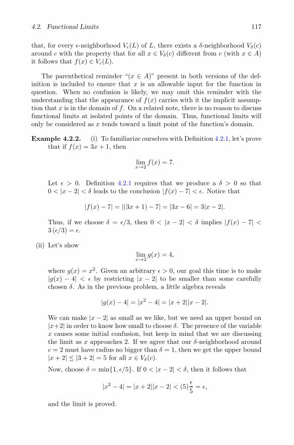
4.2. Functional Limits 117
that, for every ε-neighborhood Vε(L) of L, there exists a δ-neighborhood Vδ(c)around c with the property that for all x ∈ Vδ(c) different from c (with x ∈ A)it follows that f(x) ∈ Vε(L).
The parenthetical reminder “(x ∈ A)” present in both versions of the def-inition is included to ensure that x is an allowable input for the function inquestion. When no confusion is likely, we may omit this reminder with theunderstanding that the appearance of f(x) carries with it the implicit assump-tion that x is in the domain of f . On a related note, there is no reason to discussfunctional limits at isolated points of the domain. Thus, functional limits willonly be considered as x tends toward a limit point of the function’s domain.
Example 4.2.2. (i) To familiarize ourselves with Definition 4.2.1, let’s provethat if f(x) = 3x+ 1, then
limx→2
f(x) = 7.
Let ε > 0. Definition 4.2.1 requires that we produce a δ > 0 so that0 < |x− 2| < δ leads to the conclusion |f(x)− 7| < ε. Notice that
|f(x)− 7| = |(3x+ 1)− 7| = |3x− 6| = 3|x− 2|.
Thus, if we choose δ = ε/3, then 0 < |x − 2| < δ implies |f(x) − 7| <3 (ε/3) = ε.
(ii) Let’s show
limx→2
g(x) = 4,
where g(x) = x2. Given an arbitrary ε > 0, our goal this time is to make|g(x) − 4| < ε by restricting |x − 2| to be smaller than some carefullychosen δ. As in the previous problem, a little algebra reveals
|g(x)− 4| = |x2 − 4| = |x+ 2||x− 2|.
We can make |x− 2| as small as we like, but we need an upper bound on|x+2| in order to know how small to choose δ. The presence of the variablex causes some initial confusion, but keep in mind that we are discussingthe limit as x approaches 2. If we agree that our δ-neighborhood aroundc = 2 must have radius no bigger than δ = 1, then we get the upper bound|x+ 2| ≤ |3 + 2| = 5 for all x ∈ Vδ(c).
Now, choose δ = min{1, ε/5}. If 0 < |x− 2| < δ, then it follows that
|x2 − 4| = |x+ 2||x− 2| < (5)ε
5= ε,
and the limit is proved.

118 Chapter 4. Functional Limits and Continuity
Sequential Criterion for Functional Limits
We worked very hard in Chapter 2 to derive an impressive list of proper-ties enjoyed by sequential limits. In particular, the Algebraic Limit Theorem(Theorem 2.3.3) and the Order Limit Theorem (Theorem 2.3.4) proved invalu-able in a large number of the arguments that followed. Not surprisingly, weare going to need analogous statements for functional limits. Although it is notdifficult to generate independent proofs for these statements, all of them willfollow quite naturally from their sequential analogs once we derive the sequen-tial criterion for functional limits motivated in the opening discussion of thischapter.
Theorem 4.2.3 (Sequential Criterion for Functional Limits). Given afunction f : A → R and a limit point c of A, the following two statements areequivalent:
(i) limx→c
f(x) = L.
(ii) For all sequences (xn) ⊆ A satisfying xn �= c and (xn) → c, it follows thatf(xn) → L.
Proof. (⇒) Let’s first assume that limx→c f(x) = L. To prove (ii), we consideran arbitrary sequence (xn), which converges to c and satisfies xn �= c. Our goalis to show that the image sequence f(xn) converges to L. This is most easilyseen using the topological formulation of the definition.
Let ε > 0. Because we are assuming (i), Definition 4.2.1B implies thatthere exists Vδ(c) with the property that all x ∈ Vδ(c) different from c satisfyf(x) ∈ Vε(L). All we need to do then is argue that our particular sequence (xn)is eventually in Vδ(c). But we are assuming that (xn) → c. This implies thatthere exists a point xN after which xn ∈ Vδ(c). It follows that n ≥ N impliesf(xn) ∈ Vε(L), as desired.
(⇐) For this implication we give a contrapositive proof, which is essentiallya proof by contradiction. Thus, we assume that statement (ii) is true, andcarefully negate statement (i). To say that
limx→c
f(x) �= L
means that there exists at least one particular ε0 > 0 for which no δ is a suitableresponse. In other words, no matter what δ > 0 we try, there will always be atleast one point
x ∈ Vδ(c) with x �= c for which f(x) /∈ Vε0(L).
Now consider δn = 1/n. From the preceding discussion, it follows that for eachn ∈ N we may pick an xn ∈ Vδn(c) with xn �= c and f(xn) /∈ Vε0(L). But nownotice that the result of this is a sequence (xn) → c with xn �= c, where theimage sequence f(xn) certainly does not converge to L.
Because this contradicts (ii), which we are assuming is true for this argument,we may conclude that (i) must also hold.

4.2. Functional Limits 119
Theorem 4.2.3 has several useful corollaries. In addition to the previouslyadvertised benefit of granting us some short proofs of statements about howfunctional limits interact with algebraic combinations of functions, we also getan economical way of establishing that certain limits do not exist.
Corollary 4.2.4 (Algebraic Limit Theorem for Functional Limits). Letf and g be functions defined on a domain A ⊆ R, and assume limx→c f(x) = Land limx→c g(x) = M for some limit point c of A. Then,
(i) limx→c
kf(x) = kL for all k ∈ R,
(ii) limx→c
[f(x) + g(x)] = L+M ,
(iii) limx→c
[f(x)g(x)] = LM , and
(iv) limx→c
f(x)/g(x) = L/M , provided M �= 0.
Proof. These follow from Theorem 4.2.3 and the Algebraic Limit Theorem forsequences. The details are requested in Exercise 4.2.1.
Corollary 4.2.5 (Divergence Criterion for Functional Limits). Let f bea function defined on A, and let c be a limit point of A. If there exist twosequences (xn) and (yn) in A with xn �= c and yn �= c and
lim xn = lim yn = c but lim f(xn) �= lim f(yn),
then we can conclude that the functional limit limx→c f(x) does not exist.
Example 4.2.6. Assuming the familiar properties of the sine function, let’sshow that limx→0 sin(1/x) does not exist (Fig. 4.5).
If xn = 1/2nπ and yn = 1/(2nπ + π/2), then lim(xn) = lim(yn) = 0.However, sin(1/xn) = 0 for all n ∈ N while sin(1/yn) = 1. Thus,
lim sin(1/xn) �= lim sin(1/yn),
so by Corollary 4.2.5, limx→0 sin(1/x) does not exist.
Figure 4.5: The function sin(1/x) near zero.

120 Chapter 4. Functional Limits and Continuity
Exercises
Exercise 4.2.1. (a) Supply the details for how Corollary 4.2.4 part (ii) followsfrom the Sequential Criterion for Functional Limits in Theorem 4.2.3 andthe Algebraic Limit Theorem for sequences proved in Chapter 2.
(b) Now, write another proof of Corollary 4.2.4 part (ii) directly from Defini-tion 4.2.1 without using the sequential criterion in Theorem 4.2.3.
(c) Repeat (a) and (b) for Corollary 4.2.4 part (iii).
Exercise 4.2.2. For each stated limit, find the largest possible δ-neighborhoodthat is a proper response to the given ε challenge.
(a) limx→3(5x− 6) = 9, where ε = 1.
(b) limx→4√x = 2, where ε = 1.
(c) limx→π[[x]] = 3, where ε = 1. (The function [[x]] returns the greatestinteger less than or equal to x.)
(d) limx→π[[x]] = 3, where ε = .01.
Exercise 4.2.3. Review the definition of Thomae’s function t(x) fromSection 4.1.
(a) Construct three different sequences (xn), (yn), and (zn), each of whichconverges to 1 without using the number 1 as a term in the sequence.
(b) Now, compute lim t(xn), lim t(yn), and lim t(zn).
(c) Make an educated conjecture for limx→1 t(x), and use Definition 4.2.1B toverify the claim. (Given ε > 0, consider the set of points {x ∈ R : t(x) ≥ ε}.Argue that all the points in this set are isolated.)
Exercise 4.2.4. Consider the reasonable but erroneous claim that
limx→10
1/[[x]] = 1/10.
(a) Find the largest δ that represents a proper response to the challenge ofε = 1/2.
(b) Find the largest δ that represents a proper response to ε = 1/50.
(c) Find the largest ε challenge for which there is no suitable δ responsepossible.

4.2. Functional Limits 121
Exercise 4.2.5. Use Definition 4.2.1 to supply a proper proof for the followinglimit statements.
(a) limx→2(3x+ 4) = 10.
(b) limx→0 x3 = 0.
(c) limx→2(x2 + x− 1) = 5.
(d) limx→3 1/x = 1/3.
Exercise 4.2.6. Decide if the following claims are true or false, and give shortjustifications for each conclusion.
(a) If a particular δ has been constructed as a suitable response to a particularε challenge, then any smaller positive δ will also suffice.
(b) If limx→a f(x) = L and a happens to be in the domain of f , then L = f(a).
(c) If limx→a f(x) = L, then limx→a 3[f(x)− 2]2 = 3(L− 2)2.
(d) If limx→a f(x) = 0, then limx→a f(x)g(x) = 0 for any function g (withdomain equal to the domain of f .)
Exercise 4.2.7. Let g : A → R and assume that f is a bounded function on Ain the sense that there exists M > 0 satisfying |f(x)| ≤ M for all x ∈ A.
Show that if limx→c g(x) = 0, then limx→c g(x)f(x) = 0 as well.
Exercise 4.2.8. Compute each limit or state that it does not exist. Use thetools developed in this section to justify each conclusion.
(a) limx→2|x−2|x−2
(b) limx→7/4|x−2|x−2
(c) limx→0(−1)[[1/x]]
(d) limx→03√x(−1)[[1/x]]
Exercise 4.2.9 (Infinite Limits). The statement limx→0 1/x2 = ∞ certainly
makes intuitive sense. To construct a rigorous definition in the challenge–response style of Definition 4.2.1 for an infinite limit statement of this form,we replace the (arbitrarily small) ε > 0 challenge with an (arbitrarily large)M > 0 challenge:
Definition: limx→c f(x) = ∞ means that for all M > 0 we can find a δ > 0such that whenever 0 < |x− c| < δ, it follows that f(x) > M .
(a) Show limx→0 1/x2 = ∞ in the sense described in the previous definition.
(b) Now, construct a definition for the statement limx→∞ f(x) = L. Showlimx→∞ 1/x = 0.

122 Chapter 4. Functional Limits and Continuity
(c) What would a rigorous definition for limx→∞ f(x) = ∞ look like? Givean example of such a limit.
Exercise 4.2.10 (Right and Left Limits). Introductory calculus coursestypically refer to the right-hand limit of a function as the limit obtained by“letting x approach a from the right-hand side.”
(a) Give a proper definition in the style of Definition 4.2.1 for the right-handand left-hand limit statements:
limx→a+
f(x) = L and limx→a−
f(x) = M.
(b) Prove that limx→a f(x) = L if and only if both the right and left-handlimits equal L.
Exercise 4.2.11 (Squeeze Theorem). Let f, g, and h satisfy f(x) ≤ g(x) ≤h(x) for all x in some common domain A. If limx→c f(x) = L and limx→c h(x) =L at some limit point c of A, show limx→c g(x) = L as well.
4.3 Continuous Functions
We now come to a significant milestone in our progress toward a rigorous theoryof real-valued functions—a proper definition of the seminal concept of continuitythat avoids any intuitive appeals to “unbroken curves” or functions without“jumps” or “holes.”
Definition 4.3.1 (Continuity). A function f : A → R is continuous at apoint c ∈ A if, for all ε > 0, there exists a δ > 0 such that whenever |x− c| < δ(and x ∈ A) it follows that |f(x)− f(c)| < ε.
If f is continuous at every point in the domain A, then we say that f iscontinuous on A.
The definition of continuity looks much like the definition for functionallimits, with a few subtle differences. The most important is that we require thepoint c to be in the domain of f . The value f(c) then becomes the value oflimx→c f(x). With this observation in mind, it is tempting to shorten Defini-tion 4.3.1 to say that f is continuous at c ∈ A if
limx→c
f(x) = f(c).
This is fine as long as c is a limit point of A. If c is an isolated point of A,then limx→c f(x) isn’t defined but Definition 4.3.1 can still be applied. An un-remarkable but noteworthy consequence of this definition is that functions arecontinuous at isolated points of their domains (Exercise 4.3.5).
We saw in the previous section that, in addition to the standard ε–δ definition,functional limits have a useful formulation in terms of sequences. The same istrue of continuity. The next theorem summarizes these various equivalent waysto characterize the continuity of a function at a given point.
4.3. Continuous Functions 123
Theorem 4.3.2 (Characterizations of Continuity). Let f : A → R, and letc ∈ A. The function f is continuous at c if and only if any one of the followingthree conditions is met:
(i) For all ε > 0, there exists a δ > 0 such that |x−c| < δ (and x ∈ A) implies|f(x)− f(c)| < ε;
(ii) For all Vε(f(c)), there exists a Vδ(c) with the property that x ∈ Vδ(c) (andx ∈ A) implies f(x) ∈ Vε(f(c));
(iii) For all (xn) → c (with xn ∈ A), it follows that f(xn) → f(c).
If c is a limit point of A, then the above conditions are equivalent to
(iv) limx→c
f(x) = f(c).
Proof. Statement (i) is just Definition 4.3.1, and statement (ii) is the standardrewording of (i) using topological neighborhoods in place of the absolute valuenotation. Statement (iii) is equivalent to (i) via an argument nearly identical tothat of Theorem 4.2.3, with some slight modifications for when xn = c. Finally,statement (iv) is seen to be equivalent to (i) by considering Definition 4.2.1 andobserving that the case x = c (which is excluded in the definition of functionallimits) leads to the requirement f(c) ∈ Vε(f(c)), which is trivially true.
The length of this list is somewhat deceiving. Statements (i), (ii), and (iv)are closely related and essentially remind us that functional limits have an ε–δformulation as well as a topological description. Statement (iii), however, isqualitatively different from the others. As a general rule, the sequential char-acterization of continuity is typically the most useful for demonstrating that afunction is not continuous at some point.
Corollary 4.3.3 (Criterion for Discontinuity). Let f : A → R, and letc ∈ A be a limit point of A. If there exists a sequence (xn) ⊆ A where (xn) → cbut such that f(xn) does not converge to f(c), we may conclude that f is notcontinuous at c.
The sequential characterization of continuity is also important for the otherreasons that it was important for functional limits. In particular, it allowsus to bring our catalog of results about the behavior of sequences to bear onthe study of continuous functions. The next theorem should be compared toCorollary 4.2.3 as well as to Theorem 2.3.3.
Theorem 4.3.4 (Algebraic Continuity Theorem). Assume f : A → R andg : A → R are continuous at a point c ∈ A. Then,
(i) kf(x) is continuous at c for all k ∈ R;
(ii) f(x) + g(x) is continuous at c;
(iii) f(x)g(x) is continuous at c; and
(iv) f(x)/g(x) is continuous at c, provided the quotient is defined.

124 Chapter 4. Functional Limits and Continuity
Figure 4.6: The function x sin(1/x) near zero.
Proof. All of these statements can be quickly derived from Corollary 4.2.4 andTheorem 4.3.2.
These results provide us with the tools we need to firm up our argumentsin the opening section of this chapter about the behavior of Dirichlet’s functionand Thomae’s function. The details are requested in Exercise 4.3.7. Here aresome more examples of arguments for and against continuity of some familiarfunctions.
Example 4.3.5. All polynomials are continuous on R. In fact, rational func-tions (i.e., quotients of polynomials) are continuous wherever they are defined.
To see why this is so, consider the identity function g(x) = x. Because|g(x) − g(c)| = |x − c|, we can respond to a given ε > 0 by choosing δ = ε,and it follows that g is continuous on all of R. It is even simpler to show thata constant function f(x) = k, is continuous. (Letting δ = 1 regardless of thevalue of ε does the trick.) Because an arbitrary polynomial
p(x) = a0 + a1x+ a2x2 + · · ·+ anx
n
consists of sums and products of g(x) with different constant functions, we mayconclude from Theorem 4.3.4 that p(x) is continuous.
Likewise, Theorem 4.3.4 implies that quotients of polynomials are continuousas long as the denominator is not zero.
Example 4.3.6. In Example 4.2.6, we saw that the oscillations of sin(1/x) areso rapid near the origin that limx→0 sin(1/x) does not exist. Now, consider thefunction
g(x) =
{x sin(1/x) if x �= 00 if x = 0.
To investigate the continuity of g at c = 0 (Fig. 4.6), we can estimate
|g(x)− g(0)| = |x sin(1/x)− 0| ≤ |x|.

4.3. Continuous Functions 125
Given ε > 0, set δ = ε, so that whenever |x − 0| = |x| < δ it follows that|g(x)− g(0)| < ε. Thus, g is continuous at the origin.
Example 4.3.7. Throughout the exercises we have been using the greatestinteger function h(x) = [[x]] which for each x ∈ R returns the largest integern ∈ Z satisfying n ≤ x. This familiar step function certainly has discontinuous“jumps” at each integer value of its domain, but it is a useful exercise to tryand articulate this observation in the language of analysis.
Given m ∈ Z, define the sequence (xn) by xn = m − 1/n. It follows that(xn) → m, but
h(xn) → (m− 1),
which does not equal m = h(m). By Corollary 4.3.3, we see that h fails to becontinuous at each m ∈ Z.
Now let’s see why h is continuous at a point c /∈ Z. Given ε > 0, we must finda δ-neighborhood Vδ(c) such that x ∈ Vδ(c) implies h(x) ∈ Vε(h(c)). We knowthat c ∈ R falls between consecutive integers n < c < n + 1 for some n ∈ Z.If we take δ = min{c − n, (n + 1)− c}, then it follows from the definition of hthat h(x) = h(c) for all x ∈ Vδ(c). Thus, we certainly have
h(x) ∈ Vε(h(c))
whenever x ∈ Vδ(c).
This latter proof is quite different from the typical situation in that the valueof δ does not actually depend on the choice of ε. Usually, a smaller ε requires asmaller δ in response, but here the same value of δ works no matter how smallε is chosen.
Example 4.3.8. Consider f(x) =√x defined on A = {x ∈ R : x ≥ 0}.
Exercise 2.3.1 outlines a sequential proof that f is continuous on A. Here, wegive an ε–δ proof of the same fact.
Let ε > 0. We need to argue that |f(x) − f(c)| can be made less than ε forall values of x in some δ neighborhood around c. If c = 0, this reduces to thestatement
√x < ε, which happens as long as x < ε2. Thus, if we choose δ = ε2,
we see that |x− 0| < δ implies |f(x)− 0| < ε.
For a point c ∈ A different from zero, we need to estimate |√x−√c|. This
time, write
|√x−√c| = |√x−√
c|(√
x+√c√
x+√c
)
=|x− c|√x+
√c≤ |x− c|√
c.
In order to make this quantity less than ε, it suffices to pick δ = ε√c. Then,
|x− c| < δ implies
|√x−√c| < ε
√c√c
= ε,
as desired.

126 Chapter 4. Functional Limits and Continuity
Although we have now shown that both polynomials and the square rootfunction are continuous, the Algebraic Continuity Theorem does not providethe justification needed to conclude that a function such as h(x) =
√3x2 + 5 is
continuous. For this, we must prove that compositions of continuous functionsare continuous.
Theorem 4.3.9 (Composition of Continuous Functions). Given f : A→Rand g : B → R, assume that the range f(A) = {f(x) : x ∈ A} is contained inthe domain B so that the composition g ◦ f(x) = g(f(x)) is defined on A.
If f is continuous at c ∈ A, and if g is continuous at f(c) ∈ B, then g ◦ f iscontinuous at c.
Proof. Exercise 4.3.3.
Exercises
Exercise 4.3.1. Let g(x) = 3√x.
(a) Prove that g is continuous at c = 0.
(b) Prove that g is continuous at a point c �= 0. (The identity a3 − b3 =(a− b)(a2 + ab+ b2) will be helpful.)
Exercise 4.3.2. To gain a deeper understanding of the relationship betweenε and δ in the definition of continuity, let’s explore some modest variations ofDefinition 4.3.1. In all of these, let f be a function defined on all of R.
(a) Let’s say f is onetinuous at c if for all ε > 0 we can choose δ = 1 and itfollows that |f(x)− f(c)| < ε whenever |x− c| < δ. Find an example of afunction that is onetinuous on all of R.
(b) Let’s say f is equaltinuous at c if for all ε > 0 we can choose δ = ε and itfollows that |f(x)− f(c)| < ε whenever |x− c| < δ. Find an example of afunction that is equaltinuous on R that is nowhere onetinuous, or explainwhy there is no such function.
(c) Let’s say f is lesstinuous at c if for all ε > 0 we can choose 0 < δ < ε andit follows that |f(x)−f(c)| < ε whenever |x−c| < δ. Find an example of afunction that is lesstinuous on R that is nowhere equaltinuous, or explainwhy there is no such function.
(d) Is every lesstinuous function continuous? Is every continuous functionlesstinuous? Explain.
Exercise 4.3.3. (a) Supply a proof for Theorem 4.3.9 using the ε–δ charac-terization of continuity.
(b) Give another proof of this theorem using the sequential characterizationof continuity (from Theorem 4.3.2 (iii)).

4.3. Continuous Functions 127
Exercise 4.3.4. Assume f and g are defined on all of R and that limx→p
f(x) = q
and limx→q
g(x) = r.
(a) Give an example to show that it may not be true that
limx→p
g(f(x)) = r.
(b) Show that the result in (a) does follow if we assume f and g are continuous.
(c) Does the result in (a) hold if we only assume f is continuous? How aboutif we only assume that g is continuous?
Exercise 4.3.5. Show using Definition 4.3.1 that if c is an isolated point ofA ⊆ R, then f : A → R is continuous at c.
Exercise 4.3.6. Provide an example of each or explain why the request isimpossible.
(a) Two functions f and g, neither of which is continuous at 0 but such thatf(x)g(x) and f(x) + g(x) are continuous at 0.
(b) A function f(x) continuous at 0 and g(x) not continuous at 0 such thatf(x) + g(x) is continuous at 0.
(c) A function f(x) continuous at 0 and g(x) not continuous at 0 such thatf(x)g(x) is continuous at 0.
(d) A function f(x) not continuous at 0 such that f(x) + 1f(x) is continuous
at 0.
(e) A function f(x) not continuous at 0 such that [f(x)]3 is continuous at 0.
Exercise 4.3.7. (a) Referring to the proper theorems, give a formal argu-ment that Dirichlet’s function from Section 4.1 is nowhere-continuouson R.
(b) Review the definition of Thomae’s function in Section 4.1 and demonstratethat it fails to be continuous at every rational point.
(c) Use the characterization of continuity in Theorem 4.3.2 (iii) to show thatThomae’s function is continuous at every irrational point in R. (Givenε > 0, consider the set of points {x ∈ R : t(x) ≥ ε}.)
Exercise 4.3.8. Decide if the following claims are true or false, providing eithera short proof or counterexample to justify each conclusion. Assume throughoutthat g is defined and continuous on all of R.
(a) If g(x) ≥ 0 for all x < 1, then g(1) ≥ 0 as well.
(b) If g(r) = 0 for all r ∈ Q, then g(x) = 0 for all x ∈ R.

128 Chapter 4. Functional Limits and Continuity
(c) If g(x0) > 0 for a single point x0 ∈ R, then g(x) is in fact strictly positivefor uncountably many points.
Exercise 4.3.9. Assume h : R → R is continuous on R and let K = {x :h(x) = 0}. Show that K is a closed set.
Exercise 4.3.10. Observe that if a and b are real numbers, then
max{a, b} =1
2[(a+ b) + |a− b|].
(a) Show that if f1, f2, . . . , fn are continuous functions, then
g(x) = max{f1(x), f2(x), . . . , fn(x)}is a continuous function.
(b) Let’s explore whether the result in (a) extends to the infinite case. Foreach n ∈ N, define fn on R by
fn(x) =
{1 if |x| ≥ 1/nn|x| if |x| < 1/n.
Now explicitly compute h(x) = sup{f1(x), f2(x), f3(x), . . .}.Exercise 4.3.11 (Contraction Mapping Theorem). Let f be a functiondefined on all of R, and assume there is a constant c such that 0 < c < 1 and
|f(x)− f(y)| ≤ c|x− y|for all x, y ∈ R.
(a) Show that f is continuous on R.
(b) Pick some point y1 ∈ R and construct the sequence
(y1, f(y1), f(f(y1)), . . .).
In general, if yn+1 = f(yn), show that the resulting sequence (yn) is aCauchy sequence. Hence we may let y = lim yn.
(c) Prove that y is a fixed point of f (i.e., f(y) = y) and that it is unique inthis regard.
(d) Finally, prove that if x is any arbitrary point in R, then the sequence(x, f(x), f(f(x)), . . .) converges to y defined in (b).
Exercise 4.3.12. Let F ⊆ R be a nonempty closed set and define g(x) =inf{|x − a| : a ∈ F}. Show that g is continuous on all of R and g(x) �= 0 forall x /∈ F .
Exercise 4.3.13. Let f be a function defined on all of R that satisfies theadditive condition f(x+ y) = f(x) + f(y) for all x, y ∈ R.

4.4. Continuous Functions on Compact Sets 129
(a) Show that f(0) = 0 and that f(−x) = −f(x) for all x ∈ R.
(b) Let k = f(1). Show that f(n) = kn for all n ∈ N, and then prove thatf(z) = kz for all z ∈ Z. Now, prove that f(r) = kr for any rationalnumber r.
(c) Show that if f is continuous at x = 0, then f is continuous at every pointin R and conclude that f(x) = kx for all x ∈ R. Thus, any additivefunction that is continuous at x = 0 must necessarily be a linear functionthrough the origin.
Exercise 4.3.14. (a) Let F be a closed set. Construct a function f : R → Rsuch that the set of points where f fails to be continuous is precisely F .(The concept of the interior of a set, discussed in Exercise 3.2.14, may beuseful.)
(b) Now consider an open set O. Construct a function g : R → R whose setof discontinuous points is precisely O. (For this problem, the function inExercise 4.3.12 may be useful.)
4.4 Continuous Functions on Compact Sets
Given a function f : A → R and a subset B ⊆ A, the notation f(B) refers tothe range of f over the set B; that is,
f(B) = {f(x) : x ∈ B}.The adjectives open, closed, bounded, compact, perfect, and connected are
all used to describe subsets of the real line. An interesting question is to sortout which, if any, of these properties are preserved when a particular set B ismapped to f(B) via a continuous function. For instance, if B is open and fis continuous, is f(B) necessarily open? The answer to this question is no. Iff(x) = x2 and B is the open interval (−1, 1), then f(B) is the interval [0, 1),which is not open.
The corresponding conjecture for closed sets also turns out to be false, al-though constructing a counterexample requires a little more thought. Considerthe function
g(x) =1
1 + x2
and the closed set B = [0,∞) = {x : x ≥ 0}. Because g(B) = (0, 1] is notclosed, we must conclude that continuous functions do not, in general, mapclosed sets to closed sets. Notice, however, that our particular counterexamplerequired using an unbounded closed set B. This is not incidental. Sets that areclosed and bounded—that is, compact sets—always get mapped to closed andbounded subsets by continuous functions.
Theorem 4.4.1 (Preservation of Compact Sets). Let f : A → R be con-tinuous on A. If K ⊆ A is compact, then f(K) is compact as well.

130 Chapter 4. Functional Limits and Continuity
Proof. Let (yn) be an arbitrary sequence contained in the range set f(K).To prove this result, we must find a subsequence (ynk
), which converges toa limit also in f(K). The strategy is to take advantage of the assumption thatthe domain set K is compact by translating the sequence (yn)—which is in therange of f—back to a sequence in the domain K.
To assert that (yn) ⊆ f(K) means that, for each n ∈ N, we can find (at leastone) xn ∈ K with f(xn) = yn. This yields a sequence (xn) ⊆ K. Because K iscompact, there exists a convergent subsequence (xnk
) whose limit x = limxnk
is also in K. Finally, we make use of the fact that f is assumed to be continuouson A and so is continuous at x in particular. Given that (xnk
) → x, we concludethat (ynk
) → f(x). Because x ∈ K, we have that f(x) ∈ f(K), and hence f(K)is compact.
An extremely important corollary is obtained by combining this result withthe observation that compact sets are bounded and contain their supremumsand infimums.
Theorem 4.4.2 (Extreme Value Theorem). If f : K → R is continuous ona compact set K ⊆ R, then f attains a maximum and minimum value. In otherwords, there exist x0, x1 ∈ K such that f(x0) ≤ f(x) ≤ f(x1) for all x ∈ K.
Proof. Because f(K) is compact, we can set α = sup f(K) and know α ∈ f(K)(Exercise 3.3.1). It follows that there exist x1 ∈ K with α = f(x1). Theargument for the minimum value is similar.
Uniform Continuity
Although we have proved that polynomials are always continuous on R, thereis an important lesson to be learned by constructing direct proofs that thefunctions f(x) = 3x + 1 and g(x) = x2 (previously studied in Example 4.2.2)are everywhere continuous.
Example 4.4.3. (i) To show directly that f(x) = 3x + 1 is continuous atan arbitrary point c ∈ R, we must argue that |f(x) − f(c)| can be madearbitrarily small for values of x near c. Now,
|f(x)− f(c)| = |(3x+ 1)− (3c+ 1)| = 3|x− c|,so, given ε > 0, we choose δ = ε/3. Then, |x− c| < δ implies
|f(x) − f(c)| = 3|x− c| < 3( ε
3
)= ε.
Of particular importance for this discussion is the fact that the choice ofδ is the same regardless of which point c ∈ R we are considering.
(ii) Let’s contrast this with what happens when we prove g(x) = x2 is contin-uous on R. Given c ∈ R, we have
|g(x)− g(c)| = |x2 − c2| = |x− c||x+ c|.

4.4. Continuous Functions on Compact Sets 131
As discussed in Example 4.2.2, we need an upper bound on |x+ c|, whichis obtained by insisting that our choice of δ not exceed 1. This guaranteesthat all values of x under consideration will necessarily fall in the interval(c− 1, c+ 1). It follows that
|x+ c| ≤ |x|+ |c| ≤ (|c|+ 1) + |c| = 2|c|+ 1.
Now, let ε > 0. If we choose δ = min{1, ε/(2|c| + 1)}, then |x − c| < δimplies
|f(x)− f(c)| = |x− c||x+ c| <(
ε
2|c|+ 1
)
(2|c|+ 1) = ε.
Now, there is nothing deficient about this argument, but it is importantto notice that, in the second proof, the algorithm for choosing the response δdepends on the value of c. The statement
δ =ε
2|c|+ 1
means that larger values of c are going to require smaller values of δ, a factthat should be evident from a consideration of the graph of g(x) = x2 (Fig. 4.7).Given, say, ε = 1, a response of δ = 1/3 is sufficient for c = 1 because 2/3 <x < 4/3 certainly implies 0 < x2 < 2. However, if c = 10, then the steepnessof the graph of g(x) means that a much smaller δ is required—δ = 1/21 by ourrule—to force 99 < x2 < 101.
The next definition is meant to distinguish between these two examples.
�
�
�
�
�
�
Vε(f(c1))
{
Vε(f(c2))
{
Vε(f(c3))
{
c1
Vδ1 (c1)
c2
Vδ2 (c2)
c3
Vδ3 (c3)
Figure 4.7: g(x) = x2; A larger c requires a smaller δ.

132 Chapter 4. Functional Limits and Continuity
Definition 4.4.4 (Uniform Continuity). A function f : A → R is uniformlycontinuous on A if for every ε > 0 there exists a δ > 0 such that for all x, y ∈ A,|x− y| < δ implies |f(x)− f(y)| < ε.
Recall that to say that “f is continuous on A” means that f is continuous ateach individual point c ∈ A. In other words, given ε > 0 and c ∈ A, we can finda δ > 0 perhaps depending on c such that if |x− c| < δ, then |f(x)− f(c)| < ε.Uniform continuity is a strictly stronger property. The key distinction betweenasserting that f is “uniformly continuous on A” versus simply “continuous on A”is that, given an ε > 0, a single δ > 0 can be chosen that works simultaneouslyfor all points c in A. To say that a function is not uniformly continuous on a setA, then, does not necessarily mean it is not continuous at some point. Rather, itmeans that there is some ε0 > 0 for which no single δ > 0 is a suitable responsefor all c ∈ A.
Theorem 4.4.5 (Sequential Criterion for Absence of Uniform Conti-nuity). A function f : A → R fails to be uniformly continuous on A if andonly if there exists a particular ε0 > 0 and two sequences (xn) and (yn) in Asatisfying
|xn − yn| → 0 but |f(xn)− f(yn)| ≥ ε0.
Proof. The negation of Definition 4.4.4 states that f is not uniformly continuouson A if and only if there exists ε0 > 0 such that for all δ > 0 we can find twopoints x and y satisfying |x − y| < δ but with |f(x) − f(y)| ≥ ε0. Thus, ifwe set δ1 = 1, then there exist two points x1 and y1 where |x1 − y1| < 1 but|f(x1)− f(y1)| ≥ ε0.
In a similar way, if we set δn = 1/n where n ∈ N, it follows that thereexist points xn and yn with |xn − yn| < 1/n but where |f(xn) − f(yn)| ≥ ε0.The resulting sequences (xn) and (yn) satisfy the requirements described in thetheorem.
Conversely, if ε0, (xn) and (yn) exist as described, it is straightforward tosee that no δ > 0 is a suitable response for ε0.
Example 4.4.6. The function h(x) = sin(1/x) (Fig. 4.5) is continuous at everypoint in the open interval (0, 1) but is not uniformly continuous on this interval.The problem arises near zero, where the increasingly rapid oscillations takedomain values that are quite close together to range values a distance 2 apart.To illustrate Theorem 4.4.5, take ε0 = 2 and set
xn =1
π/2 + 2nπand yn =
1
3π/2 + 2nπ.
Because each of these sequences tends to zero, we have |xn − yn| → 0, and ashort calculation reveals |h(xn)− h(yn)| = 2 for all n ∈ N.
Whereas continuity is defined at a single point, uniform continuity is alwaysdiscussed in reference to a particular domain. In Example 4.4.3, we were notable to prove that g(x) = x2 is uniformly continuous on R because larger
4.4. Continuous Functions on Compact Sets 133
values of x require smaller and smaller values of δ. (As another illustrationof Theorem 4.4.5, take xn = n and yn = n + 1/n.) It is true, however, thatg(x) is uniformly continuous on the bounded set [−10, 10]. Returning to theargument set forth in Example 4.4.3 (ii), notice that if we restrict our attentionto the domain [−10, 10], then |x+ y| ≤ 20 for all x and y. Given ε > 0, we cannow choose δ = ε/20, and verify that if x, y ∈ [−10, 10] satisfy |x− y| < δ, then
|f(x)− f(y)| = |x2 − y2| = |x− y||x+ y| <( ε
20
)20 = ε.
In fact, it is not difficult to see how to modify this argument to show that g(x)is uniformly continuous on any bounded set A in R.
Now, Example 4.4.6 is included to keep us from jumping to the erroneousconclusion that functions that are continuous on bounded domains are neces-sarily uniformly continuous. A general result does follow, however, if we assumethat the domain is compact.
Theorem 4.4.7 (Uniform Continuity on Compact Sets). A function thatis continuous on a compact set K is uniformly continuous on K.
Proof. Assume f : K → R is continuous at every point of a compact setK ⊆ R.To prove that f is uniformly continuous on K we argue by contradiction.
By the criterion in Theorem 4.4.5, if f is not uniformly continuous on K,then there exist two sequences (xn) and (yn) in K such that
lim |xn − yn| = 0 while |f(xn)− f(yn)| ≥ ε0
for some particular ε0 > 0. Because K is compact, the sequence (xn) has aconvergent subsequence (xnk
) with x = limxnkalso in K.
We could use the compactness of K again to produce a convergent subse-quence of (yn), but notice what happens when we consider the particular sub-sequence (ynk
) consisting of those terms in (yn) that correspond to the termsin the convergent subsequence (xnk
). By the Algebraic Limit Theorem,
lim(ynk) = lim((ynk
− xnk) + xnk
) = 0 + x.
The conclusion is that both (xnk) and (ynk
) converge to x ∈ K. Because f isassumed to be continuous at x, we have lim f(xnk
) = f(x) and lim f(ynk) =
f(x), which implies
lim(f(xnk)− f(ynk
)) = 0.
A contradiction arises when we recall that (xn) and (yn) were chosen to satisfy
|f(xn)− f(yn)| ≥ ε0
for all n ∈ N. We conclude, then, that f is indeed uniformly continuous on K.

134 Chapter 4. Functional Limits and Continuity
Exercises
Exercise 4.4.1. (a) Show that f(x) = x3 is continuous on all of R.
(b) Argue, using Theorem 4.4.5, that f is not uniformly continuous on R.
(c) Show that f is uniformly continuous on any bounded subset of R.
Exercise 4.4.2. (a) Is f(x) = 1/x uniformly continuous on (0, 1)?
(b) Is g(x) =√x2 + 1 uniformly continuous on (0, 1)?
(c) Is h(x) = x sin(1/x) uniformly continuous on (0, 1)?
Exercise 4.4.3. Show that f(x) = 1/x2 is uniformly continuous on the set[1,∞) but not on the set (0, 1].
Exercise 4.4.4. Decide whether each of the following statements is true orfalse, justifying each conclusion.
(a) If f is continuous on [a, b] with f(x) > 0 for all a ≤ x ≤ b, then 1/f isbounded on [a, b] (meaning 1/f has bounded range).
(b) If f is uniformly continuous on a bounded set A, then f(A) is bounded.
(c) If f is defined on R and f(K) is compact whenever K is compact, then fis continuous on R.
Exercise 4.4.5. Assume that g is defined on an open interval (a, c) and it isknown to be uniformly continuous on (a, b] and [b, c), where a < b < c. Provethat g is uniformly continuous on (a, c).
Exercise 4.4.6. Give an example of each of the following, or state that such arequest is impossible. For any that are impossible, supply a short explanationfor why this is the case.
(a) A continuous function f : (0, 1) → R and a Cauchy sequence (xn) suchthat f(xn) is not a Cauchy sequence;
(b) A uniformly continuous function f : (0, 1) → R and a Cauchy sequence(xn) such that f(xn) is not a Cauchy sequence;
(c) A continuous function f : [0,∞) → R and a Cauchy sequence (xn) suchthat f(xn) is not a Cauchy sequence;
Exercise 4.4.7. Prove that f(x) =√x is uniformly continuous on [0,∞).
Exercise 4.4.8. Give an example of each of the following, or provide a shortargument for why the request is impossible.
(a) A continuous function defined on [0, 1] with range (0, 1).
(b) A continuous function defined on (0, 1) with range [0, 1].

4.4. Continuous Functions on Compact Sets 135
(c) A continuous function defined on (0, 1] with range (0, 1).
Exercise 4.4.9 (Lipschitz Functions). A function f : A → R is calledLipschitz if there exists a bound M > 0 such that
∣∣∣∣f(x)− f(y)
x− y
∣∣∣∣ ≤ M
for all x �= y ∈ A. Geometrically speaking, a function f is Lipschitz if there is auniform bound on the magnitude of the slopes of lines drawn through any twopoints on the graph of f .
(a) Show that if f : A → R is Lipschitz, then it is uniformly continuous on A.
(b) Is the converse statement true? Are all uniformly continuous functionsnecessarily Lipschitz?
Exercise 4.4.10. Assume that f and g are uniformly continuous functionsdefined on a common domain A. Which of the following combinations arenecessarily uniformly continuous on A:
f(x) + g(x), f(x)g(x),f(x)
g(x), f(g(x)) ?
(Assume that the quotient and the composition are properly defined and thusat least continuous.)
Exercise 4.4.11 (Topological Characterization of Continuity). Let g bedefined on all of R. If B is a subset of R, define the set g−1(B) by
g−1(B) = {x ∈ R : g(x) ∈ B}.
Show that g is continuous if and only if g−1(O) is open whenever O ⊆ R is anopen set.
Exercise 4.4.12. Review Exercise 4.4.11, and then determine which of thefollowing statements is true about a continuous function defined on R:
(a) f−1(B) is finite whenever B is finite.
(b) f−1(K) is compact whenever K is compact.
(c) f−1(A) is bounded whenever A is bounded.
(d) f−1(F ) is closed whenever F is closed.
Exercise 4.4.13 (Continuous Extension Theorem). (a) Show that auniformly continuous function preserves Cauchy sequences; that is, iff : A → R is uniformly continuous and (xn) ⊆ A is a Cauchy sequence,then show f(xn) is a Cauchy sequence.

136 Chapter 4. Functional Limits and Continuity
(b) Let g be a continuous function on the open interval (a, b). Prove thatg is uniformly continuous on (a, b) if and only if it is possible to definevalues g(a) and g(b) at the endpoints so that the extended function g iscontinuous on [a, b]. (In the forward direction, first produce candidatesfor g(a) and g(b), and then show the extended g is continuous.)
Exercise 4.4.14. Construct an alternate proof of Theorem 4.4.7 using theopen cover characterization of compactness from the Heine–Borel Theorem(Theorem 3.3.8 (iii)).
4.5 The Intermediate Value Theorem
The Intermediate Value Theorem (IVT) is the name given to the very intuitiveobservation that a continuous function f on a closed interval [a, b] attains everyvalue that falls between the range values f(a) and f(b) (Fig. 4.8).
Here is this observation in the language of analysis.
Theorem 4.5.1 (Intermediate Value Theorem). Let f : [a, b] → R becontinuous. If L is a real number satisfying f(a) < L < f(b) or f(a) > L >f(b), then there exists a point c ∈ (a, b) where f(c) = L.
This theorem was freely used by mathematicians of the 18th century (includ-ing Euler and Gauss) without any consideration of its validity. In fact, the firstanalytical proof was not offered until 1817 by Bolzano in a paper that also con-tains the first appearance of a somewhat modern definition of continuity. Thisemphasizes the significance of this result. As discussed in Section 4.1, Bolzanoand his contemporaries had arrived at a point in the evolution of mathematicswhere it was becoming increasingly important to firm up the foundations of thesubject. Doing so, however, was not simply a matter of going back and sup-plying the missing proofs. The real battle lay in first obtaining a thorough andmutually agreed-upon understanding of the relevant concepts. The importanceof the Intermediate Value Theorem for us is similar in that our understandingof continuity and the nature of the real line is now mature enough for a proof tobe possible. Indeed, there are several satisfying arguments for this simple result,each one isolating, in a slightly different way, the interplay between continuityand completeness.
Preservation of Connected Sets
The most potentially useful way to understand the Intermediate Value Theorem(IVT) is as a special case of the fact that continuous functions map connectedsets to connected sets. In Theorem 4.4.1, we saw that if f is a continuousfunction on a compact set K, then the range set f(K) is also compact. Theanalogous observation holds for connected sets.
Theorem 4.5.2 (Preservation of Connected Sets). Let f : G → R becontinuous. If E ⊆ G is connected, then f(E) is connected as well.

4.5. The Intermediate Value Theorem 137
a c b
f(a)
L
f(b)
Figure 4.8: Intermediate Value Theorem.
Proof. Intending to use the characterization of connected sets in Theorem 3.4.6,let f(E) = A ∪ B where A and B are disjoint and nonempty. Our goal is toproduce a sequence contained in one of these sets that converges to a limit inthe other.
Let
C = {x ∈ E : f(x) ∈ A} and D = {x ∈ E : f(x) ∈ B}.
The sets C and D are called the preimages of A and B, respectively. Using theproperties of A and B, it is straightforward to check that C and D are nonemptyand disjoint and satisfy E = C ∪ D. Now, we are assuming E is a connectedset, so by Theorem 3.4.6, there exists a sequence (xn) contained in one of C orD with x = lim xn contained in the other. Finally, because f is continuous at x,we get f(x) = lim f(xn). Thus, it follows that f(xn) is a convergent sequencecontained in either A or B while the limit f(x) is an element of the other. Withanother nod to Theorem 3.4.6, the proof is complete.
In R, a set is connected if and only if it is a (possibly unbounded) interval.This fact, together with Theorem 4.5.2, leads to a short proof of the Interme-diate Value Theorem (Exercise 4.5.1). We should point out that the proof ofTheorem 4.5.2 does not make use of the equivalence between connected sets andintervals in R but relies only on the general definitions. The previous commentthat this is the most useful way to approach IVT stems from the fact that,although it is not discussed here, the definitions of continuity and connected-ness can be easily adapted to higher-dimensional settings. Theorem 4.5.2, then,remains a valid conclusion in higher dimensions, whereas the Intermediate ValueTheorem is essentially a one-dimensional result.

138 Chapter 4. Functional Limits and Continuity
Completeness
A typical way the Intermediate Value Theorem is applied is to prove the exis-tence of roots. Given f(x) = x2 − 2, for instance, we see that f(1) = −1 andf(2) = 2. Therefore, there exists a point c ∈ (1, 2) where f(c) = 0.
In this case, we can easily compute c =√2, meaning that we really did not
need IVT to show that f has a root. We spent a good deal of time in Chapter 1proving that
√2 exists, which was only possible once we insisted on the Axiom of
Completeness as part of our assumptions about the real numbers. The fact thatthe Intermediate Value Theorem has just asserted that
√2 exists suggests that
another way to understand this result is in terms of the relationship betweenthe continuity of f and the completeness of R.
The Axiom of Completeness (AoC) from the first chapter states that“Nonempty sets that are bounded above have least upper bounds.” Later, wesaw that the Nested Interval Property (NIP) is an equivalent way to assert thatthe real numbers have no “gaps.” Either of these characterizations of complete-ness can be used as the cornerstone for an alternate proof of Theorem 4.5.1.
Proof. I. (First approach using AoC.) To simplify matters a bit, let’s considerthe special case where f is a continuous function satisfying f(a) < 0 < f(b) andshow that f(c) = 0 for some c ∈ (a, b). First let
K = {x ∈ [a, b] : f(x) ≤ 0}.
•a
K
b
f(a)
f(b)
�
c=supK
���
���
Notice that K is bounded above by b, and a ∈ K so K is not empty. Thus wemay appeal to the Axiom of Completeness to assert that c = supK exists.
There are three cases to consider:
f(c) > 0, f(c) < 0, and f(c) = 0.
The fact that c is the least upper bound of K can be used to rule out the firsttwo cases, resulting in the desired conclusion that f(c) = 0. The details arerequested in Exercise 4.5.5(a).
II. (Second approach using NIP.) Again, consider the special case whereL = 0 and f(a) < 0 < f(b). Let I0 = [a, b], and consider the midpoint
z = (a+ b)/2.
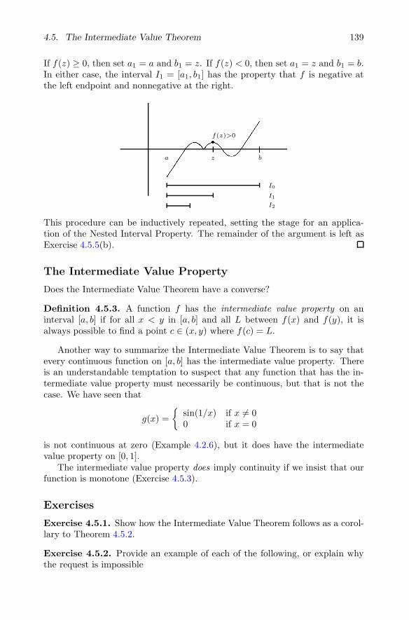
4.5. The Intermediate Value Theorem 139
If f(z) ≥ 0, then set a1 = a and b1 = z. If f(z) < 0, then set a1 = z and b1 = b.In either case, the interval I1 = [a1, b1] has the property that f is negative atthe left endpoint and nonnegative at the right.
•
a z b
f(z)>0
I0
I1
I2
This procedure can be inductively repeated, setting the stage for an applica-tion of the Nested Interval Property. The remainder of the argument is left asExercise 4.5.5(b).
The Intermediate Value Property
Does the Intermediate Value Theorem have a converse?
Definition 4.5.3. A function f has the intermediate value property on aninterval [a, b] if for all x < y in [a, b] and all L between f(x) and f(y), it isalways possible to find a point c ∈ (x, y) where f(c) = L.
Another way to summarize the Intermediate Value Theorem is to say thatevery continuous function on [a, b] has the intermediate value property. Thereis an understandable temptation to suspect that any function that has the in-termediate value property must necessarily be continuous, but that is not thecase. We have seen that
g(x) =
{sin(1/x) if x �= 00 if x = 0
is not continuous at zero (Example 4.2.6), but it does have the intermediatevalue property on [0, 1].
The intermediate value property does imply continuity if we insist that ourfunction is monotone (Exercise 4.5.3).
Exercises
Exercise 4.5.1. Show how the Intermediate Value Theorem follows as a corol-lary to Theorem 4.5.2.
Exercise 4.5.2. Provide an example of each of the following, or explain whythe request is impossible

140 Chapter 4. Functional Limits and Continuity
(a) A continuous function defined on an open interval with range equal to aclosed interval.
(b) A continuous function defined on a closed interval with range equal to anopen interval.
(c) A continuous function defined on an open interval with range equal to anunbounded closed set different from R.
(d) A continuous function defined on all of R with range equal to Q.
Exercise 4.5.3. A function f is increasing on A if f(x) ≤ f(y) for all x < yin A. Show that if f is increasing on [a, b] and satisfies the intermediate valueproperty (Definition 4.5.3), then f is continuous on [a, b].
Exercise 4.5.4. Let g be continuous on an interval A and let F be the set ofpoints where g fails to be one-to-one; that is,
F = {x ∈ A : f(x) = f(y) for some y �= x and y ∈ A}.
Show F is either empty or uncountable.
Exercise 4.5.5. (a) Finish the proof of the Intermediate Value Theoremusing the Axiom of Completeness started previously.
(b) Finish the proof of the Intermediate Value Theorem using the NestedInterval Property started previously.
Exercise 4.5.6. Let f : [0, 1] → R be continuous with f(0) = f(1).
(a) Show that there must exist x, y ∈ [0, 1] satisfying |x − y| = 1/2 andf(x) = f(y).
(b) Show that for each n ∈ N there exist xn, yn ∈ [0, 1] with |xn − yn| = 1/nand f(xn) = f(yn).
(c) If h ∈ (0, 1/2) is not of the form 1/n, there does not necessarily exist|x − y| = h satisfying f(x) = f(y). Provide an example that illustratesthis using h = 2/5.
Exercise 4.5.7. Let f be a continuous function on the closed interval [0, 1]with range also contained in [0, 1]. Prove that f must have a fixed point; thatis, show f(x) = x for at least one value of x ∈ [0, 1].
Exercise 4.5.8 (Inverse functions). If a function f : A → R is one-to-one,then we can define the inverse function f−1 on the range of f in the naturalway: f−1(y) = x where y = f(x).
Show that if f is continuous on an interval [a, b] and one-to-one, then f−1 isalso continuous.

4.6. Sets of Discontinuity 141
4.6 Sets of Discontinuity
Given a function f : R → R, define Df ⊆ R to be the set of points wherethe function f fails to be continuous. In Section 4.1, we saw that Dirichlet’sfunction g(x) had Dg = R. The modification h(x) of Dirichlet’s function hadDh = R\{0}, zero being the only point of continuity. Finally, for Thomae’sfunction t(x), we saw that Dt = Q.
Exercise 4.6.1. Using modifications of these functions, construct a functionf : R → R so that
(a) Df = Zc.
(b) Df = {x : 0 < x ≤ 1}.Exercise 4.6.2. Given a countable set A = {a1, a2, a3, . . .}, define f(an) = 1/nand f(x) = 0 for all x /∈ A. Find Df .
We concluded the introduction with a question about whether Df could takethe form of any arbitrary subset of the real line. As it turns out, this is notthe case. The set of discontinuities of a real-valued function on R has a specifictopological structure that is not possessed by every subset of R. Specifically,Df , no matter how f is chosen, can always be written as the countable unionof closed sets. In the case where f is monotone, these closed sets can be takento be single points.
Monotone Functions
Classifying Df for an arbitrary f is somewhat involved, so it is interesting thatdescribing Df is fairly straightforward for the class of monotone functions.
Definition 4.6.1. A function f : A → R is increasing on A if f(x) ≤ f(y)whenever x < y and decreasing if f(x) ≥ f(y) whenever x < y in A. Amonotone function is one that is either increasing or decreasing.
Continuity of f at a point c means that limx→c f(x) = f(c). One particularway for a discontinuity to occur is if the limit from the right at c is differentfrom the limit from the left at c. As always with new terminology, we need tobe precise about what we mean by “from the left” and “from the right.”
Definition 4.6.2. Given a limit point c of a set A and a function f : A → R,we write
limx→c+
f(x) = L
if for all ε > 0 there exists a δ > 0 such that |f(x)−L| < ε whenever 0 < x−c < δ.
Equivalently, in terms of sequences, limx→c+ f(x) = L if lim f(xn) = L forall sequences (xn) satisfying xn > c and lim(xn) = c.

142 Chapter 4. Functional Limits and Continuity
Exercise 4.6.3. State a similar definition for the left-hand limit
limx→c−
f(x) = L.
Theorem 4.6.3. Given f : A → R and a limit point c of A, limx→c f(x) = Lif and only if
limx→c−
f(x) = L and limx→c+
f(x) = L.
Exercise 4.6.4. Supply a proof for this proposition.
Generally speaking, discontinuities can be divided into three categories:
(i) If limx→c f(x) exists but has a value different from f(c), the discontinuityat c is called removable.
(ii) If limx→c+ f(x) �= limx→c− f(x), then f has a jump discontinuity at c.
(iii) If limx→c f(x) does not exist for some other reason, then the discontinuityat c is called an essential discontinuity.
We are now equipped to characterize the set Df for an arbitrary monotonefunction f .
Exercise 4.6.5. Prove that the only type of discontinuity a monotone functioncan have is a jump discontinuity.
Exercise 4.6.6. Construct a bijection between the set of jump discontinuitiesof a monotone function f and a subset of Q. Conclude that Df for a monotonefunction f must either be finite or countable, but not uncountable.
Df for an Arbitrary Function
Recall that the intersection of an infinite collection of closed sets is closed, butfor unions we must restrict ourselves to finite collections of closed sets in orderto ensure the union is closed. For open sets the situation is reversed. Thearbitrary union of open sets is open, but only finite intersections of open setsare necessarily open.
Definition 4.6.4. A set that can be written as the countable union of closedsets is in the class Fσ. (This definition also appeared in Section 3.5.)
In Section 4.1 we constructed functions where the set of discontinuity was R(Dirichlet’s function), R\{0} (modified Dirichlet function), and Q (Thomae’sfunction).
Exercise 4.6.7. (a) Show that in each of the above cases we get an Fσ setas the set where the function is discontinuous.
(b) Show that the two sets of discontinuity in Exercise 4.6.1 are Fσ sets.

4.6. Sets of Discontinuity 143
The upcoming argument depends on a concept called α-continuity.
Definition 4.6.5. Let f be defined on R, and let α > 0. The function f isα-continuous at x ∈ R if there exists a δ > 0 such that for all y, z ∈ (x−δ, x+δ)it follows that |f(y)− f(z)| < α.
The most important thing to note about this definition is that there is no“for all” in front of the α > 0. As we will investigate, adding this quantifierwould make this definition equivalent to our definition of continuity. In a sense,α-continuity is a measure of the variation of the function in the neighborhoodof a particular point. A function is α-continuous at a point c if there is someinterval centered at c in which the variation of the function never exceeds thevalue α > 0.
Given a function f on R, define Dαf to be the set of points where the function
f fails to be α-continuous. In other words,
Dαf = {x ∈ R : f is not α-continuous at x}.
Exercise 4.6.8. Prove that, for a fixed α > 0, the set Dαf is closed.
The stage is set. It is time to characterize the set of discontinuity for anarbitrary function f on R.
Theorem 4.6.6. Let f : R → R be an arbitrary function. Then, Df is an Fσ
set.
Proof. Recall that
Df = {x ∈ R : f is not continuous at x}.
Exercise 4.6.9. If α < α′, show that Dα′f ⊆ Dα
f .
Exercise 4.6.10. Let α > 0 be given. Show that if f is continuous at x, thenit is α-continuous at x as well. Explain how it follows that Dα
f ⊆ Df .
Exercise 4.6.11. Show that if f is not continuous at x, then f is notα-continuous for some α > 0. Now explain why this guarantees that
Df =
∞⋃
n=1
Dαn
f ,
where αn = 1/n.
Because each Dαn
f is closed, the proof is complete.

144 Chapter 4. Functional Limits and Continuity
4.7 Epilogue
Theorem 4.6.6 is only interesting if we can demonstrate that not every subsetof R is in an Fσ set. This takes some effort and was included as an exercise inSection 3.5 on the Baire Category Theorem. Baire’s Theorem states that if R iswritten as the countable union of closed sets, then at least one of these sets mustcontain a nonempty open interval. Now Q is the countable union of singletonpoints, and we can view each point as a closed set that obviously contains nointervals. If the set of irrationals I were a countable union of closed sets, it wouldhave to be that none of these closed sets contained any open intervals or else theywould then contain some rational numbers. But this leads to a contradictionto Baire’s Theorem. Thus, I is not the countable union of closed sets, andconsequently it is not an Fσ set. We may therefore conclude that there is nofunction f that is continuous at every rational point and discontinuous at everyirrational point. This should be compared with Thomae’s function discussedearlier.
The converse question is interesting as well. Given an arbitrary Fσ set, W.H.Young showed in 1903 that it is always possible to construct a function that hasdiscontinuities precisely on this set. Exercise 4.3.14 gives some clues for howto do this in the simpler case of an arbitrary closed set, and Exercise 4.6.2handles the case of an arbitrary countable set. Combining the techniques inthese two exercises with the Dirichlet-type definitions we have seen leads to aproof of Young’s result. (Try it!) A function demonstrating the converse for themonotone case described in Exercise 4.6.6 is also not too difficult to describe.Let
D = {x1, x2, x3, x4, . . .}be an arbitrary countable set of real numbers. In order to construct a monotonefunction that has discontinuities precisely on D, we first consider a particularxn ∈ D and define the step function
un(x) =
{1/2n for x > xn
0 for x ≤ xn.
Observing that each un(x) is monotone and everywhere continuous except fora single discontinuity at xn, we now set
f(x) =
∞∑
n=1
un(x).
The convergence of the series∑
1/2n guarantees that our function f is definedon all of R, and intuition certainly suggests that f is monotone with jumpdiscontinuities precisely on D. Providing a rigorous proof for this conclusion isone of the many pleasures that awaits in Chapter 6, where we take up the studyof infinite series of functions.

Chapter 5
The Derivative
5.1 Discussion: Are Derivatives Continuous?
The geometric motivation for the derivative is most likely familiar territory.Given a function g(x), the derivative g′(x) is understood to be the slope of thegraph of g at each point x in the domain. A graphical picture (Fig. 5.1) revealsthe impetus behind the mathematical definition
g′(c) = limx→c
g(x)− g(c)
x− c.
The difference quotient (g(x) − g(c))/(x − c) represents the slope of the linethrough the two points (x, g(x)) and (c, g(c)). By taking the limit as x approachesc, we arrive at a well-defined mathematical meaning for the slope of the tangentline at x = c.
The myriad applications of the derivative function are the topic of muchof the calculus sequence, as well as several other upper-level courses in mathe-matics. None of these applied questions are pursued here in any length, but itshould be pointed out that the rigorous underpinnings for differentiation workedout in this chapter are an essential foundation for any applied study. Eventu-ally, as the derivative is subjected to more and more complex manipulations,it becomes crucial to know precisely how differentiation is defined and how itinteracts with other mathematical operations.
Although physical applications are not explicitly discussed, we will encounterseveral questions of a more abstract quality as we develop the theory. Many ofthese are concerned with the relationship between differentiation and continuity.Are continuous functions always differentiable? If not, how nondifferentiable cana continuous function be? Are differentiable functions continuous? Given that
© Springer Science+Business Media New York 2015S. Abbott, Understanding Analysis, Undergraduate Textsin Mathematics, DOI 10.1007/978-1-4939-2712-8 5
145
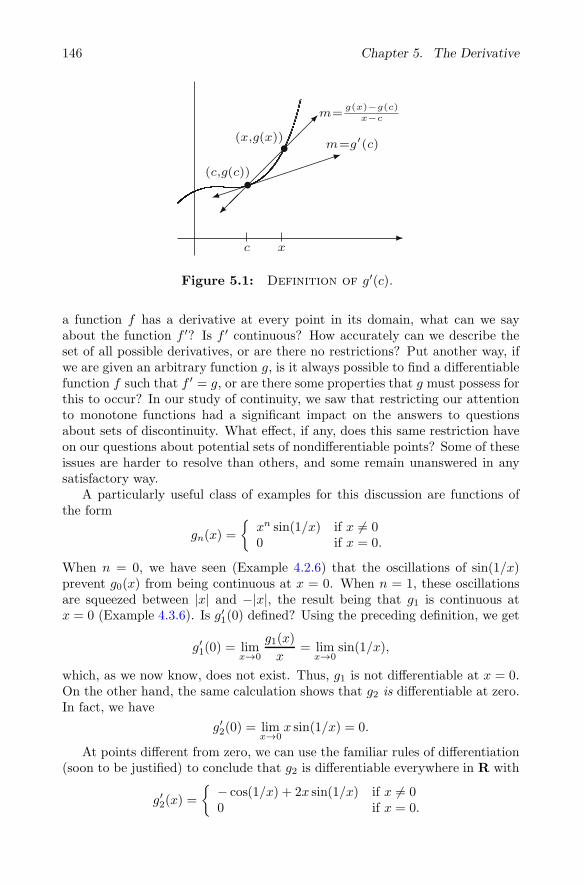
146 Chapter 5. The Derivative
(c,g(c))
(x,g(x))m=g′(c)
m= g(x)−g(c)x−c
c x
Figure 5.1: Definition of g′(c).
a function f has a derivative at every point in its domain, what can we sayabout the function f ′? Is f ′ continuous? How accurately can we describe theset of all possible derivatives, or are there no restrictions? Put another way, ifwe are given an arbitrary function g, is it always possible to find a differentiablefunction f such that f ′ = g, or are there some properties that g must possess forthis to occur? In our study of continuity, we saw that restricting our attentionto monotone functions had a significant impact on the answers to questionsabout sets of discontinuity. What effect, if any, does this same restriction haveon our questions about potential sets of nondifferentiable points? Some of theseissues are harder to resolve than others, and some remain unanswered in anysatisfactory way.
A particularly useful class of examples for this discussion are functions ofthe form
gn(x) =
{xn sin(1/x) if x �= 00 if x = 0.
When n = 0, we have seen (Example 4.2.6) that the oscillations of sin(1/x)prevent g0(x) from being continuous at x = 0. When n = 1, these oscillationsare squeezed between |x| and −|x|, the result being that g1 is continuous atx = 0 (Example 4.3.6). Is g′1(0) defined? Using the preceding definition, we get
g′1(0) = limx→0
g1(x)
x= lim
x→0sin(1/x),
which, as we now know, does not exist. Thus, g1 is not differentiable at x = 0.On the other hand, the same calculation shows that g2 is differentiable at zero.In fact, we have
g′2(0) = limx→0
x sin(1/x) = 0.
At points different from zero, we can use the familiar rules of differentiation(soon to be justified) to conclude that g2 is differentiable everywhere in R with
g′2(x) ={ − cos(1/x) + 2x sin(1/x) if x �= 0
0 if x = 0.

5.1. Discussion: Are Derivatives Continuous? 147
Figure 5.2: The function g2(x) = x2 sin(1/x) near zero.
But now consider
limx→0
g′2(x).
Because the cos(1/x) term is not preceded by a factor of x, we must concludethat this limit does not exist and that, consequently, the derivative functionis not continuous. To summarize, the function g2(x) is continuous and differ-entiable everywhere on R (Fig. 5.2), the derivative function g′2 is thus definedeverywhere on R, but g′2 has a discontinuity at zero. The conclusion is thatderivatives need not, in general, be continuous!
The discontinuity in g′2 is essential, meaning limx→0 g′(x) does not exist as a
one-sided limit. But, what about a function with a simple jump discontinuity?For example, does there exist a function h such that
h′(x) ={ −1 if x ≤ 0
1 if x > 0.
A first impression may bring to mind the absolute value function, which hasslopes of−1 at points to the left of zero and slopes of 1 to the right. However, theabsolute value function is not differentiable at zero. We are seeking a functionthat is differentiable everywhere, including the point zero, where we are insistingthat the slope of the graph be −1. The degree of difficulty of this request shouldstart to become apparent. Without sacrificing differentiability at any point, weare demanding that the slopes jump from −1 to 1 and not attain any value inbetween.
Although we have seen that continuity is not a required property of deriva-tives, the intermediate value property will prove a more stubborn quality toignore.

148 Chapter 5. The Derivative
5.2 Derivatives and the Intermediate
Value Property
Although the definition would technically make sense for more complicateddomains, all of the interesting results about the relationship between a func-tion and its derivative require that the domain of the given function be aninterval. Thinking geometrically of the derivative as a rate of change, it shouldnot be too surprising that we would want to confine the independent variableto move about a connected domain.
The theory of functional limits from Section 4.2 is all that is needed to supplya rigorous definition for the derivative.
Definition 5.2.1 (Differentiability). Let g : A → R be a function definedon an interval A. Given c ∈ A, the derivative of g at c is defined by
g′(c) = limx→c
g(x)− g(c)
x− c,
provided this limit exists. In this case we say g is differentiable at c. If g′ existsfor all points c ∈ A, we say that g is differentiable on A.
Example 5.2.2. (i) Consider f(x) = xn, where n ∈ N, and let c be anyarbitrary point in R. Using the algebraic identity
xn − cn = (x− c)(xn−1 + cxn−2 + c2xn−3 + · · ·+ cn−1),
we can calculate the familiar formula
f ′(c) = limx→c
xn − cn
x− c= lim
x→c(xn−1 + cxn−2 + c2xn−3 + · · ·+ cn−1)
= cn−1 + cn−1 + · · ·+ cn−1 = ncn−1.
(ii) If g(x) = |x|, then attempting to compute the derivative at c = 0 producesthe limit
g′(0) = limx→0
|x|x,
which is +1 or −1 depending on whether x approaches zero from the rightor left. Consequently, this limit does not exist, and we conclude that g isnot differentiable at zero.
Example 5.2.2 (ii) is a reminder that continuity of g does not imply that gis necessarily differentiable. On the other hand, if g is differentiable at a point,then it is true that g must be continuous at this point.
Theorem 5.2.3. If g : A → R is differentiable at a point c ∈ A, then g iscontinuous at c as well.

5.2. Derivatives and the Intermediate Value Property 149
Proof. We are assuming that
g′(c) = limx→c
g(x)− g(c)
x− c
exists, and we want to prove that limx→c g(x) = g(c). But notice that theAlgebraic Limit Theorem for functional limits allows us to write
limx→c
(g(x)− g(c)) = limx→c
(g(x)− g(c)
x− c
)
(x − c) = g′(c) · 0 = 0.
It follows that limx→c g(x) = g(c).
Combinations of Differentiable Functions
The Algebraic Limit Theorem (Theorem 2.3.3) led easily to the conclusionthat algebraic combinations of continuous functions are continuous. With onlyslightly more work, we arrive at a similar conclusion for sums, products, andquotients of differentiable functions.
Theorem 5.2.4 (Algebraic Differentiability Theorem). Let f and g befunctions defined on an interval A, and assume both are differentiable at somepoint c ∈ A. Then,
(i) (f + g)′(c) = f ′(c) + g′(c),
(ii) (kf)′(c) = kf ′(c), for all k ∈ R,
(iii) (fg)′(c) = f ′(c)g(c) + f(c)g′(c), and
(iv) (f/g)′(c) = g(c)f ′(c)−f(c)g′(c)
[g(c)]2 , provided that g(c) �= 0.
Proof. Statements (i) and (ii) are left as exercises. To prove (iii), we rewrite thedifference quotient as
(fg)(x) − (fg)(c)
x− c=
f(x)g(x) − f(x)g(c) + f(x)g(c)− f(c)g(c)
x− c
= f(x)
[g(x)− g(c)
x− c
]
+ g(c)
[f(x)− f(c)
x− c
]
.
Because f is differentiable at c, it is continuous there and thus limx→c f(x) =f(c). This fact, together with the functional-limit version of the Algebraic LimitTheorem (Theorem 4.2.4), justifies the conclusion
limx→c
(fg)(x)− (fg)(c)
x− c= f(c)g′(c) + f ′(c)g(c).
A similar proof of (iv) is possible, or we can use an argument based on thenext result. Each of these options is discussed in Exercise 5.2.3.

150 Chapter 5. The Derivative
The composition of two differentiable functions also fortunately results in an-other differentiable function. This fact is referred to as the Chain Rule. To dis-cover the proper formula for the derivative of the composition g ◦ f , we canwrite
(g ◦ f)′(c) = limx→c
g(f(x)) − g(f(c))
x− c= lim
x→c
g(f(x))− g(f(c))
f(x)− f(c)· f(x)− f(c)
x− c
= g′(f(c)) · f ′(c).
With a little polish, this string of equations could qualify as a proof except for thepesky fact that the f(x)−f(c) expression causes problems in the denominator iff(x) = f(c) for x values in arbitrarily small neighborhoods of c. (The functiong2(x) discussed in Section 5.1 exhibits this behavior near c = 0.) The upcomingproof of the Chain Rule manages to finesse this problem but in content is essen-tially the argument just given. Another approach is sketched in Exercise 5.2.4.
Theorem 5.2.5 (Chain Rule). Let f : A → R and g : B → R satisfyf(A) ⊆ B so that the composition g ◦ f is defined. If f is differentiable atc ∈ A and if g is differentiable at f(c) ∈ B, then g ◦ f is differentiable at c with(g ◦ f)′(c) = g′(f(c)) · f ′(c).
Proof. Because g is differentiable at f(c), we know that
g′(f(c)) = limy→f(c)
g(y)− g(f(c))
y − f(c).
Another way to assert this same fact is to let d(y) be the difference quotient
(1) d(y) =g(y)− g(f(c))
y − f(c),
and observe that limy→f(c) d(y) = g′(f(c)). At the moment, d(y) is not definedwhen y = f(c), but it should seem natural to declare that d(f(c)) = g′(f(c)),so that d is continuous at f(c).
Now, we come to the finesse. Equation (1) can be rewritten as
(2) g(y)− g(f(c)) = d(y)(y − f(c)).
Observe that this equation holds for all y ∈ B including y = f(c). Thus, weare free to substitute y = f(t) for any arbitrary t ∈ A. If t �= c, we can divideequation (2) by (t− c) to get
g(f(t))− g(f(c))
t− c= d(f(t))
(f(t) − f(c))
t− c
for all t �= c. Finally, taking the limit as t → c and applying the Algebraic LimitTheorem together with Theorem 4.3.9 yields the desired formula.

5.2. Derivatives and the Intermediate Value Property 151
f ′(c)=0
a c b
Figure 5.3: The Interior Extremum Theorem.
Darboux’s Theorem
One conclusion from this chapter’s introduction is that although continuity isnecessary for the derivative to exist, it is not the case that the derivative functionitself will always be continuous. Our specific example was g2(x) = x2 sin(1/x),where we set g2(0) = 0. By tinkering with the exponent of the leading x2 factor,it is possible to construct examples of differentiable functions with derivativesthat are unbounded, or twice-differentiable functions that have discontinuoussecond derivatives (Exercise 5.2.7). The underlying principle in all of theseexamples is that by controlling the size of the oscillations of the original function,we can make the corresponding oscillations of the slopes volatile enough toprevent the existence of the relevant limits.
It is significant that for this class of examples, the discontinuities that ariseare never simple jump discontinuities. (A precise definition of “jump discon-tinuity” is presented in Section 4.6.) We are now ready to confirm our earliersuspicions that although derivatives do not in general have to be continuous,they do possess the intermediate value property. (See Definition 4.5.3.) Thissurprising observation is a fairly straightforward corollary to the more obviousobservation that differentiable functions attain maximums and minimums onlyat points where the derivative is equal to zero (Fig. 5.3).
Theorem 5.2.6 (Interior Extremum Theorem). Let f be differentiable onan open interval (a, b). If f attains a maximum value at some point c ∈ (a, b)(i.e., f(c) ≥ f(x) for all x ∈ (a, b)), then f ′(c) = 0. The same is true if f(c) isa minimum value.
Proof. Because c is in the open interval (a, b), we can construct two sequences(xn) and (yn), which converge to c and satisfy xn < c < yn for all n ∈ N. Thefact that f(c) is a maximum implies that f(yn)− f(c) ≤ 0 for all n, and thus
f ′(c) = limn→∞
f(yn)− f(c)
yn − c≤ 0

152 Chapter 5. The Derivative
by the Order Limit Theorem (Theorem 2.3.4). In a similar way,
f(xn)− f(c)
xn − c≥ 0
for each xn because both numerator and denominator are negative. This impliesthat
f ′(c) = limn→∞
f(xn)− f(c)
xn − c≥ 0,
and therefore f ′(c) = 0, as desired.
The Interior Extremum Theorem is the fundamental fact behind the use ofthe derivative as a tool for solving applied optimization problems. This idea,discovered and exploited by Pierre de Fermat, is as old as the derivative itself.In a sense, finding maximums and minimums is arguably why Fermat inventedhis method of finding slopes of tangent lines. It was 200 years later that theFrench mathematician Gaston Darboux (1842–1917) pointed out that Fermat’smethod of finding maximums and minimums carries with it the implication thatif a derivative function attains two distinct values f ′(a) and f ′(b), then it mustalso attain every value in between.
Theorem 5.2.7 (Darboux’s Theorem). If f is differentiable on an interval[a, b], and if α satisfies f ′(a) < α < f ′(b) (or f ′(a) > α > f ′(b)), then thereexists a point c ∈ (a, b) where f ′(c) = α.
Proof. We first simplify matters by defining a new function g(x) = f(x) − αxon [a, b]. Notice that g is differentiable on [a, b] with g′(x) = f ′(x)−α. In termsof g, our hypothesis states that g′(a) < 0 < g′(b), and we hope to show thatg′(c) = 0 for some c ∈ (a, b).
The remainder of the argument is outlined in Exercise 5.2.11.
Exercises
Exercise 5.2.1. Supply proofs for parts (i) and (ii) of Theorem 5.2.4.
Exercise 5.2.2. Exactly one of the following requests is impossible. Decidewhich it is, and provide examples for the other three. In each case, let’s assumethe functions are defined on all of R.
(a) Functions f and g not differentiable at zero but where fg is differentiableat zero.
(b) A function f not differentiable at zero and a function g differentiable atzero where fg is differentiable at zero.
(c) A function f not differentiable at zero and a function g differentiable atzero where f + g is differentiable at zero.
(d) A function f differentiable at zero but not differentiable at any other point.

5.2. Derivatives and the Intermediate Value Property 153
Exercise 5.2.3. (a) Use Definition 5.2.1 to produce the proper formula forthe derivative of h(x) = 1/x.
(b) Combine the result in part (a) with the Chain Rule (Theorem 5.2.5) tosupply a proof for part (iv) of Theorem 5.2.4.
(c) Supply a direct proof of Theorem 5.2.4 (iv) by algebraically manipulat-ing the difference quotient for (f/g) in a style similar to the proof ofTheorem 5.2.4 (iii).
Exercise 5.2.4. Follow these steps to provide a slightly modified proof of theChain Rule.
(a) Show that a function h : A → R is differentiable at a ∈ A if and only ifthere exists a function l : A → R which is continuous at a and satisfies
h(x) − h(a) = l(x)(x− a) for all x ∈ A.
(b) Use this criterion for differentiability (in both directions) to prove Theorem5.2.5.
Exercise 5.2.5. Let fa(x) =
{xa if x > 00 if x ≤ 0.
(a) For which values of a is f continuous at zero?
(b) For which values of a is f differentiable at zero? In this case, is thederivative function continuous?
(c) For which values of a is f twice-differentiable?
Exercise 5.2.6. Let g be defined on an interval A, and let c ∈ A.
(a) Explain why g′(c) in Definition 5.2.1 could have been given by
g′(c) = limh→0
g(c+ h)− g(c)
h.
(b) Assume A is open. If g is differentiable at c ∈ A, show
g′(c) = limh→0
g(c+ h)− g(c− h)
2h.
Exercise 5.2.7. Let
ga(x) =
{xa sin(1/x) if x �= 00 if x = 0.
Find a particular (potentially noninteger) value for a so that
(a) ga is differentiable on R but such that g′a is unbounded on [0, 1].
154 Chapter 5. The Derivative
(b) ga is differentiable on R with g′a continuous but not differentiable at zero.
(c) ga is differentiable on R and g′a is differentiable on R, but such that g′′a isnot continuous at zero.
Exercise 5.2.8. Review the definition of uniform continuity (Definition 4.4.4).Given a differentiable function f : A → R, let’s say that f is uniformly differ-entiable on A if, given ε > 0 there exists a δ > 0 such that
∣∣∣∣f(x)− f(y)
x− y− f ′(y)
∣∣∣∣ < ε whenever 0 < |x− y| < δ.
(a) Is f(x) = x2 uniformly differentiable on R? How about g(x) = x3?
(b) Show that if a function is uniformly differentiable on an interval A, thenthe derivative must be continuous on A.
(c) Is there a theorem analogous to Theorem 4.4.7 for differentiation? Arefunctions that are differentiable on a closed interval [a, b] necessarily uni-formly differentiable?
Exercise 5.2.9. Decide whether each conjecture is true or false. Provide anargument for those that are true and a counterexample for each one that is false.
(a) If f ′ exists on an interval and is not constant, then f ′ must take on someirrational values.
(b) If f ′ exists on an open interval and there is some point c where f ′(c) > 0,then there exists a δ-neighborhood Vδ(c) around c in which f ′(x) > 0 forall x ∈ Vδ(c).
(c) If f is differentiable on an interval containing zero and if limx→0 f′(x) = L,
then it must be that L = f ′(0).
Exercise 5.2.10. Recall that a function f : (a, b) → R is increasing on (a, b)if f(x) ≤ f(y) whenever x < y in (a, b). A familiar mantra from calculus isthat a differentiable function is increasing if its derivative is positive, but thisstatement requires some sharpening in order to be completely accurate.
Show that the function
g(x) =
{x/2 + x2 sin(1/x) if x �= 00 if x = 0
is differentiable on R and satisfies g′(0) > 0. Now, prove that g is not increasingover any open interval containing 0.
In the next section we will see that f is indeed increasing on (a, b) if andonly if f ′(x) ≥ 0 for all x ∈ (a, b).
Exercise 5.2.11. Assume that g is differentiable on [a, b] and satisfies g′(a) <0 < g′(b).
(a) Show that there exists a point x ∈ (a, b) where g(a) > g(x), and a pointy ∈ (a, b) where g(y) < g(b).

5.3. The Mean Value Theorems 155
f ′(c)= f(b)−f(a)b−a(a,f(a))
(b,f(b))
a c b
Figure 5.4: The Mean Value Theorem.
(b) Now complete the proof of Darboux’s Theorem started earlier.
Exercise 5.2.12 (Inverse functions). If f : [a, b] → R is one-to-one, thenthere exists an inverse function f−1 defined on the range of f given by f−1(y) =x where y = f(x). In Exercise 4.5.8 we saw that if f is continuous on [a, b],then f−1 is continuous on its domain. Let’s add the assumption that f isdifferentiable on [a, b] with f ′(x) �= 0 for all x ∈ [a, b]. Show f−1 is differentiablewith
(f−1
)′(y) =
1
f ′(x)where y = f(x).
5.3 The Mean Value Theorems
The Mean Value Theorem (Fig. 5.4) makes the geometrically plausible assertionthat a differentiable function f on an interval [a, b] will, at some point, attain aslope equal to the slope of the line through the endpoints (a, f(a)) and (b, f(b)).More tersely put,
f ′(c) =f(b)− f(a)
b − a
for at least one point c ∈ (a, b).On the surface, there does not appear to be anything especially remarkable
about this observation. Its validity appears undeniable—much like the Inter-mediate Value Theorem for continuous functions—and its proof is rather short.The ease of the proof, however, is misleading, as it is built on top of somehard-fought accomplishments from the study of limits and continuity. In thisregard, the Mean Value Theorem is a kind of reward for a job well done. As wewill see, it is a prize of exceptional value. Although the result itself is geomet-rically unsurprising, the Mean Value Theorem is the cornerstone of the prooffor almost every major theorem pertaining to differentiation. We will use it toprove L’Hospital’s rules regarding limits of quotients of differentiable functions.
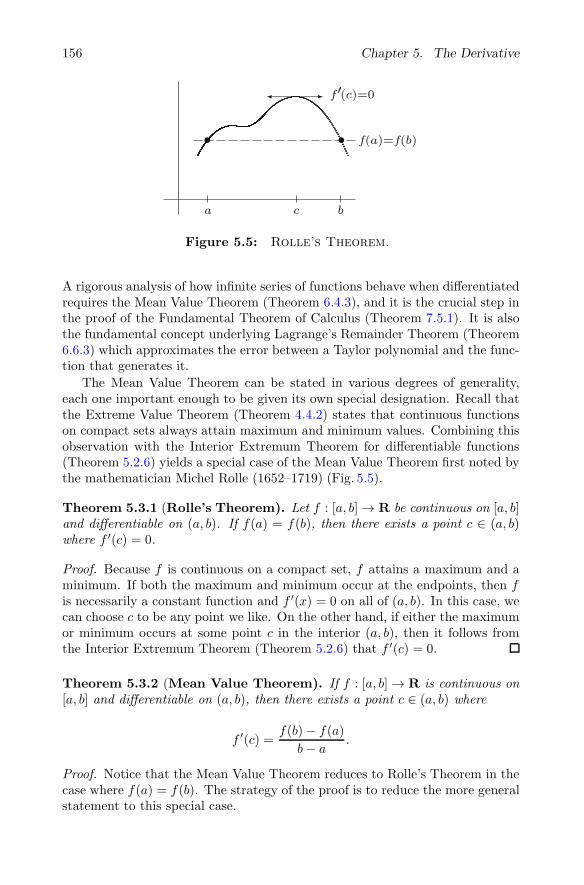
156 Chapter 5. The Derivative
�� f′(c)=0
f(a)=f(b)
a c b
Figure 5.5: Rolle’s Theorem.
A rigorous analysis of how infinite series of functions behave when differentiatedrequires the Mean Value Theorem (Theorem 6.4.3), and it is the crucial step inthe proof of the Fundamental Theorem of Calculus (Theorem 7.5.1). It is alsothe fundamental concept underlying Lagrange’s Remainder Theorem (Theorem6.6.3) which approximates the error between a Taylor polynomial and the func-tion that generates it.
The Mean Value Theorem can be stated in various degrees of generality,each one important enough to be given its own special designation. Recall thatthe Extreme Value Theorem (Theorem 4.4.2) states that continuous functionson compact sets always attain maximum and minimum values. Combining thisobservation with the Interior Extremum Theorem for differentiable functions(Theorem 5.2.6) yields a special case of the Mean Value Theorem first noted bythe mathematician Michel Rolle (1652–1719) (Fig. 5.5).
Theorem 5.3.1 (Rolle’s Theorem). Let f : [a, b] → R be continuous on [a, b]and differentiable on (a, b). If f(a) = f(b), then there exists a point c ∈ (a, b)where f ′(c) = 0.
Proof. Because f is continuous on a compact set, f attains a maximum and aminimum. If both the maximum and minimum occur at the endpoints, then fis necessarily a constant function and f ′(x) = 0 on all of (a, b). In this case, wecan choose c to be any point we like. On the other hand, if either the maximumor minimum occurs at some point c in the interior (a, b), then it follows fromthe Interior Extremum Theorem (Theorem 5.2.6) that f ′(c) = 0.
Theorem 5.3.2 (Mean Value Theorem). If f : [a, b] → R is continuous on[a, b] and differentiable on (a, b), then there exists a point c ∈ (a, b) where
f ′(c) =f(b)− f(a)
b− a.
Proof. Notice that the Mean Value Theorem reduces to Rolle’s Theorem in thecase where f(a) = f(b). The strategy of the proof is to reduce the more generalstatement to this special case.

5.3. The Mean Value Theorems 157
The equation of the line through (a, f(a)) and (b, f(b)) is
y =
(f(b)− f(a)
b− a
)
(x− a) + f(a).
•
•d(x)
{
(a,f(a))
(b,f(b))
a x b
We want to consider the difference between this line and the function f(x). Tothis end, let
d(x) = f(x)−[(
f(b)− f(a)
b− a
)
(x− a) + f(a)
]
,
and observe that d is continuous on [a, b], differentiable on (a, b), and satisfiesd(a) = 0 = d(b). Thus, by Rolle’s Theorem, there exists a point c ∈ (a, b) whered′(c) = 0. Because
d′(x) = f ′(x) − f(b)− f(a)
b− a,
we get
0 = f ′(c)− f(b)− f(a)
b− a,
which completes the proof.
The point has been made that the Mean Value Theorem manages to find itsway into nearly every proof of any statement related to the geometrical natureof the derivative. As a simple example, if f is a constant function f(x) = k onsome interval A, then a straightforward calculation of f ′ using Definition 5.2.1shows that f ′(x) = 0 for all x ∈ A. But how do we prove the converse statement?If we know that a differentiable function g satisfies g′(x) = 0 everywhere on A,our intuition suggests that we should be able to prove g(x) is constant. It is theMean Value Theorem that provides us with a way to articulate rigorously whatseems geometrically valid.
Corollary 5.3.3. If g : A → R is differentiable on an interval A and satisfiesg′(x) = 0 for all x ∈ A, then g(x) = k for some constant k ∈ R.
Proof. Take x, y ∈ A and assume x < y. Applying the Mean Value Theorem tog on the interval [x, y], we see that
g′(c) =g(y)− g(x)
y − x

158 Chapter 5. The Derivative
for some c ∈ A. Now, g′(c) = 0, so we conclude that g(y) = g(x). Set k equalto this common value. Because x and y are arbitrary, it follows that g(x) = kfor all x ∈ A.
Corollary 5.3.4. If f and g are differentiable functions on an interval A andsatisfy f ′(x) = g′(x) for all x ∈ A, then f(x) = g(x) + k for some constantk ∈ R.
Proof. Let h(x) = f(x) − g(x) and apply Corollary 5.3.3 to the differentiablefunction h.
The Mean Value Theorem has a more general form due to Cauchy. It is thisgeneralized version of the theorem that is needed to analyze L’Hospital’s rulesand Lagrange’s Remainder Theorem.
Theorem 5.3.5 (Generalized Mean Value Theorem). If f and g are con-tinuous on the closed interval [a, b] and differentiable on the open interval (a, b),then there exists a point c ∈ (a, b) where
[f(b)− f(a)]g′(c) = [g(b)− g(a)]f ′(c).
If g′ is never zero on (a, b), then the conclusion can be stated as
f ′(c)g′(c)
=f(b)− f(a)
g(b)− g(a).
Proof. This result follows by applying the Mean Value Theorem to the func-tion h(x) = [f(b) − f(a)]g(x) − [g(b) − g(a)]f(x). The details are requested inExercise 5.3.5.
L’Hospital’s Rules
The Algebraic Limit Theorem asserts that when taking a limit of a quotient offunctions we can write
limx→c
f(x)
g(x)=
limx→c
f(x)
limx→c
g(x),
provided that each individual limit exists and limx→c g(x) is not zero. If thedenominator does converge to zero and the numerator has a nonzero limit,then it is not difficult to argue that the quotient f(x)/g(x) grows in absolutevalue without bound as x approaches c. L’Hospital’s Rules are named for theMarquis de L’Hospital (1661–1704), who learned the results from his tutor,Johann Bernoulli (1667–1748), and published them in 1696 in what is regardedas the first calculus text. Stated in different levels of generality, they are aneffective tool for handling the indeterminant cases when either numerator anddenominator both tend to zero or both tend simultaneously to infinity.

5.3. The Mean Value Theorems 159
Theorem 5.3.6 (L’Hospital’s Rule: 0/0 case). Let f and g be continuouson an interval containing a, and assume f and g are differentiable on thisinterval with the possible exception of the point a. If f(a) = g(a) = 0 andg′(x) �= 0 for all x �= a, then
limx→a
f ′(x)g′(x)
= L implies limx→a
f(x)
g(x)= L.
Proof. This argument follows from a straightforward application of the Gener-alized Mean Value Theorem. It is requested as Exercise 5.3.11.
L’Hospital’s Rule remains true if we replace the assumption that f(a) =g(a) = 0 with the hypothesis that limx→a g(x) = ∞. To this point we have notbeen explicit about what it means to say that a limit equals ∞. The logicalstructure of such a definition is precisely the same as it is for finite functionallimits. The difference is that rather than trying to force the function to takeon values in some small ε-neighborhood around a proposed limit, we must showthat g(x) eventually exceeds any proposed upper bound. The arbitrarily smallε > 0 is replaced by an arbitrarily large M > 0.
Definition 5.3.7. Given g : A → R and a limit point c of A, we say thatlimx→c g(x) = ∞ if, for every M > 0, there exists a δ > 0 such that whenever0 < |x− c| < δ it follows that g(x) ≥ M .
We can define limx→c g(x) = −∞ in a similar way.
The following version of L’Hospital’s Rule is typically referred to as the∞/∞case even though the hypothesis only requires that the function in the denomi-nator tend to infinity. To simplify the notation of the proof, we state the resultusing a one-sided limit.
Theorem 5.3.8 (L’Hospital’s Rule: ∞/∞ case). Assume f and g aredifferentiable on (a, b) and that g′(x) �= 0 for all x ∈ (a, b). If limx→a g(x) = ∞(or −∞), then
limx→a
f ′(x)g′(x)
= L implies limx→a
f(x)
g(x)= L.
Proof. Let ε > 0. Because limx→af ′(x)g′(x) = L, there exists a δ1 > 0 such that
∣∣∣∣f ′(x)g′(x)
− L
∣∣∣∣ <
ε
2
for all a < x < a+ δ1. For convenience of notation, let t = a+ δ1 and note thatt is fixed for the remainder of the argument.
Our functions are not defined at a, but for any x ∈ (a, t) we can apply theGeneralized Mean Value Theorem on the interval [x, t] to get
f(x)− f(t)
g(x)− g(t)=
f ′(c)g′(c)

160 Chapter 5. The Derivative
for some c ∈ (x, t). Our choice of t then implies
(1) L− ε
2<
f(x)− f(t)
g(x)− g(t)< L+
ε
2
for all x in (a, t).
In an effort to isolate the fraction f(x)g(x) , the strategy is to multiply inequality
(1) by (g(x) − g(t))/g(x). We need to be sure, however, that this quantity ispositive, which amounts to insisting that 1 ≥ g(t)/g(x). Because t is fixed andlimx→a g(x) = ∞, we can choose δ2 > 0 so that g(x) ≥ g(t) for all a < x < a+δ2.Carrying out the desired multiplication results in
(L− ε
2
)(
1− g(t)
g(x)
)
<f(x)− f(t)
g(x)<
(L+
ε
2
)(
1− g(t)
g(x)
)
,
which after some algebraic manipulations yields
L− ε
2+
−Lg(t) + ε2g(t) + f(t)
g(x)<
f(x)
g(x)< L+
ε
2+
−Lg(t)− ε2g(t) + f(t)
g(x).
Again, let’s remind ourselves that t is fixed and that limx→a g(x) = ∞. Thus,we can choose a δ3 such that a < x < a + δ3 implies that g(x) is large enoughto ensure that both
−Lg(t) + ε2g(t) + f(t)
g(x)and
−Lg(t)− ε2g(t) + f(t)
g(x)
are less than ε/2 in absolute value. Putting this all together and choosingδ = min{δ1, δ2, δ3} guarantees that
∣∣∣∣f(x)
g(x)− L
∣∣∣∣ < ε
for all a < x < a+ δ.
Exercises
Exercise 5.3.1. Recall from Exercise 4.4.9 that a function f : A → R isLipschitz on A if there exists an M > 0 such that
∣∣∣∣f(x)− f(y)
x− y
∣∣∣∣ ≤ M
for all x �= y in A.
(a) Show that if f is differentiable on a closed interval [a, b] and if f ′ is con-tinuous on [a, b], then f is Lipschitz on [a, b].
(b) Review the definition of a contractive function in Exercise 4.3.11. If weadd the assumption that |f ′(x)| < 1 on [a, b], does it follow that f iscontractive on this set?

5.3. The Mean Value Theorems 161
Exercise 5.3.2. Let f be differentiable on an interval A. If f ′(x) �= 0 on A,show that f is one-to-one on A. Provide an example to show that the conversestatement need not be true.
Exercise 5.3.3. Let h be a differentiable function defined on the interval [0, 3],and assume that h(0) = 1, h(1) = 2, and h(3) = 2.
(a) Argue that there exists a point d ∈ [0, 3] where h(d) = d.
(b) Argue that at some point c we have h′(c) = 1/3.
(c) Argue that h′(x) = 1/4 at some point in the domain.
Exercise 5.3.4. Let f be differentiable on an interval A containing zero, andassume (xn) is a sequence in A with (xn) → 0 and xn �= 0.
(a) If f(xn) = 0 for all n ∈ N , show f(0) = 0 and f ′(0) = 0.
(b) Add the assumption that f is twice-differentiable at zero and show thatf ′′(0) = 0 as well.
Exercise 5.3.5. (a) Supply the details for the proof of Cauchy’s GeneralizedMean Value Theorem (Theorem 5.3.5).
(b) Give a graphical interpretation of the Generalized Mean Value Theoremanalogous to the one given for the Mean Value Theorem at the beginningof Section 5.3. (Consider f and g as parametric equations for a curve.)
Exercise 5.3.6. (a) Let g : [0, a] → R be differentiable, g(0) = 0, and|g′(x)| ≤ M for all x ∈ [0, a]. Show |g(x)| ≤ Mx for all x ∈ [0, a].
(b) Let h : [0, a] → R be twice differentiable, h′(0) = h(0) = 0 and |h′′(x)| ≤M for all x ∈ [0, a]. Show |h(x)| ≤ Mx2/2 for all x ∈ [0, a].
(c) Conjecture and prove an analogous result for a function that is differen-tiable three times on [0, a].
Exercise 5.3.7. A fixed point of a function f is a value x where f(x) = x.Show that if f is differentiable on an interval with f ′(x) �= 1, then f can haveat most one fixed point.
Exercise 5.3.8. Assume f is continuous on an interval containing zero anddifferentiable for all x �= 0. If limx→0 f
′(x) = L, show f ′(0) exists and equals L.
Exercise 5.3.9. Assume f and g are as described in Theorem 5.3.6, but nowadd the assumption that f and g are differentiable at a, and f ′ and g′ arecontinuous at a with g′(a) �= 0. Find a short proof for the 0/0 case of L’Hospital’sRule under this stronger hypothesis.

162 Chapter 5. The Derivative
Exercise 5.3.10. Let f(x) = x sin(1/x4)e−1/x2
and g(x) = e−1/x2
. Using thefamiliar properties of these functions, compute the limit as x approaches zero off(x), g(x), f(x)/g(x), and f ′(x)/g′(x). Explain why the results are surprisingbut not in conflict with the content of Theorem 5.3.6.1
Exercise 5.3.11. (a) Use the Generalized Mean Value Theorem to furnish aproof of the 0/0 case of L’Hospital’s Rule (Theorem 5.3.6).
(b) If we keep the first part of the hypothesis of Theorem 5.3.6 the same butwe assume that
limx→a
f ′(x)g′(x)
= ∞,
does it necessarily follow that
limx→a
f(x)
g(x)= ∞?
Exercise 5.3.12. If f is twice differentiable on an open interval containing aand f ′′ is continuous at a, show
limh→0
f(a+ h)− 2f(a) + f(a− h)
h2= f ′′(a).
(Compare this to Exercise 5.2.6(b).)
5.4 A Continuous Nowhere-DifferentiableFunction
Exploring the relationship between continuity and differentiability has led toboth fruitful results and pathological counterexamples. The bulk of discussionto this point has focused on the continuity of derivatives, but historically a sig-nificant amount of debate revolved around the question of whether continuousfunctions were necessarily differentiable. Early in the chapter, we saw that con-tinuity was a requirement for differentiability, but, as the absolute value functiondemonstrates, the converse of this proposition is not true. A function can becontinuous but not differentiable at some point. But just how nondifferentiablecan a continuous function be? Given a finite set of points, it is not difficult toimagine how to construct a graph with corners at each of these points, so thatthe corresponding function fails to be differentiable on this finite set. The trickgets more difficult, however, when the set becomes infinite. For instance, is itpossible to construct a function that is continuous on all of R but fails to bedifferentiable at every rational point? Not only is this possible, but the situationis even more disconcerting. In 1872, Karl Weierstrass presented an example ofa continuous function that was not differentiable at any point. (It seems to be
1A large class of “counterexamples” of this sort to L’Hospital’s Rule are explored in [4].

5.4. A Continuous Nowhere-Differentiable Function 163
1
−2 −1 321
Figure 5.6: The function h(x).
the case that Bernhard Bolzano had his own example of such a beast as earlyas 1830, but it was not published until much later.)
Weierstrass actually discovered a class of nowhere-differentiable functions ofthe form
f(x) =
∞∑
n=0
an cos(bnx)
where the values of a and b are carefully chosen. Such functions are specificexamples of Fourier series discussed in Section 8.5. The details of Weierstrass’argument are simplified if we replace the cosine function with a piecewise linearfunction that has oscillations qualitatively like cos(x).
Define
h(x) = |x|on the interval [−1, 1] and extend the definition of h to all of R by requiringthat h(x+ 2) = h(x). The result is a periodic “sawtooth” function (Fig. 5.6).
Exercise 5.4.1. Sketch a graph of (1/2)h(2x) on [−2, 3]. Give a qualitativedescription of the functions
hn(x) =1
2nh(2nx)
as n gets larger.
Now, define
g(x) =
∞∑
n=0
hn(x) =
∞∑
n=0
1
2nh(2nx).
The claim is that g(x) is continuous on all of R but fails to be differentiable atany point.
Infinite Series of Functions and Continuity
The definition of g(x) is a significant departure from the way we usually definefunctions. For each x ∈ R, g(x) is defined to be the value of an infinite series.

164 Chapter 5. The Derivative
21–1
Figure 5.7: A sketch of g(x) =∑∞
n=0(1/2n)h(2nx).
Exercise 5.4.2. Fix x ∈ R. Argue that the series
∞∑
n=0
1
2nh(2nx)
converges and thus g(x) is properly defined.
Exercise 5.4.3. Taking the continuity of h(x) as given, reference the propertheorems from Chapter 4 that imply that the finite sum
gm(x) =
m∑
n=0
1
2nh(2nx)
is continuous on R.
This brings us to an archetypical question in analysis: When do conclusionsthat are valid in finite settings extend to infinite ones? A finite sum of continuousfunctions is certainly continuous, but does this necessarily hold for an infinitesum of continuous functions? In general, we will see that this is not always thecase. For this particular sum, however, the continuity of the limit function g(x)can be proved. Deciphering when results about finite sums of functions extendto infinite sums is one of the fundamental themes of Chapter 6. Although aself-contained argument for the continuity of g is not beyond our means at thispoint, we will nevertheless postpone the proof (see, for example, Exercise 6.4.3),leaving it as an enticement for the upcoming study of uniform convergence.
Exercise 5.4.4. As the graph in Figure 5.7 suggests, the structure of g(x) isquite intricate. Answer the following questions, assuming that g(x) is indeedcontinuous.
(a) How do we know g attains a maximum value M on [0, 2]? What is thisvalue?

5.4. A Continuous Nowhere-Differentiable Function 165
(b) Let D be the set of points in [0, 2] where g attains its maximum. That isD = {x ∈ [0, 2] : g(x) = M}. Find one point in D.
(c) Is D finite, countable, or uncountable?
Nondifferentiability
When the proper tools are in place, the proof that g is continuous is quitestraightforward. The more difficult task is to show that g is not differentiableat any point in R.
Let’s first look at the point x = 0. Our function g does not appear tobe differentiable here, and a rigorous proof is not too difficult. Consider thesequence xm = 1/2m, where m = 0, 1, 2, . . . .
Exercise 5.4.5. Show that
g(xm)− g(0)
xm − 0= m+ 1,
and use this to prove that g′(0) does not exist.
Any temptation to say something like g′(0) = ∞ should be resisted. Settingxm = −(1/2m) in the previous argument produces difference quotients headingtoward −∞. The geometric manifestation of this is the “cusp” that appears atx = 0 in the graph of g.
Exercise 5.4.6. (a) Modify the previous argument to show that g′(1) doesnot exist. Show that g′(1/2) does not exist.
(b) Show that g′(x) does not exist for any rational number of the form x =p/2k where p ∈ Z and k ∈ N ∪ {0}.
The points described in Exercise 5.4.6 (b) are called dyadic points. If x =p/2k is a dyadic rational number, then the function hn has a corner at x as longas n ≥ k. Thus, it should not be too surprising that g fails to be differentiableat points of this form. The argument is more delicate at points between thedyadic points.
Assume x is not a dyadic number. For a fixed value of m ∈ N ∪ {0}, x fallsbetween two adjacent dyadic points,
pm2m
< x <pm + 1
2m.
Set xm = pm/2m and ym = (pm + 1)/2m. Repeating this for each m yields twosequences (xm) and (ym) satisfying
limxm = lim ym = x and xm < x < ym.

166 Chapter 5. The Derivative
Exercise 5.4.7. (a) First prove the following general lemma: Let f be definedon an open interval J and assume f is differentiable at a ∈ J . If (an) and (bn)are sequences satisfying an < a < bn and lim an = lim bn = a, show
f ′(a) = limn→∞
f(bn)− f(an)
bn − an.
(b) Now use this lemma to show that g′(x) does not exist.
Weierstrass’s original 1872 paper contained a demonstration that the infinitesum
f(x) =
∞∑
n=0
an cos(bnx)
defined a continuous nowhere-differentiable function provided 0 < a < 1 andb was an odd integer satisfying ab > 1 + 3π/2. The condition on a is easy tounderstand. If 0 < a < 1, then
∑∞n=0 a
n is a convergent geometric series, andthe forthcoming Weierstrass M-Test (Theorem 6.4.5) can be used to concludethat f is continuous. The restriction on b is more mysterious. In 1916, G.H.Hardy extended Weierstrass’ result to include any value of b for which ab ≥ 1.Without looking at the details of either of these arguments, we nevertheless geta sense that the lack of a derivative is intricately tied to the relationship betweenthe compression factor (the parameter a) and the rate at which the frequencyof the oscillations increases (the parameter b).
Exercise 5.4.8. Review the argument for the nondifferentiability of g(x) atnondyadic points. Does the argument still work if we replace g(x) with thesummation
∑∞n=0(1/2
n)h(3nx)? Does the argument work for the function∑∞n=0(1/3
n)h(2nx)?
5.5 Epilogue
Far from being an anomaly to be relegated to the margins of our understandingof continuous functions, Weierstrass’s example and those like it should actuallyserve as a guide to our intuition. The image of continuity as a smooth curvein our mind’s eye severely misrepresents the situation and is the result of abias stemming from an overexposure to the much smaller class of differentiablefunctions. The lesson here is that continuity is a strictly weaker notion thandifferentiability. In Section 3.6, we alluded to a corollary of the Baire CategoryTheorem, which asserts that Weierstrass’s construction is actually typical ofcontinuous functions. We will see that most continuous functions are nowhere-differentiable, so that it is really the differentiable functions that are the excep-tions rather than the rule. The details of how to phrase this observation morerigorously are spelled out in Section 8.2.
To say that the nowhere-differentiable function g constructed in the previoussection has “corners” at every point of its domain misses the mark. Weierstrass’soriginal class of nowhere-differentiable functions was constructed from infinite
5.5. Epilogue 167
sums of smooth trigonometric functions. It is the densely nested oscillatingstructure that makes the definition of a tangent line impossible. So what hap-pens when we restrict our attention to monotone functions? How nondifferen-tiable can an increasing function be? Given a finite set of points, it is not difficultto piece together a monotone function which has actual corners—and thus isnot differentiable—at each point in the given set. A natural question is whetherthere exists a continuous, monotone function that is nowhere-differentiable.Weierstrass suspected that such a function existed but only managed to producean example of a continuous, increasing function which failed to be differentiableon a countable dense set (Exercise 7.5.11). In 1903, the French mathemati-cian Henri Lebesgue (1875–1941) demonstrated that Weierstrass’s intuition hadfailed on this account. Lebesgue proved that a continuous, monotone functionwould have to be differentiable at “almost” every point in its domain. To bespecific, Lebesgue showed that, for every ε > 0, the set of points where such afunction fails to be differentiable can be covered by a countable union of inter-vals whose lengths sum to less than ε. This notion of “zero length,” or “measurezero” as it is called, was encountered in our discussion of the Cantor set and isexplored more fully in Section 7.6, where Lebesgue’s substantial contribution tothe theory of integration is discussed.
With the relationship between the continuity of f and the existence of f ′
somewhat in hand, we once more return to the question of characterizing the setof all derivatives. Not every function is a derivative. Darboux’s Theorem forcesus to conclude that there are some functions—those with jump discontinuitiesin particular—that cannot appear as the derivative of some other function.Another way to phrase Darboux’s Theorem is to say that all derivatives mustsatisfy the intermediate value property. Continuous functions do possess theintermediate value property, and it is natural to ask whether every continuousfunction is necessarily a derivative. For this smaller class of functions, theanswer is yes. The Fundamental Theorem of Calculus, treated in Chapter 7,states that, given a continuous function f , the function F (x) =
∫ x
af satisfies
F ′ = f . This does the trick. The collection of derivatives at least contains thecontinuous functions. The search for a concise characterization of all possiblederivatives, however, remains largely unsuccessful.
As a final remark, we will see that by cleverly choosing f , this techniqueof defining F via F (x) =
∫ x
a f can be used to produce examples of continuousfunctions which fail to be differentiable on interesting sets, provided we can showthat
∫ x
a f is defined. The question of just how to define integration became acentral theme in analysis in the latter half of the 19th century and has continuedon to the present. Much of this story is discussed in detail in Chapter 7 andSection 8.1.

Chapter 6
Sequences and Seriesof Functions
6.1 Discussion: The Power of Power Series
In 1689, Jakob Bernoulli published his Tractatus de seriebus infinitis summa-rizing what was known about infinite series toward the end of the 17th century.Full of clever calculations and conclusions, this publication was also notable forone particular question that it didn’t answer; namely, what is the precise valueof the series ∞∑
n=1
1
n2= 1 +
1
4+
1
9+
1
16+ · · · .
Bernoulli convincingly argued that∑
1/n2 converged to something less than2 (see Example 2.4.4) but he was unable to find an explicit expression forthe limit. Generally speaking, it is much harder to sum a series than it is todetermine whether or not it converges. In fact, being able to find the sum of aconvergent series is the exception rather than the rule. In this case, however, theseries
∑1/n2 seemed so elementary; more elementary than, say,
∑∞n=1 n
2/2n or∑∞n=1 1/n(n+ 1), both of which Bernoulli was able to handle. “If anyone finds
and communicates to us that which has so far eluded our efforts,” Bernoulliwrote, “great will be our gratitude.”1
Geometric series are the most prominent class of examples that can be readilysummed. In Example 2.7.5 we proved that
(1)1
1− x= 1 + x+ x2 + x3 + · · ·
1As quoted in [12], which contains a much more thorough account of this story.
© Springer Science+Business Media New York 2015S. Abbott, Understanding Analysis, Undergraduate Textsin Mathematics, DOI 10.1007/978-1-4939-2712-8 6
169

170 Chapter 6. Sequences and Series of Functions
for all |x| < 1. Thus, for example,∑∞
n=0 1/2n = 2 and
∑∞n=0(−1/3)n = 3/4.
Geometric series were part of mathematical folklore long before Bernoulli; how-ever, what was relatively novel in Bernoulli’s time was the idea of operating oninfinite series such as (1) with tools from the budding theory of calculus. Forinstance, what happens if we take the derivative on each side of equation (1)?The left side is easy enough—we just get 1/(1− x)2. But what about the rightside? Adopting a 17th century mindset, a natural way to proceed is to treat theinfinite series as a polynomial, albeit of infinite degree. Differentiation acrossequation (1) in this fashion gives
(2)1
(1− x)2= 0 + 1 + 2x+ 3x2 + 4x3 + · · · .
Is this a valid formula, at least for values of x in (−1, 1)? Empirical evidencesuggests it is. Setting x = 1/2 we get
4 =∞∑
n=1
n
2n−1= 1 + 1 +
3
4+
4
8+
5
16+ · · · ,
which feels plausible, and is in fact true. Although not Bernoulli’s requestedseries, this does suggest a possible new line of attack.
Manipulations of this sort can be used to create a wide assortment of newseries representations for familiar functions. Substituting −x2 for x in (1) gives
(3)1
1 + x2= 1− x2 + x4 − x6 + x8 − · · · ,
for all x ∈ (−1, 1).Once again closing our eyes to the potential danger of treating an infinite
series as though it were a polynomial, let’s see what happens when we takeantiderivatives. Using the fact that
(arctan(x))′=
1
1 + x2and arctan(0) = 0,
equation (3) becomes
(4) arctan(x) = x− x3
3+
x5
5− x7
7+ · · · .
Plugging x = 1 into equation (4) yields the striking relationship
(5)π
4= 1− 1
3+
1
5− 1
7+
1
9− · · · .
The constant π, which arises from the geometry of circles, has somehow found itsway into an equation involving the reciprocals of the odd integers. Is this a validformula? Can we really treat the infinite series in (3) like a finite polynomial?Even if the answer is yes there is still another mystery to solve in this example.

6.1. Discussion: The Power of Power Series 171
Plugging x = 1 into equations (1), (2), or (3) yields mathematical gibberish, sois it prudent to anticipate something meaningful arising from equation (4) atthis same value? Will any of these ideas get us closer to computing
∑∞n=1 1/n
2?
As it turned out, Bernoulli’s plea for help was answered in an unexpected wayby Leonard Euler. At a young age, Euler was a student of Jakob Bernoulli’sbrother Johann, and the stellar pupil quickly rose to become the preeminentmathematician of his age. Euler’s solution is impossible to anticipate. In 1735,he announced that
1 +1
4+
1
9+
1
16+ · · · = π2
6,
a provocative formula that, even more than equation (5), hints at deep con-nections between geometry, number theory and analysis. Euler’s argument isquite short, but it needs to be viewed in the context of the time in which it wascreated. The “infinite polynomials” in this discussion are examples of powerseries, and a major catalyst for the expanding power of calculus in the 17th and18th centuries was a proliferation of techniques like the ones used to generateformulas (2), (3), and (4). The machinations of both algebra and calculus arerelatively straightforward when restricted to the class of polynomials. So, ifin fact power series could be treated more or less like unending polynomials,then there was a great incentive to try to find power series representations forfamiliar functions like ex,
√1 + x, or sin(x).
The appearance of arctan(x) in (4) is an encouraging sign that this mightindeed always be possible. One of Isaac Newton’s more significant achievementswas to produce a generalization of the binomial formula. If n ∈ N, then old-fashioned finite algebra leads to the formula
(1 + x)n = 1 + nx+n(n− 1)
2!x2 +
n(n− 1)(n− 2)
3!x3 + · · ·+ xn.
Through a process of experimentation and intuition Newton realized that forr /∈ N, the infinite series
(1 + x)r = 1 + rx +r(r − 1)
2!x2 +
r(r − 1)(r − 2)
3!x3 + · · ·
was meaningful, at least for x ∈ (−1, 1). Setting r = −1, for example, yields
1
1 + x= 1− x+ x2 − x3 + x4 − · · · ,
which is easily seen to be equivalent to equation (1). Setting r = 1/2 we get
√1 + x = 1 +
1
2x− 1
222!x2 +
3
233!x3 − 3 · 5
244!x4 + · · · .
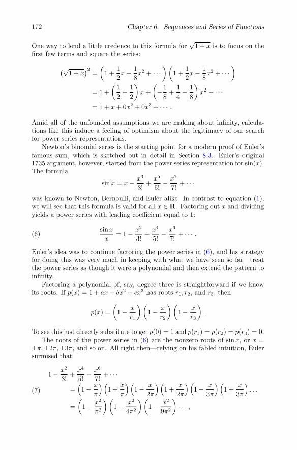
172 Chapter 6. Sequences and Series of Functions
One way to lend a little credence to this formula for√1 + x is to focus on the
first few terms and square the series:
(√1 + x
)2=
(
1 +1
2x− 1
8x2 + · · ·
)(
1 +1
2x− 1
8x2 + · · ·
)
= 1 +
(1
2+
1
2
)
x+
(
−1
8+
1
4− 1
8
)
x2 + · · ·
= 1 + x+ 0x2 + 0x3 + · · · .
Amid all of the unfounded assumptions we are making about infinity, calcula-tions like this induce a feeling of optimism about the legitimacy of our searchfor power series representations.
Newton’s binomial series is the starting point for a modern proof of Euler’sfamous sum, which is sketched out in detail in Section 8.3. Euler’s original1735 argument, however, started from the power series representation for sin(x).The formula
sinx = x− x3
3!+
x5
5!− x7
7!+ · · ·
was known to Newton, Bernoulli, and Euler alike. In contrast to equation (1),we will see that this formula is valid for all x ∈ R. Factoring out x and dividingyields a power series with leading coefficient equal to 1:
(6)sinx
x= 1− x2
3!+
x4
5!− x6
7!+ · · · .
Euler’s idea was to continue factoring the power series in (6), and his strategyfor doing this was very much in keeping with what we have seen so far—treatthe power series as though it were a polynomial and then extend the pattern toinfinity.
Factoring a polynomial of, say, degree three is straightforward if we knowits roots. If p(x) = 1 + ax+ bx2 + cx3 has roots r1, r2, and r3, then
p(x) =
(
1− x
r1
)(
1− x
r2
)(
1− x
r3
)
.
To see this just directly substitute to get p(0) = 1 and p(r1) = p(r2) = p(r3) = 0.
The roots of the power series in (6) are the nonzero roots of sinx, or x =±π,±2π,±3π, and so on. All right then—relying on his fabled intuition, Eulersurmised that
(7)
1− x2
3!+
x4
5!− x6
7!+ · · ·
=(1− x
π
)(1 +
x
π
)(1− x
2π
)(1 +
x
2π
)(1− x
3π
)(1 +
x
3π
). . .
=
(
1− x2
π2
)(
1− x2
4π2
)(
1− x2
9π2
)
· · · ,

6.2. Uniform Convergence of a Sequence of Functions 173
where in the last step adjacent pairs of factors have been multiplied together.What happens if we continue to multiply out the factors on the right? Well,the constant term comes out to be 1 which happily matches the constant termon the left. The magic comes when we compare the x2 term on each sideof (7). Multiplying out the infinite number of factors on the right (using ourimagination as necessary) and collecting like powers of x, equation (7) becomes
1− x2
3!+
x4
5!− x6
7!+ · · ·
= 1 +
(
− 1
π2− 1
4π2− 1
9π2− · · ·
)
x2 +
(1
4π4+
1
9π4+ · · ·
)
x4 + · · · .
Equating the coefficients of x2 on each side yields
− 1
3!= − 1
π2− 1
4π2− 1
9π2− · · · ,
which when we multiply by −π2 becomes
π2
6= 1 +
1
4+
1
9+
1
16+ · · · .
Numerical approximations of each side of this equation confirmed for Eulerthat, despite the audacious leaps in his argument, he had landed on solid ground.By our standards, this derivation falls well short of being a proper proof, andwe will have to tend to this in the upcoming chapters. The takeaway of thisdiscussion is that the hard work ahead is worth the effort. Infinite series repre-sentations of functions are both useful and surprisingly elegant, and can lead toremarkable conclusions when they are properly handled.
The evidence so far suggests power series are quite robust when treated asif they were finite in nature. Term-by-term differentiation produced a validconclusion in equation (2), and taking antiderivatives fared similarly well in(4). We will see that these manipulations are not always justified for infiniteseries of more general types of functions. What is it about power series inparticular that makes them so impervious to the dangers of the infinite? Ofthe many unanswered questions in this discussion, this last one is probably themost central, and the most important to understanding series of functions ingeneral.
6.2 Uniform Convergence of a Sequenceof Functions
Adopting the same strategy we used in Chapter 2, we will initially concernourselves with the behavior and properties of converging sequences of func-tions. Because convergence of infinite series is defined in terms of the associatedsequence of partial sums, the results from our study of sequences will be imme-diately applicable to the questions we have raised about both power series andmore general infinite series of functions.

174 Chapter 6. Sequences and Series of Functions
Figure 6.1: f1, f5, f10, and f20 where fn = (x2 + nx)/n.
Pointwise Convergence
Definition 6.2.1. For each n ∈ N, let fn be a function defined on a set A ⊆ R.The sequence (fn) of functions converges pointwise on A to a function f if, forall x ∈ A, the sequence of real numbers fn(x) converges to f(x).
In this case, we write fn → f , lim fn = f , or limn→∞ fn(x) = f(x). Thislast expression is helpful if there is any confusion as to whether x or n is thelimiting variable.
Example 6.2.2. (i) Consider
fn(x) = (x2 + nx)/n
on all of R. Graphs of f1, f5, f10, and f20 (Fig. 6.1) give an indication ofwhat is happening as n gets larger. Algebraically, we can compute
limn→∞ fn(x) = lim
n→∞x2 + nx
n= lim
n→∞x2
n+ x = x.
Thus, (fn) converges pointwise to f(x) = x on R.
(ii) Let gn(x) = xn on the set [0, 1], and consider what happens as n tends toinfinity (Fig. 6.2). If 0 ≤ x < 1, then we have seen that xn → 0. On theother hand, if x = 1, then xn → 1. It follows that gn → g pointwise on[0, 1], where
g(x) =
{0 for 0 ≤ x < 11 for x = 1.
(iii) Consider hn(x) = x1+ 12n−1 on the set [−1, 1] (Fig. 6.3). For a fixed x ∈
[−1, 1] we have
limn→∞ hn(x) = x lim
n→∞ x1
2n−1 = |x|.

6.2. Uniform Convergence of a Sequence of Functions 175
1
Figure 6.2: g(x) = limn→∞ xnis not continuous on [0, 1].
1
Figure 6.3: hn → |x| on [−1, 1]; limit is not differentiable.
Examples 6.2.2 (ii) and (iii) are our first indication that there is some difficultwork ahead of us. The central theme of this chapter is analyzing which prop-erties the limit function inherits from the approximating sequence. In Example6.2.2 (iii) we have a sequence of differentiable functions converging pointwise toa limit that is not differentiable at the origin. In Example 6.2.2 (ii), we see aneven more fundamental problem of a sequence of continuous functions converg-ing to a limit that is not continuous.
Continuity of the Limit Function
With Example 6.2.2 (ii) firmly in mind, we begin this discussion with a doomedattempt to prove that the pointwise limit of continuous functions is continuous.Upon discovering the problem in the argument, we will be in a better positionto understand the need for a stronger notion of convergence for sequences offunctions.

176 Chapter 6. Sequences and Series of Functions
Assume (fn) is a sequence of continuous functions on a set A ⊆ R, andassume (fn) converges pointwise to a limit f . To argue that f is continuous, fixa point c ∈ A, and let ε > 0. We need to find a δ > 0 such that
|x− c| < δ implies |f(x)− f(c)| < ε.
By the triangle inequality,
|f(x)− f(c)| = |f(x) − fn(x) + fn(x)− fn(c) + fn(c)− f(c)|≤ |f(x) − fn(x)| + |fn(x)− fn(c)|+ |fn(c)− f(c)|.
Our first, optimistic impression is that each term in the sum on the right-handside can be made small—the first and third by the fact that fn → f , and themiddle term by the continuity of fn. In order to use the continuity of fn, wemust first establish which particular fn we are talking about. Because c ∈ A isfixed, choose N ∈ N so that
|fN (c)− f(c)| < ε
3.
Now that N is chosen, the continuity of fN implies that there exists a δ > 0such that
|fN (x)− fN (c)| < ε
3
for all x satisfying |x− c| < δ.But here is the problem. We also need
|fN (x)− f(x)| < ε
3for all x satisfying |x− c| < δ.
The values of x depend on δ, which depends on the choice ofN . Thus, we cannotgo back and simply choose a different N . More to the point, the variable x isnot fixed the way c is in this discussion but represents any point in the interval(c−δ, c+δ). Pointwise convergence implies that we can make |fn(x)−f(x)| < ε/3for large enough values of n, but the value of n depends on the point x. It ispossible that different values for x will result in the need for different—larger—choices for n. This phenomenon is apparent in Example 6.2.2 (ii). To achievethe inequality
|gn(1/2)− g(1/2)| < 1
3,
we need n ≥ 2, whereas
|gn(9/10)− g(9/10)| < 1
3
is true only after n ≥ 11.
Uniform Convergence
To resolve this dilemma, we define a new, stronger notion of convergence offunctions.

6.2. Uniform Convergence of a Sequence of Functions 177
Definition 6.2.3 (Uniform Convergence). Let (fn) be a sequence of func-tions defined on a set A ⊆ R. Then, (fn) converges uniformly on A to a limitfunction f defined on A if, for every ε > 0, there exists an N ∈ N such that|fn(x)− f(x)| < ε whenever n ≥ N and x ∈ A.
To emphasize the difference between uniform convergence and pointwise con-vergence, we restate Definition 6.2.1, being more explicit about the relationshipbetween ε,N , and x. In particular, notice where the domain point x is refer-enced in each definition and consequently how the choice of N then does or doesnot depend on this value.
Definition 6.2.1B. Let (fn) be a sequence of functions defined on a set A ⊆ R.Then, (fn) converges pointwise on A to a limit f defined on A if, for everyε > 0 and x ∈ A, there exists an N ∈ N (perhaps dependent on x) such that|fn(x)− f(x)| < ε whenever n ≥ N .
The use of the adverb uniformly here should be reminiscent of its use inthe phrase “uniformly continuous” from Chapter 4. In both cases, the term“uniformly” is employed to express the fact that the response (δ or N) to aprescribed ε can be chosen to work simultaneously for all values of x in therelevant domain.
Example 6.2.4. (i) Let
gn(x) =1
n(1 + x2).
For any fixed x ∈ R, we can see that lim gn(x) = 0 so that g(x) = 0 is thepointwise limit of the sequence (gn) on R. Is this convergence uniform?The observation that 1/(1 + x2) ≤ 1 for all x ∈ R implies that
|gn(x)− g(x)| =∣∣∣∣
1
n(1 + x2)− 0
∣∣∣∣ ≤
1
n.
Thus, given ε > 0, we can choose N > 1/ε (which does not depend on x),and it follows that
n ≥ N implies |gn(x)− g(x)| < ε
for all x ∈ R. By Definition 6.2.3, gn → 0 uniformly on R.
(ii) Look back at Example 6.2.2 (i), where we saw that fn(x) = (x2 + nx)/nconverges pointwise on R to f(x) = x. On R, the convergence is notuniform. To see this write
|fn(x)− f(x)| =∣∣∣∣x2 + nx
n− x
∣∣∣∣ =
x2
n,
and notice that in order to force |fn(x) − f(x)| < ε, we are going to haveto choose
N >x2
ε.

178 Chapter 6. Sequences and Series of Functions
Although this is possible to do for each x ∈ R, there is no way to choosea single value of N that will work for all values of x at the same time.
On the other hand, we can show that fn → f uniformly on the set [−b, b].By restricting our attention to a bounded interval, we may now assert that
x2
n≤ b2
n.
Given ε > 0, then, we can choose
N >b2
ε
independently of x ∈ [−b, b].
Graphically speaking, the uniform convergence of fn to a limit f on a setA can be visualized by constructing a band of radius ±ε around the limit func-tion f . If fn → f uniformly, then there exists a point in the sequence after whicheach fn is completely contained in this ε-strip (Fig. 6.4). This image should becompared with the graphs in Figures 6.1–6.2 from Example 6.2.2 and the onein Figure 6.5.
Cauchy Criterion
Recall that the Cauchy Criterion for convergent sequences of real numbers wasan equivalent characterization of convergence which, unlike the definition, didnot make explicit mention of the limit. The usefulness of the Cauchy Criterionsuggests the need for an analogous characterization of uniformly convergentsequences of functions. As with all statements about uniformity, pay specialattention to the relationship between the response variable (N ∈ N) and thedomain variable (x ∈ A).
Theorem 6.2.5 (Cauchy Criterion for Uniform Convergence). A se-quence of functions (fn) defined on a set A ⊆ R converges uniformly on A ifand only if for every ε > 0 there exists an N ∈ N such that |fn(x)− fm(x)| < εwhenever m,n ≥ N and x ∈ A.
Proof. Exercise 6.2.5.
Continuity Revisited
The stronger assumption of uniform convergence is precisely what is required toremove the flaws from our attempted proof that the limit of continuous functionsis continuous.
Theorem 6.2.6 (Continuous Limit Theorem). Let (fn) be a sequence offunctions defined on A ⊆ R that converges uniformly on A to a function f . Ifeach fn is continuous at c ∈ A, then f is continuous at c.

6.2. Uniform Convergence of a Sequence of Functions 179
A
fn,n≥Nf+ε
f
f−ε
Figure 6.4: fn → f uniformly on A.
A
g1
g2g3g4
g+ε
gg−ε
Figure 6.5: gn → g pointwise, but not uniformly.
Proof. Fix c ∈ A and let ε > 0. Choose N so that
|fN (x) − f(x)| < ε
3
for all x ∈ A. Because fN is continuous, there exists a δ > 0 for which
|fN (x)− fN (c)| < ε
3
is true whenever |x− c| < δ. But this implies
|f(x) − f(c)| = |f(x)− fN(x) + fN(x) − fN(c) + fN (c)− f(c)|≤ |f(x)− fN(x)| + |fN(x) − fN(c)|+ |fN(c)− f(c)|<
ε
3+
ε
3+
ε
3= ε.
Thus, f is continuous at c ∈ A.

180 Chapter 6. Sequences and Series of Functions
Exercises
Exercise 6.2.1. Let
fn(x) =nx
1 + nx2.
(a) Find the pointwise limit of (fn) for all x ∈ (0,∞).
(b) Is the convergence uniform on (0,∞)?
(c) Is the convergence uniform on (0, 1)?
(d) Is the convergence uniform on (1,∞)?
Exercise 6.2.2. (a) Define a sequence of functions on R by
fn(x) =
{1 if x = 1, 12 ,
13 , . . . ,
1n
0 otherwise
and let f be the pointwise limit of fn.
Is each fn continuous at zero? Does fn → f uniformly on R? Is fcontinuous at zero?
(b) Repeat this exercise using the sequence of functions
gn(x) =
{x if x = 1, 12 ,
13 , . . . ,
1n
0 otherwise.
(c) Repeat the exercise once more with the sequence
hn(x) =
⎧⎨
⎩
1 if x = 1n
x if x = 1, 12 ,13 , . . . ,
1n−1
0 otherwise.
In each case, explain how the results are consistent with the content ofthe Continuous Limit Theorem (Theorem 6.2.6).
Exercise 6.2.3. For each n ∈ N and x ∈ [0,∞), let
gn(x) =x
1 + xnand hn(x) =
{1 if x ≥ 1/nnx if 0 ≤ x < 1/n.
Answer the following questions for the sequences (gn) and (hn):
(a) Find the pointwise limit on [0,∞).
(b) Explain how we know that the convergence cannot be uniform on [0,∞).
(c) Choose a smaller set over which the convergence is uniform and supply anargument to show that this is indeed the case.

6.2. Uniform Convergence of a Sequence of Functions 181
Exercise 6.2.4. Review Exercise 5.2.8 which includes the definition for auniformly differentiable function. Use the results discussed in Section 6.2 toshow that if f is uniformly differentiable, then f ′ is continuous.
Exercise 6.2.5. Using the Cauchy Criterion for convergent sequences of realnumbers (Theorem 2.6.4), supply a proof for Theorem 6.2.5. (First, define acandidate for f(x), and then argue that fn → f uniformly.)
Exercise 6.2.6. Assume fn → f on a set A. Theorem 6.2.6 is an exampleof a typical type of question which asks whether a trait possessed by each fnis inherited by the limit function. Provide an example to show that all ofthe following propositions are false if the convergence is only assumed to bepointwise on A. Then go back and decide which are true under the strongerhypothesis of uniform convergence.
(a) If each fn is uniformly continuous, then f is uniformly continuous.
(b) If each fn is bounded, then f is bounded.
(c) If each fn has a finite number of discontinuities, then f has a finite numberof discontinuities.
(d) If each fn has fewer than M discontinuities (where M ∈ N is fixed), thenf has fewer than M discontinuities.
(e) If each fn has at most a countable number of discontinuities, then f hasat most a countable number of discontinuities.
Exercise 6.2.7. Let f be uniformly continuous on all of R, and define a seq-uence of functions by fn(x) = f(x+ 1
n ). Show that fn → f uniformly. Give anexample to show that this proposition fails if f is only assumed to be continuousand not uniformly continuous on R.
Exercise 6.2.8. Let (gn) be a sequence of continuous functions that convergesuniformly to g on a compact set K. If g(x) �= 0 on K, show (1/gn) convergesuniformly on K to 1/g.
Exercise 6.2.9. Assume (fn) and (gn) are uniformly convergent sequences offunctions.
(a) Show that (fn + gn) is a uniformly convergent sequence of functions.
(b) Give an example to show that the product (fngn) may not converge uni-formly.
(c) Prove that if there exists an M > 0 such that |fn| ≤ M and |gn| ≤ M forall n ∈ N, then (fngn) does converge uniformly.
Exercise 6.2.10. This exercise and the next explore partial converses of theContinuous Limit Theorem (Theorem 6.2.6). Assume fn → f pointwise on [a, b]and the limit function f is continuous on [a, b]. If each fn is increasing (but notnecessarily continuous), show fn → f uniformly.

182 Chapter 6. Sequences and Series of Functions
Exercise 6.2.11 (Dini’s Theorem). Assume fn → f pointwise on a compactset K and assume that for each x ∈ K the sequence fn(x) is increasing. Followthese steps to show that if fn and f are continuous on K, then the convergenceis uniform.
(a) Set gn = f − fn and translate the preceding hypothesis into statementsabout the sequence (gn).
(b) Let ε > 0 be arbitrary, and define Kn = {x ∈ K : gn(x) ≥ ε}. Argue thatK1 ⊇ K2 ⊇ K3 ⊇ · · · , and use this observation to finish the argument.
Exercise 6.2.12 (Cantor Function). Review the construction of the Cantorset C ⊆ [0, 1] from Section 3.1. This exercise makes use of results and notationfrom this discussion.
(a) Define f0(x) = x for all x ∈ [0, 1]. Now, let
f1(x) =
⎧⎨
⎩
(3/2)x for 0 ≤ x ≤ 1/31/2 for 1/3 < x < 2/3(3/2)x− 1/2 for 2/3 ≤ x ≤ 1.
Sketch f0 and f1 over [0, 1] and observe that f1 is continuous, increasing,and constant on the middle third (1/3, 2/3) = [0, 1]\C1.
(b) Construct f2 by imitating this process of flattening out the middle thirdof each nonconstant segment of f1. Specifically, let
f2(x) =
⎧⎨
⎩
(1/2)f1(3x) for 0 ≤ x ≤ 1/3f1(x) for 1/3 < x < 2/3(1/2)f1(3x− 2) + 1/2 for 2/3 ≤ x ≤ 1.
If we continue this process, show that the resulting sequence (fn) convergesuniformly on [0, 1].
(c) Let f = lim fn. Prove that f is a continuous, increasing function on [0, 1]with f(0) = 0 and f(1) = 1 that satisfies f ′(x) = 0 for all x in the openset [0, 1]\C. Recall that the “length” of the Cantor set C is 0. Somehow,f manages to increase from 0 to 1 while remaining constant on a set of“length 1.”
Exercise 6.2.13. Recall that the Bolzano–Weierstrass Theorem (Theorem2.5.5) states that every bounded sequence of real numbers has a convergentsubsequence. An analogous statement for bounded sequences of functions is nottrue in general, but under stronger hypotheses several different conclusions arepossible. One avenue is to assume the common domain for all of the functionsin the sequence is countable. (Another is explored in the next two exercises.)
Let A = {x1, x2, x3, . . .} be a countable set. For each n ∈ N, let fn bedefined on A and assume there exists an M > 0 such that |fn(x)| ≤ M for alln ∈ N and x ∈ A. Follow these steps to show that there exists a subsequenceof (fn) that converges pointwise on A.

6.2. Uniform Convergence of a Sequence of Functions 183
(a) Why does the sequence of real numbers fn(x1) necessarily contain a con-vergent subsequence (fnk
)? To indicate that the subsequence of functions(fnk
) is generated by considering the values of the functions at x1, we willuse the notation fnk
= f1,k.
(b) Now, explain why the sequence f1,k(x2) contains a convergent subsequence.
(c) Carefully construct a nested family of subsequences (fm,k), and show howthis can be used to produce a single subsequence of (fn) that convergesat every point of A.
Exercise 6.2.14. A sequence of functions (fn) defined on a set E ⊆ R is calledequicontinuous if for every ε > 0 there exists a δ > 0 such that |fn(x)−fn(y)| < εfor all n ∈ N and |x− y| < δ in E.
(a) What is the difference between saying that a sequence of functions (fn) isequicontinuous and just asserting that each fn in the sequence is individ-ually uniformly continuous?
(b) Give a qualitative explanation for why the sequence gn(x) = xn is notequicontinuous on [0, 1]. Is each gn uniformly continuous on [0, 1]?
Exercise 6.2.15 (Arzela–Ascoli Theorem). For each n ∈ N, let fn be afunction defined on [0, 1]. If (fn) is bounded on [0, 1]—that is, there exists anM > 0 such that |fn(x)| ≤ M for all n ∈ N and x ∈ [0, 1]—and if the collectionof functions (fn) is equicontinuous (Exercise 6.2.14), follow these steps to showthat (fn) contains a uniformly convergent subsequence.
(a) Use Exercise 6.2.13 to produce a subsequence (fnk) that converges at every
rational point in [0, 1]. To simplify the notation, set gk = fnk. It remains
to show that (gk) converges uniformly on all of [0, 1].
(b) Let ε > 0. By equicontinuity, there exists a δ > 0 such that
|gk(x)− gk(y)| < ε
3
for all |x − y| < δ and k ∈ N. Using this δ, let r1, r2, . . . , rm be afinite collection of rational points with the property that the union ofthe neighborhoods Vδ(ri) contains [0,1].
Explain why there must exist an N ∈ N such that
|gs(ri)− gt(ri)| < ε
3
for all s, t ≥ N and ri in the finite subset of [0, 1] just described. Whydoes having the set {r1, r2, . . . , rm} be finite matter?
(c) Finish the argument by showing that, for an arbitrary x ∈ [0, 1],
|gs(x)− gt(x)| < ε
for all s, t ≥ N .

184 Chapter 6. Sequences and Series of Functions
6.3 Uniform Convergence and Differentiation
Example 6.2.2 (iii) imposes some significant restrictions on what we might hopeto be true regarding differentiation and uniform convergence. If hn → h uni-formly and each hn is differentiable, we should not anticipate that h′
n → h′
because in this example h′(x) does not even exist at x = 0. There are alsoexamples (see Exercise 6.3.4) where fn → f uniformly with (fn) and f alldifferentiable, but the sequence (f ′
n) diverges at every point of the domain.The key assumption necessary to be able to prove any facts about the
derivative of the limit function is that the sequence of derivatives be uniformlyconvergent. This may sound as though we are assuming what it is we wouldlike to prove, and there is some validity to this complaint. The more hypothesesa proposition has, the more difficult it is to apply. The content of the nexttheorem is that if we are given a pointwise convergent sequence of differentiablefunctions, and if we know that the sequence of derivatives converges uniformlyto something, then the limit of the derivatives is indeed the derivative of thelimit.
Theorem 6.3.1 (Differentiable Limit Theorem). Let fn → f pointwiseon the closed interval [a, b], and assume that each fn is differentiable. If (f ′
n)converges uniformly on [a, b] to a function g, then the function f is differentiableand f ′ = g.
Proof. Fix c ∈ [a, b] and let ε > 0. We want to argue that f ′(c) exists and equalsg(c). Because f ′ is defined by the limit
f ′(c) = limx→c
f(x) − f(c)
x− c,
our task is to produce a δ > 0 so that
∣∣∣∣f(x)− f(c)
x− c− g(c)
∣∣∣∣ < ε
whenever 0 < |x− c| < δ.
To motivate the strategy of the proof, observe that for all x �= c and alln ∈ N, the triangle inequality implies
∣∣∣∣f(x)− f(c)
x− c− g(c)
∣∣∣∣ ≤
∣∣∣∣f(x)− f(c)
x− c− fn(x)− fn(c)
x− c
∣∣∣∣
+
∣∣∣∣fn(x)− fn(c)
x− c− f ′
n(c)
∣∣∣∣+ |f ′
n(c)− g(c)| .
Our intent is to first find an fn that forces the first and third terms on theright-hand side to be less than ε/3. Once we establish which fn we want, wecan then use the differentiability of fn to produce a δ that makes the middleterm less than ε/3 for all x satisfying 0 < |x− c| < δ.

6.3. Uniform Convergence and Differentiation 185
Let’s start by choosing an N1 such that
(1) |f ′m(c)− g(c)| < ε
3
for all m ≥ N1. We now invoke the uniform convergence of (f ′n) to assert (via
Theorem 6.2.5) that there exists an N2 such that m,n ≥ N2 implies
|f ′m(x) − f ′
n(x)| <ε
3for all x ∈ [a, b].
Set N = max{N1, N2}.The function fN is differentiable at c, and so there exists a δ > 0 for which
(2)
∣∣∣∣fN (x)− fN (c)
x− c− f ′
N (c)
∣∣∣∣ <
ε
3
whenever 0 < |x− c| < δ. This is our sought after δ, but it takes some effort toshow that it has the desired property.
Fix an x satisfying 0 < |x − c| < δ, let m ≥ N , and apply the Mean ValueTheorem to fm − fN on the interval [c, x], (If x < c the argument is the same.)By MVT, there exists an α ∈ (c, x) such that
f ′m(α)− f ′
N (α) =(fm(x) − fN (x))− (fm(c)− fN (c))
x− c.
Recall that our choice of N implies
|f ′m(α)− f ′
N (α)| < ε
3,
and so it follows that∣∣∣∣fm(x)− fm(c)
x− c− fN (x)− fN (c)
x− c
∣∣∣∣ <
ε
3.
Because fm → f we can take the limit asm → ∞, and the Order Limit Theorem(Theorem 2.3.4) asserts that
(3)
∣∣∣∣f(x)− f(c)
x− c− fN(x) − fN (c)
x− c
∣∣∣∣ ≤
ε
3.
Finally, the inequalities in (1), (2), and (3), together imply that for x satisfying0 < |x− c| < δ,
∣∣∣∣f(x)− f(c)
x− c− g(c)
∣∣∣∣ ≤
∣∣∣∣f(x)− f(c)
x− c− fN (x)− fN (c)
x− c
∣∣∣∣
+
∣∣∣∣fN(x) − fN (c)
x− c− f ′
N(c)
∣∣∣∣ + |f ′
N(c)− g(c)|
<ε
3+
ε
3+
ε
3= ε.

186 Chapter 6. Sequences and Series of Functions
The hypothesis in the Differentiable Limit Theorem is unnecessarily strong.We actually do not need to assume that fn(x) → f(x) at each point in thedomain because the assumption that the sequence of derivatives (f ′
n) convergesuniformly is nearly strong enough to prove that (fn) converges, uniformly infact. Two functions with the same derivative may differ by a constant, so wemust assume that there is at least one point x0 where fn(x0) → f(x0).
Theorem 6.3.2. Let (fn) be a sequence of differentiable functions defined onthe closed interval [a, b], and assume (f ′
n) converges uniformly on [a, b]. If thereexists a point x0 ∈ [a, b] where fn(x0) is convergent, then (fn) converges uni-formly on [a, b].
Proof. Exercise 6.3.7.
Combining the last two results produces a stronger version of Theorem 6.3.1.
Theorem 6.3.3. Let (fn) be a sequence of differentiable functions defined onthe closed interval [a, b], and assume (f ′
n) converges uniformly to a function g on[a, b]. If there exists a point x0 ∈ [a, b] for which fn(x0) is convergent, then (fn)converges uniformly. Moreover, the limit function f = lim fn is differentiableand satisfies f ′ = g.
Exercises
Exercise 6.3.1. Consider the sequence of functions defined by
gn(x) =xn
n.
(a) Show (gn) converges uniformly on [0, 1] and find g = lim gn. Show that gis differentiable and compute g′(x) for all x ∈ [0, 1].
(b) Now, show that (g′n) converges on [0, 1]. Is the convergence uniform? Seth = lim g′n and compare h and g′. Are they the same?
Exercise 6.3.2. Consider the sequence of functions
hn(x) =
√
x2 +1
n.
(a) Compute the pointwise limit of (hn) and then prove that the convergenceis uniform on R.
(b) Note that each hn is differentiable. Show g(x) = limh′n(x) exists for all
x, and explain how we can be certain that the convergence is not uniformon any neighborhood of zero.
Exercise 6.3.3. Consider the sequence of functions
fn(x) =x
1 + nx2.

6.3. Uniform Convergence and Differentiation 187
(a) Find the points onR where each fn(x) attains its maximum and minimumvalue. Use this to prove (fn) converges uniformly on R. What is the limitfunction?
(b) Let f = lim fn. Compute f ′n(x) and find all the values of x for which
f ′(x) = lim f ′n(x).
Exercise 6.3.4. Let
hn(x) =sin(nx)√
n.
Show that hn → 0 uniformly on R but that the sequence of derivatives (h′n)
diverges for every x ∈ R.
Exercise 6.3.5. Let
gn(x) =nx+ x2
2n,
and set g(x) = lim gn(x). Show that g is differentiable in two ways:
(a) Compute g(x) by algebraically taking the limit as n → ∞ and thenfind g′(x).
(b) Compute g′n(x) for each n ∈ N and show that the sequence of derivatives(g′n) converges uniformly on every interval [−M,M ]. Use Theorem 6.3.3to conclude g′(x) = lim g′n(x).
(c) Repeat parts (a) and (b) for the sequence fn(x) = (nx2 + 1)/(2n+ x).
Exercise 6.3.6. Provide an example or explain why the request is impossible.Let’s take the domain of the functions to be all of R.
(a) A sequence (fn) of nowhere differentiable functions with fn → f uniformlyand f everywhere differentiable.
(b) A sequence (fn) of differentiable functions such that (f ′n) converges uni-
formly but the original sequence (fn) does not converge for any x ∈ R.
(c) A sequence (fn) of differentiable functions such that both (fn) and (f ′n)
converge uniformly but f = lim fn is not differentiable at some point.
Exercise 6.3.7. Use the Mean Value Theorem to supply a proof for Theo-rem 6.3.2. To get started, observe that the triangle inequality implies that, forany x ∈ [a, b] and m,n ∈ N,
|fn(x) − fm(x)| ≤ |(fn(x) − fm(x)) − (fn(x0)− fm(x0))|+ |fn(x0)− fm(x0)|.

188 Chapter 6. Sequences and Series of Functions
6.4 Series of Functions
Definition 6.4.1. For each n ∈ N, let fn and f be functions defined on a setA ⊆ R. The infinite series
∞∑
n=1
fn(x) = f1(x) + f2(x) + f3(x) + · · ·
converges pointwise on A to f(x) if the sequence sk(x) of partial sums defined by
sk(x) = f1(x) + f2(x) + · · ·+ fk(x)
converges pointwise to f(x). The series converges uniformly on A to f if thesequence sk(x) converges uniformly on A to f(x).
In either case, we write f =∑∞
n=1 fn or f(x) =∑∞
n=1 fn(x), always beingexplicit about the type of convergence involved.
If we have a series∑∞
n=1 fn where the functions fn are continuous, thenthe Algebraic Continuity Theorem (Theorem 4.3.4) guarantees that the partialsums—because they are finite sums—will be continuous as well. A correspond-ing observation is true if we are dealing with differentiable functions. As aconsequence, we can immediately translate the results for sequences in the pre-vious sections into statements about the behavior of infinite series of functions.
Theorem 6.4.2 (Term-by-term Continuity Theorem). Let fn be continu-ous functions defined on a set A ⊆ R, and assume
∑∞n=1 fn converges uniformly
on A to a function f . Then, f is continuous on A.
Proof. Apply the Continuous Limit Theorem (Theorem 6.2.6) to the partialsums sk = f1 + f2 + · · ·+ fk.
Theorem 6.4.3 (Term-by-term Differentiability Theorem). Let fn bedifferentiable functions defined on an interval A, and assume
∑∞n=1 f
′n(x) con-
verges uniformly to a limit g(x) on A. If there exists a point x0 ∈ [a, b] where∑∞n=1 fn(x0) converges, then the series
∑∞n=1 fn(x) converges uniformly to a
differentiable function f(x) satisfying f ′(x) = g(x) on A. In other words,
f(x) =
∞∑
n=1
fn(x) and f ′(x) =∞∑
n=1
f ′n(x).
Proof. Apply the stronger form of the Differentiable Limit Theorem (Theorem6.3.3) to the partial sums sk = f1 + f2 + · · ·+ fk. Observe that Theorem 5.2.4implies that s′k = f ′
1 + f ′2 + · · ·+ f ′
k.
In the vocabulary of infinite series, the Cauchy Criterion takes the followingform.

6.4. Series of Functions 189
Theorem 6.4.4 (Cauchy Criterion for Uniform Convergence of Series).A series
∑∞n=1 fn converges uniformly on A ⊆ R if and only if for every ε > 0
there exists an N ∈ N such that
|fm+1(x) + fm+2(x) + fm+3(x) + · · ·+ fn(x)| < ε
whenever n > m ≥ N and x ∈ A.
The benefits of uniform convergence over pointwise convergence suggest theneed for some ways of determining when a series converges uniformly. The fol-lowing corollary to the Cauchy Criterion is the most common such tool. Inparticular, it will be quite useful in our upcoming investigations of power series.
Corollary 6.4.5 (Weierstrass M-Test). For each n ∈ N, let fn be a functiondefined on a set A ⊆ R, and let Mn > 0 be a real number satisfying
|fn(x)| ≤ Mn
for all x ∈ A. If∑∞
n=1 Mn converges, then∑∞
n=1 fn converges uniformly on A.
Proof. Exercise 6.4.1.
Exercises
Exercise 6.4.1. Supply the details for the proof of the Weierstrass M-Test(Corollary 6.4.5).
Exercise 6.4.2. Decide whether each proposition is true or false, providing ashort justification or counterexample as appropriate.
(a) If∑∞
n=1 gn converges uniformly, then (gn) converges uniformly to zero.
(b) If 0 ≤ fn(x) ≤ gn(x) and∑∞
n=1 gn converges uniformly, then∑∞
n=1 fnconverges uniformly.
(c) If∑∞
n=1 fn converges uniformly on A, then there exist constants Mn suchthat |fn(x)| ≤ Mn for all x ∈ A and
∑∞n=1 Mn converges.
Exercise 6.4.3. (a) Show that
g(x) =
∞∑
n=0
cos(2nx)
2n
is continuous on all of R.
(b) The function g was cited in Section 5.4 as an example of a continuousnowhere differentiable function. What happens if we try to use Theorem6.4.3 to explore whether g is differentiable?

190 Chapter 6. Sequences and Series of Functions
Exercise 6.4.4. Define
g(x) =
∞∑
n=0
x2n
(1 + x2n).
Find the values of x where the series converges and show that we get a continuousfunction on this set.
Exercise 6.4.5. (a) Prove that
h(x) =∞∑
n=1
xn
n2= x+
x2
4+
x3
9+
x4
16+ · · ·
is continuous on [−1, 1].
(b) The series
f(x) =
∞∑
n=1
xn
n= x+
x2
2+
x3
3+
x4
4+ · · ·
converges for every x in the half-open interval [−1, 1) but does not convergewhen x = 1. For a fixed x0 ∈ (−1, 1), explain how we can still use theWeierstrass M-Test to prove that f is continuous at x0.
Exercise 6.4.6. Let
f(x) =1
x− 1
x+ 1+
1
x+ 2− 1
x+ 3+
1
x+ 4− · · · .
Show f is defined for all x > 0. Is f continuous on (0,∞)? How aboutdifferentiable?
Exercise 6.4.7. Let
f(x) =
∞∑
k=1
sin(kx)
k3.
(a) Show that f(x) is differentiable and that the derivative f ′(x) is continuous.
(b) Can we determine if f is twice-differentiable?
Exercise 6.4.8. Consider the function
f(x) =
∞∑
k=1
sin(x/k)
k.
Where is f defined? Continuous? Differentiable? Twice-differentiable?
Exercise 6.4.9. Let
h(x) =
∞∑
n=1
1
x2 + n2.

6.5. Power Series 191
(a) Show that h is a continuous function defined on all of R.
(b) Is h differentiable? If so, is the derivative function h′ continuous?
Exercise 6.4.10. Let {r1, r2, r3, . . .} be an enumeration of the set of rationalnumbers. For each rn ∈ Q, define
un(x) =
{1/2n for x > rn0 for x ≤ rn.
Now, let h(x) =∑∞
n=1 un(x). Prove that h is a monotone function defined onall of R that is continuous at every irrational point.
6.5 Power Series
It is time to put some mathematical teeth into our understanding of functionsexpressed in the form of a power series; that is, functions of the form
f(x) =
∞∑
n=0
anxn = a0 + a1x+ a2x
2 + a3x3 + · · · .
The first order of business is to determine the points x ∈ R for which theresulting series on the right-hand side converges. This set certainly containsx = 0, and, as the next result demonstrates, it takes a very predictable form.
Theorem 6.5.1. If a power series∑∞
n=0 anxn converges at some point x0 ∈ R,
then it converges absolutely for any x satisfying |x| < |x0|.Proof. If
∑∞n=0 anx
n0 converges, then the sequence of terms (anx
n0 ) is bounded.
(In fact, it converges to 0.) Let M > 0 satisfy |anxn0 | ≤ M for all n ∈ N. If
x ∈ R satisfies |x| < |x0|, then
|anxn| = |anxn0 |
∣∣∣∣x
x0
∣∣∣∣
n
≤ M
∣∣∣∣x
x0
∣∣∣∣
n
.
But notice that ∞∑
n=0
M
∣∣∣∣x
x0
∣∣∣∣
n
is a geometric series with ratio |x/x0| < 1 and so converges. By the ComparisonTest,
∑∞n=0 anx
n converges absolutely.
The main implication of Theorem 6.5.1 is that the set of points for which agiven power series converges must necessarily be {0}, R, or a bounded intervalcentered around x = 0. Because of the strict inequality in Theorem 6.5.1, thereis some ambiguity about the endpoints of the interval, and it is possible thatthe set of convergent points may be of the form (−R,R), [−R,R), (−R,R], or[−R,R].

192 Chapter 6. Sequences and Series of Functions
The value of R is referred to as the radius of convergence of a power series,and it is customary to assign R the value 0 or ∞ to represent the set {0}or R, respectively. Some of the standard devices for computing the radius ofconvergence for a power series are explored in the exercises. Of more interestto us here is the investigation of the properties of functions defined in this way.Are they continuous? Are they differentiable? If so, can we differentiate theseries term-by-term? What happens at the endpoints?
Establishing Uniform Convergence
The positive answers to the preceding questions, and the usefulness of powerseries in general, are largely due to the fact that they converge uniformly oncompact sets contained in their domain of convergent points. As we are about tosee, a complete proof of this fact requires a fairly delicate argument attributedto the Norwegian mathematician Niels Henrik Abel. A significant amount ofprogress, however, can be made with the Weierstrass M-Test (Corollary 6.4.5).
Theorem 6.5.2. If a power series∑∞
n=0 anxn converges absolutely at a point
x0, then it converges uniformly on the closed interval [−c, c], where c = |x0|.Proof. This proof requires a straightforward application of the WeierstrassM-Test. The details are requested in Exercise 6.5.3.
For many applications, Theorem 6.5.2 is good enough. For instance, be-cause any x ∈ (−R,R) is contained in the interior of a closed interval [−c, c] ⊆(−R,R), it now follows that a power series that converges on an open intervalis necessarily continuous on this interval.
But what happens if we know that a series converges at an endpoint ofits interval of convergence? Does the good behavior of the series on (−R,R)necessarily extend to the endpoint x = R? If the convergence of the series atx = R is absolute convergence, then we can again rely on Theorem 6.5.2 toconclude that the series converges uniformly on the set [−R,R]. The remaininginteresting open question is what happens if a series converges conditionallyat a point x = R. We may still use Theorem 6.5.1 to conclude that we havepointwise convergence on the interval (−R,R], but more work is needed toestablish uniform convergence on compact sets containing x = R.
Abel’s Theorem
We should remark that if the power series g(x) =∑∞
n=0 anxn converges con-
ditionally at x = R, then it is possible for it to diverge when x = −R. Theseries ∞∑
n=1
(−1)nxn
n
with R = 1 is an example. To keep our attention fixed on the convergentendpoint, we will prove uniform convergence on the set [0, R].

6.5. Power Series 193
The first step in the argument is an estimate that should be compared toAbel’s Test for convergence of series, developed back in Chapter 2 (Exercise2.7.13).
Lemma 6.5.3 (Abel’s Lemma). Let bn satisfy b1 ≥ b2 ≥ b3 ≥ · · · ≥ 0, andlet
∑∞n=1 an be a series for which the partial sums are bounded. In other words,
assume there exists A > 0 such that
|a1 + a2 + · · ·+ an| ≤ A
for all n ∈ N . Then, for all n ∈ N,
|a1b1 + a2b2 + a3b3 + · · ·+ anbn| ≤ Ab1.
Proof. Let sn = a1 + a2 + · · · + an. Using the summation-by-parts formuladerived in Exercise 2.7.12, we can write
∣∣∣∣∣
n∑
k=1
akbk
∣∣∣∣∣
=
∣∣∣∣∣snbn+1 +
n∑
k=1
sk(bk − bk+1)
∣∣∣∣∣
≤ Abn+1 +
n∑
k=1
A(bk − bk+1)
= Abn+1 + (Ab1 −Abn+1) = Ab1.
It is worth observing that if A were an upper bound on the partial sumsof
∑ |an| (note the absolute value bars), then the proof of Lemma 6.5.3 wouldbe a simple exercise in the triangle inequality. The point of the matter is thatbecause we are only assuming conditional convergence, the triangle inequalityis not going to be of any use in proving Abel’s Theorem, but we are now inpossession of an inequality that we can use in its place.
Theorem 6.5.4 (Abel’s Theorem). Let g(x) =∑∞
n=0 anxn be a power series
that converges at the point x = R > 0. Then the series converges uniformly onthe interval [0, R]. A similar result holds if the series converges at x = −R.
Proof. To set the stage for an application of Lemma 6.5.3, we first write
g(x) =
∞∑
n=0
anxn =
∞∑
n=0
(anRn)
( x
R
)n
.
Let ε > 0. By the Cauchy Criterion for Uniform Convergence of Series (Theorem6.4.4), we will be done if we can produce an N such that n > m ≥ N implies
(1)
∣∣∣∣(am+1R
m+1)( x
R
)m+1
+ (am+2Rm+2)
( x
R
)m+2
+ · · ·
+(anRn)
( x
R
)n∣∣∣ < ε.

194 Chapter 6. Sequences and Series of Functions
Because we are assuming that∑∞
n=0 anRn converges, the Cauchy Criterion for
convergent series of real numbers guarantees that there exists an N such that
|am+1Rm+1 + am+2R
m+2 + · · ·+ anRn| < ε
2
whenever n > m ≥ N . But now, for any fixed m ∈ N, we can apply Abel’sLemma (Lemma 6.5.3) to the sequences obtained by omitting the first m terms.Using ε/2 as a bound on the partial sums of
∑∞j=1 am+jR
m+j and observing that
(x/R)m+j is monotone decreasing, an application of Abel’s Lemma to equation(1) yields
∣∣∣∣(am+1R
m+1)( x
R
)m+1
+ (am+2Rm+2)
( x
R
)m+2
+ · · ·
+ (anRn)
( x
R
)n∣∣∣ ≤ ε
2
( x
R
)m+1
< ε.
The Success of Power Series
An economical way to summarize the conclusions of Theorem 6.5.2 and Abel’sTheorem is with the following statement.
Theorem 6.5.5. If a power series converges pointwise on the set A ⊆ R, thenit converges uniformly on any compact set K ⊆ A.
Proof. A compact set contains both a maximum x1 and a minimum x0, which byhypothesis must be in A. Abel’s Theorem implies the series converges uniformlyon the interval [x0, x1] and thus also on K.
This fact leads to the desirable conclusion that a power series is continuousat every point at which it converges. To make an argument for differentia-bility, we would like to appeal to Theorem 6.4.3; however, this result has aslightly more involved set of hypotheses. In order to conclude that a powerseries
∑∞n=0 anx
n is differentiable, and that term-by-term differentiation is al-lowed, we need to know beforehand that the differentiated series
∑∞n=1 nanx
n−1
converges uniformly.
Theorem 6.5.6. If∑∞
n=0 anxn converges for all x ∈ (−R,R), then the differ-
entiated series∑∞
n=1 nanxn−1 converges at each x ∈ (−R,R) as well. Conse-
quently, the convergence is uniform on compact sets contained in (−R,R).
Proof. Exercise 6.5.5.
We should point out that it is possible for a series to converge at an end-point x = R but for the differentiated series to diverge at this point. Theseries
∑∞n=1 x
n/n has this property when x = −1. On the other hand, if thedifferentiated series does converge at the point x = R, then Abel’s Theorem

6.5. Power Series 195
applies and the convergence of the differentiated series is uniform on compactsets that contain R.
With all the pieces in place, we summarize the impressive conclusions of thissection.
Theorem 6.5.7. Assume
f(x) =
∞∑
n=0
anxn
converges on an interval A ⊆ R. The function f is continuous on A anddifferentiable on any open interval (−R,R) ⊆ A. The derivative is given by
f ′(x) =∞∑
n=1
nanxn−1.
Moreover, f is infinitely differentiable on (−R,R), and the successive derivativescan be obtained via term-by-term differentiation of the appropriate series.
Proof. The details for why f is continuous have been discussed. Theorem 6.5.6justifies the application of the Term-by-termDifferentiability Theorem (Theorem6.4.3), which verifies the formula for f ′.
A differentiated power series is a power series in its own right, and Theorem6.5.6 implies that, although the series may no longer converge at a particularendpoint, the radius of convergence does not change. By induction, then, powerseries are differentiable an infinite number of times.
Exercises
Exercise 6.5.1. Consider the function g defined by the power series
g(x) = x− x2
2+
x3
3− x4
4+
x5
5− · · · .
(a) Is g defined on (−1, 1)? Is it continuous on this set? Is g defined on(−1, 1]? Is it continuous on this set? What happens on [−1, 1]? Canthe power series for g(x) possibly converge for any other points |x| > 1?Explain.
(b) For what values of x is g′(x) defined? Find a formula for g′.
Exercise 6.5.2. Find suitable coefficients (an) so that the resulting power series∑anx
n has the given properties, or explain why such a request is impossible.
(a) Converges for every value of x ∈ R.
(b) Diverges for every value of x ∈ R.
(c) Converges absolutely for all x ∈ [−1, 1] and diverges off of this set.

196 Chapter 6. Sequences and Series of Functions
(d) Converges conditionally at x = −1 and converges absolutely at x = 1.
(e) Converges conditionally at both x = −1 and x = 1.
Exercise 6.5.3. Use the Weierstrass M-Test to prove Theorem 6.5.2.
Exercise 6.5.4 (Term-by-term Antidifferentiation). Assume f(x) =∑∞n=0 anx
n converges on (−R,R).
(a) Show
F (x) =
∞∑
n=0
ann+ 1
xn+1
is defined on (−R,R) and satisfies F ′(x) = f(x).
(b) Antiderivatives are not unique. If g is an arbitrary function satisfyingg′(x) = f(x) on (−R,R), find a power series representation for g.
Exercise 6.5.5. (a) If s satisfies 0 < s < 1, show nsn−1 is bounded forall n ≥ 1.
(b) Given an arbitrary x ∈ (−R,R), pick t to satisfy |x| < t < R. Use thisstart to construct a proof for Theorem 6.5.6.
Exercise 6.5.6. Previous work on geometric series (Example 2.7.5) justifiesthe formula
1
1− x= 1 + x+ x2 + x3 + x4 + · · · , for all |x| < 1.
Use the results about power series proved in this section to find values for∑∞n=1 n/2
n and∑∞
n=1 n2/2n. The discussion in Section 6.1 may be helpful.
Exercise 6.5.7. Let∑
anxn be a power series with an �= 0, and assume
L = limn→∞
∣∣∣∣an+1
an
∣∣∣∣
exists.
(a) Show that if L �= 0, then the series converges for all x in (−1/L, 1/L).(The advice in Exercise 2.7.9 may be helpful.)
(b) Show that if L = 0, then the series converges for all x ∈ R.
(c) Show that (a) and (b) continue to hold if L is replaced by the limit
L′ = limn→∞ sn where sn = sup
{∣∣∣∣ak+1
ak
∣∣∣∣ : k ≥ n
}
.
(General properties of the limit superior are discussed in Exercise 2.4.7.)

6.6. Taylor Series 197
Exercise 6.5.8. (a) Show that power series representations are unique. Ifwe have ∞∑
n=0
anxn =
∞∑
n=0
bnxn
for all x in an interval (−R,R), prove that an = bn for all n = 0, 1, 2, . . . .
(b) Let f(x) =∑∞
n=0 anxn converge on (−R,R), and assume f ′(x) = f(x)
for all x ∈ (−R,R) and f(0) = 1. Deduce the values of an.
Exercise 6.5.9. Review the definitions and results from Section 2.8 concerningproducts of series and Cauchy products in particular. At the end of Section 2.9,we mentioned the following result: If both
∑an and
∑bn converge conditionally
to A and B respectively, then it is possible for the Cauchy product,
∑dn where dn = a0bn + a1bn−1 + · · ·+ anb0,
to diverge. However, if∑
dn does converge, then it must converge to AB. Toprove this, set
f(x) =∑
anxn, g(x) =
∑bnx
n, and h(x) =∑
dnxn.
Use Abel’s Theorem and the result in Exercise 2.8.7 to establish this result.
Exercise 6.5.10. Let g(x) =∑∞
n=0 bnxn converge on (−R,R), and assume
(xn) → 0 with xn �= 0. If g(xn) = 0 for all n ∈ N, show that g(x) must beidentically zero on all of (−R,R).
Exercise 6.5.11. A series∑∞
n=0 an is said to be Abel-summable to L if thepower series
f(x) =
∞∑
n=0
anxn
converges for all x ∈ [0, 1) and L = limx→1− f(x).
(a) Show that any series that converges to a limit L is also Abel-summableto L.
(b) Show that∑∞
n=0(−1)n is Abel-summable and find the sum.
6.6 Taylor Series
Our study of power series has led to some enthusiastic conclusions about thenature of functions of the form
f(x) = a0 + a1x+ a2x2 + a3x
3 + a4x4 + · · · .
Despite their infinite character, power series can be manipulated more or less asthough they are polynomials. On its interval of convergence, a power series is

198 Chapter 6. Sequences and Series of Functions
continuous and infinitely differentiable, and successive derivatives or antideriva-tives can be computed by performing the desired operation on each individualterm in the series—just as it is done for polynomials.
In Section 6.1 we informally encountered the powerful idea that familiar func-tions such as arctan(x) and
√1 + x can be represented as power series. This is a
game changing revelation. If a function can be represented as a power series, anda power series can be treated like a polynomial, then vast new possibilities aresuddenly available for the kinds of calculations that can be undertaken. Giventhis state of affairs, it is natural to wonder whether all of the well-behaved—i.e., infinitely differentiable—functions of calculus might have representations aspower series.
In the examples and exercises in this section, we will assume the familiarproperties of the trigonometric, inverse trigonometric, exponential, and loga-rithmic functions. Rigorously defining these functions is an important exercisein analysis. In fact, one of the most common methods for providing proper def-initions is through power series, a point of view that is explored in Section 8.4.The point of this discussion, however, is to come at this question from the otherdirection. Assuming we are in possession of an infinitely differentiable functionsuch as sin(x), can we find suitable coefficients an so that
sin(x) = a0 + a1x+ a2x2 + a3x
3 + a4x4 + · · ·
for at least some nonzero values of x?
Manipulating Series
In Section 6.1 we generated several new series representations starting from theformula
(1)1
1− x= 1 + x+ x2 + x3 + x4 + · · · , for all |x| < 1
proved in Example 2.7.5. At the time, we were not concerned with supply-ing rigorous proofs, but we have since done the bulk of the work necessary toconfidently assert that the manipulations in Section 6.1 are perfectly valid.
Example 6.6.1. Theorem 6.5.7 applied to equation (1) gives
1
(1 − x)2= 1 + 2x+ 3x2 + 4x3 + 5x4 + · · · , for all |x| < 1.
What about the series we generated for arctan(x)? The substitution of −x2 forx in (1) doesn’t cause any problem:
1
1 + x2= 1− x2 + x4 − x6 + x8 − · · · , for all |x| < 1.

6.6. Taylor Series 199
The content of Exercise 6.5.4 is that we can take the term-by-term antideriva-tive of this series and arrive at an antiderivative for 1/(1 + x2). Noting thatarctan(0) = 0, it follows that
(2) arctan(x) = x− 1
3x3 +
1
5x5 − 1
7x7 + · · · ,
for all x ∈ (−1, 1). In fact, this formula is also valid for x = ±1. (Exercise 6.6.1.)Similar methods can be used to find series representations for functions such aslog(1 + x) and x/(1 + x2)2.
Taylor’s Formula for the Coefficients
Manipulating old series to produce new ones was a well-honed craft in the17th and 18th centuries, but there also emerged a formula for producing thecoefficients from “scratch”—a recipe for generating a power series representationusing only the function in question and its derivatives. The technique is namedafter the mathematician Brook Taylor (1685–1731) who published it in 1715,although it was certainly known previous to this date.
Given an infinitely differentiable function f defined on some interval centeredat zero, the idea is to assume that f has a power series expansion and deducewhat the coefficients must be.
Theorem 6.6.2 (Taylor’s Formula). Let
(3) f(x) = a0 + a1x+ a2x2 + a3x
3 + a4x4 + a5x
5 + · · ·
be defined on some nontrivial interval centered at zero. Then,
an =f (n)(0)
n!.
Proof. Exercise 6.6.3
Let’s use Taylor’s formula to produce the so-called Taylor series for sin(x).For the constant term we get a0 = sin(0) = 0. Then, a1 = cos(0) = 1, a2 =− sin(0)/2! = 0, and a3 = − cos(0)/3! = −1/3!. Continuing on, we are led tothe series
x− x3
3!+
x5
5!− x7
7!+ · · · .
So can we say that this series equals sin(x)? Well, we need to be very clear aboutwhat we have proved to this point. To derive Taylor’s formula, we assumed thatf actually had a power series representation. The conclusion is that if f can beexpressed in the form
f(x) =
∞∑
n=0
anxn,

200 Chapter 6. Sequences and Series of Functions
then it must be that
an =f (n)(0)
n!.
But what about the converse question? Assume f is infinitely differentiablein a neighborhood of zero. If we let
an =f (n)(0)
n!,
does the resulting series∞∑
n=0
anxn
converge to f(x) on some nontrivial set of points? Does it converge at all? Ifit does converge, we know that the limit function is an infinitely differentiablefunction whose derivatives at zero are exactly the same as the derivatives of f .Is it possible for this limit to be different from f? In other words, might theTaylor series of a function converge to the wrong thing?
Let
SN (x) = a0 + a1x+ a2x2 + · · ·+ aNxN .
The polynomial SN(x) is a partial sum of the Taylor series expansion for thefunction f(x). Thus, we are interested in whether or not
limN→∞
SN (x) = f(x)
for some values of x besides zero.
Lagrange’s Remainder Theorem
A powerful tool for analyzing this question was provided by Joseph Louis La-grange (1736–1813). The idea is to consider the difference
EN (x) = f(x)− SN (x),
which represents the error between f and the partial sum SN .
Theorem 6.6.3 (Lagrange’s Remainder Theorem). Let f be differentiableN + 1 times on (−R,R), define an = f (n)(0)/n! for n = 0, 1, . . . , N , and let
SN (x) = a0 + a1x+ a2x2 + · · ·+ aNxN .
Given x �= 0 in (−R,R), there exists a point c satisfying |c| < |x| where theerror function EN (x) = f(x)− SN (x) satisfies
EN (x) =f (N+1)(c)
(N + 1)!xN+1.

6.6. Taylor Series 201
Before embarking on a proof, let’s examine the significance of this result.Proving SN (x) → f(x) is equivalent to showing EN (x) → 0. There are threecomponents to the expression for EN (x). In the denominator, we have (N+1)!,which helps to make EN small as N tends to infinity. In the numerator, wehave xN+1, which potentially grows depending on the size of x. Thus, we shouldexpect that a Taylor series is less likely to converge the farther x is chosen fromthe origin. Finally, we have f (N+1)(c), which is a bit of a mystery. For functionswith straightforward derivatives, this term can often be handled using a suitableupper bound.
Example 6.6.4. Consider the Taylor series for sin(x) generated earlier. Howwell does
S5(x) = x− 1
3!x3 +
1
5!x5
approximate sin(x) on the interval [−2, 2]? Lagrange’s Remainder Theoremasserts that the difference between these two functions is
E5(x) = sin(x)− S5(x) =− sin(c)
6!x6
for some c in the interval (−|x|, |x|). Not knowing the value of c, we can still bequite certain that | sin(c)| ≤ 1. Because x ∈ [−2, 2], we have
|E5(x)| ≤ 26
6!≈ .089.
To prove that SN(x) converges uniformly to sin(x) on [−2, 2], we observethat the f (N+1)(c) term in the Lagrange formula will never exceed 1 in absolutevalue. Thus,
|EN (x)| =∣∣∣∣f (N+1)(c)
(N + 1)!xN+1
∣∣∣∣ ≤
1
(N + 1)!2N+1
for x ∈ [−2, 2]. Because factorials grow significantly faster than exponentials, itfollows that EN (x) → 0 uniformly on [−2, 2].
Replacing the constant 2 with an arbitrary constant R has no effect on thevalidity of the argument, and so the Taylor series converges uniformly to sin(x)on every interval of the form [−R,R].
Proof of Lagrange’s Remainder Theorem: The Taylor coefficients are chosenso that the function f and the polynomial SN have the same derivatives atzero, at least up through the Nth derivative, after which SN becomes the zero
function. In other words, f (n)(0) = S(n)N (0) for all 0 ≤ n ≤ N , which implies
the error function EN (x) = f(x)− SN(x) satisfies
E(n)N (0) = 0 for all n = 0, 1, 2, . . . , N .
The key ingredient in this argument is the Generalized Mean Value Theorem(Theorem 5.3.5) from Chapter 5. To simplify notation, let’s assume x > 0 and

202 Chapter 6. Sequences and Series of Functions
apply the Generalized Mean Value Theorem to the functions EN (x) and xN+1
on the interval [0, x]. Thus, there exists a point x1 ∈ (0, x) such that
EN (x)
xN+1=
E′N (x1)
(N + 1)xN1
.
Now apply the Generalized Mean Value Theorem to the functions E′N (x) and
(N + 1)xN on the interval [0, x1] to get that there exists a point x2 ∈ (0, x1)where
EN (x)
xN+1=
E′N (x1)
(N + 1)xN1
=E′′
N (x2)
(N + 1)NxN−12
.
Continuing in this manner we find
EN (x)
xN+1=
E(N+1)N (xN+1)
(N + 1)!
where xN+1 ∈ (0, xN ) ⊆ · · · ⊆ (0, x). Now set c = xN+1. Because S(N+1)N (x) =
0, we have E(N+1)N (x) = f (N+1)(x) and it follows that
EN (x) =f (N+1)(c)
(N + 1)!xN+1
as desired.
Taylor Series Centered at a �= 0.
Throughout this chapter we have focused our attention on series expansionscentered at zero, but there is nothing special about zero other than notationalsimplicity. If f is defined in some neighborhood of a ∈ R and infinitely differ-entiable at a, then the Taylor series expansion around a takes the form
∞∑
n=0
cn(x − a)n where cn =f (n)(a)
n!.
Setting EN (x) = f(x)−SN (x) as usual, Lagrange’s Remainder Theorem in thiscase says that there exists a value c between a and x where
EN (x) =f (N+1)(c)
(N + 1)!(x− a)N+1.
In Exercise 6.6.9, we derive an alternate remainder formula due to Cauchy thatrequires these more general expansions for its derivation.

6.6. Taylor Series 203
A Counterexample
Lagrange’s Remainder Theorem is extremely useful for determining how well thepartial sums of the Taylor series approximate the original function, but it leavesunresolved the central question of whether or not the Taylor series necessarilyconverges to the function that generated it. The appearance of f (N+1)(c) in theerror formula makes any general statement impossible. The Cauchy form of theremainder just mentioned provides another way to represent the error betweenthe partial sum SN (x) and the function f(x), and there are others still, butnone lend themselves to a proof that SN → f . This is because no such proofexists! Let
g(x) =
{e−1/x2
for x �= 0,0 for x = 0.
Computing the Taylor coefficients for this function, it’s clear that a0 = g(0) = 0.To compute a1 we write
a1 = g′(0) = limx→0
g(x)− g(0)
x− 0= lim
x→0
e−1/x2
x= lim
x→0
1/x
e1/x2
where both numerator and denominator tend to ∞ as x approaches zero. App-lying the ∞/∞ version of L’Hospital’s Rule (Theorem 5.3.8) we see
a1 = limx→0
−1/x2
e1/x2(−2/x3)= lim
x→0
x
2e1/x2 = 0.
This tells us that g is flat at the origin. In Exercise 6.6.6, we outline the rest ofthe proof showing that g(n)(0) = 0 for all n ∈ N; in other words, g is extremelyflat at the origin.
The implications of this example are highly significant. The function g isinfinitely differentiable, and every one of its Taylor coefficients is equal to zero.By default, then, its Taylor series converges uniformly on all of R to the zerofunction. But other than at x = 0, g(x) is never equal to zero. The Taylor seriesfor g(x) converges, but it does not converge to g(x) except at the center pointx = 0. The unmistakable conclusion is that not every infinitely differentiablefunction can be represented by its Taylor series.
Exercises
Exercise 6.6.1. The derivation in Example 6.6.1 shows the Taylor series forarctan(x) is valid for all x ∈ (−1, 1). Notice, however, that the series alsoconverges when x = 1. Assuming that arctan(x) is continuous, explain why thevalue of the series at x = 1 must necessarily be arctan(1). What interestingidentity do we get in this case?
Exercise 6.6.2. Starting from one of the previously generated series in thissection, use manipulations similar to those in Example 6.6.1 to find Taylorseries representations for each of the following functions. For precisely whatvalues of x is each series representation valid?

204 Chapter 6. Sequences and Series of Functions
(a) x cos(x2)
(b) x/(1 + 4x2)2
(c) log(1 + x2)
Exercise 6.6.3. Derive the formula for the Taylor coefficients given inTheorem 6.6.2.
Exercise 6.6.4. Explain how Lagrange’s Remainder Theorem can be modifiedto prove
1− 1
2+
1
3− 1
4+
1
5− 1
6+ · · · = log(2).
Exercise 6.6.5. (a) Generate the Taylor coefficients for the exponential func-tion f(x) = ex, and then prove that the corresponding Taylor series con-verges uniformly to ex on any interval of the form [−R,R].
(b) Verify the formula f ′(x) = ex.
(c) Use a substitution to generate the series for e−x, and then informallycalculate ex · e−x by multiplying together the two series and collectingcommon powers of x.
Exercise 6.6.6. Review the proof that g′(0) = 0 for the function
g(x) =
{e−1/x2
for x �= 0,0 for x = 0.
introduced at the end of this section.
(a) Compute g′(x) for x �= 0. Then use the definition of the derivative to findg′′(0).
(b) Compute g′′(x) and g′′′(x) for x �= 0. Use these observations and in-vent whatever notation is needed to give a general description for the nthderivative g(n)(x) at points different from zero.
(c) Construct a general argument for why g(n)(0) = 0 for all n ∈ N.
Exercise 6.6.7. Find an example of each of the following or explain why nosuch function exists.
(a) An infinitely differentiable function g(x) on all of R with a Taylor seriesthat converges to g(x) only for x ∈ (−1, 1).
(b) An infinitely differentiable function h(x) with the same Taylor series assin(x) but such that h(x) �= sin(x) for all x �= 0.
(c) An infinitely differentiable function f(x) on all of R with a Taylor seriesthat converges to f(x) if and only if x ≤ 0.

6.7. The Weierstrass Approximation Theorem 205
Exercise 6.6.8. Here is a weaker form of Lagrange’s Remainder Theorem whoseproof is arguably more illuminating than the one for the stronger result.
(a) First establish a lemma: If g and h are differentiable on [0, x] with g(0) =h(0) and g′(t) ≤ h′(t) for all t ∈ [0, x], then g(t) ≤ h(t) for all t ∈ [0, x].
(b) Let f , SN , and EN be as Theorem 6.6.3, and take 0 < x < R. If|f (N+1)(t)| ≤ M for all t ∈ [0, x], show
|EN (x)| ≤ MxN+1
(N + 1)!.
Exercise 6.6.9 (Cauchy’s Remainder Theorem). Let f be differentiableN +1 times on (−R,R). For each a ∈ (−R,R), let SN (x, a) be the partial sumof the Taylor series for f centered at a; in other words, define
SN (x, a) =N∑
n=0
cn(x − a)n where cn =f (n)(a)
n!.
Let EN (x, a) = f(x)−SN (x, a). Now fix x �= 0 in (−R,R) and consider EN (x, a)as a function of a.
(a) Find EN (x, x).
(b) Explain why EN (x, a) is differentiable with respect to a, and show
E′N (x, a) =
−f (N+1)(a)
N !(x− a)N .
(c) Show
EN (x) = EN (x, 0) =f (N+1)(c)
N !(x − c)Nx
for some c between 0 and x. This is Cauchy’s form of the remainder forTaylor series centered at the origin.
Exercise 6.6.10. Consider f(x) = 1/√1− x.
(a) Generate the Taylor series for f centered at zero, and use Lagrange’sRemainder Theorem to show the series converges to f on [0, 1/2]. (Thecase x < 1/2 is more straightforward while x = 1/2 requires some extracare.) What happens when we attempt this with x > 1/2?
(b) Use Cauchy’s Remainder Theorem proved in Exercise 6.6.9 to show theseries representation for f holds on [0, 1).
6.7 The Weierstrass Approximation Theorem
Karl Weierstrass’s name is attached to a number of significant results discussedalready. The Bolzano-Weierstrass Theorem was fundamental to understandingthe relationship between convergence, completeness, and compactness workedout in the early chapters. In this chapter, the Weierstrass M-Test emergedas the primary tool for demonstrating uniform convergence of infinite series.

206 Chapter 6. Sequences and Series of Functions
As discussed in Section 5.4, Weierstrass was also responsible for one of theearliest examples of a continuous, nowhere differentiable function, making thisdiscovery in 1872.
In 1885, Weierstrass proved a result that served as an interesting counter-point to his nowhere differentiable function. This theorem, which also bears hisname, would become the catalyst for a new branch of analysis called approxi-mation theory.
Theorem 6.7.1 (Weierstrass Approximation Theorem). Let f : [a, b] →R be continuous. Given ε > 0, there exists a polynomial p(x) satisfying
|f(x)− p(x)| < ε
for all x ∈ [a, b].
A restatement of the Weierstrass Approximation Theorem (WAT) withoutall the symbols is that every continuous function on a closed interval can beuniformly approximated by a polynomial.
Exercise 6.7.1. Assuming WAT, show that if f is continuous on [a, b], thenthere exists a sequence (pn) of polynomials such that pn → f uniformly on [a, b].
Our work in the previous section provides a nice starting point for under-standing what WAT is saying. Given a function such as sin(x), we saw inExample 6.6.4 that the resulting Taylor series converges uniformly on compactsets back to sin(x). Because the partial sums of a Taylor series are polynomials,this example constitutes a proof of WAT in the very special case of f(x) = sin(x).It should be clear, however, that Taylor series won’t work in general. To con-struct a Taylor series, we need f to be an infinitely differentiable function (andeven then the Taylor series might fail to approximate f), while WAT requiresonly that f be continuous.
So should we be surprised that such a theorem is true? This is hard to say.On a purely intuitive level, if we consider a smooth curve like f(x) =
√1− x on
[−1, 1], then it doesn’t take too much imagination to believe that a polynomialmight exist that tracks closely with
√1− x as x moves over the domain. But
one of the lessons of Section 5.4 is that a continuous function does not have tobe smooth. Although it is not Weierstrass’s original example, a careful look atthe nowhere differentiable function shown in Figure 5.7 makes the point just aswell. Despite the unimaginably jagged nature of the graph, according to WAT,it is still possible to find a polynomial that uniformly approximates this unrulyfunction to any prescribed degree of accuracy.
Interpolation
Weierstrass’s theorem deals with approximating polynomials, but a good way toget a feel for the content of this result is to temporarily replace the polynomialsin WAT with the collection of all continuous, piecewise-linear functions.

6.7. The Weierstrass Approximation Theorem 207
1
(0,1)
(1, 0)
Figure 6.6: Polygonal approximation of f(x) =√1− x.
Definition 6.7.2. A continuous function φ : [a, b] → R is polygonal if there isa partition
a = x0 < x1 < x2 < · · · < xn = b
of [a, b] such that φ is linear on each subinterval [xi−1, xi], where i = 1, . . . n.
The term “interpolation” refers to the process of finding a function whosegraph passes through a given set of points. If, for example, we take the points
(0, 1),
(1
4,
√3
2
)
,
(3
4,1
2
)
, (1, 0)
then there is an obvious polygonal function that interpolates these points: itis just the function we get by connecting the points with line segments. Nowthese four points all lie on the graph of f(x) =
√1− x, and notice that the
resulting polygonal interpolation does a reasonable job of imitating the graphof f (Fig. 6.6). This is not an accident.
Theorem 6.7.3. Let f : [a, b] → R be continuous. Given ε > 0, there exists apolygonal function φ satisfying
|f(x)− φ(x)| < ε
for all x ∈ [a, b].
Exercise 6.7.2. Prove Theorem 6.7.3.
Notice how similar Theorem 6.7.3 is to WAT, the only difference being thatwe have substituted a polygonal function in place of the polynomial.
The strategy for the proof of Theorem 6.7.3 is to first choose an appropriatenumbers of points on the graph of f , and then show that the resulting polygonal

208 Chapter 6. Sequences and Series of Functions
interpolation of these points does the trick. It’s not unreasonable to suspectthat a similar strategy might lead to a proof of the Weierstrass ApproximationTheorem. Can we prove WAT by constructing a polynomial interpolation ofpoints on the graph of f? Well, no as it turns out, but this is not so easy to see.
Exercise 6.7.3. (a) Find the second degree polynomial p(x) = q0+q1x+q2x2
that interpolates the three points (−1, 1), (0, 0), and (1, 1) on the graph ofg(x) = |x|. Sketch g(x) and p(x) over [−1, 1] on the same set of axes.
(b) Find the fourth degree polynomial that interpolates g(x) = |x| at thepoints x = −1,−1/2, 0, 1/2, and 1. Add a sketch of this polynomial tothe graph from (a).
The previous exercise may still give the impression that a polynomial inter-polation approach is going to lead to a proof of WAT, but that isn’t the case.Continuing on with larger and larger numbers of equally spaced points yieldshigh degree polynomials that oscillate very rapidly and actually do a poor job ofapproximating g between the interpolating points. In fact, it turns out that theresulting sequence of polynomials only converges to g(x) when x = −1, 0, or 1.
Approximating the Absolute Value Function
Having reached a temporary dead end, we need to back up a bit and take adifferent turn. Let’s return to Theorem 6.7.3 which asserts that every continuousfunction can be uniformly approximated by a polygonal function. This shouldfeel like a promising first step toward a proof of WAT and indeed it is. If we canfind a way to approximate an arbitrary polygonal function with polynomials,then a triangle inequality argument would finish the proof.
Before we get too excited about this line of attack, keep in mind that theabsolute value function from Exercise 6.7.3 is an example of a polygonal functionand we are currently unsure how to produce polynomials to approximate it.What has changed, however, is our motivation for doing so. A moment’s thoughtreveals that handling the absolute value function might be the key to solvingthe whole problem. Why is this? Every polygonal function is made up ofline segments that meet at corners. If we can find polynomials that uniformlyapproximate g(x) = |x| with its right angled corner at the origin, then with alittle cleverness we ought to be able to handle more general polygonal functionsand prove WAT using Theorem 6.7.3.
Cauchy’s Remainder Formula for Taylor Series
One elegant way to show g(x) = |x| is the uniform limit of polynomials is viaTaylor series, which is a bit surprising given that |x| is not differentiable. Thetrick, as we will see, is to start by computing the Taylor series for the infinitelydifferentiable function
√1− x.

6.7. The Weierstrass Approximation Theorem 209
Exercise 6.7.4. Show that f(x) =√1− x has Taylor series coefficients an
where a0 = 1 and
an =−1 · 3 · 5 · · · (2n− 3)
2 · 4 · 6 · · · 2nfor n ≥ 1.
Our goal is to show
(1)√1− x =
∞∑
n=0
anxn
for all x ∈ [−1, 1] by showing that the error function
EN (x) =√1− x−
N∑
n=0
anxn
tends to 0 as N → ∞. To this point, Lagrange’s Remainder Theorem has beenthe featured tool for jobs like this, but it comes up short in this case. To seeexactly why, fix x ∈ (0, 1]. Then Theorem 6.6.3 asserts that there exists ac ∈ (0, x) (dependent on N) such that
EN (x) =f (N+1)(c)
(N + 1)!xN+1
=1
(N + 1)!
(−1 · 3 · 5 · · · (2N − 1)
2N+1(1− c)N+1/2
)
xN+1
=
(−1 · 3 · 5 · · · (2N − 1)
2 · 4 · 6 · · · (2N + 2)
)(x
1− c
)N+1/2
x1/2 .
The problem is that x/(1 − c) is largest when c = x, and (x/(1 − x))N+1/2
goes exponentially to infinity when x is bigger than 1/2. This doesn’t meanour Taylor series is only valid on [0, 1/2]; it just means we are using the wrongremainder formula.
Exercise 6.7.5. (a) Follow the advice in Exercise 6.6.9 to prove the Cauchyform of the remainder:
EN (x) =f (N+1)(c)
N !(x− c)Nx
for some c between 0 and x.
(b) Use this result to prove equation (1) is valid for all x ∈ (−1, 1).
Although Cauchy’s Remainder Theorem doesn’t tell us so, equation (1) isalso valid at x = ±1.

210 Chapter 6. Sequences and Series of Functions
Exercise 6.7.6. (a) Let
cn =1 · 3 · 5 · · · (2n− 1)
2 · 4 · 6 · · · 2nfor n ≥ 1. Show cn < 2√
2n+1.
(b) Use (a) to show that∑∞
n=0 an converges (absolutely, in fact) where an isthe sequence of Taylor coefficients generated in Exercise 6.7.4.
(c) Carefully explain how this verifies that equation (1) holds for all x ∈[−1, 1].
Recall that our goal is to find polynomials that uniformly approximate theabsolute value function on an interval containing the non-differentiable point atthe origin. Our Taylor series for
√1− x provides a clever shortcut for handling
this task.
Exercise 6.7.7. (a) Use the fact that |a| =√a2 to prove that, given ε > 0,
there exists a polynomial q(x) satisfying
||x| − q(x)| < ε
for all x ∈ [−1, 1].
(b) Generalize this conclusion to an arbitrary interval [a, b].
Proving WAT
Earlier we suggested that proving WAT for the special case of the absolute valuefunction was the key to the whole proof. Now it is time to fill in the details.
Exercise 6.7.8. (a) Fix a ∈ [−1, 1] and sketch
ha(x) =1
2(|x− a|+ (x− a))
over [−1, 1]. Note that ha is polygonal and satisfies ha(x) = 0 for allx ∈ [−1, a].
(b) Explain why we know ha(x) can be uniformly approximated with a poly-nomial on [−1, 1].
(c) Let φ be a polygonal function that is linear on each subinterval of thepartition
−1 = a0 < a1 < a2 < · · · < an = 1 .
Show there exist constants b0, b1, . . . , bn−1 so that
φ(x) = φ(−1) + b0ha0(x) + b1ha1(x) + · · ·+ bn−1han−1(x)
for all x ∈ [−1, 1].
6.8. Epilogue 211
(d) Complete the proof of WAT for the interval [−1, 1], and then generalizeto an arbitrary interval [a, b].
Exercise 6.7.9. (a) Find a counterexample which shows that WAT is nottrue if we replace the closed interval [a, b] with the open interval (a, b).
(b) What happens if we replace [a, b] with the closed set [a,∞). Does thetheorem still hold?
Exercise 6.7.10. Is there a countable subset of polynomials C with the prop-erty that every continuous function on [a, b] can be uniformly approximated bypolynomials from C?Exercise 6.7.11. Assume that f has a continuous derivative on [a, b]. Showthat there exists a polynomial p(x) such that
|f(x)− p(x)| < ε and |f ′(x) − p′(x)| < ε
for all x ∈ [a, b].
6.8 Epilogue
The argument sketched out here for the Weierstrass Approximation Theoremis due to Henri Lebesque, who published his proof in 1898. Its greatest virtueis its relative simplicity. Starting from a single special case—the absolute valuefunction—we managed to bootstrap our way up to an arbitrary continuousfunction. A downside of this approach is that by the time we reach the case ofa general continuous function, there is no practical way to explicitly write downa formula for the polynomial that approximates it.
There are a number of other proofs for WAT that don’t have this drawback.A particularly popular one was provided by Sergei Bernstein. Bernstein employsa family of polynomials—now called Bernstein polynomials—that have becomeimportant in their own right. Weierstrass’s original approach was also quiteelegant. His proof has much in common with the proof of Fejer’s Theorem inSection 8.5 on Fourier series. Not coincidentally, it is possible to derive yetanother proof of WAT as a corollary to Fejer’s Theorem. (See Exercise 8.5.11.)
The Weierstrass Approximation Theorem is set on a closed interval [a, b].Exercise 6.7.9 is included to emphasize the importance of the closed and boundednature of the domain, but it should not be too surprising that the theorem willremain true if we replace [a, b] with an arbitrary compact set. What aboutreplacing the set of polynomials? Are there other collections of relatively simplecontinuous functions that can be used to approximate an arbitrary continuousfunction? Sure there are. In Theorem 6.7.3 we saw that polygonal functions havethis property, and there are other examples as well. In the late 1930s, MarshallStone proved a far-reaching generalization of the Weierstrass ApproximationTheorem. Stone’s version of WAT starts with an arbitrary compact set K anda collection C of continuous functions on K with the following three properties:

212 Chapter 6. Sequences and Series of Functions
(i) the constant function k(x) = 1 is in C,(ii) if p, q ∈ C and c ∈ R then p+ q, pq, and cp are all in C,(iii) if x �= y in K, then there exists p ∈ C with p(x) �= p(y).
Under these conditions, Stone showed that any continuous function on K couldbe uniformly approximated by functions in C. This result, referred to as theStone–Weierstrass Theorem, has a slightly more involved proof that tracks veryclosely with Lebesgue’s proof of WAT outlined in the previous section. In par-ticular, both arguments depend fundamentally on being able to approximatethe absolute value function with polynomials.
A collection of functions that possesses property (ii) of the Stone–WeierstrassTheorem is called an algebra. An algebra that possesses property (iii) is said toseparate points. Having the constant function k(x) = 1 in the algebra ensureswe don’t have some x0 ∈ K where p(x0) = 0 for all functions in our algebra.(Why would this be problematic?) It is straightforward to check that the set ofpolynomials as well as the set of polygonal functions form algebras that separatepoints, and so both WAT and Theorem 6.7.3 become special cases of Stone’sgeneral result. For a new example, consider the collection of polynomials withonly even powers on the interval [0, 1]. The Stone–Weierstrass Theorem tellsus that this subset of polynomials can still uniformly approximate an arbitrarycontinuous function, although if we were to switch our domain to [−1, 1] thenthis algebra would no longer separate points. As a final example, consider theset
C = {a0 + a1 cos(x) + · · ·+ an cos(nx) : a0, a1, . . . , an ∈ R}.In Section 8.5 we take up the theory of Fourier series which explores when afunction has a representation as an infinite series of trigonometric functions. Asa precursor to that conversation, notice that the Stone–Weierstrass Theoremtells us at the outset that at least every continuous function on [0, π] is theuniform limit of functions from C.
The story from Section 6.6 surrounding Taylor series expansions also deservesa final word. The ingenuity with which Euler and others found and exploitedpower series representations for the cast of familiar functions from calculus und-erstandably led to speculation that every function could be represented in sucha fashion. (The term “function” at this time implicitly referred to functions thatwere infinitely differentiable.) This point of view effectively ended with Cauchy’sdiscovery in 1821 of the counterexample presented at the end of Section 6.6.So under what conditions does the Taylor series necessarily converge to thegenerating function? Lagrange’s Remainder Theorem states that the differencebetween the Taylor polynomial SN (x) and the function f(x) is given by
EN (x) =f (N+1)(c)
(N + 1)!xN+1.

6.8. Epilogue 213
The (N + 1)! term in the denominator grows more rapidly than the xN+1 termin the numerator. Thus, if we knew for instance that
|f (N+1)(c)| ≤ M
for all c ∈ (−R,R) and N ∈ N, we could be sure that EN (x) → 0 and hencethat SN (x) → f(x). This is the case for sin(x), cos(x), and ex, whose derivativesdo not grow at all as N → ∞. It is also possible to formulate weaker conditionson the rate of growth of f (N+1) that guarantee convergence.
It is not altogether clear whether Cauchy’s counterexample should come asa surprise. The fact that every previous search for a Taylor series ended insuccess certainly gives the impression that a power series representation is anintrinsic property of infinitely differentiable functions. But notice what we aresaying here. A Taylor series for a function f is constructed from the valuesof f and its derivatives at the origin. If the Taylor series converges to f onsome interval (−R,R), then the behavior of f near zero completely determinesits behavior at every point in (−R,R). One implication of this would be thatif two functions with Taylor series agree on some small neighborhood (−ε, ε),then these two functions would have to be the same everywhere. When it isput this way, we probably should not expect a Taylor series to always convergeback to the function from which it was derived. As we have seen, this is notthe case for real-valued functions. What is fascinating, however, is that resultsof this nature do hold for functions of a complex variable. The definition of thederivative looks symbolically the same when the real numbers are replaced bycomplex numbers, but the implications are profoundly different. In this setting,a function that is differentiable at every point in some open disc must necessarilybe infinitely differentiable on this set. This supplies the ingredients to constructthe Taylor series that in every instance converges uniformly on compact sets tothe function that generated it.

Chapter 7
The Riemann Integral
7.1 Discussion: How Should Integrationbe Defined?
The Fundamental Theorem of Calculus is a statement about the inverse relation-ship between differentiation and integration. It comes in two parts, dependingon whether we are differentiating an integral or integrating a derivative. Undersuitable hypotheses on the functions f and F , the Fundamental Theorem ofCalculus states that
(i)
∫ b
a
F ′(x) dx = F (b)− F (a) and
(ii) if G(x) =
∫ x
a
f(t) dt, then G′(x) = f(x).
Before we can undertake any type of rigorous investigation of these statements,
we need to settle on a definition for∫ b
a f . Historically, the concept of integrationwas defined as the inverse process of differentiation. In other words, the integralof a function f was understood to be a function F that satisfied F ′ = f . Newton,Leibniz, Fermat, and the other founders of calculus then went on to explore therelationship between antiderivatives and the problem of computing areas. Thisapproach is ultimately unsatisfying from the point of view of analysis because itresults in a very limited number of functions that can be integrated. Recall thatevery derivative satisfies the intermediate value property (Darboux’s Theorem,Theorem 5.2.7). This means that any function with a jump discontinuity cannotbe a derivative. If we want to define integration via antidifferentiation, then wemust accept the consequence that a function as simple as
© Springer Science+Business Media New York 2015S. Abbott, Understanding Analysis, Undergraduate Textsin Mathematics, DOI 10.1007/978-1-4939-2712-8 7
215

216 Chapter 7. The Riemann Integral
x0=a x1 x2 x3 xn−1 xn=b
c1 c2 c3 cn
Figure 7.1: A Riemann Sum.
h(x) =
{1 for 0 ≤ x < 12 for 1 ≤ x ≤ 2
is not integrable on the interval [0, 2].A very interesting shift in emphasis occurred around 1850 in the work of
Cauchy, and soon after in the work of Bernhard Riemann. The idea was tocompletely divorce integration from the derivative and instead use the notionof “area under the curve” as a starting point for building a rigorous definitionof the integral. The reasons for this were complicated. As we have mentionedearlier (Section 1.2), the concept of function was undergoing a transformation.The traditional understanding of a function as a holistic formula such as f(x) =x2 was being replaced with a more liberal interpretation, which included suchbizarre constructions as Dirichlet’s function discussed in Section 4.1. Serving asa catalyst to this evolution was the budding theory of Fourier series (discussedin Section 8.5), which required, among other things, the need to be able tointegrate these more unruly objects.
The Riemann integral, as it is called today, is the one usually discussed inintroductory calculus. Starting with a function f on [a, b], we partition thedomain into small subintervals. On each subinterval [xk−1, xk], we pick somepoint ck ∈ [xk−1, xk] and use the y-value f(ck) as an approximation for f on[xk−1, xk]. Graphically speaking, the result is a row of thin rectangles con-structed to approximate the area between f and the x-axis. The area of eachrectangle is f(ck)(xk − xk−1), and so the total area of all of the rectangles isgiven by the Riemann sum (Fig. 7.1)
n∑
k=1
f(ck)(xk − xk−1).
Note that “area” here comes with the understanding that areas below the x-axisare assigned a negative value.

7.1. Discussion: How Should Integration be Defined? 217
What should be evident from the graph is that the accuracy of the Riemann-sum approximation seems to improve as the rectangles get thinner. In somesense, we take the limit of these approximating Riemann sums as the width ofthe individual subintervals of the partitions tends to zero. This limit, if it exists,
is Riemann’s definition of∫ b
af .
This brings us to a handful of questions. Creating a rigorous meaning forthe limit just referred to is not too difficult. What will be of most interestto us—and was also to Riemann—is deciding what types of functions can beintegrated using this procedure. Specifically, what conditions on f guaranteethat this limit exists?
The theory of the Riemann integral turns on the observation that smallersubintervals produce better approximations to the function f . On each subin-terval [xk−1, xk], the function f is approximated by its value at some pointck ∈ [xk−1, xk]. The quality of the approximation is directly related to thedifference
|f(x)− f(ck)|
as x ranges over the subinterval. Because the subintervals can be chosen tohave arbitrarily small width, this means that we want f(x) to be close to f(ck)whenever x is close to ck. But this sounds like a discussion of continuity! Wewill soon see that the continuity of f is intimately related to the existence of
the Riemann integral∫ b
a f .
Is continuity sufficient to prove that the Riemann sums converge to a well-defined limit? Is it necessary, or can the Riemann integral handle a discontin-uous function such as h(x) mentioned earlier? Relying on the intuitive notion
of area, it would seem that∫ 2
0 h = 3, but does the Riemann integral reach thisconclusion? If so, how discontinuous can a function be before it fails to be inte-grable? Can the Riemann integral make sense out of something as pathologicalas Dirichlet’s function on the interval [0, 1]?
A function such as
g(x) =
{x2 sin( 1x ) for x �= 00 for x = 0
raises another interesting question. Here is an example of a differentiable func-tion, studied in Section 5.1, where the derivative g′(x) is not continuous. As weexplore the class of integrable functions, some attempt must be made to reunitethe integral with the derivative. Having defined integration independently ofdifferentiation, we would like to come back and investigate the conditions underwhich equations (i) and (ii) from the Fundamental Theorem of Calculus statedearlier hold. If we are making a wish list for the types of functions that wewant to be integrable, then in light of equation (i) it seems desirable to expectthis set to at least contain the set of derivatives. The fact that derivatives arenot always continuous is further motivation not to content ourselves with anintegral that cannot handle some discontinuities.

218 Chapter 7. The Riemann Integral
7.2 The Definition of the Riemann Integral
Although it has the benefit of some polish due to Darboux, the developmentof the integral presented in this chapter is closely related to the procedure justdiscussed. In place of Riemann sums, we will construct upper sums and lowersums (Fig. 7.2), and in place of a limit we will use a supremum and an infimum.
Throughout this section, it is assumed that we are working with a boundedfunction f on a closed interval [a, b], meaning that there exists an M > 0 suchthat |f(x)| ≤ M for all x ∈ [a, b].
Partitions, Upper Sums, and Lower Sums
Definition 7.2.1. A partition P of [a, b] is a finite set of points from [a, b] thatincludes both a and b. The notational convention is to always list the points ofa partition P = {x0, x1, x2, . . . , xn} in increasing order; thus,
a = x0 < x1 < x2 < · · · < xn = b.
For each subinterval [xk−1, xk] of P , let
mk = inf{f(x) : x ∈ [xk−1, xk]} and Mk = sup{f(x) : x ∈ [xk−1, xk]}.
The lower sum of f with respect to P is given by
L(f, P ) =
n∑
k=1
mk(xk − xk−1).
Likewise, we define the upper sum of f with respect to P by
U(f, P ) =
n∑
k=1
Mk(xk − xk−1).
For a particular partition P , it is clear that U(f, P ) ≥ L(f, P ). The fact that thissame inequality holds if the upper and lower sums are computed with respectto different partitions is the content of the next two lemmas.
Definition 7.2.2. A partition Q is a refinement of a partition P if Q containsall of the points of P ; that is, if P ⊆ Q.
Lemma 7.2.3. If P ⊆ Q, then L(f, P ) ≤ L(f,Q), and U(f, P ) ≥ U(f,Q).
Proof. Consider what happens when we refine P by adding a single point z tosome subinterval [xk−1, xk] of P .

7.2. The Definition of the Riemann Integral 219
Mk
mk
a=x0 xk−1 xk b=xn
Figure 7.2: Upper and Lower Sums.
m′′k
m′k=mk
xk−1 z xk
Focusing on the lower sum for a moment, we have
mk(xk − xk−1) = mk(xk − z) +mk(z − xk−1)
≤ m′k(xk − z) +m′′
k(z − xk−1),
where
m′k = inf {f(x) : x ∈ [z, xk]} and m′′
k = inf {f(x) : x ∈ [xk−1, z]}
are each necessarily as large or larger than mk.
By induction, we have L(f, P ) ≤ L(f,Q), and an analogous argument holdsfor the upper sums.
Lemma 7.2.4. If P1 and P2 are any two partitions of [a, b], then L(f, P1) ≤U(f, P2).
Proof. Let Q = P1 ∪ P2 be the so-called common refinement of P1 and P2.Because P1 ⊆ Q and P2 ⊆ Q, it follows that
L(f, P1) ≤ L(f,Q) ≤ U(f,Q) ≤ U(f, P2).

220 Chapter 7. The Riemann Integral
Integrability
Intuitively, it helps to visualize a particular upper sum as an overestimate for thevalue of the integral and a lower sum as an underestimate. As the partitions getmore refined, the upper sums get potentially smaller while the lower sums getpotentially larger. A function is integrable if the upper and lower sums “meet”at some common value in the middle.
Rather than taking a limit of these sums, we will instead make use of theAxiom of Completeness and consider the infimum of the upper sums and thesupremum of the lower sums.
Definition 7.2.5. Let P be the collection of all possible partitions of theinterval [a, b]. The upper integral of f is defined to be
U(f) = inf{U(f, P ) : P ∈ P}.In a similar way, define the lower integral of f by
L(f) = sup{L(f, P ) : P ∈ P}.The following fact is not surprising.
Lemma 7.2.6. For any bounded function f on [a, b], it is always the case thatU(f) ≥ L(f).
Proof. Exercise 7.2.1.
Definition 7.2.7 (Riemann Integrability). A bounded function f definedon the interval [a, b] is Riemann-integrable if U(f) = L(f). In this case, we
define∫ b
a f or∫ b
a f(x) dx to be this common value; namely,
∫ b
a
f = U(f) = L(f).
The modifier “Riemann” in front of “integrable” accurately suggests thatthere are other ways to define the integral. In fact, our work in this chapter willexpose the need for a different approach, one of which is discussed in Section 8.1.In this chapter, the Riemann integral is the only method under consideration,so it will usually be convenient to drop the modifier “Riemann” and simply referto a function as being “integrable.”
Criteria for Integrability
To summarize the situation thus far, it is always the case for a bounded functionf on [a, b] that
sup{L(f, P ) : P ∈ P} = L(f) ≤ U(f) = inf{U(f, P ) : P ∈ P}.The function f is integrable if the inequality is an equality. The major thrustof our investigation of the integral is to describe, as best we can, the class

7.2. The Definition of the Riemann Integral 221
of integrable functions. The preceding inequality reveals that integrability isreally equivalent to the existence of partitions whose upper and lower sums arearbitrarily close together.
Theorem 7.2.8 (Integrability Criterion). A bounded function f is inte-grable on [a, b] if and only if, for every ε > 0, there exists a partition Pε of [a, b]such that
U(f, Pε)− L(f, Pε) < ε.
Proof. Let ε > 0. If such a partition Pε exists, then
U(f)− L(f) ≤ U(f, Pε)− L(f, Pε) < ε.
Because ε is arbitrary, it must be that U(f) = L(f), so f is integrable. (To beabsolutely precise here, we could throw in a reference to Theorem 1.2.6.)
The proof of the converse statement is a familiar triangle inequality argumentwith parentheses in place of absolute value bars because, in each case, we knowwhich quantity is larger. Because U(f) is the greatest lower bound of the uppersums, we know that, given some ε > 0, there must exist a partition P1 such that
U(f, P1) < U(f) +ε
2.
Likewise, there exists a partition P2 satisfying
L(f, P2) > L(f)− ε
2.
Now, let Pε = P1 ∪ P2 be the common refinement. Keeping in mind that theintegrability of f means U(f) = L(f), we can write
U(f, Pε)− L(f, Pε) ≤ U(f, P1)− L(f, P2)
<(U(f) +
ε
2
)−
(L(f)− ε
2
)
=ε
2+
ε
2= ε.
In the discussion at the beginning of this chapter, it became clear that inte-grability is closely tied to the concept of continuity. To make this observationmore precise, let P = {x0, x1, x2, . . . , xn} be an arbitrary partition of [a, b], anddefine Δxk = xk − xk−1. Then,
U(f, P )− L(f, P ) =
n∑
k=1
(Mk −mk)Δxk,
whereMk andmk are the supremum and infimum of the function on the interval[xk−1, xk], respectively. Our ability to control the size of U(f, P )−L(f, P ) hingeson the differences Mk−mk, which we can interpret as the variation in the rangeof the function over the interval [xk−1, xk]. Restricting the variation of f overarbitrarily small intervals in [a, b] is precisely what it means to say that f isuniformly continuous on this set.

222 Chapter 7. The Riemann Integral
Theorem 7.2.9. If f is continuous on [a, b], then it is integrable.
Proof. Because f is continuous on a compact set, it must be bounded. It is alsouniformly continuous for the same reason. This means that, given ε > 0, thereexists a δ > 0 so that |x− y| < δ guarantees
|f(x)− f(y)| < ε
b− a.
Now, let P be a partition of [a, b] where Δxk = xk − xk−1 is less than δ forevery subinterval of P .
Mk=f(zk)
mk=f(yk)
xk−1 zk yk xk
︸ ︷︷ ︸xk−xk−1<δ
Given a particular subinterval [xk−1, xk] of P , we know from the ExtremeValue Theorem (Theorem 4.4.2) that the supremum Mk = f(zk) for some zk ∈[xk−1, xk]. In addition, the infimum mk is attained at some point yk also in theinterval [xk−1, xk]. But this means |zk − yk| < δ, so
Mk −mk = f(zk)− f(yk) <ε
b− a.
Finally,
U(f, P )− L(f, P ) =
n∑
k=1
(Mk −mk)Δxk <ε
b− a
n∑
k=1
Δxk = ε,
and f is integrable by the criterion given in Theorem 7.2.8.
Exercises
Exercise 7.2.1. Let f be a bounded function on [a, b], and let P be an arbitrarypartition of [a, b]. First, explain why U(f) ≥ L(f, P ). Now, prove Lemma 7.2.6.
Exercise 7.2.2. Consider f(x) = 1/x over the interval [1, 4]. Let P be thepartition consisting of the points {1, 3/2, 2, 4}.

7.2. The Definition of the Riemann Integral 223
(a) Compute L(f, P ), U(f, P ), and U(f, P )− L(f, P ).
(b) What happens to the value of U(f, P )−L(f, P ) when we add the point 3to the partition?
(c) Find a partition P ′ of [1, 4] for which U(f, P ′)− L(f, P ′) < 2/5.
Exercise 7.2.3 (Sequential Criterion for Integrability). (a) Prove thata bounded function f is integrable on [a, b] if and only if there exists asequence of partitions (Pn)
∞n=1 satisfying
limn→∞ [U(f, Pn)− L(f, Pn)] = 0,
and in this case∫ b
af = limn→∞ U(f, Pn) = limn→∞ L(f, Pn).
(b) For each n, let Pn be the partition of [0, 1] into n equal subintervals. Findformulas for U(f, Pn) and L(f, Pn) if f(x) = x. The formula 1 + 2 + 3 +· · ·+ n = n(n+ 1)/2 will be useful.
(c) Use the sequential criterion for integrability from (a) to show directly that
f(x) = x is integrable on [0, 1] and compute∫ 1
0f .
Exercise 7.2.4. Let g be bounded on [a, b] and assume there exists a partitionP with L(g, P ) = U(g, P ). Describe g. Is it integrable? If so, what is the value
of∫ b
ag?
Exercise 7.2.5. Assume that, for each n, fn is an integrable function on [a, b].If (fn) → f uniformly on [a, b], prove that f is also integrable on this set. (Wewill see that this conclusion does not necessarily follow if the convergence ispointwise.)
Exercise 7.2.6. A tagged partition (P, {ck}) is one where in addition to apartition P we choose a sampling point ck in each of the subintervals [xk−1, xk].The corresponding Riemann sum,
R(f, P ) =n∑
k=1
f(ck)Δxk,
is discussed in Section 7.1, where the following definition is alluded to.Riemann’s Original Definition of the Integral: A bounded function f is
integrable on [a, b] with∫ b
af = A if for all ε > 0 there exists a δ > 0 such that
for any tagged partition (P, {ck}) satisfying Δxk < δ for all k, it follows that
|R(f, P )−A| < ε.
Show that if f satisfies Riemann’s definition above, then f is integrable in thesense of Definition 7.2.7. (The full equivalence of these two characterizations ofintegrability is proved in Section 8.1.)
Exercise 7.2.7. Let f : [a, b] → R be increasing on the set [a, b] (i.e., f(x) ≤f(y) whenever x < y). Show that f is integrable on [a, b].

224 Chapter 7. The Riemann Integral
7.3 Integrating Functions with Discontinuities
The fact that continuous functions are integrable is not so much a fortunatediscovery as it is evidence for a well-designed integral. Riemann’s integral is amodification of Cauchy’s definition of the integral, and Cauchy’s definition wascrafted specifically to work on continuous functions. The interesting issue isdiscovering just how dependent the Riemann integral is on the continuity of theintegrand.
Example 7.3.1. Consider the function
f(x) =
{1 for x �= 10 for x = 1
on the interval [0, 2]. If P is any partition of [0, 2], a quick calculation revealsthat U(f, P ) = 2. The lower sum L(f, P ) will be less than 2 because anysubinterval of P that contains x = 1 will contribute zero to the value of thelower sum. The way to show that f is integrable is to construct a partition thatminimizes the effect of the discontinuity by embedding x = 1 into a very smallsubinterval.
Let ε > 0, and consider the partition Pε = {0, 1− ε/3, 1 + ε/3, 2}. Then,L(f, Pε) = 1
(1− ε
3
)+ 0(ε) + 1
(1− ε
3
)
= 2− 2
3ε.
Because U(f, Pε) = 2, we have
U(f, Pε)− L(f, Pε) =2
3ε < ε.
We can now use Theorem 7.2.8 to conclude that f is integrable.
Although the function in Example 7.3.1 is extremely simple, the methodused to show it is integrable is really the same one used to prove that anybounded function with a single discontinuity is integrable. The notation in thefollowing proof is more cumbersome, but the essence of the argument is that themisbehavior of the function at its discontinuity is isolated inside a particularlysmall subinterval of the partition.
Theorem 7.3.2. If f : [a, b] → R is bounded, and f is integrable on [c, b] for allc ∈ (a, b), then f is integrable on [a, b]. An analogous result holds at the otherendpoint.
Proof. Let ε > 0. As usual, our task is to produce a partition P such thatU(f, P )− L(f, P ) < ε. For any partition, we can always write
U(f, P )− L(f, P ) =n∑
k=1
(Mk −mk)Δxk
= (M1 −m1)(x1 − a) +
n∑
k=2
(Mk −mk)Δxk,

7.3. Integrating Functions with Discontinuities 225
so the first step is to choose x1 close enough to a so that
(M1 −m1)(x1 − a) <ε
2.
This is not too difficult. Because f is bounded, we know there exists M > 0satisfying |f(x)| ≤ M for all x ∈ [a, b]. Noting that M1 −m1 ≤ 2M , let’s pickx1 so that
x1 − a <ε
4M.
Now, by hypothesis, f is integrable on [x1, b], so there exists a partition P1 of[x1, b] for which
U(f, P1)− L(f, P1) <ε
2.
Finally, we let P = {a} ∪ P1 be a partition of [a, b], from which it followsthat
U(f, P )− L(f, P ) ≤ (2M)(x1 − a) + (U(f, P1)− L(f, P1))
<ε
2+
ε
2= ε.
Theorem 7.3.2 enables us to prove that a bounded function on a closedinterval with a single discontinuity at an endpoint is still integrable. In thenext section, we will prove that integrability on the intervals [a, b] and [b, d]is equivalent to integrability on [a, d]. This property, together with an induc-tion argument, leads to the conclusion that any function with a finite numberof discontinuities is still integrable. What if the number of discontinuities isinfinite?
Example 7.3.3. Recall Dirichlet’s function
g(x) =
{1 for x rational0 for x irrational
from Section 4.1. If P is some partition of [0, 1], then the density of the rationalsin R implies that every subinterval of P will contain a point where g(x) = 1. Itfollows that U(g, P ) = 1. On the other hand, L(g, P ) = 0 because the irrationalsare also dense in R. Because this is the case for every partition P , we see thatthe upper integral U(f) = 1 and the lower integral L(f) = 0. The two are notequal, so we conclude that Dirichlet’s function is not integrable.
How discontinuous can a function be before it fails to be integrable? Beforejumping to the hasty (and incorrect) conclusion that the Riemann integral failsfor functions with more than a finite number of discontinuities, we should realizethat Dirichlet’s function is discontinuous at every point in [0, 1]. It would beuseful to investigate a function where the discontinuities are infinite in numberbut do not necessarily make up all of [0, 1]. Thomae’s function, also definedin Section 4.1, is one such example. The discontinuous points of this function
226 Chapter 7. The Riemann Integral
are precisely the rational numbers in [0, 1]. In the exercises to follow we willsee that Thomae’s function is Riemann-integrable, raising the bar for allowablediscontinuous points to include potentially infinite sets.
The conclusion of this story is contained in the doctoral dissertation of HenriLebesgue, who presented his work in 1901. Lebesgue’s elegant criterion forRiemann integrability is explored in great detail in Section 7.6. For the moment,though, we will take a short detour from questions of integrability and constructa proof of the celebrated Fundamental Theorem of Calculus.
Exercises
Exercise 7.3.1. Consider the function
h(x) =
{1 for 0 ≤ x < 12 for x = 1
over the interval [0, 1].
(a) Show that L(f, P ) = 1 for every partition P of [0, 1].
(b) Construct a partition P for which U(f, P ) < 1 + 1/10.
(c) Given ε > 0, construct a partition Pε for which U(f, Pε) < 1 + ε.
Exercise 7.3.2. Recall that Thomae’s function
t(x) =
⎧⎨
⎩
1 if x = 01/n if x = m/n ∈ Q\{0} is in lowest terms with n > 00 if x /∈ Q
has a countable set of discontinuities occurring at precisely every rational num-
ber. Follow these steps to prove t(x) is integrable on [0, 1] with∫ 1
0t = 0.
(a) First argue that L(t, P ) = 0 for any partition P of [0, 1].
(b) Let ε > 0, and consider the set of points Dε/2 = {x ∈ [0, 1] : t(x) ≥ ε/2}.How big is Dε/2?
(c) To complete the argument, explain how to construct a partition Pε of [0, 1]so that U(t, Pε) < ε.
Exercise 7.3.3. Let
f(x) =
{1 if x = 1/n for some n ∈ N0 otherwise.
Show that f is integrable on [0, 1] and compute∫ 1
0 f .
Exercise 7.3.4. Let f and g be functions defined on (possibly different) closedintervals, and assume the range of f is contained in the domain of g so that thecomposition g ◦ f is properly defined.

7.3. Integrating Functions with Discontinuities 227
(a) Show, by example, that it is not the case that if f and g are integrable,then g ◦ f is integrable.
Now decide on the validity of each of the following conjectures, supplyinga proof or counterexample as appropriate.
(b) If f is increasing and g is integrable, then g ◦ f is integrable.
(c) If f is integrable and g is increasing, then g ◦ f is integrable.
Exercise 7.3.5. Provide an example or give a reason why the request is im-possible.
(a) A sequence (fn) → f pointwise, where each fn has at most a finite numberof discontinuities but f is not integrable.
(b) A sequence (gn) → g uniformly where each gn has at most a finite numberof discontinuities and g is not integrable.
(c) A sequence (hn) → h uniformly where each hn is not integrable but h isintegrable.
Exercise 7.3.6. Let {r1, r2, r3, . . .} be an enumeration of all the rationals in[0, 1], and define
gn(x) =
{1 if x = rn0 otherwise.
(a) Is G(x) =∑∞
n=1 gn(x) integrable on [0, 1]?
(b) Is F (x) =∑∞
n=1 gn(x)/n integrable on [0, 1]?
Exercise 7.3.7. Assume f : [a, b] → R is integrable.
(a) Show that if g satisfies g(x) = f(x) for all but a finite number of pointsin [a, b], then g is integrable as well.
(b) Find an example to show that g may fail to be integrable if it differs fromf at a countable number of points.
Exercise 7.3.8. As in Exercise 7.3.6, let {r1, r2, r3, . . .} be an enumeration ofthe rationals in [0, 1], but this time define
hn(x) =
{1 if rn < x ≤ 10 if 0 ≤ x ≤ rn.
Show H(x) =∑∞
n=1 hn(x)/2n is integrable on [0, 1] even though it has discon-
tinuities at every rational point.

228 Chapter 7. The Riemann Integral
Exercise 7.3.9 (Content Zero). A set A ⊆ [a, b] has content zero if for everyε > 0 there exists a finite collection of open intervals {O1, O2, . . . , ON} thatcontain A in their union and whose lengths sum to ε or less. Using |On| to referto the length of each interval, we have
A ⊆N⋃
n=1
On and
N∑
n=1
|On| ≤ ε.
(a) Let f be bounded on [a, b]. Show that if the set of discontinuous points off has content zero, then f is integrable.
(b) Show that any finite set has content zero.
(c) Content zero sets do not have to be finite. They do not have to be count-able. Show that the Cantor set C defined in Section 3.1 has content zero.
(d) Prove that
h(x) =
{1 if x ∈ C0 if x /∈ C.
is integrable, and find the value of the integral.
7.4 Properties of the Integral
Before embarking on the proof of the Fundamental Theorem of Calculus, weneed to verify what are probably some very familiar properties of the integral.The discussion in the previous section has already made use of the followingfact.
Theorem 7.4.1. Assume f : [a, b] → R is bounded, and let c ∈ (a, b). Then,f is integrable on [a, b] if and only if f is integrable on [a, c] and [c, b]. In thiscase, we have
∫ b
a
f =
∫ c
a
f +
∫ b
c
f.
Proof. If f is integrable on [a, b], then for ε > 0 there exists a partition P suchthat U(f, P ) − L(f, P ) < ε. Because refining a partition can only potentiallybring the upper and lower sums closer together, we can simply add c to P ifit is not already there. Then, let P1 = P ∩ [a, c] be a partition of [a, c], andP2 = P ∩ [c, b] be a partition of [c, b]. It follows that
U(f, P1)− L(f, P1) < ε and U(f, P2)− L(f, P2) < ε,
implying that f is integrable on [a, c] and [c, b].Conversely, if we are given that f is integrable on the two smaller intervals
[a, c] and [c, b], then given an ε > 0 we can produce partitions P1 and P2 of [a, c]and [c, b], respectively, such that
U(f, P1)− L(f, P1) <ε
2and U(f, P2)− L(f, P2) <
ε
2.

7.4. Properties of the Integral 229
Letting P = P1 ∪ P2 produces a partition of [a, b] for which
U(f, P )− L(f, P ) < ε.
Thus, f is integrable on [a, b].Continuing to let P = P1 ∪ P2 as earlier, we have
∫ b
a
f ≤ U(f, P ) < L(f, P ) + ε
= L(f, P1) + L(f, P2) + ε
≤∫ c
a
f +
∫ b
c
f + ε,
which implies∫ b
a f ≤ ∫ c
a f +∫ b
c f . To get the other inequality, observe that
∫ c
a
f +
∫ b
c
f ≤ U(f, P1) + U(f, P2)
< L(f, P1) + L(f, P2) + ε
= L(f, P ) + ε
≤∫ b
a
f + ε.
Because ε > 0 is arbitrary, we must have∫ c
af +
∫ b
cf ≤ ∫ b
af , so
∫ c
a
f +
∫ b
c
f =
∫ b
a
f,
as desired.
The proof of Theorem 7.4.1 demonstrates some of the standard techniquesinvolved for proving facts about the Riemann integral. The next result catalogsthe remainder of the basic properties of the integral that we will need in ourupcoming arguments.
Theorem 7.4.2. Assume f and g are integrable functions on the interval [a, b].
(i) The function f + g is integrable on [a, b] with∫ b
a (f + g) =∫ b
a f +∫ b
a g.
(ii) For k ∈ R, the function kf is integrable with∫ b
a kf = k∫ b
a f.
(iii) If m ≤ f(x) ≤ M on [a, b], then m(b− a) ≤ ∫ b
af ≤ M(b− a).
(iv) If f(x) ≤ g(x) on [a, b], then∫ b
af ≤ ∫ b
ag.
(v) The function |f | is integrable and | ∫ b
a f | ≤ ∫ b
a |f |.

230 Chapter 7. The Riemann Integral
Proof. Properties (i) and (ii) are reminiscent of the Algebraic Limit Theoremand its many descendants (Theorems 2.3.3, 2.7.1, 4.2.4, and 5.2.4). In fact,there is a way to use the Algebraic Limit Theorem for this argument as well.An immediate corollary to Theorem 7.2.8 is that a function f is integrable on[a, b] if and only if there exists a sequence of partitions (Pn) satisfying
(1) limn→∞ [U(f, Pn)− L(f, Pn)] = 0,
and in this case∫ b
a f = limU(f, Pn) = limL(f, Pn). (A proof for this wasrequested as Exercise 7.2.3.)
To prove (ii) for the case k ≥ 0, first verify that for any partition P we have
U(kf, P ) = kU(f, P ) and L(kf, P ) = kL(f, P ).
Exercise 1.3.5 is used here. Because f is integrable, there exist partitions (Pn)satisfying (1). Turning our attention to the function (kf), we see that
limn→∞ [U(kf, Pn)− L(kf, Pn)] = lim
n→∞ k [U(f, Pn)− L(f, Pn)] = 0,
and the formula in (ii) follows. The case where k < 0 is similar except that wehave
U(kf, Pn) = kL(f, Pn) and L(kf, Pn) = kU(f, Pn).
A proof for (i) can be constructed using similar methods and is requested inExercise 7.4.5.
To prove (iii), observe that
U(f, P ) ≥∫ b
a
f ≥ L(f, P )
for any partition P . Statement (iii) follows if we take P to be the trivial partitionconsisting of only the endpoints a and b.
For (iv), let h = g − f and use (i), (ii), and (iii).
Because −|f(x)| ≤ f(x) ≤ |f(x)| on [a, b], statement (v) will follow from (iv)provided that we can show that |f | is actually integrable. The proof of this factis outlined in Exercise 7.4.1.
To this point, the quantity∫ b
af is only defined in the case where a < b.
Definition 7.4.3. If f is integrable on the interval [a, b], define
∫ a
b
f = −∫ b
a
f.
Also, for c ∈ [a, b] define ∫ c
c
f = 0.

7.4. Properties of the Integral 231
Definition 7.4.3 is a natural convention to simplify the algebra of integrals.If f is an integrable function on some interval I, then it is straightforward toverify that the equation
∫ b
a
f =
∫ c
a
f +
∫ b
c
f
from Theorem 7.4.1 remains valid for any three points a, b, and c chosen in anyorder from I.
Uniform Convergence and Integration
If (fn) is a sequence of integrable functions on [a, b], and if fn → f , then we areinevitably going to want to know whether
(2)
∫ b
a
fn →∫ b
a
f.
This is an archetypical instance of one of the major themes of analysis: Whendoes a mathematical manipulation such as integration respect the limiting pro-cess?
If the convergence is pointwise, then any number of things can go wrong. Itis possible for each fn to be integrable but for the limit f not to be integrable(Exercise 7.3.5). Even if the limit function f is integrable, equation (2) may failto hold. As an example of this, let
fn(x) =
{n if 0 < x < 1/n0 if x = 0 or x ≥ 1/n.
Each fn has two discontinuities on [0, 1] and so is integrable with∫ 1
0fn = 1.
For each x ∈ [0, 1], we have lim fn(x) = 0 so that fn → 0 pointwise on [0, 1].But now observe that the limit function f = 0 certainly integrates to 0, and
0 �= limn→∞
∫ 1
0
fn.
As a final remark on what can go wrong in (2), we should point out that it is
possible to modify this example to produce a situation where lim∫ 1
0 fn does noteven exist.
One way to resolve all of these problems is to add the assumption of uniformconvergence.
Theorem 7.4.4 (Integrable Limit Theorem). Assume that fn → f uni-formly on [a, b] and that each fn is integrable. Then, f is integrable and
limn→∞
∫ b
a
fn =
∫ b
a
f.

232 Chapter 7. The Riemann Integral
Proof. The proof that f is integrable was requested as Exercise 7.2.5. Theproperties of the integral listed in Theorem 7.4.2 allow us to assert that forany fn, ∣
∣∣∣∣
∫ b
a
fn −∫ b
a
f
∣∣∣∣∣=
∣∣∣∣∣
∫ b
a
(fn − f)
∣∣∣∣∣≤
∫ b
a
|fn − f |.
Let ε > 0 be arbitrary. Because fn → f uniformly, there exists an N such that
|fn(x) − f(x)| < ε/(b− a) for all n ≥ N and x ∈ [a, b].
Thus, for n ≥ N we see that
∣∣∣∣∣
∫ b
a
fn −∫ b
a
f
∣∣∣∣∣
≤∫ b
a
|fn − f |
≤∫ b
a
ε
b− a= ε,
and the result follows.
Exercises
Exercise 7.4.1. Let f be a bounded function on a set A, and set
M = sup{f(x) : x ∈ A}, m = inf{f(x) : x ∈ A},
M ′ = sup{|f(x)| : x ∈ A}, and m′ = inf{|f(x)| : x ∈ A}.(a) Show that M −m ≥ M ′ −m′.
(b) Show that if f is integrable on the interval [a, b], then |f | is also integrableon this interval.
(c) Provide the details for the argument that in this case we have | ∫ b
af | ≤
∫ b
a |f |.Exercise 7.4.2. (a) Let g(x) = x3, and classify each of the following as pos-
itive, negative, or zero.
(i)
∫ −1
0
g +
∫ 1
0
g (ii)
∫ 0
1
g +
∫ 1
0
g (iii)
∫ −2
1
g +
∫ 1
0
g.
(b) Show that if b ≤ a ≤ c and f is integrable on the interval [b, c], then it is
still the case that∫ b
af =
∫ c
af +
∫ b
cf .
Exercise 7.4.3. Decide which of the following conjectures is true and supplya short proof. For those that are not true, give a counterexample.
(a) If |f | is integrable on [a, b], then f is also integrable on this set.

7.4. Properties of the Integral 233
(b) Assume g is integrable and g(x) ≥ 0 on [a, b]. If g(x) > 0 for an infinite
number of points x ∈ [a, b], then∫ b
ag > 0.
(c) If g is continuous on [a, b] and g(x) ≥ 0 with g(y0) > 0 for at least one
point y0 ∈ [a, b], then∫ b
ag > 0.
Exercise 7.4.4. Show that if f(x) > 0 for all x ∈ [a, b] and f is integrable,
then∫ b
af > 0.
Exercise 7.4.5. Let f and g be integrable functions on [a, b].
(a) Show that if P is any partition of [a, b], then
U(f + g, P ) ≤ U(f, P ) + U(g, P ).
Provide a specific example where the inequality is strict. What does thecorresponding inequality for lower sums look like?
(b) Review the proof of Theorem 7.4.2 (ii), and provide an argument for part(i) of this theorem.
Exercise 7.4.6. Although not part of Theorem 7.4.2, it is true that the productof integrable functions is integrable. Provide the details for each step in thefollowing proof of this fact:
(a) If f satisfies |f(x)| ≤ M on [a, b], show
|(f(x))2 − (f(y))2| ≤ 2M |f(x)− f(y)|.
(b) Prove that if f is integrable on [a, b], then so is f2.
(c) Now show that if f and g are integrable, then fg is integrable. (Consider(f + g)2.)
Exercise 7.4.7. Review the discussion immediately preceding Theorem 7.4.4.
(a) Produce an example of a sequence fn → 0 pointwise on [0, 1] where
limn→∞∫ 1
0fn does not exist.
(b) Produce an example of a sequence gn with∫ 1
0gn → 0 but gn(x) does not
converge to zero for any x ∈ [0, 1]. To make it more interesting, let’s insistthat gn(x) ≥ 0 for all x and n.
Exercise 7.4.8. For each n ∈ N, let
hn(x) =
{1/2n if 1/2n < x ≤ 10 if 0 ≤ x ≤ 1/2n
,
and set H(x) =∑∞
n=1 hn(x). Show H is integrable and compute∫ 1
0 H .

234 Chapter 7. The Riemann Integral
Exercise 7.4.9. Let gn and g be uniformly bounded on [0, 1], meaning thatthere exists a single M > 0 satisfying |g(x)| ≤ M and |gn(x)| ≤ M for all n ∈ Nand x ∈ [0, 1]. Assume gn → g pointwise on [0, 1] and uniformly on any set ofthe form [0, α], where 0 < α < 1.
If all the functions are integrable, show that limn→∞∫ 1
0 gn =∫ 1
0 g.
Exercise 7.4.10. Assume g is integrable on [0, 1] and continuous at 0. Show
limn→∞
∫ 1
0
g(xn)dx = g(0).
Exercise 7.4.11. Review the original definition of integrability in Section 7.2,and in particular the definition of the upper integral U(f). One reasonable sug-gestion might be to bypass the complications introduced in Definition 7.2.7 andsimply define the integral to be the value of U(f). Then every bounded functionis integrable! Although tempting, proceeding in this way has some significantdrawbacks. Show by example that several of the properties in Theorem 7.4.2 nolonger hold if we replace our current definition of integrability with the proposal
that∫ b
af = U(f) for every bounded function f .
7.5 The Fundamental Theorem of Calculus
The derivative and the integral have been independently defined, each in its ownrigorous mathematical terms. The definition of the derivative is motivated bythe problem of finding slopes of tangent lines and is given in terms of functionallimits of difference quotients. The definition of the integral grows out of thedesire to calculate areas under nonconstant functions and is given in terms ofsupremums and infimums of finite sums. The Fundamental Theorem of Calculusreveals the remarkable inverse relationship between the two processes.
The result is stated in two parts. The first is a computational statementthat describes how an antiderivative can be used to evaluate an integral overa particular interval. The second statement is more theoretical in nature, ex-pressing the fact that every continuous function is the derivative of its indefiniteintegral.
Theorem 7.5.1 (Fundamental Theorem of Calculus). (i) If f : [a, b] →R is integrable, and F : [a, b] → R satisfies F ′(x) = f(x) for all x ∈ [a, b],then ∫ b
a
f = F (b)− F (a).
(ii) Let g : [a, b] → R be integrable, and for x ∈ [a, b], define
G(x) =
∫ x
a
g.
Then G is continuous on [a, b]. If g is continuous at some point c ∈ [a, b],then G is differentiable at c and G′(c) = g(c).

7.5. The Fundamental Theorem of Calculus 235
Proof. (i) Let P be a partition of [a, b] and apply the Mean Value Theorem toF on a typical subinterval [xk−1, xk] of P . This yields a point tk ∈ (xk−1, xk)where
F (xk)− F (xk−1) = F ′(tk)(xk − xk−1)
= f(tk)(xk − xk−1).
Now, consider the upper and lower sums U(f, P ) and L(f, P ). Because mk ≤f(tk) ≤ Mk (where mk is the infimum on [xk−1, xk] and Mk is the supremum),it follows that
L(f, P ) ≤n∑
k=1
[F (xk)− F (xk−1)] ≤ U(f, P ).
But notice that the sum in the middle telescopes so that
n∑
k=1
[F (xk)− F (xk−1)] = F (b)− F (a),
which is independent of the partition P . Thus we have
L(f) ≤ F (b)− F (a) ≤ U(f).
Because L(f) = U(f) =∫ b
af , we conclude that
∫ b
af = F (b)− F (a).
(ii) To prove the second statement, take x > y in [a, b] and observe that
|G(x) −G(y)| =∣∣∣∣
∫ x
a
g −∫ y
a
g
∣∣∣∣ =
∣∣∣∣
∫ x
y
g
∣∣∣∣
≤∫ x
y
|g|
≤ M(x− y),
where M > 0 is a bound on |g|. This shows that G is Lipschitz and so isuniformly continuous on [a, b] (Exercise 4.4.9).
Now, let’s assume that g is continuous at c ∈ [a, b]. In order to show thatG′(c) = g(c), we rewrite the limit for G′(c) as
limx→c
G(x)−G(c)
x− c= lim
x→c
1
x− c
(∫ x
a
g(t) dt−∫ c
a
g(t) dt
)
= limx→c
1
x− c
(∫ x
c
g(t) dt
)
.
We would like to show that this limit equals g(c). Thus, given an ε > 0, wemust produce a δ > 0 such that if |x− c| < δ, then
(1)
∣∣∣∣
1
x− c
(∫ x
c
g(t) dt
)
− g(c)
∣∣∣∣ < ε.

236 Chapter 7. The Riemann Integral
The assumption of continuity of g gives us control over the difference |g(t)−g(c)|.In particular, we know that there exists a δ > 0 such that
|t− c| < δ implies |g(t)− g(c)| < ε.
To take advantage of this, we cleverly write the constant g(c) as
g(c) =1
x− c
∫ x
c
g(c) dt
and combine the two terms in equation (1) into a single integral. Keeping inmind that |x− c| ≥ |t− c|, we have that for all |x− c| < δ,
∣∣∣∣
1
x− c
(∫ x
c
g(t) dt
)
− g(c)
∣∣∣∣ =
∣∣∣∣
1
x− c
∫ x
c
(g(t)− g(c)) dt
∣∣∣∣
≤ 1
(x− c)
∫ x
c
|g(t)− g(c)| dt
<1
(x− c)
∫ x
c
ε dt = ε.
Exercises
Exercise 7.5.1. (a) Let f(x) = |x| and define F (x) =∫ x
−1f . Find a piece-
wise algebraic formula for F (x) for all x. Where is F continuous? Whereis F differentiable? Where does F ′(x) = f(x)?
(b) Repeat part (a) for the function
f(x) =
{1 if x < 02 if x ≥ 0.
Exercise 7.5.2. Decide whether each statement is true or false, providing ashort justification for each conclusion.
(a) If g = h′ for some h on [a, b], then g is continuous on [a, b].
(b) If g is continuous on [a, b], then g = h′ for some h on [a, b].
(c) If H(x) =∫ x
ah is differentiable at c ∈ [a, b], then h is continuous at c.
Exercise 7.5.3. The hypothesis in Theorem 7.5.1 (i) that F ′(x) = f(x) for allx ∈ [a, b] is slightly stronger than it needs to be. Carefully read the proof andstate exactly what needs to be assumed with regard to the relationship betweenf and F for the proof to be valid.
Exercise 7.5.4. Show that if f : [a, b] → R is continuous and∫ x
af = 0 for all
x ∈ [a, b], then f(x) = 0 everywhere on [a, b]. Provide an example to show thatthis conclusion does not follow if f is not continuous.

7.5. The Fundamental Theorem of Calculus 237
Exercise 7.5.5. The Fundamental Theorem of Calculus can be used to supplya shorter argument for Theorem 6.3.1 under the additional assumption that thesequence of derivatives is continuous.
Assume fn → f pointwise and f ′n → g uniformly on [a, b]. Assuming each
f ′n is continuous, we can apply Theorem 7.5.1 (i) to get
∫ x
a
f ′n = fn(x)− fn(a)
for all x ∈ [a, b]. Show that g(x) = f ′(x).
Exercise 7.5.6 (Integration-by-parts). (a) Assume h(x) and k(x) havecontinuous derivatives on [a, b] and derive the familiar integration-by-partsformula
∫ b
a
h(t)k′(t)dt = h(b)k(b)− h(a)k(a)−∫ b
a
h′(t)k(t)dt .
(b) Explain how the result in Exercise 7.4.6 can be used to slightly weakenthe hypothesis in part (a).
Exercise 7.5.7. Use part (ii) of Theorem 7.5.1 to construct another proof ofpart (i) of Theorem 7.5.1 under the stronger hypothesis that f is continuous.(To get started, set G(x) =
∫ x
a f .)
Exercise 7.5.8 (Natural Logarithm and Euler’s Constant). Let
L(x) =
∫ x
1
1
tdt,
where we consider only x > 0.
(a) What is L(1)? Explain why L is differentiable and find L′(x).
(b) Show that L(xy) = L(x)+L(y). (Think of y as a constant and differentiateg(x) = L(xy).)
(c) Show L(x/y) = L(x)− L(y).
(d) Let
γn =
(
1 +1
2+
1
3+ · · ·+ 1
n
)
− L(n).
Prove that (γn) converges. The constant γ = lim γn is called Euler’sconstant.
(e) Show how consideration of the sequence γ2n − γn leads to the interestingidentity
L(2) = 1− 1
2+
1
3− 1
4+
1
5− 1
6+ · · · .

238 Chapter 7. The Riemann Integral
Exercise 7.5.9. Given a function f on [a, b], define the total variation of fto be
V f = sup
{n∑
k=1
|f(xk)− f(xk−1)|}
,
where the supremum is taken over all partitions P of [a, b].
(a) If f is continuously differentiable (f ′ exists as a continuous function), use
the Fundamental Theorem of Calculus to show V f ≤ ∫ b
a |f ′|.(b) Use the Mean Value Theorem to establish the reverse inequality and con-
clude that V f =∫ b
a|f ′|.
Exercise 7.5.10 (Change-of-variable Formula). Let g : [a, b] → R be dif-ferentiable and assume g′ is continuous. Let f : [c, d] → R be continuous, andassume that the range of g is contained in [c, d] so that the composition f ◦ g isproperly defined.
(a) Why are we sure f is the derivative of some function? How about (f ◦g)g′?(b) Prove the change-of-variable formula
∫ b
a
f(g(x))g′(x)dx =
∫ g(b)
g(a)
f(t)dt.
Exercise 7.5.11. Assume f is integrable on [a, b] and has a “jump discontinu-ity” at c ∈ (a, b). This means that both one-sided limits exist as x approachesc from the left and from the right, but that
limx→c−
f(x) �= limx→c+
f(x).
(This phenomenon is discussed in more detail in Section 4.6.)
(a) Show that, in this case, F (x) =∫ x
af is not differentiable at x = c.
(b) The discussion in Section 5.5 mentions the existence of a continuous mono-tone function that fails to be differentiable on a dense subset of R. Com-bine the results of part (a) with Exercise 6.4.10 to show how to constructsuch a function.
7.6 Lebesgue’s Criterion for Riemann
Integrability
We now return to our investigation of the relationship between continuity andthe Riemann integral. We have proved that continuous functions are integrableand that the integral also exists for functions with only a finite number of discon-tinuities. At the opposite end of the spectrum, we saw that Dirichlet’s function,

7.6. Lebesgue’s Criterion for Riemann Integrability 239
which is discontinuous at every point on [0, 1], fails to be Riemann-integrable.The next examples show that the set of discontinuities of an integrable func-tion can be infinite and even uncountable. (These also appear as exercises inSection 7.3.)
Riemann-integrable Functions with Infinite Discontinuities
Recall from Section 4.1 that Thomae’s function
t(x) =
⎧⎨
⎩
1 if x = 01/n if x = m/n ∈ Q\{0} is in lowest terms with n > 00 if x /∈ Q
is continuous on the set of irrationals and has discontinuities at every rational
point. Let’s prove that Thomae’s function is integrable on [0, 1] with∫ 1
0t = 0.
Let ε > 0. The strategy, as usual, is to construct a partition Pε of [0, 1] forwhich U(t, Pε)− L(t, Pε) < ε.
Exercise 7.6.1. (a) First, argue that L(t, P ) = 0 for any partition P of [0, 1].
(b) Consider the set of points Dε/2 = {x : t(x) ≥ ε/2}. How big is Dε/2?
(c) To complete the argument, explain how to construct a partition Pε of [0, 1]so that U(t, Pε) < ε.
We first met the Cantor set C in Section 3.1. We have since learned that Cis a compact, uncountable subset of the interval [0, 1].
Exercise 7.6.2. Define
h(x) =
{1 if x ∈ C0 if x /∈ C
.
(a) Show h has discontinuities at each point of C and is continuous at everypoint of the complement of C. Thus, h is not continuous on an uncount-ably infinite set.
(b) Now prove that h is integrable on [0, 1].
Sets of Measure Zero
Thomae’s function fails to be continuous at each rational number in [0, 1].Although this set is infinite, we have seen that any infinite subset of Q is count-able. Countably infinite sets are the smallest type of infinite set. The Cantorset is uncountable, but it is also small in a sense that we are now ready to makeprecise. In the introduction to Chapter 3, we presented an argument that theCantor set has zero “length.” The term “length” is awkward here because itreally should only be applied to intervals or finite unions of intervals, which theCantor set is not. There is a generalization of the concept of length to moregeneral sets called the measure of a set. Of interest to our discussion are subsetsthat have measure zero.

240 Chapter 7. The Riemann Integral
Definition 7.6.1. A set A ⊆ R has measure zero if, for all ε > 0, there exists acountable collection of open intervals On with the property that A is containedin the union of all of the intervals On and the sum of the lengths of all of theintervals is less than or equal to ε. More precisely, if |On| refers to the length ofthe interval On, then we have
A ⊆∞⋃
n=1
On and
∞∑
n=1
|On| ≤ ε.
Example 7.6.2. Consider a finite set A = {a1, a2, . . . , aN}. To show that Ahas measure zero, let ε > 0 be arbitrary. For each 1 ≤ n ≤ N , construct theinterval
Gn =(an − ε
2N, an +
ε
2N
).
Clearly, A is contained in the union of these intervals, and
N∑
n=1
|Gn| =N∑
n=1
ε
N= ε.
Exercise 7.6.3. Show that any countable set has measure zero.
Exercise 7.6.4. Prove that the Cantor set has measure zero.
Exercise 7.6.5. Show that if two sets A and B each have measure zero, thenA ∪ B has measure zero as well. In addition, discuss the proof of the strongerstatement that the countable union of sets of measure zero also has measurezero. (This second statement is true, but a completely rigorous proof requiresa result about double summations discussed in Section 2.8.)
α-Continuity
Definition 7.6.3. Let f be defined on [a, b], and let α > 0. The function f isα-continuous at x ∈ [a, b] if there exists δ > 0 such that for all y, z ∈ (x−δ, x+δ)it follows that |f(y)− f(z)| < α.
Let f be a bounded function on [a, b]. For each α > 0, define Dα to be theset of points in [a, b] where the function f fails to be α-continuous; that is,
(1) Dα = {x ∈ [a, b] : f is not α-continuous at x.}The concept of α-continuity was previously introduced in Section 4.6. Severalof the ensuing exercises appeared as exercises in this section as well.
Exercise 7.6.6. If α < α′, show that Dα′ ⊆ Dα.
Now, let
(2) D = {x ∈ [a, b] : f is not continuous at x }.

7.6. Lebesgue’s Criterion for Riemann Integrability 241
Exercise 7.6.7. (a) Let α > 0 be given. Show that if f is continuous atx ∈ [a, b], then it is α-continuous at x as well. Explain how it follows thatDα ⊆ D.
(b) Show that if f is not continuous at x, then f is not α-continuous for someα > 0. Now, explain why this guarantees that
D =
∞⋃
n=1
Dαn where αn = 1/n.
Exercise 7.6.8. Prove that for a fixed α > 0, the set Dα is closed.
Just as with continuity, α-continuity is defined pointwise, and just as withcontinuity, uniformity is going to play an important role.
For a fixed α > 0, a function f : A → R is uniformly α-continuous on Aif there exists a δ > 0 such that whenever x and y are points in A satisfying|x − y| < δ, it follows that |f(x) − f(y)| < α. By imitating the proof ofTheorem 4.4.7, it is completely straightforward to show that if f is α-continuousat every point on some compact set K, then f is uniformly α-continuous on K.
Compactness Revisited
Compactness of subsets of the real line can be described in three equivalentways. The following theorem appears toward the end of Section 3.3.
Theorem 7.6.4. Let K ⊆ R. The following three statements are all equivalent,in the sense that if any one is true, then so are the two others.
(i) Every sequence contained in K has a convergent subsequence that con-verges to a limit in K.
(ii) K is closed and bounded.
(iii) Given a collection of open intervals {Gλ : λ ∈ Λ} that covers K (that is,K ⊆ ⋃
λ∈ΛGλ) there exists a finite subcollection {Gλ1 , Gλ2 , Gλ3 , . . . , GλN }of the original set that also covers K.
The equivalence of (i) and (ii) has been used throughout the core materialin the text. Characterization (iii) has been less central but is essential to theupcoming argument. If the characterization of compactness in terms of opencovers is not familiar, take a moment to review the second half of Section 3.3and complete the proof that (i) and (ii) imply (iii) outlined in Exercise 3.3.9.
Lebesgue’s Theorem
We are now prepared to completely categorize the collection of Riemann-integrable functions in terms of continuity.

242 Chapter 7. The Riemann Integral
Theorem 7.6.5 (Lebesgue’s Theorem). Let f be a bounded function definedon the interval [a, b]. Then, f is Riemann-integrable if and only if the set ofpoints where f is not continuous has measure zero.
Proof. Let M > 0 satisfy |f(x)| ≤ M for all x ∈ [a, b], and let D and Dα bedefined as in the preceding equations (1) and (2). Let’s first assume that D hasmeasure zero and prove that our function is integrable.
(⇐) Let ε > 0 and set
α =ε
2(b− a).
Exercise 7.6.9. Show that there exists a finite collection of disjoint open in-tervals {G1, G2, . . . , GN} whose union contains Dα and that satisfies
N∑
n=1
|Gn| < ε
4M.
Exercise 7.6.10. Let K be what remains of the interval [a, b] after the open
intervals Gn are all removed; that is, K = [a, b]\⋃Nn=1 Gn. Argue that f is
uniformly α-continuous on K.
Exercise 7.6.11. Finish the proof in this direction by explaining how to con-struct a partition Pε of [a, b] such that U(f, Pε)−L(f, Pε) ≤ ε. It will be helpfulto break the sum
U(f, Pε)− L(f, Pε) =
n∑
k=1
(Mk −mk)Δxk
into two parts—one over those subintervals that contain points of Dα and theother over subintervals that do not.
(⇒) For the other direction, assume f is Riemann-integrable. We must arguethat the set D of discontinuities of f has measure zero.
Let ε > 0 be arbitrary, and fix α > 0. Because f is Riemann-integrable,there exists a partition Pε of [a, b] such that U(f, Pε)− L(f, Pε) < αε.
Exercise 7.6.12. (a) Prove that Dα has measure zero. Point out that it ispossible to choose a cover for Dα that consists of a finite number of openintervals.
(b) Show how this implies that D has measure zero.
Our main agenda in the remainder of this section is to employ Lebesgue’sTheorem in our pursuit of a non-integrable derivative, but this elegant resulthas a number of other applications.
Exercise 7.6.13. (a) Show that if f and g are integrable on [a, b], then so isthe product fg. (This result was requested in Exercise 7.4.6, but noticehow much easier the argument is now.)

7.6. Lebesgue’s Criterion for Riemann Integrability 243
(b) Show that if g is integrable on [a, b] and f is continuous on the range ofg, then the composition f ◦ g is integrable on [a, b].
If we instead assume that f is integrable and g is continuous, it actuallydoesn’t follow that the composition f ◦ g is an integrable function. Producing acounterexample, however, requires a few more ingredients.
A Nonintegrable Derivative
To this point, our one example of a nonintegrable function is Dirichlet’s nowhere-continuous function. We close this section with another example that has specialsignificance. The content of the Fundamental Theorem of Calculus is that inte-gration and differentiation are inverse processes of each other. If a function f isdifferentiable on [a, b], then part (i) of the Fundamental Theorem tells us that
(3)
∫ b
a
f ′ = f(b)− f(a) ,
provided f ′ is integrable. But shouldn’t f ′ be integrable just by virtue of beinga derivative? A curious side-effect of staring at equation (3) for any length oftime is that it starts to feel as though every derivative should be integrablebecause we have an obvious candidate for what the value of the integral oughtto be. Alas, for the Riemann integral at least, reality comes up short of ourexpectations. What follows is the construction of a differentiable function f for
which equation (3) fails because∫ b
af ′ does not exist.
We will once again be interested in the Cantor set
C =∞⋂
n=0
Cn,
defined in Section 3.1. As an initial step, let’s create a function f(x) that isdifferentiable on [0, 1] and whose derivative f ′(x) has discontinuities at everypoint of C. The key ingredient for this construction is the function
g(x) =
{x2 sin(1/x) if x > 00 if x ≤ 0.
Exercise 7.6.14. (a) Find g′(0).
(b) Use the standard rules of differentiation to compute g′(x) for x �= 0.
(c) Explain why, for every δ > 0, g′(x) attains every value between 1 and −1as x ranges over the set (−δ, δ). Conclude that g′ is not continuous atx = 0.
Now, we want to transport the behavior of g around zero to each of the end-points of the closed intervals that make up the sets Cn used in the definition of
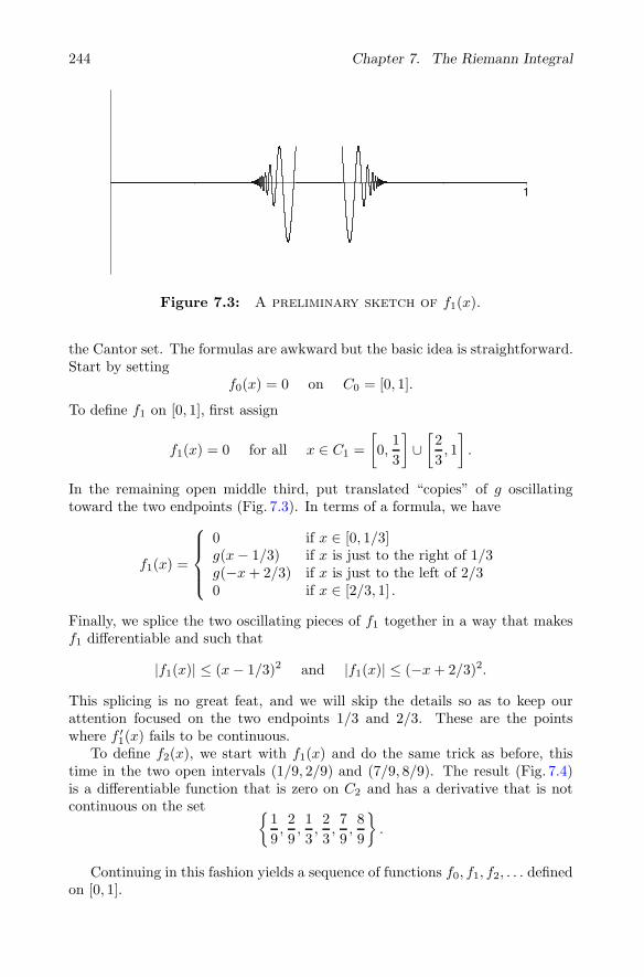
244 Chapter 7. The Riemann Integral
1
Figure 7.3: A preliminary sketch of f1(x).
the Cantor set. The formulas are awkward but the basic idea is straightforward.Start by setting
f0(x) = 0 on C0 = [0, 1].
To define f1 on [0, 1], first assign
f1(x) = 0 for all x ∈ C1 =
[
0,1
3
]
∪[2
3, 1
]
.
In the remaining open middle third, put translated “copies” of g oscillatingtoward the two endpoints (Fig. 7.3). In terms of a formula, we have
f1(x) =
⎧⎪⎪⎨
⎪⎪⎩
0 if x ∈ [0, 1/3]g(x− 1/3) if x is just to the right of 1/3g(−x+ 2/3) if x is just to the left of 2/30 if x ∈ [2/3, 1] .
Finally, we splice the two oscillating pieces of f1 together in a way that makesf1 differentiable and such that
|f1(x)| ≤ (x− 1/3)2 and |f1(x)| ≤ (−x+ 2/3)2.
This splicing is no great feat, and we will skip the details so as to keep ourattention focused on the two endpoints 1/3 and 2/3. These are the pointswhere f ′
1(x) fails to be continuous.To define f2(x), we start with f1(x) and do the same trick as before, this
time in the two open intervals (1/9, 2/9) and (7/9, 8/9). The result (Fig. 7.4)is a differentiable function that is zero on C2 and has a derivative that is notcontinuous on the set {
1
9,2
9,1
3,2
3,7
9,8
9
}
.
Continuing in this fashion yields a sequence of functions f0, f1, f2, . . . definedon [0, 1].

7.6. Lebesgue’s Criterion for Riemann Integrability 245
1
Figure 7.4: A graph of f2(x).
Exercise 7.6.15. (a) If c ∈ C, what is limn→∞ fn(c)?
(b) Why does limn→∞ fn(x) exist for x /∈ C?
Now, setf(x) = lim
n→∞ fn(x).
Exercise 7.6.16. (a) Explain why f ′(x) exists for all x /∈ C.
(b) If c ∈ C, argue that |f(x)| ≤ (x − c)2 for all x ∈ [0, 1]. Show how thisimplies f ′(c) = 0.
(c) Give a careful argument for why f ′(x) fails to be continuous on C. Re-member that C contains many points besides the endpoints of the intervalsthat make up C1, C2, C3, . . . .
Let’s take inventory of the situation. Our goal is to create a nonintegrablederivative. Our function f(x) is differentiable, and f ′ fails to be continuous onC. We are not quite done.
Exercise 7.6.17. Why is f ′(x) Riemann-integrable on [0, 1]?
The reason the Cantor set has measure zero is that, at each stage, 2n−1 openintervals of length 1/3n are removed from Cn−1. The resulting sum
∞∑
n=1
2n−1
(1
3n
)
converges to one, which means that the approximating sets C1, C2, C3, . . . havetotal lengths tending to zero. Instead of removing open intervals of length 1/3n
at each stage, let’s see what happens when we remove intervals of length 1/3n+1.
Exercise 7.6.18. Show that, under these circumstances, the sum of the lengthsof the intervals making up each Cn no longer tends to zero as n → ∞. What isthis limit?

246 Chapter 7. The Riemann Integral
1
Figure 7.5: A differentiable function with a non-integrable
derivative.
If we again take the intersection⋂∞
n=0 Cn, the result is a Cantor-type set withthe same topological properties—it is closed, compact, perfect, and containsno intervals. But a consequence of the previous exercise is that it no longerhas measure zero. This is just what we need to define our desired function.By repeating the preceding construction of f(x) on this new Cantor-type setof strictly positive measure, we get a differentiable function whose derivativehas too many points of discontinuity (Fig. 7.5). By Lebesgue’s Theorem, thisderivative cannot be integrated using the Riemann integral.
Exercise 7.6.19. As a final gesture, provide the example advertised in Exer-cise 7.6.13 of an integrable function f and a continuous function g where thecomposition f ◦ g is properly defined but not integrable. Exercise 4.3.12 maybe useful.
7.7 Epilogue
Riemann’s definition of the integral was a modification of Cauchy’s integral,which was originally designed for the purpose of integrating continuous func-tions. In this goal, the Riemann integral was a complete success. For continuousfunctions at least, the process of integration now stood on its own rigorous foot-ing, defined independently of differentiation. As analysis progressed, however,the dependence of integrability on continuity became problematic. The lastexample of Section 7.6 highlights one type of weakness: not every derivativecan be integrated. Another limitation of the Riemann integral arises in asso-ciation with limits of sequences of functions. To get a sense of this, let’s onceagain consider Dirichlet’s function g(x) introduced in Section 4.1. Recall thatg(x) = 1 whenever x is rational, and g(x) = 0 at every irrational point. Focusingon the interval [0, 1] for a moment, let
{r1, r2, r3, r4 . . .}

7.7. Epilogue 247
be an enumeration of the countable number of rational points in this interval.Now, let g1(x) = 1 if x = r1 and define g1(x) = 0 otherwise. Next, defineg2(x) = 1 if x is either r1 or r2, and let g2(x) = 0 at all other points. In general,for each n ∈ N, define
gn(x) =
{1 if x ∈ {r1, r2, . . . , rn}0 otherwise.
Notice that each gn has only a finite number of discontinuities and so is Riemann-
integrable with∫ 1
0 gn = 0. But we also have gn → g pointwise on theinterval [0, 1]. The problem arises when we remember that Dirichlet’s nowhere-continuous function is not Riemann-integrable. Thus, the equation
(1) limn→∞
∫ 1
0
gn =
∫ 1
0
g
fails to hold, not because the values on each side of the equal sign are differentbut because the value on the right-hand side does not exist. The content of The-orem 7.4.4 is that this equation does hold whenever we have gn → g uniformly.This is a reasonable way to resolve the situation, but it is a bit unsatisfyingbecause the deficiency in this case is not entirely with the type of convergencebut lies in the strength of the Riemann integral. If we could make sense of theright-hand side via some other definition of integration, then maybe equation(1) would actually be true.
Such a definition was introduced by Henri Lebesque in 1901. Generallyspeaking, Lebesgue’s integral is constructed using a generalization of lengthcalled the measure of a set. In the previous section, we studied sets of measurezero. In particular, we showed that the rational numbers in [0,1] (because theyare countable) have measure zero. The irrational numbers in [0,1] have measureone. This should not be too surprising because we now have that the measuresof these two disjoint sets add up to the length of the interval [0, 1]. Ratherthan chopping up the x-axis to approximate the area under the curve, Lebesguesuggested partitioning the y-axis. In the case of Dirichlet’s function g, thereare only two range values—zero and one. The integral, according to Lebesgue,could be defined via
∫ 1
0
g = 1 · [measure of set where g = 1] + 0 · [measure of set where g = 0]
= 1 · 0 + 0 · 1 = 0.
With this interpretation of∫ 1
0 g, equation (1) is now valid!The Lebesgue integral is presently the standard integral in advanced math-
ematics. The theory is taught to all graduate students, as well as to manyundergraduates, and it is the integral used in most research papers where inte-gration is required. The Lebesgue integral generalizes the Riemann integral inthe sense that any function that is Riemann-integrable is Lebesgue-integrableand integrates to the same value. The real strength of the Lebesgue integral

248 Chapter 7. The Riemann Integral
is that the class of integrable functions is much larger. Most importantly, thisclass includes the limits of different types of Cauchy sequences of integrablefunctions. This leads to a group of extremely important convergence theoremsrelated to equation (1) with hypotheses much weaker than the uniform conver-gence assumed in Theorem 7.4.4.
Despite its prevalence, the Lebesgue integral does have a few drawbacks.There are functions whose improper Riemann integrals exist but that are notLebesgue-integrable. Another disappointment arises from the relationship be-tween integration and differentiation. Even with the Lebesgue integral, it is stillnot possible to prove
∫ b
a
f ′ = f(b)− f(a)
without some additional assumptions on f . Around 1960, a new integral wasproposed that can integrate a larger class of functions than either the Riemannintegral or the Lebesgue integral and suffers from neither of the precedingweaknesses. Remarkably, this integral is actually a return to Riemann’s orig-inal technique for defining integration, with some small modifications in howwe describe the “fineness” of the partitions. An introduction to the generalizedRiemann integral is the topic of Section 8.1.

Chapter 8
Additional Topics
The foundation in analysis provided by the first seven chapters is sufficientbackground for the exploration of some advanced and historically importanttopics. The writing in this chapter is similar to that in the concluding projectsections of each individual chapter. Exercises are included within the expositionand are designed to make each section a narrative investigation into a significantachievement in the field of analysis.
8.1 The Generalized Riemann Integral
Chapter 7 concluded with Henri Lebesgue’s elegant result that a bounded func-tion is Riemann-integrable if and only if its points of discontinuity form a setof measure zero. To eliminate the dependence of integrability on continuity,Lebesgue proposed a new method of integration that has become the standardintegral in mathematics. In the Epilogue to Chapter 7, we briefly outlined someof the strengths and weaknesses of the Lebesgue integral, concluding with a lookback to the Fundamental Theorem of Calculus (Theorem 7.5.1). (Lebesgue’smeasure-zero criterion is not a prerequisite for understanding the material inthis section, but the discussion in Section 7.7 provides some useful context forwhat follows.)
If F is a differentiable function on [a, b], then in a perfect world we mighthope to prove that
(1)
∫ b
a
F ′ = F (b)− F (a).
Notice that although this is the conclusion of part (i) of Theorem 7.5.1, therewe needed the additional requirement that F ′ be Riemann-integrable. To drivethis point home, Section 7.6 concluded with an example of a function that has
© Springer Science+Business Media New York 2015S. Abbott, Understanding Analysis, Undergraduate Textsin Mathematics, DOI 10.1007/978-1-4939-2712-8 8
249

250 Chapter 8. Additional Topics
a derivative that the Riemann integral cannot handle. The Lebesgue integralalluded to earlier is a significant improvement. It can integrate our examplefrom Section 7.6, but ultimately it too suffers from the same setback. Not everyderivative is integrable, no matter which integral is used.
What follows is a short introduction to the generalized Riemann integral, dis-covered independently around 1960 by Jaroslav Kurzweil and Ralph Henstock.As mentioned in Section 7.7, this lesser-known modification of the Riemannintegral can actually integrate a larger class of functions than Lebesgue’s ubiq-uitous integral and yields a surprisingly simple proof of equation (1) above withno additional hypotheses.
The Riemann Integral as a Limit
Let
P = {x0, x1, x2, . . . , xn}be a partition of [a, b]. A tagged partition is one where in addition to P we havechosen points ck in each of the subintervals [xk−1, xk]. This sets the stage forthe concept of a Riemann sum. Given a function f : [a, b] → R, and a taggedpartition (P, {ck}nk=1), the Riemann sum generated by this partition is given by
R(f, P ) =
n∑
k=1
f(ck)(xk − xk−1).
Looking back at the definition of the upper sum
U(f, P ) =
n∑
k=1
Mk(xk − xk−1) where Mk = sup{f(x) : x ∈ [xk−1, xk]},
and the lower sum
L(f, P ) =
n∑
k=1
mk(xk − xk−1) where mk = inf{f(x) : x ∈ [xk−1, xk]},
it should be clear that
L(f, P ) ≤ R(f, P ) ≤ U(f, P )
for any bounded function f . In Definition 7.2.7, we characterized integrabilityby insisting that the infimum of the upper sums equal the supremum of thelower sums. Any Riemann sum is going to fall between a particular upper andlower sum. If the upper and lower sums are converging to some common value,then the Riemann sums are also eventually close to this value as well. The nexttheorem shows that it is possible to characterize Riemann integrability in a wayequivalent to Definition 7.2.7 using an ε–δ-type definition applied to Riemannsums.

8.1. The Generalized Riemann Integral 251
Definition 8.1.1. Let δ > 0. A partition P is δ-fine if every subinterval[xk−1, xk] satisfies xk − xk−1 < δ. In other words, every subinterval has widthless than δ.
Theorem 8.1.2 (Limit Criterion for Riemann Integrability). A boundedfunction f : [a, b] → R is Riemann-integrable with
∫ b
a
f = A
if and only if, for every ε > 0, there exists a δ > 0 such that, for any taggedpartition (P, {ck}) that is δ-fine, it follows that
|R(f, P )−A| < ε.
Before attempting the proof, we should point out that, in some treatments,the criterion in Theorem 8.1.2 is actually taken as the definition of Riemann inte-grability. In fact, this is how Riemann originally defined the concept. The spiritof this theorem is close to what is taught in most introductory calculus courses.To approximate the area under the curve, Riemann sums are constructed. Thehope is that as the partitions become finer, the corresponding approximationsget closer to the value of the integral. The content of Theorem 8.1.2 is thatif the function is integrable, then these approximations do indeed converge tothe value of the integral, regardless of how the tags are chosen. Conversely, ifthe approximating Riemann sums for finer and finer partitions collect aroundsome value A, then the function is integrable and integrates to A.
Proof. (⇒) For the forward direction, we begin with the assumption that f isintegrable on [a, b]. Given an ε > 0, we must produce a δ > 0 such that if
(P, {ck}) is any tagged partition that is δ-fine, then |R(f, P )− ∫ b
a f | < ε.Because f is integrable, we know there exists a partition Pε such that
U(f, Pε)− L(f, Pε) <ε
3.
Let M > 0 be a bound on |f |, and let n be the number of subintervals of Pε (sothat Pε really consists of n+ 1 points in [a, b]). We will argue that choosing
δ = ε/9nM
has the desired property.Here is the idea. Let (P, {ck}) be an arbitrary tagged partition of [a, b] that
is δ-fine, and let P ′ = P ∪ Pε. The key is to establish the string of inequalities
L(f, P ′)− ε
3< L(f, P ) ≤ U(f, P ) < U(f, P ′) +
ε
3.
Exercise 8.1.1. (a) Explain why both the Riemann sum R(f, P ) and∫ b
a ffall between L(f, P ) and U(f, P ).

252 Chapter 8. Additional Topics
(b) Explain why U(f, P ′)− L(f, P ′) < ε/3.
By the previous exercise, if we can show U(f, P ) < U(f, P ′) + ε/3 (andsimilarly L(f, P ′)− ε/3 < L(f, P )), then it will follow that
∣∣∣∣∣R(f, P )−
∫ b
a
f
∣∣∣∣∣< ε
and the proof will be done. Thus, we turn our attention toward estimating thedistance between U(f, P ) and U(f, P ′).
Exercise 8.1.2. Explain why U(f, P )− U(f, P ′) ≥ 0.
A typical term in either U(f, P ) or U(f, P ′) has the form Mk(xk − xk−1),where Mk is the supremum of f over [xk−1, xk]. A good number of these termsappear in both upper sums and so cancel out.
Exercise 8.1.3. (a) In terms of n, what is the largest number of terms of theform Mk(xk − xk−1) that could appear in one of U(f, P ) or U(f, P ′) butnot the other?
(b) Finish the proof in this direction by arguing that
U(f, P )− U(f, P ′) < ε/3.
(⇐) For this direction, we assume that the ε–δ criterion in Theorem 8.1.2holds and argue that f is integrable. Integrability, as we have defined it, dependson our ability to choose partitions for which the upper sums are close to thelower sums. We have remarked that given any partition P , it is always the casethat
L(f, P ) ≤ R(f, P ) ≤ U(f, P )
no matter which tags are chosen to compute R(f, P ).
Exercise 8.1.4. (a) Show that if f is continuous, then it is possible to picktags {ck}nk=1 so that
R(f, P ) = U(f, P ).
Similarly, there are tags for which R(f, P ) = L(f, P ) as well.
(b) If f is not continuous, it may not be possible to find tags for whichR(f, P ) = U(f, P ). Show, however, that given an arbitrary ε > 0, itis possible to pick tags for P so that
U(f, P )−R(f, P ) < ε.
The analogous statement holds for lower sums.
Exercise 8.1.5. Use the results of the previous exercise to finish the proof ofTheorem 8.1.2.

8.1. The Generalized Riemann Integral 253
Gauges and δ(x)-fine Partitions
The key to the generalized Riemann integral is to allow the δ in Theorem 8.1.2to be a function of x.
Definition 8.1.3. A function δ : [a, b] → R is called a gauge on [a, b] if δ(x) > 0for all x ∈ [a, b].
Definition 8.1.4. Given a particular gauge δ(x), a tagged partition (P, {ck}nk=1)is δ(x)-fine if every subinterval [xk−1, xk] satisfies xk − xk−1 < δ(ck). In otherwords, each subinterval [xk−1, xk] has width less than δ(ck).
It is important to see that if δ(x) is a constant function, then Definition 8.1.4says precisely the same thing as Definition 8.1.1. In the case where δ(x) is not aconstant, Definition 8.1.4 describes a way of measuring the fineness of partitionsthat is quite different.
Exercise 8.1.6. Consider the interval [0, 1].
(a) If δ(x) = 1/9, find a δ(x)-fine tagged partition of [0, 1]. Does the choiceof tags matter in this case?
(b) Let
δ(x) =
{1/4 if x = 0x/3 if 0 < x ≤ 1.
Construct a δ(x)-fine tagged partition of [0,1].
The tinkering required in Exercise 8.1.6 (b) may cast doubt on whetheran arbitrary gauge always admits a δ(x)-fine partition. However, it is not toodifficult to show that this is indeed the case.
Theorem 8.1.5. Given a gauge δ(x) on an interval [a, b], there exists a taggedpartition (P, {ck}nk=1) that is δ(x)-fine.
Proof. Let I0 = [a, b]. It may be possible to find a tag such that the trivialpartition P = {a, b} works. Specifically, if b− a < δ(x) for some x ∈ [a, b], thenwe can set c1 equal to such an x and notice that (P, {c1}) is δ(x)-fine. If nosuch x exists, then bisect [a, b] into two equal halves.
Exercise 8.1.7. Finish the proof of Theorem 8.1.5.
Generalized Riemann Integrability
Keeping in mind that Theorem 8.1.2 offers an equivalent way to define Riemannintegrability, we now propose a new method for defining the value of the integral.

254 Chapter 8. Additional Topics
Definition 8.1.6. A function f on [a, b] has generalized Riemann integral Aif, for every ε > 0, there exists a gauge δ(x) on [a, b] such that for each taggedpartition (P, {ck}nk=1) that is δ(x)-fine, it is true that
|R(f, P )−A| < ε.
In this case, we write A =∫ b
a f .
Theorem 8.1.7. If a function has a generalized Riemann integral, then thevalue of the integral is unique.
Proof. Assume that a function f has generalized Riemann integral A1 and thatit also has generalized Riemann integral A2. We must prove A1 = A2.
Exercise 8.1.8. Finish the argument.
The implications of Definition 8.1.6 on the resulting class of integrable func-tions are far reaching. This is somewhat surprising given that the criteria forintegrability in Definition 8.1.6 and Theorem 8.1.2 differ in such a small way.One observation that should be immediately evident is the following.
Exercise 8.1.9. Explain why every function that is Riemann-integrable with∫ b
af = A must also have generalized Riemann integral A.
The converse statement is not true, and that is the important point. Oneexample that we have of a non-Riemann-integrable function is Dirichlet’s func-tion
g(x) =
{1 if x ∈ Q0 if x /∈ Q
which has discontinuities at every point of R.
Theorem 8.1.8. Dirichlet’s function g(x) is generalized Riemann-integrable on
[0, 1] with∫ 1
0 g = 0.
Proof. Let ε > 0. By Definition 8.1.6, we must construct a gauge δ(x) on [0, 1]such that whenever (P, {ck}nk=1) is a δ(x)-fine tagged partition, it follows that
0 ≤n∑
k=1
g(ck)(xk − xk−1) < ε.
The gauge represents a restriction on the size of Δxk = xk − xk−1 in the sensethat Δxk < δ(ck). The Riemann sum consists of products of the form g(ck)Δxk.Thus, for irrational tags, there is nothing to worry about because g(ck) = 0 inthis case. Our task is to make sure that any time a tag ck is rational, it comesfrom a suitably thin subinterval.
Let {r1, r2, r3, . . .} be an enumeration of the countable set of rational num-bers contained in [0, 1]. For each rk, set δ(rk) = ε/2k+1. For x irrational, setδ(x) = 1.

8.1. The Generalized Riemann Integral 255
Exercise 8.1.10. Show that if (P, {ck}nk=1) is a δ(x)-fine tagged partition, thenR(g, P ) < ε.
Dirichlet’s function fails to be Riemann-integrable because, given any (un-tagged) partition, it is possible to make R(g, P ) = 1 or R(g, P ) = 0 by choosingthe tags to be either all rational or all irrational. For the generalized Rie-mann integral, choosing all rational tags results in a tagged partition that isnot δ(x)-fine (when δ(x) is small on rational points) and so does not have to beconsidered. In general, allowing for nonconstant gauges allows us to be morediscriminating about which tagged partitions qualify as δ(x)-fine. The result,as we have just seen, is that it may be easier to achieve the inequality
|R(f, P )−A| < ε
for the often smaller and more carefully selected set of tagged partitions thatremain.
The Fundamental Theorem of Calculus
We conclude this brief introduction to the generalized Riemann integral with aproof of the Fundamental Theorem of Calculus. As was alluded to earlier, themost notable distinction between the following theorem and part (i) of Theorem7.5.1 is that here we do not need to assume that the derivative function is inte-grable. Using the generalized Riemann integral, every derivative is integrable,and the integral can be evaluated using the antiderivative in the familiar way.It is also interesting to note that in Theorem 7.5.1 the Mean Value Theoremplayed the crucial role in the argument, but it is not needed here.
Theorem 8.1.9. Assume F : [a, b] → R is differentiable at each point in [a, b]and set f(x) = F ′(x). Then, f has the generalized Riemann integral
∫ b
a
f = F (b)− F (a).
Proof. Let P = {x0, x1, x2, . . . , xn} be a partition of [a, b]. Both this proof andthe proof of Theorem 7.5.1 make use of the following fact.
Exercise 8.1.11. Show that
F (b)− F (a) =
n∑
k=1
[F (xk)− F (xk−1)] .

256 Chapter 8. Additional Topics
If {ck}nk=1 is a set of tags for P , then we can estimate the difference betweenthe Riemann sum R(f, P ) and F (b)− F (a) by
|F (b)− F (a)−R(f, P )| =
∣∣∣∣∣
n∑
k=1
[F (xk)− F (xk−1)− f(ck)(xk − xk−1)]
∣∣∣∣∣
≤n∑
k=1
|F (xk)− F (xk−1)− f(ck)(xk − xk−1)| .
Let ε > 0. To prove the theorem, we must construct a gauge δ(c) such that
(2) |F (b)− F (a)−R(f, P )| < ε
for all (P, {ck}) that are δ(c)-fine. (Using the variable c in the gauge functionis more convenient than x in this case.)
Exercise 8.1.12. For each c ∈ [a, b], explain why there exists a δ(c) > 0 (aδ > 0 depending on c) such that
∣∣∣∣F (x)− F (c)
x− c− f(c)
∣∣∣∣ < ε
for all 0 < |x− c| < δ(c).
This δ(c) is the desired gauge on [a, b]. Let (P, {ck}nk=1) be a δ(c)-fine parti-tion of [a, b]. It just remains to show that equation (2) is satisfied for this taggedpartition.
Exercise 8.1.13. (a) For a particular ck ∈ [xk−1, xk] of P , show that
|F (xk)− F (ck)− f(ck)(xk − ck)| < ε(xk − ck)
and|F (ck)− F (xk−1)− f(ck)(ck − xk−1)| < ε(ck − xk−1).
(b) Now, argue that
|F (xk)− F (xk−1)− f(ck)(xk − xk−1)| < ε(xk − xk−1),
and use this fact to complete the proof of the theorem.
If we consider the function
F (x) =
{x3/2 sin(1/x) if x �= 00 if x = 0
then it is not too difficult to show that F is differentiable everywhere, includingx = 0, with
F ′(x) ={
(3/2)√x sin(1/x)− (1/
√x) cos(1/x) if x �= 0
0 if x = 0.

8.1. The Generalized Riemann Integral 257
What is notable here is that the derivative is unbounded near the origin. Thetheory of the ordinary Riemann integral begins with the assumption that weonly consider bounded functions on closed intervals, but there is no such re-striction for the generalized Riemann integral. Theorem 8.1.9 proves that F ′
has a generalized integral. Now, improper Riemann integrals have been createdto extend Riemann integration to some unbounded functions, but it is anotherinteresting fact about the generalized Riemann integral that any function hav-ing an improper integral must already be integrable in the sense described inDefinition 8.1.6.
As a parting gesture, let’s show how Theorem 8.1.9 yields a short verificationof the substitution technique from calculus.
Theorem 8.1.10 (Change-of-variable Formula). Let g : [a, b] → R bedifferentiable at each point of [a, b], and assume F is differentiable on the setg([a, b]). If f(x) = F ′(x) for all x ∈ g([a, b]), then
∫ b
a
(f ◦ g) · g′ =∫ g(b)
g(a)
f.
Proof. The hypothesis of the theorem guarantees that the function (F ◦ g)(x)is differentiable for all x ∈ [a, b].
Exercise 8.1.14. (a) Why are we sure that f and (F ◦ g)′ have generalizedRiemann integrals?
(b) Use Theorem 8.1.9 to finish the proof.
The impressive properties of the generalized Riemann integral do not endhere. The central source for the material in this section is Robert Bartle’saward winning article “Return to the Riemann Integral,” which appeared in theAmerican Mathematical Monthly, October, 1996. The article goes on to discussconvergence theorems for this new integral in the spirit of Theorem 7.4.4, andoutlines the argument that the collection of integrable functions is strictly largerwhen the Lebesgue integral is replaced by the generalized Riemann integral. Inlight of this, the author boldly declares that“the time has come to discard theLebesgue integral as the primary integral.” (Italics in the original.)
That this revolution has not come to pass may simply be due to a case ofoverwhelming inertia, but a contributing factor is very likely the geometricallysatisfying intuition of Lebesgue’s theory. At the heart of Lebesgue’s approach tointegration is the desire to generalize the concepts of length and area. Althoughone can certainly use a properly developed integral to give a rigorous definitionfor the length—or measure—of a general set, there is a compelling argumentthat this puts the ideas in the wrong pedagogical order. Rather than using asophisticated integral to generalize a primitive notion such as length, Lebesguefound an effective way to talk about the length of a very wide class of sets, andused that to build his definition of the integral. The very elegant result of hisendeavor is likely to be the industry standard for a long time to come.

258 Chapter 8. Additional Topics
8.2 Metric Spaces and the Baire Category
Theorem
A natural question to ask is whether the theorems we have proved about se-quences, series, and functions in R have analogues in the plane R2 or in evenhigher dimensions. Looking back over the proofs, one crucial observation isthat most of the arguments depend on just a few basic properties of the abso-lute value function. Interpreting the statement “|x− y|” to mean the “distancefrom x to y in R,” our aim is to experiment with other ways of measuring dis-tance on other sets such as R2 and C[0, 1], the space of continuous functions on[0, 1].
Definition 8.2.1. Given a set X , a function d : X ×X → R is a metric on Xif for all x, y ∈ X :
(i) d(x, y) ≥ 0 with d(x, y) = 0 if and only if x = y,
(ii) d(x, y) = d(y, x), and
(iii) for all z ∈ X , d(x, y) ≤ d(x, z) + d(z, y).
A metric space is a set X together with a metric d.
Property (iii) in the previous definition is the “triangle inequality.” The nexttwo exercises illustrate the point that the same set X can be home to severaldifferent metrics. When referring to a metric space, we must specify the set andthe particular distance function d.
Exercise 8.2.1. Decide which of the following are metrics on X = R2. Foreach, we let x = (x1, x2) and y = (y1, y2) be points in the plane.
(a) d(x, y) =√(x1 − y1)2 + (x2 − y2)2.
(b) d(x, y) = max{|x1 − y1|, |x2 − y2|}.(c) d(x, y) = |x1x2 + y1y2|.The metric in part (a) of the previous exercise is the familiar Euclidean
distance between two points in the plane. This is often referred to as the “usual”or “standard” metric on R2. The usual metric on R is our old friend d(x, y) =|x− y|.Exercise 8.2.2. Let C[0, 1] be the collection of continuous functions on theclosed interval [0, 1]. Decide which of the following are metrics on C[0, 1].
(a) d(f, g) = sup{|f(x)− g(x)| : x ∈ [0, 1]}.(b) d(f, g) = |f(1)− g(1)|.
(c) d(f, g) =∫ 1
0 |f − g|.

8.2. Metric Spaces and the Baire Category Theorem 259
The following distance function is called the discrete metric and can bedefined on any set X . For any x, y ∈ X , let
ρ(x, y) =
{1 if x �= y0 if x = y.
Exercise 8.2.3. Verify that the discrete metric is actually a metric.
Basic Definitions
Definition 8.2.2. Let (X, d) be a metric space. A sequence (xn) ⊆ X convergesto an element x ∈ X if for all ε > 0 there exists an N ∈ N such that d(xn, x) < εwhenever n ≥ N .
Definition 8.2.3. A sequence (xn) in a metric space (X, d) is a Cauchy sequenceif for all ε > 0 there exists an N ∈ N such that d(xm, xn) < ε wheneverm,n ≥ N .
Exercise 8.2.4. Show that a convergent sequence is Cauchy.
The Cauchy Criterion, as it is called in R, was an “if and only if” statement.In the general metric space setting, however, the converse statement does notalways hold. Recall that, in R, the assertion that “Cauchy sequences converge”was shown to be equivalent to the Axiom of Completeness. In order to transportthe Axiom of Completeness into a metric space, we would need to have anordering on our space so that we could discuss such things as upper bounds. Itis an interesting observation that not every set can be ordered in a satisfyingway (the points in R2 for example). Even without an ordering, we are still goingto want completeness. For metric spaces, the convergence of Cauchy sequencesis taken to be the definition of completeness.
Definition 8.2.4. A metric space (X, d) is complete if every Cauchy sequencein X converges to an element of X .
Exercise 8.2.5. (a) Consider R2 with the discrete metric ρ(x, y) examinedin Exercise 8.2.3. What do Cauchy sequences look like in this space? IsR2 complete with respect to this metric?
(b) Show that C[0, 1] is complete with respect to the metric in Exercise8.2.2 (a).
(c) Define C1[0, 1] to be the collection of differentiable functions on [0,1] whosederivatives are also continuous. Is C1[0, 1] complete with respect to themetric defined in Exercise 8.2.2 (a)?
Because completeness is a prerequisite for doing anything significant in theway of analysis, the metric in Exercise 8.2.2 (a) is the most natural metric toconsider when working with C[0, 1]. The notation
‖f − g‖∞ = d(f, g) = sup{|f(x)− g(x)| : x ∈ [0, 1]}

260 Chapter 8. Additional Topics
is standard, and setting g = 0 gives the so-called “sup norm”
‖f‖∞ = d(f, 0) = sup{|f(x)| : x ∈ [0, 1]}.
In all upcoming discussions, it is assumed that the space C[0, 1] is endowed withthis metric unless otherwise specified.
Definition 8.2.5. Let (X, d1) and (Y, d2) be metric spaces. A function f :X → Y is continuous at x ∈ X if for all ε > 0 there exists a δ > 0 such thatd2(f(x), f(y)) < ε whenever d1(x, y) < δ.
Exercise 8.2.6. Which of these functions from C[0, 1] to R (with the usualmetric) are continuous?
(a) g(f) =∫ 1
0fk, where k is some fixed function in C[0, 1].
(b) g(f) = f(1/2).
(c) g(f) = f(1/2), but this time with respect to the metric on C[0, 1] fromExercise 8.2.2 (c).
Topology on Metric Spaces
Definition 8.2.6. Given ε > 0 and an element x in the metric space (X, d),the ε-neighborhood of x is the set Vε(x) = {y ∈ X : d(x, y) < ε}.Exercise 8.2.7. Describe the ε-neighborhoods in R2 for each of the differentmetrics described in Exercise 8.2.1. How about for the discrete metric?
With the definition of an ε-neighborhood, we can now define open sets , limitpoints , and closed sets exactly as we did before. A set O ⊆ X is open if forevery x ∈ O we can find a neighborhood Vε(x) ⊆ O. A point x is a limit pointof a set A if every Vε(x) intersects A in some point other than x. A set C isclosed if it contains its limit points.
Exercise 8.2.8. Let (X, d) be a metric space.
(a) Verify that a typical ε-neighborhood Vε(x) is an open set. Is the set
Cε(x) = {y ∈ X : d(x, y) ≤ ε}
a closed set?
(b) Show that a set E ⊆ X is open if and only if its complement is closed.
Exercise 8.2.9. (a) Show that the set Y = {f ∈ C[0, 1] : ‖f‖∞ ≤ 1} isclosed in C[0, 1].
(b) Is the set T = {f ∈ C[0, 1] : f(0) = 0} open, closed, or neither in C[0, 1]?
We define compactness in metric spaces just as we did for R.

8.2. Metric Spaces and the Baire Category Theorem 261
Definition 8.2.7. A subset K of a metric space (X, d) is compact if everysequence in K has a convergent subsequence that converges to a limit in K.
An extremely useful characterization of compactness in R is the propositionthat a set is compact if and only if it is closed and bounded. For abstract metricspaces, this proposition only holds in the forward direction.
Exercise 8.2.10. (a) Supply a definition for bounded subsets of a metricspace (X, d).
(b) Show that if K is a compact subset of the metric space (X, d), then K isclosed and bounded.
(c) Show that Y ⊆ C[0, 1] from Exercise 8.2.9 (a) is closed and bounded butnot compact.
A good hint for part (c) of the previous exercise can be found in Exer-cise 6.2.14 from Chapter 6. This exercise defines the concept of an equicontin-uous family of functions, which is a key ingredient in the Arzela–Ascoli The-orem (Exercise 6.2.15). The Arzela–Ascoli Theorem states that any bounded,equicontinuous collection of functions in C[0, 1] must have a uniformly conver-gent subsequence. One way to summarize this famous result—which we did nothave the language for in Chapter 6—is as a statement describing a particularclass of compact subsets in C[0, 1]. Looking at the definition of compactness,and remembering that the uniform limit of continuous functions is continuous,the Arzela–Ascoli Theorem states that any closed, bounded, equicontinuouscollection of functions is a compact subset of C[0, 1].
Definition 8.2.8. Given a subset E of a metric space (X, d), the closure E isthe union of E together with its limit points. The interior of E is denoted byE◦ and is defined as
E◦ = {x ∈ E : there exists Vε(x) ⊆ E}.Closure and interior are dual concepts. Results about these concepts come
in pairs and exhibit an elegant and useful symmetry.
Exercise 8.2.11. (a) Show that E is closed if and only if E = E. Show thatE is open if and only if E◦ = E.
(b) Show that Ec= (Ec)◦, and similarly that (E◦)c = Ec.
A good hint for this exercise is to review the proofs from Chapter 3, whereclosure at least is discussed. Thinking of all of these concepts as they relateto R or R2 with the usual metric is not a bad idea. However, it is importantto remember also that rigorous proofs must be constructed purely from therelevant definitions.
Exercise 8.2.12. (a) Show
Vε(x) ⊆ {y ∈ X : d(x, y) ≤ ε},in an arbitrary metric space (X, d).
262 Chapter 8. Additional Topics
(b) To keep things from sounding too familiar, find an example of a specificmetric space where
Vε(x) �= {y ∈ X : d(x, y) ≤ ε}.We are on our way toward the Baire Category Theorem. The next definitions
provide the final bit of vocabulary needed to state the result.
Definition 8.2.9. A set A ⊆ X is dense in the metric space (X, d) if A = X .
A subset E of a metric space (X, d) is nowhere-dense in X if E◦is empty.
Exercise 8.2.13. If E is a subset of a metric space (X, d), show that E isnowhere-dense in X if and only if E
cis dense in X .
The Baire Category Theorem
In Section 3.5, we proved Baire’s Theorem, which states that it is impossible towrite the real numbersR as the countable union of nowhere-dense sets. Previousto this, we knew thatR was too big to be written as the countable union of singlepoints (R is uncountable), but Baire’s Theorem improves on this by assertingthat the only way to make R from a countable union of arbitrary sets is forthe closure of at least one of these sets to contain an interval. The keystoneto the proof of Baire’s Theorem is the completeness of R. The idea now is toreplace R with an arbitrary complete metric space and prove the theorem inthis more general setting. This leads to a statement that can be used to discussthe size and structure of other spaces such as R2 and C[0, 1]. At the end ofChapter 3, we mentioned one particularly fascinating implication of this resultfor C[0, 1], which is that—despite the substantial difficulty required to producean example of one—most continuous functions are nowhere-differentiable. Itwould be a good idea at this point to reread Sections 3.6 and 5.5. We are nowequipped to carry out the details promised in these discussions.
Theorem 8.2.10. Let (X, d) be a complete metric space, and let {On} be acountable collection of dense, open subsets of X. Then,
⋂∞n=1 On is not empty.
Proof. When we proved this theorem on R, completeness manifested itself inthe form of the Nested Interval Property. We could derive something akinto NIP in the metric space setting, but instead let’s take an approach thatuses the convergence of Cauchy sequences (because this is how we have definedcompleteness).
Pick x1 ∈ O1. Because O1 is open, there exists an ε1 > 0 such thatVε1(x1) ⊆ O1.
Exercise 8.2.14. (a) Give the details for why we know there exists a pointx2 ∈ Vε1(x1)∩O2 and an ε2 > 0 satisfying ε2 < ε1/2 with Vε2(x2) containedin O2 and
Vε2(x2) ⊆ Vε1(x1).

8.2. Metric Spaces and the Baire Category Theorem 263
(b) Proceed along this line and use the completeness of (X, d) to produce asingle point x ∈ On for every n ∈ N.
Theorem 8.2.11 (Baire Category Theorem). A complete metric space isnot the union of a countable collection of nowhere-dense sets.
Exercise 8.2.15. Complete the proof of the theorem.
This result is called the Baire Category Theorem because it creates twocategories of size for subsets in a metric space. A set of “first category” is onethat can be written as a countable union of nowhere-dense sets. These are thesmall, intuitively thin subsets of a metric space. We now see that if our metricspace is complete, then it is necessarily of “second category,” meaning it cannotbe written as a countable union of nowhere-dense sets. Given a subset A of acomplete metric space X , showing that A is of first category is a mathematicallyprecise way of demonstrating that A constitutes a very minor portion of the setX . The term “meager” is often used to mean a set of first category.
With the stage set, we now outline the argument that continuous functionsthat are differentiable at even one point of [0,1] form a meager subset of themetric space C[0, 1].
Theorem 8.2.12. The set
D = {f ∈ C[0, 1] : f ′(x) exists for some x ∈ [0, 1]}
is a set of first category in C[0, 1].
Proof. For each pair of natural numbers m,n, define
Am,n =
{
f ∈ C[0, 1] : there exists x ∈ [0, 1] where
∣∣∣∣f(x)− f(t)
x− t
∣∣∣∣ ≤ n whenever 0 < |x− t| < 1
m
}
.
This definition takes some time to digest. Think of 1/m as defining a δ-neighborhood around the point x, and view n as an upper bound on the mag-nitude of the slopes of lines through the two points (x, f(x)) and (t, f(t)). Theset Am,n contains any function in C[0, 1] for which it is possible to find atleast one point x where the slopes through (x, f(x)) and points on the functionnearby—within 1/m to be precise—are bounded by n.
Exercise 8.2.16. Show that if f ∈ C[0, 1] is differentiable at a point x ∈ [0, 1],then f ∈ Am,n for some pair m,n ∈ N.
The collection of subsets {Am,n : m,n ∈ N} is countable, and we have justseen that the union of these sets contains our set D. Because it is not difficultto see that a subset of a set of first category is first category, the final hurdle inthe argument is to prove that each Am,n is nowhere-dense in C[0, 1].

264 Chapter 8. Additional Topics
Fix m and n. The first order of business is to prove that Am,n is a closedset. To this end, let (fk) be a sequence in Am,n and assume fk → f in C[0, 1].We need to show f ∈ Am,n.
Because fk ∈ Am,n, then for each k ∈ N there exists a point xk ∈ [0, 1]where ∣
∣∣∣fk(xk)− fk(t)
xk − t
∣∣∣∣ ≤ n for all 0 < |xk − t| < 1/m.
Exercise 8.2.17. (a) The sequence (xk) does not necessarily converge, butexplain why there exists a subsequence (xkl
) that is convergent. Let x =lim(xkl
).
(b) Prove that fkl(xkl
) → f(x).
(c) Now finish the proof that Am,n is closed.
Because Am,n is closed, Am,n = Am,n. In order to prove that Am,n isnowhere-dense, we just have to show that it contains no ε-neighborhoods, sopick an arbitrary f ∈ Am,n, let ε > 0, and consider the ε-neighborhood Vε(f)in C[0, 1]. To show that this set is not contained in Am,n, we must produce afunction g ∈ C[0, 1] that satisfies ‖f − g‖∞ < ε and has the property that thereis no point x ∈ [0, 1] where
∣∣∣∣g(x)− g(t)
x− t
∣∣∣∣ ≤ n for all 0 < |x− t| < 1/m.
Exercise 8.2.18. A continuous function is called polygonal if its graph consistsof a finite number of line segments.
(a) Show that there exists a polygonal function p ∈ C[0, 1] satisfying‖f − p‖∞ < ε/2.
(b) Show that if h is any function in C[0, 1] that is bounded by 1, then thefunction
g(x) = p(x) +ε
2h(x)
satisfies g ∈ Vε(f).
(c) Construct a polygonal function h(x) in C[0, 1] that is bounded by 1 andleads to the conclusion g /∈ Am,n, where g is defined as in (b). Explainhow this completes the argument for Theorem 8.2.12.
8.3 Euler’s Sum
In Section 6.1 we saw Euler’s first and most famous derivation of the formula
1 +1
4+
1
9+
1
16+
1
25+ · · · = π2
6.

8.3. Euler’s Sum 265
At the crux of this argument are two representations for the function sin(x).The first is the standard Taylor series representation
(1) sin(x) = x− x3
3!+
x5
5!− x7
7!+ · · · ,
and the second is an infinite product representation
(2) sin(x) = x(1− x
π
)(1 +
x
π
)(1− x
2π
)(1 +
x
2π
)· · · .
Although we have since made rigorous sense of the first equation (Example 6.6.4),proving the validity of equation (2) is still beyond our means.
The news is not all bad, however. In the time since Euler first made thisdiscovery, dozens of different proofs for this result have been published, start-ing with several by Euler himself and continuing right up to the present. Themachinery required in these arguments runs the gamut from multi-variable cal-culus to Fourier series to complex integration, but one in particular due to BooRim Choe relies mainly on Taylor series expansions and properties of uniformlyconvergent series. Choe’s argument was published in 1987 but actually has muchin common with one of Euler’s original attempts. The proof outlined in thissection follows Choe’s argument with some simplifications due to Peter Duren.1
Wallis’s Product
Even though we don’t currently have the tools to prove the infinite productformula for sin(x) in equation (2), we can prove a special case.
Exercise 8.3.1. Supply the details to show that when x = π/2 the productformula in (2) is equivalent to
(3)π
2= lim
n→∞
(2 · 21 · 3
)(4 · 43 · 5
)(6 · 65 · 7
)
· · ·(
2n · 2n(2n− 1)(2n+ 1)
)
,
where the infinite product in (2) is interpreted to be a limit of partial products.(Although it is not necessary for what follows, it might be useful to review thetreatment of infinite products in Exercises 2.4.10 and 2.7.10.)
The goal of the next few exercises is to supply a proper proof for equation (3).This curious formula involving π was first discovered by JohnWallis (1616–1703)and will provide some key ingredients for our proof of Euler’s sum. It resurfacesagain in Section 8.4 where the factorial function is defined.
Set
bn =
∫ π2
0
sinn(x)dx , for n = 0, 1, 2, . . . .
The first few terms are easy enough to calculate; in particular,
b0 =
∫ π2
0
1dx =π
2and b1 =
∫ π2
0
sin(x)dx = 1.
1[13], p. 92–95

266 Chapter 8. Additional Topics
Exercise 8.3.2. Assume h(x) and k(x) have continuous derivatives on [a, b]and derive the integration-by-parts formula
∫ b
a
h(t)k′(t)dt = h(b)k(b)− h(a)k(a)−∫ b
a
h′(t)k(t)dt .
Exercise 8.3.3. (a) Using the simple identity sinn(x) = sinn−1(x) sin(x) andthe previous exercise, derive the recurrence relation
bn =n− 1
nbn−2 for all n ≥ 2.
(b) Use this relation to generate the first three even terms and the first threeodd terms of the sequence (bn).
(c) Write a general expression for b2n and b2n+1.
Because 0 ≤ sinn+1(x) ≤ sinn(x) on [0, π/2], it follows that bn+1 ≤ bn and(bn) is decreasing. It turns out that (bn) → 0 but that isn’t the limit we areinterested in at the moment.
Exercise 8.3.4. Show
limn→∞
b2nb2n+1
= 1,
and use this fact to finish the proof of Wallis’s product formula in (3).
There are some standard techniques for working with the notation of equa-tion (3). For instance,
2 · 4 · 6 · · · (2n) = 2nn!
and
1 · 3 · 5 · · · (2n+ 1) =(2n+ 1)!
2 · 4 · 6 · · · (2n) =(2n+ 1)!
2nn!.
Exercise 8.3.5. Derive the following alternative form of Wallis’s product for-mula: √
π = limn→∞
22n(n!)2
(2n)!√n.
Taylor Series
The next step in the argument is to generate the Taylor series for arcsin(x). Thisis not really possible to do directly from Taylor’s formula for the coefficients,but keeping in mind that
(arcsin(x))′ =1√
1− x2,
we can get where we want to go by first finding the expansion for 1/√1− x.
8.3. Euler’s Sum 267
Exercise 8.3.6. Show that 1/√1− x has Taylor expansion
∑∞n=0 cnx
n, wherec0 = 1 and
cn =(2n)!
22n(n!)2=
1 · 3 · 5 · · · (2n− 1)
2 · 4 · 6 · · · 2nfor n ≥ 1.
The coefficients cn should look familiar from our work on Wallis’s product.Exercise 8.3.5 can be rephrased as
√π = lim
n→∞1
cn√n.
Exercise 8.3.7. Show that lim cn = 0 but∑∞
n=0 cn diverges.
The divergence of∑∞
n=0 cn makes sense when we consider the Taylor seriesfor 1/
√1− x. We want to determine the values of x for which
(4)1√1− x
=
∞∑
n=0
cnxn ,
and x = 1 is not in the domain of the left side. We do aim to prove (4) for allx ∈ (−1, 1) but the usual word of warning is in order. Having computed thecoefficients cn, it is not enough to simply argue that the series on the right sideconverges when |x| < 1. To properly establish (4) we are going to show thatthe error function
EN (x) =1√1− x
−N∑
n=0
cnxn
tends to zero as N → ∞. Back in Section 6.6, the primary tool we used for thistask was Lagrange’s Remainder Theorem (Theorem 6.6.3), but it is not up tothis particular challenge
Exercise 8.3.8. Using the expression for EN (x) from Lagrange’s RemainderTheorem, show that equation (4) is valid for all |x| < 1/2. What goes wrongwhen we try to use this method to prove (4) for x ∈ (1/2, 1)?
The Integral Form of the Remainder
The moral of the previous exercise is that we need a different method for es-timating EN (x). The Lagrange form of the remainder grows out of the MeanValue Theorems and yields a formula for the error function in terms of thederivative f (N+1). Now that we are in possession of a proper definition of theintegral, we can derive another useful formula for EN (x).
Theorem 8.3.1 (Integral Remainder Theorem). Let f be differentiableN + 1 times on (−R,R) and assume f (N+1) is continuous. Define an =f (n)(0)/n! for n = 0, 1, . . . , N , and let
SN (x) = a0 + a1x+ a2x2 + · · ·+ aNxN .

268 Chapter 8. Additional Topics
For all x ∈ (−R,R), the error function EN (x) = f(x)− SN (x) satisfies
EN (x) =1
N !
∫ x
0
f (N+1)(t)(x− t)Ndt .
Proof. The case x = 0 is easy to check, so let’s take x �= 0 in (−R,R) and keepin mind that x is a fixed constant in what follows. To avoid a few technicaldistractions, let’s just consider the case x > 0.
Exercise 8.3.9. (a) Show
f(x) = f(0) +
∫ x
0
f ′(t)dt .
(b) Now use a previous result from this section to show
f(x) = f(0) + f ′(0)x+
∫ x
0
f ′′(t)(x− t)dt .
(c) Continue in this fashion to complete the proof of the theorem.
To gain a better understanding of this formulation for EN (x) and simulta-neously make some headway on our exploration of equation (4), let’s return tothe special case f(x) = 1/
√1− x.
Exercise 8.3.10. (a) Make a rough sketch of 1/√1− x and S2(x) over the
interval (−1, 1), and compute E2(x) for x = 1/2, 3/4, and 8/9.
(b) For a general x satisfying −1 < x < 1, show
E2(x) =15
16
∫ x
0
(x− t
1− t
)21
(1− t)3/2dt .
(c) Explain why the inequality
∣∣∣∣x− t
1− t
∣∣∣∣ ≤ |x|
is valid, and use this to find an overestimate for |E2(x)| that no longerinvolves an integral. Note that this estimate will necessarily depend on x.Confirm that things are going well by checking that this overestimate isin fact larger than |E2(x)| at the three computed values from part (a).
(d) Finally, show EN (x) → 0 as N → ∞ for an arbitrary x ∈ (−1, 1).

8.3. Euler’s Sum 269
Having established that the Taylor series in (4) does indeed converge forall |x| < 1, it is now clear sailing to produce a Taylor series representation forarcsin(x). The first step is to substitute x2 for x in (4) to get
1√1− x2
=∞∑
n=0
cnx2n for all |x| < 1.
The next step is to take the term-by-term anti-derivative of this series. Anytime we start manipulating infinite series as though they were finite in naturewe need to pause and make sure we are on solid footing.
Exercise 8.3.11. Assuming that the derivative of arcsin(x) is indeed 1/√1− x2,
supply the justification that allows us to conclude
(5) arcsin(x) =
∞∑
n=0
cn2n+ 1
x2n+1 for all |x| < 1 .
Exercise 8.3.12. Our work thus far shows that the Taylor series in (5) is validfor all |x| < 1, but note that arcsin(x) is continuous for all |x| ≤ 1. Carefullyexplain why the series in (5) converges uniformly to arcsin(x) on the closedinterval [−1, 1].
Summing∑∞
n=1 1/n2
Every proof of Euler’s sum contains a moment of genuine ingenuity at somepoint, and this is where our proof takes an unanticipated turn.
Let’s make the substitution x = sin(θ) in (5) where we restrict our attentionto −π/2 ≤ θ ≤ π/2. The result is
θ = arcsin(sin(θ)) =
∞∑
n=0
cn2n+ 1
sin2n+1(θ)
which converges uniformly on [−π/2, π/2].
Exercise 8.3.13. (a) Show
∫ π/2
0
θdθ =
∞∑
n=0
cn2n+ 1
b2n+1,
being careful to justify each step in the argument. The term b2n+1 refersback to our earlier work on Wallis’s product.
(b) Deduce
π2
8=
∞∑
n=0
1
(2n+ 1)2,
and use this to finish the proof that π2/6 =∑∞
n=1 1/n2 .

270 Chapter 8. Additional Topics
The Riemann-Zeta Function
Euler’s determination of the value of∑
1/n2 brought him international recog-nition and represented a significant milestone in what would be a lifelong ex-ploration of series of the form
∑1/ns. Euler’s original argument for summing∑
1/n2 discussed in Section 6.1 involved equating the coefficient of x2 in twodifferent series expansions for sin(x)/x. By equating the coefficients of higherpowers of x he was also able to sum
∑1/ns for s = 4, 6, 8, 10 and 12. (Try it
for s = 4.) Eventually, Euler worked out a general formula for any even naturalnumber, and in the process he shifted his focus to thinking about
∑1/ns as a
function of the variable s. The iconic notation
ζ(s) =
∞∑
n=1
1
nsfor all s > 1,
and the name—the Riemann-zeta function—would come one hundred yearslater, but it was Euler who first unearthed many deep properties of this func-tion. Significant among these is a connection to the prime numbers, evident inthe Eulerian formula
(6)
∞∑
n=1
1
ns=
(1
1− 2−s
)(1
1− 3−s
)(1
1− 5−s
)(1
1− 7−s
)
· · · ,
where the product is taken over all the primes. The mathematics underlyingthe Riemann-zeta function gets complicated very quickly, but this particularformula is actually quite accessible. Notice that for each prime p,
1
1− p−s= 1 +
1
ps+
1
p2s+
1
p3s+
1
p4s+ · · · .
Multiplying out the product on the right in (6) in this fashion and using thefact that every n ∈ N is a unique product of primes leads naturally to the givenrelationship.
Euler returned to study ζ(s) many times in his career, in part it seems totend to the unfinished business of evaluating
∑1/ns for the odd integers. Amid
his many successes, this was a challenge that eluded Euler, as it has eluded everymathematician since.
8.4 Inventing the Factorial Function
The goal of this section is to produce a function f(x), defined on all of R,with the property that f(n) = n! for each n ∈ N. With no other restriction onf , this is as easy as it is uninteresting—simply define f piecewise in such a waythat it passes through the points (1,1), (2,2), (3, 6), (4, 24), and so on. Letting
f(x) =
{n! if n ≤ x < n+ 1, n ∈ N
1 if x < 1

8.4. Inventing the Factorial Function 271
does the trick.To make this problem meaningful we need to be much more discriminating
about what properties we require f to have. Should f be continuous? Differ-entiable? Twice differentiable? We shall see about this. This problem actuallyhas its origins in a series of 1729 letters between Christian Goldbach (of “Gold-bach’s Conjecture” fame, although that is a different story) and Leonard Euler.The term “function” in Euler’s day implicitly referred to a mapping defined byan analytic expression comprised of the elementary functions and operationsof calculus. Logarithms, exponentials, polynomials, and power series were ex-amples of 18th century functions; the piecewise concoction proposed above wasnot.
Thus, a better statement of our goal—although still a little imprecise—is tofind a function defined by a single, organic formula which extends the definitionof n! in a meaningful way to non-natural numbers.
Exercise 8.4.1. For n ∈ N, let
n# = n+ (n− 1) + (n− 2) + · · ·+ 2 + 1.
(a) Without looking ahead, decide if there is a natural way to define 0#. Howabout (−2)#? Conjecture a reasonable value for 7
2#.
(b) Now prove n# = 12n(n+ 1) for all n ∈ N, and revisit part (a).
The formula in part (b) of the previous exercise not only simplifies the calcu-lation of n# for large values of n, but also yields a properly defined function onR when the discrete variable n is replaced with the continuous variable x. In-deed, Euler would be perfectly comfortable with the expression x# = 1
2x(x+1).We are seeking something similar for n!. What is the right definition for x!
when x ∈ R?
The Exponential Function
The idea of extending the definition of a function defined on N to all of R mayat first sound like a somewhat whimsical enterprise, but it is perfectly analogousto the way we come to understand a function like 2x. Similar to n!, 2n for n ∈ Nis unambiguous and meaningful the minute we understand multiplication, butsomething like 2−π is another matter. Because it is instructive, and becausewe are going to presently need functions of the form tx, let’s take a moment todefine exponential functions in a rigorous way.
Typically the way a function like 2x gets defined on R is through a series ofdomain expansions. Starting with 2n, we first expand the domain to Z usingreciprocals, then to Q using roots, and finally to R using continuity. Althoughwe could follow this strategy, we are going to take a different approach that hasthe advantage of yielding the important properties we need more efficiently.
Step one is to properly define the natural exponential function ex. Backin Chapter 6, we assumed ex was already defined and showed how it could be

272 Chapter 8. Additional Topics
represented by its Taylor series. Here we flip this process around. The problemon the table is to rigorously construct a proper definition for ex, and the theoryof power series gives us a bedrock foundation on which to build.
Define
(1) E(x) =∞∑
n=0
xn
n!= 1 + x+
x2
2!+
x3
3!+ . . . .
Exercise 8.4.2. Verify that the series converges absolutely for all x ∈ R, thatE(x) is differentiable on R, and E′(x) = E(x).
Exercise 8.4.3. (a) Use the results of Exercise 2.8.7 and the binomial for-mula to show that E(x+ y) = E(x)E(y) for all x, y ∈ R.
(b) Show that E(0) = 1, E(−x) = 1/E(x), and E(x) > 0 for all x ∈ R.
The takeaway here is that the power series E(x) satisfies all the propertieswe associate with the exponential function, and we can therefore give ourselvespermission to go back to the more familiar notation ex in place of E(x). Whathappens if we have a momentary relapse and interpret ex as the real numbere ≈ 2.71828 . . . raised to the power x rather than E(x)? Not to worry—the twointerpretations coincide, whenever the former is defined in the usual way.
Exercise 8.4.4. Define e = E(1). Show E(n) = en and E (m/n) = ( n√e)m for
all m,n ∈ Z.
One final property of ex we need is its behavior as x → ±∞.
Definition 8.4.1. Given f : [a,∞] → R, we say that limx→∞ f(x) = L if,for all ε > 0, there exists M > a such that whenever x ≥ M it follows that|f(x)− L| < ε.
Exercise 8.4.5. Show limx→∞ xne−x = 0 for all n = 0, 1, 2, . . . .To get started notice that when x ≥ 0, all the terms in (1) are positive.
Other Bases
Having set ex on solid mathematical footing, we can now do the same for tx
where t > 0. This requires use of the natural logarithm.
Exercise 8.4.6. (a) Explain why we know ex has an inverse function—let’scall it log x—defined on the strictly positive real numbers and satisfying
(i) log(ey) = y for all y ∈ R and
(ii) elog x = x, for all x > 0.
(b) Prove (log x)′ = 1/x. (See Exercise 5.2.12.)
(c) Fix y > 0 and differentiate log(xy) with respect to x. Conclude that
log(xy) = log x+ log y for all x, y > 0.

8.4. Inventing the Factorial Function 273
(d) For t > 0 and n ∈ N, tn has the usual interpretation as t · t · · · t (n times).Show that
(2) tn = en log t for all n ∈ N.
Part (d) of the previous exercise is the pivotal formula because the expressionon the right of the equal sign is meaningful if we replace n with x ∈ R. Thisis our cue to use the identity in (2) as a template for the definition of tx on allof R.
Definition 8.4.2. Given t > 0, define the exponential function tx to be
tx = ex log t for all x ∈ R.
Exercise 8.4.7. (a) Show tm/n = ( n√t)m for all m,n ∈ N.
(b) Show log(tx) = x log t, for all t > 0 and x ∈ R.
(c) Show tx is differentiable on R and find the derivative.
Finding the right definition for x! is harder than defining tx, but the strategyis essentially the same. We are seeking a formula of the form n! = g(n) whereg yields a meaningful formula when n is replaced by x. What might such afunction g(x) = x! look like when graphed over R? For x ≥ 0 it must growextremely rapidly to keep up with n!, but how about on x < 0? Using afunctional equation for x! we can create a reasonable artist’s rendering of thefunction we are looking for.
The Functional Equation
A defining property of the factorial on N is that 1! = 1 and n! = n(n−1)! for alln ≥ 2. Thus it seems reasonable to require the same from our currently mythicfunction x! defined on R. Whatever x! means it should satisfy
x! = x(x − 1)! for all x ∈ R.
Setting n = 1 in this equation, for example, yields 1 = 0!.
Exercise 8.4.8. Inspired by the fact that 0! = 1 and 1! = 1, let h(x) satisfy
(i) h(x) = 1 for all 0 ≤ x ≤ 1, and
(ii) h(x) = xh(x− 1) for all x ∈ R.
(a) Find a formula for h(x) on [1, 2], [2, 3], and [n, n + 1] for arbitraryn ∈ N.
(b) Now do the same for [−1, 0], [−2,−1], and [−n,−n+ 1].
(c) Sketch h over the domain [−4, 4].

274 Chapter 8. Additional Topics
Notice that h(x) satisfies h(n) = n! and it is at least continuous for x ≥ 0,but its piecewise definition and its many non-differentiable corners disqualify itfrom being our sought after factorial function. One legitimate conclusion thatarises out of this exercise is that x!, when we find it, will exhibit the sameasymptotic behavior as h at x = −1,−2,−3, . . . , and thus won’t be defined onthe negative integers.
Improper Riemann Integrals
For reasons that will become clear, we need to make rigorous sense of an ex-pression like ∫ ∞
0
e−tdt .
Most likely familiar from calculus, integrals over unbounded regions like [0,∞)are called improper Riemann integrals and are defined by taking the limit of“proper” integrals.
Definition 8.4.3. Assume f is defined on [a,∞) and integrable on every inter-val of the form [a, b]. Then define
∫∞a
f to be
limb→∞
∫ b
a
f,
provided the limit exists. In this case we say the improper integral∫∞a f con-
verges.
Exercise 8.4.9. (a) Show that the improper integral∫ ∞a
f converges if andonly if, for all ε > 0 there exists M > a such that whenever d > c ≥ M itfollows that ∣
∣∣∣∣
∫ d
c
f
∣∣∣∣∣< ε.
(In one direction it will be useful to consider the sequence an =∫ a+n
a f .)
(b) Show that if 0 ≤ f ≤ g and∫∞a g converges than
∫∞a f converges.
(c) Part (a) is a Cauchy criterion, and part (b) is a comparison test. Stateand prove an absolute convergence test for improper integrals.
Exercise 8.4.10. (a) Use the properties of et previously discussed to show
∫ ∞
0
e−tdt = 1.
(b) Show
(3)1
α=
∫ ∞
0
e−αtdt , for all α > 0.

8.4. Inventing the Factorial Function 275
Just for a moment, let’s take our analysis gloves off and ask what we thinkmight happen if we differentiate formula (3) with respect to α.
On the left-hand side we certainly get
[1
α
]′= − 1
α2.
On the right-hand side of (3), let’s brazenly crash through the integral sign andtake the derivative of the integrand e−αt with respect to α (thinking of t as aconstant.) The result is
[e−αt
]′= e−αt · (−t).
The question, then, is whether this is a valid manipulation. Is it true that
(4)1
α2=
∫ ∞
0
te−αtdt ?
Well, let’s compute the integral and find out.
Exercise 8.4.11. (a) Evaluate∫ b
0 te−αtdt using the integration-by-parts for-mula from Exercise 7.5.6. The result will be an expression in α and b.
(b) Now compute∫∞0 te−αtdt and verify equation (4).
Apparently, our bold differentiation of equation (3) into equation (4) workedout. Now it’s time to put our analysis gloves back on and see why this is so.
Differentiating Under the Integral
Let f(x, t) be a function of two variables, defined for all a ≤ x ≤ b and c ≤ t ≤ d.The domain of f is then a rectangle D in R2.
What does it mean to say f is continuous at a point (x0, t0) inD? Section 8.2on metric spaces gives a more thorough explanation, but the only real differencefrom the single variable setting is that we have to replace our sense of distancebetween points (x0, t0) and (x, t) with the familiar Euclidean distance formula
‖(x, t)− (x0, t0)‖ =√(x− x0)2 + (t− t0)2.
Definition 8.4.4. A function f : D → R is continuous at (x0, t0) if for allε > 0, there exists δ > 0 such that whenever ‖(x, t) − (x0, t0)‖ < δ, it followsthat
|f(x, t)− f(x0, t0)| < ε.
Exercise 8.4.12. Assume the function f(x, t) is continuous on the rectangleD = {(x, t) : a ≤ x ≤ b, c ≤ t ≤ d}. Explain why the function
F (x) =
∫ d
c
f(x, t)dt
is properly defined for all x ∈ [a, b].

276 Chapter 8. Additional Topics
It should not be too surprising that Theorem 4.4.7 has an analogue in theR2 setting. The set D is compact in R2, and a continuous function on D isuniformly continuous in the sense that the δ in Definition 8.4.4 can be chosenindependently of the point (x0, t0).
Theorem 8.4.5. If f(x, t) is continuous on D, then F (x) =∫ d
cf(x, t)dt is
uniformly continuous on [a, b].
Exercise 8.4.13. Prove Theorem 8.4.5.
Taking inspiration from equations (3) and (4), let’s add the assumption thatfor each fixed value of t in [c, d], the function f(x, t) is a differentiable functionof x; that is,
fx(x, t) = limz→x
f(z, t)− f(x, t)
z − x
exists for all (x, t) ∈ D. In addition, let’s assume that the derivative functionfx(x, t) is continuous.
Theorem 8.4.6. If f(x, t) and fx(x, t) are continuous on D, then the function
F (x) =∫ d
c f(x, t)dt is differentiable and
F ′(x) =∫ d
c
fx(x, t)dt .
Proof. Fix x in [a, b] and let ε > 0 be arbitrary. Our task is to find a δ > 0 suchthat
(5)
∣∣∣∣∣
F (z)− F (x)
z − x−
∫ d
c
fx(x, t)dt
∣∣∣∣∣< ε
whenever 0 < |z − x| < δ.
Exercise 8.4.14. Finish the proof of Theorem 8.4.6
Improper Integrals, Revisited
Theorem 8.4.6 is a formal justification for differentiating under the integral sign,but we need to extend this result to the case where the integral is improper.Looking back one more time to our motivating example in equation (3), we seethat what we have is a function f(x, t) where the domain of the variable t is theunbounded interval c ≤ t < ∞.
Let’s fix x from some set A ⊆ R. For such an x, we define
(6) F (x) =
∫ ∞
c
f(x, t)dt = limd→∞
∫ d
c
f(x, t)dt ,
provided the limit exists.

8.4. Inventing the Factorial Function 277
Notice that the formula in (6) is a pointwise statement. Given an x ∈ A andε > 0, we can find an M (perhaps dependent on x) where
∣∣∣∣∣F (x)−
∫ d
c
f(x, t)dt
∣∣∣∣∣< ε
whenever d ≥ M . As we have seen on numerous occasions, the elixir requiredto ensure that good behavior in the finite setting extends to the infinite settingis uniformity.
Definition 8.4.7. Given f(x, t) defined on D = {(x, t) : x ∈ A, c ≤ t}, assumeF (x) =
∫ ∞c
f(x, t)dt exists for all x ∈ A. We say the improper integral convergesuniformly to F (x) on A if for all ε > 0, there exists M > c such that
∣∣∣∣∣F (x)−
∫ d
c
f(x, t)dt
∣∣∣∣∣< ε
for all d ≥ M and all x ∈ A.
Exercise 8.4.15. (a) Show that the improper integral∫ ∞0
e−xtdt convergesuniformly to 1/x on the set [1/2,∞).
(b) Is the convergence uniform on (0,∞)?
Exercise 8.4.16. Prove the following analogue of the Weierstrass M-Test forimproper integrals: If f(x, t) satisfies |f(x, t)| ≤ g(t) for all x ∈ A and
∫ ∞a
g(t)dt
converges, then∫∞a
f(x, t)dt converges uniformly on A.
An immediate consequence of Definition 8.4.7 is that if the improper integralconverges uniformly then the sequence of functions defined by
Fn(x) =
∫ c+n
c
f(x, t)dt
converges uniformly to F (x) on [a, b]. This observation gives us access to thehost of useful results we developed in Chapter 6.
Theorem 8.4.8. If f(x, t) is continuous on D = {(x, t) : a ≤ x ≤ b, c ≤ t},then
F (x) =
∫ ∞
c
f(x, t)dt
is uniformly continuous on [a, b], provided the integral converges uniformly.
Exercise 8.4.17. Prove Theorem 8.4.8.
Theorem 8.4.9. Assume the function f(x, t) is continuous on D = {(x, t) :a ≤ x ≤ b, c ≤ t} and F (x) =
∫∞c f(x, t)dt exists for each x ∈ [a, b]. If the
derivative function fx(x, t) exists and is continuous, then
(7) F ′(x) =∫ ∞
c
fx(x, t)dt ,
provided the integral in (7) converges uniformly.
Exercise 8.4.18. Prove Theorem 8.4.9.

278 Chapter 8. Additional Topics
The Factorial Function
It’s time to return our attention to equation (3) from earlier in this section:
1
α=
∫ ∞
0
e−αtdt , for all α > 0.
Exercise 8.4.19. (a) Although we verified it directly, show how to use thetheorems in this section to give a second justification for the formula
1
α2=
∫ ∞
0
te−αtdt , for all α > 0.
(b) Now derive the formula
(8)n!
αn+1=
∫ ∞
0
tne−αtdt , for all α > 0.
If we set α = 1 in equation (8) we get
n! =
∫ ∞
0
tne−tdt .
The appearance of n! on the left side of this equation is an exciting development,especially because where n appears on the right it can be meaningfully replacedby a real variable x, at least when x ≥ 0. This is the equation we have beenlooking for!
Definition 8.4.10. For x ≥ 0, define the factorial function
x! =
∫ ∞
0
txe−tdt .
Exercise 8.4.20. (a) Show that x! is an infinitely differentiable function on(0,∞) and produce a formula for the nth derivative. In particular showthat (x!)′′ > 0.
(b) Use the integration-by-parts formula employed earlier to show that x!satisfies the functional equation
(x+ 1)! = (x+ 1)x! .
The previous exercise is our first piece of evidence that we have found theright definition for x!. There is more to come.
A consequence of (x!)′′ > 0 is that x! is a convex function. In calculus this isusually referred to as “concave up” and means that the line segment connectingtwo points on the graph of x! always sits above the curve. Said another way,there are no inflection points in x! and the slope of the curve steadily increasesas the graph passes through the points (n, n!) for n = 0, 1, 2, . . .. We did not

8.4. Inventing the Factorial Function 279
a a′ b b′
Figure 8.1: Increasing chord slopes on a convex function.
mention this property at the time, but reflecting on our earlier analogy between2x and x!, convexity is a natural condition to desire in our factorial function.
In fact, not only is x! convex but log(x!) is also convex. This is a strongerstatement. (Consider, for instance, the graphs of x2 + 1 and log(x2 + 1).) Theproof is a little technical and we won’t go through it, but the fact that log(x!)is convex on x ≥ 0 is quite significant. Here’s why.
Theorem 8.4.11 (Bohr–Mollerup Theorem). There is a unique positivefunction f defined on x ≥ 0 satisfying
(i) f(0) = 1
(ii) f(x+ 1) = (x+ 1)f(x), and
(iii) log(f(x)) is convex.
Because x! satisfies properties (i), (ii), and (iii), it follows that f(x) = x!.
Proof. We need one more geometrically plausible fact about convex functions.If [a, b] and [a′, b′] are two intervals in the domain of a convex function φ, anda ≤ a′ and b ≤ b′, then the slopes of the chords over these intervals satisfy
φ(b)− φ(a)
b− a≤ φ(b′)− φ(a′)
b′ − a′.
(See Figure 8.1).Because f satisfies properties (i) and (ii) we know f(n) = n! for all n ∈ N.
Now fix n ∈ N and x ∈ (0, 1].
Exercise 8.4.21. (a) Use the convexity of log(f(x)) and the three intervals[n− 1, n], [n, n+ x], and [n, n+ 1] to show
x log(n) ≤ log(f(n+ x))− log(n!) ≤ x log(n+ 1).
(b) Show log(f(n+ x)) = log(f(x)) + log((x+ 1)(x+ 2) · · · (x+ n)).

280 Chapter 8. Additional Topics
(c) Now establish that
0 ≤ log(f(x)) − log
(nxn!
(x+ 1)(x+ 2) · · · (x+ n)
)
≤ x log(1 +1
n).
(d) Conclude that
f(x) = limn→∞
nxn!
(x+ 1)(x+ 2) · · · (x+ n), for all x ∈ (0, 1].
(e) Finally, show that the conclusion in (d) holds for all x ≥ 0.
Because we have arrived at an explicit formula for f(x), the function f(x)must be unique. By virtue of the fact that x! satisfies conditions (i), (ii), and (iii)of the theorem, we can conclude that x! is this unique function; i.e., f(x) = x!.Thus, not only have we proved the theorem, but we have also discovered an alter-nate representation for the factorial function called the Gauss product formula:
(9) x! =
∫ ∞
0
txe−tdt = limn→∞
nxn!
(x + 1)(x+ 2) · · · (x+ n),
for all x ≥ 0.
What happens if x < 0? The integral in Definition 8.4.10 becomes improperfor a second reason when x < 0 because tx is unbounded and undefined at t = 0.If −1 < x < 0, it is not hard to show that the integral still converges. On theother hand, the functional equation in Exercise 8.4.20(b) provides a natural wayto extend the definition of x! to all of R. Just as in Exercise 8.4.8, the resultingfunction is never zero, alternating between positive and negative componentswith vertical asymptotes at x = −1,−2,−3, . . . .
The Gamma Function
The focus of our discussion has been on the ingredients that go into the def-inition of x!—improper integrals, proper definitions of exponential functions,differentiating under the integral sign—but the end result is a function worthyof its own separate chapter. Since its discovery by Euler, the factorial functionhas become ubiquitous in numerous branches of analysis.
One of the early modifications that occurred was a shift in the domain ofx! and a change in the notation. Adrien Marie Legendre introduced the Greekletter Γ (gamma) and set
Γ(x) = (x − 1)! =
∫ ∞
0
tx−1e−tdt ,
so that Γ(n+1) = n! and xΓ(x) = Γ(x+1). This convention eventually becamethe standard, and so it is the gamma function that routinely appears in formulasfrom number theory, probability, geometry, and beyond.

8.5. Fourier Series 281
Philip Davis’s article on the history of the gamma function (see [11]) is anexcellent place to get a sense of the important role the gamma function hasplayed in the development of analysis.2 Davis’s essay seems to be at least partof the inspiration for a wonderful series of articles by David Fowler that explorethe properties of x! in an original and accessible way.3 Here is one of theanecdotes Fowler offers, which serves as an enticing clue for how intricately thegamma/factorial function is connected to the larger mathematical landscape.
Recall that when x! is extended to all of R via the functional equationx! = x(x − 1)! we get asymptotes at every negative integer. Thus, there is acompelling reason to consider the reciprocal function 1/x! which we can take tobe zero for x = −1,−2,−3, . . . .
Exercise 8.4.22. (a) Where does g(x) = xx!(−x)! equal zero? What other
familiar function has the same set of roots?
(b) The function e−x2
provides the raw material for the all-important Gaus-
sian bell curve from probability, where it is known that∫ ∞−∞ e−x2
dx =√π. Use this fact (and some standard integration techniques) to evaluate
(1/2)!.
(c) Now use (a) and (b) to conjecture a striking relationship between thefactorial function and a well-known function from trigonometry.
Exercise 8.4.23. As a parting shot, use the value for (1/2)! and the Gaussproduct formula in equation (9) to derive the famous product formula for πdiscovered by John Wallis in the 1650s:
π
2= lim
n→∞
(2 · 21 · 3
)(4 · 43 · 5
)(6 · 65 · 7
)
. . .
(2n · 2n
(2n− 1)(2n+ 1)
)
.
8.5 Fourier Series
In his famous treatise, Theorie Analytique de la Chaleur (The Analytical The-ory of Heat), 1822, Joseph Fourier (1768–1830) boldly asserts, “Thus there isno function f(x), or part of a function, which cannot be expressed by a trigono-metric series.”4
It is difficult to exaggerate the mathematical richness of this idea. It has beenconvincingly argued by mathematical historians that the ensuing investigationinto the validity of Fourier’s conjecture was the fundamental catalyst for thepursuit of rigor that characterizes 19th century mathematics. Power series hadbeen in wide use in the 150 years leading up to Fourier’s work, largely becausethey behaved so well under the operations of calculus. A function expressedas a power series is continuous, differentiable an infinite number of times, and
2Exercise 8.4.1, as well as the insight of comparing the development of x! to 2x, areborrowed from this piece.
3Exercise 8.4.8 is borrowed from Fowler’s treatment in [15].4Quoted passages in this section are taken from [9].

282 Chapter 8. Additional Topics
can be integrated and differentiated as though it were a polynomial. In thepresence of such agreeable behavior, there was no compelling reason for mathe-maticians to formulate a more precise understanding of “limit” or “convergence”because there were no arguments to resolve. Fourier’s successful implementationof trigonometric series to the study of heat flow changed all of this. To under-stand what the fuss was really about, we need to look more closely at whatFourier was asserting, focusing individually on the terms “function,” “express,”and “trigonometric series.”
Trigonometric Series
The basic principle behind any series representations is to express a given func-tion f(x) as a sum of simpler functions. For power series, the component func-tions are {1, x, x2, x3, . . .}, so that the series takes the form
f(x) =
∞∑
n=0
anxn = a0 + a1x+ a2x
2 + a3x3 + · · · .
A trigonometric series is a very different type of infinite series where the func-tions
{1, cos(x), sin(x), cos(2x), sin(2x), cos(3x), sin(3x), . . .}serve as the components. Thus, a trigonometric series has the form
f(x) = a0 + a1 cos(x) + b1 sin(x) + a2 cos(2x) + b2 sin(2x) + a3 cos(3x) + · · ·
= a0 +∞∑
n=1
an cos(nx) + bn sin(nx ).
The idea of representing a function in this way was not completely new whenFourier first publicly proposed it in 1807. About 50 years earlier, Jean Le Rondd’Alembert (1717–1783) published the partial differential equation
(1)∂2u
∂x2=
∂2u
∂t2
as a means of describing the motion of a vibrating string. In this model, thefunction u(x, t) represents the displacement of the string at time t ≥ 0 and atsome point x, which we will take to be in the interval [0, π]. Because the stringis understood to be attached at each end of this interval, we have
(2) u(0, t) = 0 and u(π, t) = 0
for all values of t ≥ 0. Now, at t = 0, the string is displaced some initial amount,and at the moment it is released we assume
(3)∂u
∂t(x, 0) = 0,
meaning that, although the string immediately starts to move, it is given noinitial velocity at any point. Finding a function u(x, t) that satisfies equa-tions (1), (2), and (3) is not too difficult.

8.5. Fourier Series 283
Exercise 8.5.1. (a) Verify that
u(x, t) = bn sin(nx) cos(nt)
satisfies equations (1), (2), and (3) for any choice of n ∈ N and bn ∈ R .What goes wrong if n /∈ N?
(b) Explain why any finite sum of functions of the form given in part (a)would also satisfy (1), (2), and (3). (Incidentally, it is possible to hearthe different solutions in (a) for values of n up to 4 or 5 by isolating theharmonics on a well-made stringed instrument.)
Now, we come to the truly interesting issue. We have just seen that anyfunction of the form
(4) u(x, t) =
N∑
n=1
bn sin(nx ) cos(nt)
solves d’Alembert’s wave equation, as it is called, but the particular solution wewant depends on how the string is originally “plucked.” At time t = 0, we willassume that the string is given some initial displacement f(x) = u(x, 0). Settingt = 0 in our family of solutions in (4), the hope is that the initial displacementfunction f(x) can be expressed as
(5) f(x) =
N∑
n=1
bn sin(nx ).
What this means is that if there exist suitable coefficients b1, b2, . . . , bN so thatf(x) can be written as a sum of sine functions as in (5), then the vibrating-stringproblem is completely solved by the function u(x, t) given in (4). The obviousquestion to ask, then, is just what types of functions can be constructed aslinear combinations of the functions {sin(x), sin(2x), sin(3x), . . .}. How generalcan f(x) be? Daniel Bernoulli (1700–1782) is usually credited with proposingthe idea that by taking an infinite sum in equation (5), it may be possible torepresent any initial position f(x) over the interval [0, π].
Fourier was studying the propagation of heat when trigonometric seriesresurfaced in his work in a very similar way. For Fourier, f(x) representedan initial temperature applied to the boundary of some heat-conducting mate-rial. The differential equations describing heat flow are slightly different fromd’Alembert’s wave equation, but they still involve the second derivatives thatmake expressing f(x) as a sum of trigonometric functions the crucial step infinding a solution.
Periodic Functions
In the early stages of his work, Fourier focused his attention on even functions(i.e., functions satisfying f(x) = f(−x)) and sought out ways to represent them

284 Chapter 8. Additional Topics
Figure 8.2: f(x) = x2 over (−π, π], extended to be 2π-periodic.
as series of the form∑
an cos(nx). Eventually, he arrived at the more generalformulation of the problem, which is to find suitable coefficients (an) and (bn)to express a function f(x) as
(6) f(x) = a0 +
∞∑
n=1
an cos(nx) + bn sin(nx ).
As we begin to explore how arbitrary f(x) can be, it is important to noticethat every component of the series in equation (6) is periodic with period 2π.Turning our attention to the term “function,” it now follows that any functionwe hope to represent by a trigonometric series will necessarily be periodic aswell. We will give primary attention to the interval (−π, π]. What this meansis that, given a function such as f(x) = x2, we will restrict our attention to fover the domain (−π, π] and then extend f periodically to all of R via the rulef(x) = f(x+ 2kπ) for all k ∈ Z (Fig. 8.2).
This convention of focusing on just the part of f(x) over the interval (−π, π]hardly seems controversial, but it did generate some confusion in Fourier’s time.In Sections 1.2 and 4.1, we alluded to the fact that in the early 1800s the term“function” was used to mean something more like “formula.” It was generallybelieved that a function’s behavior over the interval (−π, π] determined its be-havior everywhere else, a point of view that follows naturally from an overlyzealous faith in Taylor series. The modern definition of function given in Def-inition 1.2.3 is attributed to Dirichlet from the 1830s, although the idea hadbeen suggested earlier by others. In Theorie Analytique de la Chaleur, Fourierclarifies his own use of the term by stating that a “function f(x) represents asuccession of values or ordinates, each of which is arbitrary. . . We do not sup-pose these ordinates to be subject to a common law; they succeed each other inany matter whatever, and each of them is given as if it were a single quantity.”
In the end, we will need to make a few assumptions about the nature ofour functions, but the requirements we will need are quite mild, especiallywhen compared with restrictions such as “infinitely differentiable,” which arenecessary—but not sufficient—for the existence of a Taylor series representation.

8.5. Fourier Series 285
Types of Convergence
This brings us to a discussion of the word “expressed.” The assumptions wemust ultimately place on our function depend on the kind of convergence weaim to demonstrate. How are we to understand the equal sign in equation (6)?Our usual course of action with infinite series is first to define the partial sum
(7) SN (x) = a0 +N∑
n=1
an cos(nx) + bn sin(nx ).
To “express f(x) as a trigonometric series” then means finding coefficients(an)
∞n=0 and (bn)
∞n=1 so that
(8) f(x) = limN→∞
SN (x).
The question remains as to what kind of limit this is. Fourier probably imaginedsomething akin to a pointwise limit because the concept of uniform convergencehad not yet been formulated. In addition to pointwise convergence and uniformconvergence, there are still other ways to interpret the limit in equation (8).Although it won’t be discussed here, it turns out that proving
∫ π
−π
|SN (x) − f(x)|2 dx → 0
is a natural way to understand equation (8) for a particular class of functions.This is referred to as L2 convergence. An alternate type of convergence that wewill discuss, called Cesaro mean convergence, relies on demonstrating that theaverages of the partial sums converge, in our case uniformly, to f(x).
Fourier Coefficients
In the discussion that follows, we are going to need a few calculus facts.
Exercise 8.5.2. Using trigonometric identities when necessary, verify the fol-lowing integrals.
(a) For all n ∈ N,
∫ π
−π
cos(nx )dx = 0 and
∫ π
−π
sin(nx )dx = 0.
(b) For all n ∈ N,
∫ π
−π
cos2(nx)dx = π and
∫ π
−π
sin2(nx )dx = π.

286 Chapter 8. Additional Topics
(c) For all m,n ∈ N, ∫ π
−π
cos(mx ) sin(nx )dx = 0.
For m �= n,∫ π
−π
cos(mx ) cos(nx)dx = 0 and
∫ π
−π
sin(mx) sin(nx )dx = 0.
The consequences of these results are much more interesting than theirproofs. The intuition from inner-product spaces is useful. Interpreting theintegral as a kind of dot product, this exercise can be summarized by sayingthat the functions
{1, cos(x), sin(x), cos(2x), sin(2x), cos(3x), . . . }are all orthogonal to each other. The content of what follows is that they infact form a basis for a large class of functions.
The first order of business is to deduce some reasonable candidates for thecoefficients (an) and (bn) in equation (6). Given a function f(x), the trick isto assume we are in possession of a representation described in (6) and thenmanipulate this equation in a way that leads to formulas for (an) and (bn).This is exactly how we proceeded with Taylor series expansions in Section 6.6.Taylor’s formula for the coefficients was produced by repeatedly differentiatingeach side of the desired representation equation. Here, we integrate.
To compute a0, integrate each side of equation (6) from −π to π, brazenlytake the integral inside the infinite sum, and use Exercise 8.5.2 to get
∫ π
−π
f(x)dx =
∫ π
−π
[
a0 +∞∑
n=1
an cos(nx ) + bn sin(nx )
]
dx
=
∫ π
−π
a0dx +
∞∑
n=1
∫ π
−π
[an cos(nx) + bn sin(nx)] dx
= a0(2π) +
∞∑
n=1
an0 + bn0 = a0(2π).
Thus,
(9) a0 =1
2π
∫ π
−π
f(x)dx .
The switching of the sum and the integral sign in the second step of the previouscalculation should rightly raise some eyebrows, but keep in mind that we arereally working backward from a hypothetical representation for f(x) to get aproposal for what a0 should be. The point is not to justify the derivation of theformula but rather to show that using this value for a0 ultimately gives us therepresentation we want. That hard work lies ahead.
Now, consider a fixed m ≥ 1. To compute am, we first multiply each side ofequation (6) by cos(mx ) and again integrate over the interval [−π, π].

8.5. Fourier Series 287
Exercise 8.5.3. Derive the formulas
(10) am =1
π
∫ π
−π
f(x) cos(mx )dx and bm =1
π
∫ π
−π
f(x) sin(mx)dx
for all m ≥ 1.
Let’s take a short break and empirically test our recipes for (am) and (bm)on a few simple functions.
Example 8.5.1. Let
f(x) =
⎧⎨
⎩
1 if 0 < x < π0 if x = 0 or x = π−1 if −π < x < 0.
The fact that f is an odd function (i.e., f(−x) = −f(x)) means we can avoiddoing any integrals for the moment and just appeal to a symmetry argument toconclude
a0 =1
2π
∫ π
−π
f(x)dx = 0 and an =1
π
∫ π
−π
f(x) cos(nx )dx = 0
for all n ≥ 1. We can also simplify the integral for bn by writing
bn =1
π
∫ π
−π
f(x) sin(nx)dx =2
π
∫ π
0
sin(nx)dx
=2
π
(−1
ncos(nx)
∣∣∣π
0
)
=
{4/nπ if n is odd0 if n is even.
–3 –2 –1 1 2 3
Figure 8.3: f , S4, and S20 on [−π, π].

288 Chapter 8. Additional Topics
Proceeding on blind faith, we plug these results into equation (6) to get therepresentation
f(x) =4
π
∞∑
n=0
1
2n+ 1sin((2n+ 1)x).
A graph of a few of the partial sums of this series (Fig. 8.3) should generatesome optimism about the legitimacy of what is happening.
Exercise 8.5.4. (a) Referring to the previous example, explain why we canbe sure that the convergence of the partial sums to f(x) is not uniformon any interval containing 0.
(b) Repeat the computations of Example 8.5.1 for the function g(x) = |x|and examine graphs for some partial sums. This time, make use of thefact that g is even (g(x) = g(−x)) to simplify the calculations. By justlooking at the coefficients, how do we know this series converges uniformlyto something?
(c) Use graphs to collect some empirical evidence regarding the question ofterm-by-term differentiation in our two examples to this point. Is it pos-sible to conclude convergence or divergence of either differentiated seriesby looking at the resulting coefficients? Theorem 6.4.3 is about the legiti-macy of term-by-term differentiation. Can it be applied to either of theseexamples?
The Riemann–Lebesgue Lemma
In the examples we have seen to this point, the sequences of Fourier coefficients(an) and (bn) all tend to 0 as n → ∞. This is always the case. Understandingwhy this happens is crucial to our upcoming convergence proof.
We start with a simple observation. The reason
∫ π
−π
sin(x)dx = 0
is that the positive and negative portions of the sine curve cancel each otherout. The same is true of ∫ π
−π
sin(nx )dx = 0.
Now, when n is large, the period of the oscillations of sin(nx) becomes veryshort—2π/n to be precise. If h(x) is a continuous function, then the valuesof h do not vary too much as sin(nx ) ranges over each short period. Theresult is that the successive positive and negative oscillations of the producth(x) sin(nx ) (Fig. 8.4) are nearly the same size so that the cancellation leads toa small value for ∫ π
−π
h(x) sin(nx )dx .

8.5. Fourier Series 289
Figure 8.4: h(x) and h(x) sin(nx) for large n.
Theorem 8.5.2 (Riemann–Lebesgue Lemma). Assume h(x) is continuouson (−π, π]. Then,
∫ π
−π
h(x) sin(nx)dx → 0 and
∫ π
−π
h(x) cos(nx )dx → 0
as n → ∞.
Proof. Remember that, like all of our functions from here on, we are mentallyextending h to be 2π-periodic. Thus, while our attention is generally focusedon the interval (−π, π], the assumption of continuity is intended to mean thatthe periodically extended h is continuous on all of R. Note that in addition tocontinuity on (−π, π], this amounts to insisting that limx→−π+ h(x) = h(π).
Exercise 8.5.5. Explain why h is uniformly continuous on R.
Given ε > 0, choose δ > 0 such that |x−y| < δ implies |h(x)−h(y)| < ε/2. Theperiod of sin(nx) is 2π/n, so choose N large enough so that π/n < δ whenevern ≥ N . Now, consider a particular interval [a, b] of length 2π/n over whichsin(nx) moves through one complete oscillation.
Exercise 8.5.6. Show that∣∣∣∫ b
ah(x) sin(nx )dx
∣∣∣ < ε/n, and use this fact to
complete the proof.
Applications of Fourier series are not restricted to continuous functions (Ex-ample 8.5.1). Even though our particular proof makes use of continuity, theRiemann–Lebesgue lemma holds under much weaker hypotheses. It is true,however, that any proof of this fact ultimately takes advantage of the cancella-tion of positive and negative components. Recall from Chapter 2 that this typeof cancellation is the mechanism that distinguishes conditional convergence fromabsolute convergence. In the end, what we discover is that, unlike power series,

290 Chapter 8. Additional Topics
Fourier series can converge conditionally. This makes them less robust, perhaps,but more versatile and capable of more interesting behavior.
A Pointwise Convergence Proof
Let’s return once more to Fourier’s claim that every “function” can be “ex-pressed” as a trigonometric series. Our recipe for the Fourier coefficients inequations (9) and (10) implicitly requires that our function be integrable. Thisis the major motivation for Riemann’s modification of Cauchy’s definition ofthe integral. Because integrability is a prerequisite for producing a Fourier se-ries, we would like the class of integrable functions to be as large as possible.The natural question to ask now is whether Riemann integrability is enoughor whether we need to make some additional assumptions about f in order toguarantee that the Fourier series converges back to f . The answer depends onthe type of convergence we hope to establish.
f(x) = a0 +
∞∑
n=1
an cos(nx) + bn sin(nx)
f ′ continuousdifferentiable
continuous
integrable
bounded
Cesaro mean convergence
L2 convergence
uniform convergence
pointwise convergence
There is no tidy way to summarize the situation. For pointwise convergence,integrability is not enough. At present, “integrable” for us means Riemann-integrable, which we have only rigorously defined for bounded functions. In1966, Lennart Carleson proved (via an extremely complicated argument) thatthe Fourier series for such a function converges pointwise at every point inthe domain excluding possibly a set of measure zero. This term surfaced in ourdiscussion of the Cantor set (Section 3.1) and is defined rigorously in Section 7.6.Sets of measure zero are small in one sense, but they can be uncountable, andthere are examples of continuous functions with Fourier series that diverge atuncountably many points. Lebesgue’s modification of Riemann’s integral in1901 proved to be a much more natural setting for Fourier analysis. Carleson’sproof is really about Lebesgue-integrable functions which are allowed to beunbounded but for which
∫ π
−π |f |2 is finite. One of the cleanest theorems inthis area states that, for this class of square Lebesgue-integrable functions, theFourier series always converges to the function from which it was derived ifwe interpret convergence in the L2 sense described earlier. As a final warning
8.5. Fourier Series 291
about how fragile the situation is, there is an example due to A. Kolmogorov(1903–1987) of a Lebesgue-integrable function where the Fourier series fails toconverge at any point.
Although all of these results require significantly more background to pursuein any rigorous way, we are in a position to prove some important theorems thatrequire a few extra assumptions about the function in question. We will contentourselves with two interesting results in this area.
Theorem 8.5.3. Let f(x) be continuous on (−π, π], and let SN (x) be the N thpartial sum of the Fourier series described in equation (7), where the coefficients(an) and (bn) are given by equations (9) and (10). It follows that
limN→∞
SN (x) = f(x)
pointwise at any x ∈ (−π, π] where f ′(x) exists.
Proof. Cataloging a few preliminary facts makes for a smoother argument.
Fact 1: (a) cos(α− θ) = cos(α) cos(θ) + sin(α) sin(θ).
(b) sin(α+ θ) = sin(α) cos(θ) + cos(α) sin(θ).
Fact 2: 12 + cos(θ) + cos(2θ) + cos(3θ) + · · · + cos(Nθ) =
sin((N + 1/2)θ)
2 sin(θ/2)for
any θ �= 2nπ.
Facts 1(a) and 1(b) are familiar trigonometric identities. Fact 2 is not asfamiliar. Its proof (which we omit) is most easily derived by taking the real partof a geometric sum of complex exponentials. The function in Fact 2 is called theDirichlet kernel in honor of the mathematician responsible for the first rigorousconvergence proof of this kind. Integrating both sides of this identity leads toour next important fact.
Fact 3: Setting
DN (θ) =
{sin((N+1/2)θ)
2 sin(θ/2) , if θ �= 2nπ
1/2 +N, if θ = 2nπ
from Fact 2, we see that∫ π
−π
DN (θ)dθ = π.
Although we will not restate it, the last fact we will use is the Riemann–Lebesgue Lemma.
Fix a point x ∈ (−π, π]. The first step is to simplify the expression forSN (x). Now x is a fixed constant at the moment, so we will write the integralsin equations (9) and (10) using t as the variable of integration. Keeping an eye

292 Chapter 8. Additional Topics
on Facts 1(a) and (2), we get that
SN (x) = a0 +
N∑
n=1
an cos(nx) + bn sin(nx)
=
[1
2π
∫ π
−π
f(t)dt
]
+
N∑
n=1
[1
π
∫ π
−π
f(t) cos(nt)dt
]
cos(nx )
+N∑
n=1
[1
π
∫ π
−π
f(t) sin(nt)dt
]
sin(nx)
=1
π
∫ π
−π
f(t)
[1
2+
N∑
n=1
cos(nt) cos(nx ) + sin(nt) sin(nx )
]
dt
=1
π
∫ π
−π
f(t)
[1
2+
N∑
n=1
cos(nt − nx)
]
dt
=1
π
∫ π
−π
f(t)DN (t− x)dt .
As one final simplification, let u = t− x. Then,
SN (x) =1
π
∫ π−x
−π−x
f(u+ x)DN (u)du =1
π
∫ π
−π
f(u+ x)DN (u)du .
The last equality is a result of our agreement to extend f to be 2π-periodic.Because DN is also periodic (it is the sum of cosine functions), it does notmatter over what interval we compute the integral as long as we cover exactlyone full period.
To prove SN (x) → f(x), we must show that |SN(x) − f(x)| gets arbitrarilysmall when N gets large. Having expressed SN (x) as an integral involvingDN(u), we are motivated to do a similar thing for f(x). By Fact 3,
f(x) = f(x)1
π
∫ π
−π
DN (u)du =1
π
∫ π
−π
f(x)DN (u)du ,
and it follows that
(11) SN (x) − f(x) =1
π
∫ π
−π
(f(u+ x)− f(x))DN (u)du.
Our goal is to show this quantity tends to zero as N → ∞. A sketch ofDN(u) (Fig. 8.5) for a few values of N reveals why this might happen. For largeN , the Dirichlet kernel DN (u) has a tall, thin spike around u = 0, but this isprecisely where f(u+ x)− f(x) is small (because f is continuous). Away fromzero, DN (u) exhibits the fast oscillations that hearken back to the Riemann–Lebesgue Lemma (Theorem 8.5.2). Let’s see how to use this theorem to finishthe argument.

8.5. Fourier Series 293
Figure 8.5: D6(u) and D16(u).
Using Fact 1(b), we can rewrite the Dirichlet kernel as
DN(u) =sin((N + 1/2)u)
2 sin(u/2)=
1
2
[sin(Nu) cos(u/2)
sin(u/2)+ cos(Nu)
]
.
Then, equation (11) becomes
SN (x)− f(x) =1
2π
∫ π
−π
(f(u+ x)− f(x))
[sin(Nu) cos(u/2)
sin(u/2)+ cos(Nu)
]
du
=1
2π
∫ π
−π
(f(u+ x)− f(x))
(sin(Nu) cos(u/2)
sin(u/2)
)
+(f(u+ x)− f(x)) cos(Nu)du
=1
2π
∫ π
−π
px(u) sin(Nu)du +1
2π
∫ π
−π
qx(u) cos(Nu)du,
where in the last step we have set
px(u) =(f(u+ x)− f(x)) cos(u/2)
sin(u/2)and qx(u) = f(u+ x)− f(x).
Exercise 8.5.7. (a) First, argue why the integral involving qx(u) tends tozero as N → ∞.
(b) The first integral is a little more subtle because the function px(u) has thesin(u/2) term in the denominator. Use the fact that f is differentiable atx (and a familiar limit from calculus) to prove that the first integral goesto zero as well.
This completes the argument that SN (x) → f(x) at any point x wheref is differentiable. If the derivative exists everywhere, then we get SN → f

294 Chapter 8. Additional Topics
pointwise. If we add the assumption that f ′ is continuous, then it is not toodifficult to show that the convergence is uniform. In fact, there is a very strongrelationship between the speed of convergence of the Fourier series and thesmoothness of f . The more derivatives f possesses, the faster the partial sumsSN converge to f .
Cesaro Mean Convergence
Rather than pursue the proofs in this interesting direction, we will finish thisvery brief introduction to Fourier series with a look at a different type of con-vergence called Cesaro mean convergence.
Exercise 8.5.8. Prove that if a sequence of real numbers (xn) converges, thenthe arithmetic means
yn =x1 + x2 + x3 + · · ·+ xn
n
also converge to the same limit. Give an example to show that it is possible forthe sequence of means (yn) to converge even if the original sequence (xn) doesnot.
The discussion preceding Theorem 8.5.3 is intended to create a kind of rev-erence for the difficulties inherent in deciphering the behavior of Fourier series,especially in the case where the function in question is not differentiable. It isfrom this humble frame of mind that the following elegant result due to L. Fejerin 1904 can best be appreciated.
Theorem 8.5.4 (Fejer’s Theorem). Let Sn(x) be the nth partial sum of theFourier series for a function f on (−π, π]. Define
σN (x) =1
N + 1
N∑
n=0
Sn(x).
If f is continuous on (−π, π], then σN (x) → f(x) uniformly.
Proof. This argument is patterned after the proof of Theorem 8.5.3 but is ac-tually much simpler. In addition to the trigonometric formulas listed in Facts1 and 2, we are going to need a version of Fact 2 for the sine function, whichlooks like
sin(θ) + sin(2θ) + sin(3θ) + · · ·+ sin(Nθ) =sin
(Nθ2
)sin
((N + 1) θ2
)
sin(θ2
) .
Exercise 8.5.9. Use the previous identity to show that
1/2 +D1(θ) +D2(θ) + · · ·+DN (θ)
N + 1=
1
2(N + 1)
[sin
((N + 1) θ2
)
sin(θ2
)
]2
.

8.5. Fourier Series 295
The expression in Exercise 8.5.9 is called the Fejer kernel and will be de-noted by FN (θ). Analogous to the Dirichlet kernel DN(θ) from the proof ofTheorem 8.5.3, FN is used to greatly simplify the formula for σN (x).
Exercise 8.5.10. (a) Show that
σN (x) =1
π
∫ π
−π
f(u+ x)FN (u) du.
(b) Graph the function FN (u) for several values of N . Where is FN large,and where is it close to zero? Compare this function to the Dirichletkernel DN (u). Now, prove that FN → 0 uniformly on any set of the form{u : |u| ≥ δ}, where δ > 0 is fixed (and u is restricted to the interval(−π, π]).
(c) Prove that∫ π
−πFN (u) du = π.
(d) To finish the proof of Fejer’s Theorem, first choose a δ > 0 so that
|u| < δ implies |f(x+ u)− f(x)| < ε.
Set up a single integral that represents the difference σN (x) − f(x) anddivide this integral into sets where |u| ≤ δ and |u| ≥ δ. Explain why it ispossible to make each of these integrals sufficiently small, independentlyof the choice of x.
Weierstrass Approximation Theorem
The hard work of proving Fejer’s Theorem has many rewards, one of whichis access to a relatively short argument for a profoundly important theoremdiscovered by Weierstrass in 1885. The Weierstrass Approximation Theorem(WAT) is studied in depth in Section 6.7 and is restated here for ease of reference.
Theorem 6.7.1 (Weierstrass Approximation Theorem). Let f : [a, b] →R be continuous. Given ε > 0, there exists a polynomial p(x) satisfying
|f(x)− p(x)| < ε
for all x ∈ [a, b].
Proof. We have actually seen a few special cases of this result before in Sec-tion 6.6 on Taylor series. For instance, we showed that
sin(x) = x− x3
3!+
x5
5!− x7
7!+
x9
9!− · · · ,
where the series converges uniformly on any bounded subset of R. Uniformconvergence of a series means the partial sums converge uniformly, and the

296 Chapter 8. Additional Topics
partial sums in this case are polynomials. Notice that this is precisely whatWAT asks us to prove, only we must do it for an arbitrary, continuous functionin place of sin(x).
Using Taylor series does not work in general. To construct a Taylor serieswe need the function to be infinitely differentiable—not just continuous—andeven in this case we might get a series that either does not converge or convergesto the wrong thing. Taylor series are a valuable tool, however. In Section 6.7we used the Taylor series for
√1− x as the starting point for a proper proof
of WAT. Fejer’s Theorem, in conjunction with the Taylor series for sin(x) andcos(x), provides a significant shortcut to the same result.
Exercise 8.5.11. (a) Use the fact that the Taylor series for sin(x) and cos(x)converge uniformly on any compact set to prove WAT under the addedassumption that [a, b] is [0, π].
(b) Show how the case for an arbitrary interval [a, b] follows from this one.
A comment from Section 6.7 that bears repeating relates to the strikingcontrast between this result and Weierstrass’s demonstration of a continuousnowhere-differentiable function. Although there exist continuous functions thatoscillate so wildly that they fail to have a derivative at any point, these unrulyfunctions are always uniformly within ε of an infinitely differentiable polynomial.
Approximation as a Unifying Theme
Viewing the last section of this chapter as a kind of appendix (included toclear up some loose ends from Chapter 1 regarding the definition of the realnumbers), the Weierstrass’ Approximation Theorem makes for a fitting close toour introductory survey of some of the gems of analysis.
The idea of approximation permeates the entire subject. Every real num-ber can be approximated with rational ones. The value of an infinite sum isapproximated with partial sums, and the value of a continuous function canbe approximated with its values nearby. A function is differentiable when astraight line is a good approximation to the curve, and it is integrable whenfinite sums of rectangles are a good approximation to the area under the curve.Now, we learn that every continuous function can be approximated arbitrarilywell with a polynomial. In every case, the approximating objects are tangi-ble and well-understood, and the issue is how well these properties survive thelimiting process. By viewing the different infinities of mathematics throughpathways crafted out of finite objects, Weierstrass and the other founders ofanalysis created a paradigm for how to extend the scope of mathematical explo-ration deep into territory previously unattainable. Although our journey endshere, the road is long and continues to be written.

8.6. A Construction of R From Q 297
8.6 A Construction of R From Q
This entire section is devoted to constructing a proof for the following theorem:
Theorem 8.6.1 (Existence of the Real Numbers). There exists an orderedfield in which every nonempty set that is bounded above has a least upper bound.In addition, this field contains Q as a subfield.
There are a few terms to define before this statement can be properly under-stood and proved, but it can essentially be paraphrased as “the real numbersexist.” In Section 1.1, we encountered a major failing of the rational numbersystem as a place to do analysis. Without the square root of 2 (and uncount-ably many other irrational numbers) we cannot confidently move from a Cauchysequence to its limit because in Q there is no guarantee that such a number ex-ists. (A review of Sections 1.1 and 1.3 is highly recommended at this point.)The resolution we proposed in Chapter 1 came in the form of the Axiom ofCompleteness, which we restate.
Axiom of Completeness. Every nonempty set of real numbers that is boundedabove has a least upper bound.
Now let’s be clear about how we actually proceeded in Chapter 1. This isthe property that distinguishes Q from R, but by referring to this property asan axiom we were making the point that it was not something to be proved.The real numbers were defined simply as an extension of the rational numbersin which bounded sets have least upper bounds, but no attempt was made todemonstrate that such an extension is actually possible. Now, the time hasfinally come. By explicitly building the real numbers from the rational ones, wewill be able to demonstrate that the Axiom of Completeness does not need tobe an axiom at all; it is a theorem!
There is something ironic about having the final section of this book bea construction of the number system that has been the underlying subject ofevery preceding page, but there is something perfectly apt about it as well.Through eight chapters stretching from Cantor’s Theorem to the Baire CategoryTheorem, we have come to see how profoundly the addition of completenesschanges the landscape. We all grow up believing in the existence of real numbers,but it is only through a study of classical analysis that we become aware of theirelusive and enigmatic nature. It is because completeness matters so much, andbecause it is responsible for such perplexing phenomena, that we should nowfeel obliged—compelled really—to go back to the beginning and verify that sucha thing really exists.
As we mentioned in Chapter 1, proceeding in this order puts us in goodhistorical company. The pioneering work of Cauchy, Bolzano, Abel, Dirichlet,Weiestrass, and Riemann preceded—and in a very real sense led to—the hostof rigorous definitions for R that were proposed in the last half of the 19thcentury. Georg Cantor is a familiar name responsible for one of these definitions,but alternate constructions of the real number system also came from Charles

298 Chapter 8. Additional Topics
Meray (1835–1911), Eduard Heine (1821–1881), and Richard Dedekind (1831–1916). The formulation that follows is the one due to Dedekind. In a sense itis the most abstract of the approaches, but it is the most appropriate for usbecause the verification of completeness is done in terms of least upper bounds.
Dedekind Cuts
We begin this discussion by assuming that the rational numbers and all of thefamiliar properties of addition, multiplication, and order are available to us. Atthe moment, there is no such thing as a real number.
Definition 8.6.2. A subset A of the rational numbers is called a cut if itpossesses the following three properties:
(c1) A �= ∅ and A �= Q.
(c2) If r ∈ A, then A also contains every rational q < r.
(c3) A does not have a maximum; that is, if r ∈ A, then there exists s ∈ Awith r < s.
Exercise 8.6.1. (a) Fix r ∈ Q. Show that the set Cr = {t ∈ Q : t < r} is acut.
The temptation to think of all cuts as being of this form should be avoided.Which of the following subsets of Q are cuts?
(b) S = {t ∈ Q : t ≤ 2}
(c) T = {t ∈ Q : t2 < 2 or t < 0}
(d) U = {t ∈ Q : t2 ≤ 2 or t < 0}
Exercise 8.6.2. Let A be a cut. Show that if r ∈ A and s /∈ A, then r < s.
To dispel any suspense, let’s get right to the point.
Definition 8.6.3. Define the real numbers R to be the set of all cuts in Q.
This may feel awkward at first—real numbers should be numbers, not setsof rational numbers. The counterargument here is that when working on thefoundations of mathematics, sets are about the most basic building blocks wehave. We have defined a set R whose elements are subsets of Q. We now mustset about the task of imposing some algebraic structure on R that behaves ina way familiar to us. What exactly does this entail? If we are serious aboutconstructing a proof for Theorem 8.6.1, we need to be more specific about whatwe mean by an “ordered field.”

8.6. A Construction of R From Q 299
Field and Order Properties
Given a set F and two elements x, y ∈ F , an operation on F is a function thattakes the ordered pair (x, y) to a third element z ∈ F . Writing x + y or xyto represent different operations reminds us of the two operations that we aretrying to emulate.
Definition 8.6.4. A set F is a field if there exist two operations—addition(x+ y) and multiplication (xy)—that satisfy the following list of conditions:
(f1) (commutativity) x+ y = y + x and xy = yx for all x, y ∈ F .
(f2) (associativity) (x+y)+z = x+(y+z) and (xy)z = x(yz ) for all x, y, z ∈ F .
(f3) (identities exist) There exist two special elements 0 and 1 with 0 �= 1 suchthat x+ 0 = x and x1 = x for all x ∈ F .
(f4) (inverses exist) Given x ∈ F , there exists an element −x ∈ F such thatx+ (−x) = 0. If x �= 0, there exists an element x−1 such that xx−1 = 1.
(f5) (distributive property) x(y + z) = xy + xz for all x, y, z ∈ F .
Exercise 8.6.3. Using the usual definitions of addition and multiplication,determine which of these properties are possessed by N, Z, and Q, respectively.
Although we will not pursue this here in any depth, all of the familiar al-gebraic manipulations in Q (e.g., x + y = x + z implies y = z) can be derivedfrom this short list of properties.
Definition 8.6.5. An ordering on a set F is a relation, represented by ≤, withthe following three properties:
(o1) For arbitrary x, y ∈ F , at least one of the statements x ≤ y or y ≤ x istrue.
(o2) If x ≤ y and y ≤ x, then x = y.
(o3) If x ≤ y and y ≤ z, then x ≤ z.
We will sometimes write y ≥ x in place of x ≤ y. The strict inequality x < yis used to mean x ≤ y but x �= y.
A field F is called an ordered field if F is endowed with an ordering ≤ thatsatisfies
(o4) If y ≤ z, then x+ y ≤ x+ z.
(o5) If x ≥ 0 and y ≥ 0, then xy ≥ 0.
Let’s take stock of where we are. To prove Theorem 8.6.1, we are acceptingas given that the rational numbers are an ordered field. We have defined the realnumbers R to be the collection of cuts in Q, and the challenge now is to inventaddition, multiplication, and an ordering so that each possesses the properties

300 Chapter 8. Additional Topics
outlined in the preceding two definitions. The easiest of these is the ordering.Let A and B be two arbitrary elements of R.
Define A ≤ B to mean A ⊆ B.
Exercise 8.6.4. Show that this defines an ordering onR by verifying properties(o1), (o2), and (o3) from Definition 8.6.5.
Algebra in R
Given A and B in R, define
A+B = {a+ b : a ∈ A and b ∈ B}.
Before checking properties (f1)–(f4) for addition, we must first verify that ourdefinition really defines an operation. Is A+B actually a cut? To get the flavorof how these arguments look, let’s verify property (c2) of Definition 8.6.2 forthe set A+B.
Let a + b ∈ A + B be arbitrary and let s ∈ Q satisfy s < a + b. Then,s− b < a, which implies that s− b ∈ A because A is a cut. But then
s = (s− b) + b ∈ A+B,
and (c2) is proved.
Exercise 8.6.5. (a) Show that (c1) and (c3) also hold for A+ B. Concludethat A+B is a cut.
(b) Check that addition in R is commutative (f1) and associative (f2).
(c) Show that property (o4) holds.
(d) Show that the cutO = {p ∈ Q : p < 0}
successfully plays the role of the additive identity (f3). (Showing A+O =A amounts to proving that these two sets are the same. The standardway to prove such a thing is to show two inclusions: A + O ⊆ A andA ⊆ A+O.)
What about additive inverses? Given A ∈ R, we must produce a cut −Awith the property that A + (−A) = O. This is a bit more difficult than itsounds. Conceptually, the cut −A consists of all rational numbers less than− supA. The problem is how to define this set without using suprema, whichare strictly off limits at the moment. (We are building the field in which theyexist!)
Given A ∈ R, define
−A = {r ∈ Q : there exists t /∈ A with t < −r}.

8.6. A Construction of R From Q 301
• •r −r) )
0︸ ︷︷ ︸−A
A︷ ︸︸ ︷
�
t
Exercise 8.6.6. (a) Prove that −A defines a cut.
(b) What goes wrong if we set −A = {r ∈ Q : −r /∈ A}?(c) If a ∈ A and r ∈ −A, show a + r ∈ O. This shows A+ (−A) ⊆ O. Now,
finish the proof of property (f4) for addition in Definition 8.6.4.
Although the ideas are similar, the technical difficulties increase when wetry to create a definition for multiplication in R. This is largely due to the factthat the product of two negative numbers is positive. The standard method ofattack is first to define multiplication on the non-negative cuts.
Given A ≥ O and B ≥ O in R, define the product
AB = {ab : a ∈ A, b ∈ B with a, b ≥ 0} ∪ {q ∈ Q : q < 0}.
Exercise 8.6.7. (a) Show that AB is a cut and that property (o5) holds.
(b) Propose a good candidate for the multiplicative identity (1) on R andshow that this works for all cuts A ≥ O.
(c) Show the distributive property (f5) holds for non-negative cuts.
Products involving at least one negative factor can be defined in terms of theproduct of two positive cuts by observing that −A ≥ 0 whenever A ≤ O. (GivenA ≤ O, property (o4) implies A+ (−A) ≤ O + (−A), which yields O ≤ −A.)
For any A and B in R, define
AB =
⎧⎪⎪⎨
⎪⎪⎩
as given if A ≥ O and B ≥ O−[A(−B)] if A ≥ O and B < O−[(−A)B] if A < O and B ≥ O(−A)(−B) if A < O and B < O.
Verifying that multiplication defined in this way satisfies all the required fieldproperties is important but uneventful. The proofs generally fall into cases forwhen terms are positive or negative and follow a pattern similar to those foraddition. We will leave them as an unofficial exercise and move on to the punchline.
Least Upper Bounds
Having proved that R is an ordered field, we now set our sights on showingthat this field is complete. We defined completeness in Chapter 1 in terms ofleast upper bounds. Here is a summary of the relevant definitions from thatdiscussion.

302 Chapter 8. Additional Topics
Definition 8.6.6. A set A ⊆ R is bounded above if there exists a B ∈ R suchthat A ≤ B for all A ∈ A. The number B is called an upper bound for A.
A real number S ∈ R is the least upper bound for a set A ⊆ R if it meetsthe following two criteria:
(i) S is an upper bound for A and
(ii) if B is any upper bound for A, then S ≤ B.
Exercise 8.6.8. Let A ⊆ R be nonempty and bounded above, and let S bethe union of all A ∈ A.
(a) First, prove that S ∈ R by showing that it is a cut.
(b) Now, show that S is the least upper bound for A.
This finishes the proof that R is complete. Notice that we could have provedthat least upper bounds exist immediately after defining the ordering on R, butsaving it for last gives it the privileged place in the argument it deserves. Thereis, however, still one loose end to sew up. The statement of Theorem 8.6.1mentions that our complete ordered field contains Q as a subfield. This is aslight abuse of language. What it should say is that R contains a subfield thatlooks and acts exactly like Q.
Exercise 8.6.9. Consider the collection of so-called “rational” cuts of the form
Cr = {t ∈ Q : t < r}
where r ∈ Q. (See Exercise 8.6.1.)
(a) Show that Cr + Cs = Cr+s for all r, s ∈ Q. Verify CrCs = Crs for thecase when r, s ≥ 0.
(b) Show that Cr ≤ Cs if and only if r ≤ s in Q.
Cantor’s Approach
As a way of giving Georg Cantor the last word, let’s briefly look at his verydifferent approach to constructing R out of Q. One of the many equivalentways to characterize completeness is with the assertion that “Cauchy sequencesconverge.” Given a Cauchy sequence of rational numbers, we are now well awarethat this sequence may converge to a value not in Q. Just as before, the goal isto create something, which we will call a real number, that can serve as the limitof this sequence. Cantor’s idea was essentially to define a real number to be theentire Cauchy sequence. The first problem one encounters with this approachis the realization that two different Cauchy sequences can converge to the samereal number. For this reason, the elements in R are more appropriately definedas equivalence classes of Cauchy sequences where two sequences (xn) and (yn)are in the same equivalence class if and only if (xn − yn) → 0.

8.6. A Construction of R From Q 303
As with Dedekind’s approach, it can be momentarily disorienting to sup-plant our relatively simple notion of a real number as a decimal expansion withsomething as unruly as an equivalence class of Cauchy sequences. But whatexactly do we mean by a decimal expansion? And how are we to understandthe number 1/2 as both .5000. . . and .4999. . .? We leave it as an exercise.

Bibliography
[1] Robert G. Bartle, The Elements of Real Analysis. Second Edition. JohnWiley and Sons, New York, 1964.
[2] Robert G. Bartle, “Return to the Riemann Integral.” AmericanMathematical Monthly, October, 1996.
[3] Robert G. Bartle, A Modern Theory of Integration. Graduate Studies inMathematics, Vol. 2, American Mathematical Society, Providence, RhodeIsland, 2001.
[4] R.P. Boas, “Counterexamples to L’Hopital’s Rule.” AmericanMathematical Monthly, October, 1986.
[5] Carl B. Boyer, A History of Mathematics. Princeton University Press,Princeton, New Jersey, 1969.
[6] David Bressoud, A Radical Approach to Lebesgue’s Theory of Integration.The Mathematical Association of America, Washington D.C., 2008.
[7] David Bressoud, A Radical Approach to Real Analysis. The MathematicalAssociation of America, Washington D.C., 1994.
[8] Soo Bong Cha, Lebesgue Integration. Monographs and Textbooks in Pureand Applied Mathematics, Marcel Dekker, New York, 1980.
[9] W.A. Coppel, “J.B. Fourier—On the Occasion of his Two Hundredth Birth-day.” American Mathematical Monthly, 76, 1969.
[10] Roger Cooke, “Uniqueness of Trigonometric Series and Descriptive SetTheory.” Offprint from Archive for History of Exact Sciences, Volume 45,number 4, Springer–Verlag, New York, 1993.
[11] Philip Davis, “Leonard Euler’s Integral: A Historical Profile of the GammaFunction.” American Mathematical Monthly, December, 1959.
© Springer Science+Business Media New York 2015S. Abbott, Understanding Analysis, Undergraduate Textsin Mathematics, DOI 10.1007/978-1-4939-2712-8
305

306 Bibliography
[12] William Dunham, The Master of Us All. Dociani Mathematical Expositionsno. 22. Mathematical Association of America, Washington D.C., 1999.
[13] Peter Duren, Invitation to Classical Analysis. John Wiley and Sons,New York, 2012.
[14] H. Dym and H.P. McKean, Fourier Series and Integrals. Academic Press,Inc., New York, 1972.
[15] David Fowler, “A Simple Approach to the Factorial Function.” The Math-ematical Gazette, vol. 80, July 1996.
[16] David Fowler, “A Simple Approach to the Factorial Function: The NextStep.” The Mathematical Gazette, vol. 83, March 1999.
[17] David Fowler, “The Factorial Function: Convex Functions, the Bohr–Mollerup–Artin Theorem, and Some Formulae.” The MathematicalGazette, vol. 84, November 2000.
[18] E. Hairer and G. Wanner, Analysis by Its History. Undergraduate Texts inMathematics, Springer–Verlag, New York, 1996.
[19] Paul R. Halmos, Naive Set Theory. Undergraduate Texts in Mathematics,Springer–Verlag, New York, 1974.
[20] G.H. Hardy, A Mathematician’s Apology. Cambridge University Press(Canto Edition), Cambridge, 1992.
[21] E.W. Hobson, The Theory of Functions of a Real Variable and the Theoryof Fourier’s Series. Volume 1, Third Edition. Harren Press, WashingtonD.C., 1950.
[22] T.W. Korner, A Companion to Analysis. A Second First and First SecondCourse in Analysis. Graduate Studies in Mathematics, Vol. 62. AmericanMathematical Society, Providence, Rhode Island, 2004.
[23] James Propp, “Real Analysis in Reverse,” American MathematicalMonthly, Volume 120, May 2013, pp. 392–408.
[24] Walter Rudin, Principles of Mathematical Analysis. International Series inPure and Applied Mathematics, McGraw–Hill, New York, 1964.
[25] George Simmons, Calculus Gems: Brief Lives and MemorableMathematics. McGraw–Hill, New York, 1992.

Index
AAbel, Niels Henrik, 14, 192Abel’s Lemma, 193Abel’s Test, 79, 193Abel’s Theorem, 193Abel-summable, 197absolute convergence, 74
of power series, 191Absolute Convergence Test, 73
for improper integrals, 274accumulation point, 89additive inverse, 299Algebraic Limit Theorem
for continuous functions, 123for derivatives, 149for functional limits, 119for sequences, 50for series, 71
algebraic number, 31Alternating Series Test, 74, 79antichain, 35Archimedean property, 21, 60, 69Arzela–Ascoli Theorem, 37, 183, 261Axiom of Completeness, 15, 16, 18,
68, 71, 138, 297
BBaire, Rene Louis, 107Baire Category Theorem, 109, 144,
166, 263Baire’s Theorem, 108, 144Bernoulli, Daniel, 283Bernoulli, Jakob, 169Bernoulli, Johann, 158
Bernstein polynomials, 211Bernstein, Felix, 36Bernstein, Sergei, 211binomial formula, 171, 272Bohr–Mollerup Theorem, 279Bolzano, Bernhard, 14, 68,
111, 136, 163Bolzano–Weierstrass Theorem, 64, 68,
71bounded
sequence, 49set, 96, 261
CCantor, Georg, 25, 85, 297, 302Cantor diagonalization method, 32, 37Cantor function, 182Cantor set, 85, 100, 102, 167, 239, 240,
243Cantor’s Theorem, 34cardinal number, 36cardinality, 25, 36Carleson, Lennart, 290category, first or second, 109, 263Cauchy, Augustin Louis, 14, 68,
111, 212Cauchy Condensation Test, 59Cauchy Criterion, 67, 69, 71
for improper integrals, 274for series, 72for uniform convergence, 178for uniform convergence of series,
189in a metric space, 259
© Springer Science+Business Media New York 2015S. Abbott, Understanding Analysis, Undergraduate Textsin Mathematics, DOI 10.1007/978-1-4939-2712-8
307

308 Index
Cauchy product, 82, 83, 197Cauchy sequence, 66
as a real number, 302converges, 67in a metric space, 259
Cesaro means, 55, 294chain rule, 150, 153closed set, 90
in a metric space, 260closure, 91
in a metric space, 261cluster point, 89Cohen, Paul, 37compact, 96
in a metric space, 261subsets of C[0, 1], 261
Comparison Test, 72for improper integrals, 274
complement, 6, 92complete metric space, 259, 262conditional convergence, 74, 192connected set, 104, 136continuity, 122
α, 143, 240and integrability, 217, 222and uniform convergence, 178characterizations of, 123in a metric space, 260nowhere, 113of compositions, 126of functions on R2, 275on a set, 122on compact sets, 129uniform, 132
Continuous Extension Theorem, 135continuum hypothesis, 37Contraction Mapping Theorem, 128convergence
L2, 285, 290absolute, 74, 80Cesaro mean, 285, 294conditional, 74metric space, 259of a Cauchy sequence, 67of a sequence, 43, 66
of a subsequence, 63of p–series, 59of series, 57, 71pointwise, 174, 177pointwise for series, 188uniform, 177uniform for series, 188
convex function, 278countable, 26
Q is, 27R is not, 27Cantor set is not, 87, 102subsets, 29unions, 29
cut, 298property, 19
Dd’Alembert, Jean Le Rond, 282Darboux, Gaston, 152Darboux’s Theorem, 152, 167, 215De Morgan’s Laws, 7, 11, 94decimal expansion, 32, 303decreasing
function, 141sequence, 56
Dedekind, Richard, 298Dedekind cut, 298density
in a metric space, 262nowhere, 108, 262of Q, 22, 91
derivative, 145, 148, 234differentiation
of series, 173, 184under the integral, 275
dimension, of Cantor set, 87Dirichlet, Peter Lejeune, 7, 14, 112Dirichlet kernel, 291, 292, 295Dirichlet’s function, 7, 112, 141, 216, 225,
246, 254Dirichlet’s Test, 79disconnected
set, 104totally, 106

Index 309
discontinuityall types, 142essential, 147
divergenceof a sequence, 46, 63of functional limits, 119
domain, 7double summation, 41, 79, 240
Eempty set, 5equivalence classes
of Cauchy sequences, 302of sets, 36
equivalence relation, 30, 36Euler, Leonard, 171, 270, 271Euler’s constant, 237Euler’s sum, 264eventually, 48, 54, 73exponential function, 271Extreme Value Theorem, 130
Ffactorial function, 270Fejer, Lipot, 294Fejer kernel, 295Fejer’s Theorem, 211, 294Fermat, Pierre de, 111, 152field, 3, 14, 299fixed point, 161Fourier, Joseph, 281Fourier coefficients, 285
converge to zero, 289Fourier series, 111, 163, 212, 216,
281Cesaro mean convergence of, 294pointwise convergence of,
291fractal, 88frequently, 48function, 7functional limit, 116Fundamental Theorem of Calculus,
156, 167, 215, 234, 237,249, 255
GGamma function, 280gauge, 253Gauss product formula, 280Generalized Mean Value Theorem,
158generalized Riemann integral, 254Godel, Kurt, 37Goldbach, Christian, 271greatest lower bound, 15, 18
Hhalting problem, 37Hardy, Godfrey Harold, 1, 166harmonic series, 58
alternating, 83, 237Heine, Eduard, 298Heine–Borel Theorem, 98
Iincreasing
function, 141sequence, 56
infimum, 15, 18infinite products, 61, 78infinite series, 57, 71
associative property, 65comparison test, 72converges, 71double summations, 79of functions, 188partial sum, 71products of, 72, 82ratio test, 78
integer, 3countable, 27
integralgeneralized Riemann, 248, 249,
254improper, 257, 276Lebesgue, 247, 250, 290lower, 220Riemann, 220substitution formula, 238, 257upper, 220, 234

310 Index
Integral Remainder Theorem, 267integration-by-parts, 237, 266,
275, 278interior, 95, 261Interior Extremum Theorem, 151intermediate value property, 139, 147
of derivatives, 152Intermediate Value Theorem, 136interpolation, 206, 270inverse function
continuity, 140differentiability, 155
irrational number, 1, 4, 11isolated point, 90
KKolmogorov, Andrey, 291Kronecker, Leopold, 3, 11
LLagrange, Joseph Louis, 200Lagrange’s Remainder Theorem,
200, 209, 267least upper bound, 15, 17, 297, 302Lebesgue, Henri, 167, 211, 226, 249Lebesgue integral, 247Lebesgue’s Theorem, 242Legendre, Adrien Marie, 280length, of Cantor set, 86, 239L’Hospital, Guillaume Francois
Antoine de, 158L’Hospital’s rule, 159lim inf, 61lim sup, 61limit
functional, 116of a sequence, 43of Riemann sums, 217, 251right-hand, 141superior, 61, 196
limit point, 89in metric space, 260
Lipschitz function, 135, 160lower integral, 220lower sum, 218
MMandlebrot, Benoit, 88maximum, 16
attained on compact sets, 130Mean Value Theorem, 155, 156, 255
generalized, 158, 201measure zero, 240, 249, 290Meray, Charles, 298metric, 258
discrete, 259metric space, 109, 258, 275
complete, 259minimum, 16monotone
function, 115, 141, 144, 167, 223,227
sequence, 56Monotone Convergence Theorem,
56, 68, 71multiplicative inverse, 299
Nnatural logarithm, 61, 237, 272natural number, 2neighborhood, 43, 88
in a metric space, 260Nested Compact Set Property, 97, 103Nested Interval Property, 20, 60,
68, 138Newton, Isaac, 171nowhere
continuous, 113dense, 108, 262, 263differentiable, 163, 262, 263
Oone-to-one, 12, 25onto, 12, 25open cover, 98open set, 88
in a metric space, 260Order Limit Theorem, 53ordered field, 3, 15, 299ordering, 299

Index 311
Ppartial sum, 57partition, 218
δ-fine, 251δ(x)-fine, 253refinement, 218tagged, 223, 250
perfect set, 102pointwise convergence, 174
for series, 188of Fourier series, 290, 291
polygonal function, 207, 264power series, 84, 111, 169, 171, 191,
282differentiation of, 194, 195uniform convergence of, 194
power set, 34preimage, 12, 137proof
by contradiction, 9by induction, 10contrapositive, 9of convergence, 45
Qquantifiers, 45, 47, 48
Rradius of convergence, 192range, 7Ratio Test, 78rational number, 1, 3, 302
countable, 27real number, 4, 14
as a Cauchy sequence, 302as a cut, 298uncountable, 27
rearrangement, 40, 75refinement, 218
common, 219Riemann, Bernhard, 14, 216Riemann integral, 216, 220
and continuity, 222, 246and discontinuity, 224, 225,
238, 242
criterion for existence, 221,223, 251
improper, 248, 274
properties of, 228Riemann sum, 216, 223, 250Riemann–Lebesgue Lemma, 289
Riemann-zeta function, 270Rolle, Michel, 156Rolle’s Theorem, 156
S
Schroder, Ernst, 36Schroder–Bernstein Theorem, 32, 36separated sets, 104
sequence, 42sequential criterion
for continuity, 114, 123
for functional limits, 118for integrability, 223
set, 5Fσ , 107, 142Gδ, 107
closed, 90compact, 96complement of, 6
connected, 104disjoint, 5empty, 5
fat, 109first or second category, 109, 263
inclusion, 6meager, 109, 263of measure zero, 240
open, 88perfect, 102subset, 6
square roots, 1, 60Squeeze Theorem, 54, 122
Stone, Marshall, 211Stone–Weierstrass Theorem, 212subsequence, 62
substitution formula, 238, 257summation-by-parts, 78, 193supremum, 15

312 Index
TTaylor, Brook, 199Taylor series, 197, 266, 284, 295
formula for coefficients, 199remainder formula, 200, 205,
208, 267Thomae, K.J., 114Thomae’s function, 114, 141, 226, 239total variation, 238transcendental number, 31triangle inequality, 8, 12, 51, 258trigonometric series, 282
Uuniform convergence, 177
and continuity, 178, 188and differentiation, 184, 186, 188and integration, 231, 248of improper integrals, 277of power series, 192, 194of series, 188
uniformlyα-continuous, 241continuous, 132continuous in R2, 276
uniquenessof generalized Riemann integral,
254of limits, 46
upper bound, 15, 302upper integral, 220upper sum, 218
WWallis’s product, 78, 265, 281Wallis, John, 78, 265wave equation, 283Weierstrass, Karl, 14, 68,
111, 162, 166, 205Weierstrass Approximation Theorem,
205, 295Weierstrass M-Test, 189, 277


![Morse Theory for Implicit Surface Mo delingcis610/morseism-Hart.pdf · Morse Theory This section reviews elemen tary Morse theory [8], sp eci cally the classi ca-tion of critical](https://static.documents.pub/doc/80x56/5edc26bdad6a402d6666b209/morse-theory-for-implicit-surface-mo-deling-cis610morseism-hartpdf-morse-theory.jpg)


