31
Steven Landsburg, University of Rochester Chapter 6 Production and Costs Copyright ©2005 by Thomson South-Western, part of the Thomson Corporation. All rights reserved.
| Date post: | 02-Jan-2016 |
| Category: |
Documents |
| Upload: | lynne-fisher |
| View: | 227 times |
| Download: | 0 times |
Steven Landsburg,
University of Rochester
Chapter 6Production and Costs
Copyright ©2005 by Thomson South-Western, part of the Thomson Corporation. All rights reserved.
Landsburg, Price Theory and Application, 6th edition 2
Introduction
• Where do cost curves come from
• Depends on firm’s available technology
• Determines production process
• Production process determines firm’s costs
Landsburg, Price Theory and Application, 6th edition 3
Production and Costs in the Short Run
• Limited options in short run (SR)
• Initial assumption– Firm can hire more labor
Landsburg, Price Theory and Application, 6th edition 4
Production in the Short Run
• Total product (TP) of labor – Quantity of output produced by firm in a given
amount of time dependent on labor hired– Information graphically represented by
production function• Production function slopes upward• Production function is rule for determining how
much output can be produced with a given basket of inputs
Landsburg, Price Theory and Application, 6th edition 5
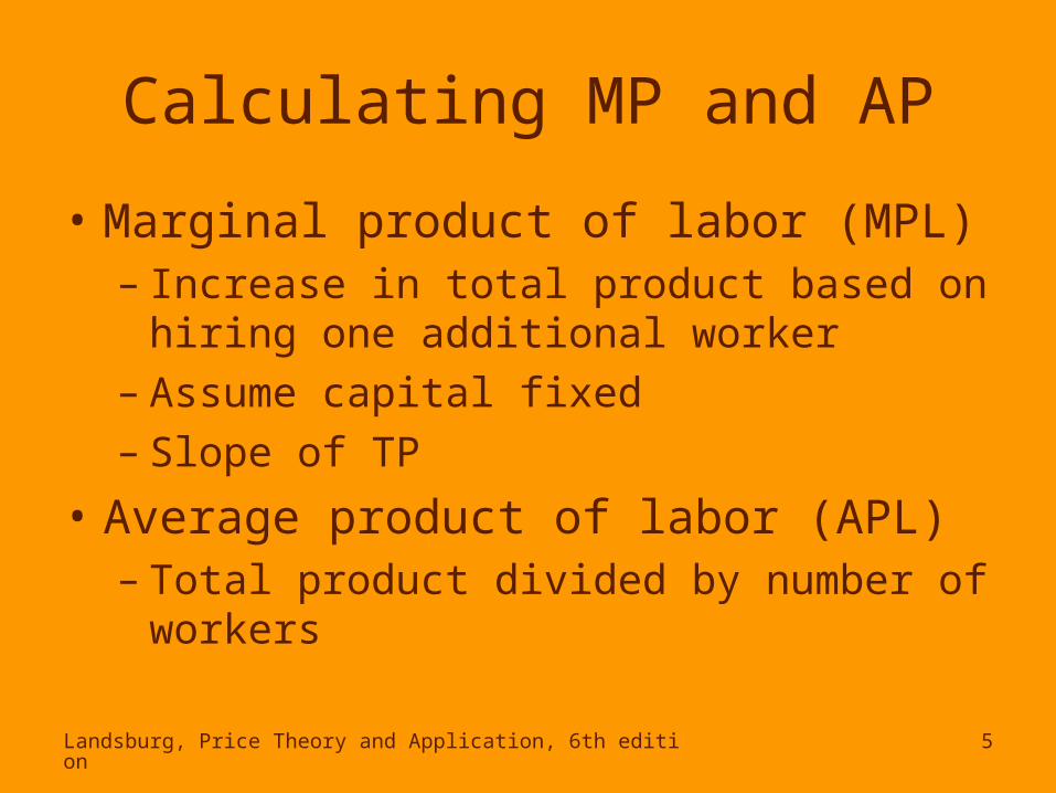
Calculating MP and AP
• Marginal product of labor (MPL) – Increase in total product based on hiring one
additional worker– Assume capital fixed– Slope of TP
• Average product of labor (APL) – Total product divided by number of workers
Landsburg, Price Theory and Application, 6th edition 6
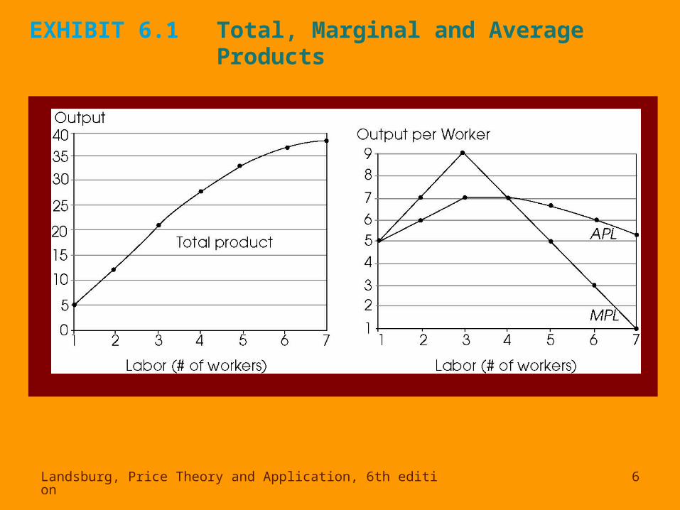
EXHIBIT 6.1 Total, Marginal and Average Products

Landsburg, Price Theory and Application, 6th edition 7
Shape of MP and AP Curves
• AP– If number of workers large, additional workers cause
average product of labor to decrease– Inverted U-shape
• MP– Inverted U-shape
• AP and MP relationship to one another– If MP > AP, MP lies above AP– If MP < AP, MP lies below AP– If MP = AP, AP at maximum or peak

Landsburg, Price Theory and Application, 6th edition 8
EXHIBIT 6.2 The Stages of Production
Landsburg, Price Theory and Application, 6th edition 9
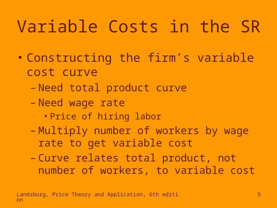
Variable Costs in the SR
• Constructing the firm’s variable cost curve– Need total product curve– Need wage rate
• Price of hiring labor
– Multiply number of workers by wage rate to get variable cost
– Curve relates total product, not number of workers, to variable cost
Landsburg, Price Theory and Application, 6th edition 10
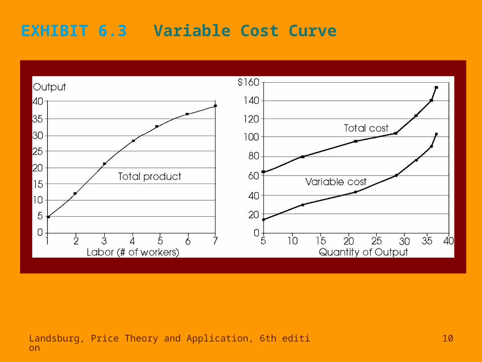
EXHIBIT 6.3 Variable Cost Curve
Landsburg, Price Theory and Application, 6th edition 11
Fixed Costs in the SR
• Costs of capital– Physical assets, such as machinery and
factories– Ex. handyman’s van
Landsburg, Price Theory and Application, 6th edition 12
Total Cost
• Total cost equal to sum of fixed and variable costs of production
• Additional cost considerations beside totals
Landsburg, Price Theory and Application, 6th edition 13
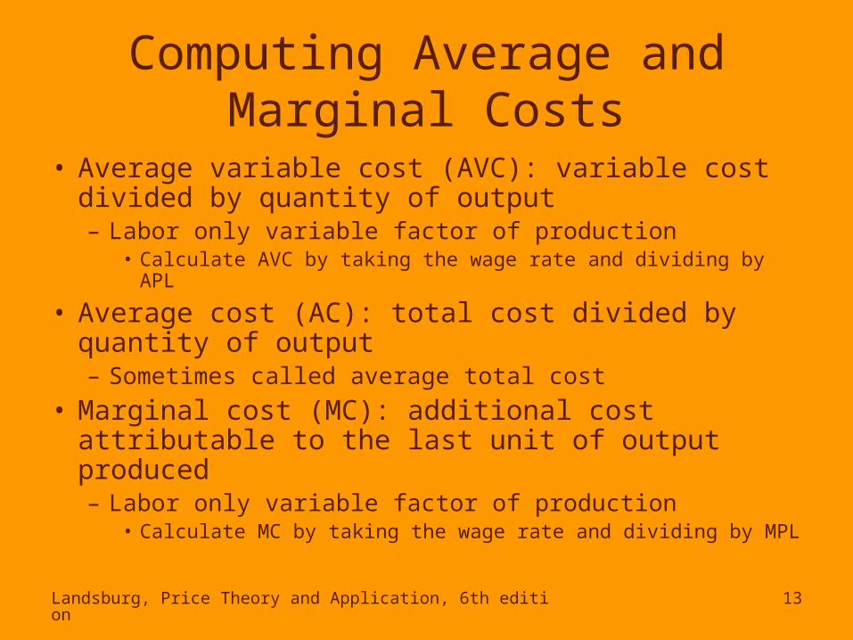
Computing Average and Marginal Costs
• Average variable cost (AVC): variable cost divided by quantity of output– Labor only variable factor of production
• Calculate AVC by taking the wage rate and dividing by APL
• Average cost (AC): total cost divided by quantity of output– Sometimes called average total cost
• Marginal cost (MC): additional cost attributable to the last unit of output produced– Labor only variable factor of production
• Calculate MC by taking the wage rate and dividing by MPL

Landsburg, Price Theory and Application, 6th edition 14
EXHIBIT 6.4 Deriving the Average and Marginal Cost Curves

Landsburg, Price Theory and Application, 6th edition 15
Shapes of Cost Curves
• VC curve always increasing– More output requires more labor– Higher costs
• TC curve determined by sum of FC and VC– FC constant– Has same shape as VC curve
• MC, AC, and AVC curves are U-shaped

Landsburg, Price Theory and Application, 6th edition 16
EXHIBIT 6.5The Geometry of Product Curves and Cost Curves
Landsburg, Price Theory and Application, 6th edition 17
Cost Curves Relations
• MC relationship to AVC and AC– MC below AVC, AVC falling– MC above AVC, AVC rising– MC equals AVC, AVC at minimum– Can replace AVC with AC, same holds true
• Shapes of cost curves related to shapes of product curves
Landsburg, Price Theory and Application, 6th edition 18
Production and Costs in the Long Run
• In long run (LR), firm can adjust employment of capital and labor
• Attempts to achieve the least cost method of producing a given quantity of output
Landsburg, Price Theory and Application, 6th edition 19
Isoquants
• Geometry of LR production– Label vertical axis with K, stands for capital– Label horizontal axis with L, which stands for labor– Fixed period of time
• Want to use least costly method– Avoid technologically inefficient points which are
outside the boundary• General observations
– Slope downward– Fill the plane– Never cross– Convex
Landsburg, Price Theory and Application, 6th edition 20
Marginal Rate of Technical Substitution
• Absolute value of slope of isoquant– MPL divided by MPK
• Amount of capital necessary to replace one unit of labor while maintaining a constant level of output
• If much labor and little capital employed to produce a unit of output, MRTSLK is small
• Geometrically isoquant is convex

Landsburg, Price Theory and Application, 6th edition 21
EXHIBIT 6.8 The Production Function
Landsburg, Price Theory and Application, 6th edition 22
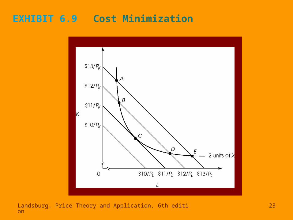
Choosing a Production Process
• Minimizing cost important part of maximizing profit
• Isocost allow to keep track of costs– Set of all baskets of inputs that can be employed at a
given cost– Slope: -PL/PK
• Minimizing cost and maximizing output requires firm choose tangency point between an isocost and an isoquant– Means that MRTS = PL/PK
– Tangencies lie along curve called the firm’s expansion path
Landsburg, Price Theory and Application, 6th edition 23
EXHIBIT 6.9 Cost Minimization
Landsburg, Price Theory and Application, 6th edition 24
Long-Run Cost Curves
• Information needed– Production function or isoquants– Input prices
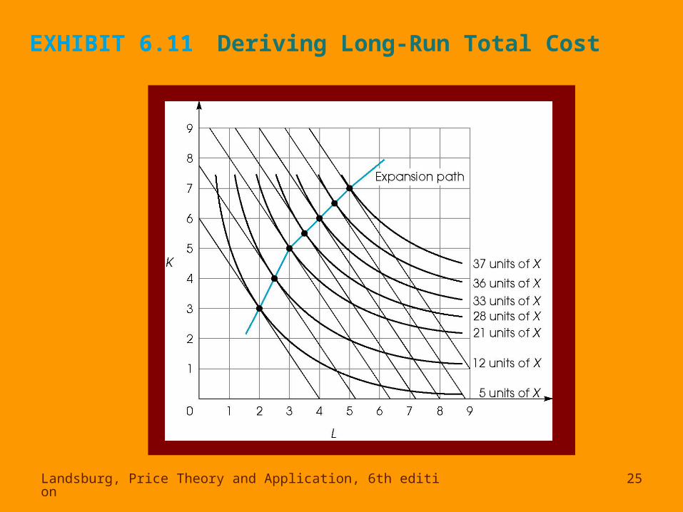
• Firm’s long-run total cost – Cost of producing a given amount of output when the
firm is able to operate on its expansion path• Long-run average cost
– Long-run total cost divided by quantity• Long-run marginal cost
– Part of long-run total cost attributable to the last unit produced
Landsburg, Price Theory and Application, 6th edition 25
EXHIBIT 6.11 Deriving Long-Run Total Cost

Landsburg, Price Theory and Application, 6th edition 26
EXHIBIT 6.12Long-Run Total, Marginal, and Average Costs

Landsburg, Price Theory and Application, 6th edition 27
Returns to Scale
• When all input quantities are increased by 1%, does output go up by– …more than 1%
• Increasing returns to scale• Occurs at low levels of output• Long-run average cost curve is decreasing
– …exactly 1%• Constant returns to scale• “What a firm can do one, it can do twice”• Long-run average cost curve is flat
– …less than 1%• Decreasing returns to scale• Occurs at sufficiently high levels of output• Long-run average cost curve is increasing

Landsburg, Price Theory and Application, 6th edition 28
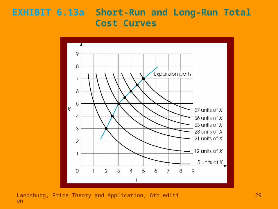
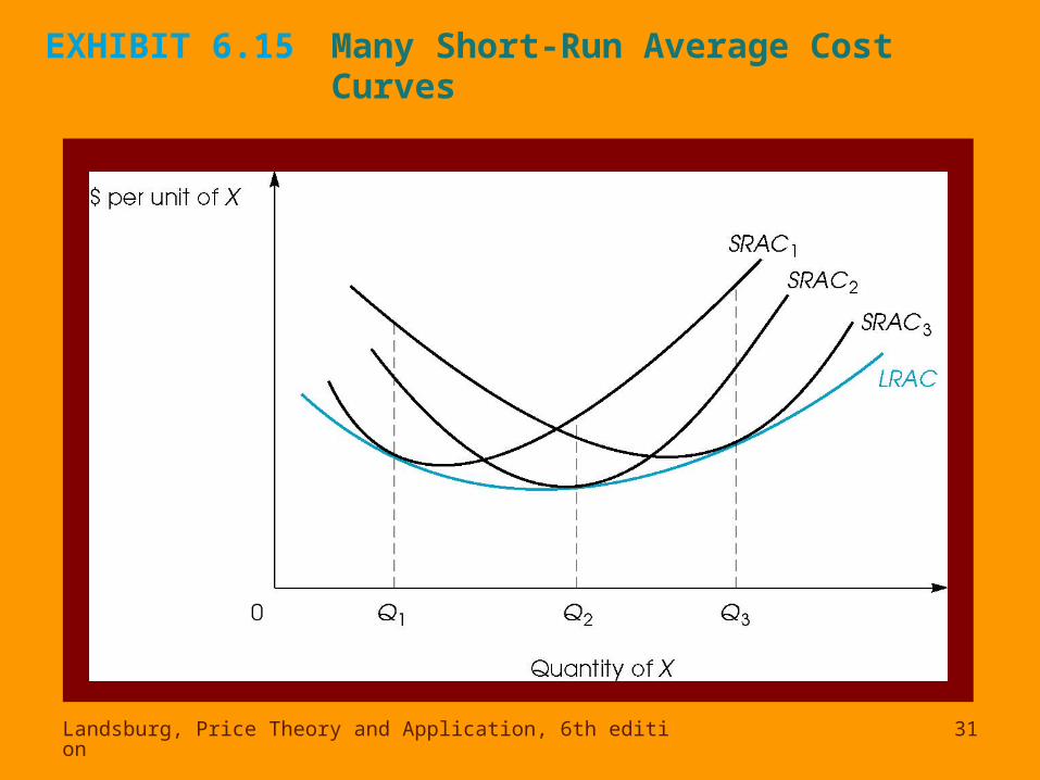
Relations between the SR and LR
• Derive SRTC from isoquants and factor prices• Derive LRTC from isoquants and factor prices• SRTC versus LRTC
– SRTC always at least as great as LRTC
• Multitude of short run situations– Each has different level of fixed capital– True for total cost and average cost– Each point on long-run curve is associated with a
tangency point from a short-run curve
Landsburg, Price Theory and Application, 6th edition 29
EXHIBIT 6.13a Short-Run and Long-Run Total Cost Curves

Landsburg, Price Theory and Application, 6th edition 30
EXHIBIT 6.13b Short-Run and Long-Run Total Cost Curves continued
Landsburg, Price Theory and Application, 6th edition 31
EXHIBIT 6.15 Many Short-Run Average Cost Curves


