Page 1
Stochastic Analysis of Life Insurance Surplus
by
Natalia Lysenko
B.Sc., Simon Fraser University, 2005.
a project submitted in partial fulfillment
of the requirements for the degree of
Master of Science
in the Department
of
Statistics and Actuarial Science
c© Natalia Lysenko 2006
SIMON FRASER UNIVERSITY
Summer 2006
All rights reserved. This work may not be
reproduced in whole or in part, by photocopy
or other means, without the permission of the author.
Page 2
APPROVAL
Name: Natalia Lysenko
Degree: Master of Science
Title of project: Stochastic Analysis of Life Insurance Surplus
Examining Committee: Dr. Carl J. Schwarz
Chair
Dr. Gary ParkerSenior SupervisorSimon Fraser University
Dr. Cary Chi-Liang TsaiSimon Fraser University
Dr. Richard LockhartExternal ExaminerSimon Fraser University
Date Approved:
ii
Page 3
Abstract
The behaviour of insurance surplus over time for a portfolio of homogeneous life
policies in an environment of stochastic mortality and rates of return is examined.
We distinguish between stochastic and accounting surpluses and derive their first two
moments. A recursive formula is proposed for calculating the distribution function of
the accounting surplus. We then examine the probability that the surplus becomes
negative in any given insurance year. Numerical examples illustrate the results for
portfolios of temporary and endowment life policies assuming an AR(1) process for
the rates of return.
Keywords: insurance surplus, stochastic rates of return, AR(1) process, stochas-
tic mortality, distribution function
iii
Page 4
Acknowledgements
I would like to thank the Department of Statistics and Actuarial Science
for providing a most encouraging and friendly environment for academic
growth, as well as for the consideration and flexibility that allowed me to
complete my degree in a very short period of time.
I am grateful to my examining committee, Dr. Cary Tsai and Dr. Richard
Lockhart, for their very careful reading of the report and valuable com-
ments that helped to perfect its final version.
I am deeply indebted to my supervisor Dr. Gary Parker for his excellent
guidance throughout my graduate studies, for his expertise and enthusi-
asm about the field of actuarial science, for all the time devoted to helpful
discussions and reviewing the drafts of this project, for giving me an op-
portunity and freedom to discover my own research interests and follow
them, for expecting independence, for his constant encouragement and
positive attitude. I am thankful to him for setting a great example of
dedication to the academia that I am sure will stay with me in the years
to come and become a source of inspiration in my future pursuits.
This journey would have been much rougher and less enjoyable without
continuous support from my close friends. Many thanks to Monica Lu for
cheering me up and sharing so many happy and sad moments with me. I
am especially grateful to Matt Pratola for his generous help in so many
difficult situations, for his willingness to listen and understand, for being
an example of extreme patience and perfectionism.
Last but not least, I owe a great debt of gratitude to my parents for their
iv
Page 5
love, support, understanding and patience; for bringing me to Canada
and giving me an opportunity to do what I like doing the most - studying.
Without my mother’s care and my father’s strong belief in me, I do not
think that I would be able to go this far.
v
Page 6
Contents
Approval . . . . . . . . . . . . . . . . . . . . . . . . . . . . . . . . . . . . . ii
Abstract . . . . . . . . . . . . . . . . . . . . . . . . . . . . . . . . . . . . . iii
Acknowledgements . . . . . . . . . . . . . . . . . . . . . . . . . . . . . . . iv
Contents . . . . . . . . . . . . . . . . . . . . . . . . . . . . . . . . . . . . . vi
List of Tables . . . . . . . . . . . . . . . . . . . . . . . . . . . . . . . . . . viii
List of Figures . . . . . . . . . . . . . . . . . . . . . . . . . . . . . . . . . . x
1 Introduction . . . . . . . . . . . . . . . . . . . . . . . . . . . . . . . . 1
2 Model Assumptions . . . . . . . . . . . . . . . . . . . . . . . . . . . . 9
2.1 Stochastic Rates of Return . . . . . . . . . . . . . . . . . . . . 9
2.2 Decrements . . . . . . . . . . . . . . . . . . . . . . . . . . . . 15
2.3 Summary of Assumptions . . . . . . . . . . . . . . . . . . . . 16
3 Single Policy . . . . . . . . . . . . . . . . . . . . . . . . . . . . . . . . 17
3.1 Methodology . . . . . . . . . . . . . . . . . . . . . . . . . . . 17
3.2 Numerical Illustrations . . . . . . . . . . . . . . . . . . . . . . 23
4 Homogeneous Portfolio . . . . . . . . . . . . . . . . . . . . . . . . . . 29
4.1 Retrospective Gain . . . . . . . . . . . . . . . . . . . . . . . . 30
4.2 Prospective Loss . . . . . . . . . . . . . . . . . . . . . . . . . 32
4.3 Insurance Surplus . . . . . . . . . . . . . . . . . . . . . . . . . 35
4.3.1 Introduction . . . . . . . . . . . . . . . . . . . . . . 35
4.3.2 Methodology . . . . . . . . . . . . . . . . . . . . . . 36
vi
Page 7
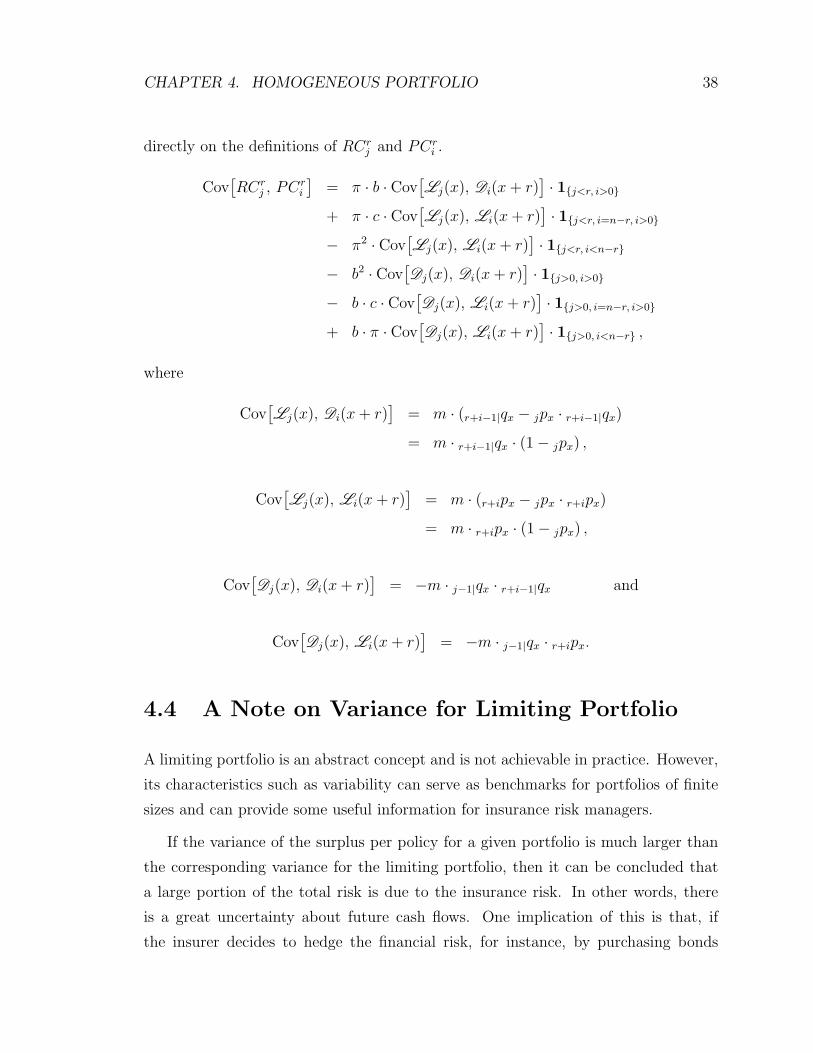
4.4 A Note on Variance for Limiting Portfolio . . . . . . . . . . . 38
4.5 Numerical Illustrations . . . . . . . . . . . . . . . . . . . . . . 39
5 Distribution Function of Accounting Surplus . . . . . . . . . . . . . . 55
5.1 Distribution Function of Accounting Surplus . . . . . . . . . . 56
5.2 Distribution Function of Accounting Surplus for Limiting Port-
folio . . . . . . . . . . . . . . . . . . . . . . . . . . . . . . . . 59
5.3 Numerical Illustrations of Results . . . . . . . . . . . . . . . . 60
5.3.1 Example 1: Portfolio of Endowment Life Insurance
Policies . . . . . . . . . . . . . . . . . . . . . . . . . 60
5.3.2 Example 2: Portfolio of Temporary Life Insurance
Policies . . . . . . . . . . . . . . . . . . . . . . . . . 66
6 Conclusions . . . . . . . . . . . . . . . . . . . . . . . . . . . . . . . . 72
Appendices . . . . . . . . . . . . . . . . . . . . . . . . . . . . . . . . . . . 75
A Additional Material . . . . . . . . . . . . . . . . . . . . . . . . . . . . 75
A.1 Interest Rate Model . . . . . . . . . . . . . . . . . . . . . . . 75
A.2 Theorem 1 . . . . . . . . . . . . . . . . . . . . . . . . . . . . . 76
A.3 Retrospective Cash Flows Conditional on
Number of Policies In Force . . . . . . . . . . . . . . . . . . . 76
A.4 On Benefit Premium Determination . . . . . . . . . . . . . . . 78
A.5 Proof of Result 4.3.1 . . . . . . . . . . . . . . . . . . . . . . . 79
B On Numerical Computations . . . . . . . . . . . . . . . . . . . . . . . 83
C Mortality Table . . . . . . . . . . . . . . . . . . . . . . . . . . . . . . 91
D Distribution Function of Accounting Surplus . . . . . . . . . . . . . . 92
Bibliography . . . . . . . . . . . . . . . . . . . . . . . . . . . . . . . . . . 96
vii
Page 8
List of Tables
3.1 Expected values and standard deviations of retrospective gain, prospec-
tive loss and surplus for 5-year temporary insurance contract. . . . . 25
3.2 Expected values and standard deviations of retrospective gain, prospec-
tive loss and surplus for 5-year endowment insurance contract. . . . . 26
4.1 Standard deviations of retrospective gain per policy for portfolios of
5-year temporary insurance contracts. . . . . . . . . . . . . . . . . . . 43
4.2 Standard deviations of retrospective gain per policy for portfolios of
5-year endowment insurance contracts. . . . . . . . . . . . . . . . . . 44
4.3 Standard deviations of prospective loss per policy for portfolios of 5-
year temporary insurance contracts. . . . . . . . . . . . . . . . . . . 45
4.4 Standard deviations of prospective loss per policy for portfolios of 5-
year endowment insurance contracts. . . . . . . . . . . . . . . . . . . 46
4.5 Standard deviations of accounting surplus per policy for portfolios of
5-year temporary insurance contracts. . . . . . . . . . . . . . . . . . 47
4.6 Standard deviations of accounting surplus per policy for portfolios of
5-year endowment insurance contracts. . . . . . . . . . . . . . . . . . 48
4.7 Standard deviations of stochastic surplus per policy for portfolios of
5-year temporary insurance contracts. . . . . . . . . . . . . . . . . . 49
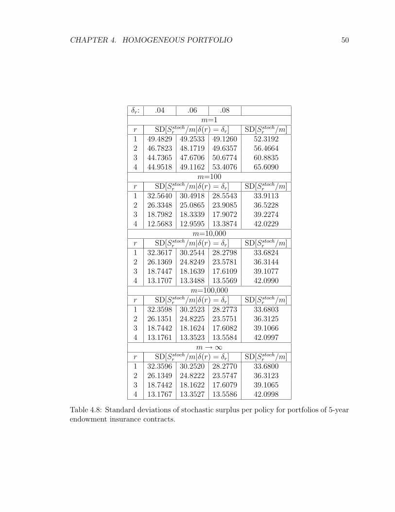
4.8 Standard deviations of stochastic surplus per policy for portfolios of
5-year endowment insurance contracts. . . . . . . . . . . . . . . . . . 50
viii
Page 9
4.9 Correlation coefficients between retrospective gain and prospective loss
per policy for portfolios of 5-year endowment insurance contracts. . . 51
5.1 Estimates of probabilities that accounting surplus falls below zero for
a portfolio of 100 10-year endowment policies. . . . . . . . . . . . . . 62
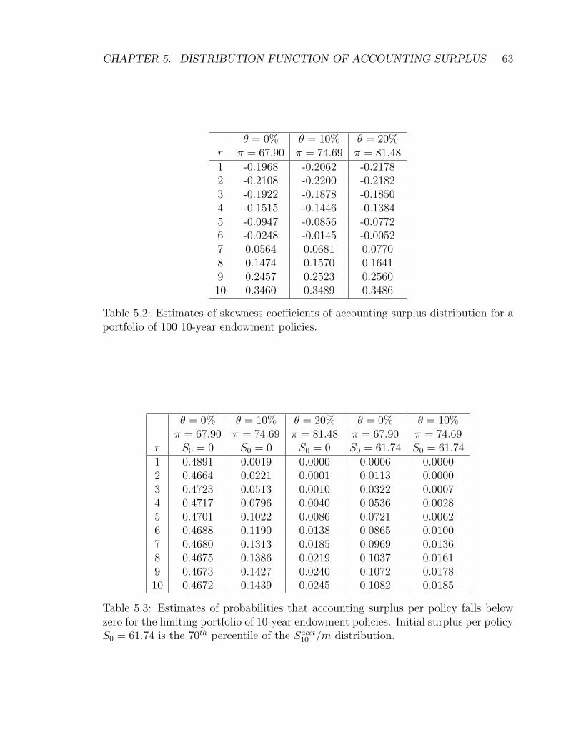
5.2 Estimates of skewness coefficients of accounting surplus distribution
for a portfolio of 100 10-year endowment policies. . . . . . . . . . . . 63
5.3 Estimates of probabilities that accounting surplus falls below zero for
the limiting portfolio of 10-year endowment policies. . . . . . . . . . . 63
5.4 Estimates of skewness coefficients of accounting surplus distribution
for the limiting portfolio of 10-year endowment policies. . . . . . . . . 66
5.5 Estimates of probabilities that accounting surplus falls below zero for
a portfolio of 1000 5-year temporary policies. . . . . . . . . . . . . . . 67
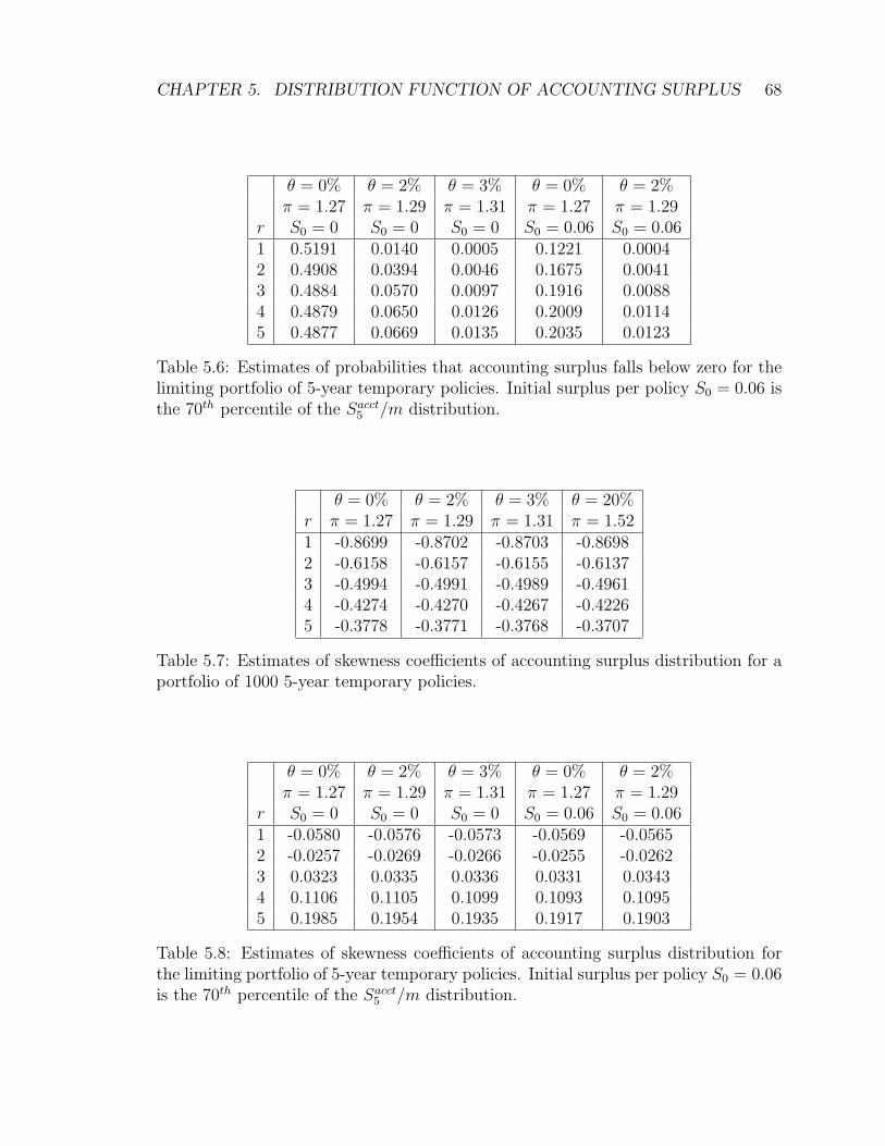
5.6 Estimates of probabilities that accounting surplus falls below zero for
the limiting portfolio of 5-year temporary policies. . . . . . . . . . . . 68
5.7 Estimates of skewness coefficients of accounting surplus distribution
for a portfolio of 1000 5-year temporary policies. . . . . . . . . . . . . 68
5.8 Estimates of skewness coefficients of accounting surplus distribution
for the limiting portfolio of 5-year temporary policies. . . . . . . . . . 68
B.1 Estimates of expected values and standard deviations of accounting
surplus per policy for a portfolio of 100 10-year endowment policies. . 87
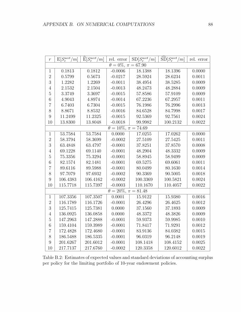
B.2 Estimates of expected values and standard deviations of accounting
surplus per policy for the limiting portfolio of 10-year endowment policies. 88
B.3 Estimates of expected values and standard deviations of accounting
surplus per policy for a portfolio of 1000 5-year temporary policies. . 89
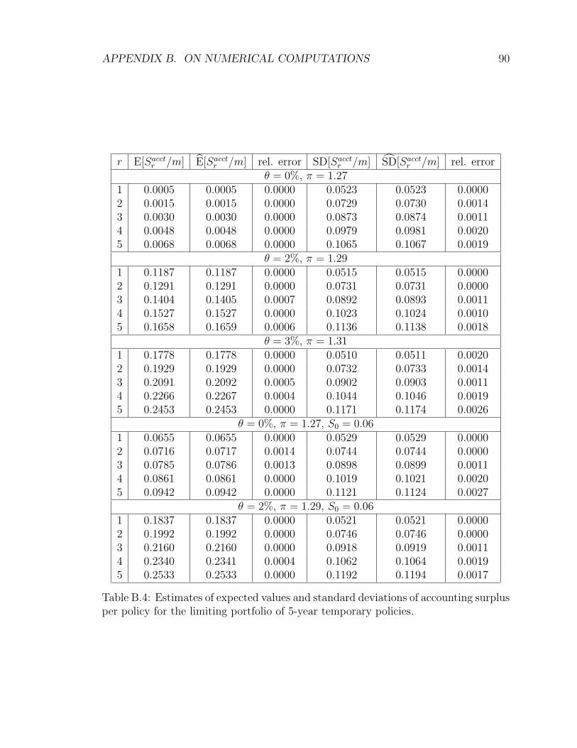
B.4 Estimates of expected values and standard deviations of accounting
surplus per policy for the limiting portfolio of 5-year temporary policies. 90
ix
Page 10
List of Figures
3.1 Expected values and standard deviations of retrospective gain, prospec-
tive loss and surplus for 10-year temporary and endowment contracts. 27
3.2 Expected values and standard deviations of retrospective gain, prospec-
tive loss and surplus for 25-year temporary and endowment contracts. 28
4.1 Expected value and standard deviations of accounting and stochastic
surpluses. . . . . . . . . . . . . . . . . . . . . . . . . . . . . . . . . . 52
4.2 Conditional standard deviation of surplus per policy for a portfolio of
100 10-year temporary contracts. . . . . . . . . . . . . . . . . . . . . 53
4.3 Conditional standard deviation of surplus per policy for a portfolio of
100 10-year endowment contracts. . . . . . . . . . . . . . . . . . . . . 54
5.1 Distribution functions of accounting surplus per policy for a portfolio
of 100 10-year endowment policies. . . . . . . . . . . . . . . . . . . . 64
5.2 Distribution functions of accounting surplus per policy for the limiting
portfolio of 10-year endowment contracts. . . . . . . . . . . . . . . . . 65
5.3 Distribution functions of accounting surplus per policy for a portfolio
of 1000 5-year temporary policies. . . . . . . . . . . . . . . . . . . . . 69
5.4 Distribution functions of accounting surplus per policy for the limiting
portfolio of 5-year temporary policies. . . . . . . . . . . . . . . . . . . 70
5.5 Density functions of accounting surplus per policy for the limiting port-
folio of 5-year temporary policies. . . . . . . . . . . . . . . . . . . . . 71
x
Page 11
Chapter 1
Introduction
Understanding stochastic properties of life insurance surplus is essential for insur-
ance companies to make business decisions that will guarantee a high probability of
solvency. Life insurers face a variety of risks. How many death benefits have to be
paid out in any given year? Uncertain timing of contingent cash flows gives rise to
mortality or insurance risk. A life insurance policy is typically purchased by a series
of periodic payments called (contract) premiums. This series of payments contingent
on policyholders survival to the time when each payment comes due constitutes a life
annuity of premiums. The premiums are invested in the market to earn interest. But
what interest rates will prevail in the market in the future? Many insurance con-
tracts have a fairly long term (think, for example, of a whole life insurance issued to
someone aged 30), in which case ignoring the stochastic nature of rates of return will
lead to a significant understatement of the true riskiness of these contracts. There
are other sources of uncertainty arising in the life insurance context (future expenses,
lapses, etc.), but the environment of stochastic mortality and rates of return already
presents many challenges for analyzing life insurance contracts.
The theory of life contingencies evolved from a deterministic treatment of various
risks to the introduction of a methodology for the stochastic treatment of decrements
at first and later of rates of return. Traditionally, in order to take into account differ-
ent sources of risk, including decrements due to mortality, disability, etc. as well as
interest rates, deterministic discounting for each source of risk was used (see Jordan
1
Page 12
CHAPTER 1. INTRODUCTION 2
(1967)). However, under this approach it was impossible to obtain information about
the likelihood and magnitude of random deviations from the mean discounted values.
In the text by Bowers et al. (1986), the theory of life contingencies was extended to
incorporate the random nature of decrements. The concept of a random survivor-
ship group was introduced by relating the survival function and the life table, which
allowed for the full use of probability theory; whereas, the so-called deterministic sur-
vivorship group approach, previously used in actuarial science and based on the rates
(as opposed to probabilities) of decrement summarized in the life table, did not have
this flexibility and thus ignored the stochastic nature of mortality. Under this frame-
work the mortality risk can be quantified by considering such summary measures as
standard deviation, median and percentiles of actuarial functions’ distributions.
Although mortality risk is definitely an important risk component of the life in-
surance business, in many circumstances it can be at least partially diversified by
increasing the size of the business. On the other hand, investment risk cannot be
diversified and in some cases its relative size can be quite large. Thus, models for
stochastic rates of return must be incorporated in the theory of life contingencies.
Search for a useful model for rates of return that can be employed in actuarial
applications can be traced back to the 1970’s. Since by now there is a very extensive
literature on this topic, no attempt is made here to provide a complete list of related
papers. Instead, some of the key papers are mentioned to demonstrate what kind of
models have been considered and in what applications they were used.
Before choosing a model for stochastic rates of return, one needs to decide, first
of all, what exactly has to be modeled since there are several possibilities including
an effective interest rate, force of interest and force of interest accumulation function.
Other questions that have to be addressed are related to the dependence structure
of rates of return in successive time intervals (i.e., should the rates be assumed to
be independent or correlated?) and the type of model (i.e., should a continuous or
discrete time framework be used?). This fairly wide range of possibilities for modeling
interest rate randomness led researchers to consider a variety of models.
In a number of early papers on the subject it was assumed that the forces of
interest in successive years were uncorrelated and identically distributed (i.e., the force
Page 13
CHAPTER 1. INTRODUCTION 3
of interest is generated by a white noise process). Waters (1978) used this assumption
to calculate the first four moments of the compound interest and actuarial functions
and to obtain the limiting distribution of the average sums of actuarial functions
by fitting Pearson curves. This assumption about rates of return was also made by
Boyle(1976) and Dufresne (1990) among others.
A more realistic assumption is to assume that the forces of interest in successive
years are correlated. Various time series models have been employed for this purpose.
For example, Pollard (1971) used an autoregressive process of order two.
Panjer and Bellhouse (1980) developed a general theory for both discrete and con-
tinuous stochastic interest models for determining the moments of the present value
of deterministic and contingent cash flows. Then the authors specifically considered
discrete time autoregressive models of order one and two (with real roots of charac-
teristic polynomial only) as well as their continuous time analogue and applied their
results to a whole life insurance policy and a life annuity. A shortcoming of this paper
is that by considering stationary autoregressive models, future rates of return are as-
sumed to be independent of past and current rates. In Bellhouse and Panjer (1981),
the results were extended to models in which forces of interest depend on a number
of past and current rates. This was achieved by using discrete time conditional au-
toregressive processes. Numerical illustrations for the price of a pure discount bond,
an annuity certain, a whole life insurance and a life annuity were provided assuming
a conditional autoregressive process of order one.
Dhaene (1989) further extended the work done by Panjer and Bellhouse as well as
by Giaccotto (1986) to the case when the force of interest follows an autoregressive
integrated moving average process of order (p, d, q), ARIMA (p, d, q). The paper
presented a methodology for efficient computation of the moments of present value
functions.
Stochastic differential equations (SDE) also found their use in the actuarial lit-
erature. For example, Beekman and Fuelling (1990) used the Ornstein-Uhlenbeck
process (a first order linear SDE, also known as the Vasicek model in the finance
literature) to model the force of interest accumulation function. As an application,
they derived formulas for the mean values and standard deviations of future payment
Page 14
CHAPTER 1. INTRODUCTION 4
streams, both deterministic (an annuity certain) and contingent (a life annuity). Nu-
merical examples illustrated the results for different values of parameters. In a series
of publications by Parker (e.g., Parker (1993), Parker (1994a), Parker (1996) and
Parker (1997)), the author also used the Ornstein-Uhlenbeck process but for the
force of interest rather than for the force of interest accumulation function. In addi-
tion, Parker (1995) studied a second order linear stochastic differential equation for
the force of interest process. Three cases for the roots of the characteristic equation
were considered (real and distinct roots, real and equal roots, and complex roots).
It was demonstrated in the paper that this model is able to combine the effects of a
tendency to continue a recent trend and of a mean reverting property. This indicates
that a second order process is more flexible compared to a first order process, which
could only have one of those properties, usually the mean reversion. Numerical ex-
amples were given for the expected value and variance of a discounting function and
an annuity certain.
A couple of remarks can be made at this point. In some cases, whether a discrete
model or a continuous one is used does not alter the dynamic of the process. For ex-
ample, a conditional AR(1) process is the discrete analogue of the Ornstein-Uhlenbeck
process; also a discrete representation of a second order SDE is the ARMA(2,1) pro-
cess. So, a choice of a discrete or a continuous model can be a personal preference.
Refer to the text by Pandit and Wu (1983) for a discussion of the principle of covari-
ance equivalence that can be used to establish parametric relations between discrete
and continuous representations of a process.
It can be noted that some of the researcher chose to model the force of interest and
others the force of interest accumulation function. In the paper by Parker (1994b)
the difference between these two modeling approaches was discussed. Numerical
illustrations of the expected value, standard deviation and skewness of an annuity
immediate for a number of processes under each of the two approaches were presented,
which demonstrated a different stochastic behavior of present value functions under
the two modeling methods. Further, to provide more insight into the implicit behavior
of the force of interest process under the two approaches, the conditional expected
value of the force of interest accumulation function up to time t given its value up to
time s (s < t) and the force of interest at time s was examined. It was revealed that
Page 15
CHAPTER 1. INTRODUCTION 5
this conditional expectation does not depend on the value of the force of interest at
time s when modeling the force of interest accumulation function. It is more realistic
to assume that this conditional expectation depends on the force of interest at time s,
which is the case when modeling the force of interest. A numerical example indicated
that one possible implication of modeling the force of interest accumulation function
is that the expected value of the force of interest in the immediate future can be
significantly away from its current value. This illustration shows that modeling the
force of interest accumulation function has limited practical value.
Most of the papers mentioned above gave the first two or three moments of present
value and actuarial functions when only one stream of payments or only one policy
was considered. Some generalizations to these applications include studying the whole
distribution (either using the density function or the cumulative distribution function)
for a portfolio of identical contracts or a general portfolio.
Frees (1990) presented the first two moments of the net single premium of a single
insurance contract and an annuity. Premium determination under the equivalence
principle and explicit extension to reserves including the second moment of the loss
function were presented. The results were derived at first assuming that the forces of
interest in each time interval are independent and identically distributed (i.i.d.) each
following the same normal distribution and then using a moving average process of
order one, MA(1). In the second part of the paper, the author considered a block of
business. He proposed to approximate the distribution of the average loss random
variable for a block of identical policies by another random variable, which is equal
to the expected value of the loss random variable for one policy where expectation is
taken over time-of-death random variable and follows the limiting distribution of the
average loss when the number of policies in the block approaches infinity. A suggestion
for a recursive calculation of the distribution function of the average loss under the
i.i.d. assumption for interest rates was given. Finally, the limiting distribution of
surplus, defined as the excess of assets over liabilities, for the case of full matching of
assets and projected liabilities was presented.
Norberg (1993) derived the expected value and variance of the liability associated
with one contract and then of the total liability for a portfolio of policies assuming the
Ornstein-Uhlenbeck process for the force of interest. He proposed a simple solvency
Page 16
CHAPTER 1. INTRODUCTION 6
criterion, which requires an insurer to maintain a reserve equal to the expected value
plus a multiple of the standard deviation of the loss random variable. Numerical
results for an authentic portfolio were provided.
The expected value, standard deviation and coefficient of skewness as well as an
approximate distribution of the present value of future deterministic cash flows when
the force of interest is modeled by the white noise process, the Wiener process and
the Ornstein-Uhlenbeck process were presented in Parker (1993). The approximation
of the cumulative distribution function was based on a recursive integral equation.
An n-year certain annuity-immediate was used for numerical illustrations. The same
approximation technique for the distribution function was then applied to the lim-
iting portfolios of identical temporary and endowment insurance contracts in Parker
(1994a) and Parker (1996) with the Ornstein-Uhlenbeck process for the force of in-
terest used for illustrative purposes (see Coppola et al. (2003) for an application of
the method to large annuity portfolios). In Parker (1997), these results were further
generalized to a general limiting portfolio of different life insurance policies such as
temporary, endowment and whole life. In addition, this paper discussed a way of
splitting the riskiness of the portfolio into an insurance risk and an investment risk
(see also Bruno et al. (2000)). Although high accuracy of the approximation used
by the author in the above-mentioned papers was justified, Parker (1998) presented a
method for obtaining the exact distribution of the discounted and accumulated val-
ues of deterministic cash flows based on recursive double integral equations. The two
results that will be derived in Chapter 5 use a variation of this method.
Marceau et al.(1999) studied the prospective loss random variable for general
portfolios of life insurance contacts and compared its first two moments as well as the
distribution functions obtained via Monte Carlo simulation method for portfolios of
different sizes (including a limiting portfolio) and different composition. Numerical
examples for portfolios of temporary, endowment and a combination of temporary and
endowment life policies, in which the force of interest assumed to follow a conditional
AR(1) process, were presented. It was observed that the convergence rate of the
variance of the loss random variable for a portfolio of temporary contracts is much
slower compared to the other two portfolios. This indicates that the mortality risk
component is large compared to the non-diversifiable investment risk in any portfolio
Page 17
CHAPTER 1. INTRODUCTION 7
of a realistic size, and as a result of this a use of the distribution of the limiting
portfolio to approximate the distribution of a finite portfolio is questionable in a
context of temporary life insurances.
Another approximation for the distribution of the loss random variable for a single
life annuity and for a homogeneous portfolio is given in Hoedemakers (2005). This
approximation is based on the concept of comonotonicity. Upper and lower bounds on
quantiles of a distribution were obtained and their convex combination was demon-
strated to be a very accurate approximation of the true distribution. The authors
chose to model the force of interest accumulation function by a Brownian motion with
a drift and an Ornstein-Uhlenbeck process.
The focus of the papers mentioned above is on the stochastically discounted value
of future deterministic or contingent cash flows with the cash flows being viewed
and valued at the same point in time. For example, the net single premium of a
life insurance policy or a life annuity is viewed and valued at the issue date. In the
reserve calculation only cash flows that will be incurred by the inforce policies at a
given valuation date are taken into account and the experience of the portfolio prior
to that valuation date is ignored. In the case of a single policy, if the policyholder
does not survive to a given valuation date, no reserve is allocated for that policy.
We will develop a model and perform our analysis in a different framework. To
illustrate our approach consider a closed block of life insurance business at its initia-
tion. All the quantities of interest that we study are measured at some given dates
in the future but are viewed at the initiation date. This framework allows assessing
adequacy of, for example, initial surplus level, pricing and future reserving method
before the block of business is launched.
Let us follow this block of business in time. Fix one of the valuation dates and
refer to it as time r. Prior to time r, the insurer collects premiums and pays death
benefits according to the terms of the contract. So, by time r, the insurer’s assets
from this block of business are equal to the accumulated value of past premiums net
of death benefits paid. After time r, the insurer will continue paying benefits as they
come due and receive periodic premiums. The discounted value at time r of all future
benefits net of all future premiums to be collected constitutes the insurer’s liabilities.
Page 18
CHAPTER 1. INTRODUCTION 8
The value of assets in excess of the value of liabilities represents the surplus. It is this
quantity that we attempt to study. It is worth mentioning at this point that in the
context of a portfolio of life insurance policies we will distinguish between two types
of surplus. One of them we call a stochastic surplus, which was briefly described in
general terms above. The other type of surplus we refer to as an accounting surplus.
Although the name may suggest a deterministic nature of the accounting surplus, in
fact it is a stochastic quantity. The difference between the two types of surplus lies
in how liabilities are defined. In the case of accounting surplus the liability is the
actuarial reserve, which is typically some summary measure (e.g., expected value) or
a statistic of the prospective loss random variable, whereas in the case of stochastic
surplus it is the prospective loss random variable itself.
For insurance regulators it is important that insurance companies maintain an
adequate surplus level. To represent actuarial liabilities, the insurers are required to
report their actuarial reserves calculated in accordance with regulations. So, when
monitoring insurance companies, the regulators actually look at what we call the
accounting surplus. We propose a formula for obtaining the distribution function
of accounting surplus at any given valuation date. One piece of information that is
readily available from this distribution function is the probability that the surplus
falls below zero at any given time r. If this probability is too high, say above 5%,
then perhaps the insurer should make some adjustments to the terms of the contract
such as, for example, increasing the premium rate or raising additional initial surplus.
Assumptions regarding the model for rates of return and decrements due to mor-
tality are presented in Chapter 2. In Chapter 3 we develop a methodology for studying
a single life insurance policy. The ideas for one policy are further extended to study
a portfolio of homogeneous policies in Chapters 4 and 5. In Chapter 4 we define two
types of insurance surpluses and derive their first two moments. A method for com-
puting the distribution function of the accounting surplus is discussed in Chapter 5.
Concluding remarks and areas for future research are provided in Chapter 6.
Page 19
Chapter 2
Model Assumptions
2.1 Stochastic Rates of Return
For illustrative purposes, we choose to model the force of interest by a conditional
autoregressive process of order one, AR(1). A similar model was used, for example,
by Bellhouse and Panjer (1981) and Marceau et al. (1999). However, the results that
will be presented in the later chapters may also allow the use of other more general
Gaussian models.
Let δ(k) be the force of interest in period (k−1, k], k = 1, 2, . . . , n, with a possible
realization denoted by δk. The forces of interest {δ(k); k = 1, 2, . . . , n} satisfy the
following autoregressive model:
δ(k)− δ = φ [δ(k − 1)− δ] + εk, (2.1)
where εk ∼N(0, σ2) and δ is the long-term mean of the process. We assume that
|φ| < 1 to ensure stationarity of the process.
For our further discussion, it is convenient to introduce a notation for the force
of interest accumulation function, which is then used to study both discounting and
accumulation processes.
Let I(s, r) denote the force of interest accumulation function between times s and
9
Page 20
CHAPTER 2. MODEL ASSUMPTIONS 10
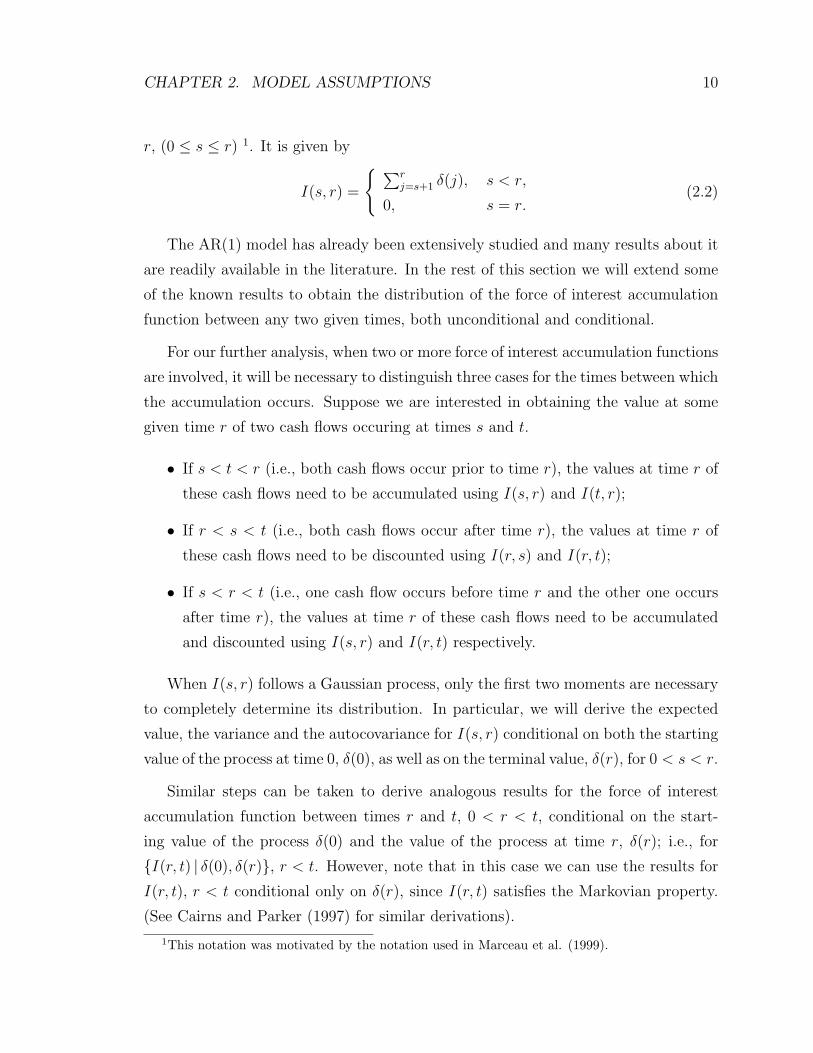
r, (0 ≤ s ≤ r) 1. It is given by
I(s, r) =
{ ∑rj=s+1 δ(j), s < r,
0, s = r.(2.2)
The AR(1) model has already been extensively studied and many results about it
are readily available in the literature. In the rest of this section we will extend some
of the known results to obtain the distribution of the force of interest accumulation
function between any two given times, both unconditional and conditional.
For our further analysis, when two or more force of interest accumulation functions
are involved, it will be necessary to distinguish three cases for the times between which
the accumulation occurs. Suppose we are interested in obtaining the value at some
given time r of two cash flows occuring at times s and t.
• If s < t < r (i.e., both cash flows occur prior to time r), the values at time r of
these cash flows need to be accumulated using I(s, r) and I(t, r);
• If r < s < t (i.e., both cash flows occur after time r), the values at time r of
these cash flows need to be discounted using I(r, s) and I(r, t);
• If s < r < t (i.e., one cash flow occurs before time r and the other one occurs
after time r), the values at time r of these cash flows need to be accumulated
and discounted using I(s, r) and I(r, t) respectively.
When I(s, r) follows a Gaussian process, only the first two moments are necessary
to completely determine its distribution. In particular, we will derive the expected
value, the variance and the autocovariance for I(s, r) conditional on both the starting
value of the process at time 0, δ(0), as well as on the terminal value, δ(r), for 0 < s < r.
Similar steps can be taken to derive analogous results for the force of interest
accumulation function between times r and t, 0 < r < t, conditional on the start-
ing value of the process δ(0) and the value of the process at time r, δ(r); i.e., for
{I(r, t) | δ(0), δ(r)}, r < t. However, note that in this case we can use the results for
I(r, t), r < t conditional only on δ(r), since I(r, t) satisfies the Markovian property.
(See Cairns and Parker (1997) for similar derivations).
1This notation was motivated by the notation used in Marceau et al. (1999).
Page 21
CHAPTER 2. MODEL ASSUMPTIONS 11
To calculate the moments of I(s, r), 0 < s < r, conditional on δ(0) and δ(r), it
is convenient first to derive the unconditional moments of I(s, r), 0 < s < r (i.e.,
moments for the stationary distribution of I(s, r), 0 < s < r), which are then used
to obtain the moments of I(s, r), 0 < s < r, conditional only on the starting value,
δ(0), and consequently on both the starting and the terminal values of the process.
It is well known that for the stationary AR(1) process defined in (2.1)
E[δ(j)] = δ,
Cov[δ(i), δ(j)] =σ2
1− φ2φ|i−j|.
Then, for s < r,
E[I(s, r)] = E[ r∑
j=s+1
δ(j)]
=r∑
j=s+1
E[δ(j)] = (r − s)δ (2.3)
and
Var[I(s, r)] = Var[r∑
j=s+1
δ(j)]
=r∑
j=s+1
r∑i=s+1
Cov[δ(j), δ(i)]
= (r − s) Var[δ(j)] + 2r−1∑
j=s+1
r∑i=j+1
Cov[δ(j), δ(i)]
= (r − s)σ2
1− φ2 + 2r−1∑
j=s+1
r∑i=j+1
σ2
1− φ2φi−j
=σ2
1− φ2 [r − s+ 2φ
1− φ(r − s− 1− φ
1− φ(1− φr−s−1))]. (2.4)
The covariance terms, corresponding to the three cases for the force of interest
accumulation functions mentioned earlier, are given by the following formulas:
Page 22
CHAPTER 2. MODEL ASSUMPTIONS 12
Case 1: s < t < r
Cov[I(s, r), I(t, r)] =r∑
i=s+1
r∑j=t+1
Cov[δ(i), δ(j)]
=r∑
i=t+1
r∑j=t+1
Cov[δ(i), δ(j)] +t∑
i=s+1
r∑j=t+1
Cov[δ(i), δ(j)]
= Var[I(t, r)] +t∑
i=s+1
r∑j=t+1
σ2
1− φ2φj−i
= Var[I(t, r)] +σ2
1− φ2
φ
(1− φ)2 (φt − φr)(φ−t − φ−s).
Case 2: r < s < t
Cov[I(r, s), I(r, t)] =s∑
i=r+1
t∑j=r+1
Cov[δ(i), δ(j)]
=s∑
i=r+1
s∑j=r+1
Cov[δ(i), δ(j)] +s∑
i=r+1
t∑j=s+1
Cov[δ(i), δ(j)]
= Var[I(r, s)] +s∑
i=r+1
t∑j=s+1
σ2
1− φ2φj−i
= Var[I(r, s)] +σ2
1− φ2
φ
(1− φ)2 (φs − φt)(φ−s − φ−r).
Case 3: s < r < t
Cov[I(s, r), I(r, t)] =r∑
i=s+1
t∑j=r+1
Cov[δ(i), δ(j)]
=r∑
i=s+1
t∑j=r+1
σ2
1− φ2φj−i
=σ2
1− φ2
φ
(1− φ)2 (φr − φt)(φ−r − φ−s).
Next we consider the moments of I(s, r) when the force of interest follows a con-
ditional AR(1) process. Two approaches can be used in this case. One of them
involves directly applying the definition of I(s, r) as being a sum of δ(j)’s each of
which follows a conditional AR(1) process. Another approach is to use the fact that
{δ(j); j = 0, 1, ...} and any linear combinations of δ(j)’s have a multivariate normal
Page 23
CHAPTER 2. MODEL ASSUMPTIONS 13
distribution, in which case known results from the multivariate normal theory can be
applied (e.g., see Johnson and Wichern (2002)).
Either approach produces
E[I(s, r)|δ(0) = δ0] = (r − s)δ +φ
1− φ(φs − φr)(δ0 − δ). (2.5)
Note that, when applying the second approach, we use the following formula:
E[I(s, r)|δ(0) = δ0] = E[I(s, r)] +Cov[I(s, r), δ(0)]
Var[δ(0)](δ0 − E[δ(0)]),
where Cov[I(s, r), δ(0)] can be derived as follows:
Cov[I(s, r), δ(0)] = Cov[ r∑
j=s+1
δ(j), δ(0)]
=r∑
j=s+1
Cov[δ(j), δ(0)]
=r∑
j=s+1
σ2
1− φ2φj
=σ2
1− φ2
φ
1− φ(φs − φr). (2.6)
Refer to Appendix A.1 for more details on the derivation of the above results.
The second approach is more general and, therefore, it is more convenient for
numerical calculations.
Conditional variance and covariance are given by
Var[I(s, r)|δ(0)] = Var[I(s, r)]− Cov[I(s, r), δ(0)]2
Var[δ(0)]
=σ2
1− φ2
[r − s+
2φ
1− φ
(r − s− 1− φ
1− φ(1− φr−s−1)
)−
− (φ
1− φ)2(φs − φr)2
](2.7)
and, for s < r < t,
Cov[I(s, r), I(r, t)|δ(0)] = Cov[I(s, r), I(r, t)]− Cov[I(s, r), δ(0)] · Cov[I(r, t), δ(0)]
Var[δ(0)].
(2.8)
Page 24
CHAPTER 2. MODEL ASSUMPTIONS 14
Notice that Equation (2.8) with s < r < t corresponds to case 3 described for
unconditional covariances between force of interest accumulation functions. For-
mulas for the other two cases, namely Cov[I(s, r), I(t, r)|δ(0)] for s < t < r and
Cov[I(r, s), I(r, t)|δ(0)] for r < s < t, are analogous.
Finally, when conditioning on both the current force of interest and the force
of interest at some given time r in the future, the expected value and variance of
I(s, r), s < r, can be calculated from the following formulas:
E[I(s, r)|δ(0) = δ0, δ(r) = δr] = E[I(s, r)|δ(0)] +
+Cov[I(s, r), δ(r)|δ(0)]
Var[δ(r)|δ(0)](δr − E[δ(r)|δ(0)])
and
Var[I(s, r)|δ(0), δ(r)] = Var[I(s, r)|δ(0)]− Cov[I(s, r), δ(r)|δ(0)]2
Var[δ(r)|δ(0)].
Similarly, for I(r, t), r < t,
E[I(r, t)|δ(0) = δ0, δ(r) = δr] = E[I(r, t)|δ(0)] +
+Cov[I(r, t), δ(r)|δ(0)]
Var[δ(r)|δ(0)](δr − E[δ(r)|δ(0)])
= (t− r)δ +φ
1− φ(1− φt−r)(δr − δ)
and
Var[I(r, t)|δ(0), δ(r)] = Var[I(r, t)|δ(0)]− Cov[I(r, t), δ(r)|δ(0)]2
Var[δ(r)|δ(0)].
But because the process is Markovian, we also have
E[I(r, t)|δ(r) = δr, δ(0) = δ0] = E[I(0, t− r)|δ(0) = δr]
and
Var[I(r, t)|δ(0), δ(r)] = Var[I(0, t− r)|δ(0)],
and Equations (2.5), (2.7) and (2.8) can be applied.
In our notation, a discount function from time t to time r and an accumulation
function from time s to time r for s < r < t are given by e−I(r,t) and eI(s,r) respectively.
Since each δ(k) is normally distributed, so is any linear combination of δ(k)’s.
This implies that −I(r, t) ∼ N(− E[I(r, t)], Var[I(r, t)]
)and
Page 25
CHAPTER 2. MODEL ASSUMPTIONS 15
I(r, s) ∼ N(E[I(r, s)], Var[I(r, s)]
), and that both discount and accumulation func-
tions follow a lognormal distribution.
If Y ∼ N(E[Y ], Var[Y ]
), then the mth-moment of eY is
E[emY
]= em E[Y ]+m2
2Var[Y ]. (2.9)
We can use Equation (2.9) to find moments of e−I(r,t) and eI(s,r).
In our numerical examples, we use the following arbitrarily chosen values of the
parameters:
Parameter Value
φ 0.90
σ 0.01
δ 0.06
δ0 0.08
2.2 Decrements
Following the notation developed in Bowers et al. (1986), let Tx be the future lifetime
of a person aged x years, also referred to as a life-age-x and denoted by (x).
P(Tx ≤ t) = tqx and P(Tx > t) = tpx are the distribution function and survival
function of the continuous random variable Tx respectively.
Let Kx be the curtate-future-lifetime of (x); that is, Kx is a discrete random variable
representing the number of complete years remaining until the death of (x). Its
probability mass function and distribution function are given by
P(Kx = k) = P(k ≤ Tx < k + 1) = k|qx , k = 0, 1, 2, . . .
and
P(Kx ≤ k) = P(Tx < k + 1) = P(Tx ≤ k + 1) = k+1qx , k = 0, 1, 2, . . . .
A nonparametric life table is used to determine the distribution of Kx. If lx denotes
the number of lives aged x from the initial survivorship group, then the probability
that (x) will survive for k years is kpx = lx+k
lxand the probability that (x) will survive
Page 26
CHAPTER 2. MODEL ASSUMPTIONS 16
for k − 1 years and then die in the next year (i.e., (x) will die in the kth year) is
k−1|qx = lx+k−1−lx+k
lx.
In our numerical examples we use the Canada 1991, age nearest birthday (ANB),
male, aggregate, population mortality table.
The future lifetimes of policyholders in an insurance portfolio are assumed to be
independent and, in a portfolio of homogeneous policies, also identically distributed.
2.3 Summary of Assumptions
In this section we more formally restate the main assumptions of our model.
K(i)x is the curtate-future-lifetime of individual i aged x.
We will consider a class of functions, denoted Gi, which depend on K(i)x and a sequence
of forces of interest {δ(k), k = 0, 1, . . .}.
1. The random variables {K(i)x } are independent and identically distributed.
2. The random variables {K(i)x } and {δ(k), k = 0, 1, . . .} are independent.
3. Conditional on {δ(k), k = 0, 1, . . .}, {Gi} are independent and identically dis-
tributed.
In our model, we consider two random processes. One process is related to the mor-
tality experience of a portfolio and the other one is a sequence of future stochastic
rates of return. In order to study these two processes simultaneously, we assume that
future lifetimes and future rates of return are independent. This is stated in Assump-
tion 2. Assumption 3 implies that there is one type of insurance policies being sold
to a group of independent policyholders with similar characteristics. Note, however,
that the values of those policies are not independent because they are invested in the
same financial instruments.
Page 27
Chapter 3
Single Life Insurance Policy
3.1 Methodology
Consider a single life policy issued to a person aged x, which pays a death benefit b
at the end of the year of death if death occurs within n years since the policy issue
date and a pure endowment benefit c if the person survives to time n. Note that if c
is equal to zero then the policy is referred to as an n-year temporary insurance, and if
c is nonzero than we deal with an n-year endowment insurance. In our examples, we
will consider a special case of the endowment contract when c is equal to b, since this
is the most basic design in practice. The net level premium for this policy is payable
at the beginning of each year as long as the policy remains in force and is denoted π.
In this chapter we study the retrospective gain, prospective loss and surplus ran-
dom variables for one policy. Typically, the prospective loss is defined only if a policy
is still in force at a given valuation date. So, we will at first derive the first two mo-
ments of the prospective loss random variable conditional on the survival to a given
time r. However, in order to define the surplus for a policy at issue based on the
retrospective gain and the prospective loss valued at time r and viewed at time 0, we
will then extend the definition of the prospective loss as being unconditional on the
survival to time r.
The retrospective gain is the difference between the accumulated values of past
premiums collected and benefits paid. Let RGr denote the retrospective gain random
17
Page 28
CHAPTER 3. SINGLE POLICY 18
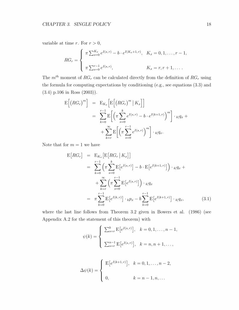
variable at time r. For r > 0,
RGr =
π
∑Kx
s=0 eI(s, r) − b · eI(Kx+1, r), Kx = 0, 1, . . . , r − 1,
π∑r−1
s=0 eI(s, r), Kx = r, r + 1, . . . .
The mth moment of RGr can be calculated directly from the definition of RGr using
the formula for computing expectations by conditioning (e.g., see equations (3.3) and
(3.4) p.106 in Ross (2003)).
E[(RGr
)m]
= EKx
[E
[(RGr
)m ∣∣Kx
]]=
r−1∑k=0
E
[(π
k∑s=0
eI(s, r) − b · eI(k+1, r))m
]· k|qx +
+∞∑
k=r
E
[(π
r−1∑s=0
eI(s, r))m
]· k|qx.
Note that for m = 1 we have
E[RGr
]= EKx
[E
[RGr
∣∣Kx
]]=
r−1∑k=0
(π
k∑s=0
E[eI(s, r)
]− b · E
[eI(k+1, r)
])· k|qx +
+∞∑
k=r
(π
r−1∑s=0
E[eI(s, r)
])· k|qx
= πr−1∑k=0
E[eI(k, r)
]· kpx − b
r−1∑k=0
E[eI(k+1, r)
]· k|qx, (3.1)
where the last line follows from Theorem 3.2 given in Bowers et al. (1986) (see
Appendix A.2 for the statement of this theorem) with
ψ(k) =
∑k
s=r E[eI(s, r)
], k = 0, 1, . . . , n− 1,
∑n−1s=r E
[eI(s, r)
], k = n, n+ 1, . . . ,
∆ψ(k) =
E
[eI(k+1, r)
], k = 0, 1, . . . , n− 2,
0, k = n− 1, n, . . .
Page 29
CHAPTER 3. SINGLE POLICY 19
and
1−G(k) = k+1px.
The prospective loss is the difference between the discounted values of future
benefits to be paid and premiums to be received. Let PLcondr be the prospective loss
random variable valued at time r and conditional on the event that the policyholder
has survived to time r.
PLcondr =
b · e−I(r, r+Jx,r+1) − π
∑r+Jx,r
s=r e−I(r, s), Jx,r = 0, 1, . . . , n− r − 1,
c · e−I(r, n) − π∑n−1
s=r e−I(r, s), Jx,r = n− r, n− r + 1, . . . ,
where Jx,r is the remaining future lifetime of (x) provided that (x) has survived to
time r. That is, {Jx,r = j} ≡ {Kx − r = j|Kx ≥ r}.
Based on the above definition of PLcondr ,
E[PLcond
r
]= EJx,r
[E
[PLcond
r
∣∣ Jx,r
]]=
n−r−1∑j=0
(b · E
[e−I(r, r+j+1)
]− π
r+j∑s=r
E[e−I(r, s)
])· j|qx+r +
+(c · E
[e−I(r, n)
]− π
n−1∑s=r
E[e−I(r, s)
])· n−rpx+r.
Alternatively, the prospective loss can be rewritten as a difference of two random
variables Z and Y, where Z represents the present value of future benefits and Y
represents the present value of future premiums of $1 valued at time r and conditional
on survival to time r. That is,
PLcondr = Z − πY, (3.2)
where
Z =
b · e−I(r, r+Jx,r+1), Jx,r = 0, 1, . . . , n− r − 1,
c · e−I(r, n), Jx,r = n− r, n− r + 1, . . . ,
Page 30
CHAPTER 3. SINGLE POLICY 20
and
Y =
∑r+Jx,r
s=r e−I(r, s), Jx,r = 0, 1, . . . , n− r − 1,
∑n−1s=r e
−I(r, s), Jx,r = n− r, n− r + 1, . . . .
Using the above definitions of Z and Y , we find that
E[Z] = EJx,r [E[Z | Jx,r]]
= bn−r−1∑
j=0
E[e−I(r,r+j+1)
]j|qx+r + c
∞∑j=n−r
E[e−I(r,n)
]j|qx+r
= bn−r−1∑
j=0
E[e−I(r,r+j+1)]
j|qx+r + cE[e−I(r,n)
]n−rpx+r
(3.3)
and
E[Y ] = EJx,r [ E[Y | Jx,r ] ]
=n−r−1∑
j=0
( r+j∑s=r
E[e−I(r,s)
])j|qx+r +
( n−1∑s=r
E[e−I(r,s)
])n−rpx+r
=n−r−1∑
j=0
E[e−I(r,r+j)
]jpx+r. (3.4)
The last line can be obtained from the theorem in Appendix A.2 with
ψ(j) =
∑r+j
s=r E[e−I(r, s)
], j = 0, 1, . . . , n− r − 1,
∑n−1s=r E
[e−I(r, s)
], j = n− r, n− r + 1, . . . ,
∆ψ(j) =
{E
[e−I(r, r+j+1)
], j = 0, 1, . . . , n− r − 2,
0, j = n− r − 1, n− r, . . .
and
1−G(j) = j+1px+r.
Page 31
CHAPTER 3. SINGLE POLICY 21
So,
E[Y ] = E[ψ(Jx,r)]
= E[e−I(r,r)
]+
n−r−2∑j=0
E[e−I(r,r+j+1)
]· j+1px+r +
∞∑j=n−r−1
0 · j+1px+r
= E[e−I(r,r)
]· 0px+r +
n−r−1∑j=1
E[e−I(r,r+j)
]· jpx+r
=n−r−1∑
j=0
E[e−I(r,r+j)
]· jpx+r. 2
Combining (3.3) and (3.4), we obtain
E[PLcondr ] = E[Z]− π E[Y ]
= bn−r−1∑
j=0
E[e−I(r,r+j+1)] j|qx+r + cE[e−I(r,n)] n−rpx+r −
− πn−r−1∑
j=0
E[e−I(r,r+j)|δ(r)] jpx+r .
The second raw moment of PLcondr is
E[(PLcond
r
)2]
=n−r−1∑
j=0
E[(b · e−I(r, r+j+1) − π
r+j∑s=r
e−I(r, s))2
]· j|qx+r +
+E[(c · e−I(r, n) − π
n−1∑s=r
e−I(r, s))2
]· n−rpx+r,
where, for example,
E[( r+j∑
s=r
e−I(r, s))2
]=
r+j∑s=r
r+j∑t=r
E[e−I(r, s)−I(r, t)
]=
r+j∑s=r
E[e−2I(r, s)
]+ 2
r+j−1∑s=r
r+j∑t=s+1
E[e−I(r, s)−I(r, t)
].
Let us now define the (unconditional) prospective loss random variable:
PLr =
{0, if Kx ≤ r − 1,
PLcondr , if Kx ≥ r.
Page 32
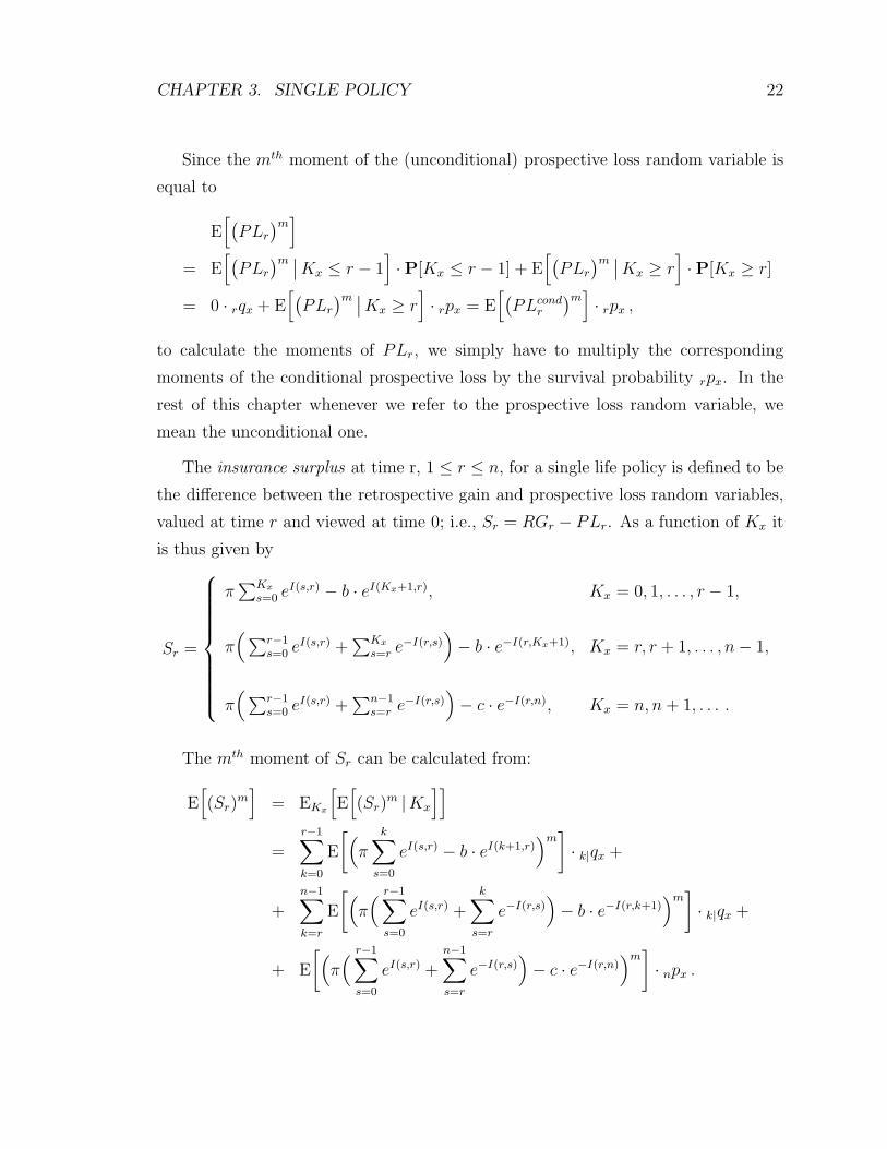
CHAPTER 3. SINGLE POLICY 22
Since the mth moment of the (unconditional) prospective loss random variable is
equal to
E[(PLr
)m]
= E[(PLr
)m ∣∣Kx ≤ r − 1]·P[Kx ≤ r − 1] + E
[(PLr
)m ∣∣Kx ≥ r]·P[Kx ≥ r]
= 0 · rqx + E[(PLr
)m ∣∣Kx ≥ r]· rpx = E
[(PLcond
r
)m]· rpx ,
to calculate the moments of PLr, we simply have to multiply the corresponding
moments of the conditional prospective loss by the survival probability rpx. In the
rest of this chapter whenever we refer to the prospective loss random variable, we
mean the unconditional one.
The insurance surplus at time r, 1 ≤ r ≤ n, for a single life policy is defined to be
the difference between the retrospective gain and prospective loss random variables,
valued at time r and viewed at time 0; i.e., Sr = RGr − PLr. As a function of Kx it
is thus given by
Sr =
π∑Kx
s=0 eI(s,r) − b · eI(Kx+1,r), Kx = 0, 1, . . . , r − 1,
π( ∑r−1
s=0 eI(s,r) +
∑Kx
s=r e−I(r,s)
)− b · e−I(r,Kx+1), Kx = r, r + 1, . . . , n− 1,
π( ∑r−1
s=0 eI(s,r) +
∑n−1s=r e
−I(r,s))− c · e−I(r,n), Kx = n, n+ 1, . . . .
The mth moment of Sr can be calculated from:
E[(Sr)
m]
= EKx
[E
[(Sr)
m |Kx
]]=
r−1∑k=0
E
[(π
k∑s=0
eI(s,r) − b · eI(k+1,r))m
]· k|qx +
+n−1∑k=r
E
[(π( r−1∑
s=0
eI(s,r) +k∑
s=r
e−I(r,s))− b · e−I(r,k+1)
)m]· k|qx +
+ E
[(π( r−1∑
s=0
eI(s,r) +n−1∑s=r
e−I(r,s))− c · e−I(r,n)
)m]· npx .
Page 33
CHAPTER 3. SINGLE POLICY 23
3.2 Numerical Illustrations
Consider a single life policy with $1000 benefit issued to a person aged 30. The
premium for this policy is determined according to the equivalence principle (see
Appendix A.4 for more details on the equivalence principle). The results derived
in the previous section are illustrated for the temporary and endowment insurance
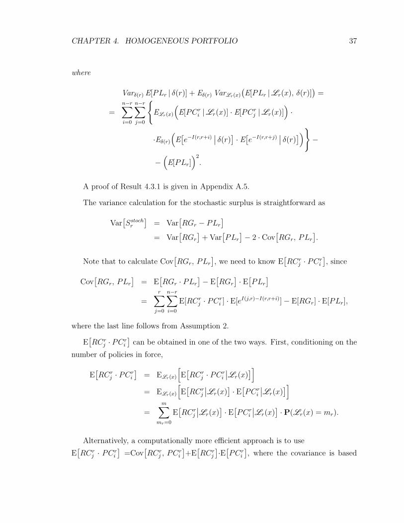
contracts with the term equal to 5 years (see Tables 3.1 and 3.2), 10 years (see
Figure 3.1) and 25 years (see Figure 3.2).
We begin by analyzing the behaviour of the expected values of the retrospective
gain, prospective loss and surplus conditional on the force of interest at time r; the
values for three possible realizations of δ(r) (4%, 6% - the long-term mean of the
process and 8% - the starting value of the process) are given in the middle three
columns of Tables 3.1 and 3.2. Observe that when δr decreases, the conditional
expected values of RGr decrease but the conditional expected values of PLr increase.
This is due to the effects of accumulating and discounting at lower rates of return.
Since Sr = RGr − PLr, the expected value of the surplus decreases by the amount
equal to the sum of the gain decrease and the loss increase.
Comparing the unconditional expected values of the retrospective gain and prospec-
tive loss, we can see that, for the temporary insurance contracts, the expected values
at first rise but then begin to decline as r approaches the term of the contract, which
is clearly demonstrated in the upper left panels of Figures 3.1 and 3.2. This is consis-
tent with building up a small reserve in early years of the contract and then spending
it since no benefit has to be paid under the terms of this contract if a policyholder
survives up to the contract maturity. In the case of the endowment contracts, the
expected values gradually increase to the amount of the benefit, which would have
to be paid with certainty at time n if the policy is in force at time (n− 1) (death in
year n would result in the death benefit payment and survival to time n would result
in the pure endowment benefit).
We can also observe that the expected value of the surplus increases with r. Even
though in these examples pricing of the contracts is done according to the equivalence
principle, the mean value of the surplus is positive at all valuation dates we considered.
This can be attributed to the Gaussian nature of the rates of return. The asymmetry
Page 34
CHAPTER 3. SINGLE POLICY 24
of the process with nonzero variance results in a larger accumulation effect compared
to the discounting effect. If the variance of the process was zero or, in other words, if
the rates of return were deterministic, then an accumulation factor would be exactly
the inverse of the corresponding discount factor. But in the environment of stochastic
rates of return the product of the expected values of the accumulation and discount
factors is always greater than one:
E[eI(s,r)
]· E
[e−I(s,r)
]= eE[I(s,r)]+ 1
2Var[I(s,r)] · e−E[I(s,r)]+ 1
2Var[I(s,r)]
= eVar[I(s,r)] > 1 if Var[I(s, r)] > 0.
As r increases, so does the variability of the retrospective gain, since there is both
a larger uncertainty about future cash flows and rates of return. Note that in general
the variability of the prospective loss depends on the number of deaths up to time r,
the death pattern after time r and the randomness of the future rates of return. The
combination of these three factors may cause the overall variability to either increase
or decrease with r depending on the relative importance of each of them. For the
contracts we considered the behaviour of the standard deviation of PLr varies with
the type and the term of the contract. For the 5-year and 10-year temporary policies,
the prospective loss becomes less volatile for larger values of r; for the 25-year policy,
the standard deviation slightly increases initially and then declines. This decline in
the variability for larger values of r is due to a smaller uncertainty about the death
pattern after time r and the fact that the mortality component of temporary policies
usually dominates the investment one. The standard deviation of the prospective loss
for endowment policies at first declines but then increases for values of r approaching
the term of the contract. In the case of endowment policies, it is the increase in
the uncertainty about future rates of return that drives the overall variability of the
prospective loss up for larger values of r.
Page 35
CHAPTER 3. SINGLE POLICY 25
δr: .04 .06 .08r E[RGr|δ(r) = δr] E[RGr]1 0.0209 0.0475 0.0748 0.07212 0.0504 0.0923 0.1356 0.12753 0.0425 0.1007 0.1612 0.14534 -0.0142 0.0603 0.1387 0.1128r E[PLr|δ(r) = δr] E[PLr]1 0.2259 0.1422 0.0633 0.07162 0.2452 0.1777 0.1133 0.12603 0.2236 0.1757 0.1295 0.14234 0.1493 0.1241 0.0994 0.1080r E[Sr|δ(r) = δr] E[Sr]1 -0.2051 -0.0947 0.0115 0.00052 -0.1948 -0.0854 0.0222 0.00153 -0.1811 -0.0751 0.0317 0.00304 -0.1635 -0.0638 0.0393 0.0048
r SD[RGr|δ(r) = δr] SD[RGr]1 36.0321 36.0321 36.0321 36.03212 52.1823 52.7301 53.2943 53.19103 65.9218 67.1683 68.4635 68.13084 78.7362 80.8513 83.0687 82.3566r SD[PLr|δ(r) = δr] SD[PLr]1 66.8353 64.2498 61.7977 62.06452 59.6696 57.7330 55.8769 56.25463 50.2845 49.0007 47.7559 48.11104 36.7656 36.1097 35.4655 35.6944r SD[Sr|δ(r) = δr] SD[Sr]1 75.9255 73.6613 71.5339 71.76442 79.2600 78.1831 77.2133 77.41563 82.8997 83.1334 83.4672 83.39824 86.8871 88.5402 90.3162 89.7519
Table 3.1: Expected values and standard deviations of retrospective gain, prospectiveloss and surplus for 5-year temporary insurance contract.
Page 36
CHAPTER 3. SINGLE POLICY 26
δr: .04 .06 .08r E[RGr|δ(r) = δr] E[RGr]1 165.4803 168.8495 172.2867 171.94852 340.9904 349.7112 358.6631 356.99763 525.9515 542.8011 560.2265 555.62834 720.9330 748.9411 778.1309 768.4117r E[PLr|δ(r) = δr] E[PLr]1 237.4258 201.5997 168.2494 171.76912 416.2425 382.2705 350.0646 356.43553 601.9631 573.9670 546.9549 554.47564 794.3808 777.3667 760.6562 766.4814r E[Sr|δ(r) = δr] E[Sr]1 -71.9455 -32.7502 4.0374 0.17942 -75.2521 -32.5593 8.5985 0.56223 -76.0116 -31.1659 13.2717 1.15274 -73.4478 -28.4257 17.4747 1.9303
r SD[RGr|δ(r) = δr] SD[RGr]1 36.0321 36.0321 36.0321 36.07372 56.6342 57.3125 58.0101 58.20013 77.2717 78.9073 80.6023 81.34514 99.2467 102.1808 105.2453 107.3234r SD[PLr|δ(r) = δr] SD[PLr]1 42.0424 40.6415 39.4018 42.73682 37.2222 35.6113 34.1390 40.51803 42.8343 41.0689 39.3771 45.08674 59.1968 57.9345 56.6947 58.9303r SD[Sr|δ(r) = δr] SD[Sr]1 49.4829 49.2533 49.1260 52.31922 46.7823 48.1719 49.6357 56.46643 44.7365 47.6706 50.6774 60.88354 44.9518 49.1162 53.4076 65.6090
Table 3.2: Expected values and standard deviations of retrospective gain, prospectiveloss and surplus for 5-year endowment insurance contract.
Page 37
CHAPTER 3. SINGLE POLICY 27
●
●
●
●
● ●●
●
●
0 2 4 6 8 10
0.2
0.3
0.4
0.5
0.6
10−year temporary insurance
r
Exp
ecte
d V
alue
10−year temporary insurance
● Retrospective Gain
Prospective Loss
●
●
●
●
●
●
●
●
●
0 2 4 6 8 10
4060
8010
012
014
016
0
10−year temporary insurance
r
Sta
ndar
d D
evia
tion
● Retrospective Gain
Prospective Loss
Surplus
●
●
●
●
●
●
●
●
●
0 2 4 6 8 10
200
400
600
800
10−year endowment insurance
r
Exp
ecte
d V
alue
● Retrospective Gain
Prospective Loss
●
●
●
●
●
●
●
●
●
0 2 4 6 8 10
5010
015
020
0
10−year endowment insurance
r
Sta
ndar
d D
evia
tion
● Retrospective Gain
Prospective Loss
Surplus
Figure 3.1: Expected values and standard deviations of retrospective gain, prospectiveloss and surplus for 10-year temporary and endowment contracts.
Page 38
CHAPTER 3. SINGLE POLICY 28
●
●
●
●
●
●
●
●
●
●
●
●
●
●
●
●● ●
●
●
●
●
●
●
0 5 10 15 20 25
510
1525−year temporary insurance
r
Exp
ecte
d V
alue
25−year temporary insurance
● Retrospective Gain
Prospective Loss
●
●
●
●
●
●
●
●
●
●
●
●
●
●
●
●
●
●
●
●
●
●
●
●
0 5 10 15 20 25
100
200
300
400
500
25−year temporary insurance
r
Sta
ndar
d D
evia
tion
● Retrospective Gain
Prospective Loss
Surplus
●●
●●
●
●
●
●
●
●
●
●
●
●
●
●
●
●
●
●
●
●
●
●
0 5 10 15 20 25
020
040
060
080
0
25−year endowment insurance
r
Exp
ecte
d V
alue
● Retrospective Gain
Prospective Loss
●
●
●●
●
●
●
●
●
●
●
●
●
●
●
●
●
●
●
●
●
●
●
●
0 5 10 15 20 25
100
200
300
400
500
600
700
25−year endowment insurance
r
Sta
ndar
d D
evia
tion
● Retrospective Gain
Prospective Loss
Surplus
Figure 3.2: Expected values and standard deviations of retrospective gain, prospectiveloss and surplus for 25-year temporary and endowment contracts.
Page 39
Chapter 4
Portfolio of Homogeneous Life
Insurance Policies
In practice, insurers deal not with just one insurance policy but rather with a col-
lection of policies forming an insurance portfolio. Therefore, our next objective is
to extend the results for one insurance contract developed in the previous chapter to
study portfolios of insurance contracts. One way to proceed is to define the retrospec-
tive gain, prospective loss and surplus for a portfolio by aggregating the corresponding
random variables for one policy over the number of policies in the portfolio. However,
for large portfolios, say 100,000 policies, this approach might not be very efficient.
Alternatively, we could model portfolio’s cash flows in every year, in which case the
maximum number of terms to add up is equal to the duration of the policies in the
portfolio. This is the approach we will adopt.
Consider a portfolio of identical life policies issued to a group of m policyholders
all aged x with the same mortality profile. Similar to a single policy discussed in
the previous chapter, each contract pays a death benefit b at the end of the year of
death if death occurs within n years and a pure endowment benefit c if a policyholder
survives to the end of year n. π is the annual level premium payable at the beginning
of each year as long as the contract remains in force. This portfolio is referred to as
being homogeneous.
29
Page 40
CHAPTER 4. HOMOGENEOUS PORTFOLIO 30
4.1 Retrospective Gain
Let RCrj denote the net cash flow at time j prior to time r, 0 ≤ j ≤ r (i.e., it is a
retrospective cash flow for valuation at time r).
RCrj =
m∑i=1
[π ·Li,j(x) · 1{j<r} − b ·Di,j(x) · 1{j>0}
]= π ·
( m∑i=1
Li,j(x)
)· 1{j<r} − b ·
( m∑i=1
Di,j(x)
)· 1{j>0}
= π ·Lj(x) · 1{j<r} − b ·Dj(x) · 1{j>0} , (4.1)
where
Li,j(x) =
{1 if policyholder i aged x survives for j years,
0 otherwise,
Di,j(x) =
{1 if policyholder i aged x dies in year [j − 1, j),
0 otherwise,
and 1{A} is an indicator; it is equal to 1 if condition A is true and 0 otherwise.
Indicator 1{j>0} multiplying the second term in Equation (4.1) reinforces the fact
that no death benefit is paid at the beginning of the first year of the contract (i.e.,
when j = 0). So, RCr0 is the sum of all the premiums collected at the issue date. Now
consider what happens at time j = r. Death benefits are paid at the end of year r
to everyone who dies during that year. So, this cash outflow becomes a part of the
retrospective cash flow RCrr . However, premiums are collected at the beginning of the
next year ((r + 1)st year) and therefore they contribute to the prospective cash flow
(more formally defined in the next section). This is why indicator 1{j<r} multiplies
the first term in Equation (4.1), which makes the premiums inflow disappear for j = r.
Lj(x) =∑m
i=1 Li,j(x) denotes the number of people from the initial group of m
policyholders aged x who survive to time j (i.e. it is the number of inforce policies
at time j) and Dj(x) =∑m
i=1 Di,j(x) denotes the number of deaths in year [j − 1, j).
Observe that Lj(x) and Dj(x) have binomial distributions with
Lj(x) ∼BIN(m, jpx) and Dj(x) ∼BIN(m, j−1|qx).
Page 41
CHAPTER 4. HOMOGENEOUS PORTFOLIO 31
This can be used to calculate
E[RCrj ] = π · E[Lj(x)] · 1{j<r} − b · E[Dj(x)] · 1{j>0}
= π · (m · jpx) · 1{j<r} − b · (m · j−1|qx) · 1{j>0} ,
Var[RCrj ] = π2 · Var(Lj(x)) · 1{j<r} + b2 · Var(Dj(x)) · 1{j>0} −
− 2 · π · b · Cov(Lj(x),Dj(x)) · 1{0<j<r}
and, for i < j,
Cov[RCri , RC
rj ] = π2 · Cov[Li(x),Lj(x)] · 1{j<r} + b2 · Cov[Di(x),Dj(x)] · 1{i>0}
− π · b · Cov[Li(x),Dj(x)] · 1{0<i<j<r}
− b · π · Cov[Di(x),Lj(x)] · 1{0≤i<j≤r} .
The covariance between cash flows arises due to the fact that, if a person belongs
to Li(x) (i.e., he or she was alive at time i), the same person might also belong to
either Lj(x) or Dj(x) at some later time j > i. For different policyholders, it was
assumed earlier that their lifetimes are independent (Assumption 1).
The formulas for various variance and covariance terms used above are given in
the next section; see Equations (4.6)-(4.12) with r set to zero and L0(x) equal to m.
The retrospective gain at a given time r is equal to the accumulated value to time
r of all net cash flows that occur prior to that time. So, using the cash flow approach,
we can express the retrospective gain in terms of RCrj as follows:
RGr =∑r
j=0RCrj · eI(j,r).
Then, under Assumption 2 (i.e., assuming independence between future lifetimes
and interest rates) we obtain
E[RGr] =r∑
j=0
E[RCrj ] · E[eI(j,r)] (4.2)
and
E[(RGr
)2]
=r∑
i=0
r∑j=0
E[RCri ·RCr
j ] · E[eI(i,r)+I(j,r)]. (4.3)
Page 42
CHAPTER 4. HOMOGENEOUS PORTFOLIO 32
One might also be interested in the retrospective gain random variable conditional
on the force of interest at time r and/or the number of policies remaining in the
portfolio at that time. This allows to further investigate properties of RGr with
respect to changes in rates of return and the mortality experience of the portfolio
by considering various scenarios. Appendix A.3 provides details on how to calculate
the expected value, variance and covariance of retrospective cash flows conditional
on the size of the portfolio at a particular valuation date. These results, combined
with conditional moments of the accumulation function, can then be used to calculate
E[RGr
∣∣ Lr(x), δ(r)]
and E[(RGr
)2∣∣ Lr(x), δ(r)]
as follows:
E[RGr |Lr(x), δ(r)] =r∑
j=0
E[RCrj |Lr(x)] · E[eI(j,r) | δ(r)] (4.4)
and
E[(RGr
)2]
=r∑
i=0
r∑j=0
E[RCri ·RCr
j |Lr(x)] · E[eI(i,r)+I(j,r) | δ(r)]. (4.5)
4.2 Prospective Loss
Similar to RCrj defined in the previous section to study the retrospective gain RGr, we
let PCrj denote the net cash flow that occurs j time units after time r, 0 ≤ j ≤ n− r,
(i.e., it is the prospective cash flow for valuation at time r), which will be used to
study the prospective loss random variable, PLr.
Since we want to express a prospective loss in terms of PCrj , a prospective cash
flow at any given time j is the difference between benefits paid and premiums collected
at that time. Using the notation introduced in the previous section, we have
PCrj =
mr∑i=1
[b ·Di,j(x+ r) · 1{j>0} + c ·Li,(n−r)(x+ r) · 1{j=n−r} −
− π ·Li,j(x+ r) · 1{j<n−r}]
= b ·( mr∑
i=1
Di,j(x+ r))· 1{j>0} + c ·
( mr∑i=1
Li,(n−r)(x+ r))· 1{j=n−r}
− π ·( mr∑
i=1
Li,j(x+ r))· 1{j<n−r}
= b ·Dj(x+ r) · 1{j>0} + c ·Ln−r(x+ r) · 1{j=n−r} − π ·Lj(x+ r) · 1{j<n−r},
Page 43
CHAPTER 4. HOMOGENEOUS PORTFOLIO 33
where mr is the size of the portfolio at time r (i.e., the realization of Lr(x)).
Since for 0 < j ≤ n− r
{Lj(x+ r)|Lr(x) = mr} ∼ BIN(mr, jpx+r) and
{Dj(x+ r)|Lr(x) = mr} ∼ BIN(mr, j−1|qx+r) ,
we can use the known moments of binomially distributed random variables to find
the moments of PCrj , which are 1
E[PCrj |Lr] = b · E[Dj(x+ r)|Lr] · 1{j>0} + c · E[Ln−r(x+ r)|Lr] · 1{j=n−r}
− π · E[Lj(x+ r)|Lr] · 1{j<n−r}
= b ·(Lr · j−1|qx+r
)· 1{j>0} + c ·
(Lr · jpx+r
)· 1{j=n−r}
− π ·(Lr · jpx+r
)· 1{j<n−r}
and
Var[PCrj |Lr] = b2 · Var[Dj(x+ r)|Lr] · 1{j>0}
+ c2 · Var[Ln−r(x+ r)|Lr] · 1{j=n−r}
+ π2 · Var[Lj(x+ r)|Lr] · 1{j<n−r}
+ 2 · b · c · Cov[Dj(x+ r),Lj(x+ r)|Lr] · 1{j=n−r}
− 2 · b · π · Cov[Dj(x+ r),Lj(x+ r)|Lr] · 1{0<j<n−r} .
For 0 ≤ i < j ≤ n− r,
Cov[PCrj , PC
ri |Lr] = b2 · Cov[Dj(x+ r), Di(x+ r) |Lr] · 1{i>0}
+ π2 · Cov[Lj(x+ r), Li(x+ r) |Lr] · 1{j<n−r}
+ c · b · Cov[Lj(x+ r), Di(x+ r) |Lr] · 1{0<i<j=n−r}
− b · π · Cov[Dj(x+ r), Li(x+ r) |Lr] · 1{0≤i<j≤n−r}
− π · b · Cov[Lj(x+ r), Di(x+ r) |Lr] · 1{0<i<j<n−r}
− c · π · Cov[Lj(x+ r), Li(x+ r) |Lr] · 1{j=n−r},
1For simplicity of notation, in some cases we will use Lr instead of Lr(x) when there is noambiguity about age x.
Page 44
CHAPTER 4. HOMOGENEOUS PORTFOLIO 34
where
Var[Lj(x+ r) |Lr] = Lr · jpx+r · (1− jpx+r); (4.6)
Var[Dj(x+ r) |Lr] = Lr · j−1|qx+r · (1− j−1qx+r); (4.7)
Cov[Dj(x+ r), Lj(x+ r) |Lr] = −Lr · j−1|qx+r · jpx+r; (4.8)
Cov[Dj(x+ r), Di(x+ r) |Lr] = −Lr · j−1|qx+r · i−1|qx+r; (4.9)
Cov[Lj(x+ r), Li(x+ r) |Lr] = Lr · (jpx+r − ipx+r · jpx+r); (4.10)
Cov[Dj(x+ r), Li(x+ r) |Lr] = Lr · j−1|qx+r · (1− ipx+r); (4.11)
Cov[Lj(x+ r), Di(x+ r) |Lr] = −Lr · jpx+r · i−1|qx+r. (4.12)
Now we can rewrite PLr in terms of PCrj and calculate its first two raw moments
using the results developed above. We get
PLr =n−r∑j=0
PCrj · e−I(r,r+j), (4.13)
E[PLr |Lr, δ(r)] =n−r∑j=0
E[PCrj |Lr] · E[e−I(r,r+j) | δ(r)] (4.14)
and
E[(PLr)2 |Lr, δ(r)] =
n−r∑i=0
n−r∑j=0
(E[PCr
i · PCrj |Lr] · E[e−I(r,r+i)−I(r,r+j) | δ(r)]
)=
n−r∑j=0
(E[(PCr
j )2 |Lr] · E[e−2I(r,r+j) | δ(r)]
)+
+ 2 ·n−r−1∑
i=0
n−r∑j=i+1
(E[PCr
i · PCrj |Lr] · E[e−I(r,r+i)−I(r,r+j) | δ(r)]
), (4.15)
since {K(i)x } are independent of {δ(j), j = 0, 1, . . .} (Assumption 2).
We can calculate E[PLr] and Var[PLr] either using Equations (4.14) and (4.15)
and taking double expectations over Lr(x) and δ(r), or directly from Equation (4.13).
Page 45
CHAPTER 4. HOMOGENEOUS PORTFOLIO 35
4.3 Insurance Surplus
4.3.1 Introduction
In general, we define insurance surplus to be the difference between assets and liabil-
ities at a given valuation date. Recall that the retrospective gain is the accumulated
value of past premiums collected net of past benefits paid and, thus, in our context, it
can be viewed as the value of assets. In turn, the liabilities associated with a portfolio
of life policies are based on the prospective loss, which is the discounted value of fu-
ture obligations net of future premiums. So, the liabilities can simply be represented
by the prospective loss random variable. In this case the surplus is referred to as the
net stochastic surplus or just stochastic surplus and is denoted Sstochr .
In practice, at each valuation date, an insurer is required to set aside an actuarial
reserve based on the number of policies in force as well as on the current interest rate.
This reserve is a liability item on the balance sheet of the insurance company. So, an
alternative definition of the surplus is the difference between the value of assets and
the actuarial reserve, in which case we call it the accounting surplus and denote it
Sacctr .
The reserve is intended to cover the future liabilities of the insurer. Therefore,
the amount needed to be set as a reserve at time r should be at least the expected
value of PLr conditional on the number of inforce policies in the portfolio Lr(x) and
the force of interest δ(r). If, instead, it is required to have a conservative reserve that
will cover net future obligations with a high probability, one can use a pth percentile
of the prospective loss random variable with p between 70% and 95%, for example.
However, this reserve can be fairly difficult to incorporate in the model, since we need
to know the distribution function of PLr, which is not easy to obtain. Alternatively,
a reserve could be set equal to the expected value plus a multiple of the standard
deviation of PLr (see Norberg (1993)).
In the rest of this section we derive the first two moments of the stochastic and
accounting surpluses, assuming that the reserve is given by the conditional expected
value of the prospective loss random variable.
Page 46
CHAPTER 4. HOMOGENEOUS PORTFOLIO 36
4.3.2 Methodology
Let rV (Lr(x), δ(r)) or simply rV denote the reserve at time r. It is a function of
Lr(x) and δ(r) and thus, when viewed from time 0, is a random quantity whose value
at time r depends on the realizations of Lr(x) and δ(r).
{Sacctr |Lr(x), δ(r)} = {RGr|Lr(x), δ(r)} − rV (Lr(x), δ(r)) (4.16)
is the accounting surplus at time r conditional on the number of policies in force and
the force of interest at that time.
The stochastic surplus is given by
Sstochr = RGr − PLr . (4.17)
Assume that
rV ≡ rV (Lr(x), δ(r)) = E[PLr |Lr, δ(r)
]. (4.18)
We then have
E[Sacctr ] = Eδ(r)
[ELr
[E
[Sacct
r |Lr, δ(r)]]]
= Eδ(r)
[ELr
[E
[RGr |Lr, δ(r)
]]]− Eδ(r)
[ELr
[E
[PLr |Lr, δ(r)
]]]= E[RGr]− E[PLr]
= E[RGr − PLr]
= E[Sstochr ].
That is, with our particular choice of the reserve, stochastic and accounting surpluses
have the same expected value.
Let us next consider the variance of the accounting surplus when the reserve is
given by Equation (4.18).
Result 4.3.1.
Var[Sacctr ] =
(Varδ(r) E[PLr | δ(r)] + Eδ(r) VarLr(x)
(E[PLr |Lr(x), δ(r)]
))+Var[RGr]− 2Cov(RGr, PLr),
Page 47
CHAPTER 4. HOMOGENEOUS PORTFOLIO 37
where
Varδ(r) E[PLr | δ(r)] + Eδ(r) VarLr(x)
(E[PLr |Lr(x), δ(r)]
)=
=n−r∑i=0
n−r∑j=0
{ELr(x)
(E[PCr
i |Lr(x)] · E[PCrj |Lr(x)]
)·
·Eδ(r)
(E[e−I(r,r+i)
∣∣ δ(r)] · E[e−I(r,r+j)
∣∣ δ(r)])}−
−(E[PLr]
)2
.
A proof of Result 4.3.1 is given in Appendix A.5.
The variance calculation for the stochastic surplus is straightforward as
Var[Sstoch
r
]= Var
[RGr − PLr
]= Var
[RGr
]+ Var
[PLr
]− 2 · Cov
[RGr, PLr
].
Note that to calculate Cov[RGr, PLr
], we need to know E
[RCr
j · PCri
], since
Cov[RGr, PLr
]= E
[RGr · PLr
]− E
[RGr
]· E
[PLr
]=
r∑j=0
n−r∑i=0
E[RCrj · PCr
i ] · E[eI(j,r)−I(r,r+i)]− E[RGr] · E[PLr],
where the last line follows from Assumption 2.
E[RCr
j · PCri
]can be obtained in one of the two ways. First, conditioning on the
number of policies in force,
E[RCr
j · PCri
]= ELr(x)
[E
[RCr
j · PCri
∣∣Lr(x)]]
= ELr(x)
[E
[RCr
j
∣∣Lr(x)]· E
[PCr
i
∣∣Lr(x)]]
=m∑
mr=0
E[RCr
j
∣∣Lr(x)]· E
[PCr
i
∣∣Lr(x)]·P(Lr(x) = mr).
Alternatively, a computationally more efficient approach is to use
E[RCr
j · PCri
]=Cov
[RCr
j , PCri
]+E
[RCr
j
]·E
[PCr
i
], where the covariance is based
Page 48
CHAPTER 4. HOMOGENEOUS PORTFOLIO 38
directly on the definitions of RCrj and PCr
i .
Cov[RCr
j , PCri
]= π · b · Cov
[Lj(x), Di(x+ r)
]· 1{j<r, i>0}
+ π · c · Cov[Lj(x), Li(x+ r)
]· 1{j<r, i=n−r, i>0}
− π2 · Cov[Lj(x), Li(x+ r)
]· 1{j<r, i<n−r}
− b2 · Cov[Dj(x), Di(x+ r)
]· 1{j>0, i>0}
− b · c · Cov[Dj(x), Li(x+ r)
]· 1{j>0, i=n−r, i>0}
+ b · π · Cov[Dj(x), Li(x+ r)
]· 1{j>0, i<n−r} ,
where
Cov[Lj(x), Di(x+ r)
]= m · (r+i−1|qx − jpx · r+i−1|qx)
= m · r+i−1|qx · (1− jpx) ,
Cov[Lj(x), Li(x+ r)
]= m · (r+ipx − jpx · r+ipx)
= m · r+ipx · (1− jpx) ,
Cov[Dj(x), Di(x+ r)
]= −m · j−1|qx · r+i−1|qx and
Cov[Dj(x), Li(x+ r)
]= −m · j−1|qx · r+ipx.
4.4 A Note on Variance for Limiting Portfolio
A limiting portfolio is an abstract concept and is not achievable in practice. However,
its characteristics such as variability can serve as benchmarks for portfolios of finite
sizes and can provide some useful information for insurance risk managers.
If the variance of the surplus per policy for a given portfolio is much larger than
the corresponding variance for the limiting portfolio, then it can be concluded that
a large portion of the total risk is due to the insurance risk. In other words, there
is a great uncertainty about future cash flows. One implication of this is that, if
the insurer decides to hedge the financial risk, for instance, by purchasing bonds
Page 49
CHAPTER 4. HOMOGENEOUS PORTFOLIO 39
whose cash flows will match those of the portfolio’s liabilities, this strategy will not
be very efficient and the cost incurred to implement it might not be justified. In this
case, selling more policies, sharing the mortality risk or buying reinsurance are better
strategies to mitigate the risk.
For a limiting portfolio, the calculation of the moments is done similarly to the
case when the size of the portfolio is finite, except that the random cash flows per
policy, RCrj /m and PCr
i /m, are replaced by their expected values. For example, the
second raw moment of RGr/m and PLr/m and the covariance between them become
limm→∞
E[(RGr/m
)2]
=r∑
i=0
r∑j=0
E[RCri /m] · E[RCr
j /m] · E[eI(i,r)+I(j,r)],
limm→∞
E[(PLr/m
)2]
=n−r∑i=0
n−r∑j=0
E[PCri /m] · E[PCr
j /m] · E[e−I(r,r+i)−I(r,r+j)]
and
limm→∞
Cov(RGr/m, PLr/m
)=
r∑j=0
n−r∑i=0
E[RCrj /m] · E[PCr
i /m] · Cov(eI(j,r), e−I(r,r+i)
).
4.5 Numerical Illustrations
Consider homogeneous portfolios of life policies with $1000 benefit issued to people
aged 30 and with premiums determined under the equivalence principle (see Ap-
pendix A.4). Note that the expected values of the retrospective gain and prospective
loss per policy as well as the two types of surplus 2 per policy are the same as for a
single policy which we discussed in the previous chapter. Here, we would like to see
how the riskiness of the portfolio, as measured by the standard deviation, changes
with respect to changes in the initial portfolio size. The results are presented for
portfolios of size 100, 10,000, 100,000 and the infinite size (limiting portfolio). To
compare portfolios of different sizes, all quantities are calculated on the per policy
basis.
2This is true for the accounting surplus only with our particular choice of the reserve equal tothe expected value of the prospective loss.
Page 50
CHAPTER 4. HOMOGENEOUS PORTFOLIO 40
Tables 4.1 and 4.2 give standard deviations of the retrospective gain at time r per
policy conditional on the force of interest δ(r) for the portfolios of 5-year temporary
and 5-year endowment insurance contracts respectively. Three scenarios of possible
realizations of δ(r) (4%, 6% and 8%) are considered. Comparing the standard devia-
tions for portfolios of different sizes, we see that they decrease as m increases. This is
due to the diversification of the mortality risk. However, notice that this effect is much
larger for portfolios of temporary policies than for portfolios of endowment policies.
For example, in the case of temporary insurances when m = 10, 000, SD[RG1/m] is
almost 8 times larger than SD[RG1/m] for the limiting portfolio (0.1148 vs. 0.0137)
and at r = 4 the ratio is almost 3.5 (.2721 vs. 0.0788). But for portfolios of endow-
ment insurances, even when there are only 100 policies, the ratio is around 2 at r = 1
(3.9981 vs. 1.7325) and just over 1 at r = 4 (29.1919 vs. 27.2842). Increasing the
size of the portfolio of endowment contracts to 10,000 almost entirely eliminates the
insurance risk.
This can be explained by the relative size of the mortality and investment risks.
For short term (such as 5 years) temporary policies most of the risk comes from
the uncertainty about how many deaths occurs during the duration of the contract.
Therefore, for a small portfolio, when the size of the portfolio increases by a factor
of, say, 100, one would expect the standard deviation to go down by a factor of
about 10 (the square root of 100). We can see that for m increasing from 1 to
100 and from 100 to 10,000. But an endowment policy is essentially an investment
product that pays the benefit at the end of the term with a very high probability
(e.g., probability that a 30 year old male survives for 5 years is 0.9931488, which is the
probability of paying the pure endowment benefit) and so the small mortality risk gets
quickly diversified for portfolios of even moderate size leaving only the nondiversifiable
investment risk. Another way to see this is to compare conditional standard deviations
to the corresponding unconditional ones. In the case of temporary contracts, there
is a fairly small difference between them (e.g., for m = 10, 000, SD[RG4/m] and
SD[RG4/m | δ(4)] are all around 0.8), but in the case of endowment contracts, for
some parameters, unconditional standard deviations are almost three times as large
(e.g., for m = 10, 000, SD[RG4/m]=27.3 vs. SD[RG4/m | δ(4)] ≈ 9.6). We can
see that unconditional standard deviations are always larger than the corresponding
Page 51
CHAPTER 4. HOMOGENEOUS PORTFOLIO 41
conditional ones confirming the conditional variance formula
Var(RGr/m
)= Var
(E
[RGr/m | δ(r)
])+ E
(Var
[RGr/m | δ(r)
]).
Also, note that the conditional standard deviations for the limiting portfolios at r = 1
are equal to zero due to the absence of the investment risk in our model and a full
diversification of the insurance risk. Hence, the corresponding unconditional deviation
represents pure investment risk at time r = 1.
Results for the prospective loss random variable, similar to those presented in
Tables 4.1 and 4.2, are summarized in Tables 4.3 and 4.4.
Tables 4.5, 4.6, 4.7 and 4.8 give standard deviations of the accounting and stochas-
tic surpluses for portfolios of 5-year temporary and 5-year endowment insurance poli-
cies. Table 4.9 shows correlation coefficients between retrospective gain and prospec-
tive loss random variables for portfolios of 5-year endowment policies.
Observe that as r increases, so do the conditional and unconditional standard
deviations of the accounting surplus. For the stochastic surplus, although there is a
reduction in the variability of the prospective loss for larger r, it might or might not
be sufficient to offset an increase in the uncertainty of the retrospective gain.
Comparing standard deviations corresponding to the same r but for different
values of m, we can see that as m increases, there is a reduction in variability of the
accounting surplus. As we already noted above, this reduction is attributed to the
diversification of the mortality risk. However, even in the limiting case of endowment
contracts, variability does not reduce to zero, since investment risk is nondiversifiable
and remains present regardless of the size of the portfolio.
It is interesting to note that the standard deviation of the stochastic surplus at
valuation dates close to maturity for portfolios of endowment policies increases for
larger portfolio sizes. Recall that
Var[Sstoch
r /m]
= Var[RGr/m
]+ Var
[PLr/m
]− 2 · Cov
[RGr/m, PLr/m
].
We saw that the variability of both retrospective gain and prospective loss per policy
random variables decreases as m increases. This suggests that the increase comes
from the covariance component, which has to decrease to make Var[Sstoch
r /m]
larger
Page 52
CHAPTER 4. HOMOGENEOUS PORTFOLIO 42
because of the minus sign. By looking at the correlation coefficients between RGr/m
and PLr/m, both conditional and unconditional, we can see that as m increases the
correlation coefficients decrease. At earlier valuation dates, decrease in the variabil-
ity of RGr/m and PLr/m seems to be sufficient to compensate for decrease in the
covariance, but eventually, for r close to n, the reduction in the covariance slightly
outweighs reduction in the variances of RGr/m and PLr/m.
It is easy to see from Figure 4.1 that the stochastic surplus is more volatile than the
accounting surplus. In the former case, the uncertainty in liabilities arises from the
uncertainty in the complete future path of rates of return and mortality experience;
whereas in the latter case, the randomness of liabilities comes from the uncertainty
in the number of inforce policies remaining in the portfolio and the rate of return at
the valuation date only.
Also notice that as r increases, the difference in the volatilities of stochastic and
accounting surpluses diminishes. In fact, at r equal to n (the term of the contract),
conditional on the number of policyholders who survive to time n, there is no uncer-
tainty about the liabilities and all the variation comes from the retrospective gain,
which represents the asset side and is the same for the stochastic and accounting
surpluses.
Figures 4.2 and 4.3 display the standard deviations of accounting and stochastic
surpluses per policy conditional on the number of inforce policies at time r (referred
to as ’inforce size’ on the axes labels), Lr(x), and the force of interest in year r,
δ(r), plotted against possible realizations of Lr(x) and δ(r). The plots are shown for
portfolios of 100 10-year temporary and 10-year endowment life insurance policies at
r equal to 5 and 8. For the portfolio of temporary policies, observe a steep increase
in the variability of the accounting surplus when the inforce size decreases from 100
policies to 99 policies and a less rapid increase for further decreases in the inforce
size. The shape of these plots is difficult to explain because of the different factors
affecting the variability of the surplus. One would expect the variability to be high
when the probability of death in the time interval from 0 to r is about 0.5 and when
the variability of the accumulation and discounting factors is high.
Page 53
CHAPTER 4. HOMOGENEOUS PORTFOLIO 43
δr: .04 .06 .08m=1
r SD[RGr/m|δ(r) = δr] SD[RGr/m]1 36.0321 36.0321 36.0321 36.03212 52.1823 52.7301 53.2943 53.19103 65.9218 67.1683 68.4635 68.13084 78.7362 80.8513 83.0687 82.3566
m=100r SD[RGr/m|δ(r) = δr] SD[RGr/m]1 3.6032 3.6032 3.6032 3.60322 5.2182 5.2730 5.3294 5.31923 6.5922 6.7169 6.8464 6.81334 7.8737 8.0852 8.3070 8.2360
m=10,000r SD[RGr/m|δ(r) = δr] SD[RGr/m]1 0.3631 0.3631 0.3631 0.36332 0.5295 0.5352 0.5411 0.53613 0.6725 0.6856 0.6992 0.68754 0.8088 0.8312 0.8546 0.8345
m=100,000r SD[RGr/m|δ(r) = δr] SD[RGr/m]1 0.1139 0.1139 0.1139 0.11482 0.1653 0.1671 0.1689 0.17113 0.2096 0.2136 0.2178 0.22204 0.2516 0.2584 0.2657 0.2721
m→∞r SD[RGr/m|δ(r) = δr] SD[RGr/m]1 0 0 0 0.01372 0.0104 0.0107 0.0111 0.03143 0.0218 0.0227 0.0236 0.05344 0.0359 0.0378 0.0397 0.0788
Table 4.1: Standard deviations of retrospective gain per policy for portfolios of 5-yeartemporary insurance contracts.
Page 54
CHAPTER 4. HOMOGENEOUS PORTFOLIO 44
δr: .04 .06 .08m=1
r SD[RGr/m|δ(r) = δr] SD[RGr/m]1 36.0321 36.0321 36.0321 36.07372 56.6342 57.3125 58.0101 58.20013 77.2717 78.9073 80.6023 81.34514 99.2467 102.1808 105.2453 107.3234
m=100r SD[RGr/m|δ(r) = δr] SD[RGr/m]1 3.6032 3.6032 3.6032 3.99812 5.8129 5.8880 5.9654 8.50223 8.7604 8.9793 9.2067 16.55284 13.4286 13.9300 14.4554 29.1919
m=10,000r SD[RGr/m|δ(r) = δr] SD[RGr/m]1 0.3603 0.3603 0.3603 1.76962 1.4330 1.4724 1.5132 6.25603 4.2193 4.3783 4.5436 14.51094 9.1450 9.5695 10.0141 27.3040
m=100,000r SD[RGr/m|δ(r) = δr] SD[RGr/m]1 0.1139 0.1139 0.1139 1.73632 1.3285 1.3684 1.4096 6.23193 4.1553 4.3141 4.4790 14.49104 9.0968 9.5207 9.9646 27.2862
m→∞r SD[RGr/m|δ(r) = δr] SD[RGr/m]1 0 0 0 1.73252 1.3164 1.3564 1.3976 6.22923 4.1481 4.3069 4.4718 14.48884 9.0914 9.5153 9.9591 27.2842
Table 4.2: Standard deviations of retrospective gain per policy for portfolios of 5-yearendowment insurance contracts.
Page 55
CHAPTER 4. HOMOGENEOUS PORTFOLIO 45
δr: .04 .06 .08m=1
r SD[PLr/m|δ(r) = δr] SD[PLr/m]1 66.8353 64.2498 61.7977 62.06452 59.6696 57.7330 55.8769 56.25463 50.2845 49.0007 47.7559 48.11104 36.7656 36.1097 35.4655 35.6944
m=100r SD[PLr/m|δ(r) = δr] SD[PLr/m]0 6.6409 6.6409 6.6409 6.64091 6.6839 6.4253 6.1800 6.20692 5.9672 5.7735 5.5879 5.62583 5.0285 4.9002 4.7757 4.81134 3.6766 3.6110 3.5466 3.5695
m=10,000r SD[PLr/m|δ(r) = δr] SD[PLr/m]0 0.6681 0.6681 0.6681 0.66811 0.6716 0.6455 0.6208 0.62472 0.5986 0.5791 0.5605 0.56593 0.5038 0.4909 0.4784 0.48334 0.3679 0.3614 0.3549 0.3578
m=100,000r SD[PLr/m|δ(r) = δr] SD[PLr/m]0 0.2224 0.2224 0.2224 0.22241 0.2215 0.2126 0.2041 0.20862 0.1947 0.1882 0.1820 0.18823 0.1619 0.1577 0.1536 0.15894 0.1171 0.1150 0.1130 0.1157
m→∞r SD[PLr/m|δ(r) = δr] SD[PLr/m]0 0.0731 0.0731 0.0731 0.07311 0.0664 0.0625 0.0588 0.07072 0.0481 0.0458 0.0437 0.06143 0.0302 0.0292 0.0283 0.04604 0.0141 0.0139 0.0136 0.0254
Table 4.3: Standard deviations of prospective loss per policy for portfolios of 5-yeartemporary insurance contracts.
Page 56
CHAPTER 4. HOMOGENEOUS PORTFOLIO 46
δr: .04 .06 .08m=1
r SD[PLr/m|δ(r) = δr] SD[PLr/m]1 42.0424 40.6415 39.4018 42.73682 37.2222 35.6113 34.1390 40.51803 42.8343 41.0689 39.3771 45.08674 59.1968 57.9345 56.6947 58.9303
m=100r SD[PLr/m|δ(r) = δr] SD[PLr/m]0 31.3961 31.3961 31.3961 31.39611 32.4592 30.3646 28.4031 32.89842 26.1491 24.8393 23.5945 31.99733 18.2940 17.6610 17.0498 27.19854 9.5378 9.3677 9.2006 17.1437
m=10,000r SD[PLr/m|δ(r) = δr] SD[PLr/m]0 31.1793 31.1793 31.1793 31.17931 32.3606 30.2531 28.2783 32.79122 26.1022 24.7857 23.5339 31.95323 18.2796 17.6443 17.0308 27.18694 9.5378 9.3677 9.2006 17.1437
m=100,000r SD[PLr/m|δ(r) = δr] SD[PLr/m]0 31.1773 31.1773 31.1773 31.17731 32.3597 30.2521 28.2771 32.79022 26.1018 24.7852 23.5333 31.95283 18.2795 17.6442 17.0306 27.18684 9.5378 9.3677 9.2006 17.1437
m→∞r SD[PLr/m|δ(r) = δr] SD[PLr/m]0 31.1771 31.1771 31.1771 31.17711 32.3596 30.2520 28.2770 32.79012 26.1017 24.7851 23.5333 31.95283 18.2794 17.6441 17.0306 27.18684 9.5378 9.3677 9.2006 17.1437
Table 4.4: Standard deviations of prospective loss per policy for portfolios of 5-yearendowment insurance contracts.
Page 57
CHAPTER 4. HOMOGENEOUS PORTFOLIO 47
δr: .04 .06 .08m=100
r SD[Sacctr /m|δ(r) = δr] SD[Sacct
r /m]1 3.6024 3.6027 3.6030 3.60332 5.2170 5.2721 5.3289 5.31903 6.5908 6.7158 6.8456 6.81274 7.8726 8.0843 8.3062 8.2354
m=10,000r SD[Sacct
r /m|δ(r) = δr] SD[Sacctr /m]
1 0.3602 0.3603 0.3603 0.36412 0.5218 0.5273 0.5330 0.53683 0.6594 0.6720 0.6850 0.68684 0.7881 0.8093 0.8316 0.8293
m=100,000r SD[Sacct
r /m|δ(r) = δr] SD[Sacctr /m]
1 0.1139 0.1139 0.1139 0.12532 0.1653 0.1671 0.1689 0.18333 0.2096 0.2136 0.2178 0.23244 0.2515 0.2584 0.2656 0.2782
m→∞r SD[Sacct
r /m|δ(r) = δr] SD[Sacctr /m]
1 0 0 0 0.05232 0.0104 0.0107 0.0111 0.07293 0.0218 0.0227 0.0236 0.08734 0.0359 0.0378 0.0397 0.0979
Table 4.5: Standard deviations of accounting surplus per policy for portfolios of 5-yeartemporary insurance contracts.
Page 58
CHAPTER 4. HOMOGENEOUS PORTFOLIO 48
δr: .04 .06 .08m=100
r SD[Sacctr /m|δ(r) = δr] SD[Sacct
r /m]1 2.7466 2.8759 2.9962 18.19172 3.7808 4.0226 4.2583 27.71533 5.7585 6.1130 6.4739 35.41374 10.0558 10.6243 11.2189 41.3715
m=10,000r SD[Sacct
r /m|δ(r) = δr] SD[Sacctr /m]
1 0.2747 0.2876 0.2996 17.94782 1.3633 1.4083 1.4544 27.43103 4.1673 4.3287 4.4962 35.11724 9.1016 9.5270 9.9725 41.0675
m=100,000r SD[Sacct
r /m|δ(r) = δr] SD[Sacctr /m]
1 0.0869 0.0909 0.0947 17.94552 1.3211 1.3617 1.4034 27.42843 4.1500 4.3091 4.4742 35.11454 9.0924 9.5164 9.9605 41.0647
m→∞r SD[Sacct
r /m|δ(r) = δr] SD[Sacctr /m]
1 0 0 0 17.94532 1.3164 1.3564 1.3976 27.42813 4.1481 4.3069 4.4718 35.11424 9.0914 9.5153 9.9591 41.0644
Table 4.6: Standard deviations of accounting surplus per policy for portfolios of 5-yearendowment insurance contracts.
Page 59
CHAPTER 4. HOMOGENEOUS PORTFOLIO 49
δr: .04 .06 .08m=1
r SD[Sstochr /m|δ(r) = δr] SD[Sstoch
r /m]1 75.9255 73.6613 71.5339 71.76442 79.2600 78.1831 77.2133 77.41563 82.8997 83.1334 83.4672 83.39824 86.8871 88.5402 90.3162 89.7519
m=100r SD[Sstoch
r /m|δ(r) = δr] SD[Sstochr /m]
1 7.5928 7.3664 7.1536 7.17692 7.9261 7.8184 7.7215 7.74203 8.2901 8.3134 8.3468 8.34034 8.6888 8.8541 9.0317 8.9757
m=10,000r SD[Sstoch
r /m|δ(r) = δr] SD[Sstochr /m]
1 0.7621 0.7393 0.7178 0.72202 0.7941 0.7832 0.7734 0.77883 0.8298 0.8322 0.8355 0.83904 0.8697 0.8863 0.9041 0.9030
m=100,000r SD[Sstoch
r /m|δ(r) = δr] SD[Sstochr /m]
1 0.2491 0.2412 0.2337 0.24032 0.2554 0.2517 0.2483 0.25923 0.2648 0.2655 0.2665 0.27934 0.2775 0.2829 0.2887 0.3006
m→∞r SD[Sstoch
r /m|δ(r) = δr] SD[Sstochr /m]
1 0.0664 0.0625 0.0588 0.07902 0.0492 0.0471 0.0451 0.08523 0.0373 0.0370 0.0368 0.09184 0.0386 0.0402 0.0419 0.0989
Table 4.7: Standard deviations of stochastic surplus per policy for portfolios of 5-yeartemporary insurance contracts.
Page 60
CHAPTER 4. HOMOGENEOUS PORTFOLIO 50
δr: .04 .06 .08m=1
r SD[Sstochr /m|δ(r) = δr] SD[Sstoch
r /m]1 49.4829 49.2533 49.1260 52.31922 46.7823 48.1719 49.6357 56.46643 44.7365 47.6706 50.6774 60.88354 44.9518 49.1162 53.4076 65.6090
m=100r SD[Sstoch
r /m|δ(r) = δr] SD[Sstochr /m]
1 32.5640 30.4918 28.5543 33.91132 26.3348 25.0865 23.9085 36.52283 18.7982 18.3339 17.9072 39.22744 12.5683 12.9595 13.3874 42.0229
m=10,000r SD[Sstoch
r /m|δ(r) = δr] SD[Sstochr /m]
1 32.3617 30.2544 28.2798 33.68242 26.1369 24.8249 23.5781 36.31443 18.7447 18.1639 17.6109 39.10774 13.1707 13.3488 13.5569 42.0990
m=100,000r SD[Sstoch
r /m|δ(r) = δr] SD[Sstochr /m]
1 32.3598 30.2523 28.2773 33.68032 26.1351 24.8225 23.5751 36.31253 18.7442 18.1624 17.6082 39.10664 13.1761 13.3523 13.5584 42.0997
m→∞r SD[Sstoch
r /m|δ(r) = δr] SD[Sstochr /m]
1 32.3596 30.2520 28.2770 33.68002 26.1349 24.8222 23.5747 36.31233 18.7442 18.1622 17.6079 39.10654 13.1767 13.3527 13.5586 42.0998
Table 4.8: Standard deviations of stochastic surplus per policy for portfolios of 5-yearendowment insurance contracts.
Page 61
CHAPTER 4. HOMOGENEOUS PORTFOLIO 51
δr: .04 .06 .08m=100
r Corr[RGr/m, PLr/m|δ(r) = δr] Corr[RGr/m, PLr/m]1 0.0264 0.0240 0.0214 -0.19652 0.0791 0.0763 0.0734 -0.43713 0.1811 0.1778 0.1745 -0.58314 0.4424 0.4362 0.4300 -0.6193
m=10,000r Corr[RGr/m, PLr/m|δ(r) = δr] Corr[RGr/m, PLr/m]1 0.0026 0.0024 0.0021 -0.48352 0.0032 0.0031 0.0029 -0.64683 0.0038 0.0037 0.0035 -0.73474 0.0065 0.0064 0.0062 -0.7829
m=100,000r Corr[RGr/m, PLr/m|δ(r) = δr] Corr[RGr/m, PLr/m]1 0.0008 0.0008 0.0007 -0.49312 0.0003 0.0003 0.0003 -0.64983 0.0004 0.0004 0.0004 -0.73644 0.0007 0.0006 0.0006 -0.7845
m→∞r Corr[RGr/m, PLr/m|δ(r) = δr] Corr[RGr/m, PLr/m]1 0 0 0 -0.49422 0 0 0 -0.65013 0 0 0 -0.73664 0 0 0 -0.7847
Table 4.9: Correlation coefficients between retrospective gain and prospective loss perpolicy for portfolios of 5-year endowment insurance contracts.
Page 62
CHAPTER 4. HOMOGENEOUS PORTFOLIO 52
2 4 6 8
−20
−10
010
20
r
10−year temporary contract
2 4 6 8
−15
0−
500
5010
015
0r
10−year endowment contract
5 10 15 20
−50
050
100
r
25−year temporary contract
5 10 15 20
−20
00
200
400
r
25−year endowment contract
Figure 4.1: Expected value of surplus per policy, E[Sr/m] (solid line); E[Sr/m] ±1.65
√Var[Sacct
r /m] (dashed line) and E[Sr/m]±1.65√
Var[Sstochr /m] (dotted line) for
portfolios of 100 10-year and 25-year temporary and endowment contracts.
Page 63
CHAPTER 4. HOMOGENEOUS PORTFOLIO 53
inforce size
90
95
100delta(r)
0.00
0.050.10
0.15
2
4
6
Accounting Surplus at r = 5
inforce size
90
95
100delta(r)
0.00
0.050.10
0.15
7
8
9
Accounting Surplus at r = 5
inforce size
90
95
100delta(r)
0.00
0.050.10
0.15
5
10
Accounting Surplus at r = 8
inforce size
90
95
100delta(r)
0.00
0.050.10
0.15
5
10
15
Accounting Surplus at r = 8
Figure 4.2: Conditional standard deviation of surplus per policy for a portfolio of100 10-year temporary contracts given the inforce size Lr(x) and the force of interestδ(r).
Page 64
CHAPTER 4. HOMOGENEOUS PORTFOLIO 54
inforce size
90
95
100delta(r)
0.00
0.050.10
0.15
8
10
12
14
Accounting Surplus at r = 5
inforce size
90
95
100delta(r)
0.00
0.050.10
0.15
35
40
45
50
Accounting Surplus at r = 5
inforce size
90
95
100delta(r)
0.00
0.050.10
0.15
25
30
35
40
Accounting Surplus at r = 8
inforce size
90
95
100delta(r)
0.00
0.050.10
0.15
30
35
40
Accounting Surplus at r = 8
Figure 4.3: Conditional standard deviation of surplus per policy for a portfolio of 10010-year endowment contracts given the inforce size Lr(x) and the force of interestδ(r).
Page 65
Chapter 5
Distribution Function of
Accounting Surplus
In the previous chapter we derived and studied the first two moments of the stochas-
tic and accounting surpluses for a homogeneous portfolio of life insurance policies.
Although the analysis of the moments certainly helped us gain better understanding
of the stochastic properties of the insurance surplus, it can be viewed only as a first
step towards exploring the surplus’ random behaviour. The standard deviation as a
risk measure is unable to provide meaningful information when dealing with asym-
metric distributions. Also, in the insurance context, usually only one of the tails
of the distribution is of concern. So, nowadays commonly used risk measures are
the Value-at-Risk (VaR) and the expected shortfall or conditional tail expectation
(CTE), calculation of which requires the knowledge of the distribution function. One
of the objectives of this study was to assess the probability of insolvency; i.e., the
probability that the surplus will fall below zero. This chapter is, thus, devoted to the
calculation of the distribution function of the accounting surplus at a given valuation
date, which in turn allows to obtain the probability of insolvency.
55
Page 66
CHAPTER 5. DISTRIBUTION FUNCTION OF ACCOUNTING SURPLUS 56
5.1 Distribution Function of Accounting Surplus
Recall that the accounting surplus at time r, conditional on the number of inforce
policies and the force of interest at that time, is given by
{Sacctr |Lr(x), δ(r)} = {RGr|Lr(x), δ(r)} − rV (Lr(x), δ(r)),
where rV (Lr(x), δ(r)) ≡ rV is the reserve at time r.
Notice that, given the values of Lr(x) and δ(r), rV is constant. Therefore,
we can obtain the distribution function (df) of {Sacctr |Lr(x), δ(r)} from the df of
{RGr |Lr(x), δ(r)} as follows:
P[Sacctr ≤ ξ |Lr = mr, δ(r) = δr] = P[RGr ≤ ξ + rV (mr, δr) |Lr = mr, δ(r) = δr],
(5.1)
with Lr(x) replaced by Lr for simplicity of notation.
Since it is not trivial to get the distribution function of {RGr |Lr, δ(r)} directly,
we propose a recursive approach.
For the valuation at a given time r, let Gt =∑t
j=0RCrj ·eI(j,t) denote the accumu-
lated value to time t of the retrospective cash flows that occured up to and including
time t, 0 ≤ t ≤ r. Observe that Gr is equal to RGr.
We can relate Gt and Gt−1 as follows:
Gt =t∑
j=0
RCrj · eI(j,t)
=t−1∑j=0
RCrj · eI(j,t−1)+I(t−1,t) +RCr
t · eI(t,t)
=( t−1∑
j=0
RCrj · eI(j,t−1)
)· eδ(t) +RCr
t
= Gt−1 · eδ(t) +RCrt . (5.2)
Equation (5.2) can be used to build up the df of Gt from the df of Gt−1 and thus the
df of RGr recursively from Gt for t = 0, 1, . . . , r − 1.
Page 67
CHAPTER 5. DISTRIBUTION FUNCTION OF ACCOUNTING SURPLUS 57
Note that 1
P[Gt ≤ λ |Lt = mt, δ(t) = δt] =P[Lt = mt, δ(t) = δt |Gt ≤ λ] ·P[Gt ≤ λ]
P[Lt = mt, δ(t) = δt]
=P[Lt = mt |Gt ≤ λ] · fδ(t)(δt |Gt ≤ λ) ·P[Gt ≤ λ]
P[Lt = mt] · fδ(t)(δt), (5.3)
where the last line follows from the independence of Lt and δ(t).
Next we consider a function gt(λ, mt, δt) given by
gt(λ, mt, δt) = P[Gt ≤ λ |Lt(x) = mt, δ(t) = δt] ·P[Lt(x) = mt] · fδ(t)(δt)
and motivated by Equation (5.3).
The following result gives a way for calculating gt from gt−1, 1 < t ≤ r ≤ n.
Result 5.1.1.
gt(λ, mt, δt) =m∑
mt−1=mt
P[Lt = mt
∣∣∣ Lt−1 = mt−1
]×
×∫ ∞
−∞gt−1
(λ− ηt
eδt, mt−1, δt−1
)· fδ(t)(δt | δ(t− 1) = δt−1) dδt−1,
where ηt is the realization of RCrt for given values of mt−1 and mt,
ηt =
{π ·mt − b · (mt−1 −mt), 1 ≤ t ≤ r − 1,
−b · (mt−1 −mt), t = r,
with the starting value for gt
g1(λ, m1, δ1) =
{P[L1(x) = m1] · fδ(1)(δ1) if G1 ≤ λ,
0 otherwise.
1f(·) denotes the probability density function (pdf). Under our assumption for the rates ofreturn, fδ(t)(·) is the pdf of a normal random variable with mean E[δ(t)|δ(0) = δ0] and varianceVar[δ(t)|δ(0) = δ0], and fδ(t)(·|A ), where A ≡ {δ(t − 1) = δt−1}, is the pdf of a normal randomvariable with mean E[δ(t)|δ(0) = δ0, A ] and variance Var[δ(t)|δ(0) = δ0, A ].
Page 68
CHAPTER 5. DISTRIBUTION FUNCTION OF ACCOUNTING SURPLUS 58
Proof:
From Equation (5.3) we have
gt(λ, mt, δt) = P[Lt = mt, δ(t) = δt |Gt ≤ λ] ·P[Gt ≤ λ]
=m∑
mt−1=mt
P[Lt−1 = mt−1, Lt = mt, δ(t) = δt |Gt ≤ λ] ·P[Gt ≤ λ]
=m∑
mt−1=mt
P[Gt ≤ λ |Lt−1 = mt−1, Lt = mt, δ(t) = δt]×
×P[Lt−1 = mt−1, Lt = mt, δ(t) = δt] (by the Bayes’ rule).
Using Equation (5.2), which implies that{Gt ≤ λ
}≡
{Gt−1 ≤ λ−RCr
t
eδ(t)
}, and the
assumption of independence of Lt−1 and Lt from δ(t), we get
gt(λ, mt, δt) =m∑
mt−1=mt
P[Gt−1 ≤
λ− ηt
eδt
∣∣∣ Lt−1 = mt−1, Lt = mt, δ(t) = δt
]×
×P[Lt−1 = mt−1, Lt = mt] · fδ(t)(δt)
=m∑
mt−1=mt
P[Lt−1 = mt−1, Lt = mt
∣∣∣Gt−1 ≤λ− ηt
eδt
]· fδ(t)
(δt
∣∣∣Gt−1 ≤λ− ηt
eδt
)×
×P[Gt−1 ≤
λ− ηt
eδt
]=
m∑mt−1=mt
P[Lt = mt
∣∣∣ Lt−1 = mt−1, Gt−1 ≤λ− ηt
eδt
]×
×P[Lt−1 = mt−1
∣∣∣Gt−1 ≤λ− ηt
eδt
]·P
[Gt−1 ≤
λ− ηt
eδt
]×
×∫ ∞
−∞fδ(t)
(δt
∣∣∣δ(t− 1) = δt−1, Gt−1 ≤λ− ηt
eδt
)· fδ(t−1)
(δt−1|Gt−1 ≤
λ− ηt
eδt
)dδt−1.
By the Markovian property of Lt and δ(t) and the definition of gt−1
(λ−ηt
eδt, mt−1, δt−1
),
gt(λ, mt, δt) becomes
gt(λ, mt, δt) =m∑
mt−1=mt
P[Lt = mt
∣∣∣ Lt−1 = mt−1
]×
×∫ ∞
−∞gt−1
(λ− ηt
eδt, mt−1, δt−1
)· fδ(t)(δt | δ(t− 1) = δt−1) dδt−1. �
Once gr(λ, mr, δr) is obtained using Result 5.1.1, the cumulative distribution
Page 69
CHAPTER 5. DISTRIBUTION FUNCTION OF ACCOUNTING SURPLUS 59
function of Sacctr can be calculated as follows:
P[Sacctr ≤ ξ] =
=
∫ ∞
−∞
m∑mr=0
P[Sacctr ≤ ξ |Lr = mr, δ(r) = δr] ·P[Lr = mr] · fδ(r)(δr) dδr
=
∫ ∞
−∞
m∑mr=0
P[RGr ≤ ξ + rV |Lr = mr, δ(r) = δr] ·P[Lr = mr] · fδ(r)(δr) dδr
=
∫ ∞
−∞
m∑mr=0
P[Gr ≤ ξ + rV |Lr = mr, δ(r) = δr] ·P[Lr = mr] · fδ(r)(δr) dδr
=
∫ ∞
−∞
m∑mr=0
gr(ξ + rV, mr, δr) dδr. (5.4)
Note that the reserve value, rV , depends on Lr and δ(r) and so is different for different
realizations of Lr and δ(r), mr and δr respectively.
Another approach that is easier to understand but which requires keeping track
of more information is given in Appendix D.
5.2 Distribution Function of Accounting Surplus
per Policy for a Limiting Portfolio
For a very large insurance portfolio, the actual mortality experience follows very
closely the life table. In this case we can approximate the true distribution of the
surplus by its limiting distribution, which takes into account the investment risk but
treats cash flows as given and equal to their expected values.
The limiting distribution can be derived similarly to the case of random cash flows.
Define Gt =∑t
j=0E[RCrj /m] · eI(j,t).
It can easily be shown that Gt = Gt−1 · eδt+E[RCrt /m] (cf. Equation (5.2)).
Now, let ht(λ, δt) = P[Gt ≤ λ | δ(t) = δt] · fδ(t)(δt). This function can be used to
calculate the df of Gt recursively similar to the way gt(λ, mt, δt) was used for obtaining
the df of Gt. A recursive relation for ht(λ, δt) is given in the following result.
Page 70
CHAPTER 5. DISTRIBUTION FUNCTION OF ACCOUNTING SURPLUS 60
Result 5.2.1.
ht(λ, δt) =
∫ ∞
−∞fδ(t)(δt | δ(t− 1) = δt−1) · ht−1
(λ− E[RCrt /m]
eδt, δt−1
)dδt−1
with the starting value for ht
h1(λ, δ1) =
{fδ(1)(δ1) if G1 ≤ λ,
0 otherwise.
Since limm→∞P[Sacctr /m ≤ ξ | δ(r) = δr] = P[Gr ≤ ξ + rV | δ(r) = δr],
limm→∞
P[Sacctr /m ≤ ξ] =
∫ ∞
−∞hr(ξ + rV , δr) dδr , (5.5)
where rV ≡ rV(δ(r)) denotes the benefit reserve at time r per policy for the limiting
portfolio.
5.3 Numerical Illustrations of Results
For numerical illustrations, we assume that
rV ≡ rV (Lr(x), δ(r)) = E[PLr |Lr, δ(r)
]and
rV ≡ rV(δ(r)) = E[PLr/m | δ(r)
].
5.3.1 Example 1: Portfolio of Endowment Life Insurance
Policies
Consider a portfolio of 100 10-year endowment life insurance policies with $1000 death
and endowment benefits issued to a group of people aged 30 with the same mortality
profile. Table 5.1 provides estimates of the probability of insolvency in any given year
for different premium rates. The first column corresponds to the premium determined
under the equivalence principle and the second column corresponds to the premium
Page 71
CHAPTER 5. DISTRIBUTION FUNCTION OF ACCOUNTING SURPLUS 61
with a 10% loading factor. We can see that when θ = 0%, all probabilities are slightly
less than 50%. This can be expected since no profit or contingency margin is built
into the premium when pricing is done under the equivalence principle. The fact
that these probabilities are not exactly 50% is due to the asymmetry of the discount
function. With the 10% loading factor, the probability of insolvency sharply decreases
compared to the case of θ = 0% in the first few years but this reduction is not as large
in the later years of the contract. The probability that the accounting surplus falls
below zero increases from 0.23% at r = 1 to 14.57% at r = 10. A 20% loading factor
appears to be sufficient to ensure that the probability of insolvency in any given year
is less than 5% .
Cumulative distribution functions of accounting surplus per policy for different
values of r are displayed in Figure 5.1 for three cases of θ = 0%, θ = 10% and
θ = 20%. It can be observed that applying a loading factor to the benefit premium
leads to an almost parallel shift in the distribution. We saw earlier that the variability
of surplus increases with r. This is confirmed by the shape of the curves, which seem
to be tilting to the right and look more spread out for larger values of r . Another
interesting feature of the surplus distribution is a change in its skewness over time.
Estimates of the skewness coefficients are summarized in Table 5.2. We can see that as
r increases, the distribution changes from being negatively skewed to fairly positively
skewed.
Based on the analysis of the variability of accounting surplus per policy in the
previous chapter, there is little difference between portfolios of size 10,000 or more
and the limiting portfolio. So, let us also look at the accounting surplus per policy
for the limiting portfolio. Table 5.3 contains estimates of insolvency probabilities. In
addition to the benefit premium, we consider premiums with 10% and 20% loading
factors as well as the case when nonzero initial surplus is included 2. Our arbitrary
choice of the amount of initial surplus is based on the 70th percentile of the surplus
distribution at time r = n = 10. Probabilities when θ = 0% and θ = 10% are
very close to the corresponding probabilities for the 100-policy portfolio we studied
2To calculate the df of Sacctr /m with nonzero initial surplus per policy S0, one simply has to
adjust the cash flow at time 0 from RCr0 = π ·m to RCr
0 = (π +S0) ·m, and then apply Result 5.1.1or Result 5.2.1.
Page 72
CHAPTER 5. DISTRIBUTION FUNCTION OF ACCOUNTING SURPLUS 62
above. A 20% loading seems to be adequate to ensure no more than 5% probability of
insolvency for all r. Instead of charging the premium with a 20% loading, the insurer
can start this block of business with some initial surplus, say $61.74 per policy, and
a lower premium. This initial surplus combined with the premium with only a 10%
loading results in similar (slightly lower) insolvency probabilities.
Cumulative distribution functions are plotted in Figure 5.2 and estimates of the
skewness coefficients are given in Table 5.4. The results are very similar to the case
of the 100-policy portfolio.
θ = 0% θ = 10% θ = 20%r π = 67.90 π = 74.69 π = 81.481 0.4799 0.0023 0.00002 0.4872 0.0224 0.00013 0.4760 0.0540 0.00114 0.4724 0.0817 0.00425 0.4708 0.1042 0.00906 0.4696 0.1208 0.01437 0.4688 0.1329 0.01908 0.4683 0.1405 0.02259 0.4681 0.1445 0.024310 0.4680 0.1457 0.0254
Table 5.1: Estimates of probabilities that accounting surplus falls below zero for aportfolio of 100 10-year endowment policies.
Page 73
CHAPTER 5. DISTRIBUTION FUNCTION OF ACCOUNTING SURPLUS 63
θ = 0% θ = 10% θ = 20%r π = 67.90 π = 74.69 π = 81.481 -0.1968 -0.2062 -0.21782 -0.2108 -0.2200 -0.21823 -0.1922 -0.1878 -0.18504 -0.1515 -0.1446 -0.13845 -0.0947 -0.0856 -0.07726 -0.0248 -0.0145 -0.00527 0.0564 0.0681 0.07708 0.1474 0.1570 0.16419 0.2457 0.2523 0.256010 0.3460 0.3489 0.3486
Table 5.2: Estimates of skewness coefficients of accounting surplus distribution for aportfolio of 100 10-year endowment policies.
θ = 0% θ = 10% θ = 20% θ = 0% θ = 10%π = 67.90 π = 74.69 π = 81.48 π = 67.90 π = 74.69
r S0 = 0 S0 = 0 S0 = 0 S0 = 61.74 S0 = 61.741 0.4891 0.0019 0.0000 0.0006 0.00002 0.4664 0.0221 0.0001 0.0113 0.00003 0.4723 0.0513 0.0010 0.0322 0.00074 0.4717 0.0796 0.0040 0.0536 0.00285 0.4701 0.1022 0.0086 0.0721 0.00626 0.4688 0.1190 0.0138 0.0865 0.01007 0.4680 0.1313 0.0185 0.0969 0.01368 0.4675 0.1386 0.0219 0.1037 0.01619 0.4673 0.1427 0.0240 0.1072 0.017810 0.4672 0.1439 0.0245 0.1082 0.0185
Table 5.3: Estimates of probabilities that accounting surplus per policy falls belowzero for the limiting portfolio of 10-year endowment policies. Initial surplus per policyS0 = 61.74 is the 70th percentile of the Sacct
10 /m distribution.
Page 74
CHAPTER 5. DISTRIBUTION FUNCTION OF ACCOUNTING SURPLUS 64
−200 200 600
0.0
0.2
0.4
0.6
0.8
1.0
r = 2
surplus per policy
0%
10%
20%
−200 200 600
0.0
0.2
0.4
0.6
0.8
1.0
r = 3
surplus per policy
0%
10%
20%
−200 200 600
0.0
0.2
0.4
0.6
0.8
1.0
r = 4
surplus per policy
0%
10%
20%
−200 200 600
0.0
0.2
0.4
0.6
0.8
1.0
r = 5
surplus per policy
0%
10%
20%
−200 200 600
0.0
0.2
0.4
0.6
0.8
1.0
r = 6
surplus per policy
0%
10%
20%
−200 200 600
0.0
0.2
0.4
0.6
0.8
1.0
r = 7
surplus per policy
0%
10%
20%
−200 200 600
0.0
0.2
0.4
0.6
0.8
1.0
r = 8
surplus per policy
0%
10%
20%
−200 200 600
0.0
0.2
0.4
0.6
0.8
1.0
r = 9
surplus per policy
0%
10%
20%
−200 200 600
0.0
0.2
0.4
0.6
0.8
1.0
r = 10
surplus per policy
0%
10%
20%
Figure 5.1: Distribution functions of accounting surplus per policy for a portfolio of100 10-year endowment policies.
Page 75
CHAPTER 5. DISTRIBUTION FUNCTION OF ACCOUNTING SURPLUS 65
−200 200 600
0.0
0.2
0.4
0.6
0.8
1.0
r = 2
surplus per policy
0%
20%
I.S.
−200 200 600
0.0
0.2
0.4
0.6
0.8
1.0
r = 3
surplus per policy
0%
20%
I.S.
−200 200 600
0.0
0.2
0.4
0.6
0.8
1.0
r = 4
surplus per policy
0%
20%
I.S.
−200 200 600
0.0
0.2
0.4
0.6
0.8
1.0
r = 5
surplus per policy
0%
20%
I.S.
−200 200 600
0.0
0.2
0.4
0.6
0.8
1.0
r = 6
surplus per policy
0%
20%
I.S.
−200 200 600
0.0
0.2
0.4
0.6
0.8
1.0
r = 7
surplus per policy
0%
20%
I.S.
−200 200 600
0.0
0.2
0.4
0.6
0.8
1.0
r = 8
surplus per policy
0%
20%
I.S.
−200 200 600
0.0
0.2
0.4
0.6
0.8
1.0
r = 9
surplus per policy
0%
20%
I.S.
−200 200 600
0.0
0.2
0.4
0.6
0.8
1.0
r = 10
surplus per policy
0%
20%
I.S.
Figure 5.2: Distribution functions of accounting surplus per policy for the limitingportfolio of 10-year endowment contracts. Initial surplus per policy I.S.≡ S0 = 61.74.
Page 76
CHAPTER 5. DISTRIBUTION FUNCTION OF ACCOUNTING SURPLUS 66
θ = 0% θ = 10% θ = 20% θ = 0% θ = 10%π = 67.90 π = 74.69 π = 81.48 π = 67.90 π = 74.69
r S0 = 0 S0 = 0 S0 = 0 S0 = 61.74 S0 = 61.741 -0.1936 -0.1985 -0.1980 -0.1857 -0.18992 -0.2156 -0.2169 -0.2178 -0.2235 -0.19153 -0.1991 -0.1962 -0.1934 -0.1895 -0.18524 -0.1598 -0.1533 -0.1471 -0.1419 -0.13565 -0.1034 -0.0944 -0.0857 -0.0819 -0.07346 -0.0333 -0.0228 -0.0129 -0.0109 -0.00167 0.0484 0.0591 0.0687 0.0685 0.07778 0.1401 0.1490 0.1568 0.1537 0.16179 0.2391 0.2444 0.2488 0.2414 0.247310 0.3418 0.3418 0.3419 0.3278 0.3301
Table 5.4: Estimates of skewness coefficients of accounting surplus per policy distri-bution for the limiting portfolio of 10-year endowment policies. Initial surplus perpolicy S0 = 61.74 is the 70th percentile of the Sacct
10 /m distribution.
5.3.2 Example 2: Portfolio of Temporary Life Insurance
Policies
In our next example, we study a homogeneous portfolio of 1000 5-year temporary
insurance policies and the corresponding limiting portfolio with $1000 death benefit
issued to people aged 30. As we saw in the previous chapter, even a very large portfolio
(e.g., 100,000 policies) of temporary policies is still quite far from the limiting one.
This is confirmed again by the distribution function of the accounting surplus per
policy. Tables 5.5 and 5.6 give estimates of the probabilities of insolvency for different
premiums charged. Premiums with 2% or 3% loading factors considerably decrease
the probability of insolvency over the whole term of the contract for the limiting
portfolio but have essentially no impact on those probabilities for the 1000-policy
portfolio. Even a 20% loading factor is not sufficient to reduce the probabilities of
insolvency to a reasonably low level (e.g. 5-10%). An implication of this is that for
portfolios of temporary insurances, an insurer either has to maintain a very large
portfolio or use a large premium loading.
The distribution of the surplus for the 1000-policy portfolio remains negatively
skewed for all values of r; see Table 5.7. In the case of the limiting portfolio, skewness
Page 77
CHAPTER 5. DISTRIBUTION FUNCTION OF ACCOUNTING SURPLUS 67
coefficients are faily small in magnitude and change from being negative for small
values of r to being positive for larger r; see Table 5.8.
The distribution functions of the accounting surplus per policy for the two port-
folios are plotted in Figures 5.3 and 5.4. In the case of the 1000-policy portfolio, note
that the plots for small values of r look more like plots of step functions for the df of a
discrete random variable. This should not be a surprise. Remember that the surplus
depends on the two random processes - a continuous one for the rates of return and
a discrete one for the decrements. In the earlier years of the temporary contract,
only a few deaths are likely to occur but each of them would have a relatively large
impact on the surplus. This is reflected in the ’jumps’ of the df of Sacctr /m. The
slightly upward sloped segments of the plots between any two ’jumps’ indicate very
small probabilities that the surplus realizes values in those regions. But in the later
years the shape of the df gradually smoothes out due to the fact that there are more
possibilities for allocating death events over the past years.
Finally, Figure 5.5 presents the probability density functions of the accounting
surplus per policy in every insurance year for the limiting portfolio of 5-year temporary
policies. Four different combinations of the premium loading and the initial surplus
are considered. These plots reinforce many of the observations we have already made
regarding the distribution of the surplus. We can clearly see that with time the
distribution becomes more dispersed. The mean value of the surplus shifts to the
right as r increases; these shifts are larger for the contracts with a nonzero premium
loading and initial surplus.
θ = 0% θ = 2% θ = 3% θ = 20%r π = 1.27 π = 1.29 π = 1.31 π = 1.521 0.3732 0.3732 0.3732 0.14282 0.4845 0.4769 0.4686 0.25543 0.4679 0.4194 0.4058 0.22864 0.4628 0.4476 0.4414 0.27565 0.4765 0.4550 0.4437 0.2839
Table 5.5: Estimates of probabilities that accounting surplus falls below zero for aportfolio of 1000 5-year temporary policies.
Page 78
CHAPTER 5. DISTRIBUTION FUNCTION OF ACCOUNTING SURPLUS 68
θ = 0% θ = 2% θ = 3% θ = 0% θ = 2%π = 1.27 π = 1.29 π = 1.31 π = 1.27 π = 1.29
r S0 = 0 S0 = 0 S0 = 0 S0 = 0.06 S0 = 0.061 0.5191 0.0140 0.0005 0.1221 0.00042 0.4908 0.0394 0.0046 0.1675 0.00413 0.4884 0.0570 0.0097 0.1916 0.00884 0.4879 0.0650 0.0126 0.2009 0.01145 0.4877 0.0669 0.0135 0.2035 0.0123
Table 5.6: Estimates of probabilities that accounting surplus falls below zero for thelimiting portfolio of 5-year temporary policies. Initial surplus per policy S0 = 0.06 isthe 70th percentile of the Sacct
5 /m distribution.
θ = 0% θ = 2% θ = 3% θ = 20%r π = 1.27 π = 1.29 π = 1.31 π = 1.521 -0.8699 -0.8702 -0.8703 -0.86982 -0.6158 -0.6157 -0.6155 -0.61373 -0.4994 -0.4991 -0.4989 -0.49614 -0.4274 -0.4270 -0.4267 -0.42265 -0.3778 -0.3771 -0.3768 -0.3707
Table 5.7: Estimates of skewness coefficients of accounting surplus distribution for aportfolio of 1000 5-year temporary policies.
θ = 0% θ = 2% θ = 3% θ = 0% θ = 2%π = 1.27 π = 1.29 π = 1.31 π = 1.27 π = 1.29
r S0 = 0 S0 = 0 S0 = 0 S0 = 0.06 S0 = 0.061 -0.0580 -0.0576 -0.0573 -0.0569 -0.05652 -0.0257 -0.0269 -0.0266 -0.0255 -0.02623 0.0323 0.0335 0.0336 0.0331 0.03434 0.1106 0.1105 0.1099 0.1093 0.10955 0.1985 0.1954 0.1935 0.1917 0.1903
Table 5.8: Estimates of skewness coefficients of accounting surplus distribution forthe limiting portfolio of 5-year temporary policies. Initial surplus per policy S0 = 0.06is the 70th percentile of the Sacct
5 /m distribution.
Page 79
CHAPTER 5. DISTRIBUTION FUNCTION OF ACCOUNTING SURPLUS 69
−15 −10 −5 0 5 10
0.0
0.2
0.4
0.6
0.8
1.0
r = 2
surplus per policy
0%
20%
−15 −10 −5 0 5 100.
00.
20.
40.
60.
81.
0
r = 3
surplus per policy
0%
20%
−15 −10 −5 0 5 10
0.0
0.2
0.4
0.6
0.8
1.0
r = 4
surplus per policy
0%
20%
−15 −10 −5 0 5 10
0.0
0.2
0.4
0.6
0.8
1.0
r = 5
surplus per policy
0%
20%
Figure 5.3: Distribution functions of accounting surplus per policy for a portfolio of1000 5-year temporary policies.
Page 80
CHAPTER 5. DISTRIBUTION FUNCTION OF ACCOUNTING SURPLUS 70
−0.4 −0.2 0.0 0.2 0.4 0.6
0.0
0.2
0.4
0.6
0.8
1.0
r = 2
surplus per policy
0%
2%
3%
I.S.
−0.4 −0.2 0.0 0.2 0.4 0.60.
00.
20.
40.
60.
81.
0
r = 3
surplus per policy
0%
2%
3%
I.S.
−0.4 −0.2 0.0 0.2 0.4 0.6
0.0
0.2
0.4
0.6
0.8
1.0
r = 4
surplus per policy
0%
2%
3%
I.S.
−0.4 −0.2 0.0 0.2 0.4 0.6
0.0
0.2
0.4
0.6
0.8
1.0
r = 5
surplus per policy
0%
2%
3%
I.S.
Figure 5.4: Distribution functions of accounting surplus per policy for the limitingportfolio of 5-year temporary policies. Initial surplus per policy I.S.≡ S0 = 0.06.
Page 81
CHAPTER 5. DISTRIBUTION FUNCTION OF ACCOUNTING SURPLUS 71
−0.4 −0.2 0.0 0.2 0.4 0.6
01
23
45
67
surplus per policy
0% loading, I.S. = 0
r = 1
r = 2
r = 3
r = 4
r = 5
−0.4 −0.2 0.0 0.2 0.4 0.60
12
34
56
7
surplus per policy
2% loading, I.S. = 0
r = 1
r = 2
r = 3
r = 4
r = 5
−0.4 −0.2 0.0 0.2 0.4 0.6
01
23
45
67
surplus per policy
0% loading, I.S. = 0.06
r = 1
r = 2
r = 3
r = 4
r = 5
−0.4 −0.2 0.0 0.2 0.4 0.6
01
23
45
67
surplus per policy
2% loading, I.S. = 0.06
r = 1
r = 2
r = 3
r = 4
r = 5
Figure 5.5: Density functions of accounting surplus per policy for the limiting portfolioof 5-year temporary policies.
Page 82
Chapter 6
Conclusions
This research project explored the behavior of life insurance surplus in an environ-
ment of stochastic mortality and interest rates. The surplus was examined at different
future times from the point of the contract initiation. An advantage of this framework
was that it allowed to assess an insurer’s position from a solvency perspective through-
out the duration of a contract before its initiation and so any necessary modifications
to the terms of the contract can be made.
The first two moments of the retrospective gain, prospective loss and insurance sur-
plus for a single life insurance policy were derived. Then, these results were extended
to the case of a homogeneous portfolio of life policies. It was suggested to distinguish
between two types of insurance surplus, namely stochastic and accounting surpluses,
each serving a slightly different purpose in addressing insurer’s solvency. The ac-
counting surpluses represent the financial results as they will be seen by shareholders
and regulators at future valuation dates. When studying the stochastic surplus, one
considers the range of possible portfolio values measured at a given valuation date
that could become reality once all contracts in the portfolio have matured. Finally,
the distribution function of the accounting surplus was numerically obtained by ap-
plying the proposed recursive formula. The precision of the numerical approach was
validated by comparing the first two moments estimated from the distribution func-
tion with the exact ones. It was found that in most of the cases the relative errors
were well within 1%.
72
Page 83
CHAPTER 6. CONCLUSIONS 73
We have seen that the variability of accounting surplus is less than the variability
of stochastic surplus, since the accounting surplus depends on the experience only up
to a given valuation date, whereas the stochastic surplus depends on the experience
during the whole term of the contract. The difference in the variability between the
two types of surplus diminishes with time and becomes negligible as we approach the
maturity date of the contracts.
Interesting observations were made regarding the changes in the variability of sur-
plus per policy for different types of contracts in response to changes in the portfolio
size. In particular, in the case of 5-year temporary policies, the reduction in the stan-
dard deviation of surplus was roughly equal to the square root of the factor by which
the portfolio size was increased. Even for a fairly large portfolio of 100,000 policies,
the standard deviation was still considerably away from the corresponding standard
deviation for the limiting portfolio. However, in the case of 5-year endowment poli-
cies, increasing the portfolio size over 100 policies did not have a large impact on the
variability of the surplus. Several important conclusions can be drawn from these
observations. First of all, (short term) temporary and endowment policies are quite
different in nature. In the former case, the uncertainty about future realizations
mainly comes from the diversifiable mortality risk; whereas, in the latter case, the
uncertainty mainly comes from the nondiversifiable investment risk. As a result, dif-
ferent risk mitigation strategies should be used in each case. Temporary policies are
very risky when sold to a small group of people, but for extremely large portfolios,
most of the risk is diversified and reduced to just a small fraction of the fair (i.e.,
determined under the equivalence principle) premium charged for these policies. The
limiting portfolio of endowment policies can be used as a proxy for portfolios of finite
size, in which case a gain in the computing time will outweigh a relatively small loss
in the accuracy.
The analysis of the probabilities of insolvency was used to comment on the ad-
equacy of premium rates and levels of the initial surplus. In fact, the probability
of insolvency can be used as a risk measure. For example, the premium loading re-
quired to ensure a sufficiently small probability of insolvency is much larger for a
small portfolio than it is for a very large portfolio.
This work can be further continued and extended in a number of ways. First
Page 84
CHAPTER 6. CONCLUSIONS 74
of all, there are still some questions that remain unanswered even within our set of
assumptions. We have developed results for calculating probabilities of insolvency
at any given valuation date. The next question is what is the overall probability of
insolvency in a given time horizon, finite or infinite. Surplus amounts at different
times are highly correlated. If surplus falls below zero in one time period because of
unfavorable experience, it is more likely to remain below zero in the next period.
The recursive formula for the distribution of the accounting surplus took advantage
of conditionally constant liability. Obtaining the distribution of stochastic surplus is
much harder since one needs to take into account both random assets and liabilities.
The model can be made more realistic by including expenses and lapses. If lapses
are considered, the assumption of independence between decrements and rates of
return might not be valid.
Although only the case of life insurances was considered, the methodology can
easily be extended to study life annuities and other insurance products by adjusting
the cash flows.
A homogeneous portfolio can be used as a proxy for a portfolio of policies with
similar risk characteristics. But of course real insurance portfolios are comprised
of different policies with different durations and benefits and issued to people with
different mortality profiles (e.g., gender, smoking status). So, the project could be
generalized to study general portfolios of life insurances.
Page 85
Appendix A
Additional Material
A.1 Interest Rate Model
Two approaches were mentioned for calculating moments of {I(s, r)|δ(0)}. We give
details of E[I(s, r)|δ(0) = δ0] derivation under the first approach, which directly uses
the definition of I(s, r).
E[I(s, r)|δ(0) = δ0] = E
[ r∑j=s+1
δ(j)|δ(0) = δ0
]
=r∑
j=s+1
E[δ(j)|δ(0) = δ0]
=r∑
j=s+1
(δ + (δ0 − δ)φj)
= (r − s)δ +φs+1(1− φr−s)
1− φ(δ0 − δ)
= (r − s)δ +φ
1− φ(φs − φr)(δ0 − δ), (A.1)
where the following facts about the conditional AR(1) process are used (see, for
example, Bellhouse and Panjer (1981)):
E[δ(j)|δ(0) = δ0] = δ + (δ0 − δ)φj , (A.2)
Var[δ(j)|δ(0) = δ0] =σ2
1− φ2 (1− φ2j) and (A.3)
75
Page 86
APPENDIX A. ADDITIONAL MATERIAL 76
Cov[δ(i), δ(j)|δ(0) = δ0] =σ2
1− φ2 (φ|i−j| − φi+j). (A.4)
A.2 Theorem 1
We restate Theorem 3.2 given in Bowers et al. (1986) p. 64 for completeness.
Theorem 1. Let K be a discrete random variable on nonnegative integers with g(k) =
P(K = k) = G(k) − G(k − 1) and ψ(k) be a nonnegative, monotonic function such
that E[ψ(K)] exists. Then,
E[ψ(K)] =∞∑
k=0
ψ(k) · g(k) = ψ(0) +∞∑
k=0
(1−G(k)
)·∆ψ(k).
A.3 Retrospective Cash Flows Conditional on
Number of Policies In Force
We first show how to obtain the distribution of the number of survivors at time j for
0 < j < r, conditional on the number of survivors at time r. This distribution is then
used to calculate the mean and the variance of the retrospective cash flow at time j,
RCrj , as well as the covariance between RCr
i and RCrj conditional on the number of
policies in force at time r, Lr(x). To simplify notation, Lj(x) and Dj(x) are denoted
as Lj and Dj.
Probability that mj people survive to time j given that mr people will survive to
time r, j < r, can be calculated as follows:
P[Lj = mj|Lr = mr] =P[Lj = mj
⋂Lr = mr]
P[Lr = mr]
=P[Lr = mr|Lj = mj] ·P[Lj = mj]
P[Lr = mr],
where
• P[Lr = mr|Lj] =
(Lj
mr
)(r−jpx+j)
mr (1− r−jpx+j)Lj−mr ,
• P[Lj = mj] =
(m
mj
)(jpx)
mj (1− jpx)m−mj , 0 ≤ j ≤ r,
Page 87
APPENDIX A. ADDITIONAL MATERIAL 77
since Lr|Lj ∼ BIN(Lj, r−jpx+j) and Lj ∼ BIN(m, jpx) for 0 ≤ j ≤ r.
Now, consider the retrospective cash flows. The conditional mean, variance and
covariance in terms of Lj and Dj are given by
E[RCrj |Lr] = π · E[Lj |Lr] · 1{j<r} − b · E[Dj |Lr] · 1{j>0}, (A.5)
Var[RCrj |Lr] = π2 · Var[Lj |Lr] · 1{j<r} + b2 · Var[Dj |Lr] · 1{j>0} −
− 2 · π · b · Cov[Lj,Dj |Lr] · 1{0<j<r} (A.6)
and for i < j,
Cov[RCrj , RC
ri |Lr] = π2 · Cov[Lj,Li |Lr] · 1{j<r}
+ b2 · Cov[Dj,Di |Lr] · 1{i>0}
− π · b · Cov[Lj,Di |Lr] · 1{0<i<j<r}
− b · π · Cov[Dj,Li |Lr] · 1{0≤i<j≤r}. (A.7)
The distribution of {Lj = mj |Lr = mr} can be used to obtain the following
quantities necessary to evaluate expressions (A.5) - (A.7):
E[Lj |Lr = mr] =m∑
mj=mr
mj ·P[Lj = mj |Lr = mr];
E[L 2j |Lr = mr] =
m∑mj=mr
m2j ·P[Lj = mj |Lr = mr];
for i < j ≤ r,
E[Li ·Lj |Lr] =m∑
mi=mr
mi ·( mi∑
mj=mr
mj ·P[Lj = mj |Li = mi,Lr = mr])×
×P[Li = mi |Lr = mr],
Page 88
APPENDIX A. ADDITIONAL MATERIAL 78
where
P[Lj = mj |Li = mi,Lr = mr] =
=P[Lj = mj,Li = mi,Lr = mr]
P[Li = mi,Lr = mr]
=P[Lr = mr |Lj = mj,Li = mi] ·P[Lj = mj |Li = mi] ·P[Li = mi]
P[Lr = mr |Li = mi] ·P[Li = mi]
=P[Lr = mr |Lj = mj] ·P[Lj = mj |Li = mi]
P[Lr = mr |Li = mi],
and using the above formulas we can calculate:
Var[Lj |Lr = mr] = E[L 2j |Lr = mr]− E[Lj |Lr = mr]
2;
Cov[Li,Lj |Lr] = E[Li ·Lj |Lr]− E[Li |Lr] · E[Lj |Lr].
Since the number of deaths in year j is the difference between the number of
people alive at time j − 1 and at time j; i.e. Dj = Lj−1 −Lj; we have
E[Dj |Lr] = E[Lj−1 |Lr]− E[Lj |Lr];
Var[Dj |Lr] = Var[Lj−1 |Lr] + Var[Lj |Lr]− 2 · Cov[Lj−1,Lj |Lr];
Cov[Dj,Di |Lr] = Cov[Lj−1 −Lj,Li−1 −Li |Lr]
= Cov[Lj−1,Li−1 |Lr]− Cov[Lj−1,Li |Lr]−
− Cov[Lj,Li−1 |Lr] + Cov[Lj,Li |Lr];
Cov[Lj,Di |Lr] = Cov[Lj,Li−1 |Lr]− Cov[Lj,Li |Lr].
A.4 On Benefit Premium Determination
In the numerical examples unless stated otherwise, the equivalence principle is used
to set insurance premiums. As described in Bowers et al. (1997) (see pp.167-170),
Page 89
APPENDIX A. ADDITIONAL MATERIAL 79
this principle requires the premium to be chosen so that the expected value of the
prospective loss random variable at issue is equal to zero (i.e., E[PL0
]= 0).
From Equation (3.2) we have E[PL0
]=E
[Z
]− π·E
[Y
], implying that the pre-
mium π determined under the equivalence principle (also referred to as the benefit
premium) is given by
π =E
[Z
]E
[Y
] ,where:
• Z is the present value at issue of future benefits;
• Y is the present value at issue of future premiums of $1.
The following table provides benefit premiums for temporary and endowment
insurance contracts per $1000 benefit issued to (30) with 5, 10 and 25-year terms.
Temporary Endowmentn insurance insurance5 1.2691 160.240710 1.3675 67.900925 2.0883 17.5089
Note that premiums determined under the equivalence principle are only based on
the pattern of benefits and premiums. To take into account, for instance, profit and
contingency margins, we introduce a premium loading factor θ. Then, the premium
charged is equal to
π = (1 + θ)E
[Z
]E
[Y
] . (A.8)
If θ = 0 in (A.8), then π is the benefit premium.
A.5 Proof of Result 4.3.1
In the proof, we use the formula for computing expectation by conditioning and the
conditional variance formula (e.g., see Equation 3.3 p.106 and Proposition 3.1 p.118
Page 90
APPENDIX A. ADDITIONAL MATERIAL 80
in Ross (2003)).
Var[Sacctr ] = Varδ(r) E[Sacct
r | δ(r)] + Eδ(r) Var[Sacctr | δ(r)]
= Varδ(r)
(ELr
[E[Sacct
r |Lr, δ(r)]])
+
+ Eδ(r)
(VarLr
[E[Sacct
r |Lr, δ(r)]]
+ ELr
[Var[Sacct
r |Lr, δ(r)]])
= Varδ(r)ELr
[E[RGr |Lr, δ(r)]− E[PLr |Lr, δ(r)]
]+
+ Eδ(r) VarLr
(E
(RGr − E[PLr |Lr, δ(r)] |Lr, δ(r)
))+
+ Eδ(r) ELr
(Var
(RGr − E[PLr |Lr, δ(r)]
∣∣ Lr, δ(r)))
= Varδ(r)
(E[RGr | δ(r)]− E[PLr | δ(r)]
)+
+ Eδ(r)
[VarLr
(E[RGr |Lr, δ(r)]
)+ VarLr
(E[PLr |Lr, δ(r)]
)−
−2CovLr
(E[RGr |Lr, δ(r)], E[PLr |Lr, δ(r)]
)]+
+ Eδ(r) ELr
[Var
(RGr |Lr, δ(r)
)]
= Varδ(r)
(E[RGr | δ(r)]
)+ Eδ(r) VarLr
(E[PLr |Lr, δ(r)]
)+
+ Eδ(r) ELr
[Var
(RGr |Lr, δ(r)
)](A.9)
+ Varδ(r)
(E[PLr | δ(r)]
)+ Eδ(r) VarLr
(E[PLr |Lr, δ(r)]
)(A.10)
−2 ·(
Covδ(r)
(E[RGr | δ(r)], E[PLr | δ(r)]
)+
+ Eδ(r) CovLr
(E[RGr |Lr, δ(r)], E[PLr |Lr, δ(r)]
)). (A.11)
Next, we simplify expressions (A.9), (A.10) and (A.11).
Page 91
APPENDIX A. ADDITIONAL MATERIAL 81
Applying the conditional variance formula twice, Expression (A.9) becomes
Varδ(r)
(E[RGr | δ(r)]
)+ Eδ(r)
(VarLr
(E[RGr |Lr, δ(r)]
)+
− ELr
[Var
(RGr |Lr, δ(r)
)])= Varδ(r)
(E[RGr | δ(r)]
)+ Eδ(r)
(Var[RGr | δ(r)]
)= Var[RGr]. (A.12)
To numerically evaluate Expression (A.10) it can be rewritten as
Varδ(r)
(E[PLr | δ(r)]
)+ Eδ(r) VarLr
(E[PLr |Lr, δ(r)]
)= Varδ(r)
( n−r∑j=0
E[PCrj ] · E[e−I(r,r+j)|δ(r)]
)+
+ Eδ(r) VarLr
( n−r∑j=0
E[PCrj |Lr] · E[e−I(r,r+j)|δ(r)]
)=
n−r∑i=0
n−r∑j=0
E[PCri ] · E[PCr
j ] · Covδ(r)
(E[e−I(r,r+i)|δ(r)], E[e−I(r,r+j)|δ(r)]
)+
+n−r∑i=0
n−r∑j=0
CovLr
(E[PCr
i |Lr], E[PCrj |Lr]
)×
×Eδ(r)
(E[e−I(r,r+i)|δ(r)] · E[e−I(r,r+j)|δ(r)]
)=
n−r∑i=0
n−r∑j=0
ELr
(E[PCr
i |Lr] · E[PCrj |Lr]
)×
×Eδ(r)
(E[e−I(r,r+i)|δ(r)] · E[e−I(r,r+j)|δ(r)]
)−
−n−r∑i=0
n−r∑j=0
E[PCri ] · E[PCr
j ] · E[e−I(r,r+i)] · E[e−I(r,r+j)]
=n−r∑i=0
n−r∑j=0
ELr
(E[PCr
i |Lr] · E[PCrj |Lr]
)×
×Eδ(r)
(E[e−I(r,r+i)|δ(r)] · E[e−I(r,r+j)|δ(r)]
)−
(E[PLr]
)2
. (A.13)
Page 92
APPENDIX A. ADDITIONAL MATERIAL 82
Finally, Expression (A.11) simplifies to
Eδ(r)
(E[RGr | δ(r)] · E[PLr | δ(r)]
)− E[RGr] · E[PLr] +
+ Eδ(r)
[ELr
(E[RGr |Lr, δ(r)] · E[PLr |Lr, δ(r)]
)]−
−Eδ(r)
(E[RGr | δ(r)] · E[PLr | δ(r)]
)=
r∑j=0
n−r∑i=0
ELr
(E[RCr
j |Lr] · E[PCri |Lr]
)· Eδ(r)
(E[eI(j,r)|δ(r)] · E[e−I(r,r+i)|δ(r)]
)−E[RGr] · E[PLr]
=r∑
j=0
n−r∑i=0
ELr
(E[RCr
j · PCri |Lr]
)· Eδ(r)
(E[eI(j,r)−I(r,r+i)|δ(r)]
)−E[RGr] · E[PLr]
=r∑
j=0
n−r∑i=0
E[RCrj · PCr
i ] · E[eI(j,r)−I(r,r+i)]− E[RGr] · E[PLr]
= E[RGr · PLr]− E[RGr] · E[PLr] = Cov(RGr, PLr). (A.14)
In the above derivation we use the fact that {RCrj
∣∣Lr} and {PCri
∣∣Lr} are uncorre-
lated as well as {eI(j,r)∣∣δ(r)} and {e−I(r,r+i)
∣∣δ(r)}, which can be shown as follows:
E[eI(j,r) · e−I(r,r+i)
∣∣δ(r)] = EI(j,r)
[E
[eI(j,r) · e−I(r,r+i)
∣∣I(j, r), δ(r)]]= EI(j,r)
[eI(j,r) · E
[e−I(r,r+i)
∣∣I(j, r), δ(r)]]= EI(j,r)
[eI(j,r) · E
[e−I(r,r+i)
∣∣δ(r)]] ∵ Markovian property
= E[eI(j,r)
∣∣δ(r)] · E[e−I(r,r+i)
∣∣δ(r)],∴ Cov
(eI(j,r), e−I(r,r+i)
∣∣δ(r)) = 0.
Similarly,
E[RCr
j · PCri
∣∣Lr
]= ERCr
j
[E
[RCr
j · PCri
∣∣RCrj , Lr
]]= ERCr
j
[RCr
j · E[PCr
i
∣∣RCrj , Lr
]]= ERCr
j
[RCr
j · E[PCr
i
∣∣Lr
]]∵ Markovian property
= E[RCr
j
∣∣Lr
]· E
[PCr
i
∣∣Lr
],
∴ Cov(RCr
j , PCri
∣∣Lr
)= 0.
Now, replacing (A.9)-(A.11) with (A.12)-(A.14) proves the result. �
Page 93
Appendix B
On Numerical Computations
Results 5.1.1 and 5.2.1 were used for obtaining the distribution function of the ac-
counting surplus for portfolios of finite size and limiting portfolios respectively. To
apply these results, one needs to evaluate the improper integrals over the values of
δt, t = 1, . . . , r, where r corresponds to a valuation time. Because of the complexity
of the integrand, a numerical evaluation of these integrals is required.
In this appendix, several suggestions are made regarding the implementation of
the results. Only the case of the portfolio with a finite number of policies is discussed.
The implementation of the method for the limiting portfolio is analogous; in fact, it
is simpler since there is no randomness about the cash flows and thus there is no
weighted sum over possible number of survivors in any given time period.
Each integral is approximated by a sum over a finite number of values of δt.
Recall that in our model the force of interest in any year is normally distributed with
mean E[δ(t)|δ0] =: µδ and standard deviation SD[δ(t)|δ0] =: σδ. This implies that
the distribution of δ(t)|δ0 is symmetric and centered around µδ. We thus choose to
consider points in the following range: µδ ± k · σδ. The number of points is denoted
pts.d and the values of δt are denoted {δi, i = 1, . . . , pts.d} for any given t. It was
found that k = 5 and pts.d = 65 produce fairly accurate estimates of the integrals.
Note that in order to include µδ into the set of considered points {δi, i = 1, . . . , pts.d},pts.d must be an odd integer.
When the size of the portfolio is large, taking into account all possibilities for the
83
Page 94
APPENDIX B. ON NUMERICAL COMPUTATIONS 84
number of inforce policies in any given year is time-consuming. In fact, some of those
outcomes can be quite unlikely. For example, for a portfolio of 100 policies issued to
a group of people aged 30, the probability that there will remain 90 policies in force
after one year is 2.12 · 10−16 and for a portfolio of 1000 policies issued to (30), the
probability that there will remain 900 policies in force after one year is 4.91 · 10−150.
Ignoring these unlikely events will not have much impact on the accuracy of the df
estimation but will definitely reduce computing time. In our numerical illustrations
we choose to ignore those realizations of Lt(x) for which P[Lt(x) = mt] < 10−10.
The choice of values of λ for which g(λ, mt, δt) (t = 1, . . . , r) is evaluated and ξ
for which P[Sacctr ≤ ξ] is evaluated is based on the range of values we use given by(
E[Gt]− k1·SD[Gt],E[Gt] + k2·SD[Gt])
and(E[Sacct
r ] − k1·SD[Sacctr ],E[Sacct
r ] + k2·SD[Sacctr ]
), and the number of points denoted
pts.g and pts.s respectively. For most portfolios, k1 = k2 = 5 and pts.g = pts.s = 85
seemed to work fine. However, for a small portfolio of temporary insurance contracts
for which the distribution of Sacctr is fairly skewed to the left, we used k1 = 6 and
k2 = 4.
Linear interpolation is used to obtain the values of gt−1
(λ−ηt
eδt, mt−1, δt−1
).
Once the df of the surplus is computed, we would also like to assess the accuracy
of the numerical calculations. In Chapter 4 the first two moments of the accounting
surplus were derived. Since they are evaluated from exact formulas, they can be used
as the exact moments. We can also estimate the moments from the df. Remember
that although the proposed method for calculating the df is exact, we have to use a
number of numerical approximations to evaluate the improper integrals and to reduce
computing time by ignoring unlikely realizations of the processes; so, the moments
estimated from this df contain numerical errors. These estimates are then compared
to the exact moments. If the difference between them is small, then we can conclude
that the df is accurate and use it to obtain probabilities of various events associated
with the accounting surplus.
An estimate of the kth moment of Sacctr is given by
E[(Sacct
r
)k]
=
pts.s−1∑j=1
(ξ∗j )k ·
(P[Sacct
r ≤ ξj+1]− P[Sacctr ≤ ξj]
),
Page 95
APPENDIX B. ON NUMERICAL COMPUTATIONS 85
where ξ∗j = 12(ξj+1 + ξj).
It seems to be computationally more convenient to treat the case r = 1 separately
and use the recursive formula for g(λ, mt, δt) (t = 2, . . . , r) starting at t = 2.
For r = 1 we have
P[Sacct1 ≤ ξ] =
∫ ∞
−∞
m∑m1=0
g1(ξ + 1V (m1, δ1), m1, δ1) dδ1
=m∑
m1=0
(P[L1(x) = m1] ·
∫ ∞
−∞fδ(1)(δ1) · 1{G1≤ξ+1V (m1, δ1)}dδ1
)=
m∑m1=0
(P[L1(x) = m1] ·
∫ ∞
−∞1{G1≤ξ+1V (m1, δ1)}dFδ(1)(δ1)
)≈
m∑m1=0
(P[L1(x) = m1] ·
pts.d−1∑i=1
1{G∗i≤ξ+1V (m1, δ∗i )} ·∆Fδ(1)(δi)),
(B.1)
where
• δ∗i = 12(δi+1 + δi);
• ∆Fδ(1)(δi) = Fδ(1)(δi+1)− Fδ(1)(δi);
• G1 = m · π · eδ1 +m1 · π − b · (m−m1);
• G∗i = m · π · eδ∗i +m1 · π − b · (m−m1).
The indicator function 1{G∗i≤ξ+1V (m1, δ∗i )} is a step function with the jump
at ξ = G∗i−1V (m1, δ
∗i ). To avoid interpolation between the values of the step function,
which results in a numerical error whenever the values of the function argument are
on different sides of the jump point, we consider values of ξ that satisfy
ξ = G∗i − 1V (m1, δ
∗i ) for given values of m1 and δ∗i . Then, the kth moment of Sacct
1
can be estimated as follows:
E[(Sacct
1
)k]
= (ξ1)k · P[Sacct
1 ≤ ξ1] +
pts.s∑j=2
(ξj)k ·
(P[Sacct
1 ≤ ξj]− P[Sacct1 ≤ ξj−1]
)where pts.s is equal to the sum of the number of values of m1 used in the df estimation
and pts.d− 1.
Page 96
APPENDIX B. ON NUMERICAL COMPUTATIONS 86
Tables B.1, B.2, B.3 and B.4 provide exact values and estimates of the expected
values and the standard deviations of the accounting surplus for portfolios of life
insurance policies considered in Example 1 and Example 2 of Chapter 5. We also
report relative errors. However, it should be noted that, when comparing very small
numbers, relative errors might be misleading; instead one should look at the absolute
errors. It can be observed that most of the relative errors are well within 1% of
the corresponding exact values. For the portfolio of 1000 temporary policies with
0% premium loading (see Table B.3), the expected values of the accounting surplus
are very close to zero, which produces large relative errors. But the absolute errors
between the exact expected values and their estimates do not exceed $0.002, which
can be considered quite negligible in the insurance context.
Page 97
APPENDIX B. ON NUMERICAL COMPUTATIONS 87
r E[Sacctr /m] E[Sacct
r /m] rel. error SD[Sacctr /m] SD[Sacct
r /m] rel. errorθ = 0%, π = 67.90
1 0.1813 0.1810 -0.0017 18.4445 18.4494 0.00032 0.5799 0.5975 0.0304 28.9847 28.9773 -0.00033 1.2282 1.2223 -0.0048 38.9385 38.9717 0.00094 2.1532 2.1436 -0.0045 48.7257 48.7720 0.00105 3.3749 3.3639 -0.0033 58.3658 58.4269 0.00106 4.9043 4.8912 -0.0027 67.7569 67.8404 0.00127 6.7403 6.7251 -0.0023 76.7586 76.8750 0.00158 8.8671 8.8483 -0.0021 85.2437 85.4109 0.00209 11.2499 11.2241 -0.0023 93.1651 93.4105 0.002610 13.8300 13.7951 -0.0025 102.4769 101.0684 -0.0137
θ = 10%, π = 74.691 53.7584 53.7581 0.0000 17.3837 17.3884 0.00032 58.3794 58.3607 -0.0003 27.9597 27.9325 -0.00103 63.4848 63.4855 0.0000 38.3216 38.3458 0.00064 69.1228 69.1293 0.0001 48.8169 48.8547 0.00085 75.3356 75.3362 0.0000 59.4432 59.5002 0.00106 82.1574 82.1566 0.0000 70.0953 70.1778 0.00127 89.6116 89.6139 0.0000 80.6368 80.7490 0.00148 97.7079 97.7082 0.0000 90.9464 91.1297 0.00209 106.4383 106.4369 0.0000 100.9743 101.2591 0.002810 115.7718 115.7689 0.0000 112.5302 111.2875 -0.0110
θ = 20%, π = 81.481 107.3356 107.3352 0.0000 16.3317 16.3362 0.00032 116.1789 116.1350 -0.0004 26.9414 26.9350 -0.00023 125.7415 125.7439 0.0000 37.7102 37.7357 0.00074 136.0925 136.0953 0.0000 48.9139 48.9544 0.00085 147.2963 147.2979 0.0000 60.5285 60.5887 0.00106 159.4104 159.4111 0.0000 72.4441 72.5320 0.00127 172.4828 172.4849 0.0000 84.5272 84.6519 0.00158 186.5488 186.5492 0.0000 96.6601 96.8607 0.00219 201.6267 201.6259 0.0000 108.7897 109.0995 0.002810 217.7137 217.7126 0.0000 122.6051 121.4694 -0.0093
Table B.1: Estimates of expected values and standard deviations of accounting surplusper policy for a portfolio of 100 10-year endowment policies.
Page 98
APPENDIX B. ON NUMERICAL COMPUTATIONS 88
r E[Sacctr /m] E[Sacct
r /m] rel. error SD[Sacctr /m] SD[Sacct
r /m] rel. errorθ = 0%, π = 67.90
1 0.1813 0.1812 -0.0006 18.1388 18.1396 0.00002 0.5799 0.5673 -0.0217 28.5924 28.6234 0.00113 1.2282 1.2269 -0.0011 38.4954 38.5285 0.00094 2.1532 2.1504 -0.0013 48.2473 48.2884 0.00095 3.3749 3.3697 -0.0015 57.8586 57.9109 0.00096 4.9043 4.8974 -0.0014 67.2236 67.2957 0.00117 6.7403 6.7304 -0.0015 76.1986 76.2996 0.00138 8.8671 8.8532 -0.0016 84.6528 84.7998 0.00179 11.2499 11.2325 -0.0015 92.5369 92.7561 0.002410 13.8300 13.8048 -0.0018 99.9982 100.2132 0.0022
θ = 10%, π = 74.691 53.7584 53.7584 0.0000 17.0255 17.0262 0.00002 58.3794 58.3699 -0.0002 27.5109 27.5425 0.00113 63.4848 63.4797 -0.0001 37.8251 37.8570 0.00084 69.1228 69.1140 -0.0001 48.2904 48.3332 0.00095 75.3356 75.3294 -0.0001 58.8945 58.9499 0.00096 82.1574 82.1481 -0.0001 69.5275 69.6061 0.00117 89.6116 89.5988 -0.0001 80.0499 80.1630 0.00148 97.7079 97.6932 -0.0002 90.3369 90.5005 0.00189 106.4383 106.4162 -0.0002 100.3369 100.5821 0.002410 115.7718 115.7397 -0.0003 110.1670 110.4057 0.0022
θ = 20%, π = 81.481 107.3356 107.3507 0.0001 15.9122 15.9380 0.00162 116.1789 116.1726 -0.0001 26.4296 26.4625 0.00123 125.7415 125.7381 0.0000 37.1560 37.1893 0.00094 136.0925 136.0858 0.0000 48.3372 48.3826 0.00095 147.2963 147.2888 -0.0001 59.9373 59.9985 0.00106 159.4104 159.3989 -0.0001 71.8417 71.9291 0.00127 172.4828 172.4680 -0.0001 83.9136 84.0382 0.00158 186.5488 186.5335 -0.0001 96.0319 96.2148 0.00199 201.6267 201.6012 -0.0001 108.1418 108.4152 0.002510 217.7137 217.6760 -0.0002 120.3358 120.6012 0.0022
Table B.2: Estimates of expected values and standard deviations of accounting surplusper policy for the limiting portfolio of 10-year endowment policies.
Page 99
APPENDIX B. ON NUMERICAL COMPUTATIONS 89
r E[Sacctr /m] E[Sacct
r /m] rel. error SD[Sacctr /m] SD[Sacct
r /m] rel. errorθ = 0%, π = 1.27
1 0.0005 0.0007 0.4000 1.1405 1.1403 -0.00022 0.0015 0.0012 -0.2000 1.6834 1.6850 0.00103 0.0030 0.0048 0.6000 2.1560 2.1598 0.00184 0.0048 0.0067 0.3958 2.6059 2.6120 0.00235 0.0068 0.0088 0.2941 3.0540 3.0624 0.0028
θ = 2%, π = 1.291 0.1187 0.1188 0.0008 1.1406 1.1403 -0.00032 0.1291 0.1287 -0.0031 1.6836 1.6852 0.00103 0.1404 0.1422 0.0128 2.1562 2.1601 0.00184 0.1527 0.1546 0.0124 2.6063 2.6124 0.00235 0.1658 0.1677 0.0115 3.0544 3.0630 0.0028
θ = 3%, π = 1.311 0.1778 0.1779 0.0006 1.1407 1.1404 -0.00032 0.1929 0.1924 -0.0026 1.6836 1.6853 0.00103 0.2091 0.2108 0.0081 2.1563 2.1603 0.00194 0.2266 0.2284 0.0079 2.6064 2.6126 0.00245 0.2453 0.2471 0.0073 3.0546 3.0632 0.0028
θ = 20%, π = 1.521 1.1825 1.1830 0.0004 1.1412 1.1414 0.00022 1.2770 1.2763 -0.0005 1.6849 1.6870 0.00123 1.3773 1.3784 0.0008 2.1584 2.1629 0.00214 1.4839 1.4850 0.0007 2.6095 2.6163 0.00265 1.5969 1.5980 0.0007 3.0589 3.0679 0.0029
Table B.3: Estimates of expected values and standard deviations of accounting surplusper policy for a portfolio of 1000 5-year temporary policies.
Page 100
APPENDIX B. ON NUMERICAL COMPUTATIONS 90
r E[Sacctr /m] E[Sacct
r /m] rel. error SD[Sacctr /m] SD[Sacct
r /m] rel. errorθ = 0%, π = 1.27
1 0.0005 0.0005 0.0000 0.0523 0.0523 0.00002 0.0015 0.0015 0.0000 0.0729 0.0730 0.00143 0.0030 0.0030 0.0000 0.0873 0.0874 0.00114 0.0048 0.0048 0.0000 0.0979 0.0981 0.00205 0.0068 0.0068 0.0000 0.1065 0.1067 0.0019
θ = 2%, π = 1.291 0.1187 0.1187 0.0000 0.0515 0.0515 0.00002 0.1291 0.1291 0.0000 0.0731 0.0731 0.00003 0.1404 0.1405 0.0007 0.0892 0.0893 0.00114 0.1527 0.1527 0.0000 0.1023 0.1024 0.00105 0.1658 0.1659 0.0006 0.1136 0.1138 0.0018
θ = 3%, π = 1.311 0.1778 0.1778 0.0000 0.0510 0.0511 0.00202 0.1929 0.1929 0.0000 0.0732 0.0733 0.00143 0.2091 0.2092 0.0005 0.0902 0.0903 0.00114 0.2266 0.2267 0.0004 0.1044 0.1046 0.00195 0.2453 0.2453 0.0000 0.1171 0.1174 0.0026
θ = 0%, π = 1.27, S0 = 0.061 0.0655 0.0655 0.0000 0.0529 0.0529 0.00002 0.0716 0.0717 0.0014 0.0744 0.0744 0.00003 0.0785 0.0786 0.0013 0.0898 0.0899 0.00114 0.0861 0.0861 0.0000 0.1019 0.1021 0.00205 0.0942 0.0942 0.0000 0.1121 0.1124 0.0027
θ = 2%, π = 1.29, S0 = 0.061 0.1837 0.1837 0.0000 0.0521 0.0521 0.00002 0.1992 0.1992 0.0000 0.0746 0.0746 0.00003 0.2160 0.2160 0.0000 0.0918 0.0919 0.00114 0.2340 0.2341 0.0004 0.1062 0.1064 0.00195 0.2533 0.2533 0.0000 0.1192 0.1194 0.0017
Table B.4: Estimates of expected values and standard deviations of accounting surplusper policy for the limiting portfolio of 5-year temporary policies.
Page 101
Appendix C
Mortality Table
x qx x qx x qx x qx0 0.00707 25 0.00122 50 0.00452 75 0.052481 0.00054 26 0.00126 51 0.00497 76 0.057232 0.00041 27 0.00128 52 0.00555 77 0.062243 0.00032 28 0.00128 53 0.00621 78 0.067564 0.00027 29 0.00129 54 0.00686 79 0.073435 0.00025 30 0.00130 55 0.00753 80 0.080166 0.00022 31 0.00132 56 0.00835 81 0.088007 0.00018 32 0.00136 57 0.00930 82 0.096938 0.00017 33 0.00141 58 0.01038 83 0.106599 0.00017 34 0.00148 59 0.01152 84 0.1165710 0.00018 35 0.00152 60 0.01276 85 0.1267911 0.00020 36 0.00152 61 0.01422 86 0.1374812 0.00024 37 0.00158 62 0.01581 87 0.1488313 0.00030 38 0.00170 63 0.01747 88 0.1607814 0.00038 39 0.00180 64 0.01920 89 0.1730515 0.00053 40 0.00189 65 0.02105 90 0.1851316 0.00074 41 0.00199 66 0.02300 91 0.1967017 0.00098 42 0.00214 67 0.02511 92 0.2077518 0.00120 43 0.00231 68 0.02735 93 0.2184319 0.00135 44 0.00254 69 0.02975 94 0.2287720 0.00139 45 0.00284 70 0.03225 95 0.2386921 0.00132 46 0.00315 71 0.03514 96 0.2478322 0.00125 47 0.00348 72 0.03876 97 0.2558023 0.00121 48 0.00385 73 0.04307 98 0.2624624 0.00120 49 0.00419 74 0.04776 99 0.26783
91
Page 102
Appendix D
Alternative Method for Computing
the Distribution Function of
Accounting Surplus
Note that
P[Gt ≤ λ |Lt−1 = mt−1, Lt = mt, δ(t) = δt] =
=P[Lt−1 = mt−1, Lt = mt, δ(t) = δt |Gt ≤ λ] ·P[Gt ≤ λ]
P[Lt−1 = mt−1, Lt = mt, δ(t) = δt]=
=P[Lt−1 = mt−1, Lt = mt |Gt ≤ λ] · fδ(t)(δt |Gt ≤ λ) ·P[Gt ≤ λ]
P[Lt−1 = mt−1, Lt = mt] · fδ(t)(δt), (D.1)
where the last line follows from the independence of Lt−1 and Lt from δ(t).
Next we consider a function gt(λ, mt−1, mt, δt) given by
gt(λ, mt−1, mt, δt) = P[Gt ≤ λ |Lt−1 = mt−1, Lt = mt, δ(t) = δt]×
× P[Lt−1 = mt−1, Lt = mt]× fδ(t)(δt)
and motivated by Equation (D.1).
The following result gives a way for calculating gt from gt−1, 1 < t ≤ r ≤ n.
92
Page 103
APPENDIX D. DISTRIBUTION FUNCTION OF ACCOUNTING SURPLUS 93
Result D.0.1.
gt(λ, mt−1, mt, δt) = P[Lt(x) = mt |Lt−1(x) = mt−1]×
×( ∫ ∞
−∞fδ(t)(δt | δ(t− 1) = δt−1)×
×[ m∑
mt−2=mt−1
gt−1
(λ− ηt
eδt, mt−2, mt−1, δt−1
)]dδt−1
),
where ηt is the realization of RCrt for given values of mt−1 and mt,
ηt =
{π ·mt − b · (mt−1 −mt), 1 < t ≤ r − 1,
−b · (mt−1 −mt), t = r
with the starting value for gt
g1(λ, m, m1, δ1) =
{P[L1(x) = m1] · fδ(1)(δ1) if G1 ≤ λ
0 otherwise.
Proof:
Using Equation (5.2), which implies that{Gt ≤ λ
}≡
{Gt−1 ≤ λ−RCr
t
eδ(t)
}, we obtain
gt(λ, mt−1, mt, δt) =
= P[Gt ≤ λ |Lt−1 = mt−1, Lt = mt, δ(t) = δt]×P[Lt−1 = mt−1, Lt = mt]×
×fδ(t)(δt)
= P[Gt−1 ≤
λ− ηt
eδt
∣∣∣ Lt−1 = mt−1, Lt = mt, δ(t) = δt
]×
×P[Lt−1 = mt−1, Lt = mt]× fδ(t)(δt)
and from Equation (D.1):
gt(λ, mt−1, mt, δt) = P[Lt−1 = mt−1, Lt = mt
∣∣∣Gt−1 ≤λ− ηt
eδt
]×
× fδ(t)
(δt
∣∣∣Gt−1 ≤λ− ηt
eδt
)·P
[Gt−1 ≤
λ− ηt
eδt
]. (D.2)
Consider P[Lt−1 = mt−1, Lt = mt
∣∣∣Gt−1 ≤ λ−ηt
eδt
]· fδ(t)
(δt
∣∣∣Gt−1 ≤ λ−ηt
eδt
)≡ (?).
Page 104
APPENDIX D. DISTRIBUTION FUNCTION OF ACCOUNTING SURPLUS 94
It can be rewritten as follows:
(?) = P[Lt−1 = mt−1, Lt = mt
∣∣∣Gt−1 ≤λ− ηt
eδt
]· fδ(t)
(δt
∣∣∣Gt−1 ≤λ− ηt
eδt
)=
=
∫ ∞
−∞
m∑mt−2=mt−1
P[Lt−1 = mt−1, Lt = mt
∣∣∣ Lt−2 = mt−2, Gt−1 ≤λ− ηt
eδt
]×
×P[Lt−2 = mt−2
∣∣∣Gt−1 ≤λ− ηt
eδt
]×
× fδ(t)
(δt
∣∣∣ δ(t− 1) = δt−1, Gt−1 ≤λ− ηt
eδt
)· fδ(t−1)
(δt−1
∣∣∣Gt−1 ≤λ− ηt
eδt
)dδt−1.
Applying the Markovian property of Lt and δ(t), we get
(?) =
∫ ∞
−∞
m∑mt−2=mt−1
P[Lt−1 = mt−1, Lt = mt |Lt−2 = mt−2]×
×P[Lt−2 = mt−2
∣∣∣Gt−1 ≤λ− ηt
eδt
]×
×fδ(t)(δt | δ(t− 1) = δt−1) · fδ(t−1)
(δt−1
∣∣∣Gt−1 ≤λ− ηt
eδt
)dδt−1
=
∫ ∞
−∞
m∑mt−2=mt−1
P[Lt = mt |Lt−1 = mt−1] ·P[Lt−1 = mt−1 |Lt−2 = mt−2]×
×P[Lt−2 = mt−2
∣∣∣Gt−1 ≤λ− ηt
eδt
]× fδ(t−1)
(δt−1
∣∣∣Gt−1 ≤λ− ηt
eδt
)×fδ(t)(δt | δ(t− 1) = δt−1) dδt−1
= P[Lt = mt |Lt−1 = mt−1]×
×( ∫ ∞
−∞
m∑mt−2=mt−1
P[Lt−2 = mt−2, Lt−1 = mt−1
∣∣∣Gt−1 ≤λ− ηt
eδt
]×
× fδ(t−1)
(δt−1
∣∣∣Gt−1 ≤λ− ηt
eδt
)· fδ(t)(δt | δ(t− 1) = δt−1) dδt−1
)= P[Lt = mt |Lt−1 = mt−1]×
×( ∫ ∞
−∞
m∑mt−2=mt−1
gt−1
(λ− ηt
eeδt, mt−2, mt−1, δt−1
)]/P
[Gt−1 ≤
λ− ηt
eδt
]×
×fδ(t)(δt | δ(t− 1) = δt−1) dδt−1
). (D.3)
Substituting (D.3) into (D.2) proves the result.
The starting value is obtained from the definition of gt(λ, mt−1, mt, δt) for t = 1
with P[L0 = m] = 1. �
Page 105
APPENDIX D. DISTRIBUTION FUNCTION OF ACCOUNTING SURPLUS 95
Once gr(λ, mr−1, mr, δr) is obtained using Result D.0.1, the cumulative distribu-
tion function of Sacctr can be calculated as follows:
P[Sacctr ≤ ξ] =
=
∫ ∞
−∞
m∑mr−1=0
mr−1∑mr=0
P[Sacctr ≤ ξ |Lr−1 = mr−1, Lr = mr, δ(r) = δr]×
×P[Lr−1 = mr−1, Lr = mr] · fδ(r)(δr) dδr
=
∫ ∞
−∞
m∑mr−1=0
mr−1∑mr=0
P[RGr ≤ ξ + rV |Lr−1 = mr−1, Lr = mr, δ(r) = δr]×
×P[Lr−1 = mr−1, Lr = mr] · fδ(r)(δr) dδr
=
∫ ∞
−∞
m∑mr−1=0
mr−1∑mr=0
P[Gr ≤ ξ + rV |Lr−1 = mr−1, Lr = mr, δ(r) = δr]×
×P[Lr−1 = mr−1, Lr = mr] · fδ(r)(δr) dδr
=
∫ ∞
−∞
m∑mr−1=0
mr−1∑mr=0
gr(ξ + rV, mr−1, mr, δr) dδr
=
∫ ∞
−∞
m∑mr−1=0
mr−1∑mr=0
gr(ξ + rV (mr, δr), mr−1, mr, δr) dδr. (D.4)
Page 106
Bibliography
[1] Beekman, J.A., and C.P. Fuelling. (1990). Interest and mortality randomness in
some annuities. Insurance: Mathematics and Economics, 9: 185-196.
[2] Bellhouse, D.R., and H.H. Panjer. (1981). Stochastic modelling of interest rates
with applications to life contingencies - Part II. Journal of Risk and Insurance,
48(4): 628-637.
[3] Bowers, N.L., H.U. Gerber, J.C. Hickman, D.A. Jones, and C.J Nesbitt. (1986).
Actuarial Mathematics. Society of Actuaries, Schaumburg, Illinois.
[4] Bowers, N.L., H.U. Gerber, J.C. Hickman, D.A. Jones, and C.J Nesbitt. (1997).
Actuarial Mathematics (Second Edition). Society of Actuaries, Schaumburg,
Illinois.
[5] Boyle, P.P. (1976). Rates of return as random variables. Journal of Risk and
Insurance, 43(4): 693-711.
[6] Bruno, M. G., E. Camerini, and A. Tomassetti. (2000). A financial and demo-
graphic risks of a portfolio of life insurance policies with stochastic interest rates:
evaluation methods and applications. North American Actuarial Journal, 4(4):
44-55.
[7] Cairns, A.J.G., and G. Parker. (1997). Stochastic pension fund modelling. In-
surance: Mathematics and Economics, 21: 43-79.
[8] Coppola, M., E. Di Lorenzo and M. Sibillo. (2003). Stochastic analysis in life
office management: applications to large annuity portfolios. Applied Stochastic
Models in Business and Industry, 19: 31-42.
96
Page 107
BIBLIOGRAPHY 97
[9] Dhaene, J. (1989). Stochastic interest rates and autoregressive integrated moving
average processes. ASTIN Bulletin, 19: 131-138.
[10] Dufresne, D. (1990). The distribution of a perpetuity with applications to risk
theory and pension funding. Scandinavian Actuarial Journal, 39-79.
[11] Frees, E.W. (1990). Stochastic life contingencies with solvency considerations.
Transactions of the Society of Actuaries, 42: 91-148.
[12] Giaccotto, C. (1986). Stochastic modelling of interest rates: actuarial vs. equi-
librium approach. Journal of Risk and Insurance, 53: 435-453.
[13] Hoedemakers, T., G. Darkiewicz and M. Goovaerts. (2005). Approximations for
life annuity contracts in a stochastic financial environment. Insurance: Mathe-
matics and Economics, 37: 239-269.
[14] Johnson, R.A., and D.W. Wichern. (2002). Applied Multivariate Statistical Anal-
ysis. 5th edn. Prentice-Hall, NJ.
[15] Jordan, C.W., Jr. (1967). Life Contingencies. Society of Actuaries, Chicago,
Illinois: .
[16] Marceau, E., and P. Gaillardetz. (1999). On life insurance reserves in a stochas-
tic mortality and interest rates environment. Insurance: Mathematics and Eco-
nomics, 25: 261-280.
[17] Melsa, J.L., and A.P. Sage. (1973). An introduction to Probability and Stochastic
Processes. Prentice-Hall, New Jersey.
[18] Norberg, R. (1993). A solvency study in life insurance. Proceedings of the third
AFIR International Colloquium, Rome, 821-830.
[19] Norberg, R. (1995). A time-continuous Markov chain interest model with appli-
cations to insurance. Journal of Applied Stochastic Models and Data Analysis,
11: 245-56.
[20] Pandit, S.M., and S. Wu. (1983). Time Series and System Analysis with Appli-
cations. John Wiley & Sons, New York, 586pp.
Page 108
BIBLIOGRAPHY 98
[21] Panjer, H.H., and D.R. Bellhouse. (1980). Stochastic modelling of interest rates
with applications to life contingencies. Journal of Risk and Insurance 47: 91-110.
[22] Parker, G. (1993). Distribution of the present value of future cash flows. Pro-
ceedings of the third AFIR International Colloquium, Rome, 831-843.
[23] Parker, G. (1994a). Limiting distribution of the present value of a portfolio.
ASTIN Bulletin, 24(1): 47-60.
[24] Parker, G. (1994b). Two stochastic approaches for discounting actuarial func-
tions. ASTIN Bulletin, 24(2): 167-181.
[25] Parker, G. (1995). A second order stochastic differential equation for the force
of interest. Insurance: Mathematics and Economics, 16: 211-224.
[26] Parker, G. (1996). A portfolio of endowment policies and its limiting distribution.
ASTIN Bulletin, 26(1): 25-33.
[27] Parker, G. (1997). Stochastic analysis of the interaction between investment and
insurance risks. North American Actuarial Journal, 1(2): 55-84.
[28] Parker, G. (1998). Stochastic interest rates with actuarial applications. Invited
paper in Journal of Applied Stochastic Models and Data Analysis, 14: 335-341.
[29] Pollard, J.H. (1971). On fluctuating interest rates. Bulletin de l’Association
Royal des Actuaries Belges, 66: 68-97.
[30] Ross, S. M.(2003). Introduction to Probability Models. 8th edn. Academic Press,
San Diego.
[31] Waters, H.R. (1978). The moments and distributions of actuarial functions.
Journal of the Institute of Actuaries, 105: 61-75.