STOCHASTIC DYNAMIC PROGRAMMING BASED …etd.lib.metu.edu.tr/upload/12618383/index.pdf · steered...

STOCHASTIC DYNAMIC PROGRAMMING BASED RESOURCE

ALLOCATION FOR MULTI TARGET TRACKING FOR ELECTRONICALLY

STEERED ANTENNA RADAR

A THESIS SUBMITTED TO

THE GRADUATE SCHOOL OF NATURAL AND APPLIED SCIENCES

OF

MIDDLE EAST TECHNICAL UNIVERSITY

BY

ÇAĞLAR UZUN

IN PARTIAL FULLFILLMENT OF THE REQUIREMENTS

FOR

THE DEGREE OF MASTER OF SCIENCE

IN

ELECTRICAL AND ELECTRONICS ENGINEERING

JANUARY 2015

Approval of the thesis:


ALLOCATION FOR MULTI TARGET TRACKING FOR

ELECTRONICALLY STEERED ANTENNA RADAR

submitted by ÇAĞLAR UZUN in partial fulfillment of the requirements for the

degree of Master of Science in Electrical and Electronics Engineering

Department, Middle East Technical University by,

Prof. Dr. Gülbin Dural Ünver ________________

Dean, Graduate School of Natural and Applied Sciences

Prof. Dr. Gönül Turhan Sayan ________________

Head of Department, Electrical and Electronics Engineering

Prof. Dr. Mübeccel Demirekler ________________

Supervisor, Electrical and Electronics Eng. Dept., METU

Examining Committee Members:

Prof. Dr. Mustafa Kuzuoğlu ________________

Electrical and Electronics Engineering Dept., METU

Prof. Dr. Mübeccel Demirekler ________________


Assoc. Prof. Dr. Umut Orguner ________________


Assoc. Prof. Dr. Çağatay Candan ________________


Dr. Recep Fırat Tiğrek ________________

Phase Array Radar Systems Design Dept., ASELSAN

Date: 30.01.2015

iv

I hereby declare that all information in this document has been obtained and

presented in accordance with academic rules and ethical conduct. I also declare

that, as required by these rules and conduct, I have fully cited and referenced

all material and results that are not original to this work.

Name, Last Name : Çağlar UZUN

Signature :

v

ABSTRACT


ALLOCATION FOR MULTI TARGET TRACKING FOR

ELECTRONICALLY STEERED ANTENNA RADAR

Uzun, Çağlar

M.S., Department of Electrical and Electronics Engineering

Supervisor: Prof. Dr. Mübeccel Demirekler

January 2015, 108 pages

In this work, the concept of sensor management is introduced and stochastic dynamic

programming based resource allocation approach is proposed to track multiple

targets. The core of this approach is to use Lagrange relaxation for decreasing the

state space dimension. By this approximation, the overall problem is separated into

components instead of using joint Markov model to optimize large scale stochastic

control problem. The aim of this study is to adaptively allocate radar resources in an

optimal way in order to maintain track qualities for multi-target case. The radar is

electronically steered antenna radar. Resource allocation is done only for tracking

excluding the search beams. Adaptive target tracking is performed by Kalman filter.

Problem is modeled as a set of controlled Markov chains each dedicated to one track.

Time scale is divided into two levels that are called as micro management and macro

management. During the thesis, we deal with macro management part that aims to

construct a policy which is optimal for a given objective function under the resource

constraints. Stochastic dynamic programming with constraints in the sense of [32] is

the method used. In this thesis, five different scenarios are constructed and

corresponding algorithms are confirmed by simulation results. The performances of

vi

the algorithms are also compared. Their performances are analyzed on the average

number of update decision and average number of target drops in time horizon.

Keywords: Sensor Management, Optimization-based Scheduling, Beam Scheduling,

Dynamic Programming, Lagrange Relaxation Method, Markov Decision Process,

Resource Allocation For Electronically Steered Antenna Radar

vii

ÖZ

ELEKTRONİK TARAMALI RADARLARDA ÇOKLU HEDEF TAKİBİ İÇİN

STOKASTİK DİNAMİK PROGRAMLAMA TABANLI KAYNAK

PAYLAŞIMI

Uzun, Çağlar

Yüksek Lisans, Elektrik ve Elektronik Mühendisliği Bölümü

Tez Yöneticisi: Prof. Dr. Mübeccel Demirekler

Ocak 2015, 108 sayfa

Bu çalışmada, sensör yönetim kavramı tanıtılmış ve çoklu hedef takip etmek için

stokastik dinamik programlama tabanlı kaynak paylaşım yaklaşımı önerilmiştir. Bu

yaklaşımın temeli, durum uzay boyutunu azaltmak için Lagrange rahatlatması

kullanılmasıdır. Bu yaklaşım ile geniş ölçekli stokastik kontrol problemini en iyi

şekilde çözmek için birleşik Markov modeli kullanmak yerine, bütün problem

parçalarına ayrılmıştır. Bu çalışmanın amacı çoklu hedef durumunda iz kalitelerini

sürdürmek için radar kaynaklarını en iyi şekilde uyarlayarak ayırmaktır. Çalışma

elektronik taramalı radarlar içindir. Kaynak paylaşımı arama huzmeleri dışarıda

tutularak sadece hedef takibi için yapılmıştır. Uyarlamalı hedef takibi Kalman filtresi

ile gerçekleştirilmiştir. Problem her biri bir ize atanmış, kontrol edilen Markov

zincirleri ile modellenmiştir. Zaman ölçüsü mikro yönetim ve makro yönetim adında

iki seviyeye bölünmüştür. Tez boyunca makro yönetimi ile ilgilenilmiştir. Makro

yönetim kısmı, verilen hedef fonksiyonu ve kaynak kısıtları altında en uygun strateji

oluşturmayı hedeflemektedir. Kullanılan metot [32] deki gibi kısıtlı stokastik

dinamik programlamadır. Bu tezde, beş farklı senaryo oluşturulmuş ve ilgili

algoritmalar simülasyon sonuçları ile doğrulanmıştır. Algoritmaların performansları

viii

da karşılaştırılmıştır. Algoritmaların performansları ortalama güncelleme kararı ve

ortalama hedef düşme sayıları ile analiz edilmiştir.

Anahtar Kelimeler: Sensör Yönetimi, Optimizasyon tabanlı Planlama, Huzme

Planlaması, Dinamik Programlama, Lagrange Rahatlatma Metodu, Markov Karar

İşleyişi, Elektronik Taramalı Radarlar için Kaynak Paylaşımı

ix

To My Family,

x

ACKNOWLEDGMENTS

Foremost, I would like to express my deepest gratitude to my supervisor Prof. Dr.

Mübeccel Demirekler, who has endless positive energy and polite attitude, for her

immense knowledge, valuable guidance and encouragements throughout the

research.

I would like to thank ASELSAN Inc. for supporting me and providing facilities to

complete this thesis.

I would like to forward my appreciation to all my friends and colleagues who

contributed to my thesis with their continuous encouragement.

I would like to thank Hasan HAMZAÇEBİ especially for his unforgettable and

valuable help in my studies.

I would also like to express my profound appreciation to my family, my father

(Kubilay UZUN), my mother (Dilek UZUN), my sister (Pınar UZUN KUTANİS)

and my little brother (Çağrı UZUN) for making me who I am now with their never-

ending love, continuous support and understanding throughout my life.

Finally, I wish to express special thanks to my wonderful wife, Başak Işık UZUN,

whose love, patience and trust encouraged me all the way. I would not have pursued

this research without her.

xi

TABLE OF CONTENTS

ABSTRACT ................................................................................................................ v

ÖZ .............................................................................................................................. vii

ACKNOWLEDGMENTS ......................................................................................... x

TABLE OF CONTENTS ......................................................................................... xi

LIST OF TABLES .................................................................................................. xiv

LIST OF FIGURES ................................................................................................ xvi

CHAPTERS

1 INTRODUCTION .............................................................................................. 1

2 THEORETICAL BACKGROUND .................................................................. 5

2.1 Introduction to Radar Theory ........................................................................ 5

2.1.1 Fundamentals of Radar .......................................................................... 6

2.1.2 Types of Radar Based on Scan Pattern .................................................. 7

2.1.3 Electronically Steered Antenna Radars................................................ 10

2.2 Target Tracking ........................................................................................... 11

2.2.1 Motion Model: The Constant Velocity Model ..................................... 13

2.2.2 The Kalman Filter ................................................................................ 17

2.2.3 Adaptive Target Tracking .................................................................... 20

2.3 Markov Chains ............................................................................................ 21

2.3.1 Markov Property .................................................................................. 22

2.3.2 Regular (Ergodic) Markov Chain ........................................................ 24

2.3.3 Absorbing Markov Chain .................................................................... 24

xii

2.3.4 Markov Chain with Rewards ................................................................ 25

2.3.5 Markov Decision Process ..................................................................... 26

2.4 Resource Management ................................................................................. 28

2.4.1 Radar Resource Management ............................................................... 30

2.4.2 Rule-Based Heuristic Scheduling ......................................................... 34

2.4.3 Optimization-Based Scheduling ........................................................... 36

2.5 Dynamic Programming ................................................................................ 37

3 IMPLEMENTATION ...................................................................................... 41

3.1 Problem Statement ....................................................................................... 41

3.1.1 Target and Tracking Performance Model ............................................ 43

3.1.2 Discrete Parameterization of State Rewards ........................................ 45

3.1.3 Tracking Performance Characterization ............................................... 49

3.1.4 Markov Model Used in the Thesis ....................................................... 50

3.2 Resource Allocation Formulation ................................................................ 56

3.3 Resource Constraints ................................................................................... 57

3.4 Separation into Subtasks .............................................................................. 58

3.5 Algorithm ..................................................................................................... 64

4 SIMULATIONS AND RESULTS ................................................................... 69

4.1 DP-Based Optimal Resource Allocation for One Target ............................ 70

4.2 Modified DP-Based Optimal Resource Allocation for One Target with a

Rule ..................................................................................................................... 75

4.3 Optimization-Based Resource Allocation for Two Targets ........................ 77

4.4 Optimization-Based Resource Allocation for Two Targets with

Approximate DP ..................................................................................................... 84

4.5 Optimization-Based Resource Allocation for Eight Targets with

Approximate DP ..................................................................................................... 87

xiii

5 CONCLUSIONS ............................................................................................. 103

5.1 Conclusion ................................................................................................. 103

5.2 Future Works ............................................................................................. 104

REFERENCES ....................................................................................................... 105

xiv

LIST OF TABLES

TABLES

Table 2.1 The Markov Models ................................................................................... 21

Table 2.2 Examples of Micro & Macro Level Tasks ................................................. 31

Table 3.1 A Pseudo Code for Discrete Parameterization of State Rewards ............... 48

Table 3.2 Pseudo Code for Searching Optimal Lagrange Multipliers ....................... 64

Table 3.3 Pseudo Code for the Separated Solution to Resource Allocation .............. 67

Table 4.1 Quantized Values of the State Quality ....................................................... 71

Table 4.2 Normalized State Rewards ......................................................................... 71

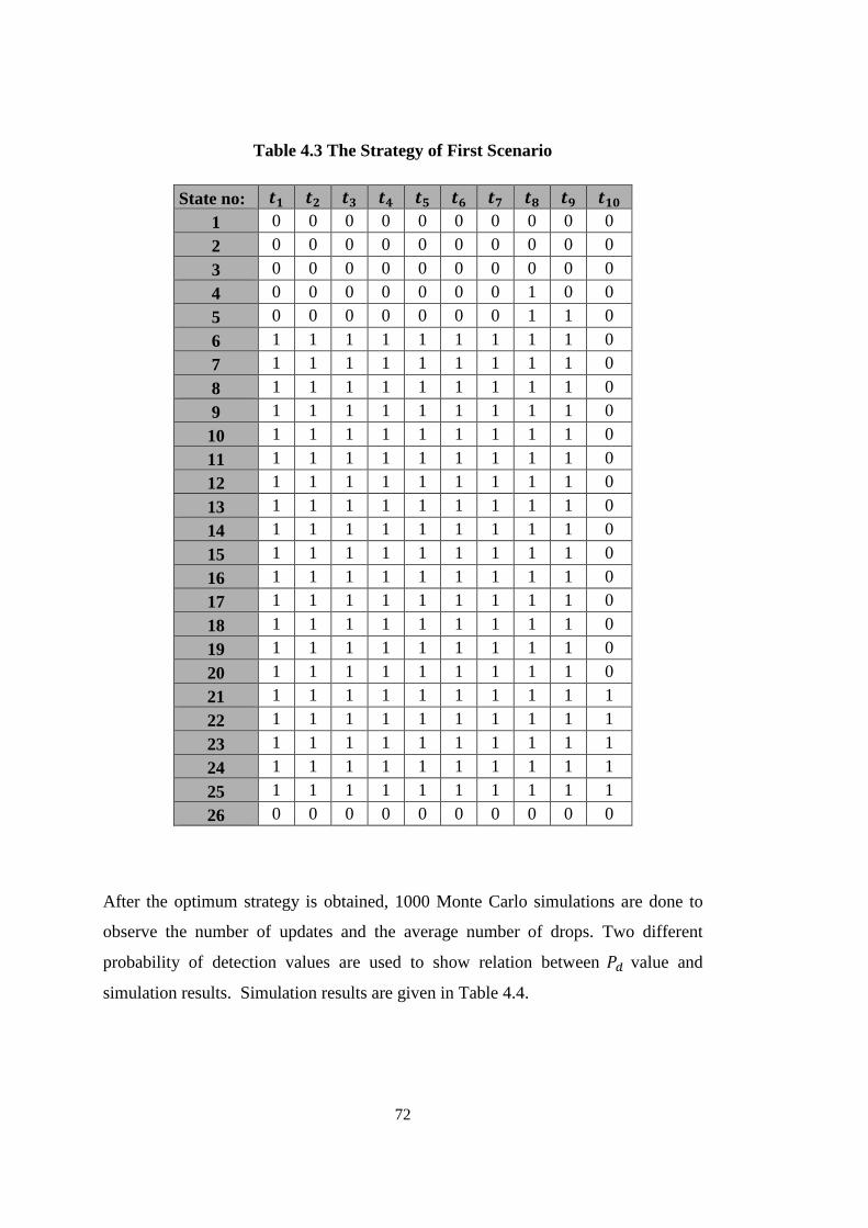
Table 4.3 The Strategy of First Scenario .................................................................... 72

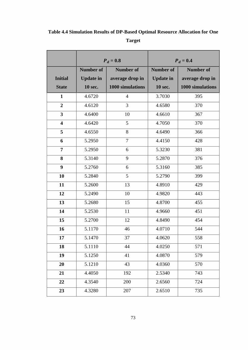
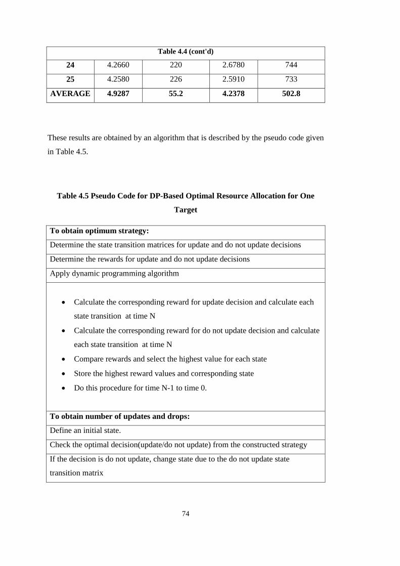
Table 4.4 Simulation Results of DP-Based Optimal Resource Allocation for One

Target .......................................................................................................................... 73

Table 4.5 Pseudo Code for DP-Based Optimal Resource Allocation for One Target 74

Table 4.6 Simulation Results of Modified DP-Based Optimal Resource Allocation

for One Target with a Rule ......................................................................................... 76

Table 4.7 Joint State Space Representation for Two Targets with Four Individual

State Markov Model ................................................................................................... 81

Table 4.8 An Example of Optimized Policy for Joint Markov Model ....................... 82

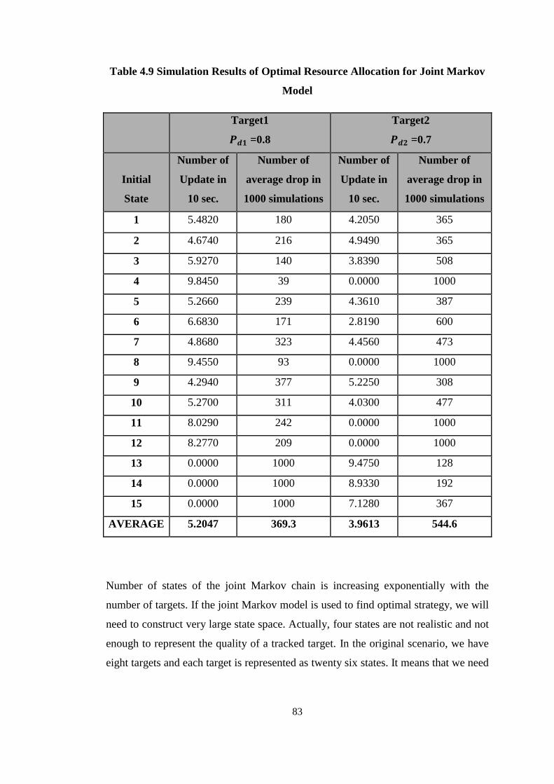
Table 4.9 Simulation Results of Optimal Resource Allocation for Joint Markov

Model .......................................................................................................................... 83

Table 4.10 An Example of Optimized Policy for Target 1 ........................................ 84

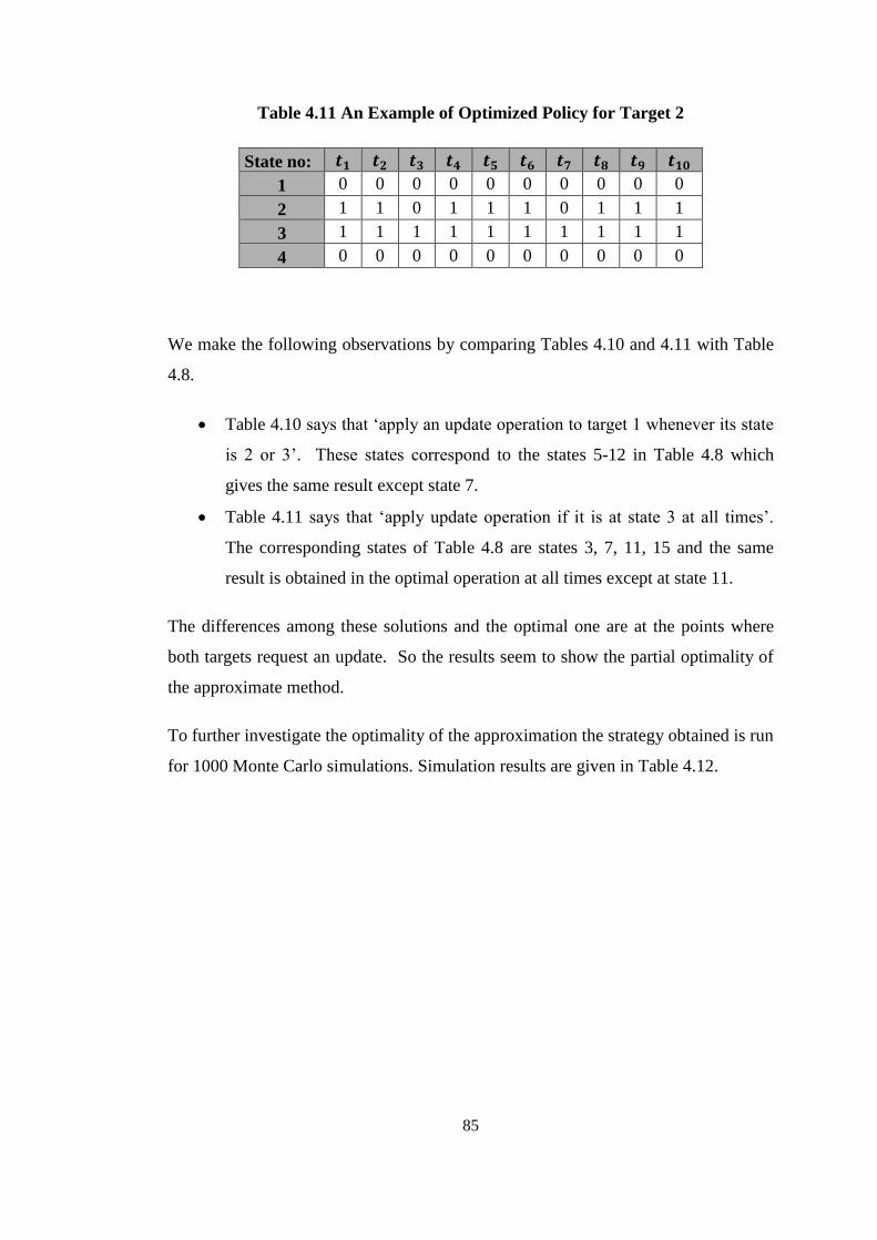
Table 4.11 An Example of Optimized Policy for Target 2 ........................................ 85

xv

Table 4.12 Simulation Results of Optimization-Based Resource Allocation with

Approximate DP ........................................................................................................ 86

Table 4.13 The Optimal Strategy of First Target ....................................................... 89

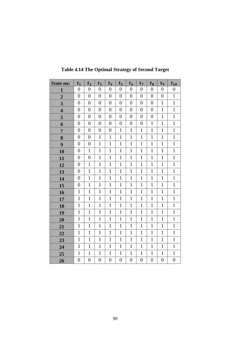
Table 4.14 The Optimal Strategy of Second Target .................................................. 90

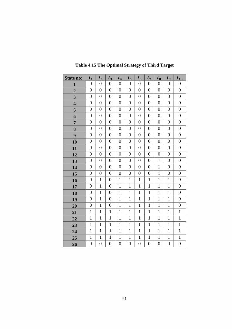
Table 4.15 The Optimal Strategy of Third Target ..................................................... 91

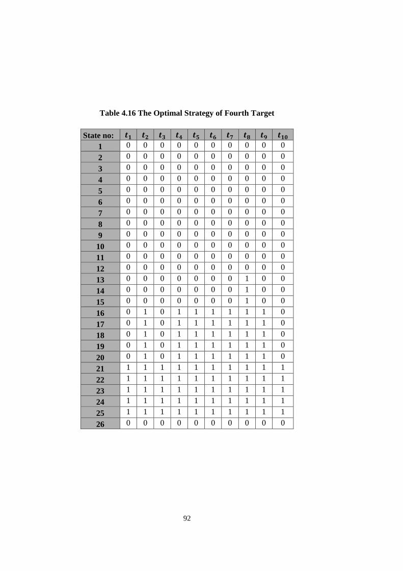
Table 4.16 The Optimal Strategy of Fourth Target ................................................... 92

Table 4.17 The Optimal Strategy of Fifth Target ...................................................... 93

Table 4.18 The Optimal Strategy of Sixth Target ...................................................... 94

Table 4.19 The Optimal Strategy of Seventh Target ................................................. 95

Table 4.20 The Optimal Strategy of Eighth Target ................................................... 96

Table 4.21 Optimal Lagrange Multipliers for Each Time Instances.......................... 97

Table 4.22 Selected Initial States of Targets.............................................................. 98


Approximate DP ........................................................................................................ 99


Approximate DP and Internal Procedure ................................................................. 101

xvi

LIST OF FIGURES

FIGURES

Figure 2.1 Block Diagram of a Pulse Radar ................................................................. 6

Figure 2.2 A Typical Radar Timeline .......................................................................... 7

Figure 2.3 Conical Scanning ........................................................................................ 8

Figure 2.4 Monopulse Scanning ................................................................................... 9

Figure 2.5 Electronically Scanning ............................................................................ 10

Figure 2.6 An Example of a Track ............................................................................. 12

Figure 2.7 The Recursive Progress of Kalman Filter ................................................. 19

Figure 2.8 An Example of an Adaptive Update Strategy ........................................... 20

Figure 2.9 Operator as Feedback Controller .............................................................. 28

Figure 2.10 Sensor Manager as Feedback Controller ................................................ 29

Figure 2.11 Partitioning Sensor Management into Macro/Micro Elements .............. 32

Figure 2.12 An Example of Macro and Micro Manager Outputs .............................. 33

Figure 2.13 An Example of a Rule Based System Taken From [30] ......................... 35

Figure 3.1 Target Motions and Priorities ................................................................... 43

Figure 3.2 A Simple Example of a 10-State Topology .............................................. 47

Figure 3.3 Target-Wise Markov Chain for Update Decision ..................................... 52

Figure 3.4 Target-Wise Markov Chain for Do Not Update Decision ........................ 53

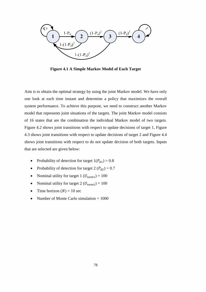
Figure 4.1 A Simple Markov Model of Each Target ................................................. 78

Figure 4.2 Joint Markov Model with Respect to Update Decisions of Target 1 ........ 79

Figure 4.3 Joint Markov Model with Respect to Update Decisions of Target 2 ........ 79

xvii

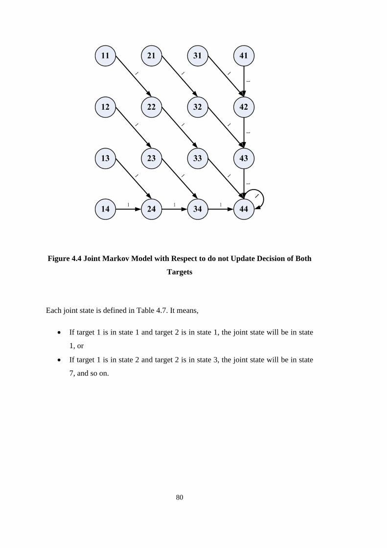
Figure 4.4 Joint Markov Model with Respect to do not Update Decision of Both

Targets ........................................................................................................................ 80

1

CHAPTER 1

1 INTRODUCTION

Radar is an acronym of “Radio Detection and Ranging” and it is an object detection

system that uses radio waves or microwaves to determine the range, direction,

altitude or speed of both moving and stationary objects. It was first developed as an

object detection system to warn of coming hostile aircraft. In recent years, radar is

the most common sensor used in tracking applications. It gives highly accurate

information about the range and the velocity of a target [1].

Perhaps the most important improvement in radar technology is the introduction of

multifunction radar in recent years. Multifunction radar systems can perform a

variety of applications that differ from old generation radar systems that perform an

individual function. By the development in solid-state technology, multifunction

radar that performs several applications within the same radar system is developed

[2].

Active electronically steered antenna radar is a type of multifunction radar whose

transmitter and receiver functions are composed of a great number of small solid-

state transmit/receive modules (TRMs). Mechanical steering is a big problem for

some radar applications especially in target tracking. To improve radar abilities an

agile beam should be constructed. Electronically steering antenna produces agile

beams without any mechanical constraint. This type of radar uses a group of

2

antennas that radiates effective pattern in a desired direction and suppresses in

undesired directions. Array of antennas are employed by using a shift in the signal

phase in order to separate desired/undesired directions. Some explanation about ESA

radars and their advantages are described in Section 2.1.3.

Electronically scanned antenna (ESA) radars have the advantage of using an agile

beam. Optimal or near optimal use of this flexibility is a challenge so there is an

increasing motivation in designing optimal radar resource allocation algorithms that

take advantage of agile beam used by ESA radars.

Sensor management deals with how to manage, coordinate and organize the usage of

scarce sensor resources in a manner of improving and optimizing the quality of

services. If there are insufficient radar resources to perform all desired tasks, the

sensor manager allocates the available resources optimally according to the some

properties such as task priority and/or maximum reward. In order to handle global

optimization problem which is highly complex to solve, usually the overall problem

is divided into many smaller sub-problems that can be considered separately.

Resource allocation is essentially a decision-making process about what information

needs to be collected from the environment and what actions need to be taken to

obtain the most desirable outcome. For target tracking, ‘update track i’ or ‘search

sector j ’ decisions are necessary to operate any tracking system. The resource

allocation can be modeled as an optimization problem for which the objective is a

function of sensor capability, number of tracked targets and also priorities of the

targets. Uncertainty management is also an important issue in tracking: The

uncertainty of the target increases when a sensor does not update a track. Therefore,

the track must be updated adaptively at acceptable time intervals to avoid track

drops. A utility function is defined to compare the benefits obtained from the

different actions. As a result of this comparison the best solution is aimed to be

chosen.

Sensor scheduling is to construct a policy which is optimal for a given objective

function under the resource constraints. More detailed information about sensor

management can be found in Section 2.4, see also [3] and [4].

3

In this thesis we present the concept of radar beam scheduling. Beam scheduling

itself is again a very complex problem. In the literature the problem is usually treated

as a two stage problem: micro level scheduling and macro level scheduling [27],

[32]. The two levels are called as slow time scale and large time scale. Slow time

scale is usually taken on the order of few seconds and with usually fixed intervals of

one second. Fast time scale aims to schedule for each interval of slow time scale so

its time intervals are in the order of milliseconds. The purposes of the two time scale

schedulers so the methods that they use are different from each other. Usually slow

time scale scheduler, called the macro scheduler, lists the jobs that should be done in

the next (slow time scale) interval and fast time scheduler, called the micro

scheduler, determines the exact times that the jobs should be done. This study aims

macro scheduling.

In this thesis the resource allocation problem is modeled as a constrained Markov

decision process. Macro management algorithm developed for multi target tracking

is based on stochastic dynamic programming. The method is very similar to the

method given in [32], which is based on constrained stochastic dynamic

programming.

The outline of the thesis is as follows:

The background information, radar theory, motion model, target tracking, Kalman

filtering, Markov chains, dynamic programming and sensor management are

introduced in Chapter 2.

In Chapter 3, the scheduling problem is stated. Its implementation is presented. The

model and algorithms that we used in this thesis are detailed.

Chapter 4 concentrates on several scenarios for stochastic dynamic programming

based resource allocation applications. Simulations are performed by proposed

algorithms and the corresponding results are compared to each other.

In Chapter 5, this thesis is concluded and some future works are suggested.

4

5

CHAPTER 2

2 THEORETICAL BACKGROUND

In this section we give brief information about the radar, target tracking and

controlled Markov chains.

2.1 Introduction to Radar Theory

Radars work on the ground, on the sea, in the air and in space. Modern radar systems

are used for early detection of surface or air objects and provide extremely accurate

information on distance, direction, height, and speed of the objects. Ground-based

radars are used to detect, locate and track the aircrafts and space targets. Shipboard

radars are used to navigate and locate buoys, shore lines and other ships, prevent

collisions on the sea, find direction at the same time observe the aircrafts. Airborne

radars are used to detect other aircrafts, ships and grounded objects. Meteorologists

use radar for monitoring weather or forecasting weather conditions. Radars are also

used in space to guide the space crafts. As you see, the modern uses of radars are

different in several areas [5]. Some detailed applications are given below.

Radars are the basic sensors in military applications. Radar types according to their

functions can be classified as: Search radars, ballistic missile defense radars, radar

seekers and fire control radars, missile support radars etc. For the civil applications,

6

they are used as process control radars, airport surveillance radars, weather radars,

marine navigation radars, satellite mapping radars, police speed measuring radars,

automotive collision avoidance radars etc.

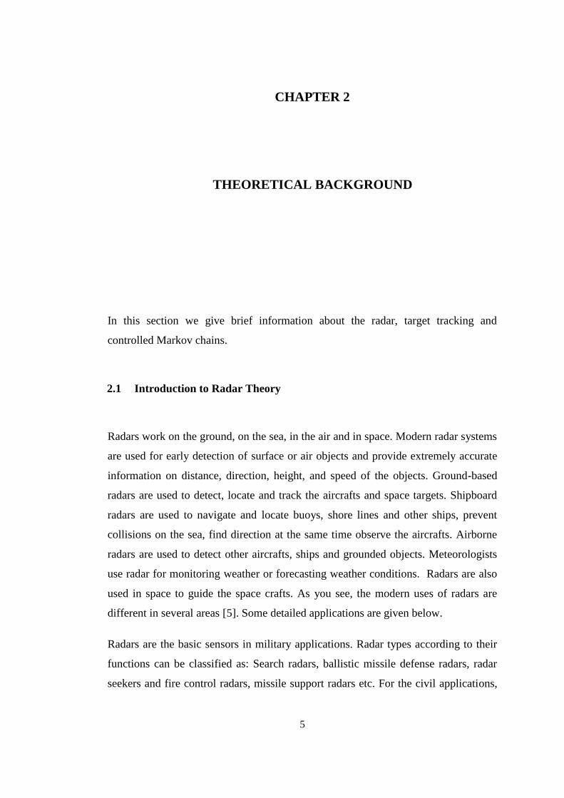
2.1.1 Fundamentals of Radar

Radar consists of a transmitter, duplexer and receiver in a very simple case. Only one

antenna is usually enough for both transmitting and receiving. The radar signal is

generated by a powerful transmitter and received by a highly sensitive receiver.

Therefore the receiver must be protected from the high power of the transmitter.

Duplexer is used for this objective. Transmitters emit radio waves called radar

signals in a particular type of waveform such as pulse modulated sine wave to the

predetermined directions. When these signals come into contact with an object they

are usually reflected in many directions. The radar signals that are reflected back

towards the transmitter are the desirable signals that make radar works. Radar

receivers are usually in the same location as the transmitter. The reflected radar

signals captured by the receiving antenna are usually very weak depending on their

travelling path and are strengthened by amplifiers [1]. A block diagram that shows

the operation of typical pulse radar is given in the Figure 2.1.

Figure 2.1 Block Diagram of a Pulse Radar

7

The most common radar waveform is a train of pulses modulating a sine wave carrier

[1]. A typical radar time line is shown in the Figure 2.2. Radar transmits a powerful

signal and waits for weak attenuated echo signal. By the time between these

operations radar can calculate the range of the target by using;

𝑅 =

𝑐 × 𝑇𝑟

2 (2.1)

where c is the speed of light, 𝑇𝑟 is the time between transmitted radar signal and

observed echo signal.

Figure 2.2 A Typical Radar Timeline

2.1.2 Types of Radar Based on Scan Pattern

Radars can be classified by the type of their scan patterns. Scanning can be defined

as the motion of the beam in a specific pattern while tracking a target or searching a

sector. In some cases, there are different scan patterns to achieve some particular

system functions such as searching or tracking.

8

Conical Scan: Conical scanning is the simplest type of scanning. In this type, a radar

beam is produced by the mechanically steered antenna. Antenna rotates 360° to cover

the azimuth plane and beam is produced in the direction of antenna’s main lobe. If

there is a target on the bore sight line, maximum reflection will occur. When the

target is away from the main lobe of the beam, reflected radar signal will decrease

due to the distance from the bore sight. Target location can be found by the received

maximum reflected signal. The disadvantages of conical scan type radars are the

mechanical constraints and large side lobes which lead to signal losses and reduce

the sensitivity of the variation in the received signal. It means that the target position

is determined only by the power of the received signal and variations will cause

misleading results. A typical conical scanning is shown in the Figure 2.3.

Figure 2.3 Conical Scanning

Track-While-Scan (TWS) Radars: TWS Radars allocate part of its resources to

tracking targets while remaining part of its resource is used for searching for new

targets. The disadvantage of TWS radars is to be highly vulnerable to jamming

because of wide area scanning.

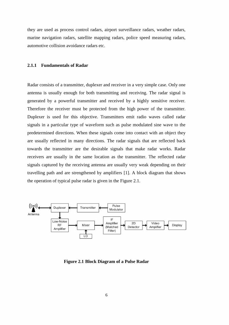
Monopulse Scan Radars: This type of radar is similar to conical scan type radars.

The difference is to split the beam into sectors that are called lobes and send radar

9

signals in slightly different directions. Received signals are compared to each other.

A typical monopulse scanning is shown in the Figure 2.4.

Figure 2.4 Monopulse Scanning

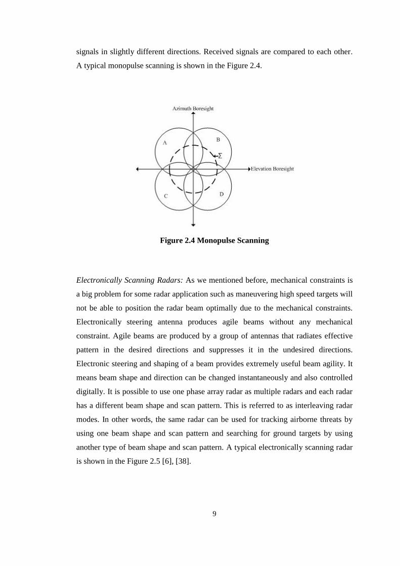
Electronically Scanning Radars: As we mentioned before, mechanical constraints is

a big problem for some radar application such as maneuvering high speed targets will

not be able to position the radar beam optimally due to the mechanical constraints.

Electronically steering antenna produces agile beams without any mechanical

constraint. Agile beams are produced by a group of antennas that radiates effective

pattern in the desired directions and suppresses it in the undesired directions.

Electronic steering and shaping of a beam provides extremely useful beam agility. It

means beam shape and direction can be changed instantaneously and also controlled

digitally. It is possible to use one phase array radar as multiple radars and each radar

has a different beam shape and scan pattern. This is referred to as interleaving radar

modes. In other words, the same radar can be used for tracking airborne threats by

using one beam shape and scan pattern and searching for ground targets by using

another type of beam shape and scan pattern. A typical electronically scanning radar

is shown in the Figure 2.5 [6], [38].

10

Figure 2.5 Electronically Scanning

2.1.3 Electronically Steered Antenna Radars

Electronically steered antenna (ESA) radars have the advantage of having an agile

beam that means transmitted energy can be allocated adaptively in space and time.

Radars that are equipped with an electronically steered antenna have the capability of

directing the radar beam without mechanically adjusting the antenna. Furthermore,

the beam can be redirected instantaneously towards any location in space. Hence, the

mechanical constraint of a traditional antenna is relaxed. It is a significant

improvement that targets can be observed in any order in multiple target tracking

applications.

ESA radar has several advantages compared to ordinary radar systems.

The direction of the radar beam is not fixed to the antenna,

ESA radars have the ability to adaptively allocate radar energy in time and

space where the demand is highest.

SAR

&

GMTI

MISSILE GUIDANCE

SUPPORT

SEARCHING

TRACKING

11

ESA radars have the ability to send beams in different directions and in an

arbitrary order, so the high priority targets can be observed more frequently.

ESA radars permit spending more time on one particular measurement. On

the other hand, less time will then be available for other tasks.

The earliest phased array antenna system called as passive electronically scanned

array (PESA) has one large central power amplifier tube to send the energy into

phase shift modules for adjusting signal phases in a desired direction by using

various emitting elements in the front of the antenna. On the other hand, an active

electronically scanned array (AESA) device, also known as active phased array radar

(APAR), has individual source in each emitting elements. Transmitter and receiver

functions are merged in small solid-state transmit/receive modules (TRMs).

Therefore, PESA radar is simpler and cheaper to construct than an AESA. But, the

AESA architecture has significant advantages such as controlling the amplitude and

phase of each element, adaptively.

Thus, the allocation of time and energy to various tasks is important for the overall

performance of the radar system. The problem of resource allocation can be defined

as “how to adaptively allocate the constrained radar resource in time and space to

handle all tasks in the optimal way”. This can be solved by designing a measurement

policy that optimally utilizes the radar resources. Sensor management is used to

achieve this purpose. The concepts of sensor management and radar resource

management will be explained in Section 2.4.

2.2 Target Tracking

The aim of this thesis is to track multiple targets by ESA radar efficiently. In this

section we will give brief information about the tracking problem and briefly define

what tracking is and one of the motion models that is mostly used: constant velocity

model.

12

A target is anything whose state interests us. On the other hand, a track is a state

trajectory estimated from a sequence of measurements that has been associated with

a single source. Measurements are noisy observations related to the (partial) state of

a target. Generally each arriving measurement starts or updates a track. Tracking is

the processing of measurements obtained from a target in order to maintain an

estimate of target’s current state [7]. Detection is to know the presence of an object,

meanwhile tracking is to maintain a state of an object over time. It maintains the

object‘s state and identity despite detection errors (false negatives, false alarms),

occlusions, and in the presence of other objects. An example that explains the

tracking process is given below in Figure 2.6 [8].

Figure 2.6 An Example of a Track

According to their different life stages, tracks can be classified into three cases [9].

13

Tentative (initiator): A track that is in the track initiation process. We are not sure

that there is sufficient evidence that it is actually a target or not.

Confirmed: A track that is decided to belong to a valid target.

Deleted: A track that is decided to come from false alarms.

Tracker uses the measurements obtained from the neighborhood of the predicted

position of a target to maintain the track. The predicted position is delivered by the

motion model. Several problems are involved in this procedure. One problem is the

computation of the predicted position. This is done by using the motion model of the

target. However since motion of a target is not static usual practice is to use several

models. Another problem is how to use the new measurement for track maintenance.

For simple linear motion models Kalman filter seems to be the best tool for this

purpose. For more complicated realistic cases some algorithms derived from the

Kalman filter are used. Measurement-track association is another important issue.

There are several ways of solving the association problem starting from the rule

‘associate the nearest measurement’ towards very complicated algorithms like

‘multiple hypothesis tracking’.

In the remaining part of this sub section we will explain the simplest model that can

be used for tracking so called constant velocity model. Then we explain the Kalman

filter very briefly.

2.2.1 Motion Model: The Constant Velocity Model

The motion model is a state space model of the track motion, usually linear and the

measurements are the position of the target in the 3D or 2D space. Kalman filtering

and its variations are the mostly used tools in tracking problems.

The simplest model that is used for a tracking system is the ‘constant velocity’

model. It is used to represent the non-maneuvering targets motion. As its name

14

implies model assumes that the target is moving on a straight line with constant

velocity. Here we explain the constant velocity model.

Let 𝑝(𝑡) denote the target position, so the velocity is the first order derivative of the

position, 𝑣(𝑡) = �̇�(𝑡) and the acceleration is the second order derivative of the

position 𝑎(𝑡) = �̈�(𝑡) . Since we will use constant velocity model, acceleration is

assumed to be almost zero so is modeled as a zero mean white Gaussian noise.

�̈�(𝑡) = 𝑤(𝑡) (2.2)

The state equations in one dimension are:

𝑥 = [ 𝑝 𝑝 ̇ ] ; �̇�(𝑡) = [

0 10 0

] 𝑥(𝑡) + [ 0 1

] 𝑤(𝑡) (2.3)

The model is usually used in discrete time since the measurements are obtained at

discrete times. The discrete time equivalent of the above continuous time model is as

follows.

Let 𝑝𝑘 𝑎𝑛𝑑 𝑣𝑘 denote the target position and velocity at time 𝑡𝑘.

𝑥𝑘 = [ 𝑝𝑘 𝑣𝑘

] and 𝑇 = 𝑡𝑘+1 − 𝑡𝑘 (2.4)

For real world, the perfect constant velocity assumption is unrealistic. Therefore

some variation of velocity that is described by piecewise constant white acceleration

is applied. The relaxed state equations then become:

15

𝑝𝑘+1 = 𝑝𝑘 + 𝑣𝑘𝑇 +

1

2𝑤𝑘𝑇

2 (2.5)

𝑣𝑘+1 = 𝑣𝑘 + 𝑤𝑘𝑇 (2.6)

where 𝑤𝑘 is called as process noise and it is a zero-mean Gaussian white noise:

𝑤𝑘~𝑁(0, 𝜎𝑤2(𝑘))

𝑥𝑘+1 = [

𝑝𝑘+1 𝑣𝑘+1

] = [1 𝑇0 1

] . 𝑥𝑘 + [ 1

2𝑇2

𝑇

] . 𝑤𝑘

[ 1

2𝑇2

𝑇

] . 𝑤𝑘~𝑁(0, 𝑄(𝑘))

(2.7)

For n-Dimensional Cartesian coordinate system, state equations are similarly;

𝑥𝑘+1 = [𝐼𝑛𝑥𝑛 𝑇. 𝐼𝑛𝑥𝑛

0𝑛𝑥𝑛 𝐼𝑛𝑥𝑛] . 𝑥𝑘 + [

1

2. 𝑇2 . 𝐼𝑛𝑥𝑛

𝑇 . 𝐼𝑛𝑥𝑛

] . 𝑤𝑘

[ 1

2. 𝑇2 . 𝐼𝑛𝑥𝑛

𝑇 . 𝐼𝑛𝑥𝑛

] . 𝑤𝑘~𝑁(0, 𝑄(𝑘))

(2.8)

where 𝑄(𝑘) = [

1

4𝑇4𝐼𝑛𝑥𝑛

1

2𝑇3𝐼𝑛𝑥𝑛

1

2𝑇3𝐼𝑛𝑥𝑛 𝑇2𝐼𝑛𝑥𝑛

] 𝜎𝑤2(𝑘) characterize the modeling uncertainty

and 𝜎𝑤2(𝑘) should be related to the acceleration magnitude.

16

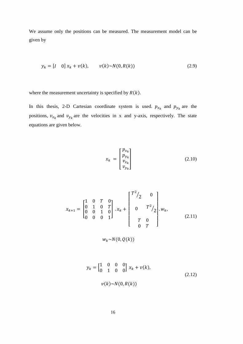
We assume only the positions can be measured. The measurement model can be

given by

𝑦𝑘 = [𝐼 0] 𝑥𝑘 + 𝑣(𝑘), 𝑣(𝑘)~𝑁(0, 𝑅(𝑘)) (2.9)

where the measurement uncertainty is specified by 𝑅(𝑘).

In this thesis, 2-D Cartesian coordinate system is used. 𝑝𝑥𝑘 and 𝑝𝑦𝑘

are the

positions, 𝑣𝑥𝑘and 𝑣𝑦𝑘

are the velocities in x and y-axis, respectively. The state

equations are given below.

𝑥𝑘 = [

𝑝𝑥𝑘

𝑝𝑦𝑘

𝑣𝑥𝑘

𝑣𝑦𝑘

] (2.10)

𝑥𝑘+1 = [

1 00 1

𝑇 00 𝑇

0 00 0

1 00 1

] . 𝑥𝑘 +

[

𝑇2

2⁄ 0

0 𝑇2

2⁄

𝑇 00 𝑇 ]

. 𝑤𝑘,

𝑤𝑘~𝑁(0, 𝑄(𝑘))

(2.11)

𝑦𝑘 = [1 0 0 00 1 0 0

] 𝑥𝑘 + 𝑣(𝑘),

𝑣(𝑘)~𝑁(0, 𝑅(𝑘))

(2.12)

17

where 𝑄(𝑘) and 𝑅(𝑘) characterize the modeling uncertainty and measurement

uncertainty. An accurate estimate of the state 𝑥𝑘 is needed to control the system. This

is achieved by the Kalman filter.

The constant velocity model is too simplistic for many applications. This is mainly

due to the unknown nature of the motion of the target: targets usually maneuver in

some time intervals that the constant velocity model is insufficient. To overcome the

motion uncertainties, more than one model is used in most applications [7], [10].

Interactive Multiple Model (IMM) is a famous modeling technique used for this

purpose [7].

2.2.2 The Kalman Filter

Target tracking is a state estimation problem. A state space model is constructed in

the previous section. 2-D motion state includes the target position and velocity in

each axis at every time instant and observation model models the relationship with

the current target state and the current observations. Over the past half century many

techniques have been developed for target tracking. All of the techniques are related

with the classical Kalman filtering, so here we explain the Kalman filter briefly. If

the state model is linear and process and measurement noise are modeled as zero-

mean Gaussian white, the Kalman filter is the optimal estimator in the minimum

mean square error (MMSE) sense [11].

The Kalman filter is a recursive data processing algorithm that generates optimal

estimate of the states given the set of measurements. For the linear Gaussian system

the posterior density at every time step becomes Gaussian and so is characterized by

its mean and covariance matrix. The state space equations that are used in Kalman

filtering are as follows.

18

𝑥𝑘 = 𝐴 . 𝑥𝑘−1 + 𝑤𝑘−1, 𝑤𝑘−1~𝑁(0, 𝑄) (2.13)

𝑦𝑘 = 𝐻 𝑥𝑘 + 𝑣𝑘, 𝑣𝑘~𝑁(0, 𝑅) (2.14)

where 𝐴 and 𝐻 are known system and measurement matrices that define the linear

function. Random variables 𝑤𝑘 and 𝑣𝑘 are mutually independent zero-mean white

Gaussian with covariances 𝑄𝑘 and 𝑅𝑘 respectively.

Kalman filtering can be divided into two parts as prediction and correction [12].

Prediction Step:

�̂�𝑘|𝑘−1 = 𝐴 �̂�𝑘−1|𝑘−1 (2.15)

𝑃𝑘|𝑘−1 = 𝐴 𝑃𝑘−1|𝑘−1𝐴𝑇 + 𝑄𝑘−1 (2.16)

Correction Step:

�̂�𝑘|𝑘 = �̂�𝑘|𝑘−1 + 𝐾𝑘 (𝑦𝑘 − 𝐻 �̂�𝑘|𝑘−1) (2.17)

𝑃𝑘|𝑘 = 𝑃𝑘|𝑘−1 − 𝐾𝑘 𝑆𝑘 𝐾𝑘𝑇 (2.18)

where

�̂�: Estimated state

𝐴: State transition matrix

𝑃: State variance matrix

𝑄: Process variance matrix

𝑅: Measurement variance matrix

19

𝑦𝑘: Measurement

𝐻: Measurement matrix

𝑆𝑘 = 𝐻𝑘𝑃𝑘|𝑘−1𝐻𝑘𝑇 + 𝑅𝑘 is the covariance of the innovation term (𝑦𝑘 − 𝐻 �̂�𝑘|𝑘−1)

𝐾𝑘 = 𝑃𝑘|𝑘−1𝐻𝑘𝑇𝑆𝑘

−1 is the Kalman gain. Note that, covariance update can be

rewritten as;

𝑃𝑘|𝑘 = (𝐼 − 𝐾𝑘𝐻𝑘) 𝑃𝑘|𝑘−1 (2.19)

where 𝐼 is the identity matrix of dimension 𝑛𝑥𝑛.

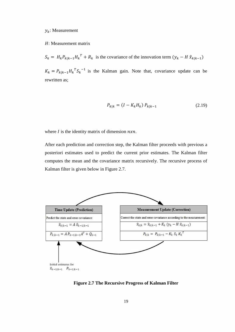
After each prediction and correction step, the Kalman filter proceeds with previous a

posteriori estimates used to predict the current prior estimates. The Kalman filter

computes the mean and the covariance matrix recursively. The recursive process of

Kalman filter is given below in Figure 2.7.

Figure 2.7 The Recursive Progress of Kalman Filter

20

2.2.3 Adaptive Target Tracking

Track update rates need not be the same for all targets. An extreme example is that a

ship and a missile clearly shouldn’t be updated at the same rate due to the slow

motion of the first one compared to the agility of the second. The update rate

depends on the uncertainty of the state of the target compared to the beam width. If

target uncertainty is low enough, radar resource can be used for other targets. By this

way, more targets can be tracked in an acceptable uncertainty level. In Kalman

filtering uncertainty parameter of the target (state covariance matrix) reaches the

steady state value exponentially in case of regular updates. Therefore, after a few

updates, uncertainty reaches its steady state value. However if the target is not

updated, the error covariance matrix will continue to increase exponentially. When

this value is under a certain threshold value, track does not need to be updated. An

illustration is shown in Figure 2.8 below.

Figure 2.8 An Example of an Adaptive Update Strategy

21

Adaptive update strategy is useful when limited radar resource is not enough to track

desired number of targets. To find a reasonable update strategy for each target is the

tracking scheduling problem. In Section 4.1 and Section 4.2, an optimal update

strategy is constructed by using dynamic programming for one sensor and one target.

2.3 Markov Chains

The model used for solving the scheduling problem is a controlled Markov chain. So

in this section we briefly explain what a Markov chain and a Markov Decision

Process (MDP) are.

Markov process is a stochastic process that the conditional distribution at any time

given the value at the previous times is same as the case that only the last value is

given. For the discrete time and finite state case Markov process is named as ‘finite

state Markov chain’. When we have a control on the system, usually Markov chain is

named as controlled Markov chain. In some systems it may not be possible to exactly

know the state of the chain but only an observation is given related statistically with

the state. The name used for the two cases is either Hidden Markov Model (HMM) if

chain is not controlled or Partially Observable Markov Decision Process (POMDP) if

control exists. The summary of this classification is given in Table 2.1.

Table 2.1 The Markov Models

System state is fully

observable

System state is partially

observable

System is autonomous Markov Chain Hidden Markov Model

System is controlled Markov Decision Process Partially Observable

Markov Decision Process

The formal definition of a Markov chain and some of its properties are given below.

22

2.3.1 Markov Property

This subsection gives a more formal approach to Markov chains.

Let Ω = {𝑎1 , 𝑎2 … 𝑎𝑁} be the set of states 𝑥𝑡 of a system. A Markov chain is a

triple (Ω, P, 𝑃0) where Ω is the finite set of states, P is the transition probability

matrix and 𝑃0 = 𝑃𝑟(𝑥0) is the initial probability vector. This triple satisfies the

following axioms:

1) The probability 𝑃𝑟 for each state of the system satisfies the Markov property

i.e.,

𝑃𝑟( 𝑥𝑡|𝑥0, 𝑥1, 𝑥2, 𝑥3, … 𝑥𝑡−1) = 𝑃𝑟(𝑥𝑡|𝑥𝑡−1) (2.20)

2) A transition matrix of a Markov chain is called stochastic matrix which is a

square matrix that has non-negative elements and each row sum is equal to 1.

For a system that has the N × N state transition matrix is defined by:

𝑃 = (𝑝𝑖𝑗) 1 ≤ 𝑖, 𝑗 ≤ 𝑁 (2.21)

where 𝑝𝑖𝑗 = 𝑃𝑟(𝑥𝑡+1 = 𝑎𝑗|𝑥𝑡 = 𝑎𝑖) ≥ 0 and ∑ 𝑝𝑖𝑗𝑁𝑗=1 = 1 𝑓𝑜𝑟 𝑖 = 1, 2…𝑁

3) 𝑃0 = 𝑃𝑟(𝑥0) is the initial probability vector.

23

Let us consider n-step transition probabilities pijn in terms of P. The probability,

starting in state i, of going to state j in two steps is the sum over k of the probability

of going first to k and then to j. Using the Markov property in (2.20):

𝑝𝑖𝑗2 = ∑ 𝑝𝑖𝑘

𝑁

𝑘=1

𝑝𝑘𝑗 (2.22)

It can be seen that this is just the 𝑖𝑗 term of the product of the matrix 𝑃 with itself,

i.e., that pij2 is the 𝑖, 𝑗 element of the matrix 𝑃2. Similarly,

pijn is the 𝑖𝑗 element of the nth power of the matrix 𝑃. Since 𝑃𝑚+𝑛 = 𝑃𝑚 𝑃𝑛

pijm+n = ∑ 𝑝𝑖𝑘

𝑚

𝑁

𝑘=1

𝑝𝑘𝑗𝑛 (2.23)

This is known as the Chapman–Kolmogorov equation.

Let 𝑃𝑡 denote the vector of the probabilities of each state at time 𝑡:

𝑃𝑡 = 𝑃𝑟(𝑥𝑡) = (

𝑃𝑟(𝑥𝑡 = 𝑎1)

𝑃𝑟(𝑥𝑡 = 𝑎2)⋮

𝑃𝑟(𝑥𝑡 = 𝑎𝑁)

)

𝑇

(2.24)

Note that 𝑃𝑡 satisfies following relation:

𝑃𝑡 = 𝑃𝑡−1𝑃 = 𝑃0𝑃𝑡 (2.25)

24

2.3.2 Regular (Ergodic) Markov Chain

N-state Markov chain is regular (ergodic) if 𝑃𝑖𝑗(𝑘) > 0 for all 𝑖, 𝑗, and all 𝑘 ≥ (𝑁 −

1)2 + 1 [13]. This means that it is possible to go from any state 𝑆𝑖 to any state 𝑆𝑗 in 𝑘

steps with nonzero probability. A property of regular Markov chains is that the

powers of 𝑃 converge, or lim𝑛→∞(𝑃)𝑛 = Π where the rows of Π are identical. It is

known that for the regular Markov chains one eigenvalue of 𝑃 is equal to 1 and all

others are less than 1 in magnitude. Let 𝜔 = [𝜔1 𝜔2 … 𝜔𝑛] be the unique normalized

left eigenvector of 𝑃 corresponding to the eigenvalue one. For the regular chains

𝜔𝑖 > 0 for all 𝑖 and ∑ 𝜔𝑖𝑁𝑖=1 = 1. That is 𝜔𝑃 = 𝜔 . Furthermore each row of Π is

equal to 𝜔 and 𝑃𝑛 → 𝑃0Π = 𝜔. That means at the steady state the probability of

being in state 𝑆𝑖 is 𝜔𝑖, 1 ≤ 𝑖 ≤ 𝑁 independent of the initial condition 𝑃0.

2.3.3 Absorbing Markov Chain

A state 𝑆𝑖 is absorbing if 𝑝𝑖𝑖 = 1, so 𝑝𝑖𝑗 = 0 for 𝑖 ≠ 𝑗. That means once you are in

the state 𝑆𝑖, you can never leave it. Suppose there are 𝑘 absorbing states, 1 ≤ 𝑘 ≤ 𝑁,

and then we may rename the states (if needed) so that the transition matrix 𝑃 can be

written as

𝑃 = (

𝐼 𝑂𝑅 𝑄

) (2.26)

where 𝐼 is the 𝑘 𝑥 𝑘 identity, 𝑂 is the 𝑘 𝑥 (𝑁 − 𝑘) zero matrix. 𝑅 is (𝑁 − 𝑘) 𝑥 𝑘 and

𝑄 is (𝑁 − 𝑘) 𝑥 (𝑁 − 𝑘). The Markov chain is called an absorbing Markov chain if it

has at least one absorbing state. The expected time of reaching an absorbing state

from a non-absorbing state is finite. Note that for the absorbing chains we have

25

𝑃𝑛 = (

𝐼 𝑂𝑆𝑅 𝑄𝑛) (2.27)

where 𝑆 = 𝐼 + 𝑄 + ⋯+ 𝑄𝑛−1.

Then, lim𝑛→∞(𝑃)𝑛 = Π where

Π = (𝐼 𝑂𝑅∗ 𝑂

) (2.28)

for 𝑅∗ = (𝐼 − 𝑄)−1𝑅. Notice the zero columns in Π which imply that the probability

that the process will eventually enter an absorbing state is one. The process

eventually ends up with an absorbing state.

2.3.4 Markov Chain with Rewards

In some applications like the scheduling problem, a reward 𝑅𝑖 is associated to each

state 𝑆𝑖 of the Markov chain. When Markov chain evolves, total reward is collected

and it depends on the states that are visited by the chain. So the aggregated reward is

related to the state transition matrix 𝑃. In this thesis, the reward of each state is

related with the parameterized error covariance matrix. To increase the aggregated

reward a parameter called the control variable would be necessary. Possibility of

selecting the control parameter for each time instant makes the system a Markov

Decision Process. In Section 2.3.5 and Section 2.5 we explain Markov Decision

Processes and the corresponding optimal control methodology: dynamic

programming.

26

2.3.5 Markov Decision Process

MDP explained here is based on [13]. Markov decision process (MDP) is a

mathematical model for decision making in situations where outcomes are partly

under the control of a decision maker and partly random.

A Markov decision process is a 5-tuple (Ω, U, 𝑃.(.. , .. ), 𝑅.(.. , .. ), 𝛾) where;

Ω is a finite set of states,

U is a finite set of actions, (alternatively, 𝑈𝑠 is the finite set of actions

available from state s),

𝑃𝑈( 𝑆𝑖, 𝑆𝑗) = Pr (𝑆𝑡+1 = 𝑆𝑗|𝑆𝑡 = 𝑆𝑖, 𝑈𝑡 = 𝑈) is the probability that action 𝑈

in state 𝑆𝑖 at time 𝑡 will lead to state 𝑆𝑗 at time 𝑡 + 1.

𝑅𝑈( 𝑆𝑖, 𝑆𝑗) is the immediate reward (or expected immediate reward)

received after transition to state 𝑆𝑗 from state 𝑆𝑖,

𝛾 ∈ [0, 1] is the discount factor, which represents the difference in

importance between future rewards and present rewards.

The total reward that must be maximized is the expected total reward that can be

written as

𝐸 {∑𝛾𝑡𝑅𝑈(𝑡)( 𝑆𝑖(𝑡), 𝑆𝑗(𝑡))

𝑇

𝑡=1

} (2.29)

With this objective function the optimization problem can be written as

max𝑈(𝑡)

𝐸 {∑𝛾𝑡𝑅𝑈(𝑡) ( 𝑆𝑖(𝑡), 𝑆𝑗(𝑡))

𝑇

𝑡=1

} (2.30)

27

The problem is: At each time instant 𝑘, the Markov process is in some state 𝑆𝑖 and

the decision maker may choose any action 𝑈 that is available in state 𝑆𝑖. The process

moves randomly into a new state at the next time instant 𝑘 + 1 according to the

given controlled Markov chain and this movement between states has a

corresponding reward 𝑅𝑈( 𝑆𝑖, 𝑆𝑗) . The chosen action affects the probability of

moving to a new state 𝑆𝑗 . State transition matrix that depends on the decision

action 𝑈, gives the probability of moving to a new state 𝑆𝑗. Therefore, the state 𝑆𝑗 in

next time instant 𝑘 + 1 depends on the current state and the decision action 𝑈 that

we made. On the other hand, it is conditionally independent of all previous states and

actions given that 𝑆𝑖 and 𝑈. The difference between Markov chain and MDP is the

addition of actions ( 𝑈𝑖′𝑠) and rewards (𝑅𝑈( 𝑆𝑖, 𝑆𝑗)). Conversely, if only one action

exists for each state and all rewards are the same a Markov decision process reduces

to a Markov chain.

Decision maker uses a set of rules that is called as ‘policy’ in selecting alternative at

each time. The aim of MDPs is to find a decision policy that can be represented as a

matrix that relates the states to the decisions. We want to consider the expected

aggregate reward over a long time interval such as n steps of the ‘Markov chain’ as a

function of the policy used by the decision maker. There are two types of policies

that can be used by the decision maker. If the fixed decision is made for all states

independent of time, past decisions and past transitions, it is called as stationary

policy. On the other hand, optimal policy is used to maximize the expected aggregate

reward over a long time interval. Optimal policy changes depend on the selected

length of the long time interval. A final reward should be determined appropriately.

Optimal dynamic policy for that final reward is an optimized strategy and is a

function of the length of the long time interval and the determined final reward. The

objective is to generate an optimal policy that will maximize the random aggregated

reward in a finite time horizon. This policy can be found by using the dynamic

programming algorithm which is defined in Section 2.5.

28

2.4 Resource Management

The aim of the resource management is to optimize the overall performance and

effectively perform tasks of detecting new targets and track the existing ones in a

tracking system by allocating the available resources. The main resource of the

problem mentioned here is the time. The parameters that determine the effectiveness

of the use of this resource are usually track loss, tracks that are not initiated, track

uncertainty or quality and track priority.

The state error covariance matrix gives the information about the current state quality

of the tracking system. The part of the state error covariance matrix that corresponds

to the target position is usually used in the scheduling problems. State error

covariance matrix is obtained from the filter output which is a variant of Kalman

filtering for most of the time [14], [15], [16]. For example in [16] multi sensor

scheduling method by using IMM filtering is presented.

Sensor manager tries to optimize the overall system performance usually by using

the track quality derived from the covariance matrix and the related reward function.

Figure 2.9 Operator as Feedback Controller

29

Figure 2.10 Sensor Manager as Feedback Controller

The role of automatic sensor management, compared to human operator, is to control

the future sensor behavior while the operator still makes higher order tactical

decisions. Note that in a system without sensor management, the operator makes all

decisions related to the sensor for the next measurement time. On the other hand in a

system with sensor management, primary feedback is provided by the sensor

manager, under the possible guiding input from the operator. Figure 2.9 and Figure

2.10 illustrate the situations above.

Major advantages of sensor management can be summarized as follows.

Reduced pilot workload:

Past information is used to determine the future behavior of the sensor

by the sensor management.

The operator is responsible to give only higher level decisions (tracks

priority, degree of active radiation)

30

Sensor tasking based on finer detail:

Only limited amount of detail is displayed on screen, not the all

information

Therefore, operator focuses the tactical decision more deeply.

Faster adaptation:

Since sensor management system is automated, it has faster

adaptation to changing environment.

Other necessities of the sensor management:

Effective use of limited radar resources

Track maintenance

Sensor fusion and synergism

Support of specific goals

2.4.1 Radar Resource Management

This section gives general information about radar resource management which is

more general then only scheduling. Radar resource management algorithms aim to

enhance the overall radar system performance. The resource allocation problem of

efficiently conducting several parallel tracking and searching tasks using the radar’s

antenna is an important part of the scheduling problem that needs to be considered.

Due to the stochastic nature of radar detection and target dynamics, scheduling of

radar measurements is a stochastic control problem [39].

The selection of all parameters that define the operation of the sensor determines the

allocation of the limited resources. Parameters can be general tactical decisions, field

of view, scanning types, measurement scheduling, waveform selection and

processing directives. Each of these parameters is specified by a number of degrees

of freedom. For example, waveform selection entails frequency, pulse repetition

31

frequency (PRF), length of coherent integration and total time on target. The overall

system performance depends on all these parameters. The overall system

performance can be divided into two views to be managed. The parameter view of

sensors and the mode view of sensors. The parameter view of managing sensors

requires the sensor manager to directly control each parameter and the mode view is

the upper level manager that simplifies the sensor management decision making.

This is called as two-level two-timescale scheduling. Mode and parameter view of

sensors refer as macro and micro management, respectively [17].

Two-Level Two-Timescale Scheduling

Scheduling of radar measurements naturally decomposes into two different scales.

Macro level includes all high level tasking best summarized by the expression which

task should the sensor perform. On the other hand micro level includes low level

tasking such as how a particular Macro-task can be accomplished best. A few macro

and micro manager tasks are given in Table 2.2, as examples [18], [19].

Table 2.2 Examples of Micro & Macro Level Tasks

Micro Level Tasks

(Parameter Design)

Macro Level Tasks

(Mode Selection) Pulse Reputation Frequency (PRF) Long Range Search

Pulse Width Self-Protect Search

Coherent Integration Fire Control Search

Time on Target Alert Acquisition

Detection Threshold Track Update

Peak Transmitted Power Track Confirm

Average Transmitted Power Track ID Update

Target Revisit Time ECM Assessment

Aperture Beamwidth ECCM Support

As stated before in this study we are only interested in the scheduling problem so in

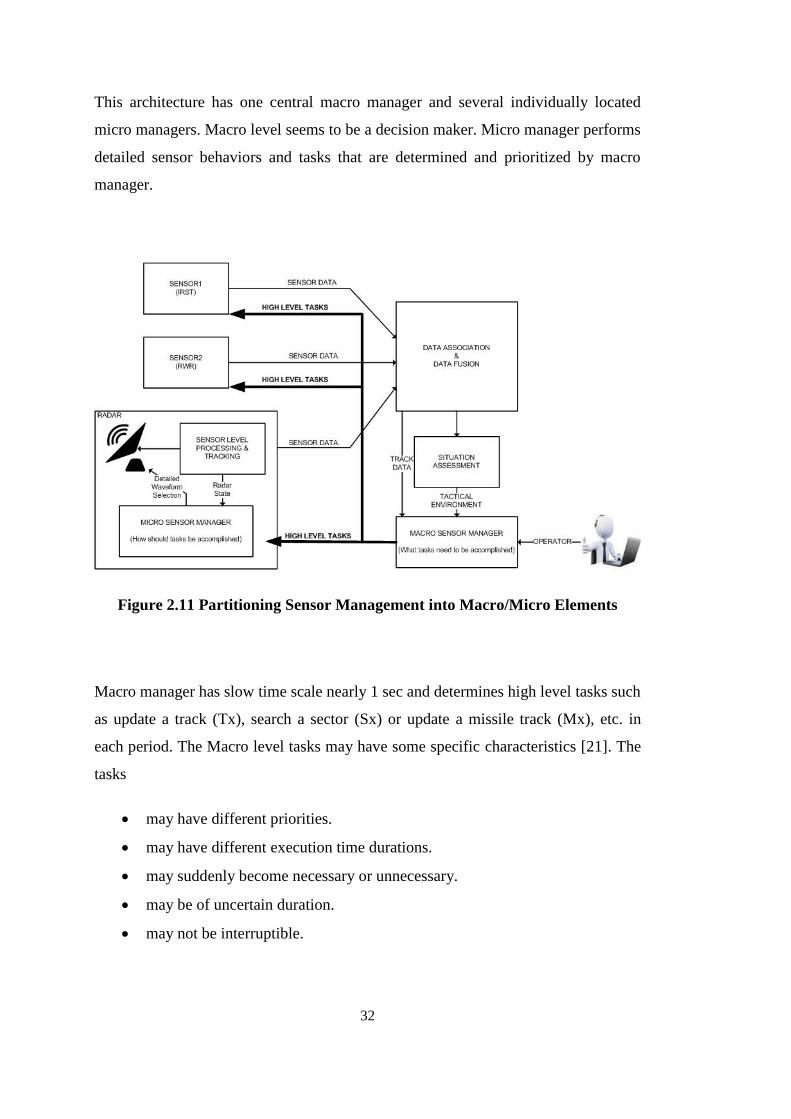
the remaining part we will concentrate on this subject. An example of sensor

management architecture for multi sensor system is shown in the Figure 2.11. [20]

32

This architecture has one central macro manager and several individually located

micro managers. Macro level seems to be a decision maker. Micro manager performs

detailed sensor behaviors and tasks that are determined and prioritized by macro

manager.

Figure 2.11 Partitioning Sensor Management into Macro/Micro Elements

Macro manager has slow time scale nearly 1 sec and determines high level tasks such

as update a track (Tx), search a sector (Sx) or update a missile track (Mx), etc. in

each period. The Macro level tasks may have some specific characteristics [21]. The

tasks

may have different priorities.

may have different execution time durations.

may suddenly become necessary or unnecessary.

may be of uncertain duration.

may not be interruptible.

33

On the other hand, micro manager operates at fast time scale nearly 0.1 sec. It

decides the order of these tasks and constructs a schedule to perform all tasks in the

best way. Macro level sends tasks unorderly such as S1-S2-T1-T6-T9-M1 to the

micro manager and scheduling is performed at the micro level. An example of sensor

manager output is illustrated in Figure 2.12.

Figure 2.12 An Example of Macro and Micro Manager Outputs

In the literature, two general approaches are used to perform micro scheduling

namely, myopic or best first and local optimum or brick packing approaches. Since

we deal with macro management part of the sensor management, micro-management

scheduling techniques are out of scope of this thesis. Detailed information about

micro scheduling techniques is described in [22], [23], [24], [25], [26].

There are the two broad methodologies for macro scheduling: Heuristic Scheduling

which is based on Rule-Based Design and Optimization-Based Scheduling. Brief

information about these techniques is given in Section 2.4.2 and Section 2.4.3

respectively.

34

2.4.2 Rule-Based Heuristic Scheduling

Rule based heuristic scheduling uses descriptive (if-then) rules. In these systems,

macro level management is performed by fuzzy logic and/or neural network

approaches where the inputs are the decisions of the operator and the outputs are the

priority orders of targets and searching sectors. Since heuristic schedulers are not

based on optimizing a cost function, their performance is difficult to predict.

Examples that are related to the rule-based heuristic scheduling are given in [27],

[28], [29].

In rule based scheduling the policy performance standard provides the control

mechanism which determines when tasks are sent to the sensor. The rules can be

implemented with the fuzzy logic technology. Priority order between the objects is

developed by fuzzy set memberships. The rules have the form:

Maintain <value> (performance metric) for sensor management object.

The adaption procedure determines the system adaptation in changing loads. Rules

specify a fuzzy change to a set point or macro command parameter. The adaptation

rule has the form:

IF: (sensor loading) is <value>

IF: premise

THEN: adjust (set point or macro parameter) <amount>

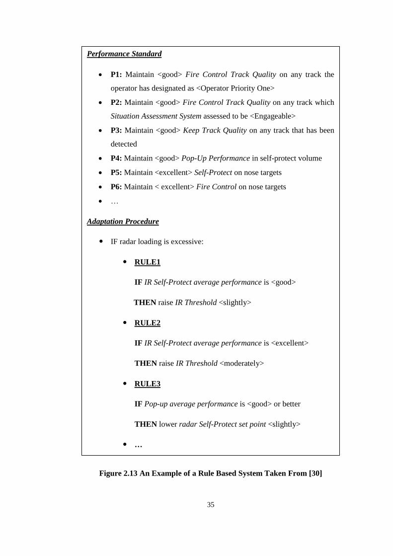
A simple example given in Figure 2.13 for Macro-level rule-based decisions, taken

from [30], is shown below. The example first describes the performance standard

then gives certain rules to satisfy this standard.

35

Figure 2.13 An Example of a Rule Based System Taken From [30]

Performance Standard

P1: Maintain <good> Fire Control Track Quality on any track the

operator has designated as <Operator Priority One>

P2: Maintain <good> Fire Control Track Quality on any track which

Situation Assessment System assessed to be <Engageable>

P3: Maintain <good> Keep Track Quality on any track that has been

detected

P4: Maintain <good> Pop-Up Performance in self-protect volume

P5: Maintain <excellent> Self-Protect on nose targets

P6: Maintain < excellent> Fire Control on nose targets

…

Adaptation Procedure

IF radar loading is excessive:

RULE1

IF IR Self-Protect average performance is <good>

THEN raise IR Threshold <slightly>

RULE2

IF IR Self-Protect average performance is <excellent>

THEN raise IR Threshold <moderately>

RULE3

IF Pop-up average performance is <good> or better

THEN lower radar Self-Protect set point <slightly>

…

36

2.4.3 Optimization-Based Scheduling

Optimization based scheduling assumes a (multi-stage) cost function to be

minimized or a reward function to be maximized over a finite or infinite horizon.

Stochastic optimization methods such as stochastic dynamic programming (SDP) can

be used to determine the optimal radar resource management policy. Unfortunately,

when a large number of states and targets are used, the complexity and the

dimensionality of the DP problem will be huge. In the literature the use of these

techniques are relatively new due to their high computational power requirement

[31], [32] and [33].

In resource management, we desire to optimize a non-instantaneous reward criterion.

A non-instantaneous reward means that future consequences over a finite or infinite

time-horizon are considered when making a decision. Within the time horizon, new

decisions will be made, and this is handled in the modeling by formulating a multi-

stage decision problem.

Unfortunately, in all of the models used for this purpose the size of the state space

explodes exponentially with the number of targets in the scenario, and an optimal

approach is infeasible even for a small number of targets. Therefore, approximate

solutions are needed. In [32] it is suggested to separate the problem into components,

so that each component can be optimized locally (Separation into Subtasks).

In this thesis, we will present hierarchical resource management algorithm for ESA

radars. The resource management problem will be formulated as a constrained

Markov decision process that is detailed in Section 3.2 and macro level of a two-

level (two-timescale) resource management algorithm is presented in Section 3.5.

37

2.5 Dynamic Programming

Dynamic programming is an efficient method to solve recursive optimization

problems. For the MDP described in Section 2.3.5, backward dynamic programming

is applied. The basic idea is to start from the last time of the problem horizon [1 𝑇]

and to find the value of the objective function assuming that the state is ‘𝑖’ at this

time for each ‘𝑖’ . At time 𝑇 − 1 it is again assumed that the state is ‘𝑖’, and the

incremental reward and the expected value of the reward of going from time 𝑇 − 1 to

time 𝑇 is maximized with respect to the input. Detailed explanation of the algorithm

is given below [34], [13].

Let 𝑛 be the time horizon that we try to maximize the expected aggregate reward.

Time interval starts from “𝑚” to “𝑚 + 𝑛 − 1”, [𝑚,𝑚 + 𝑛 − 1], with a final reward

at time 𝑚 + 𝑛. Suppose 𝑛 = 1, decision k is made with instantaneous reward 𝑟𝑖(𝑘),

given 𝑋𝑚 = 𝑖. The next state 𝑋𝑚+1 = 𝑗 with probability 𝑃𝑖𝑗(𝑘) and the final reward is

𝑢𝑗 . The expected aggregate reward over times “𝑚” and “𝑚 + 1”, maximized over the

decision 𝑘, is then

𝑣𝑖∗(1, 𝑢) = max

𝑘{𝑟𝑖

(𝑘) + ∑𝑃𝑖𝑗(𝑘)𝑢𝑗

𝑗

} (2.31)

Note that, only one decision is made at time 𝑚, but there are 2 rewards. One is at

time 𝑚 and the other is the final reward at 𝑚 + 1.

The notation 𝑣𝑖∗(𝑛, 𝑢) is used to represent the maximum expected aggregate reward

from time 𝑚 to 𝑚 + 𝑛 starting at 𝑋𝑚 = 𝑖.

38

With these notation (2.31) become

𝑣∗(1, 𝑢) = max𝑘

{𝑟𝑘 + [𝑃𝑘]𝑢} (2.32)

where 𝑘 = (𝑘1, 𝑘2, … , 𝑘𝑀)𝑇, 𝑟𝑘 = (𝑟1𝑘1 , 𝑟2

𝑘2 , … , 𝑟𝑀𝑘𝑀)𝑇,

Now, consider 𝑣𝑖∗(2, 𝑢) which is the maximum expected aggregate reward starting

from 𝑋𝑚 = 𝑖 with decisions made at times 𝑚 and 𝑚 + 1 and a final reward at

time 𝑚 + 2. An optimal decision at time 𝑚 + 1 can be selected based only on the

state 𝑗 at time𝑚 + 1 . The decision at time 𝑚 + 1 (given𝑋𝑚+1 = 𝑗 ) is optimal

independent of the decision at time 𝑚.

Note that using optimized decision at time m + 1, given 𝑋𝑚 = 𝑖 and decision 𝑘 is

made at time 𝑚 , then the sum of expected rewards at times 𝑚 + 1 and 𝑚 + 2

is ∑ 𝑃𝑖𝑗(𝑘)𝑣𝑗

∗(1, 𝑢)𝑗 . Adding the expected reward at time 𝑚 and maximizing over

decisions at time 𝑚,

𝑣𝑖∗(2, 𝑢) = max

𝑘{𝑟𝑖

(𝑘) + ∑𝑃𝑖𝑗(𝑘)𝑣𝑗

∗(1, 𝑢)

𝑗

} (2.33)

This same argument can be used for all larger numbers of trials. To find the

maximum expected aggregate reward from time 𝑚 to 𝑚 + 𝑛 , we first find the

maximum expected aggregate reward from 𝑚 + 1 to 𝑚 + 𝑛 , conditional

on 𝑋𝑚+1 = 𝑗 for each state 𝑗. This is the same as the maximum expected aggregate

reward from time 𝑚 to 𝑚 + 𝑛 − 1 , which is 𝑣𝑗∗(𝑛 − 1, 𝑢) . This gives us the

general expression for 𝑛 ≥ 2:

39

𝑣𝑖∗(𝑛, 𝑢) = max

𝑘{𝑟𝑖

(𝑘) + ∑𝑃𝑖𝑗(𝑘)𝑣𝑗

∗(𝑛 − 1, 𝑢)

𝑗

} (2.34)

We can also write this in vector form as;

𝑣∗(𝑛, 𝑢) = max𝑘

{𝑟𝑘 + [𝑃𝑘] 𝑣∗(𝑛, 𝑢)} (2.35)

where k is a set of decisions 𝑘 = (𝑘1, 𝑘2, … , 𝑘𝑀)𝑇 each 𝑘𝑖 is the decision for the

state 𝑖. [𝑃𝑘] is the state transition matrix whose 𝑖𝑗𝑡ℎ element is 𝑃𝑖𝑗(𝑘𝑖) and 𝑟𝑘 denotes

a vector whose 𝑖𝑡ℎ element is 𝑟𝑖(𝑘𝑖). The maximization over 𝑘 in (2.35) is really M

separate and independent maximizations; one for each state, i.e., (2.35) is simply a

vector form of (2.34).

The dynamic programming algorithm performs the calculation of (2.34) or (2.35)

iteratively/recursively for n = 1, 2, 3, … . This algorithm is developed by Bellman

[35]. Note that the algorithm is independent of the starting time 𝑚; the parameter 𝑛 is

the number of decisions over the long time horizon that the expected aggregate gain

is optimized. This algorithm provides the optimal dynamic policy for a given final

reward vector 𝑢 and any given time horizon 𝑛.

40

41

CHAPTER 3

3 IMPLEMENTATION

3.1 Problem Statement

Radar sensor scheduling for multi target tracking for ESA radar is realized by a

stochastic dynamic programming based resource allocation algorithm. Sensor

performance is measured by summing target wise utilities over a long time horizon.

Our aim is to solve the macro scheduling problem by using optimization based

methods. The problem is simplified and reduced to efficient tracking of isolated

tracks that are not in the same beam. Searching is not included. The reduced problem

is: for each time period decide on which tracks should be measured. Although the

aim is to solve the simplified problem it is still too complex to solve by using

dynamic programming. So we made several simplifications.

Target is assumed to be tracked by a Kalman filter using constant velocity

model.

Target’s probabilities of detections are constant on the given time horizon and

known.

Targets are already tracked at the beginning of the interval.

42

There is no search function. We deal only with the tracking task.

There is no track initiation process. If a target drops, it will never be re-

initiated.

There is no false alarm.

The multidimensional kinematic state of each target is quantized to a single

Markov chain.

Under these conditions the scheduling problem is formulated as a Markov decision

process. Since the size of the Markov chain increases exponentially with the number

of targets, Lagrange relaxation is applied to dynamic programming to simplify the

state space dimension. The interval of the slow time scale is in the order of seconds.

Macro manager decides which targets will be tracked at each macro time interval

over the time horizon under certain constraints. The sensor performance is

characterized by a target-wise utility function which is called ‘reward function’ of

the target. The macro manager decides to allocate more radar resources to where the

demand is high such as the high priority targets, adaptively.

We present in Section 3.1 the general scenario, target dynamic model that is used and

the objective function that determines the performance. These lead to the

construction of the related Markov chains given in Section 3.1.4. Resource allocation

formulation on the slow timescale as a stochastic optimization problem is given in

Section 3.2 and the resource constraints are defined in Section 3.3. By using

Lagrange relaxation, overall problem can be divided into subtasks. The way we

perform sub task separation is given in Section 3.4 and corresponding algorithm that

is used for implementation is given in Section 3.5.

43

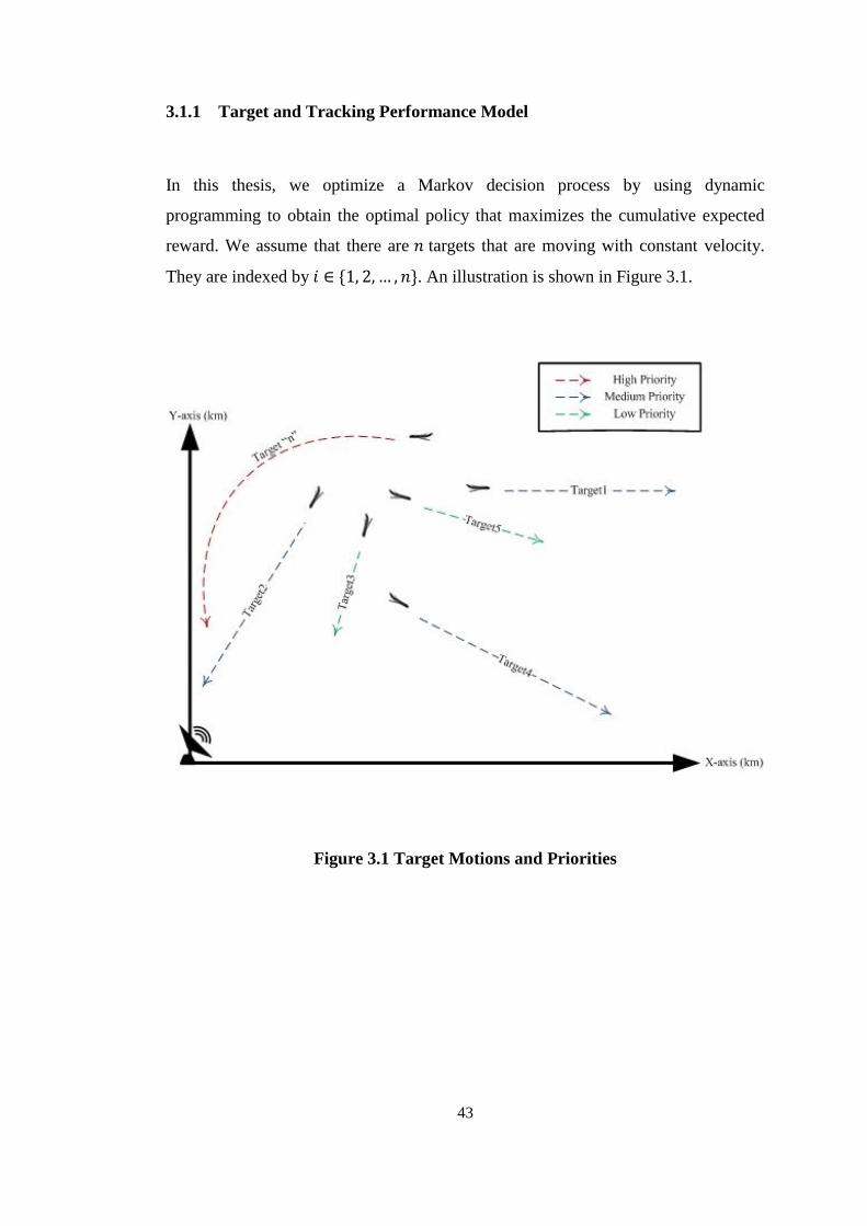
3.1.1 Target and Tracking Performance Model

In this thesis, we optimize a Markov decision process by using dynamic

programming to obtain the optimal policy that maximizes the cumulative expected

reward. We assume that there are 𝑛 targets that are moving with constant velocity.

They are indexed by 𝑖 ∈ {1, 2, … , 𝑛}. An illustration is shown in Figure 3.1.

Figure 3.1 Target Motions and Priorities

44

The target 2-D kinematic states are defined as:

𝜉𝑖(𝑡) = [𝑟𝑥,𝑖(𝑡), 𝑟𝑦,𝑖(𝑡), 𝑣𝑥,𝑖(𝑡), 𝑣𝑦,𝑖(𝑡)]𝑇 (3.1)

where 𝑟𝑥,𝑖(𝑡), 𝑟𝑦,𝑖(𝑡) are the position parameters of the target and 𝑣𝑥,𝑖(𝑡), 𝑣𝑦,𝑖(𝑡) are

the velocity parameters. The linear state space model is defined as:

𝜉𝑖(𝑡 + 𝑇) = 𝐹(𝑇)𝜉𝑖(𝑡) + 𝑤𝑖(𝑇) (3.2)

where 𝐹(𝑇) is the state transition matrix of the target state model and 𝑤𝑖(𝑇) is the

white Gaussian process noise 𝑤𝑖(𝑇)~𝑁(0, 𝑄𝑖(𝑇)).

Measurement model is expressed as:

𝑦𝑖(𝑡) = 𝐶𝜉𝑖(𝑡) + 𝑣𝑖(𝑡) (3.3)

where 𝐶 is the observation matrix of the target state model and 𝑣𝑖(𝑡) is the white

Gaussian measurement noise 𝑣𝑖(𝑡)~𝑁(0, 𝑅𝑖).

For simplicity, Kalman filter is used to evaluate state estimate 𝜉𝑖,𝑡|𝑠(𝑡) of the track of

the target 𝑖 at time 𝑡 given the measurement at time 𝑠. The conditional covariance is

𝑃𝑖,𝑡|𝑠 = 𝐸{𝜉𝑖,𝑡|𝑠 𝜉𝑖,𝑡|𝑠𝑇} (3.4)

45

where 𝜉𝑖,𝑡|𝑠 = 𝜉𝑖(𝑡) − 𝜉𝑖,𝑡|𝑠(𝑡) .

In general, 𝑃𝑖,𝑡|𝑠 is the most important input of the resource allocation process. For

high priority targets, conditional covariance matrix is tried to be minimized. There is

a direct dependence between covariance matrix and how often measurements are

taken from the corresponding target. 𝑄𝑎𝑐𝑐,𝑖(𝑃𝑖,𝑡|𝑠) is derived from covariance matrix

and it is a measure of the accuracy of the corresponding target.

A discrete parameterization of 𝑃𝑖,𝑡|𝑠 that represents the current state accuracy is given

by the Kalman filter when the target is tracked.

3.1.2 Discrete Parameterization of State Rewards

The discrete parameterization of the Kalman filter covariance is presented in this

section. This is needed to specify the state quality at a finite number of discrete

values. Later, reward of a track is related to the discrete parameterization of

covariance matrix.

Note that Kalman filter predicted and corrected covariance equations (2.16) and

(2.18) are given in Section 2.2.2. When no beam is transmitted to the target

according to the policy used, Kalman filter prediction step is applied. On the contrary

if a measurement is taken, the both prediction and correction steps are applied. Two

Markov chains are constructed for update / do not update decisions. The constructed

Markov chains give the quantized accuracy 𝑄𝑎𝑐𝑐,𝑖(𝑃𝑖,𝑡|𝑠) of the next state. To be

more precise let 𝑘𝑛 be the discrete time instance when the observation 𝑛 occurs. Let

𝑇𝑛 = 𝑘𝑛 − 𝑘𝑛−1 be the time between two update decisions. Actually, 𝑇𝑛 refers to the

number of prediction steps. The Kalman filter covariance prediction and correction

steps are progressed according to Riccati equation:

46

Prediction Step:

𝑃𝑖,𝑘𝑛|𝑘𝑛−1= 𝐹(𝑇𝑛)𝑃𝑖,𝑘𝑛−1|𝑘𝑛−1

𝐹(𝑇𝑛)𝑇 + 𝑄𝑖(𝑇𝑛) (3.5)

Correction Step:

𝑃𝑖,𝑘𝑛|𝑘𝑛= (𝐼 − 𝐾𝑖,𝑛𝐻)𝑃𝑖,𝑘𝑛|𝑘𝑛−1

(𝐼 − 𝐾𝑖,𝑛𝐻)𝑇

+ 𝐾𝑖,𝑛𝑅𝑖,𝑛𝐾𝑖,𝑛𝑇

(3.6)

where 𝑄𝑖(𝑇𝑛) is the covariance of the process noise in the constant velocity motion

model, 𝑅𝑖,𝑛 is the covariance of the measurement noise, 𝐾𝑖,𝑛 is the Kalman gain and

𝐻 is the observation matrix.

The trace of covariance matrix is accepted as the state quality. The Markov chain

states correspond to quantized state quality 𝑄𝑎𝑐𝑐,𝑖(𝑃𝑖,𝑡|𝑠) . In our applications the

number of states is 26 meaning that quality is quantized into 25 values and the last

state denotes the track drop. An algorithm is generated for the quantization of the

quality. The algorithm is based on a fixed topology of the Markov chain. A simple

example of a 10-state topology is given in Figure 3.2. The algorithm given in Table

3.1 determines the values of the covariance matrices for each state or equivalently

quality of it according to the fixed topology. The approach of the algorithm is to find

possible covariance matrices for different update/do not update events and then

quantize the corresponding quality. Note that although the decision is for the Markov

chain corresponding to the input ‘update’, due to miss detections, the update event

may not occur. The examples in the pseudo code are for the 10-state example given

in Figure 3.2.

47

Figure 3.2 is constructed so that the quality decreases both as states moves to right

and also down. The best state is State 1 and the smallest possible value of its

covariance matrix is obtained when an update is applied at each time instant. The

steady state covariance matrix gives an upper bound for the quality of this state. A

lower bound is found by considering returns to this state from a state which has

smallest quality. For the Markov chain of Figure 3.2, for initial state 1, this path is 4-

7-3-6-9-3-6-9-3-1 and is obtained as a result of updating event of 0010010011 where

1 corresponds to a measurement update while 0 is only time update. The upper and

lower bounds obtained in this way are used as bounds of quantization levels.

Figure 3.2 A Simple Example of a 10-State Topology

48

A pseudo code for discrete parameterization of state rewards is given in Table 3.1.

Table 3.1 A Pseudo Code for Discrete Parameterization of State Rewards

Apply the following procedure to each state 𝑖.

Assume an initial covariance matrix for state 𝑖.

1) Initialize the Kalman filter

2) Update covariance matrix by processing Kalman filter a few iterations to

reach steady state value of covariance matrix.

3) Find the shortest path that is determined by given update/do not update

decision to reach the same state. (Best case)

As an example,

[1 1 1 1 1 1 1 1 1 1] is the best case decision sequence for state 1.

4) Find the longest path that is determined by given update/do not update

decision to reach the same state. (Worst case)

As an example,

[0 0 1 0 0 1 0 0 1 1] is the worst case decision sequence for state 1.

5) Progress the Kalman filter according to decision sequence

a. ‘0’ means do not update decision and apply only prediction step

b. ‘1’ means update decision and apply both prediction and correction

steps

6) Calculate the trace of Kalman filter covariance matrix for best and worst

case.

7) Best case and worst case are the bounds for quantization of state

uncertainty.

8) Average value of bounds is assumed for the discretized state uncertainty

for the corresponding state.

9) Repeat this procedure for all states.

10) After uncertainties of all states are calculated, normalize them inversely to

obtain state rewards. It means smaller uncertainty gets higher reward.

0 ≤ 𝑄𝑎𝑐𝑐,𝑖(𝑃𝑖,𝑡|𝑠) ≤ 1

49

3.1.3 Tracking Performance Characterization

A finite valued discrete time state 𝑥𝑖,𝑘 is defined for each target ‘𝑖’ . The tracking

performance is determined by these states. ‘𝑘’ is the slow timescale and the macro

manager makes decisions on this slow timescale. At each time instant 𝑘, the state 𝑥𝑖,𝑘

is an aggregate of state variables that are:

𝑥𝑖,𝑡𝑟𝑎𝑐𝑘𝑒𝑑(𝑡) ∈ {0, 1} refers as if a target is tracked or not in the time interval

𝑘.

Current accuracy 𝑄𝑎𝑐𝑐,𝑖(𝑃𝑖,𝑘|𝑘𝑠).

These variables are needed to express the instantaneous utility 𝑈𝑖(𝑥𝑖,𝑘) is defined as:

𝑈𝑖(𝑥𝑖,𝑘) = 𝑈𝑛𝑜𝑚,𝑖𝑄𝑎𝑐𝑐,𝑖(𝑃𝑖,𝑘|𝑘𝑠)𝑥𝑡𝑟𝑎𝑐𝑘𝑒𝑑,𝑖,𝑘(𝑡) (3.7)

In this expression 𝑈𝑛𝑜𝑚,𝑖 is the nominal utility function of the 𝑖𝑡ℎ track, which must

be determined by an external authority such as the operator. That value indicates the

priority level of each target 𝑖. It is assumed that 𝑈𝑛𝑜𝑚,𝑖 is constant during the long

time horizon.

The overall instantaneous utility of the radar system at time 𝑘 is the sum of the

individually defined utility functions that is specified for each target. It is defined as:

𝑈(𝑥𝑘) = ∑𝑈𝑖(𝑥𝑖,𝑘)

𝑀

𝑖=1

(3.8)

𝑥𝑘 = {𝑥𝑖,𝑘}𝑖=1

𝑀 (3.9)

50

where 𝑖 is the index of the target, 𝑘 is the current time instance.

3.1.4 Markov Model Used in the Thesis

In this section, Markov models that are used in this thesis on the slow timescale are

discussed. A controlled Markov chain is constructed for each target and state

transitions are determined by the control action: “update/do not update track”. All

targets have the same controlled Markov chain structure. They differ by state

transition probabilities that depend on detection probability of each target. We

assume that detection probabilities depend on range of the target but do not change in

the optimization interval. States of the Markov chain refer tracking quality that is

determined by kinematic equations of target and derived from target error covariance

matrix by quantizing the trace of the error covariance matrix given by the tracker.

Consider 𝑝𝑥𝑖,𝑘 as the state probability vector of 𝑥𝑖,𝑘. We assume that transitions in

Markov chain depend on the current kinematic state and the measurement decision

(update/do not update). Then, the target-wise dynamic model has the following form,

𝑝𝑥𝑖,𝑘+1= 𝑃𝑡𝑟,𝑖(𝑑𝑘, 𝜉𝑖(𝑡))𝑝𝑥𝑖,𝑘

(3.10)

where 𝑃𝑡𝑟,𝑖 is the transition matrix of the Markov chain.

In our constructed Markov model, each target is represented by a twenty six state

Markov chain. Markov chain states are numbered by considering their quantized

track quality. First state (1) is the best state that has the least trace of the error

covariance matrix. Last state (25) corresponds to the highest uncertainty and state 26

is the drop state that the tracker lost the target. The uncertainty depends on the state

that the last update has occurred and the duration between two consecutive update

instances. If a target is updated, the Markov chain jumps to one of the leftmost states

51

depending on the time 𝑇𝑛 = 𝑘𝑛 − 𝑘𝑛−1 that is the time between the two update

decisions. This means, if two consecutive update decisions are made, Markov chain

jumps first state because of the time between two update decisions is 1. After an

update decision, if two do not update decisions are made and then an update decision

is made, Markov chain jumps two state to the right and jumps to the second state

because of the time between two update decisions is 2.

The constructed update and do not update decisions dependent Markov chains are

shown in Figure 3.3 and Figure 3.4, respectively.

52

Figure 3.3 Target-Wise Markov Chain for Update Decision

53

Figure 3.4 Target-Wise Markov Chain for Do Not Update Decision

54

After we construct the Markov chains, the maximum numbers of looks that are used

for improved detection probability are designed. This is needed because of the

observation that if no such arrangements are done the target drops are excessive.

Different numbers of update attempts are determined by the rule given below.

Main idea: Use less number of looks for better states. Each ‘update’ input triggers a

possible sequence of look oriented to the target. For the case of unavailability of the

observation the procedure is repeated. The number of possible repetitions in this

application is given below for the 26 state Markov chain given in Figure 3.3.

At most 1 look for states from 1 to 5 (the best quality states)

At most 2 looks for states from 6 to 10



At most 5 looks for states from 21 to 25 (the worst quality states)

State transition probabilities are different because of the number of looks used for

repeated update attempts are different. According to the probability of detection a

target may or may not be observed in a single look. At most ‘n’ (n is selected by the

rule given above) looks are reserved for this purpose. The probability of detection of

the target in:

1 look is: 1 − (1 − 𝑃𝑑)

2 looks is: 1 − (1 − 𝑃𝑑)2

3 looks is: 1 − (1 − 𝑃𝑑)3

4 looks is: 1 − (1 − 𝑃𝑑)4

5 looks is: 1 − (1 − 𝑃𝑑)5

55

We assume that 𝑇𝑜𝑛𝑒𝑙𝑜𝑜𝑘 is a fixed parameter refers as the time spent for one look.

As a result the expected time spent to detect a target is calculated by the rule below;

For states from 1 to 5:

o 𝑇𝑜𝑛𝑒𝑙𝑜𝑜𝑘(1. 𝑃𝑑 + (1 − 𝑃𝑑)) if at most one look is allowed.


o 𝑇𝑜𝑛𝑒𝑙𝑜𝑜𝑘(1. 𝑃𝑑 + 2𝑃𝑑(1 − 𝑃𝑑) + 2(1 − 𝑃𝑑)2) if 2 looks are used.


o 𝑇𝑜𝑛𝑒𝑙𝑜𝑜𝑘(1. 𝑃𝑑 + 2𝑃𝑑(1 − 𝑃𝑑) + 3𝑃𝑑(1 − 𝑃𝑑)2) + 3(1 − 𝑃𝑑)3 if 3

looks are used.


o 𝑇𝑜𝑛𝑒𝑙𝑜𝑜𝑘(1. 𝑃𝑑 + 2𝑃𝑑(1 − 𝑃𝑑) + 3𝑃𝑑(1 − 𝑃𝑑)2 + 4𝑃𝑑(1 − 𝑃𝑑)3 +

4(1 − 𝑃𝑑)4) if 4 looks are used.


o 𝑇𝑜𝑛𝑒𝑙𝑜𝑜𝑘(1. 𝑃𝑑 + 2𝑃𝑑(1 − 𝑃𝑑) + 3𝑃𝑑(1 − 𝑃𝑑)2) + 4𝑃𝑑(1 − 𝑃𝑑)3 +

5𝑃𝑑(1 − 𝑃𝑑)4 + 5(1 − 𝑃𝑑)5 if 5 looks are used.

As an example for 𝑃𝑑 = 0.8 the average time spent on the target is 1.24𝑇𝑜𝑛𝑒𝑙𝑜𝑜𝑘, for

states from 11 to 15 and the probability of detection is 0.992 if 3 looks used case.

56

3.2 Resource Allocation Formulation

The tracking performance model and motion model are described in the previous

sections. The objective function and the constraints of the resource allocation

problem are explained here.

The objective function that is used in this thesis, similar to [32], is a utility measure

over a finite or infinite time horizon as desired. So we formulate the problem as a

long horizon planning problem. Long time planning, compared to a myopic policy, is

more advantageous. Long time planning not only includes present utility measure but

also deals with expected future utilities. To achieve that purpose, a non-instantaneous

track utility is defined by integrating the instantaneous utility over a time interval.

𝑈𝑖(𝑡0, 𝑡1) = ∫ 𝑈𝑛𝑜𝑚,𝑖𝑄𝑎𝑐𝑐,𝑖(𝑥𝑖(𝑡))𝑥𝑡𝑟𝑎𝑐𝑘𝑒𝑑,𝑖,𝑘(𝑡)

𝑡1

𝑡0

𝑑𝑡 (3.11)

The current time instant corresponds to 𝑡0 and the time horizon of the decision-

making is [𝑡0, 𝑡1]. In stochastic dynamic programming based problems, the expected

utility refers to an objective function that should be maximized.

𝐸{𝑈𝑖(𝑡0, 𝑡1)|𝑥𝑖(𝑡0)} (3.12)

Now, our aim is to maximize the objective function by making decisions over the

long time horizon. So the objective function is:

𝐽0(𝑥0) = 𝐸 { ∑ 𝑈(𝑥𝑘) | 𝑥0

𝑁−1

𝑘=0

} (3.13)

57

Here, 𝑁 denotes the decision interval. The expectation includes the future radar

measurements. The DP solution reduces the optimization problem to a nested set of

smaller problems given in the recursive form. At time 𝑡0 the optimization problem

can be written as:

max 𝑑0

𝑈(𝑥0) +𝐸 𝑥1| 𝑥0, 𝑑0{ 𝐽1

∗(𝑥1)} (3.14)

where 𝐽1∗(𝑥1) represents the future utility as a consequence of decisions 𝑑0 made at

𝑘 = 0, and given a sequence of optimal future decision, i.e.,

𝐽𝑘∗(𝑥𝑘) = max

𝑑𝑘

𝑈(𝑥𝑘) +𝐸 𝑥𝑘+1| 𝑥𝑘, 𝑑𝑘{ 𝐽𝑘+1

∗(𝑥𝑘+1)} (3.15)

The decisions are assumed to fulfill the resource constraints on available

measurement time. Note that in the above equation, the modeling of the objective

function has a recursive form of nested maximizations and expectations.

3.3 Resource Constraints

The randomness of the actual execution time of tracking a target task constraint the

radar resources to allocate them in an efficient way. It is assumed that 𝑇𝑜𝑛𝑒𝑙𝑜𝑜𝑘 is

defined as the time spent for one look. To track a target, the number of looks used is

also random that depends on each targets current state in Markov chain as described

in Section 3.1.4. All states are parameterized due to expected consuming resources

according to the quality of each state. States in Markov chain are grouped into

corresponding columns and each column has a different expected number of looks to

track a target. Looks that are planned to track a target are expectedly allocated in a

58

rule based fashion described in Section 3.1.4. According to this rule, expected loads

of each state can be calculated. This load is called as state dependent load and it is

used in dynamic programming. After the optimal strategy is obtained, we check the

time dependent load. The sum of time dependent load should be equal or less than 1

which describes the percentage load of each slow time interval.

𝑙𝑘(𝑥𝑘, 𝑑𝑘) = 𝐸{𝑙𝑘(𝑥𝑘, 𝑑𝑘)|𝑥𝑘, 𝑑𝑘} ≤ 1 (3.16)

3.4 Separation into Subtasks

The problem and the corresponding stochastic dynamic programming solution given

in (3.17) is a Markov decision process with a very large number of states even for

few targets. Unfortunately, stochastic dynamic programming becomes harder while

the number of states in state spaces is increasing as it is shown in Section 4.3 and

Section 4.4. To solve the problem the Lagrange relaxation method, given in [32] is

applied to the problem. The formulation here is taken from [32]. This formulation

uses some approximations on the formulation. Approximate relaxation of resource

constraints are investigated by Lagrange multipliers. Lagrange relaxation provides us

to separate the problem into components that is described in this section.

Instead of optimizing the global complex stochastic control problem, the problem is

separated into components and optimized locally. Then optimized components are

collected together by the resource constraints given in (3.16). In this thesis, each

tracking task is recognized as a sub problem. The overall system performance at time

𝑘 is the sum of each subtask’s utility.

𝑈(𝑥𝑘) = ∑ 𝑈𝑠(𝑥𝑠,𝑘)𝑠

(3.17)

59

The resource constraints (total load) in the interval 𝑘 is also described by the sum of

the expected load of all subtasks,

𝑙𝑘(𝑥𝑘, 𝑑𝑘) = ∑ 𝑙𝑠,𝑘(𝑥𝑠,𝑘, 𝑑𝑠,𝑘)𝑠

= ∑ 𝐸{𝑙𝑠,𝑘(𝑥𝑠,𝑘, 𝑑𝑠,𝑘)|𝑥𝑠,𝑘, 𝑑𝑠,𝑘}𝑠

≤ 1

(3.18)

By Lagrange relaxation, the constraints are added to the objective function in the

optimization problem.

𝐿𝑘(𝑥𝑘, 𝑑𝑘, 𝜆𝑘)

= 𝑈(𝑥𝑘) + 𝜆𝑘 (1 − 𝑙𝑘(𝑥𝑘 , 𝑑𝑘))

+ 𝐸𝑥𝑘+1|𝑥𝑘,𝑑𝑘{max𝑑𝑘+1

𝐿𝑘+1(𝑥𝑘+1, 𝑑𝑘+1, 𝜆∗𝑘+1(𝑥𝑘+1))}

(3.19)

where 𝜆𝑘 corresponds the Lagrange multiplier at time 𝑘 and 𝜆𝑘∗(𝑥𝑘) is the Lagrange

multiplier that the resource constraint is fulfilled with equality at optimum decisions

at time 𝑘. The optimal Lagrangian at time 𝑘, 𝐿𝑘(𝑥𝑘, 𝑑𝑘∗(𝑥𝑘), 𝜆𝑘

∗(𝑥𝑘)) is equal to the

optimal value-to-go function 𝐽𝑘∗(𝑥𝑘). At the end of long time interval 𝑁, Lagrangian

is equal to utility.

𝐿𝑁(𝑥𝑁) = 𝑈(𝑥𝑁) (3.20)

60

At time 𝑘 the Lagrangian expression can be written as

𝐿𝑘(𝑥𝑘, 𝑑𝑘, 𝜆𝑘)

= ∑ 𝑈𝑠(𝑥𝑠,𝑘)𝑠

+ 𝜆𝑘 (1 − ∑ 𝑙𝑠,𝑘(𝑥𝑠,𝑘, 𝑑𝑠,𝑘)𝑠

)

+ 𝐸𝑥𝑘+1|𝑥𝑘,𝑑𝑘{max

𝑑𝑘+1

∑ 𝑈𝑠(𝑥𝑠,𝑘+1)𝑠

+ 𝜆𝑘+1∗(𝑥𝑘+1) (1 − ∑ 𝑙𝑠,𝑘+1(𝑥𝑠,𝑘+1, 𝑑𝑠,𝑘+1)

𝑠)

+𝐸𝑥𝑘+2|𝑥𝑘+1,𝑑𝑘+1{max𝑑𝑘+2

𝐿𝑘+2(𝑥𝑘+2, 𝑑𝑘+2, 𝜆∗𝑘+2(𝑥𝑘+2))}}

(3.21)

Rearranging the terms gives

𝐿𝑘(𝑥𝑘, 𝑑𝑘 , 𝜆𝑘)


− 𝜆𝑘𝑙𝑠,𝑘(𝑥𝑠,𝑘, 𝑑𝑠,𝑘) + 𝜆𝑘


∑ 𝑈𝑠(𝑥𝑠,𝑘+1)𝑠

− 𝜆𝑘+1∗(𝑥𝑘+1)𝑙𝑠,𝑘+1(𝑥𝑠,𝑘+1, 𝑑𝑠,𝑘+1)

+𝐸𝑥𝑘+2|𝑥𝑘+1,𝑑𝑘+1{max𝑑𝑘+2

𝐿𝑘+2(𝑥𝑘+2, 𝑑𝑘+2, 𝜆∗𝑘+2(𝑥𝑘+2))}

+ 𝜆𝑘+1∗(𝑥𝑘+1)}

(3.22)

A separation of (3.22) in terms of subtasks requires that the inner sums to be moved

to the outside of both the maximizations and the expectations. In these expressions,

𝜆𝑘∗(𝑥𝑘) is a function of the global state, and this prevents the separation. However, it

is assumed that the variation of 𝜆𝑘∗(𝑥𝑘) is moderate compared with the

61

average 𝐸𝑥𝑘|𝑥0{𝜆𝑘

∗(𝑥𝑘) }. It is then reasonable to replace 𝜆𝑘∗(𝑥𝑘) for 𝑘 > 0 with its

estimates. These estimates are denoted �̂�𝑘∗, and are chosen such that

𝐸𝑥𝑘|𝑥0 {𝑙𝑘(𝑥𝑘, 𝑑𝑘∗(𝑥𝑘))} = 1, 𝑘 > 0. (3.23)

It will be a part of a global optimization algorithm to search for �̂�𝑘∗. It is said that the

long term variation of the Lagrange multipliers typically depends on the number of

tracked targets [32].

For notational convenience, define the vector of Lagrange multiplier estimates as

�̃� = [�̃�0, �̂�1∗, �̂�2

∗, … , �̂�𝑁−1

∗] and denote the element corresponding to time 𝑘 as �̃�𝑘.

Assume that the Lagrangian at time 𝑘 + 1 can be rewritten as a sum of Lagrange

components for each subtask, plus a term depending on the multipliers only,

𝐿𝑘(𝑥𝑘 , 𝑑𝑘, �̃�) = ∑ 𝐿𝑠,𝑘(𝑥𝑠,𝑘, 𝑑𝑠,𝑘, �̃�)𝑠

+ ∑ �̃�𝑛

𝑁−1

𝑛=𝑘

(3.24)

The Lagrangian at time 𝑘 is also expressed as

𝐿𝑘(𝑥𝑘, 𝑑𝑘, �̃�)


− �̃�𝑘𝑙𝑠,𝑘(𝑥𝑠,𝑘, 𝑑𝑠,𝑘) + �̃�𝑘


∑ 𝐿𝑠,𝑘+1(𝑥𝑠,𝑘+1, 𝑑𝑠,𝑘+1, �̃�)𝑠

}

+ ∑ �̃�𝑛

𝑁−1

𝑛=𝑘

(3.25)

62

The maximum operation is separable in the subtasks due to the local influence of

decision parameters in subtasks, e.g., if 𝑓𝑠( 𝑑𝑠) is a set of functions representing local

consequences of the decision 𝑑𝑠 regarding measurements of subtask 𝑠, we have that

max𝑑

∑ 𝑓𝑠( 𝑑𝑠)𝑠

= ∑ max𝑑𝑠𝑠

𝑓𝑠( 𝑑𝑠) (3.26)

Thus, the sum can be moved outside the maximization. Furthermore, the expectation

is carried out per subtask due to the independence assumptions regarding target-wise

performance. Consequently, given the assumption in (3.24), the Lagrangian at stage

𝑘 is also separable in the subtasks:

𝐿𝑘(𝑥𝑘 , 𝑑𝑘, �̃�)


− �̃�𝑘𝑙𝑠,𝑘(𝑥𝑠,𝑘, 𝑑𝑠,𝑘)


∑ 𝐿𝑠,𝑘+1(𝑥𝑠,𝑘+1, 𝑑𝑠,𝑘+1, �̃�)𝑠

}

+ ∑ �̃�𝑛

𝑁−1

𝑛=𝑘

≜ ∑ 𝐿𝑠,𝑘(𝑥𝑠,𝑘, 𝑑𝑠,𝑘, �̃�)𝑠

+ ∑ �̃�𝑛

𝑁−1

𝑛=𝑘

(3.27)

At the end of long time horizon, we have 𝐿𝑁(𝑥𝑁) = ∑ 𝑈𝑠(𝑥𝑠,𝑘)𝑠 ≜ 𝐿𝑠,𝑁(𝑥𝑠,𝑁). We

apply dynamic programming in backward and perform a recursive process from time

𝑁. By the way, the Lagrangian at the decision time instant k = 0 separates in the

subtasks. In [36] a similar approximate DP approach is given as an example of

optimizing target classifications.

63

The overall optimization problem is divided into several sub problems that are

optimized locally by using Lagrange multipliers. Each Lagrange multiplier can be

found iteratively to fulfill the resource constrains. But we have to give an initial

value for each Lagrange multiplier to find the optimal value of Lagrangian. Initial

value of each Lagrange multiplier is selected as very large so that the constraint is

not satisfied. Then we begin to decrease Lagrange multipliers until the constraint is

satisfied partially. After that, optimal Lagrange multipliers are calculated in two

different ways.

First method: We have used the ‘fminsearch’ function of MATLAB,

Second method: Iterative solution of new search function that is described below.

�̃�𝑗+1 = �̃�𝑗 + ∆�̃�𝑗 (3.28)

𝐸{𝑙𝑗} +

𝜕𝐸{𝑙𝑗}

𝜕�̃�∆�̃�𝑗 = 1 (3.29)

The expected load coming from the subtask is computed based on optimal update/do

not update decisions and 𝐸{𝑙𝑗} is calculated by summing over all subtasks.

Furthermore, 𝜕𝐸{𝑙𝑗}

𝜕�̃� is summed from the partial derivatives of each subtask. The

corresponding partial derivative of each term is computed numerically. The

numerical procedure computes the objective function for �̃� and �̃� + ∆�̃�𝑗 and

computes the derivative by using the difference in the values. Then, above equations

(3.28) and (3.29) are used to generate the new �̃�.

A pseudo code for searching optimal Lagrange multipliers is formulated in Table 3.2.

64

Table 3.2 Pseudo Code for Searching Optimal Lagrange Multipliers

1) Initiate all Lagrange multipliers from a large value and decrease until the

resource constraint is satisfied.

2) Solve dynamic programming via these Lagrange multipliers

3) Select the Lagrange multiplier that exceeds the resource constraint by a

higher value than others.

4) Decrease the selected Lagrange multiplier by a small value ∆�̃� and solve

dynamic programming again.

5) Subtract new output (state independent load) from the old one and find each

change in state independent load with respect to ∆�̃�.

6) Divide ∆�̃� to each change in state independent load and find new change

value that we will apply to the dynamic programing.

7) Repeat this until all outputs converges to one and never exceed.

The optimal strategy specifies the update or do not update decisions for each target in

each interval and it is dependent on the current states of targets. An update command

triggers one or more update attempts due to the quality of the target’s current state.

This rule is defined in Section 3.1.4. Update attempts may result with success or fail

depend on probability of detection.

3.5 Algorithm

The aim of Markov decision process is to find a decision policy that can be

represented as a matrix that relates the states to the decisions.

“decision_depends_on_states” matrix specifies the action that the decision maker

chooses depending on the current state. The objective is to generate an optimal

policy that will maximize the random reward in a finite time horizon.

65

Now, we define the calculation of the Lagrangian for adaptive target tracking task.

All subtasks have the same form since we deal with only track updates. Equation

(3.27) forms a base for dynamic programming. Resource constraints are included by

the Lagrange multipliers. The Markov decision process is also defined in this section.

Let tracking a target 𝑇𝑖 be a sub task and 𝐽𝑖,𝑘(𝑥𝑖,𝑘) be the value-to-go function for 𝑇𝑖

at time 𝑘. 𝐽𝑖,𝑘(𝑥𝑖,𝑘) can be defined as the local Lagrangian of the sub task given the

Lagrange multiplier vector �̃�.

𝐽𝑖,𝑘(𝑥𝑖,𝑘) = 𝐿𝑇𝑖,𝑘(𝑥𝑖,𝑘, 𝑑𝑖,𝑘, �̃�) (3.30)

Given �̃�, the local decision problem is characterized as a Markov decision process.

The solution of the optimization is achieved by dynamic programming backward

recursions.

𝐽𝑖,𝑘∗(𝑥𝑖,𝑘)

= max𝑑𝑖,𝑘

(𝑈𝑖(𝑥𝑖,𝑘) − �̃�𝑘𝑙𝑖,𝑘(𝑥𝑖,𝑘, 𝑑𝑖,𝑘)

+ ∑ 𝐽𝑖,𝑘+1∗(𝑥𝑖,𝑘+1)𝑃(𝑥𝑖,𝑘+1|𝑥𝑖,𝑘, 𝑑𝑖,𝑘, 𝜉𝑖,𝑘)

𝑥𝑖,𝑘+1

)

(3.31)

Here, 𝐽𝑖,𝑁 = 𝑈𝑖(𝑥𝑖,𝑁) and 𝑙𝑖,𝑘(𝑥𝑖,𝑘, 𝑑𝑖,𝑘) is the expected load given a scheduled track

update, and given the filter covariance predicted by the state in time interval 𝑘. Since

the decision can be update or do not update, 𝑙𝑖,𝑘(𝑥𝑖,𝑘, 𝑑𝑖,𝑘) is zero when the decision

is do not update. At each time and state a comparison is done and the maximum of

result that is between update or do not update decisions is chosen.

66

∑ 𝐽𝑖,𝑘+1∗(𝑥𝑖,𝑘+1)𝑃(𝑥𝑖,𝑘+1|𝑥𝑖,𝑘, 𝑑𝑢𝑝𝑑𝑎𝑡𝑒 , 𝜉𝑖,𝑘)

𝑥𝑖,𝑘+1

− ∑ 𝐽𝑖,𝑘+1∗(𝑥𝑖,𝑘+1)𝑃(𝑥𝑖,𝑘+1|𝑥𝑖,𝑘, 𝑑𝑑𝑜_𝑛𝑜𝑡_𝑢𝑝𝑑𝑎𝑡𝑒 , 𝜉𝑖,𝑘)

𝑥𝑖,𝑘+1

(3.32)

This value compared with the cost of update decision �̃�𝑘𝑙𝑖,𝑘(𝑥𝑖,𝑘, 𝑑𝑢𝑝𝑑𝑎𝑡𝑒). Update

decision is given when the reward is larger than the cost.

A pseudo code for separated solution to resource allocation is formulated in Table

3.3.

67

Table 3.3 Pseudo Code for the Separated Solution to Resource Allocation

Assume that an initial estimate of �̃� exists and then an algorithm for generating a

measurement batch is now the following.

1) Form subtasks: Each tracked target forms a subtask.

2) Construct the Markov Model

3) Calculate the expected time spent for each state

4) Initialize all parameters that are input from the operator.

a. Probability of Detection for each target (𝑃𝑑)

b. Nominal utility (𝑈𝑛𝑜𝑚) =100

c. Time horizon (𝑁) =10 sec

d. Initial estimate of �̃�

e. Number of Monte Carlo simulation = 1000

5) Calculate the utilities of each state for each target

6) Calculate the state dependent expected load for each target

7) Apply backwards recursive DP to obtain the optimal strategy for each

tracked target

8) Form the initial state probability vector at time 𝑘 = 0 to initialize the state

9) Calculate 𝐸 {𝑙𝑠𝑗} and

𝜕𝐸{𝑙𝑠𝑗}

𝜕�̃� for each subtask

10) Sum 𝐸 {𝑙𝑠𝑗} and

𝜕𝐸{𝑙𝑠𝑗}

𝜕�̃� over the subtasks to calculate 𝐸{𝑙𝑗} and

𝜕𝐸{𝑙𝑗}

𝜕�̃�

11) Update the Lagrange multiplier vector �̃�, according to (3.28) and (3.29)

12) If total state independent load is sufficiently close to one for all time

intervals, proceed to 13, otherwise continue with 7.

13) Run Monte Carlo simulations to observe the number of updates and the

average number of drops for each target and also number of coincidence for

overloads.

69

CHAPTER 4

4 SIMULATIONS AND RESULTS

In this section, we give several scenarios and their corresponding experimental

results. The problems attempted in this study are a set of problems that start from the

simplest one. We call them the ‘scenarios’. The first scenario is a single target. DP

based solution is feasible for a single target. The Markov model of this scenario was

a simplified model. The performance of the algorithm is tested on this simple model

as described in Section 4.1. 1000 Monte Carlo runs are done on this simple model to

observe the number of updates and the average number of drops. Results show that

the number of target drops is high. Therefore, the model is modified to include some

rules which describe the expected number of looks used in each macro level decision

interval depending on the target’s current state. By this way, the number of drops is

decreased as shown in Section 4.2. The extension of the method to even two targets

needs a very large state space. DP based solution for more than one target is almost

infeasible because of this very large state space. A simple two target example, given

in Section 4.3 is solved by the joint Markov model that gives the optimal solution.

This solution is used as reference to evaluate the results obtained with some

approximations. Section 4.4, the same problem is solved by using Lagrangian

method. Then, in Section 4.5, following approach of [32], the problem is solved by

using a single Markov chain for each target and writing the time budget as a

constraint for eight targets. The constraint optimization problem is solved by using

70

Lagrange relaxation. Lagrange relaxation is the key point of separating the problem

into sub problems. As a result, the exponential explosion of the state space can be

handled.

4.1 DP-Based Optimal Resource Allocation for One Target

In this part, there are some simulations that we have made to observe the usage of

optimal radar resource instead of consuming all resource to one target by using

dynamic programming algorithm. By this way, we can show how to use radar

resources in an efficient way. The Markov chain is the same as the model defined in

Section 3.1.4 except the state transition probabilities. For this scenario, we assume

that each state consumes only one look in Markov decision process instead of the

rule defined in Section 3.1.4. Therefore, state transitions are the same for all states

and it is a constant value that is given by the operator. A cost for update decision is

added to the dynamic programming to avoid the update decisions at all time

intervals. The cost can be selected by the operator. We assume that the utility of do

not update decision is 5 times greater than the utility of update decision. Inputs that

are selected by the operator are given below:

Probability of detection (𝑃𝑑) = 0.8 and 0.4

Nominal utility (𝑈𝑛𝑜𝑚) =100

Time horizon (𝑁) =10 sec

Number of Monte Carlo simulation = 1000

The trace of covariance matrix of each state is calculated by Kalman filter

and ‘state_cov_value’ vector that has the trace of covariance matrix of each

state is constructed. This vector and corresponding normalized vector are

defined below.

71

Quantized values of the state quality defined in Chapter 3.1.2 are given in Table 4.1.

Table 4.1 Quantized Values of the State Quality

State no: 1 2 3 4 5 6 7 8 9 10 11 12 13 Unit

State

Quality 15 18 21 23 25 30 33 36 37 40 58 62 64 m

2

State no: 14 15 16 17 18 19 20 21 22 23 24 25 26 Unit

State

Quality 65 69 101 105 109 112 116 165 173 175 178 181 0 m

2

These values are converted to a reward by the assumption that the reward of the first

state (1) is 1 and the last state (26) is 0. Normalized state rewards are shown in Table

4.2.

Table 4.2 Normalized State Rewards

State no: 1 2 3 4 5 6 7 8 9

State

Rewards 1.000 .8333 .7143 .6522 .6000 .5000 .4545 .4167 .4054

State no: 10 11 12 13 14 15 16 17 18

State

Rewards .3750 .2586 .2419 .2344 .2308 .2174 .1485 .1429 .1376

State no: 19 20 21 22 23 24 25 26

State

Rewards .1339 .1293 .0909 .0867 .0857 .0843 .0829 0.000

The optimum solution provided by the dynamic programming algorithm is given in

Table 4.3. In the table ‘0’ and ‘1’ indicates ‘Do not Update’ and ‘Update’ decision,

respectively.

72

Table 4.3 The Strategy of First Scenario

State no: 𝒕𝟏 𝒕𝟐 𝒕𝟑 𝒕𝟒 𝒕𝟓 𝒕𝟔 𝒕𝟕 𝒕𝟖 𝒕𝟗 𝒕𝟏𝟎

1 0 0 0 0 0 0 0 0 0 0

2 0 0 0 0 0 0 0 0 0 0

3 0 0 0 0 0 0 0 0 0 0

4 0 0 0 0 0 0 0 1 0 0

5 0 0 0 0 0 0 0 1 1 0

6 1 1 1 1 1 1 1 1 1 0

7 1 1 1 1 1 1 1 1 1 0

8 1 1 1 1 1 1 1 1 1 0

9 1 1 1 1 1 1 1 1 1 0

10 1 1 1 1 1 1 1 1 1 0

11 1 1 1 1 1 1 1 1 1 0

12 1 1 1 1 1 1 1 1 1 0

13 1 1 1 1 1 1 1 1 1 0

14 1 1 1 1 1 1 1 1 1 0

15 1 1 1 1 1 1 1 1 1 0

16 1 1 1 1 1 1 1 1 1 0

17 1 1 1 1 1 1 1 1 1 0

18 1 1 1 1 1 1 1 1 1 0

19 1 1 1 1 1 1 1 1 1 0

20 1 1 1 1 1 1 1 1 1 0

21 1 1 1 1 1 1 1 1 1 1

22 1 1 1 1 1 1 1 1 1 1

23 1 1 1 1 1 1 1 1 1 1

24 1 1 1 1 1 1 1 1 1 1

25 1 1 1 1 1 1 1 1 1 1

26 0 0 0 0 0 0 0 0 0 0

After the optimum strategy is obtained, 1000 Monte Carlo simulations are done to

observe the number of updates and the average number of drops. Two different

probability of detection values are used to show relation between 𝑃𝑑 value and

simulation results. Simulation results are given in Table 4.4.

73

Table 4.4 Simulation Results of DP-Based Optimal Resource Allocation for One

Target

𝑷𝒅 = 0.8 𝑷𝒅 = 0.4

Initial

State

Number of

Update in

10 sec.

Number of

average drop in

1000 simulations

Number of

Update in

10 sec.

Number of

average drop in

1000 simulations

1 4.6720 4 3.7030 395

2 4.6120 3 4.6580 370

3 4.6400 10 4.6610 367

4 4.6420 5 4.7050 370

5 4.6550 8 4.6490 366

6 5.2950 7 4.4150 428

7 5.2950 6 5.3230 381

8 5.3140 9 5.2870 376

9 5.2760 6 5.3160 385

10 5.2840 5 5.2790 399

11 5.2600 13 4.8910 429

12 5.2490 10 4.9820 443

13 5.2680 15 4.8700 455

14 5.2530 11 4.9660 451

15 5.2700 12 4.8490 454

16 5.1170 46 4.0710 544

17 5.1470 37 4.0620 558

18 5.1110 44 4.0250 571

19 5.1250 41 4.0870 579

20 5.1210 43 4.0360 570

21 4.4050 192 2.5340 743

22 4.3540 200 2.6560 724

23 4.3280 207 2.6510 735

74

Table 4.4 (cont'd)

24 4.2660 220 2.6780 744

25 4.2580 226 2.5910 733

AVERAGE 4.9287 55.2 4.2378 502.8

These results are obtained by an algorithm that is described by the pseudo code given

in Table 4.5.

Table 4.5 Pseudo Code for DP-Based Optimal Resource Allocation for One

Target

To obtain optimum strategy:

Determine the state transition matrices for update and do not update decisions

Determine the rewards for update and do not update decisions

Apply dynamic programming algorithm

Calculate the corresponding reward for update decision and calculate each

state transition at time N

Calculate the corresponding reward for do not update decision and calculate

each state transition at time N

Compare rewards and select the highest value for each state

Store the highest reward values and corresponding state

Do this procedure for time N-1 to time 0.

To obtain number of updates and drops:

Define an initial state.

Check the optimal decision(update/do not update) from the constructed strategy

If the decision is do not update, change state due to the do not update state

transition matrix

75

Table 4.5 (cont'd)

If the decision is update;

Generate a random variable between zero and one.

If this random variable is less than probability of detection value, change

state due to the do not update state transition matrix

If this random variable is equal or greater than probability of detection

value, change state due to the update state transition matrix

Calculate the number of update decisions and dropped targets that are at the state

26.

The macro manager decision period is 1 sec as the same as Markov decision period.

The simulation time is 10 sec and only one look is used for tracking the target at each

time instant and at each state. In 10 sec, target is tracked nearly five times in the

average. So, simulation results show that we can track one target in an acceptable

uncertainty level by consuming only %50 of the resources nearly. By this

optimization, remaining resource can be used for other tasks such as tracking another

target or may be searching a sector for new targets. The update and drop numbers

depend on the initial state.

4.2 Modified DP-Based Optimal Resource Allocation for One Target with a

Rule

In the previous section, we observed that the number of target drops is quite high.

Therefore, we decide to define a rule for each state. This rule characterizes the

expected usage of looks related to the state quality as described in Section 3.1.4. The

same strategy and inputs are used for this scenario to compare fairly. Simulation

results are given in Table 4.6.

76

Table 4.6 Simulation Results of Modified DP-Based Optimal Resource

Allocation for One Target with a Rule

𝑷𝒅=0.8 𝑷𝒅=0.4

Initial

State

Number of

Update in

10 sec.

Number of

average drop in

1000 simulations

Number of

Update in

10 sec.

Number of

average drop in

1000 simulations

1 4.9890 0 6.4140 2

2 4.9740 0 6.8990 5

3 4.9980 0 7.0560 6

4 5.0170 0 7.0830 6

5 5.0080 0 7.2230 7

6 6.0210 0 7.2500 13

7 6.0360 0 8.2060 8

8 6.0290 0 8.2290 10

9 6.0120 0 8.1210 9

10 6.0040 0 8.1400 12

11 6.0840 0 8.4010 9

12 6.0300 0 8.3450 11

13 6.0760 0 8.3980 13

14 6.0500 0 8.4270 7

15 6.0770 0 8.4510 13

16 6.0710 0 8.3500 14

17 6.0880 0 8.5620 16

18 6.0740 0 8.4430 17

19 6.0810 0 8.3270 17

20 6.0690 0 8.2810 15

21 6.1010 0 8.0970 62

22 6.0990 0 8.0980 72

23 6.1170 0 7.9950 74

77

Table 4.6 (cont'd)

24 6.0640 1 7.9790 84

25 6.1030 1 8.0930 81

AVERAGE 5.8509 0.08 7.9547 23.32

By this rule, we reduce the number of target drops significantly. The reason of zero

drops at states from 1 to 23 is the high probability of detection value. It is chosen as

0.8 same as the previous scenario. If we decrease this value, we will observe track

drops as expected. At the same time, obviously the expected value of the update time

is larger than the previous one. To show the relation between probability of detection

value and the number of target drops, additional columns are added to the Table 4.4

and Table 4.6. Actually, added rule changes the optimal strategy. But this affect is

not significant. So, for fair comparison, we use the same optimal strategy.

4.3 Optimization-Based Resource Allocation for Two Targets

DP based solution for more than one target is almost infeasible because of its very

large state space. However to assess the approximation done for more realistic

problems at this section we generate a new scenario of two targets with a simpler

Markov model. Because of the size of the state space increases exponentially with

the number of targets and the number of states used in the scenario, we consider a

very simple example to obtain the optimal solution. The Markov chain structure of

this scenario is given in Figure 4.1.

78

Figure 4.1 A Simple Markov Model of Each Target

Aim is to obtain the optimal strategy by using the joint Markov model. We have only

one look at each time instant and determine a policy that maximizes the overall

system performance. To achieve this purpose, we need to construct another Markov

model that represents joint situations of the targets. The joint Markov model consists

of 16 states that are the combination the individual Markov model of two targets.

Figure 4.2 shows joint transitions with respect to update decisions of target 1, Figure

4.3 shows joint transitions with respect to update decisions of target 2 and Figure 4.4

shows joint transitions with respect to do not update decision of both targets. Inputs

that are selected are given below:

Probability of detection for target 1(𝑃𝑑1) = 0.8

Probability of detection for target 2 (𝑃𝑑2) = 0.7

Nominal utility for target 1 (𝑈𝑛𝑜𝑚1) = 100


Time horizon (𝑁) = 10 sec


79

Figure 4.2 Joint Markov Model with Respect to Update Decisions of Target 1

Figure 4.3 Joint Markov Model with Respect to Update Decisions of Target 2

80

Figure 4.4 Joint Markov Model with Respect to do not Update Decision of Both

Targets

Each joint state is defined in Table 4.7. It means,

If target 1 is in state 1 and target 2 is in state 1, the joint state will be in state

1, or

If target 1 is in state 2 and target 2 is in state 3, the joint state will be in state

7, and so on.

81

Table 4.7 Joint State Space Representation for Two Targets with Four

Individual State Markov Model

First

Target's

State

Second

Target's

State

Joint State

Normalized

State Quality

Value

1 1 1 100

1 2 2 90

1 3 3 70

1 4 4 15

2 1 5 90

2 2 6 80

2 3 7 50

2 4 8 10

3 1 9 70

3 2 10 50

3 3 11 30

3 4 12 5

4 1 13 15

4 2 14 10

4 3 15 5

4 4 16 0

After the dynamic programming algorithm is applied, optimum decisions are

obtained as the output of DP. 𝑡𝑖 is the time instances of decision horizon. State no

column describes the joint state number. Table 4.8 shows the optimal decisions at

each time instance 𝑡𝑖. “0” means do not update any target, “1” means update target 1

and “2” means update target 2.

82

Table 4.8 An Example of Optimized Policy for Joint Markov Model


1 1 1 1 1 1 1 1 1 2 1

2 2 2 2 2 2 2 2 2 2 2

3 2 2 2 2 2 2 2 2 2 2

4 1 1 1 1 1 1 1 1 1 1

5 1 1 1 1 1 1 1 1 1 1

6 1 1 1 1 1 1 1 1 1 1

7 2 2 2 2 2 2 2 2 2 2

8 1 1 1 1 1 1 1 1 1 1

9 1 1 1 1 1 1 1 1 1 1

10 1 1 1 1 1 1 1 1 1 1

11 1 1 1 1 1 1 1 1 1 1

12 1 1 1 1 1 1 1 1 1 1

13 2 2 2 2 2 2 2 2 2 2

14 2 2 2 2 2 2 2 2 2 2

15 2 2 2 2 2 2 2 2 2 2

16 0 0 0 0 0 0 0 0 0 0

After the optimum strategy is obtained, 1000 Monte Carlo simulations are run to

observe the number of update decisions and the average number of drops for each

target. Simulation results are given in Table 4.9.

83

Table 4.9 Simulation Results of Optimal Resource Allocation for Joint Markov

Model

Target1

𝑷𝒅𝟏 =0.8

Target2

𝑷𝒅𝟐 =0.7

Initial

State

Number of

Update in

10 sec.

Number of

average drop in

1000 simulations

Number of

Update in

10 sec.

Number of

average drop in

1000 simulations

1 5.4820 180 4.2050 365

2 4.6740 216 4.9490 365

3 5.9270 140 3.8390 508

4 9.8450 39 0.0000 1000

5 5.2660 239 4.3610 387

6 6.6830 171 2.8190 600

7 4.8680 323 4.4560 473

8 9.4550 93 0.0000 1000

9 4.2940 377 5.2250 308

10 5.2700 311 4.0300 477

11 8.0290 242 0.0000 1000

12 8.2770 209 0.0000 1000

13 0.0000 1000 9.4750 128

14 0.0000 1000 8.9330 192

15 0.0000 1000 7.1280 367

AVERAGE 5.2047 369.3 3.9613 544.6

Number of states of the joint Markov chain is increasing exponentially with the

number of targets. If the joint Markov model is used to find optimal strategy, we will

need to construct very large state space. Actually, four states are not realistic and not

enough to represent the quality of a tracked target. In the original scenario, we have

eight targets and each target is represented as twenty six states. It means that we need

84

to have 268 𝑥 268 ≅ 4,36 𝑥 1022 states in state space. This is computationally

infeasible. Therefore we need to assume some approximations that are described in

Section 3.

4.4 Optimization-Based Resource Allocation for Two Targets with

Approximate DP

In this section, we compare the results that are obtained by joint Markov model and

Lagrange approximation. A scenario is constructed similar to Section 4.3. But this

time, Lagrange relaxation method is applied to the objective function. All parameters

are same as previous section:







Markov model that is defined in Figure 4.1 is used for both targets. State rewards are

assumed as follows: normalized_state_cov_degeri = [100 70 30 0]

Optimum strategy is obtained for each target. They are defined in Table 4.10 and

Table 4.11, respectively.

Table 4.10 An Example of Optimized Policy for Target 1


1 0 0 0 0 0 0 0 0 0 1

2 1 1 1 1 1 1 1 1 1 1

3 1 1 1 1 1 1 1 1 1 1

4 0 0 0 0 0 0 0 0 0 0

85

Table 4.11 An Example of Optimized Policy for Target 2


1 0 0 0 0 0 0 0 0 0 0

2 1 1 0 1 1 1 0 1 1 1

3 1 1 1 1 1 1 1 1 1 1

4 0 0 0 0 0 0 0 0 0 0

We make the following observations by comparing Tables 4.10 and 4.11 with Table

4.8.

Table 4.10 says that ‘apply an update operation to target 1 whenever its state

is 2 or 3’. These states correspond to the states 5-12 in Table 4.8 which

gives the same result except state 7.

Table 4.11 says that ‘apply update operation if it is at state 3 at all times’.

The corresponding states of Table 4.8 are states 3, 7, 11, 15 and the same

result is obtained in the optimal operation at all times except at state 11.

The differences among these solutions and the optimal one are at the points where

both targets request an update. So the results seem to show the partial optimality of

the approximate method.

To further investigate the optimality of the approximation the strategy obtained is run

for 1000 Monte Carlo simulations. Simulation results are given in Table 4.12.

86


Approximate DP

Target1

𝑷𝒅𝟏=0.8

Target2

𝑷𝒅𝟐=0.7

Initial

State

Number of

Update in

10 sec.

Number of

average drop in

1000 simulations

Number of

Update in

10 sec.

Number of

average drop in

1000 simulations

1 5.2560 153 4.7070 349

2 5.2290 142 4.4380 438

3 5.2650 141 3.4430 557

4 5.2440 155 0.0000 1000

5 5.7910 180 4.6650 367

6 5.7140 187 4.3920 444

7 5.7730 195 3.4260 561

8 5.7760 186 0.0000 1000

9 4.8430 377 4.6510 361

10 4.8740 325 4.4220 436

11 4.8250 324 3.3360 593

12 4.9150 299 0.0000 1000

13 0.0000 1000 4.6460 344

14 0.0000 1000 4.4710 437

15 0.0000 1000 3.4470 568

AVERAGE 5.2921 377.6 4.1703 563.6

If we compare the results of Section 4.3 and 4.4, we will see that the numbers of

update decisions and the numbers of average drops are close each other. This means

our approximation is good enough.

87

4.5 Optimization-Based Resource Allocation for Eight Targets with

Approximate DP

The first scenario that we have studied is a single target that we applied the DP based

solution. On this scenario we observed that we do not need to update this target at

every time instant to consume radar resources efficiently. Then, a simple scenario

with two targets is constructed to and the optimal strategy is obtained on a simple

model. The same problem is solved via Lagrange relaxation and results were

compared. Results are close to each other. Now, we expand the scenario that is

described in Section 3 is chosen to observe the overall system performance.

In the new scenario we have eight targets and each of them has 26-state Markov

model that is described in Figure 3.3.

Inputs that are selected by the operator are given below:

















88



Discrete parameterization of state rewards is the same as Section 4.1

We assume that the radar can send beams at every 200 milliseconds. It means that

one look for tracking task is nearly 200 milliseconds. In best case, five targets can be

tracked or in worst case, one target consumes all resources in macro management

interval because macro manager makes decisions at every second. This is obviously

not a realistic; however the aim here is to demonstrate the effectiveness of the

algorithm. Since we define a rule in Section 3.1.4 that determines the state transition

probabilities depending on the current state, we calculate the expected state

dependent load for each target. Then, utilities are computed by nominal utilities and

normalized state rewards that are described in Section 3.1.2 and Section 3.1.3. Our

aim is to obtain an (near) optimal strategy that decides on which tracks should be

updated. This decision requires the maximization of the utility function but we are

also interested with number of drops. This is achieved by allocating the scarce radar

resource in an optimal way during the time horizon. 𝜆’s are adjusted by two ways as

we mentioned in Section 3.4 and the Table 4.21 shows the performance similarities

between these two methods. Therefore, optimal strategies for each target are obtained

by using ‘fminsearch’ function of MATLAB and they are given in Table 4.13 to

Table 4.20. These are obtained by dynamic programming solution and Lagrange

relaxation that are described in Section 3.

89

Table 4.13 The Optimal Strategy of First Target


1 0 0 0 0 0 0 0 0 0 1

2 0 0 0 0 0 0 1 0 1 1

3 0 0 0 0 1 1 1 0 1 1

4 0 0 1 1 1 1 1 1 1 1

5 0 1 1 1 1 1 1 1 1 1

6 0 1 1 1 1 1 1 1 1 1

7 1 1 1 1 1 1 1 1 1 1

8 1 1 1 1 1 1 1 1 1 1

9 1 1 1 1 1 1 1 1 1 1

10 1 1 1 1 1 1 1 1 1 1

11 1 1 1 1 1 1 1 1 1 1

12 1 1 1 1 1 1 1 1 1 1

13 1 1 1 1 1 1 1 1 1 1

14 1 1 1 1 1 1 1 1 1 1

15 1 1 1 1 1 1 1 1 1 1

16 1 1 1 1 1 1 1 1 1 1

17 1 1 1 1 1 1 1 1 1 1

18 1 1 1 1 1 1 1 1 1 1

19 1 1 1 1 1 1 1 1 1 1

20 1 1 1 1 1 1 1 1 1 1

21 1 1 1 1 1 1 1 1 1 1

22 1 1 1 1 1 1 1 1 1 1

23 1 1 1 1 1 1 1 1 1 1

24 1 1 1 1 1 1 1 1 1 1

25 1 1 1 1 1 1 1 1 1 1

26 0 0 0 0 0 0 0 0 0 0

90

Table 4.14 The Optimal Strategy of Second Target


1 0 0 0 0 0 0 0 0 0 0

2 0 0 0 0 0 0 0 0 0 1

3 0 0 0 0 0 0 0 0 1 1

4 0 0 0 0 0 0 0 0 1 1

5 0 0 0 0 0 0 0 0 1 1

6 0 0 0 0 0 0 0 1 1 1

7 0 0 0 0 1 1 1 1 1 1

8 0 0 1 1 1 1 1 1 1 1

9 0 0 1 1 1 1 1 1 1 1

10 0 1 1 1 1 1 1 1 1 1

11 0 0 1 1 1 1 1 1 1 1

12 0 1 1 1 1 1 1 1 1 1

13 0 1 1 1 1 1 1 1 1 1

14 0 1 1 1 1 1 1 1 1 1

15 0 1 1 1 1 1 1 1 1 1

16 1 1 1 1 1 1 1 1 1 1

17 1 1 1 1 1 1 1 1 1 1

18 1 1 1 1 1 1 1 1 1 1

19 1 1 1 1 1 1 1 1 1 1

20 1 1 1 1 1 1 1 1 1 1

21 1 1 1 1 1 1 1 1 1 1

22 1 1 1 1 1 1 1 1 1 1

23 1 1 1 1 1 1 1 1 1 1

24 1 1 1 1 1 1 1 1 1 1

25 1 1 1 1 1 1 1 1 1 1

26 0 0 0 0 0 0 0 0 0 0

91

Table 4.15 The Optimal Strategy of Third Target


1 0 0 0 0 0 0 0 0 0 0

2 0 0 0 0 0 0 0 0 0 0

3 0 0 0 0 0 0 0 0 0 0

4 0 0 0 0 0 0 0 0 0 0

5 0 0 0 0 0 0 0 0 0 0

6 0 0 0 0 0 0 0 0 0 0

7 0 0 0 0 0 0 0 0 0 0

8 0 0 0 0 0 0 0 0 0 0

9 0 0 0 0 0 0 0 0 0 0

10 0 0 0 0 0 0 0 0 0 0

11 0 0 0 0 0 0 0 0 0 0

12 0 0 0 0 0 0 0 0 0 0

13 0 0 0 0 0 0 0 1 0 0

14 0 0 0 0 0 0 0 1 0 0

15 0 0 0 0 0 0 0 1 0 0

16 0 1 0 1 1 1 1 1 1 0

17 0 1 0 1 1 1 1 1 1 0

18 0 1 0 1 1 1 1 1 1 0

19 0 1 0 1 1 1 1 1 1 0

20 0 1 0 1 1 1 1 1 1 0

21 1 1 1 1 1 1 1 1 1 1

22 1 1 1 1 1 1 1 1 1 1

23 1 1 1 1 1 1 1 1 1 1

24 1 1 1 1 1 1 1 1 1 1

25 1 1 1 1 1 1 1 1 1 1

26 0 0 0 0 0 0 0 0 0 0

92

Table 4.16 The Optimal Strategy of Fourth Target


1 0 0 0 0 0 0 0 0 0 0

2 0 0 0 0 0 0 0 0 0 0

3 0 0 0 0 0 0 0 0 0 0

4 0 0 0 0 0 0 0 0 0 0

5 0 0 0 0 0 0 0 0 0 0

6 0 0 0 0 0 0 0 0 0 0

7 0 0 0 0 0 0 0 0 0 0

8 0 0 0 0 0 0 0 0 0 0

9 0 0 0 0 0 0 0 0 0 0

10 0 0 0 0 0 0 0 0 0 0

11 0 0 0 0 0 0 0 0 0 0

12 0 0 0 0 0 0 0 0 0 0

13 0 0 0 0 0 0 0 1 0 0

14 0 0 0 0 0 0 0 1 0 0

15 0 0 0 0 0 0 0 1 0 0

16 0 1 0 1 1 1 1 1 1 0

17 0 1 0 1 1 1 1 1 1 0

18 0 1 0 1 1 1 1 1 1 0

19 0 1 0 1 1 1 1 1 1 0

20 0 1 0 1 1 1 1 1 1 0

21 1 1 1 1 1 1 1 1 1 1

22 1 1 1 1 1 1 1 1 1 1

23 1 1 1 1 1 1 1 1 1 1

24 1 1 1 1 1 1 1 1 1 1

25 1 1 1 1 1 1 1 1 1 1

26 0 0 0 0 0 0 0 0 0 0

93

Table 4.17 The Optimal Strategy of Fifth Target


1 0 0 0 0 0 0 0 0 0 0

2 0 0 0 0 0 0 0 0 0 1

3 0 0 0 0 0 0 0 0 1 1

4 0 0 0 0 0 0 0 0 1 1

5 0 0 0 0 0 0 0 0 1 1

6 0 0 0 0 0 0 0 1 1 1

7 0 0 0 0 1 1 1 1 1 1

8 0 0 1 1 1 1 1 1 1 1

9 0 0 1 1 1 1 1 1 1 1

10 0 1 1 1 1 1 1 1 1 1

11 0 0 1 1 1 1 1 1 1 1

12 0 1 1 1 1 1 1 1 1 1

13 0 1 1 1 1 1 1 1 1 1

14 0 1 1 1 1 1 1 1 1 1

15 0 1 1 1 1 1 1 1 1 1

16 1 1 1 1 1 1 1 1 1 1

17 1 1 1 1 1 1 1 1 1 1

18 1 1 1 1 1 1 1 1 1 1

19 1 1 1 1 1 1 1 1 1 1

20 1 1 1 1 1 1 1 1 1 1

21 1 1 1 1 1 1 1 1 1 1

22 1 1 1 1 1 1 1 1 1 1

23 1 1 1 1 1 1 1 1 1 1

24 1 1 1 1 1 1 1 1 1 1

25 1 1 1 1 1 1 1 1 1 1

26 0 0 0 0 0 0 0 0 0 0

94

Table 4.18 The Optimal Strategy of Sixth Target


1 0 0 0 0 0 0 0 0 0 0

2 0 0 0 0 0 0 0 0 0 1

3 0 0 0 0 0 0 0 0 1 1

4 0 0 0 0 0 0 0 0 1 1

5 0 0 0 0 0 0 0 0 1 1

6 0 0 0 0 0 0 0 1 1 1

7 0 0 0 0 1 1 1 1 1 1

8 0 0 1 1 1 1 1 1 1 1

9 0 0 1 1 1 1 1 1 1 1

10 0 1 1 1 1 1 1 1 1 1

11 0 0 1 1 1 1 1 1 1 1

12 0 1 1 1 1 1 1 1 1 1

13 0 1 1 1 1 1 1 1 1 1

14 0 1 1 1 1 1 1 1 1 1

15 0 1 1 1 1 1 1 1 1 1

16 1 1 1 1 1 1 1 1 1 1

17 1 1 1 1 1 1 1 1 1 1

18 1 1 1 1 1 1 1 1 1 1

19 1 1 1 1 1 1 1 1 1 1

20 1 1 1 1 1 1 1 1 1 1

21 1 1 1 1 1 1 1 1 1 1

22 1 1 1 1 1 1 1 1 1 1

23 1 1 1 1 1 1 1 1 1 1

24 1 1 1 1 1 1 1 1 1 1

25 1 1 1 1 1 1 1 1 1 1

26 0 0 0 0 0 0 0 0 0 0

95

Table 4.19 The Optimal Strategy of Seventh Target


1 0 0 0 0 0 0 0 0 0 1

2 0 0 0 0 0 0 1 0 1 1

3 0 0 0 0 1 1 1 0 1 1

4 0 0 1 1 1 1 1 1 1 1

5 0 1 1 1 1 1 1 1 1 1

6 0 1 1 1 1 1 1 1 1 1

7 1 1 1 1 1 1 1 1 1 1

8 1 1 1 1 1 1 1 1 1 1

9 1 1 1 1 1 1 1 1 1 1

10 1 1 1 1 1 1 1 1 1 1

11 1 1 1 1 1 1 1 1 1 1

12 1 1 1 1 1 1 1 1 1 1

13 1 1 1 1 1 1 1 1 1 1

14 1 1 1 1 1 1 1 1 1 1

15 1 1 1 1 1 1 1 1 1 1

16 1 1 1 1 1 1 1 1 1 1

17 1 1 1 1 1 1 1 1 1 1

18 1 1 1 1 1 1 1 1 1 1

19 1 1 1 1 1 1 1 1 1 1

20 1 1 1 1 1 1 1 1 1 1

21 1 1 1 1 1 1 1 1 1 1

22 1 1 1 1 1 1 1 1 1 1

23 1 1 1 1 1 1 1 1 1 1

24 1 1 1 1 1 1 1 1 1 1

25 1 1 1 1 1 1 1 1 1 1

26 0 0 0 0 0 0 0 0 0 0

96

Table 4.20 The Optimal Strategy of Eighth Target


1 0 0 0 0 0 0 0 0 0 0

2 0 0 0 0 0 0 0 0 0 0

3 0 0 0 0 0 0 0 0 0 0

4 0 0 0 0 0 0 0 0 0 0

5 0 0 0 0 0 0 0 0 0 0

6 0 0 0 0 0 0 0 0 0 0

7 0 0 0 0 0 0 0 0 0 0

8 0 0 0 0 0 0 0 0 0 0

9 0 0 0 0 0 0 0 0 0 0

10 0 0 0 0 0 0 0 0 0 0

11 0 0 0 0 0 0 0 0 0 0

12 0 0 0 0 0 0 0 0 0 0

13 0 0 0 0 0 0 0 1 0 0

14 0 0 0 0 0 0 0 1 0 0

15 0 0 0 0 0 0 0 1 0 0

16 0 1 0 1 1 1 1 1 1 0

17 0 1 0 1 1 1 1 1 1 0

18 0 1 0 1 1 1 1 1 1 0

19 0 1 0 1 1 1 1 1 1 0

20 0 1 0 1 1 1 1 1 1 0

21 1 1 1 1 1 1 1 1 1 1

22 1 1 1 1 1 1 1 1 1 1

23 1 1 1 1 1 1 1 1 1 1

24 1 1 1 1 1 1 1 1 1 1

25 1 1 1 1 1 1 1 1 1 1

26 0 0 0 0 0 0 0 0 0 0

97

After optimum strategies are obtained, state independent loads of each target are

calculated under the assumption that target can be in any state at initial time instant

𝑘 = 0 with equal probability. Then total state independent load is computed by

summing all individual state independent loads. Total state independent load is the

comparison variable to check that the constraints are satisfied. It is adjusted by

Lagrange multipliers. Optimal Lagrange multipliers and corresponding state

independent loads are calculated by ‘fminsearch’ function and new search function

that are described in Section for each time instances and shown in Table 4.21.

Table 4.21 Optimal Lagrange Multipliers for Each Time Instances

By New Search Function By ‘fminsearch’ Function

Time 𝝀 State Independent

Load

𝝀 State Independent

Load

𝒕𝟏 251.7537 0.9132 254.5421 0.9148

𝒕𝟐 243.6306 0.8873 244.1334 0.9288

𝒕𝟑 240.1710 0.8587 239.5007 0.8799

𝒕𝟒 234.7200 0.8718 237.1603 0.9073

𝒕𝟓 229.1232 0.9831 231.7598 0.9926

𝒕𝟔 227.6864 0.9214 227.4633 0.9191

𝒕𝟕 222.0630 0.9694 222.1429 0.9409

𝒕𝟖 212.0499 0.9515 210.2093 0.9664

𝒕𝟗 185.3023 0.9662 185.2750 0.9944

𝒕𝟏𝟎 128.8356 0.9665 128.6952 0.9689

As it is seen both 𝜆 search functions give similar results. Therefore we use only one

of them while obtaining results. After the constraints are satisfied and optimal

strategies are obtained, 1000 Monte Carlo simulations are done to observe the

number of updates and the average number of drops for each target and also number

of coincidence for overloads. Since we have actually 268 states to represent all state

combination of all targets, it is not possible to show all results. Therefore, we chose

some random initial states that are generated by ‘rand’ function of MATLAB and

related results are given in Table 4.23. Initial states columns show initial states of

targets orderly. For example, 2-7-15-3-21-12-8-6 refers to first targets is in state 2,

98

second target is in state 7, third target is in state 15 initially and so on. Selected initial

states of targets that are outputs of MATLAB code are given in Table 4.22. Tx’s are

target numbers.

Table 4.22 Selected Initial States of Targets

Initial State

Combination T1 T2 T3 T4 T5 T6 T7 T8

1 10 20 13 11 17 4 3 19

2 18 16 13 2 3 4 21 14

3 8 18 7 18 8 18 23 10

4 20 20 13 24 12 21 4 24

5 5 21 12 14 19 15 7 10

6 24 11 18 8 15 22 14 16

7 12 11 23 4 15 7 23 9

8 2 7 5 11 9 19 23 13

9 8 18 4 2 4 5 11 7

10 17 9 19 14 10 3 2 1

In Table 4.23 and Table 4.24, below notations are used.

U = Average number of update decision

D = Average number of target drops

C = Average number of conflicts in 10 seconds

99


Approximate DP

100

Results show that there is a strong relation between probability of detection value

and the average number of update decision and average number of target drops.

While average number of update decision increases with the probability of detection

value, average number of target drops decreases, because of the reward of better

quality state is higher than the less quality state. Therefore, algorithm tries to

maximize overall gain.

The same simulation is done for different nominal utilities (𝑈𝑛𝑜𝑚). As expected,

targets that have higher nominal utility consume more radar resources. Therefore, the

average number of update decision increases with nominal utilities. On the other

hand, nominal utilities affect the overall system performance, significantly. But if it

is selected as too high compared to state reward, then objective function can be

dominated by utility function and update decisions will be meaningless. Therefore it

should be selected appropriate as possible.

Table 4.23 shows that there are some conflicts in time horizon. Conflict means the

radar resources are not enough to perform macro manager demand. This is because

the optimal policy is obtained by using expected loads. Therefore, we define

additional decision maker in simulation. This additional rule makes a decision at

each time instant. It sorts the current state of targets and starts to allocate the resource

from lower quality target to higher quality target. This procedure checks the available

remaining resources after an update decision of a target. When there is no available

resource, even if macro manager makes an update decision, internal procedure

changes this update decision to don’t update decision due to lack of available

resources. By this way, the number of conflicts is reduced to zero. Same initial

conditions are used for scenario that has internal procedure to show that the average

number of conflicts is zero. Results are given in Table 4.24.

101


Approximate DP and Internal Procedure

103

CHAPTER 5

5 CONCLUSIONS

In this section, conclusion and future work parts are represented.

5.1 Conclusion

In this thesis, the focus is the sensor management for multifunction radar systems.

We formulated the radar resource management problem for electronically steered

antenna radars as a stochastic optimal control problem. We modeled performance of

radar tracking as a constrained Markov decision processes. Since stochastic dynamic

programming approach is computationally intractable, the overall problem was

separated into components instead of using joint Markov model to optimize large

scale stochastic control problem by hierarchical time decomposition and Lagrange

relaxation. Lagrange relaxation is used to decrease the state space dimension.

Hierarchical time decomposition divided time scale into two levels that are called as

micro management and macro management. We deal with macro management part

in our studies. Macro manager constructed the policy which is optimal for a given

objective function under the resource constraints.

104

Lagrange relaxation algorithm which is a version of the one given in [32] is

generated and tested for eight target scenario. The approximation done in the

Lagrange relaxation algorithm is justified on a simple scenario.

The contributions of this thesis can be summarized as follows.

In order to handle global optimization problem which is highly complex to

solve, usually the overall problem is divided into many smaller sub-problems

that can be considered separately.

High priority targets can be observed more frequently by sending agile beams

in different direction and an arbitrary order.

More targets can be tracked in an acceptable uncertainty level by using

adaptive tracking

A new rule reduces the number of dropped targets.

5.2 Future Works

Some suggested topics for future studies are given as follows.

An improvement can be done for the extended representation of state space.

Tracking performance model that is constructed by Markov chains can be

developed further.

Motion model can be developed for maneuvering targets.

Target’s probabilities of detections can be adjusted by internally.

Search function can be added to the algorithms.

Track initiation and track mix processes can be added to the algorithms.

Different scenarios can be added with two or more ESA radars.

Multiple radars can be allocated to multiple targets – see [37] for a similar

problem.

105

REFERENCES

[1] Skolnik M.I., Introduction to Radar Systems, McGraw-Hill, Inc, Singapore, 2nd

edn., 1981.

[2] [Online] Available: 30.01.2015

http://www.militaryaerospace.com/articles/print/volume-19/issue-6/features/special-

report/radar-technology-looks-to-the-future.html

[3] Hero A.O., and Cochran D., Sensor Management: Past, Present, and Future,

IEEE, vol. 11, no. 12, pp. 3064-3075, 2011.

[4] Krishnamurthy V., Algorithms for optimal scheduling and management of hidden

Markov model sensors, IEEE, vol. 50, issue. 6, pp. 1382-1397, 2002

[5] Mark A. Richards, James A. Scheer, and William A. Holm, Principles of modern

radar, Scitech Publishing, Inc, 2010

[6] Gokula Krishnan S., Active Electronically Scanned Array - (AESA) Radar, page

22, 2010

[7] Bar-Shalom Y., and Li X., Estimation and Tracking, Principles Techniques and

Software, Norwood, MA: Artech House, 1993.

[8] Wintenby J., Resource Allocation in Airborne Surveillance Radar, Ph.D.

dissertation, Chalmers University of Technology, Sweden, 2003.

[9] Orguner U., EE793 Target Tracking Lecture Notes, Dept. Electrical and

Electronics Engineering, Middle East Technical University, Ankara, Turkey, 2012.

106

[10] Blackman S., Multiple-Target Tracking with Radar Applications, Artech House,

1986.

[11] Kalman R. E., A New Approach to Linear Filtering and Prediction Problems,

Transactions of the ASME–Journal of Basic Engineering, 82 (Series D): pp. 35-45,

1960.

[12] Gelb A., et. al., Applied Optimal Estimation, Cambridge, MA: The M.I.T. Press,

1974.

[13] Gallager G. Robert, Stochastic Processes: Theory for Applications, Cambridge

University Press, New York, 2014.

[14] McIntyre G. A., and Hintz K. J., An Information Theoretic Approach to Sensor

Scheduling, 10th

Annual Int. Aerosense Symp. Proc. SPIE, vol.2755, Orlando, FL,

1996, pp. 304-312.

[15] Kalandros M., and Pao L., Controlling Target Estimate Covariance in

Centralized Multi-sensor Systems, Proc. 1998 American Control Conf., pp. 2749-

2753, 1998,

[16] Schmaedeke W., and Kastella K., Information Based Sensor Management and

IMMKF, Signal and Data Processing Of Small Targets, Proc. SPIE, vol. 3373, pp.

390-401, 1998.

[17] Blackman, S., and Popoli, R., Design and Analysis of Modern Tracking Systems,

Norwood, MA: Artech House, 1999. Ch 15.3, pp. 983-995


Norwood, MA: Artech House, 1999. Ch 15.3.3 pp. 992, Table 15.2.


Norwood, MA: Artech House, 1999. Ch 15.3.3 pp. 988-999, Table 15.1.

107


Norwood, MA: Artech House, 1999. Ch 15.5.2 pp. 1008, Figure 15.6.


Norwood, MA: Artech House, 1999. Ch 15.5.3 pp. 1009-1014.


Norwood, MA: Artech House, 1999. Ch 15.5 pp. 1004-1053.

[23] Weinberg L., Scheduling Multifunction Radar Systems, IEEE EastCon 77

Record, 1977, pp. 10-4A-10-4I

[24] Salinger S. N., and Wangsness D., Target Handling Capacity of a Phased-Array

Tracking Radar, IEEE Trans. Aerospace and Electronic Systems, vol. AES-8, no. 1,

1972, pp. 43-50.

[25] Scheff B. H., and Hammel D. G., Real-Time Computer Control Of Phase Array

Radars, IEEE EastCon 1967, vol. AES-3 no. 6, Nov. 1967, pp. 198-206.

[26] French S., Sequencing and Scheduling: An Introduction to the Mathematics of

the Job-Shop, New York: John Wiley & Sons, 1982.


Norwood, MA: Artech House, 1999

[28] Koch W., On adaptive parameter control for phased-array tracking, In

Proceedings of the SPIE Conference on Signal and Data Processing of Small Targets,

1999, 3809.

[29] Strömberg D., and Grahn P., Scheduling of Tasks in Phased Array Radar, In

Proceedings of IEEE International Symposium on Phased Array Systems and

Technology, 1996.


Norwood, MA: Artech House, 1999. Ch 15.5.6 pp. 1021-1023.

108

[31] Washburn, R., Schneider, M., and Fox, J., Stochastic Dynamic Programming

Based Approaches to Sensor Resource Management, In Proceedings of 5th

International Conference on Information Fusion, 2002.

[32] Wintenby J., and Krishnamurthy V., Hierarchical Resource Management in

Adaptive Airborne Surveillance Radars, IEEE Transactions on Aerospace and

Electronics Engineering, vol. 42, no. 2, April 2006.

[33] Krishnamurthy V., How to Schedule Measurements of a Noisy Markov Chain

for Decision Making, IEEE Trans Information Theory, vol. 59, no. 7, July 2013.

[34] Bertsekas, D., Dynamic Programming and Optimal Control (2nd ed.), Belmont,

MA: Athena Scientific, 2000.

[35] Bellman, R., Dynamic Programming, Princeton, NJ: Princeton University Press,

1957.

[36] Casta˜non, D., Approximate dynamic programming for sensor management, In

Proceedings of the 36th Conference on Decision and Control, 1997.

[37] Maskery M., Krishnamurthy V., and O’Regan C., Decentralized algorithms for

netcentric force protection against anti-ship missiles, IEEE Transactions on

Aerospace and Electronic Systems, vol. 43, no. 4, 2007, pp. 1351-1372.

[38] [Online] Available: 30.01.2015

http://aviationintel.com/the-great-radar-race-aesa-development-in-high-gear/

[39] Mallick M., Krishnamurthy V., Vo B., Integrated tracking classification and

sensor management, New Jersey: John Wiley & Sons, 2013.

Date post:	06-May-2018
Category:	Documents
Upload:	phungque
View:	214 times
Download:	0 times

STOCHASTIC DYNAMIC PROGRAMMING BASED …etd.lib.metu.edu.tr/upload/12618383/index.pdf · steered...

Documents