Stochastic Equilibrium Problems arising in the energy industry Claudia Sagastizábal (visiting researcher IMPA) mailto:[email protected]http://www.impa.br/~sagastiz ENEC workshop, IPAM, Los Angeles, January 2016 joint work with J.P. Luna (UFRJ) and M. Solodov (IMPA)
Transcript
Stochastic Equilibrium Problemsarising in the energy industry
+ A representative of the consumers (the ISO)-focuses on the benefits of consumption-seeking a price that matches supply and demand-while keeping prices “low”
+ Agents’ actions coupled by some relations, clearing themarket.
+ A representative of the consumers (the ISO)-focuses on the benefits of consumption-seeking a price that matches supply and demand-while keeping prices “low”
+ Agents’ actions coupled by some relations, clearing themarket, (MC)
+ A representative of the consumers (the ISO)-focuses on the benefits of consumption-seeking a price that matches supply and demand-while keeping prices “low”
+ Agents’ actions coupled by some relations, clearing themarket, (MC)
Today, models from game theory or complementarity leadingto Variational Inequalities (VIs) (i.e., sufficiently "convex")
Do Different models yield different decisions?
– Mixed Complementarity formulationsAgents maximize profit independentlySupply≥Demand: Market Clearing constraint (MC)multiplier≡equilibrium pricePrice is an exogenous concave function of the totaloffer: π= π(
∑iqi)
– Models from game theoryAgents maximize profit independentlySupply≥Demand: Market Clearing constraint (MC)multiplier≡equilibrium price
Do Different models yield different decisions?
– Mixed Complementarity formulationsAgents maximize profit independentlySupply≥Demand: Market Clearing constraint (MC)multiplier≡equilibrium pricePrice is an exogenous concave function of the totaloffer: π= π(
∑iqi)
– Models from game theoryAgents maximize profit independentlymarket clearing constraint (supply=demand)
Do Different models yield different decisions?
– Mixed Complementarity formulationsAgents maximize profit independentlySupply≥Demand: Market Clearing constraint (MC)multiplier≡equilibrium pricePrice is an exogenous concave function of the totaloffer: π= π(
∑iqi)
– Models from game theoryAgents minimize cost s.t. MC
MC multiplier≡(variational) equilibrium price
Do Different models yield different decisions?
– Mixed Complementarity formulationsAgents maximize profit independentlySupply≥Demand: Market Clearing constraint (MC)multiplier≡equilibrium pricePrice is an exogenous concavefunction of the total offer: π= π(
∑iqi)
– Models from game theoryAgents minimize cost s.t. MC
MC multiplier≡(variational) equilibrium price
Consumers indirectly representedNotation: q= (qi,q−i), in particular π= π(qi,q−i)
How different are these models?
Market: Example as a Mixed Complementarity Problem
+ Agents (producers, traders, logistics)
ith producer problem
max ri(qi)
s.t. qi ∈Qi
+ Revenue ri(qi) = π>qi−ci(qi)
(price is an exogenous function of all the offer)
+ Agents’ actions coupled by a market clearingconstraint
+ Equilibrium price coincides with the exogenous
Market: Example as a Mixed Complementarity Problem
+ Agents (producers, traders, logistics)
ith producer problem
max ri(qi,q−i)≡minci(qi,qi)(ci =−ri)
s.t. qi ∈Qi
+ Revenue ri(qi) = π>qi−ci(qi) = ri(qi,q−i)
(price is an exogenous function π(q) of all the offer)
+ Agents’ actions coupled by a market clearingconstraint MC(qi,q−i) = 0 (mult. π)
+ Equilibrium price π̄ coincides with theexogenous π(q̄)
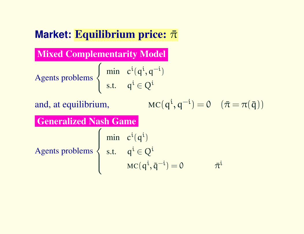
Market: Equilibrium price: π̄
Mixed Complementarity Model
Agents problems
min ci(qi,q−i)
s.t. qi ∈Qi
and, at equilibrium, MC(qi,q−i) = 0 (π̄= π(q̄))
Market: Equilibrium price: π̄
Mixed Complementarity Model
Agents problems
min ci(qi,q−i)
s.t. qi ∈Qi
and, at equilibrium, MC(qi,q−i) = 0 (π̄= π(q̄))
Generalized Nash Game
Agents problems
min ci(qi)
s.t. qi ∈Qi
MC(qi, q̃−i) = 0 (same π̄i for all)
Market: Equilibrium price: π̄
Mixed Complementarity Model
Agents problems
min ci(qi,q−i)
s.t. qi ∈Qi
and, at equilibrium, MC(qi,q−i) = 0 (π̄= π(q̄))
Generalized Nash Game
Agents problems
min ci(qi)
s.t. qi ∈Qi
MC(qi, q̃−i) = 0 (same π̄ for all i)
A Variational Equilibrium of the game is a Generalized NashEquilibrium satisfying π̄i = π̄
Both models give same equilibrium
Mixed Complementarity Model
Agents problems
min ci(qi,q−i)
s.t. qi ∈Qi
and, at equilibrium, MC(qi,q−i) = 0 (π̄= π(q̄))
Generalized Nash Game
Agents problems
min ci(qi)
s.t. qi ∈Qi
MC(qi, q̃−i) = 0 (same π̄ for all i)
J.P. Luna, C. Sagastizábal, M. Solodov. Complementarity and game-theoretical models for equilibria in energy markets:deterministic and risk-averse formulations. Ch. 10 in Risk Management in Energy Production and Trading, (R.Kovacevic, G. Pflüg and M. T. Vespucci), "Int. Series in Op. Research and Manag. Sci.", Springer, 2013.
Both models yield equivalent VIs
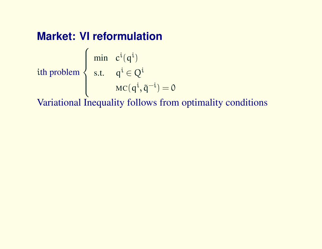
Market: VI reformulation
ith problem
min ci(qi)
s.t. qi ∈Qi
MC(qi, q̃−i) = 0
Variational Inequality follows from optimality conditions
Market: VI reformulation
ith problem
min ci(qi)
s.t. qi ∈Qi
MC(qi, q̃−i) = 0 (π̄)
Variational Inequality follows from optimality conditions
1st order OC
(primal form)⟨∇qic
i(q̄i),qi− q̄i⟩≥ 0
∀qi ∈Qi∩MC
Market: VI reformulation
ith problem
min ci(qi)
s.t. qi ∈Qi
MC(qi, q̃−i) = 0 (π̄i)
Variational Inequality follows from optimality conditions
1st order OC
(primal form)⟨∇qic
i(q̄i),qi− q̄i⟩≥ 0
∀qi ∈Qi∩MC
In VI(F,C) :⟨F(q̄),q− q̄
⟩≥ 0 ∀ feasible q
• the VI operator F(q) =N∏i=1
Fi(q) for Fi(q) = ∇qici(qi)
• the VI feasible set C=
N∏i=1
Qi⋂{
q : MC(q) = 0}
Market: VI reformulation
ith problem
min ci(qi)
s.t. qi ∈Qi
MC(qi, q̃−i) = 0 (π̄i)
Variational Inequality follows from optimality conditions
1st order OC
(primal form)⟨∇qic
i(q̄i),qi− q̄i⟩≥ 0
∀qi ∈Qi∩MC
In VI(F,C) :⟨F(q̄),q− q̄
⟩≥ 0 ∀ feasible q
• the VI operator F(q) =N∏i=1
Fi(q) for Fi(q) = ∇qici(qi)
• the VI feasible set C=
N∏i=1
Qi⋂{
q : MC(q) = 0}decomposability
NOTE: MC does not depend on i: constraint is shared
Incorporating a Capacity Market
Suppose producers pay Ii(zi)
to invest in an increase zi in production capacity
Production bounds go from 0≤ qi ≤ qimax (≡ qi ∈Qi)to 0≤ qi ≤ qimax+zi (zi,qi) ∈ Xi
Incorporating a Capacity Market
Suppose producers pay Ii(zi)
to invest in an increase zi in production capacity
Production bounds go from 0≤ qi ≤ qimax (≡ qi ∈Qi)to 0≤ qi ≤ qimax+zi (zi,qi) ∈ Xi
Incorporating a Capacity Market
Suppose producers pay Ii(zi)
to invest in an increase zi in production capacity
Production bounds go from 0≤ qi ≤ qimax (≡ qi ∈Qi)to 0≤ qi ≤ qimax+zi (zi,qi) ∈ Xi
ith problem
min Ii(zi)+ci(qi)
s.t. (zi,qi) ∈ Xi
MC(qi,q−i) = 0
≡minIi(zi)+V i(zi)
V i(zi) ={
minci(qi)
(zi,qi) ∈Xi
MC(qi,q−i) = 0
can this problem be rewritten as a 2-level problem?
Incorporating a Capacity Market
When trying to rewrite min Ii(zi)+V i(zi) using
V i(zi),q−i) =
minci(qi)
(zi,qi) ∈ Xi
MC(qi,q−i) = 0
a difficulty arises.
Incorporating a Capacity Market
When trying to rewrite min Ii(zi)+V i(zi) using
V i(zi, q−i ) =
minci(qi)
(zi,qi) ∈ Xi
MC(qi, q−i ) = 0
a difficulty arises.The function V i depends on (zi,q−i), the second-levelproblem is a Generalized Nash Game (hard!)
Incorporating a Capacity Market
When trying to rewrite min Ii(zi)+V i(zi) using
V i(zi,q−i) =
minci(qi)
(zi,qi) ∈ Xi
MC(qi,q−i) = 0
a difficulty arises.The function V i depends on (zi,q−i), the second-levelproblem is a Generalized Nash Game (hard!)Consistent with reality: Agents will keep competing aftercapacity expansion
Incorporating a Capacity Market
When trying to rewrite min Ii(zi)+V i(zi) using
V i(zi,q−i) =
minci(qi)
(zi,qi) ∈ Xi
MC(qi,q−i) = 0
a difficulty arises.The function V i depends on (zi,q−i), the second-levelproblem is a Generalized Nash Game (hard!)Consistent with reality: Agents will keep competing aftercapacity expansion. Similarly for Mixed Complementaritymodel
Incorporating a Capacity Market
When trying to rewrite min Ii(zi)+V i(zi) using
V i(zi,q−i) =
minci(qi)
(zi,qi) ∈ Xi
MC(qi,q−i) = 0
a difficulty arises.The function V i depends on (zi,q−i), the second-levelproblem is a Generalized Nash Game (hard!)Consistent with reality: Agents will keep competing aftercapacity expansion. Similarly for Mixed Complementaritymodel and 2 stage with recourse, even without expansion
Investment variables are (naturally) the same for all realizations: zi
Production variables are (naturally) different for each realization: qik
ith problem
for scenario k
min Ii(zi)+cik(qk)
s.t. (zi,qik) ∈ XikMCk(q
ik,q
−ik ) = 0
Two-stage formulation with recourse not possibleSingle-stage formulation instead: find a capacityexpansion compatible with K scenarios of competition(likewise for generation-only market)
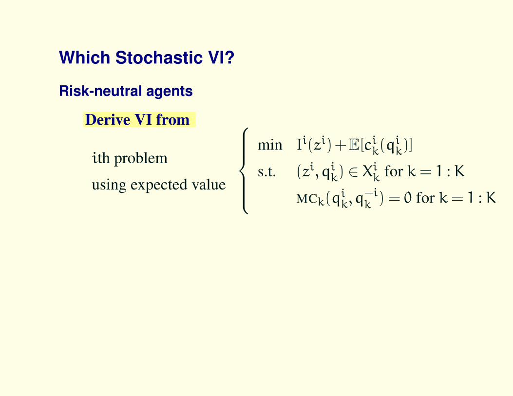
Which Stochastic VI?
Risk-neutral agents
Derive VI from
ith problem
using expected value
min Ii(zi)+E[cik(q
ik)]
s.t. (zi,qik) ∈ Xik for k= 1 : K
MCk(qik,q
−ik ) = 0 for k= 1 : K
Which Stochastic VI?
Risk-neutral agents
Derive VI from
ith problem
using expected value
min Ii(zi)+E[cik(q
ik)]
s.t. (zi,qik) ∈ Xik for k= 1 : K
MCk(qik,q
−ik ) = 0 for k= 1 : K
• a VI operator F involving ∇Ii(zi)×∇qi1:KE[ci1:K(q)
]• a VI feasible set C=
K∏k=1
N∏i=1
Xik⋂{
qk : MCk(qk) = 0}
Which Stochastic VI?
Risk-neutral agents
Derive VI from
ith problem
using expected value
min Ii(zi)+E[cik(q
ik)]
s.t. (zi,qik) ∈ Xik for k= 1 : K
MCk(qik,q
−ik ) = 0 for k= 1 : K
• a VI operator F involving ∇Ii(zi)×∇qi1:KE[ci1:K(q)
]• a VI feasible set C=
K∏k=1
N∏i=1
Xik⋂{
qk : MCk(qk) = 0}
decomposability
Which Stochastic VI?
Risk-neutral agents
Derive VI from
ith problem
using expected value
min Ii(zi)+E[cik(q
ik)]
s.t. (zi,qik) ∈ Xik for k= 1 : K
MCk(qik,q
−ik ) = 0 for k= 1 : K
• a VI operator F involving ∇Ii(zi)×∇qi1:KE[ci1:K(q)
]• a VI feasible set C=
K∏k=1
N∏i=1
Xik⋂{
qk : MCk(qk) = 0}
decomposabilitythere is no coupling between scenarios (E is linear)
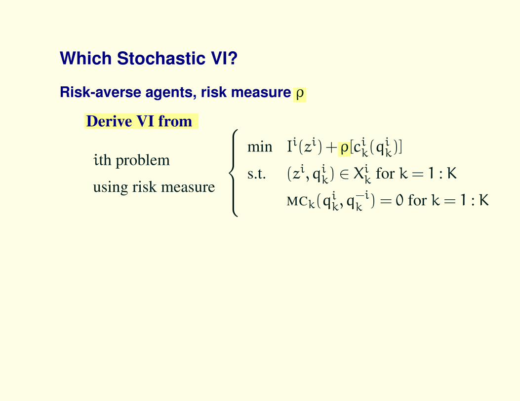
Which Stochastic VI?
Risk-averse agents, risk measure ρ
Derive VI from
ith problem
using risk measure
min Ii(zi)+ρ[cik(q
ik)]
s.t. (zi,qik) ∈ Xik for k= 1 : K
MCk(qik,q
−ik ) = 0 for k= 1 : K
Which Stochastic VI?
Risk-averse agents, risk measure ρ
Derive VI from
ith problem
using risk measure
min Ii(zi)+ρ[cik(q
ik)]
s.t. (zi,qik) ∈ Xik for k= 1 : K
MCk(qik,q
−ik ) = 0 for k= 1 : K
Difficulties arise: The risk measure is in general nonsmooth
ρ(Z) :=AV@R ε(Z) = minu{u+ 1
1−εE([Zk−u]+
)}: it is
a value-function and [·]+ is nonsmooth
• the VI operator F involves ∇Ii(zi)×∂qi1:Kρ[ci1:K(q)
],
multivalued
Two ways of handling multivalued VI operator
Reformulation:Introduce AV@R directly into the agent problem, byrewriting []+ in
ρ(Z) := minu
{u+
1
1−εE([Zk−u]+
)}by means of new variables and constraints
Two ways of handling multivalued VI operator
Reformulation:Introduce AV@R directly into the agent problem, byrewriting []+ in
ρ(Z) := minu
{u+
1
1−εE([Zk−u]+
)}by means of new variables and constraints
Smoothing:Smooth the [·]+-function and solve the smoothed VI
ρ`(Z) := minu
{u+
1
1−εE(σ` (Zk−u)
)},
for smoothing σ`→ [·]+ uniformly as `→∞
Reformulation ρ(Z) = minu{u+ 1
1−εE([Zk−u]+
)}
FROM
min Ii(zi)+ρ[cik(q
ik)]
s.t. (zi,qik) ∈ Xik for k= 1 : K
MCk(qik,q
−ik ) = 0 for k= 1 : K
TO:
min Ii(zi)+ui + 11−εE
(Ti
k
)s.t. (zi,qik) ∈ Xik for k= 1 : K
MCk(qik,q
−ik ) = 0 for k= 1 : K
T ik ≥ cik(qik)−ui ,T ik ≥ 0 for k= 1 : K,u ∈ IR
Reformulation ρ(Z) = minu{u+ 1
1−εE([Zk−u]+
)}
FROM
min Ii(zi)+ρ[cik(q
ik)]
s.t. (zi,qik) ∈ Xik for k= 1 : K
MCk(qik,q
−ik ) = 0 for k= 1 : K
TO:
min Ii(zi)+ui + 11−εE
(Ti
k
)s.t. (zi,qik) ∈ Xik for k= 1 : K
MCk(qik,q
−ik ) = 0 for k= 1 : K
T ik ≥ cik(qik)−ui ,T ik ≥ 0 for k= 1 : K,u ∈ IR
NOTE: new constraint is NOT shared: no longer ageneralized Nash game, but a bilinear CP (how to show ∃?).
Assessing both options
PATH can be used for the two variants.
+ Reformulation
eliminates nonsmoothness
Non-separable feasible set
+ Smoothing
To drive smoothing parameter to 0: repeated VI solves
Keeps feasible set separable by scenarios: easier VI
Assessing both options
PATH can be used for the two variants.
+ Reformulation
eliminates nonsmoothness
Non-separable feasible set
+ Smoothing
To drive smoothing parameter to 0: repeated VI solves
Keeps feasible set separable by scenarios: easier VI
Provides existence result!
Smoothing
We use smooth approximations ρ`
ρ`(Z) := minu
{u+
1
1−εE[σ`(Zk−u)
]},
for smoothing σ`→ [·]+ uniformly as `→∞. For instance,
σ`(t) = (t+√t2+4τ2` )/2
for τ`→ 0.
Since ρ` is smooth, VI(F`,C) has a a single-valued VI
operator involving ∇qiρ`[(cik(qk))
Kk=1
]
Theorems
• like AV@R, ρ` is a risk-measure
– convex, monotone, and translation equi-variant,
– but not positively homogeneous (only coherent in the limit).
• ρ` is C2 for strictly convex smoothings such as
σ`(t) = (t+√t2+4τ2` )/2
• Any accumulation point of the smoothed problems solvesthe original risk-averse (non-smooth) problem as `→∞.
: existence result!
Theorems
• like AV@R, ρ` is a risk-measure
– convex, monotone, and translation equi-variant,
– but not positively homogeneous (only coherent in the limit).
• ρ` is C2 for strictly convex smoothings such as
σ`(t) = (t+√t2+4τ2` )/2
• Any accumulation point of the smoothed problems solvesthe original risk-averse (non-smooth) problem as `→∞.
existence result!Reference: An approximation scheme for a class of risk-averse stochastic
equilibrium problems. Luna, Sagastizábal, Solodov
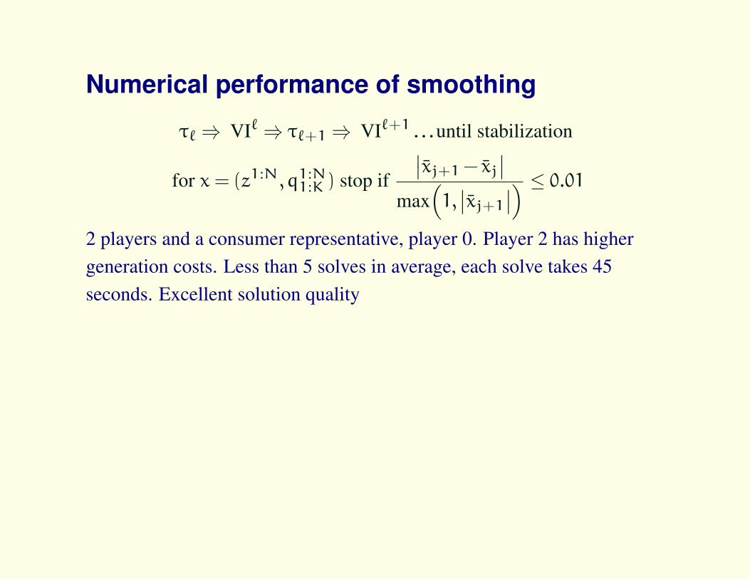
Numerical performance of smoothing
τ`⇒ VI`⇒ τ`+1⇒ VI`+1 . . .until stabilization
for x= (z1:N,q1:N1:K ) stop if
∣∣x̄j+1− x̄j∣∣max
(1,∣∣x̄j+1∣∣) ≤ 0.01
2 players and a consumer representative, player 0. Player 2 has highergeneration costs. Less than 5 solves in average, each solve takes 45seconds. Excellent solution quality
After the first VI, PATH solves much faster VIs for ` > 1
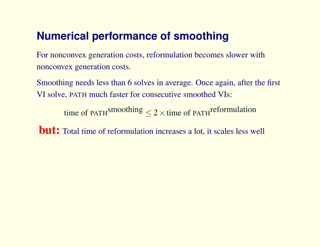
Numerical performance of smoothing
For nonconvex generation costs, reformulation becomes slower withnonconvex generation costs.
Smoothing needs less than 6 solves in average. Once again, after the firstVI solve, PATH much faster for consecutive smoothed VIs:
time of PATHsmoothing ≤ 2× time of PATHreformulation
but: Total time of reformulation increases a lot, it scales less well
Final Comments• When in the agents’ problems the objective or some constraint
depends on actions of other agents, writing down the stochasticgame/VI can be tricky (which selection mechanism in a 2-stage setting?)
• Handling nonsmoothness via reformulation seems inadequate forlarge instances
• Smoothing solves satisfactorily the original risk-averse nonsmoothproblem for moderate τ (no need to make τ→ 0)
• Smoothing preserves separability; it is possible to combine
– Benders’ techniques (along scenarios) with
– Dantzig-Wolfe decomposition (along agents)
• Decomposition matters: for European Natural Gas network– Solving VI directly with PATH solver S. Dirkse, M. C. Ferris, and T. Munson
– Using DW-decomposition saves 2/3 of solution time