Stochastic flows in the Brownian web and net Emmanuel Schertzer Rongfeng Sun Jan M. Swart May 28, 2013 Abstract It is known that certain one-dimensional nearest-neighbor random walks in i.i.d. random space-time environments have diffusive scaling limits. Here, in the continuum limit, the random environment is represented by a ‘stochastic flow of kernels’, which is a collection of random kernels that can be loosely interpreted as the transition probabilities of a Markov process in a random environment. The theory of stochastic flows of kernels was first developed by Le Jan and Raimond, who showed that each such flow is characterized by its n-point motions. Our work focuses on a class of stochastic flows of kernels with Brownian n-point motions which, after their inventors, will be called Howitt-Warren flows. Our main result gives a graphical construction of general Howitt-Warren flows, where the underlying random environment takes on the form of a suitably marked Brownian web. This extends earlier work of Howitt and Warren who showed that a special case, the so-called ‘erosion flow’, can be constructed from two coupled ‘sticky Brownian webs’. Our construction for general Howitt-Warren flows is based on a Poisson marking procedure developed by Newman, Ravishankar and Schertzer for the Brownian web. Alternatively, we show that a special subclass of the Howitt-Warren flows can be constructed as random flows of mass in a Brownian net, introduced by Sun and Swart. Using these constructions, we prove some new results for the Howitt-Warren flows. In particular, we show that the kernels spread with a finite speed and have a locally finite support at deterministic times if and only if the flow is embeddable in a Brownian net. We show that the kernels are always purely atomic at deterministic times, but, with the exception of the erosion flows, exhibit random times when the kernels are purely non- atomic. We moreover prove ergodic statements for a class of measure-valued processes induced by the Howitt-Warren flows. Our work also yields some new results in the theory of the Brownian web and net. In particular, we prove several new results about coupled sticky Brownian webs and about a natural coupling of a Brownian web with a Brownian net. We also introduce a ‘finite graph representation’ which gives a precise description of how paths in the Brownian net move between deterministic times. MSC 2010. Primary: 82C21 ; Secondary: 60K35, 60K37, 60D05. Keywords. Brownian web, Brownian net, stochastic flow of kernels, measure-valued process, Howitt-Warren flow, linear system, random walk in random environment, finite graph repre- sentation. Acknowledgement. R. Sun is supported by grants R-146-000-119-133 and R-146-000-148- 112 from the National University of Singapore. J.M. Swart is sponsored by GA ˇ CR grants 201/07/0237 and 201/09/1931. Contents 1 Introduction 3 1.1 Overview ............................................ 3 1.2 Discrete Howitt-Warren flows ................................. 4 1.3 Scaling limits of discrete Howitt-Warren flows ........................ 6 1.4 Outline and discussion ..................................... 10 2 Results for Howitt-Warren flows 10 2.1 Stochastic flows of kernels ................................... 10 2.2 Howitt-Warren flows ...................................... 12 2.3 Path properties ......................................... 14 2.4 Infinite starting measures and discrete approximation ................... 18 2.5 Ergodic properties ....................................... 19 1
Transcript
Stochastic flows in the Brownian web and net
Emmanuel Schertzer Rongfeng Sun Jan M. Swart
May 28, 2013
AbstractIt is known that certain one-dimensional nearest-neighbor random walks in i.i.d. randomspace-time environments have diffusive scaling limits. Here, in the continuum limit, therandom environment is represented by a ‘stochastic flow of kernels’, which is a collection ofrandom kernels that can be loosely interpreted as the transition probabilities of a Markovprocess in a random environment. The theory of stochastic flows of kernels was firstdeveloped by Le Jan and Raimond, who showed that each such flow is characterized by itsn-point motions. Our work focuses on a class of stochastic flows of kernels with Browniann-point motions which, after their inventors, will be called Howitt-Warren flows.
Our main result gives a graphical construction of general Howitt-Warren flows, wherethe underlying random environment takes on the form of a suitably marked Brownianweb. This extends earlier work of Howitt and Warren who showed that a special case, theso-called ‘erosion flow’, can be constructed from two coupled ‘sticky Brownian webs’. Ourconstruction for general Howitt-Warren flows is based on a Poisson marking proceduredeveloped by Newman, Ravishankar and Schertzer for the Brownian web. Alternatively,we show that a special subclass of the Howitt-Warren flows can be constructed as randomflows of mass in a Brownian net, introduced by Sun and Swart.
Using these constructions, we prove some new results for the Howitt-Warren flows. Inparticular, we show that the kernels spread with a finite speed and have a locally finitesupport at deterministic times if and only if the flow is embeddable in a Brownian net.We show that the kernels are always purely atomic at deterministic times, but, with theexception of the erosion flows, exhibit random times when the kernels are purely non-atomic. We moreover prove ergodic statements for a class of measure-valued processesinduced by the Howitt-Warren flows.
Our work also yields some new results in the theory of the Brownian web and net. Inparticular, we prove several new results about coupled sticky Brownian webs and abouta natural coupling of a Brownian web with a Brownian net. We also introduce a ‘finitegraph representation’ which gives a precise description of how paths in the Brownian netmove between deterministic times.
MSC 2010. Primary: 82C21 ; Secondary: 60K35, 60K37, 60D05.Keywords. Brownian web, Brownian net, stochastic flow of kernels, measure-valued process,Howitt-Warren flow, linear system, random walk in random environment, finite graph repre-sentation.Acknowledgement. R. Sun is supported by grants R-146-000-119-133 and R-146-000-148-112 from the National University of Singapore. J.M. Swart is sponsored by GACR grants201/07/0237 and 201/09/1931.
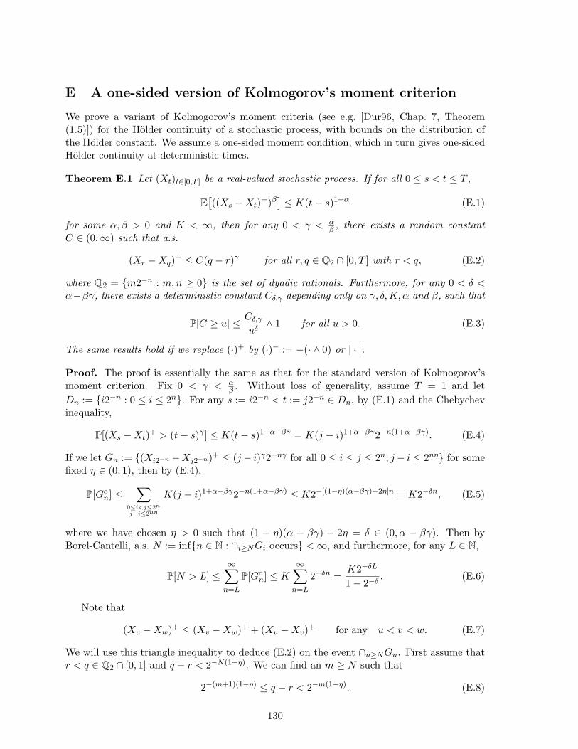
E A one-sided version of Kolmogorov’s moment criterion 130
2
1 Introduction
1.1 Overview
In [LR04a], Le Jan and Raimond introduced the notion of a stochastic flow of kernels, whichis a collection of random probability kernels that can be loosely viewed as the transitionkernels of a Markov process in a random space-time environment, where restrictions of theenvironment to disjoint time intervals are independent and the environment is stationaryin time. For suitable versions of such a stochastic flow of kernels (when they exist), thisloose interpretation is exact, see Definition 2.1 below and the remark following it. Given theenvironment, one can sample n independent copies of the Markov process and then averageover the environment. This defines the n-point motion for the flow, which satisfies a naturalconsistency condition: namely, the marginal distribution of any k components of an n-pointmotion is necessarily a k-point motion. A fundamental result of Le Jan and Raimond [LR04a]shows that conversely, any family of Feller processes that is consistent in this way gives riseto an (essentially) unique stochastic flow of kernels.
As an example, in [LR04b], the authors used Dirichlet forms to construct a consistentfamily of reversible n-point motions on the circle, which are α-stable Levy processes with someform of sticky interaction characterized by a real parameter θ. In particular, for α = 2, theseare sticky Brownian motions. Subsequently, Howitt and Warren [HW09a] used a martingaleproblem approach to construct a much larger class of consistent Feller processes on R, whichare Brownian motions with some form of sticky interaction characterized by a finite measure νon [0, 1]. In particular, if ν is a multiple of the Lebesgue measure, these are the sticky Brownianmotions of Le Jan and Raimond. From now on, and throughout this paper, we specialize to thecase of Browian underlying motions. By the general result of Le Jan and Raimond mentionedabove, the sticky Brownian motions of Le Jan and Raimond, resp. Howitt and Warren, are then-point motions of an (essentially) unique stochastic flow of kernels on R, which we call a LeJan-Raimond flow, resp. Howitt-Warren flow (the former being a special case of the latter).It has been shown in [LL04, HW09a] that these objects can be obtained as diffusive scalinglimits of one-dimensional random walks in i.i.d. random space-time environments.
The main goal of the present paper is to give a graphical construction of Howitt-Warrenflows that follows as closely as possible the discrete construction of random walks in an i.i.d.random environment. In particular, we want to make explicit what represents the randomenvironment in the continuum setting. The original construction of Howitt-Warren flows usingn-point motions does not tell us much about this. In [HW09b], it was shown that the Howitt-Warren flow with ν = δ0 +δ1, known as the erosion flow, can be constructed using two coupledBrownian webs, where one Brownian web serves as the random space-time environment, whilethe conditional law of the second Brownian web determines the stochastic flow of kernels.
We will extend this construction to general Howitt-Warren flows, where in the generalcase, the random environment consists of a Brownian web together with a marked Poissonpoint process which is concentrated on the so-called points of type (1, 2) of the Brownianweb. A central tool in this construction is a Poisson marking procedure invented by Newman,Ravishankar and Schertzer in [NRS10]. Of course, we also make extensive use of the theoryof the Brownian web developed in [TW98, FINR04]. For a special subclass of the Howitt-Warren flows, we will show that alternatively the random space-time environment can berepresented as a Brownian net, plus a countable collection of i.i.d. marks attached to its so-called separation points. Here, we use the theory of the Brownian net, which was developed
3
in [SS08] and [SSS09].Using our graphical construction, we prove a number of new properties for the Howitt-
Warren flows. In particular, we give necessary and sufficient conditions in terms of the measureν for the random kernels to spread with finite speed, for their support to consist of isolatedpoints at deterministic times, and for the existence of random times when the kernels are non-atomic (Theorems 2.5, 2.7 and 2.8 below). We moreover use our construction to prove theexistence of versions of Howitt-Warren flows with nice regularity properties (Proposition 3.8below), in particular, versions which can be interpreted as bona fide transition kernels ina random space-time environment. Lastly, we study the invariant laws for measure-valuedprocesses associated with the Howitt-Warren flows (Theorem 2.11).
Our graphical construction of the Howitt-Warren flows is to a large extent motivated by itsdiscrete space-time counterpart, i.e., random walks in i.i.d. random space-time environmentson Z. Many of our proofs will also be based on discrete approximation. Therefore, in therest of the introduction, we will introduce a class of random walks in i.i.d. random space-time environments and some related objects of interest, and sketch heuristically how theBrownian web and the Brownian net will arise in the representation of the random space-timeenvironment for the Howitt-Warren flows. An outline of the rest of the paper will be given atthe end of the introduction.
Incidentally, we note that random walks in i.i.d. random space-time environments havebeen used in the physics literature to model the flow of stress in a granular medium, calledthe q model, see e.g. [LMY01, JM11] and the references therein. The Howitt-Warren flows weconsider are effectively scaling limits of so-called near-critical q models.
1.2 Discrete Howitt-Warren flows
Let Z2even := (x, t) : x, t ∈ Z, x + t is even be the even sublattice of Z2. We interpret the
first coordinate x as space and the second coordinate t as time, which is plotted vertically infigures. Let ω := (ωz)z∈Z2
evenbe i.i.d. [0, 1]-valued random variables with common distribution
µ. We view ω as a random space-time environment for a random walk, such that conditionalon the environment ω, if the random walk is at time t at the position x, then in the next unittime step the walk jumps to x + 1 with probability ω(x,t) and to x − 1 with the remainingprobability 1− ω(x,t) (see Figure 1).
To formalize this, let P denote the law of the environment ω and for each (x, s) ∈ Z2even,
let Qω(x,s) denote the conditional law, given the random environment ω, of the random walk
in random environment X = (X(t))t≥s we have just described, started at time s at positionX(s) = x. Since parts of the random environment belonging to different times are independent,it is not hard to see that under the averaged (or ‘annealed’) law
∫P(dω)Qω
(x,s), the process Xis still a Markov chain, which in each time step jumps to the right with probability
∫µ(dq)q
and to the left with the remaining probability∫µ(dq)(1− q). Note that this is quite different
from the usual random walk in random environment (RWRE) where the randomness is fixedfor all time, and the averaged motion no longer has the Markov property.
We will be interested in three objects associated with the random walks in the i.i.d. ran-dom space-time environment ω, namely: random transition kernels, n-point motions, and ameasure-valued process. The law of each of these objects is uniquely characterized by µ and,conversely, uniquely determines µ.
First of all, the random environment ω determines a family of random transition probability
4
(x, t)
0.96 1 1 0.81
0.74 0.01 0 0.99
0.68 0.56 0.01 0
0 0 0.58
0.94 ω(x,t) 0.95 0.85
1
0.99
0.86
0.93
0.02
0.99
Figure 1: Random walk on Z2even in a random environment ω.
kernels,Kωs,t(x, y) := Qω
(x,s)
[X(t) = y
] (s ≤ t, (x, s), (y, t) ∈ Z2
even
), (1.1)
which satisfy
(i)∑
y: (y,t)∈Z2even
Kωs,t(x, y)Kω
t,u(y, z) = Kωs,u(x, z)
(s ≤ t ≤ u, (x, s), (z, u) ∈ Z2
even).
(ii) For each t0 < · · · < tn, the random variables (Kωti−1,ti)i=1,...,n are independent.
(iii) Kωs,t and Kω
s+u,t+u are equal in law for each u ∈ Zeven := 2x : x ∈ Z.
We call the collection of random probability kernels (Kωs,t)s≤t the discrete Howitt-Warren flow
with characteristic measure µ. Such a collection is a discrete time analogue of a stochasticflow of kernels as introduced by Le Jan and Raimond in [LR04a] (see Definition 2.1 below).
Next, given the environment ω, we can sample a collection of independent random walks
( ~X(t))t≥0 =(X1(t), . . . , Xn(t)
)t≥0
(1.2)
in the random environment ω, started at time zero from deterministic sites x1, . . . , xn ∈ Zeven,respectively. It is easy to see that under the averaged law∫
P(dω)n⊗i=1
Qω(xi,0), (1.3)
the process ~X = ( ~X(t))t≥0 is still a Markov chain, which we call the discrete n-point motion.Its transition probabilities are given by
P(n)s,t (~x, ~y) =
∫P(dω)
n∏i=1
Kωs,t(xi, yi)
(s ≤ t, (xi, s), (yi, t) ∈ Z2
even, i = 1, . . . , n). (1.4)
5
Note that these discrete n-point motions are consistent in the sense that any k coordinates of~X are distributed as a discrete k-point motion. Each coordinate Xi is distributed as a nearest-neighbor random walk thats makes jumps to the right with probability
∫µ(dq)q. Because of
the spatial independence of the random environment, the coordinates evolve independentlywhen they are at different positions. To see that there is some nontrivial interaction whenthey are at the same position, note that if k + l coordinates are at position x at time t, thenthe probability that in the next time step the first k coordinates jump to x + 1 while thelast l coordinates jump to x − 1 equals
∫µ(dq)qk(1 − q)l, which in general does not factor
into (∫µ(dq)q)k(
∫µ(dq)(1 − q))l. Note that the law of ω(0,0) is uniquely determined by its
moments, which are in turn determined by the transition probabilities of the discrete n-pointmotions (for each n).
Finally, based on the family of kernels (Kωs,t)s≤t, we can define a measure-valued process
ρt(x) =∑
y∈Zeven
ρ0(y)Kω0,t(y, x)
(t ≥ 0, (x, t) ∈ Z2
even
), (1.5)
where ρ0 is any locally finite initial measure on Zeven. Note that conditional on ω, the processρ = (ρt)t≥0 evolves deterministically, with
Under the law P, the process ρ is a Markov chain, taking values alternatively in the spaces offinite measures on Zeven and Zodd := 2x + 1 : x ∈ Z. Note that (1.6) says that in the timestep from t to t+ 1, an ω(x,t)-fraction of the mass at x is sent to x+ 1 and the rest is sent tox− 1. Obviously, this dynamics preserves the total mass. In particular, if ρ0 is a probabilitymeasure, then ρt is a probability measure for all t ≥ 0. We call ρ the discrete Howitt-Warrenprocess.
We will be interested in the diffusive scaling limits of all these objects, which will be(continuum) Howitt-Warren flows and their associated n-point motions and measure-valuedprocesses, respectively. Note that the discrete Howitt-Warren flow (Kω
s,t)s≤t determines therandom environment ω a.s. uniquely. The law of (Kω
s,t)s≤t is uniquely determined by eitherthe law of its n-point motions or the law of its associated measure-valued process.
1.3 Scaling limits of discrete Howitt-Warren flows
We now recall from [HW09a] the conditions under which the n-point motions of a sequenceof discrete Howitt-Warren flows converge to the n-point motions of a (continuum) stochasticflow of kernels, which we call a Howitt-Warren flow. We will then use discrete approximationto sketch heuristically how such a Howitt-Warren flow can be constructed from a Brownianweb or net.
Let (εk)k∈N be positive constants tending to zero, and let (µk)k∈N be probability laws on[0, 1] satisfying1
(i) ε−1k
∫(2q − 1)µk(dq) −→
k→∞β,
(ii) ε−1k q(1− q)µk(dq) =⇒
k→∞ν(dq)
(1.7)
1We follow [HW09a] in our definition of ν. Many of our formulas, however, such as (2.3), (2.11) or (3.16)are more easily expressed in terms of 2ν than in ν. Loosely speaking, the reason for this is that in (1.7) (ii), theweight function q(1− q) arises from the fact that if α1, α2 are independent −1,+1-valued random variableswith P[αi = +1] = q (i = 1, 2), then P[α1 6= α2] = 2q(1− q).
6
for some β ∈ R and finite measure ν on [0, 1], where ⇒ denotes weak convergence. Howittand Warren [HW09a]2 proved that under condition (1.7), if we scale space by εk and time byε2k, then the discrete n-point motions with characteristic measure µk converge to a collection
of Brownian motions with drift β and some form of sticky interaction characterized by themeasure ν. These Brownian motions form a consistent family of Feller processes, hence by thegeneral result of Le Jan and Raimond mentioned in Section 1.1, they are the n-point motionsof some stochastic flow of kernels, which we call the Howitt-Warren flow with drift β andcharacteristic measure ν. The definition of Howitt-Warren flows and their n-point motionswill be given more precisely in Section 2.
Now let us use discrete approximation to explain heuristically how to construct a Howitt-Warren flow based on a Brownian web or net. The construction based on the Brownian netis conceptually easier, so we consider this case first.
Let β ∈ R and let ν be a finite measure on [0, 1]. Assuming, as we must in this case, that∫ ν(dq)q(1−q) <∞, we may define a sequence of probability measures µk on [0, 1] by
µk := bεkν + 12(1− (b+ c)εk)δ0 + 1
2(1− (b− c)εk)δ1
where b :=∫
ν(dq)q(1− q)
, c := β −∫
(2q − 1)ν(dq)q(1− q)
, ν(dq) :=ν(dq)
bq(1− q).
(1.8)
Then µk is a probability measure on [0, 1] for k sufficiently large (such that 1−(b+ |c|)εk ≥ 0),and the µk satisfy (1.7). Thus, when space is rescaled by εk and time by ε2
k, the discreteHowitt-Warren flow with characteristic measure µk approximates a Howitt-Warren flow withdrift β and characteristic measure ν.
Let ω〈k〉 := (ω〈k〉z )z∈Z2even
be i.i.d. with common law µk, which serves as the random environ-ment for a discrete Howitt-Warren flow with characteristic measure µk. We observe that forlarge k, most of the ω〈k〉z are either zero or one. In view of this, it is convenient to alternativelyencode ω〈k〉 as follows. For each z = (x, t) ∈ Z2
even, if ω〈k〉z ∈ (0, 1), then we call z a separationpoint, set ω〈k〉z = ω
〈k〉z , and we draw two arrows from z, leading respectively to (x ± 1, t + 1).
When ω〈k〉z = 0, resp. 1, we draw a single arrow from z to (x−1, t+1), resp. (x+1, t+1). Notethat the collection of arrows N 〈k〉 generates a branching-coalescing structure, called discretenet, on Z2
even (see Figure 2) and conditional on N 〈k〉, the ω〈k〉z at separation points z of N 〈k〉 areindependent with common law ν. Therefore the random environment ω〈k〉 can be representedby the pair (N 〈k〉, ω〈k〉), where a walk in such an environment must navigate along N 〈k〉, andwhen it encounters a separation point z, it jumps either left or right with probability 1− ω〈k〉,resp. ω〈k〉.
It turns out that the pair (N 〈k〉, ω〈k〉) has a meaningful diffusive scaling limit. In particular,if space is scaled by εk and time by ε2
k, then N 〈k〉 converges to a limiting branching-coalescingstructure N called the Brownian net, the theory of which was developed in [SS08, SSS09]. Inparticular, the separation points of N 〈k〉 have a continuum analogue, the so-called separationpoints of N , where incoming trajectories can continue along two groups of outgoing trajecto-ries. These separation points are dense in space and time, but countable. Conditional on N ,we can then assign i.i.d. random variables ωz with common law ν to the separation points ofN . The pair (N , ω) provides a representation for the random space-time environment under-lying the Howitt-Warren flow with drift β and characteristic measure ν. A random motion in
2Actually, the paper [HW09a] considers a continuous-time analogue of the discrete n-point motions definedin Section 1.2, but their proof, with minor modifications, also works in the discrete time setting. In Appendix Awe present a similar, but somewhat simplified convergence proof.
7
such a random environment must navigate along N , and whenever it comes to a separationpoint z, with probability 1 − ωz resp. ωz, it continues along the left resp. right of the twogroups of outgoing trajectories in N at z. We will recall the formal definition of the Browniannet and give a rigorous construction of a random motion navigating in N in Section 4.
0.96
0.86 0.56
ω(x,t)
(x, t)
Figure 2: Representation of the random environment (ω〈k〉z )z∈Z2even
in terms of a marked discretenet (N 〈k〉, ω〈k〉).
(x, t)
0.96 1 1 0.81
0.74 0.01 0 0.99
0.68 0.56 0.01 0
0 0 0.58
0.94 0.95 0.85
1
0.99
0.93
0.02
0.99
0.86
ω(x,t)
Figure 3: Representation of the random environment (ω〈k〉z )z∈Z2even
in terms of a marked discrete
web (W 〈k〉0 , ω〈k〉).
We now consider Howitt-Warren flows whose characteristic measure is a general finitemeasure ν. Let (µk)k∈N satisfy (1.7) and let ω〈k〉 := (ω〈k〉z )z∈Z2
evenbe an i.i.d. random space-
8
time environment with common law µk. Contrary to the previous situation, it will now ingeneral not be true that the most of the ω〈k〉z ’s are either zero or one. Nevertheless, it is stilltrue that for large k, most of the ω〈k〉z ’s are either close to zero or to one. To take advantageof this fact, conditional on ω〈k〉, we sample independent −1,+1-valued random variables(α〈k〉z )z∈Z2
evensuch that α〈k〉z = +1 with probability ω〈k〉z . For each z = (x, t) ∈ Z2
even, we draw
an arrow from (x, t) to (x+ α〈k〉z , t+1). These arrows define a coalescing structure W 〈k〉0 , calleddiscrete web, on Z2
even (see Figure 3). Think of these arrows as assigning to each point z apreferred direction, which, in most cases, will be +1 if ω〈k〉z is close to one and −1 if ω〈k〉z isclose to zero.
Now let us describe the joint law of (ω〈k〉, α〈k〉) differently. First of all, if we forget aboutω〈k〉, then the (α〈k〉z )z∈Z2
evenare just i.i.d. −1,+1-valued random variables which take the
value +1 with probability∫qµk(dq). Second, conditional on α〈k〉, the random variables
(ω〈k〉z )z∈Z2even
are independent with distribution
µlk :=
(1− q)µk(dq)∫(1− q)µk(dq)
, resp. µrk :=
qµk(dq)∫qµk(dq)
(1.9)
depending on whether α〈k〉z = −1 resp. +1. Therefore, we can alternatively construct ourrandom space-time environment ω〈k〉 in such a way, that first we construct an i.i.d. collectionα〈k〉 as above, and then conditional on α〈k〉, independently for each z ∈ Z2
even, we choose ω〈k〉zwith law µl
k if α〈k〉z = −1 and law µrk if α〈k〉z = +1.
Let W 〈k〉0 denote the coalescing structure on Z2even generated by the arrows associated
with (α〈k〉z )z∈Z2even
(see Figure 3). Then (W 〈k〉0 , ω〈k〉) gives an alternative representation of therandom environment ω〈k〉. A random walk in such an environment navigates in such a waythat whenever it comes to a point z ∈ Z2
even, the walk jumps to the right with probabilityω〈k〉z and to the left with the remaining probability. The important thing to observe is that
if k is large, then ω〈k〉z is with large probability close to zero if α〈k〉 = −1 and close to one
if α〈k〉 = +1. In view of this, the random walk in the random environment (W 〈k〉0 , ω〈k〉) willmost of its time walk along paths in W
〈k〉0 .
It turns out that (W 〈k〉0 , ω〈k〉) has a meaningful diffusive scaling limit. In particular, ifspace is scaled by εk and time by ε2
k, then the coalescing structure W 〈k〉0 converges to a limitW0 called the Brownian web (with drift β), which loosely speaking is a collection of coalescingBrownian motions starting from every point in space and time. These provide the defaultpaths a motion in the limiting random environment must follow. The i.i.d. random variablesω〈k〉z turn out to converge to a marked Poisson point process which is concentrated on so-
called points of type (1, 2) in W0, which are points where there is one incoming path and twooutgoing paths. These points are divided into points of type (1, 2)l and (1, 2)r, dependingon whether the incoming path continues on the left or right. A random motion in such anenvironment follows paths in W0 by default, but whenever it comes to a marked point z oftype (1, 2), it continues along the left resp. right outgoing path with probability 1− ωz resp.ωz.3 We will give the rigorous construction in Section 3. The procedure of marking a Poisson
3In fact, this is not the full story, but describes only what happens if the measure ν from (1.7) is concentratedon (0, 1). If ν puts mass on the boundary of [0, 1], then a random motion in W0 will in addition, with a certainPoisson rate, decide to follow the non-default outgoing path at some unmarked points of type (1, 2). Inparticular, this is the only mechanism if ν is concentrated on 0, 1, i.e., for so-called erosion flows.
9
set of points of type (1, 2) that we need here was first developed by Newman, Ravishankar andSchertzer in [NRS10], who used it (among other things) to give an alternative construction ofthe Brownian net.
1.4 Outline and discussion
The rest of the paper is organized as follows. Sections 2–4 provide an extended introductionwhere we rigorously state our results. In Section 2, we recall the notion of a stochastic flowof kernels, first introduced in [LR04a], and Howitt and Warren’s [HW09a] sticky Brownianmotions, to give a rigorous definition of Howitt-Warren flows. We then state out main re-sults for these Howitt-Warren flows, including properties for the kernels and results for theassociated measure-valued processes. In Sections 3 and 4 we make the heuristics from Sec-tion 1.3 rigorous. In Section 3, in particular in Theorem 3.7, we present our construction ofHowitt-Warren flows based on a ‘reference’ Brownian web with a Poisson marking, which isthe main result of this paper. Along the way, we will recall the necessary background on theBrownian web. In Section 4, we show that a special subclass of the Howitt-Warren flows canbe constructed alternatively as flows of mass in the Brownian net. Along the way, we willrecall the necessary background on the Brownian net and establish some new results on acoupling between a Brownian web and a Brownian net. Sections 5–10 are devoted to proofs.In particular, we refer to Section 5 for an outline of the proofs. The paper concludes with anumber of appendices and a list of notation.
Our work leaves several open problems. One question, for example, is how to characterizethe measure-valued processes associated with a Howitt-Warren flow (see (2.1) below) by meansof a well-posed martingale problem. Other questions (martingale problem formulation, pathproperties) refer to the duals (in the sense of linear systems duality) of these measure-valuedprocesses, introduced in (11.1) below, which we have not investigated in much detail.
Moving away from the Brownian case, we note that it is an open problem whether ourmethods can be generalized to other stochastic flows of kernels than those introduced byHowitt and Warren. In particular, this applies to the stochastic flows of kernels with α-stableLevy n-point motions introduced in [LR04b] for 1 < α < 2. A first step on this road wouldbe the construction of an α-stable Levy web which should generalize the presently knownBrownian web. Some first steps in this direction have recently been taken in [EMS13].
2 Results for Howitt-Warren flows
In this section, we recall the notion of a stochastic flow of kernels, define the Howitt-Warrenflows, and state our results on these Howitt-Warren flows, which include almost sure pathproperties and ergodic theorems for the associated measure-valued processes. The proofs ofthese results are based on our graphical construction of the Howitt-Warren flows, which wepostpone to Sections 3–4 due to the extensive background we need to recall.
2.1 Stochastic flows of kernels
In [LR04a], Le Jan and Raimond developed a theory of stochastic flows of kernels, whichmay admit versions that can be interpreted as the random transition probability kernels of aMarkov process in a stationary random space-time environment. The notion of a stochasticflow of kernels generalizes the usual notion of a stochastic flow, which is a family of random
10
mappings (φωs,t)s≤t from a space E to itself. In the special case that all kernels are delta-measures, a stochastic flow of kernels reduces to a stochastic flow in the usual sense of theword.
Since stochastic flows of kernels play a central role in our work, we take some time torecall their defintion. For any Polish space E, we let B(E) denote the Borel σ-field on Eand writeM(E) andM1(E) for the spaces of finite measures and probability measures on E,respectively, equipped with the topology of weak convergence and the associated Borel σ-field.By definition, a probability kernel on E is a function K : E × B(E) → R such that the mapx 7→ K(x, · ) from E to M1(E) is measurable. By a random probability kernel, defined onsome probability space (Ω,F ,P), we will mean a function K : Ω × E × B(E) → R such thatthe map (ω, x) 7→ Kω(x, · ) from Ω × E to M1(E) is measurable. We say that two randomprobability kernelsK,K ′ are equal in finite dimensional distributions if for each x1, . . . , xn ∈ E,the n-tuple of random probability measures
(K(x1, · ), . . . ,K(xn, · )
)is equally distributed
with(K ′(x1, · ), . . . ,K ′(xn, · )
). We say that two or more random probability kernels are
independent if their finite-dimensional distributions are independent.
Definition 2.1 (Stochastic flow of kernels) A stochastic flow of kernels on E is a col-lection (Ks,t)s≤t of random probability kernels on E such that 4
(i) For all s ≤ t ≤ u and x ∈ E, a.s. Ks,s(x,A) = δx(A) and∫EKs,t(x,dy)Kt,u(y,A) =
Ks,u(x,A) for all A ∈ B(E).
(ii) For each t0 < · · · < tn, the random probability kernels (Kti−1,ti)i=1,...,n are independent.
(iii) Ks,t and Ks+u,t+u are equal in finite-dimensional distributions for each real s ≤ t and u.
The finite-dimensional distributions of a stochastic flow of kernels are the laws of n-tuples ofrandom probability measures of the form
(Ks1,t1(x1, · ), . . . ,Ksn,tn(xn, · )
), where xi ∈ E and
si ≤ ti, i = 1, . . . , n.
Remark. If the random set of probability 1 on which Definition 2.1 (i) holds can be chosenuniformly for all s ≤ t ≤ u and x ∈ E, then we can interpret (Ks,t)s≤t as bona fide transitionkernels of a random motion in random environment. For the stochastic flows of kernels weare interested in, we will prove the existence of a version of K which satisfies this property(see Proposition 2.3 below). To the best of our knowledge, it is not known whether such aversion always exists for general stochastic flows of kernels, even if we restrict ourselves tothose defined by a consistent family of Feller processes.
If (Ks,t)s≤t is a stochastic flow of kernels and ρ0 is a finite measure on E, then setting
ρt(dy) :=∫ρ0(dx)K0,t(x,dy) (t ≥ 0) (2.1)
defines an M(E)-valued Markov process (ρt)t≥0. Moreover, setting
P(n)t−s(~x, d~y) := E
[Ks,t(x1,dy1) · · ·Ks,t(xn,dyn)
](~x ∈ En, s ≤ t) (2.2)
4For simplicity, we have omitted two regularity conditions on (Ks,t)s≤t from the original definition in [LR04a,Def. 2.3], which are some form of weak continuity of Ks,t(x, ·) in x, s and t. It is shown in that paper thata stochastic flow of kernels on a compact metric space E satisfies these regularity conditions if and only if itarises from a consistent family of Feller processes.
11
defines a Markov transition function on En. We call the Markov process with these transitionprobabilities the n-point motion associated with the stochastic flow of kernels (Ks,t)s≤t. Weobserve that the n-point motions of a stochastic flow of kernels satisfy a natural consistencycondition: namely, the marginal distribution of any k components of an n-point motion isnecessarily a k-point motion for the flow. A fundamental result of Le Jan and Raimond[LR04a, Thm 2.1] states that conversely, any consistent family of Feller processes on a locallycompact space E gives rise to a stochastic flow of kernels on E which is unique in finite-dimensional distributions.5
2.2 Howitt-Warren flows
As will be proved in Proposition A.5 below, under the condition (1.7), if space and timeare rescaled respectively by εk and ε2
k, then the n-point motions associated with the discreteHowitt-Warren flow introduced in Section 1.2 with characteristic measure µk converge to acollection of Brownian motions with drift β and some form of sticky interaction characterizedby the measure ν. These Brownian motions solve a well-posed martingale problem, which weformulate now.
Let β ∈ R, ν a finite measure on [0, 1], and define constants (β+(m))m≥1 by
β+(1) :=β and
β+(m) :=β + 2∫ν(dq)
m−2∑k=0
(1− q)k (m ≥ 2).(2.3)
We note that in terms of these constants, (1.7) is equivalent to
ε−1k
∫ (1− 2(1− q)m
)µk(dq) −→
k→∞β+(m) (m ≥ 1). (2.4)
For ∅ 6= ∆ ⊂ 1, . . . , n, we define
f∆(~x) := maxi∈∆
xi and g∆(~x) :=∣∣i ∈ ∆ : xi = f∆(~x)
∣∣ (~x ∈ Rn), (2.5)
where | · | denotes the cardinality of a set.The martingale problem we are about to formulate was invented by Howitt and Warren
[HW09a]. We have reformulated their definition in terms of the functions f∆ in (2.5), whichform a basis of the vector space of test functions used in [HW09a, Def 2.1] (see Appendix A fora proof). This greatly simplifies the statement of the martingale problem and also facilitatesour proof of the convergence of the n-point motions of discrete Howitt-Warren flows.
Definition 2.2 (Howitt-Warren martingale problem) We say that an Rn-valued process~X = ( ~X(t))t≥0 solves the Howitt-Warren martingale problem with drift β and characteristicmeasure ν if ~X is a continuous, square-integrable semimartingale, the covariance process be-tween Xi and Xj is given by
5In fact, [LR04a, Thm 2.1] is stated only for compact metrizable spaces, but the extension to locally compactE is straightforward using the one-point compactification of E.
12
and, for each nonempty ∆ ⊂ 1, . . . , n,
f∆
(~X(t)
)−∫ t
0β+
(g∆( ~X(s))
)ds (2.7)
is a martingale with respect to the filtration generated by ~X.
Remark. We could have stated a similar martingale problem where instead of the functionsf∆ from (2.5) we use the functions f∆(x) := mini∈∆ xi and we replace the β+(m) defined in(2.3) by
β−(1) := β and β−(m) := β − 2∫ν(dq)
m−2∑k=0
qk (m ≥ 2). (2.8)
It is not hard to prove that both martingale problems are equivalent.
Remark. When n = 2, condition (2.7) is equivalent to the condition that
X1(t)− βt, X2(t)− βt, |X1(t)−X2(t)| − 4ν([0, 1])∫ t
01X1(s)=X2(s)ds (2.9)
are martingales. In [HW09a], such (X1, X2) are called θ-coupled Brownian motions, withθ = 2ν([0, 1]). In this case, X1(t)−X2(t) is a Brownian motion with stickiness at the origin.Such a process can be constructed by time-changing a standard Brownian motion in such away that it spends positive Lebesgue time at the origin. More generally, for solutions to theHowitt-Warren martingale problem started in X1(0) = · · · = Xn(0), the set of times suchthat X1(t) = X2(t) = · · · = Xn(t) is a nowhere dense set with positive Lebesgue measure.The measure ν then determines a two-parameter family of constants (θ(k, l))k,l≥1 (see formula(A.4) in the Appendix), which can be interpreted as the rate, in a certain excursion theoreticsense, at which (X1, · · · , Xn) split into two groups, (X1, · · · , Xk) and (Xk+1, · · · , Xk+l), withk + l = n.
Howitt and Warren [HW09a, Prop. 8.1] proved that their martingale problem is well-posed and its solutions form a consistent family of Feller processes. Therefore, by the alreadymentioned result of Le Jan and Raimond [LR04a, Thm 2.1], there exists a stochastic flowof kernels (Ks,t)s≤t on R, unique in finite-dimensional distributions, such that the n-pointmotions of (Ks,t)s≤t (in the sense of (2.2)) are given by the unique solutions of the Howitt-Warren martingale problem. We call this stochastic flow of kernels the Howitt-Warren flowwith drift β and characteristic measure ν. It can be shown that Howitt-Warren flows are thediffusive scaling limits, in the sense of weak convergence of finite dimensional distributions,of the discrete Howitt-Warren flows with characteristic measures µk satisfying (1.7). (Indeed,this is a direct consequence of Proposition A.5 below on the convergence of n-point motions.)
We will show that it is possible to construct versions of Howitt-Warren flows which are bonafide transition probability kernels of a random motion in a random space-time environment,and the kernels have ‘regular’ parameter dependence.
Proposition 2.3 (Regular parameter dependence) For each β ∈ R and finite measureν on [0, 1], there exists a version of the Howitt-Warren flow (Ks,t)s≤t with drift β and char-acteristic measure ν such that in addition to the properties (i)–(iii) from Definition 2.1:
(i)’ A.s.,∫EKs,t(x,dy)Kt,u(y,A) = Ks,u(x,A) for all s ≤ t ≤ u, x ∈ E and A ∈ B(E).
13
(iv) A.s., the map t 7→ Ks,t(x, · ) from [s,∞) to M1(R) is continuous for each (s, x) ∈ R2.
When the characteristic measure ν = 0, solutions to the Howitt-Warren martingale prob-lem are coalescing Brownian motions. In this case, the associated stochastic flow of kernels isa stochastic flow (in the usual sense), which is known as the Arratia flow. In the special casethat β = 0 and ν is Lebesgue measure, the Howitt-Warren flow and its n-point motions are re-versible. This stochastic flow of kernels has been constructed before (on the unit circle insteadof R) by Le Jan and Raimond in [LR04b] using Dirichlet forms. We will call any stochasticflow of kernels with ν(dx) = c dx for some c > 0 a Le Jan-Raimond flow. In [HW09b], Howittand Warren constructed a stochastic flow of kernels with β = 0 and ν = 1
2(δ0 + δ1), whichthey called the erosion flow. In this paper, we will call this flow the symmetric erosion flowand more generally, we will say that a Howitt-Warren flow is an erosion flow if ν = c0δ0 + c1δ1
with c0 + c1 > 0. The paper [HW09b] gives an explicit construction of the symmetric erosionflow based on coupled Brownian webs. Their construction can actually be extended to anyerosion flow and can be seen as a precursor and special case of our construction of generalHowitt-Warren flows in this paper.
2.3 Path properties
In this subsection, we state a number of results on the almost sure path properties of themeasure-valued Markov process (ρt)t≥0 defined in terms of a Howitt-Warren flow by (2.1).Throughout this subsection, we will assume that ρ0 is a finite measure, and ρt is defined usinga version of the Howitt-Warren flow (Ks,t)s≤t, which satisfies property (iv) in Proposition 2.3,but not necessarily property (i)’. Then it is not hard to see that for any ρ0 ∈ M(R), theMarkov process (ρt)t≥0 defined in (2.1) has continuous sample paths in M(R). We call thisprocess the Howitt-Warren process with drift β and characteristic measure ν.
See Figures 4 and 5 for some simulations of Howitt-Warren processes for various choicesof the characteristic measure ν. There are a number of parameters that are important for thebehavior of these processes. First of all, following [HW09a], we define
θ(k, l) =∫ν(dq) qk−l(1− q)l−1 (k, l ≥ 1). (2.10)
In a certain excursion theoretic sense, θ(k, l) describes the rate at which a group of k +l coordinates of the n-point motion that are at the same position splits into two groupsconsisting of k and l specified coordinates, respectively. In particular, following again notationin [HW09a], we set
θ := 2θ(1, 1) = 2∫
[0,1]ν(dq), (2.11)
and we call θ the stickiness parameter of the Howitt-Warren flow. Note that when θ is in-creased, particles separate with a higher rate, hence the flow is less sticky. The next propositionshows that with the exception of the Arratia flow, by a simple transformation of space-time,we can always scale our flow such that β = 0 and θ = 2. Below, for any A ⊂ R and a ∈ R wewrite aA := ax : x ∈ A and A+ a := x+ a : x ∈ A.
Proposition 2.4 (Scaling and removal of the drift) Let (Ks,t)s≤t be a Howitt-Warrenflow with drift β and characteristic measure ν. Then:
(a) For each a > 0, the stochastic flow of kernels (K ′s,t)s≤t defined by K ′a2s,a2t(ax, aA) :=Ks,t(x,A) is a Howitt-Warren flow with drift a−1β and characteristic measure a−1ν.
14
Figure 4: Four examples of Howitt-Warren flows. All examples have drift β = 0 and stickinessparameter θ = 2. From left to right and from top to bottom: 1. the equal splitting flowν = δ1/2, 2. the ‘parabolic’ flow ν(dq) = 6q(1− q)dq, 3. the Le Jan-Raimond flow ν(dq) = dq,4. the symmetric erosion flow ν = 1
2
(δ0 + δ1). The first two flows have left and right speeds
β−, β+ = ±4 and β−, β+ = ±6, respectively, while the last two flows have β−, β+ = ±∞. Eachpicture shows a rectangle of 1.4 units of space (horizontal) by 0.2 units of time (vertical). Theinitial state is Lebesgue measure.
(b) For each a ∈ R, the stochastic flow of kernels (K ′s,t)s≤t defined by K ′s,t(x+as,A+at) :=Ks,t(x,A) is a Howitt-Warren flow with drift β + a and characteristic measure ν.
There are two more parameters that are important for the behavior of a Howitt-Warrenflow. We define
β− :=β − 2∫ν(dq)(1− q)−1,
β+ :=β + 2∫ν(dq)q−1
(2.12)
Note that β+ = limm→∞ β+(m), where (β+(m))m≥1 are the constants defined in (2.3). Wecall β− and β+ the left speed and right speed of a Howitt-Warren flow, respectively. Thenext theorem shows that these names are justified. Below, supp(µ) denotes the support of ameasure µ, i.e., the smallest closed set that contains all mass.
Theorem 2.5 (Left and right speeds) Let (ρt)t≥0 be a Howitt-Warren process with drift β
15
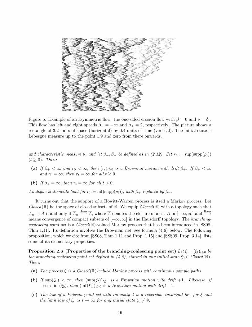
Figure 5: Example of an asymmetric flow: the one-sided erosion flow with β = 0 and ν = δ1.This flow has left and right speeds β− = −∞ and β+ = 2, respectively. The picture shows arectangle of 3.2 units of space (horizontal) by 0.4 units of time (vertical). The initial state isLebesgue measure up to the point 1.9 and zero from there onwards.
and characteristic measure ν, and let β−, β+ be defined as in (2.12). Set rt := sup(supp(ρt))(t ≥ 0). Then:
(a) If β+ < ∞ and r0 < ∞, then (rt)t≥0 is a Brownian motion with drift β+. If β+ < ∞and r0 =∞, then rt =∞ for all t ≥ 0.
(b) If β+ =∞, then rt =∞ for all t > 0.
Analogue statements hold for lt := inf(supp(ρt)), with β+ replaced by β−.
It turns out that the support of a Howitt-Warren process is itself a Markov process. LetClosed(R) be the space of closed subsets of R. We equip Closed(R) with a topology such thatAn → A if and only if An
Haus−→ A, where A denotes the closure of a set A in [−∞,∞] and Haus−→means convergence of compact subsets of [−∞,∞] in the Hausdorff topology. The branching-coalescing point set is a Closed(R)-valued Markov process that has been introduced in [SS08,Thm 1.11]. Its definition involves the Brownian net; see formula (4.6) below. The followingproposition, which we cite from [SS08, Thm 1.11 and Prop. 1.15] and [SSS09, Prop. 3.14], listssome of its elementary properties.
Proposition 2.6 (Properties of the branching-coalescing point set) Let ξ = (ξt)t≥0 bethe branching-coalescing point set defined in (4.6), started in any initial state ξ0 ∈ Closed(R).Then:
(a) The process ξ is a Closed(R)-valued Markov process with continuous sample paths.
(b) If sup(ξ0) < ∞, then (sup(ξt))t≥0 is a Brownian motion with drift +1. Likewise, if−∞ < inf(ξ0), then (inf(ξt))t≥0 is a Brownian motion with drift −1.
(c) The law of a Poisson point set with intensity 2 is a reversible invariant law for ξ andthe limit law of ξt as t→∞ for any initial state ξ0 6= ∅.
16
(d) For each deterministic time t > 0, a.s. ξt is a locally finite subset of R.
(e) Almost surely, there exists a dense set T ⊂ (0,∞) such that for each t ∈ T , the set ξtcontains no isolated points.
Our next result shows how Howitt-Warren processes and the branching-coalescing point setare related. Note that this result covers all possible values of β−, β+, except the case β− = β+
which corresponds to the Arratia flow. In (2.13) below, we continue to use the notationaA+ b := ax+ b : x ∈ A.
Theorem 2.7 (Support process) Let (ρt)t≥0 be a Howitt-Warren process with drift β andcharacteristic measure ν and let β−, β+ be defined as in (2.12). Then:
(a) If −∞ < β− < β+ <∞, then a.s. for all t > 0,
supp(ρt) = 12(β+ − β−)ξt + 1
2(β− + β+)t, (2.13)
where (ξt)t≥0 is a branching-coalescing point set.
(b) If β− = −∞ and β+ < ∞, then a.s. supp(ρt) = (−∞, rt] ∩ R for all t > 0, wherert := sup(supp(ρt)). An analogue statement holds when β− > −∞ and β+ =∞.
(c) If β− = −∞ and β+ =∞, then a.s. supp(ρt) = R for all t > 0.
Proposition 2.6 (d) and Theorem 2.7 (a) imply that if the left and right speeds of aHowitt-Warren process are finite, then at deterministic times the process is purely atomic.The next theorem generalizes this statement to any Howitt-Warren process, but shows that ifthe characteristic measure puts mass on the open interval (0, 1), then there are random timeswhen the statement fails to hold.
Theorem 2.8 (Atomicness) Let (ρt)t≥0 be a Howitt-Warren process with drift β and char-acteristic measure ν. Then:
(a) For each t > 0, the measure ρt is a.s. purely atomic.
(b) If∫
(0,1) ν(dq) > 0, then a.s. there exists a dense set of random times t > 0 when ρt ispurely non-atomic.
(c) If∫
(0,1) ν(dq) = 0, then a.s. ρt is purely atomic at all t > 0.
In the special case that ν is (a multiple of) Lebesgue measure, a weaker version of part (a)has been proved in [LR04b, Prop. 9 (c)]. Part (b) is similar to Proposition 2.6 (e) and infact, by Theorem 2.7 (a), implies the latter. Note that parts (b) and (c) of the theoremreveal an interesting dichotomy between erosion flows (where ν is nonzero and concentratedon 0, 1) and all other Howitt-Warren flows (except the Arratia flow, for which atomicness istrivial). The reason is that atoms in erosion flows lose mass continuously (see the footnote inSection 1.3 and the construction in Section 3.4 below), while in all other flows atoms can besplit into smaller atoms. This latter mechanism turns out to be more effective at destroyingatoms. For erosion flows, we have an exact description of the set of space-time points where(ρt)t≥0 has an atom in terms of an underlying Brownian web, see Theorem 9.6 below.
17
2.4 Infinite starting measures and discrete approximation
The ergodic behavior of the branching-coalescing point set is well-understood (see Proposition2.6 (c)). As a consequence, by Theorem 2.7 (a), it is known that if we start a Howitt-Warrenprocess with left and right speeds β− = −1, β+ = 1 in any nonzero initial state, then itssupport will converge in law to a Poisson point process with intensity 2. This does not mean,however, that the Howitt-Warren process itself converges in law. Indeed, since its 1-pointmotion is Brownian motion, it is easy to see that any Howitt-Warren process started in afinite initial measure satisfies limt→∞ E[ρt(K)] = 0 for any compact K ⊂ R. To find nontrivialinvariant laws, we must start the process in infinite initial measures.
To this aim, let Mloc(R) denote the space of locally finite measures on R, endowed withthe vague topology. Let (Ks,t)s≤t be a version of the Howitt-Warren flow with −∞ < β− andβ+ <∞, which satisfies Proposition 2.3 (iv). We will prove that for any ρ0 ∈Mloc(R),
ρt :=∫ρ0(dx)K0,t(x, · ) (t ≥ 0) (2.14)
defines an Mloc(R)-valued Markov process. If β+ − β− =∞, then mass can spread infinitelyfast, hence we cannot define the Howitt-Warren process (ρt)t≥0 for arbitrary ρ0 ∈ Mloc(R).In this case, we will use the class
Mg(R) :=ρ ∈Mloc(R) :
∫Re−cx
2ρ(dx) <∞ for all c > 0
, (2.15)
endowed with the topology that µn → µ if and only if e−cx2µn(dx) converges weakly to
e−cx2µ(dx) for all c > 0, which can be seen to be equivalent to µn → µ in the vague topology
plus∫e−cx
2µn(dx) →
∫e−cx
2µ(dx) for all c > 0. Note that Mloc(R) and Mg(R) are Polish
spaces.Observe that by Definition 2.1 (i), the Howitt-Warren process (ρt)t≥0 defined in (2.14)
satisfiesρt =
∫ρs(dx)Ks,t(x, ·) a.s. (2.16)
for each deterministic s < t. We will also use (2.16) to define Howitt-Warren processes startingat any deterministic time s ∈ R.
Theorem 2.9 (Infinite starting mass and continuous dependence) Let β ∈ R, let ν bea finite measure on [0, 1], and let (Ks,t)s≤t be a version of the Howitt-Warren flow with driftβ and characteristic measure ν satisfying property (iv) from Proposition 2.3. Then:
(a) For any ρ0 ∈ Mg(R), formula (2.14) defines an Mg(R)-valued Markov process withcontinuous sample paths, satisfying
E[ρt(K)] <∞ (t ≥ 0, K ⊂ R compact). (2.17)
Moreover, if (ρ〈n〉t )t≥sn are processes started at times sn with deterministic initial data ρ〈n〉sn ,
and sn → 0, then for any t > 0 and tn → t,
ρ〈n〉sn =⇒n→∞
ρ0 implies ρ〈n〉tn =⇒
n→∞ρt a.s., (2.18)
where ⇒ denotes convergence in Mg(R).
(b) Assume moreover that β+−β− <∞. Then, for any ρ0 ∈Mloc(R), formula (2.14) definesan Mloc(R)-valued Markov process with continuous sample paths. Moreover, formula (2.18)holds with convergence in Mg(R) replaced by vague convergence in Mloc(R).
18
Remark. The convergence in (2.18) implies the continuous dependence of the law of ρton the starting time and the initial law, which is known as the Feller property. Note thatwhen ρ0 is a finite measure, the continuity in t of ρt in the space M(R) already follows fromProposition 2.3 (iv). However, for our purposes, we will only consider the spaces Mg andMloc .
Remark. When β+ − β− = ∞, (ρt)t>0 may not be well-defined if ρ0 /∈ Mg(R). Indeed, byTheorem 2.7, if β+ − β− = ∞, then for any fixed t > 0, we can find xn ∈ Z with |xn| → ∞such that P(K0,t(xn, [0, 1]) < εn) < 2−n for some εn > 0. Therefore ρ0 :=
∑n ε−1n δxn has
ρ0 ∈Mloc(R), and almost surely, ρt([0, 1]) =∞.
Remark. Theorems 2.5, 2.7, and 2.8 carry over without change to the case of infinite startingmeasures. To see this, note that it is easy to check from (2.14) that
ρ0 ρ0 implies ρt ρt (t ≥ 0), (2.19)
where denotes absolute continuity. Since for each ρ0 ∈Mloc(R), we can find a finite measureρ′0 that is equivalent to ρ, statements about the support of ρt and atomicness immediatelygeneralize to the case of locally finite starting measures.
We also collect here a discrete approximation result for Howitt-Warren processes.
Theorem 2.10 (Convergence of discrete Howitt-Warren processes) Let εk be positiveconstants converging to zero, and let µk be probability measures on [0, 1] satisfying (1.7) forsome real β and finite measure ν on [0, 1]. Let (ρ〈k〉t )t≥0 be a discrete Howitt-Warren processwith characteristic measure µk defined as in (1.5), where Kω
0,t(x, ·) therein is defined for allt > 0 by letting the random walk (Xt)t≥0 in (1.1) be linearly interpolated between integer times.Let ρ〈k〉t (dx) := ρ
〈k〉ε−2k t
(ε−1k dx). If ρ〈k〉0 is deterministic and ρ
〈k〉0 ⇒ ρ0 in Mg(R), then for any
T > 0,(ρ〈k〉t )0≤t≤T =⇒
k→∞(ρt)0≤t≤T , (2.20)
where ρt is a Howitt-Warren process with drift β, characteristic measure ν, and initial con-dition ρ0, and ⇒ denotes weak convergence in law of random variables taking values inC([0, T ],Mg(R)), the space of continuous functions from [0, T ] to Mg(R) equipped with theuniform topology.
2.5 Ergodic properties
We are now ready to discuss the ergodic behavior of Howitt-Warren processes. Note that fora given Howitt-Warren flow (Ks,t)s≤t, the right-hand side of (2.14) is a.s. a linear functionof the starting measure ρ0. In view of this, Howitt-Warren processes belong to the class ofso-called linear systems. The theory of linear systems on Zd has been developed by Liggettand Spitzer, see e.g. [LS81] and [Lig05, Chap. IX]. We will adapt this theory to the continuumsetting here. First we define the necessary notion.
We let I denote the set of invariant laws of a given Howitt-Warren processes, i.e., I is the setof probability laws Λ onMloc(R) (resp.Mg(R) if β+−β− =∞) such that P[ρ0 ∈ · ] = Λ impliesP[ρt ∈ · ] = Λ for all t ≥ 0. We let T denote the set of homogeneous (i.e., translation invariant)laws on Mloc(R) (resp. Mg(R)), i.e., laws Λ such that P[ρ ∈ · ] = Λ implies P[Taρ ∈ · ] = Λfor all a ∈ R, where Taρ(A) := ρ(A + a) denotes the spatial shift map. Note that I and T
19
are both convex sets. We write Ie, Te, and (I ∩ T )e to denote respectively the set of extremalelements in I, T , and I ∩ T . Below, Cc(R) denotes the space of continuous real function onR with compact support.
Theorem 2.11 (Homogeneous invariant laws for Howitt-Warren processes) Let β ∈R, let ν be a finite measure on [0, 1] with ν 6= 0. Then for the corresponding Howitt-Warrenprocess (ρt)t≥0, we have:
(a) (I ∩ T )e is a one-parameter familly Λc : c ≥ 0 of measures satisfying Λc(d(cρ)) =Λ1(dρ) for all c ≥ 0, and∫
Λ1(dρ)∫ρ(dx)φ(x) =
∫φ(x) dx, (2.21)∫
Λ1(dρ)∫ρ(dx)φ(x)
∫ρ(dy)ψ(y) =
∫φ(x) dx
∫ψ(y) dy +
∫φ(x)ψ(x) dx2ν([0, 1])
(2.22)
for any φ, ψ ∈ Cc(R).
(b) If P[ρ0 ∈ · ] ∈ Te and E[ρ0([0, 1])] = c ≥ 0, then P[ρt ∈ · ] converges weakly to Λc.Furthermore, if E[ρ0([0, 1])2] <∞, then for any φ, ψ ∈ Cc(R),
limt→∞
E[ ∫
ρt(dx)φ(x)∫ρt(dy)ψ(y)
]=∫
Λc(dρ)∫ρ(dx)φ(x)
∫ρ(dy)ψ(y). (2.23)
(c) If P[ρ0 ∈ · ] ∈ Te and E[ρ0([0, 1])] = ∞, then the laws P[ρt ∈ · ] have no weak clusterpoint as t→∞ which is supported on Mloc(R).
(d) If Λ ∈ I ∩ T , then there exists a probability measure γ on [0,∞) such that Λ =∫∞0 γ(dc) Λc.
Remark. When ν is Lebesgue measure, it is known that (see [LR04b, Prop. 9 (b)]) Λc is thelaw of cρ∗, where ρ∗ =
∑(x,u)∈P uδx for a Poisson point process P on R× [0,∞) with intensity
measure dx× u−1e−udu.
Theorem 2.11 shows that each Howitt-Warren process has a unique (modulo a constant multi-ple) homogeneous invariant law, which by (2.22) has zero off-diagonal correlations. Moreover,any ergodic law at time 0 with finite density converges under the dynamics to the uniquehomogeneous invariant law with the same density.
In line with Theorems 2.7 and 2.8 we have the following support properties for Λc.
Theorem 2.12 (Support of stationary process) Let c > 0 and let ρ be anMloc(R)-valuedrandom variable with law Λc, the extremal homogeneous invariant law defined in Theorem 2.11.Then:
(a) If β+ − β− <∞, then supp(ρ) is a Poisson point process with intensity β+ − β−.
(b) If β+ − β− =∞, then ρ is a.s. atomic with supp(ρ) = R.
20
3 Construction of Howitt-Warren flows in the Brownian web
In this section, we make the heuristics in Section 1.3 rigorous and give a graphical constructionof the Howitt-Warren flows using a procedure of Poisson marking of the Brownian web inventedby Newman, Ravishankar and Schertzer [NRS10]. The random environment for the Howitt-Warren flow will turn out to be a Brownian web, which we call the reference web, plus amarked Poisson point process on the reference web. Given such an environment, we will thenconstruct a second coupled Brownian web, which we call the sample web, which is constructedby modifying the reference web by switching the orientation of marked points of type (1, 2).The kernels of the Howitt-Warren flow are then constructed from the quenched law of thesample web, conditional on the reference web and the associated marked Poisson point process.
This construction generalizes the construction of the erosion flow based on coupled Brow-nian webs given in [HW09b]. For erosion flows, the random environment consists only of areference web (without marked points) and the construction of the sample web can be doneby specifying the joint law of the reference web and the sample web by means of a martingaleproblem. This is the approach taken in [HW09b]. In the general case, when the randomenvironment also contains marked points, this approach does not work. Therefore, in ourapproach, even for erosion flows, we will give a graphical construction of the sample web bymarking and switching paths in the reference web.
Discrete approximation will be an important tool in many of our proofs and is helpfulfor understanding the continuum models. Therefore, in Section 3.1, we will first formulatethe notion of a quenched law of sample webs conditional on the random environment fordiscrete Howitt-Warren flows. In Section 3.2, we then recall the necessary background onthe Brownian web and Poisson marking for the Brownian web. In Section 3.3, we showhow coupled Brownian webs can be constructed by Poisson marking and switching paths in areference web. In Section 3.4, we state our main result, Theorem 3.7, which is the constructionof Howitt-Warren flows using the Poisson marking of a reference Brownian web, and we alsostate some regularity properties for the Howitt-Warren flows. Lastly, in Section 3.5, we statea convergence result on the quenched law of discrete webs, which will be used to identifythe flows we construct in Theorem 3.7 as being, indeed, the Howitt-Warren flows defined inSection 2.2 earlier through their n-point motions. The statements of this section are provedin Sections 6 and 7.
3.1 A quenched law on the space of discrete webs
As in Section 1.2, let ω := (ωz)z∈Z2even
be i.i.d. [0, 1]-valued random variables with commondistribution µ. Instead of using ω as a random environment for a single random walk startedfrom one fixed time and position, as we did in Section 1.2, we will now use ω as a randomenvironment for a collection of coalescing random walks starting from each point in Z2
even. Tothis aim, conditional on ω, let α = (αz)z∈Z2
evenbe a collection of independent −1,+1-valued
random variables such that αz = +1 with probability ωz and αz = −1 with probability 1−ωz.This α will play a somewhat different role from the α〈k〉 in Section 1.3; see the discussionbelow Theorem 3.7. For each (x, s) ∈ Z2
even, we let pα(x,s) : s, s + 1, . . . → Z be the functionpα(x,s) = p defined by
p(s) := x and p(t+ 1) := p(t) + α(p(t),t) (t ≥ s). (3.1)
21
Then pα(x,s) is the path of a random walk in the random environment ω, started at time s atposition x. It is easy to see that paths pαz , p
αz′ starting at different points z, z′ coalesce when
they meet. We call the collection of paths
Uα := pαz : z ∈ Z2even (3.2)
the discrete web associated with α (see Figure 6), where starting from this section, for the restof the paper, we will use different notation for discrete webs and nets compared to Section 1.2,to avoid confusion with certain other symbols that we will need. Let P denote the law of ωand let
Qω := P[Uα ∈ ·
∣∣ω] (3.3)
denote the conditional law of Uα given ω. Then under the averaged law∫
P(dω)Qω, pathsin Uα are coalescing random walks that in each time step jump to the right with probability∫µ(dq)q and to the left with the remaining probability
∫µ(dq)(1− q).
Figure 6: A discrete web and its dual.
We will be more interested in the quenched law Qω defined in (3.3). One has
Qωz = Qω[pαz ∈ · ] (3.4)
where Qωz is the conditional law of the random walk in random environment started from
z ∈ Z2even defined in Section 1.2. In particular, by (1.1),
Kωs,t(x, y) = Qω
[pα(x,s)(t) = y
]= P
[pα(x,s)(t) = y
∣∣ω] ((x, s), (y, t) ∈ Z2
even
), (3.5)
where (Kωs,t)s≤t is the discrete Howitt-Warren flow with characteristic measure µ. In view of
this, the random law Qω contains all information that we are interested in. We call Qω thediscrete quenched law with characteristic measure µ. In the next sections, we will construct acontinuous analogue of this quenched law and use it to define Howitt-Warren flows.
3.2 The Brownian web
As pointed out in the previous subsection, under the averaged law∫
P(dω)Qω, the discrete webUα is a collection of coalescing random walks, started from every point in Z2
even. It turns out
22
that such discrete webs have a well-defined diffusive scaling limit, which is basically a collectionof coalescing Brownian motions, starting from each point in space and time, and which is calleda Brownian web. The Brownian web arose from the work of Arratia [Arr79, Arr81] and hassince been studied by Toth and Werner [TW98]. More recently, Fontes, Isopi, Newman andRavishankar [FINR04] have introduced a by now standard framework in which the Brownianweb is regarded as a random compact set of paths, and is an element of a suitable Polishspace.
It turns out that associated to each Brownian web, there is a dual Brownian web, which isa collection of coalescing Brownian motions running backwards in time. To understand thison a heuristic level, let (αz)z∈Z2
evenbe an i.i.d. collection of −1,+1-valued random variables.
If for each z = (x, t) ∈ Z2even, we draw an arrow from (x, t) to (x + αz, t + 1), then paths
along these arrows form a discrete web as introduced in the previous section. Now, if foreach z = (x, t) ∈ Z2
even, we draw in addition a dual arrow from (x, t + 1) to (x − αz, t), thenpaths along these dual arrows form a dual discrete web of coalescing random walks runningbackwards in time, which do not cross paths in the forward web (see Figure 6). The dualBrownian web arises as the diffusive scaling limit of such a dual discrete web.
We now introduce these objects formally. Let R2c be the compactification of R2 obtained
by equipping the set R2c := R2 ∪ (±∞, t) : t ∈ R ∪ (∗,±∞) with a topology such that
(xn, tn) → (±∞, t) if xn → ±∞ and tn → t ∈ R, and (xn, tn) → (∗,±∞) if tn → ±∞(regardless of the behavior of xn). An explicit way to construct such a compactification is asfollows. Let Θ : R2 → R2 be defined by
Θ(x, t) =(Θ1(x, t),Θ2(t)
):=(tanh(x)
1 + |t|, tanh(t)
), (3.6)
and let Θ(R2) denote the image of R2 under Θ. Then the closure of Θ(R2) in R2 is in a naturalway isomorphic to R2
c (see Figure 7).
t
t
tt
t(∗,−∞)
(∗,+∞)
(0, 0)
(+∞, 2)
(−∞,−1)
Figure 7: The compactification R2c of R2.
By definition, a path π in R2c with starting time σπ is a function π : [σπ,∞]→ [−∞,∞]∪∗
such that t 7→ (π(t), t) is a continuous map from [σπ,∞] to R2c . We will often view paths as
subsets of R2c , i.e., we identify a path π with its graph (π(t), t) : t ∈ [σπ,∞]. We let Π
denote the space of all paths in R2c with all possible starting times in [−∞,∞], equipped with
23
the metric
d(π1, π2) := |Θ2(σπ1)−Θ2(σπ2)| ∨ supt≥σπ1∧σπ2
∣∣Θ1
(π1(t ∨ σπ1), t)−Θ1(π2(t ∨ σπ2), t
)∣∣, (3.7)
and we let K(Π) denote the space of all compact subsets K ⊂ Π, equipped with the Hausdorffmetric
dH(K1,K2) = supx1∈K1
infx2∈K2
d(x1, x2) ∨ supx2∈K2
infx1∈K1
d(x1, x2). (3.8)
Both Π and K(Π) are complete separable metric spaces. The set Π of all dual paths π :[−∞, σπ]→ [−∞,∞] ∪ ∗ with starting time σπ ∈ [−∞,∞] is defined analoguously to Π.
We adopt the convention that if f : R2c → R2
c and A ⊂ R2c , then f(A) := f(z) : z ∈ A
denotes the image of A under f . Likewise, if A is a set of subsets of R2c (e.g. a set of paths),
then f(A) := f(A) : A ∈ A. This also applies to notation such as −A := −z : z ∈ A. IfA ⊂ Π is a set of paths and A ⊂ R2
c , then we let A(A) := π ∈ A : (π(σπ), σπ) ∈ A denote thesubspace of all paths in A with starting points in A, and for z ∈ R2
c we write A(z) := A(z).The next proposition, which follows from [FINR04, Theorem 2.1], [FINR06, Theorem 3.7],
and [SS08, Theorem 1.9], gives a characterization of the Brownian web W and its dual W.Below, we say that a path π ∈ Π crosses a dual path π ∈ Π from left to right if there existσπ ≤ s < t ≤ σπ such that π(s) < π(s) and π(t) < π(t). Crossing from right to left is definedanalogously.
Proposition 3.1 (Characterization of the Brownian web and its dual) For each β ∈R, there exists a K(Π) × K(Π)-valued random variable (W, W), called the double Brownianweb with drift β, whose distribution is uniquely determined by the following properties:
(a) For each deterministic z ∈ R2, almost surely there is a unique path πz ∈ W(z) and aunique dual path πz ∈ W(z).
(b) For any deterministic countable dense subset D ⊂ R2, almost surely, W is the closurein Π of πz : z ∈ D and W is the closure in Π of πz : z ∈ D.
(c) For any finite deterministic set of points z1, . . . , zk ∈ R2, the paths (πz1 , . . . , πzk) aredistributed as a collection of coalescing Brownian motions, each with drift β.
(d) For any deterministic z ∈ R2, the dual path πz is the a.s. unique path in Π(z) that doesnot cross any path in W.
If (W, W) is a double Brownian web as defined in Proposition 3.1, then we callW a Brownianweb and W the associated dual Brownian web. Note that W is a.s. uniquely determined byW.Although this is not obvious from the definition, the dual Brownian web is indeed a Brownianweb rotated by 180 degrees. Indeed, (W, W) is equally distributed with (−W,−W).
Definition 3.2 (Incoming and outgoing paths) We say that a path π ∈ Π is an incomingpath at a point z = (x, t) ∈ R2 if σπ < t and π(t) = x. We say that π is an outgoing path atz if σπ = t and π(t) = x. We say that two incoming paths π1, π2 at z are strongly equivalent,denoted as π1 =z
in π2, if π1 = π2 on [t − ε, t] for some ε > 0. For z ∈ R2, let min(z) denotethe number of equivalence classes of incoming paths in W at z and let mout(z) denote thecardinality of W(z). Then (min(z),mout(z)) is called the type of the point z in W. The type(min(z), mout(z)) of a point z in the dual Brownian web W is defined analogously.
24
We cite the following result from [TW98, Proposition 2.4] or [FINR06, Theorems 3.11–3.14]. See Figure 8 for an illustration.
Proposition 3.3 (Special points of the Brownian web) Almost surely, all points z ∈ R2
are of one of the following types in W/W: (0, 1)/(0, 1), (0, 2)/(1, 1), (0, 3)/(2, 1), (1, 1)/(0, 2),(1, 2)/(1, 2), and (2, 1)/(0, 3). For each deterministic t ∈ R, almost surely, each point inR × t is of type (0, 1)/(0, 1), (0, 2)/(1, 1), or (1, 1)/(0, 2). Deterministic points z ∈ R2 area.s. of type (0, 1)/(0, 1).
Figure 8: Special points of the Brownian web. On the left: (0, 1)/(0, 1). Top row: (1, 1)/(0, 2),(2, 1)/(0, 3), (1, 2)l/(1, 2)l. Bottom row: (0, 2)/(1, 1), (0, 3)/(2, 1), (1, 2)r/(1, 2)r.
For us, points of type (1, 2)/(1, 2) are of special importance. Note that these are the onlypoints at which there are incoming paths both in W and in W. Points of type (1, 2) in W arefurther distinguished into points of type (1, 2)l and (1, 2)r, according to whether the left orthe right outgoing path in W is the continuation of the (up to equivalence unique) incomingpath.
Proposition 3.3 shows that although for each deterministic z ∈ R2, a.s. W(z) contains asingle path, there exist random points z where W(z) contains up to three paths. Sometimes,it will be necessary to choose a unique element of W(z) for each z ∈ R2. To that aim, foreach z ∈ R2, we let π+
z denote the right-most element of W(z). We define π↑z in the same way,except that at points of type (1, 2)l, we let π↑z be the left-most element of W(z). Note thatas a consequence of this choice, whenever there are incoming paths at z, the path π↑z is thecontinuation of any incoming path at z.
The next proposition, which follows from [NRS10, Prop. 3.1], shows that it is possible todefine something like the intersection local time ofW and W. Below, |I| denotes the Lebesguemeasure of a set I ⊂ R.
Proposition 3.4 (Intersection local time) Let (W, W) be the double Brownian web. Thena.s. there exists a unique measure `, concentrated on the set of points of type (1, 2) in W, suchthat for each π ∈ W and π ∈ W,
`(z = (x, t) ∈ R2 : σπ < t < σπ, π(t) = x = π(t)
)= lim
ε↓0ε−1∣∣t ∈ R : σπ < t < σπ, |π(t)− π(t)| ≤ ε
∣∣, (3.9)
25
where the limit on the right-hand side exists and is finite. The measure ` is a.s. non-atomicand σ-finite. We let `l and `r denote the restrictions of ` to the sets of points of type (1, 2)l
and (1, 2)r, respectively.
We remark that `(O) = ∞ for every open nonempty subset O ⊂ R2, but ` is σ-finite. Tosee the latter, for any path π ∈ Π, let π := (π(t), t) : t ∈ (σπ,∞) denote its interior,and define the interior π of a dual path π ∈ Π analogously. Let D ⊂ R2 be a deterministiccountable dense set and for z ∈ D, let πz, resp. πz, denote the a.s. unique path inW, resp. W,starting from z. Then by Proposition 3.4, `(πz ∩ πz) < ∞ for each z, z ∈ D, while by [SS08,Lemma 3.4 (b)], ` is concentrated on
⋃z,z∈D(πz ∩ πz).
3.3 Sticky Brownian webs
We collect here some facts about a natural way to couple two Brownian webs. Such coupledBrownian webs will then be used in the next subsection to give a graphical construction ofHowitt-Warren flows. We first start with a ‘reference’ Brownian webW, which is then used toconstruct a second, ‘modified’ or ‘sample’ Brownian web W ′ by ‘switching’ a suitable Poissonsubset of points of type (1, 2)l ofW into points of type (1, 2)r, and vice versa, using a markingprocedure developed in [NRS10].
To formulate this rigorously, let z = (x, t) be a point of type (1, 2)l in W, and let
Win(z) := π ∈ W : σπ < t, π(t) = x (3.10)
denote the set of incoming paths in W at z. For any π ∈ Win(z), let πt := (π(s), s) : σπ ≤s ≤ t denote the piece of π leading up to z, and let W(z) = l, r be the outgoing paths inW at z, where l < r on (t, t+ ε) for some ε > 0. Since z is of type (1, 2)l, identifying a pathwith its graph, we have π = πt ∪ l for each π ∈ Win(z). We define
switchz(W) :=(W\Win(z)
)∪ πt ∪ r : π ∈ Win(z). (3.11)
Then switchz(W) differs from W only in that z is now of type (1, 2)r instead of (1, 2)l. In asimilar way, if z is of type (1, 2)r in W, then we let switchz(W) denote the web obtained fromW by switching z into a point of type (1, 2)l. If z1, . . . , zn are points of type (1, 2) in W, thenwe let switchz1,...,zn(W) := switchz1 · · · switchzn(W) denote the web obtained from W byswitching the orientation of the points z1, . . . , zn. Note that it does not matter in which orderwe perform the switching. Recall that a point z is of type (1, 2)l (resp. (1, 2)r) in the dualBrownian web W if and only if it is of type (1, 2)l (resp. (1, 2)r) in W. We define switching inW analogously to switching in W.
The next theorem, which is similar to [NRS10, Prop. 6.1], shows how by switching theorientation of a countable Poisson set of points of type (1, 2), we can obtain a well-definedmodified Brownian web. Recall the definition of the intersection local time measure ` fromProposition 3.4 and note that since ` is σ-finite, the set S below is a.s. a countable subset ofthe set of all points of type (1, 2).
Theorem 3.5 (Modified Brownian web) Let W be a Brownian web wih drift β, let ` bethe intersection local time measure between W and its dual and let `l, `r denote the restrictionsof ` to the sets of points of type (1, 2)l and (1, 2)r in W, respectively. Let cl, cr ≥ 0 be constants
26
and conditional on W, let S be a Poisson point set with intensity cl`l + cr`r. Then, a.s., forany sequence of finite sets ∆n ↑ S, the limit
(W ′, W ′) := lim∆n↑S
(switch∆n(W), switch∆n(W)
)(3.12)
exists in K(Π)×K(Π) and does not depend on the choice of the sequence ∆n ↑ S. Moreover,W ′ is a Brownian web with drift β′ = β + cl − cr and W ′ is its dual.
Remark. We recall that a countable set S ⊂ R2 is a Poisson point set with σ-finite intensityµ if S∩An a Poisson point set with intensity µ(An∩ · ) for some, and hence for every sequenceof measurable sets An such that µ(An) <∞ for all n and µ(R2\
⋃nAn) = 0. We apply this to
the case that µ is the random measure cl`l +cr`r and the An are finite unions of intersections offorward and dual paths, started from deterministic points, as mentioned below Proposition 3.4.In particular, when we say that S is Poisson with intensity cl`l+cr`r, this should be interpretedin this particular sense. Some care is needed when talking about the conditional law of S givenW, since it is not clear whether S (being a countable dense subset of R2), on its own, can beviewed as a random variable with values in a decent (at least measurable) space. Nevertheless,it is not hard to see that the triple (W, W, S) (being a marked double Brownian web) can beconstructed as a legitimate random variable on a suitable probability space and that (W ′, W ′)is a.s. a measurable function of (W, W, S).
If (W,W ′) are coupled as in Theorem 3.5, then we say that (W,W ′) is a pair of stickyBrownian webs with drifts β, β′ and coupling parameter κ := mincl, cr. In the special casethat κ = 0 and β ≤ β′, we call (W,W ′) a left-right Brownian web with drifts β, β′. Left-rightBrownian webs have been introduced with the help of a ‘left-right stochastic differential equa-tion’ (instead of the marking construction above) in [SS08]. Pairs of sticky Brownian webswith general coupling parameters κ ≥ 0 have been introduced by means of a martingale prob-lem in [HW09b, Section 7]. They are, indeed, sticky in the sense that a pair of paths, one fromeach web, are Brownian motions with sticky interaction. We will prove in Lemma 6.18 belowthat the constructions of left-right Brownian webs given above and in [SS08] are equivalent.We will not make use of the martingale formulation of sticky Brownian webs developed in[HW09b].
For any point z of type (1, 2) in some Brownian web W, we call
signW(z) :=−1 if z is of type (1, 2)l in W,+1 if z is of type (1, 2)r in W (3.13)
the sign of z in W. If (W,W ′) is a pair of sticky Brownian webs, then it is known [SSS09,Thm. 1.7] that the set of points of type (1, 2) in W in general does not coincide with the setof points of type (1, 2) in W ′. The next proposition says that nevertheless, in the sense ofintersection local time measure, almost all points of type (1, 2) in W are also of type (1, 2) inW ′, and these point have the orientation one expects.
Proposition 3.6 (Change of reference web) In the setup of Theorem 3.5, let `′ be theintersection local time measure between W ′ and its dual and let `′l, `
′r denote the restrictions
of `′ to the sets of points of type (1, 2)l and (1, 2)r in W ′, respectively. Then:
(i) Almost surely, `′l = `l and `′r = `r.
(ii) S =z ∈ R2 : z is of type (1, 2) in both W and W ′, and signW(z) 6= signW ′(z)
a.s.
27
(iii) Conditional on W ′, the set S is a Poisson point set with intensity cr`′l + cl`
′r and W =
lim∆n↑S switch∆n(W ′).
Let (W0,W) be a pair of sticky Brownian webs with drifts β0, β and coupling parameterκ, and let π↑z and π+
z denote the special paths in W(z) defined below Proposition 3.3. Let
K↑s,t(x,A) := P[π↑(x,s)(t) ∈ A
∣∣W0
] (s ≤ t, x ∈ R, A ∈ B(R)
), (3.14)
and let K+s,t(x,A) be defined similarly, with π↑z replaced by π+
z . Then, as we will see inTheorem 3.7 below, (K↑s,t)s≤t and (K+
s,t)s≤t are versions of the Howitt-Warren flow with driftβ and characteristic measure ν = clδ1 + crδ0, where
In the special case that cl = cr, this was proved in [HW09b, formula (5)]. In the nextsubsection, we set out to give a similar construction for any Howitt-Warren flow.
3.4 Marking construction of Howitt-Warren flows
We now give a construction of a general Howitt-Warren flow based on two coupled webs, whichis the central result of this paper. More precisely, the random environment of the Howitt-Warren flow will be represented by a reference Brownian web W0 plus a set M of markedpoints of type (1, 2). Conditional on (W0,M), we will modify W0 in a similar way as inTheorem 3.5 to construct a sample Brownian webW, whose law conditional on (W0,M) thendefines the Howitt-Warren flow via the continuous analogue of (3.5). For erosion flows, theset M of marked points is empty, hence our representation reduces to (3.14).
Let W0 be a Brownian web with drift β0 and let νl and νr be finite measures on [0, 1].Let `, `l and `r be defined for W0 as in Proposition 3.4, and conditional on W0, let M be aPoisson point set on R2 × [0, 1] with intensity
Elements of M are pairs (z, q) where z is a point of type (1, 2) in W0 and q ∈ [0, 1]. Since `is non-atomic, for each point z of type (1, 2) there is at most one q such that (z, q) ∈M, andwe may writeM = (z, ωz) : z ∈M. We call points z ∈M marked points and we call ωz themark of z.
Conditional on the reference web W0 and the set of marked points M, we constructindependent −1,+1-valued random variables (αz)z∈M with P[αz = +1|(W0,M)] = ωz, andwe set
A := z ∈M : αz 6= signW0(z). (3.17)
In addition, conditional on (W0,M), we let B be a Poisson point set with intensity 2νl(0)`l+2νr(1)`r, independent of A. We observe that conditional on W0, but integrating out therandomness of M, the set A ∪B is a Poisson point set with intensity
2(∫
(0,1]qq−1νl(dq) + νl(0)
)`l + 2
(∫[0,1)
(1− q)(1− q)−1νr(dq) + νr(1))`r
= 2νl
([0, 1]
)`l + 2νr
([0, 1]
)`r.
(3.18)
28
Therefore, by Theorem 3.5, a.s. the limit
W := lim∆n↑A∪B
switch∆n(W0) (3.19)
exists in K(Π) and is a Brownian web with drift
β := β0 + 2νl
([0, 1]
)− 2νr
([0, 1]
). (3.20)
Theorem 3.7 (Construction of Howitt-Warren flows) Let β ∈ R and let ν be a finitemeasure on [0, 1]. For any finite measures νl and νr on [0, 1] satisfying
ν(dq) := (1− q)νl(dq) + qνr(dq), (3.21)
let β0 be determined from β, νl and νr as in (3.20). Let W0 be a reference Brownian web withdrift β0 and define a set of marked points M and sample Brownian web W as in (3.16) and(3.19). Let π↑z and π+
z denote the special paths in W(z) defined below Proposition 3.3. Set
K↑s,t(x,A) := P[π↑(x,s)(t) ∈ A
∣∣ (W0,M)] (
s ≤ t, x ∈ R, A ∈ B(R))
(3.22)
and define K+s,t(x,A) similarly with π↑(x,s) replaced by π+
(x,s). Then (K↑s,t)s≤t and (K+s,t)s≤t are
versions of the Howitt-Warren flow with drift β and characteristic measure ν. In the specialcase that νl = νr, the triple (W0,M,W) is equally distributed with (W,M,W0).
Remark. Since W take values in the Polish space K(Π), we may construct a regular versionof the conditional probability P[W ∈ · |(W0,M)], which is a random probability measure onK(Π). A.s., under this random law, the random set of paths W has the same a.s. propertiesas a Brownian web. In particular, for a.e. ω in our underlying probability space, the pathsπ↑z and π+
z in W are well-defined for all z ∈ R2 and we obtain a version of the conditionalprobabilities in formula (3.22) for all (x, s) ∈ R2 and t ≥ s simultaneously. Interpretingformula (3.22) in this way (as we will always do), we obtain versions (K↑s,t)s≤t and (K+
s,t)s≤tof our Howitt-Warren flows with different properties, see Proposition 3.8 below.
Remark. Note that in (3.21), it is always possible to choose νl = νr = ν. In this case, theconstruction of the reference Brownian web and set of marked points arises as the scaling limitof the discrete construction outlined in Section 1.3. If ω〈k〉 = (ω〈k〉z )z∈Z2
evenis a collection of
independent [0, 1]-valued random variables with laws µk satisfying (1.7) and conditional onω〈k〉 we construct two independent collections α〈k〉 = (α〈k〉z )z∈Z2
evenand α〈k〉 = (α〈k〉z )z∈Z2
even
of −1,+1-valued random variables with P[α〈k〉z = +1 |ω〈k〉] = ω〈k〉z , and similar for α〈k〉,
then the discrete webs corresponding to α〈k〉 and α〈k〉 converge after diffusive rescaling to Wand W0, and (z, ωz) : 0 < ωz < 1 converges to the set of marked points M. The moregeneral construction in Theorem 3.7 where possibly νl 6= νr and β0 is possibly different from βarises as the diffusive scaling limit of discrete constructions where we first choose a referencecollection of random variables α〈k〉 with ε−1
k E[α〈k〉z ] → β0 and then conditional on α〈k〉, wechoose independent (ω〈k〉z )z∈Z2
evenwith P[ωz ∈ dq | α〈k〉 = −1] = µl
k(dq) and P[ωz ∈ dq | α〈k〉 =+1] = µr
k(dq), where generalizing (1.9), µlk and µr
k are any laws such that
P[α〈k〉 = −1]µlk(dq) + P[α〈k〉 = +1]µr
k(dq) = µk(dq). (3.23)
29
This more general construction will sometimes be handy. For example, for erosion flows whereν = c0δ0 + c1δ1 for some c0, c1 ≥ 0, it is most natural to choose νl = c0δ0 and νr = c1δ1. Also,for Howitt-Warren flows where one or both of the speeds β−, β+ defined in (2.12) are finite, itis sometimes handy to choose either νl = 0 or νr = 0.
If (W0,M,W) are a reference Brownian web, the set of marked points, and the sampleBrownian web as defined above Theorem 3.7, then we call the random probability measure Qon K(Π) defined by
Q := P[W ∈ ·
∣∣ (W0,M)]
(3.24)
the Howitt-Warren quenched law with drift β and characteristic measure ν. In Section 3.5below, we will show that in some precisely defined way, these Howitt-Warren quenched lawsare the diffusive scaling limits of the discrete quenched laws defined in Section 3.1.
Since at deterministic points in the Brownian web W there is a.s. only one outgoing path,the stochastic flows of kernels (K↑s,t)s≤t and (K+
s,t)s≤t from Theorem 3.7 obviously have thesame finite-dimensional distributions. They are, however, not the same. Each version has itsown pleasant properties.
Proposition 3.8 (Regular parameter dependence) Let (K↑s,t)s≤t and (K+s,t)s≤t be defined
as in Theorem 3.7. Then, of the following properties, (K+s,t)s≤t satisfies (a)–(c) and (K↑s,t)s≤t
satisfies (a), (b) and (d).
(a) Setting R2≤ := (s, t) ∈ R2 : s ≤ t, the map (s, t, x, ω) 7→ Ks,t(x, · )(ω) is a measurable
map from R2≤ × R× Ω to M1(R).
(b) A.s., the map t 7→ Ks,t(x, · ) from [s,∞) to M1(R) is continuous for all s ∈ R andx ∈ R.
(c) A.s., x 7→ Ks,t(x,A) is a cadlag function from R to R for each s < t and A ∈ B(R).
(d) A.s.,∫
RKs,t(x,dy)Kt,u(y,A) = Ks,u(x,A) for all s ≤ t ≤ u, x ∈ R, and A ∈ B(R).
Proposition 3.8 (b) and (d) show that (K↑s,t)s≤t yields a version of a Howitt-Warren flowwith the properties listed in Proposition 2.3. In particular, Proposition 3.8 (d) makes it afamily of bona fide transition probability kernels of a Markov process in a random space-timeenvironment.
3.5 Discrete approximation
Recall the definitions of the discrete quenched laws Q in (3.3) and the Howitt-Warren quenchedlaws Q in (3.24). In this subsection, we formulate a convergence result which says that if µk isa sequence of probability laws on [0, 1] satisfying (1.7), then the associated discrete quenchedlaws Q〈k〉, diffusively rescaled, converge to the Howitt-Warren quenched law Q with drift βand characteristic measure ν. This abstract result then implies other convergence results suchas the convergence of Howitt-Warren flows, Howitt-Warren processes, and n-point motions.Since the n-point motions of discrete Howitt-Warren flows will be shown in Proposition A.5to converge to solutions of the Howitt-Warren martingale problems, this will also verify thatthe flows we constructed in Theorem 3.7 are indeed versions of the Howitt-Warren flow.
To formulate our convergence statement properly, we need to identify a discrete quenchedlaw Q with a random probability law on the space K(Π) of compact subsets of the space Π
30
of paths defined in Section 3.2. Recall the definition of the paths pαz in (3.1) and the discretewebs Uα in (3.2). We wish to view Uα as a random variable with values in K(Π). To this aim,we modify our definition of Uα as follows. First, for each z = (x, s) ∈ Z2
even we make pαz (t)into a path in Π by linear interpolation between integer times and by setting pαz (∞) := ∗.Next, we add to Uα all trivial paths π, with starting times σπ ∈ Z∪ −∞,∞, such that π isidentically −∞ or +∞ on [σπ,∞) ∩ R. With this modified definition, it can be checked thatUα is indeed a random compact subset of Π, as desired.
For ε > 0, we let Sε : R2c → R2
c denote the scaling map
Sε(x, t) := (εx, ε2t)((x, t) ∈ R2
c
). (3.25)
As usual, we identify paths with their graphs; then Sε(π) is the path obtained by diffusivelyrescaling a path π with ε, and Sε(Uα) is the random collection of paths obtained by diffusivelyrescaling paths in Uα. If Qω is a discrete quenched law as defined in (3.3) and ε > 0, then wewrite
Sε(Qω) := Qω[Sε(Uα) ∈ ·
], (3.26)
i.e., Sε(Qω) is the image under the scaling map Sε of the quenched law of Uα. Note thatSε(Qω), so defined, is a random probability law on the space of compact subsets of Π, i.e., arandom variable with values in M1(K(Π)).
Theorem 3.9 (Convergence of quenched laws) Let εk be positive constants, converging tozero and µk be probability measures on [0, 1] satisfying (1.7) for some real β and finite measureν on [0, 1]. Let ω〈k〉 = (ω〈k〉z )z∈Z2
evenbe i.i.d. [0, 1]-valued random variables with distibution µk,
let Q〈k〉 := Qω〈k〉 be the discrete quenched law defined in (3.3), and let Q be the Howitt-Warrenquenched law with drift β and characteristic measure ν defined in (3.24). Then
P[Sεk(Q〈k〉) ∈ ·
]=⇒k→∞
P[Q ∈ · ], (3.27)
where ⇒ denotes weak convergence of probability laws on M1(K(Π)).
4 Construction of Howitt-Warren flows in the Brownian net
In this section, we show that when a Howitt-Warren flow with drift β and characteristicmeasure ν has finite left and right speeds, or equivalently, b :=
∫q−1(1 − q)−1ν(dq) < ∞,
then we can alternatively construct the flow as a random flow of mass in the Brownian net.Analogous to Theorem 3.7, the random environment will now be represented as a Browniannet N plus a set of i.i.d. marks ω := (ωz)z∈S attached to the separation points S of N , eachwith law ν(dq) := b−1q−1(1− q)−1ν(dq). Conditional on (N , ω), we can construct the sampleweb W by choosing trajectories in N that turn in the ‘right’ way at separation points. TheHowitt-Warren flow is then defined from the law of W conditional on (N , ω) as in (3.22).
In Sections 4.1–4.2, we recall the necessary background on the Brownian net and propertiesof its separation points. In Section 4.3, we first state some coupling results between theBrownian web and Brownian net, which will help shed more light on the marking constructionsof sticky Brownian webs in Theorem 3.5. In Section 4.4 we then give our main result on thealternative construction of Howitt-Warren flows with finite left and right speeds using theBrownian net. Lastly in Section 4.5, we formulate what we call Brownian half-nets, and statesome properties for the support of the Howitt-Warren quenched law defined in (3.24), which
31
will imply Theorems 2.5 and 2.7. We note that, apart from being used to construct Howitt-Warren flows with finite left and right speeds, the theory of the Brownian net will also play animportant role for Howitt-Warren flows with infinite left or right speed, such as in the proofof results in Section 4.5, as well as in the proof of Theorems 3.5 and 3.9.
4.1 The Brownian net
The Brownian net arises as the diffusive scaling limit of branching-coalescing random walksin the limit of small branching probability. It was first introduced by Sun and Swart in [SS08]and independently by Newman, Ravishankar and Schertzer in [NRS10]. A further study of itsproperties was carried out in [SSS09]. We now recall the definition of the Brownian net givenin [SS08].
Recall that in Section 3.3, we defined a left-right Brownian web to be a pair of stickyBrownian webs (W l,Wr) with drifts β− ≤ β+ and coupling parameter κ = 0. At present, wewill need the original definition of a left-right Brownian web given in [SS08]. In Lemma 6.18below, we will prove that both definitions are equivalent.
Following [SS08], we call (l1, . . . , lm; r1, . . . , rn) a collection of left-right coalescing Brownianmotions with drifts β− ≤ β+, if (l1, . . . , lm) and (r1, . . . , rn) are distributed as collections of co-alescing Brownian motions with drift β− and β+, respectively, if paths in (l1, . . . , lm; r1, . . . , rn)evolve independently when they are apart, and the interaction between li and rj when theymeet is described by the two-dimensional stochastic differential equation
dLt = 1Lt 6=RtdBlt + 1Lt=RtdB
st + β−dt,
dRt = 1Lt 6=RtdBrt + 1Lt=RtdB
st + β+dt,
(4.1)
where Blt, B
rt , B
st are independent standard Brownian motions, and (L,R) are subject to the
constraint thatLt ≤ Rt for all t ≥ infs : Ls = Rs. (4.2)
It can be shown that subject to the condition (4.2), solutions to the SDE (4.1) are unique indistribution [SS08, Proposition 2.1].
Let W l,Wr be two Brownian webs with drifts β− ≤ β+, and for determinstic z ∈ R2,let lz resp. rz denote the a.s. unique path in W l resp. Wr starting from z. Following [SS08],we say that (W l,Wr) is a left-right Brownian web if for any finite deterministic set of pointsz1, . . . , zm, z
′1, . . . , z
′n ∈ R2, the collection (lz1 , . . . , lzm ; rz′1 , . . . , rz′n) is distributed as left-right
coalescing Brownian motions. Elements of W l (resp. Wr) are called left-most (resp. right-most) paths. It is known [SS08, formula (1.22)] that if (W l,Wr) is a left-right Brownian weband W l, Wr are the dual Brownian webs associated with W l,Wr, then (−W l,−Wr) is equallydistributed with (W l,Wr).
It was shown in [SS08] that each left-right Brownian web a.s. determines an associatedBrownian net and vice versa. There, three different ways were given to construct a Browniannet from its associated left-right Brownian web, which are known as the hopping constructionand the constructions using wedges and meshes, which we recall now.
Hopping: We call t ∈ R an intersection time of two paths π, π′ ∈ Π if σπ, σπ′ < t < ∞and π(t) = π′(t). If t is an intersection time of π and π′, then we can define a new pathπ′′ by concatenating the piece of π before t with the piece of π′ after t, i.e., by settingπ′′ := (π(s), s) : s ∈ [σπ, t] ∪ (π′(s), s) : s ∈ [t,∞]. For any collection of paths A ⊂ Π, we
32
let Hint(A) denote the smallest set of paths containing A that is closed under such ‘hopping’from one path onto another at intersection times, i.e., Hint(A) is the set of all paths π ∈ Π ofthe form
π =m⋃k=1
(πk(s), s) : s ∈ [tk−1, tk]
, (4.3)
where π1, . . . , πm ∈ A, σπ1 = t0 < · · · < tm =∞, and tk is an intersection time of πk and πk+1
for each k = 1, . . . ,m− 1.
)l r;(WWedge )r;l(MMesh
r
z
z
'r
::
l lr
'l
lr
Figure 9: A mesh M(r, l) with bottom point z and a wedge W (r, l) with bottom point z.
Wedges: Let W l, Wr be the dual Brownian webs associated with a left-right Brownian web(W l,Wr). Any pair l ∈ W l, r ∈ Wr with r(σl ∧ σr) < l(σl ∧ σr) defines an open set (seeFigure 9)
W (r, l) := (x, u) ∈ R2 : τr,l < u < σl ∧ σr, r(u) < x < l(u), (4.4)
where τr,l := supt < σl∧ σr : r(t) = l(t) is the first (backward) hitting time of r and l, which
might be −∞. Such an open set is called a wedge of (W l, Wr). If τr,l > −∞, then we call τr,lthe bottom time, and (l(τr,l), τr,l) the bottom point of the wedge W (r, l).
Meshes: By definition, a mesh of (W l,Wr) (see Figure 9) is an open set of the form
M = M(r, l) = (x, t) ∈ R2 : σl < t < τl,r, r(t) < x < l(t), (4.5)
where l ∈ W l, r ∈ Wr are paths such that σl = σr, l(σl) = r(σr) and r(s) < l(s) on (σl, σl + ε)for some ε > 0, and τl,r := inft > σl : l(t) = r(t). We call (l(σl), σl) the bottom point, σlthe bottom time, (l(τl,r), τl,r) the top point, τl,r the top time, r the left boundary, and l theright boundary of M .
Given an open set A ⊂ R2 and a path π ∈ Π, we say π enters A if there exist σπ < s < tsuch that π(s) /∈ A and π(t) ∈ A. We say π enters A from outside if there exists σπ < s < tsuch that π(s) /∈ A and π(t) ∈ A. We now recall the following characterization of the Browniannet from [SS08, Theorems 1.3, 1.7 and 1.10]. Below, A denotes the closure of a set of pathsA ⊂ Π in the topology on Π.
Theorem 4.1 (Brownian net associated with a left-right Brownian web) Let (W l,Wr)be a left-right Brownian web with drifts β− ≤ β+ and let W l, Wr be the dual Brownian webs
33
associated withW l,Wr. Then there exists a random compact set of paths N ∈ K(Π), called theBrownian net, that is a.s. uniquely determined by any of the following equivalent conditions:
(i) N = Hint(W l ∪Wr) a.s.
(ii) N = π ∈ Π : π does not enter any wedge of (W l, Wr) from outside a.s.
(iii) N = π ∈ Π : π does not enter any mesh of (W l,Wr) a.s.
The set N is closed under hopping, i.e., N = Hint(N ) a.s. Moreover, if D ⊂ R2 is a determin-istic countable dense set, then a.s., for each z ∈ D, the set N (z) contains a minimal elementlz and a maximal element rz, and one has W l = lz : z ∈ D and Wr = rz : z ∈ D a.s.
If (W l,Wr) and N are coupled as in Theorem 4.1, then we call N the Brownian netassociated with (W l,Wr). We also call β−, β+ the left and right speed of N . The Browniannet with left and right speeds β− = −1 and β+ = +1 is called the standard Brownian net. Wenote that if β− = β+, then W l =Wr = N , i.e., the Brownian net reduces to a Brownian web.Since (W l, Wr) is equal in law to a left-right Brownian web rotated over 180 degrees, such adual left-right Brownian web defines an a.s. unique dual Brownian net N in the same way as(W l,Wr) defines N .
If A is any closed subset of R and N is a standard Brownian net, then setting
ξt :=π(t) : π ∈ N (A× 0)
(t ≥ 0) (4.6)
defines a Markov process taking values in the space of closed subsets of R, called the branching-coalescing point set. We refer to Proposition 2.6 for some of its basic properties.
4.2 Separation points
Loosely speaking, the separation points of a Brownian net are the limits of separation pointsof the approximating branching-coalescing random walks, i.e., they are points where paths inthe Brownian net have a choice whether to ‘turn left’ or ‘turn right’. These points play animportant role in our proofs. In this subsection, we recall some basic facts about them.
Recall from Definition 3.2 the definition of strong equivalence of incoming paths. Following[SSS09], we adopt the following definition.
Definition 4.2 (Equivalence of incoming and outgoing paths) We call two incomingpaths π1, π2 ∈ Π at a point z = (x, t) ∈ R2 equivalent paths entering z, denoted by π1 ∼zin π2,if π1(t− εn) = π2(t− εn) for a sequence εn ↓ 0. We call two outgoing paths π1, π2 at a pointz equivalent paths leaving z, denoted by π1 ∼zout π2, if π1(t+ εn) = π2(t+ εn) for a sequenceεn ↓ 0.
In spite of the suggestive notation, these are not equivalence relations on the spaces of allpaths in Π entering resp. leaving a point. However, it is known that:
(i) If W is a Brownian web and π1, π2 ∈ W satisfy π1(t) = π2(t)for some σπ1 , σπ2 < t, then π1 = π2 on [t,∞].
(ii) If (W l,Wr) is a left-right Brownian web and l ∈ W l, r ∈ Wr satisfyl(t) = r(t) for some σl, σr < t, then l ≤ r on [t,∞].
(4.7)
34
Using (4.7), it is easy to see that if (W l,Wr) is a left-right Brownian web, then a.s. for allz ∈ R2, the relations ∼zin and ∼zout are equivalence relations on the set of paths in W l ∪Wr
entering resp. leaving z, and the equivalence classes of paths inW l∪Wr entering resp. leavingz are naturally ordered from left to right.
In previous work [SSS09, Theorem 1.7], we have given a complete classification of pointsz ∈ R2 according to the structure of the equivalence classes in W l ∪Wr entering resp. leavingz, in the spirit of the classification of special points of the Brownian web in Proposition 3.3.It turns out there are 20 types of special points in a left-right Brownian web. Here, we willonly be interested in separation points.
By definition, we say that a point z = (x, t) ∈ R2 is a separation point of two pathsπ1, π2 ∈ Π if σπ1 , σπ2 < t, π1(t) = x = π2(t), and π1 6∼zout π2. We say that z is a separationpoint of some collection of paths A if there exist π1, π2 ∈ A such that z is a separation pointof π1 and π2. Recall the definition of the dual Brownian net below Theorem 4.1. We cite thefollowing proposition from [SSS09, Prop. 2.6 and Thm. 1.12(a)]. See Figure 10.
r′z
r′zl′z lzrz
lz l′z rz
z
rz
l′zr′zπlz
z
Figure 10: Structure of separation points and a path π in the Brownian net turning left at aseparation point z.
Proposition 4.3 (Separation points) Let N be a Brownian net with left and right speedsβ− < β+ and let (W l,Wr) be its associated left-right Brownian web. Then:
(a) A.s., S := z ∈ R2 : z is a separation point of N = z ∈ R2 : z is a separationpoint of N , and S is countable.
(b) A.s., S = z ∈ R2 : z is of type (1, 2)l in W l and of type (1, 2)r in Wr.
(c) For given z ∈ S, let lz and rz denote the, up to strong equivalence unique, incoming pathsin W l resp. Wr at z and let l′z and r′z be the elements of W l(z) resp. Wr(z) that are notcontinuations of lz resp. rz. Then, a.s. for each z ∈ S, one has lz ∼zin rz, lz ∼zout r
′z and
l′z ∼zout rz.
35
(d) With the same notation as in (c), a.s. for each z = (x, t) ∈ S and for each incomingpath π ∈ N at z, there exists some ε > 0 such that lz ≤ π ≤ rz on [t− ε,∞). Moreover,each path π ∈ N leaving z satisfies either lz ≤ π ≤ r′z on [t,∞) or l′z ≤ π ≤ rz on [t,∞).
Note that part (c) of this proposition says that at each separation point z there is one pair ofequivalent (in the sense of ∼zin) incoming paths lz, rz and there are two pairs of equivalent(in the sense of ∼zout) outgoing paths: lz, r′z and l′z, rz. By part (d), whenever a pathπ ∈ N enters z, it must do so squeezed between lz, rz and it must leave z squeezed eitherbetween the pair lz, r′z or between the pair l′z, rz (see Figure 10). By part (b), these arethe only points in R2 where paths in N can separate from each other, and by part (a), thereare only countable many of these points.
4.3 Switching and hopping inside a Brownian net
In this subsection, we show how it is possible to construct a Brownian web inside a Browniannet by turning separation points into points of type (1, 2) with i.i.d. orientations. In the nextsubsection, this will be used to state the main result of this section, which is an analogue ofTheorem 3.7 and gives an alternative construction of Howitt-Warren flows with finite left andright speeds based on a reference Brownian net.
Recall from Proposition 4.3 (d) (see also Figure 10) that if N is a Brownian net and π ∈ Nis some path entering a separation point z = (x, t) of N , then π must leave z squeezed betweenone of the two outgoing pairs lz, r′z or l′z, rz. We write
signπ(z) :=
−1 if lz ≤ π ≤ r′z on [t,∞),
+1 if l′z ≤ π ≤ rz on [t,∞).(4.8)
Recall the definition of the dual Brownian net below Theorem 4.1 and recall from Propo-sition 4.3 (a) that the set S of separation points of N coincides with the set of separationpoints of N . For π ∈ N , we define signπ(z) to be the sign of −z in −N . The next theorem,which will be proved by discrete approximation, shows that it is possible to define a Brownianweb ‘inside’ a Brownian net.
Theorem 4.4 (Brownian web inside a Brownian net) Let N be a Brownian net withleft and right speeds β− ≤ β+, let N be its associated dual Brownian net, and let r ∈ [0, 1]. LetS be the set of separation points of N and conditional on N , let α = (αz)z∈S be a collectionof i.i.d. −1,+1-valued random variables such that P[αz = +1 | N ] = r. Then
W := π ∈ N : signπ(z) = αz ∀z ∈ S s.t. π enters z,
W := π ∈ N : signπ(z) = αz ∀z ∈ S s.t. π enters z(4.9)
defines a Brownian web W with drift β := (1− r)β− + rβ+ and its associated dual Brownianweb W. In particular, if r = 0 resp. r = 1, then W is the left (resp. right) Brownian webassociated with N . In general, if ` denotes the intersection local time measure between Wand its dual and `l, `r are the restrictions of ` to the sets of points of type (1, 2)l resp. (1, 2)r,then, conditional on W, the sets Sl := z ∈ S : αz = −1 and Sr := z ∈ S : αz = +1 areindependent Poisson point sets with intensities (β+ − β)`l and (β − β−)`r, respectively.
36
For any Brownian webW, we may without loss of generality assume thatW is constructed‘inside’ some Brownian net N as in Theorem 4.4. This will be very helpful in understandingmarking constructions based on W such as the ‘switching’ construction of sticky Brownianwebs in Theorem 3.5 or the marking construction of a Brownian net. To reap the full profitof Theorem 4.4, we need one more result, which we formulate next.
Let W be a Brownian web with drift β. For each point z of type (1, 2), let switchz(W)denote the web obtained from W by switching the orientation of z as in (3.11), and let
hopz(W) :=W ∪ switchz(W) (4.10)
be the compact set of paths obtained from W by allowing hopping at z, i.e., by allowingincoming paths at z to continue along any of the outgoing paths. More generally, if ∆ is afinite set of points of type (1, 2) in W, then we set
hop∆(W) :=⋃
∆′⊂∆
switch∆′(W), (4.11)
where the union ranges over all subsets ∆′ ⊂ ∆, with switch∅(W) :=W.
Proposition 4.5 (Switching and hopping inside a Brownian net) Let N be a Browniannet with left and right speeds β− ≤ β+ and set of separation points S. Conditional on N , letα = (αz)z∈S be a collection of i.i.d. −1,+1-valued random variables such that P[αz =+1 | N ] = r and let W be a Brownian web with drift β := (1− r)β−+ rβ+ defined inside N asin (4.9). Then, a.s. for each subset S′ ⊂ S and for each sequence of finite sets ∆n ↑ S′, thelimits
W ′ := lim∆n↑S′
switch∆n(W),
N ′ := lim∆n↑S′
hop∆n(W)
(4.12)
exist in K(Π) and are given by
N ′=π ∈ N : signπ(z) = αz ∀z ∈ S\S′ s.t. π enters z
,
W ′=N ′ ∩π ∈ N : signπ(z) = −αz ∀z ∈ S′ s.t. π enters z
.
(4.13)
4.4 Construction of Howitt-Warren flows inside a Brownian net
By combining Theorem 4.4 and Proposition 4.5, one can give short proofs of some of the resultswe have seen before, such as the marking construction of sticky Brownian webs (Theorem 3.5),Proposition 3.6 on changing the reference web, and the equivalence of the definitions of a left-right Brownian web given in Sections 3.3 and 4.1. From Theorem 4.4 and Proposition 4.5,one moreover easily deduces the following result, which is similar to the marking constructionof the Brownian net given in [NRS10, Sec. 3.3.1 and Thm. 5.5]. For the proofs of all theseresults, we refer to Section 6.6.
Theorem 4.6 (Marking construction of the Brownian net) Let W be a Brownian webwith drift β and let cl, cr ≥ 0. Let ` denote the intersection local time measure between Wand its dual, and let `l and `r denote the restrictions of ` to the sets of points of type (1, 2)l
and (1, 2)r, respectively. Conditional on W, let Sl and Sr be independent Poisson point sets
37
with intensities cl`l and cr`r, respectively. Then, for any sequence of finite sets ∆ln ↑ Sl and
∆rn ↑ Sr, the limits
(i) N := limn→∞
hop∆ln∪∆r
n(W),
(ii) W l := limn→∞
switch∆rn(W),
(iii) Wr := limn→∞
switch∆ln(W)
(4.14)
exist in K(Π) a.s. and do not depend on the choice of the sequences ∆ln ↑ Sl and ∆r
n ↑ Sr.Moreover, N is a Brownian net with left and right speeds β− := β − cr and β+ := β + cl,(W l,Wr) is its associated left-right Brownian web, and S := Sl ∪ Sr is its set of separationpoints. If cl + cr > 0, then conditional on N , the random variables (signW(z))z∈S are i.i.d.with P[signW(z) = +1 | N ] = cr/(cl + cr).
Our final result of this subsection shows how the construction of Brownian webs inside aBrownian net given in Theorem 4.4 can be used to construct Howitt-Warren flows with finiteleft and right speeds, providing an alternative to Theorem 3.7. Recall that a Howitt-Warrenquenched law with drift β and characteristic measure ν is a random probability measure Q onK(Π) with law as defined in (3.24).
Theorem 4.7 (Construction of Howitt-Warren flows with finite speeds) Let β ∈ Rand let ν be a finite measure on [0, 1] such that the speeds β−, β+ defined in (2.12) are finite. LetN be a Brownian net with left and right speeds β−, β+ and let S be its set of separation points.Conditional on N , let ω := (ωz)z∈S be a collection of i.i.d. [0, 1]-valued random variableswith law ν(dq) := b−1q−1(1− q)−1ν(dq), where b :=
∫q−1(1− q)−1ν(dq), and conditional on
(N , ω), let (αz)z∈S be a collection of independent −1,+1-valued random variables such thatP[αz = 1 | (N , ω)] = ωz. Set
W := π ∈ N : signπ(z) = αz ∀z ∈ S s.t. π enters z. (4.15)
Then settingQ := P
[W ∈ ·
∣∣ (N , ω)]
(4.16)
yields a Howitt-Warren quenched law with drift β and characteristic measure ν. In particular,setting
K↑s,t(x,A) := P[π↑(x,s)(t) ∈ A
∣∣ (N , ω)] (
s ≤ t, x ∈ R, A ∈ B(R))
(4.17)
and defining K+s,t(x,A) similarly with π↑(x,s) replaced by π+
(x,s) yields versions of the Howitt-Warren flow with drift β and characteristic measure ν with properties as described in Propo-sition 3.8.
4.5 Support of the quenched law
In this subsection, we formulate a theorem on the support of Howitt-Warren quenched laws,which will imply Theorems 2.5 and 2.7. Before we can do this, we need to introduce Brownianhalf-nets, which are basically Brownian nets with either infinite left speed and finite rightspeed, or vice versa. Recall that a path π ∈ Π crosses a dual path π ∈ Π from left to right ifthere exist σπ ≤ s < t ≤ σπ such that π(s) < π(s) and π(t) > π(t). Crossing from right to leftand crossing of forward paths are defined analogously. We will prove the following analogueof Theorem 4.1.
38
Theorem 4.8 (Brownian half-net associated with a Brownian web) LetW be a Brow-nian web with drift β and let W be its dual. Then there exists a random closed set of pathsH− ⊂ Π that is a.s. uniquely determined by any of the following equivalent conditions:
(i) H− = π ∈ Π : π does not cross any path of W from left to right a.s.
(ii) H− = π ∈ Π : π does not cross any path of W from left to right a.s.
Moreover, if D ⊂ R2 is a deterministic countable dense set, then a.s., for each z ∈ D, the setH−(z) contains a maximal element πz, and one has W = πz : z ∈ D. Analogue statementshold with H− replaced by H+, ‘from left to right’ replaced by ‘from right to left’ and ‘maximalelement’ replaced by ‘minimal element’.
If H− (resp. H+) and W are coupled as in Theorem 4.8, then we call H− (resp. H+) aBrownian half-net with left and right speeds −∞, β (resp. β,+∞), and we call W the right(resp. left) Brownian web associated with H− (resp. H+).
Let Q be a Howitt-Warren quenched law with drift β and characteristic measure ν asdefined as in (3.24), or alternatively, in the case of finite speeds, as in (4.16). Then Q is arandom probability law on the space of webs. In particular, if W is a K(Π)-valued randomvariable with (random) law Q, then for each z ∈ R2 we can define special paths π↑z and π+
z
in W(z) as below Proposition 3.3. In analogy with the conditional law Qω(x,s) of the random
walk in random environment defined in Section 1.2, in the continuum setting, we define
Q+z := Q
[π+z ∈ ·
](z ∈ R2), (4.18)
and we define Q↑z similarly, with π+z replaced by π↑z . In particular, if Q is defined as in (3.24) or
as in (4.16), this says that Q+z := P[π+
z ∈ · | (W0,M)] resp. Q+z := P[π+
z ∈ · | (N , ω)]. We notethat since typical points in R2 are of type (0, 1) in W, for deterministic z ∈ R2, the randomvariables Q+
z and Q↑z are equal a.s. It follows that for any deterministic finite measure µ onR2, one has
∫µ(dz) Q+
z =∫µ(dz) Q↑z.
Theorem 4.9 (Support property) Let Q be a Howitt-Warren quenched law with drift βand characteristic measure ν, and let β−, β+ be the left and right speeds defined in (2.12). Thenthere exists a random, closed subset N ⊂ Π such that for any deterministic finite measure µon R2,
supp(∫
µ(dz) Q+z
)= N
(supp(µ)
)a.s. (4.19)
If −∞ < β− ≤ β+ < +∞, then N is Brownian net with left and right speeds β−, β+. If either−∞ = β− < β+ < +∞ or −∞ < β− < β+ = +∞, then N is a Brownian half-net with leftand right speeds β−, β+. If −∞ = β− < β+ = +∞, then N = Π.
Note that above, supp(µ) is a closed subset of R2, but not necessarily of R2c , which is why
in general we need to take the closure of N (supp(µ)) in the space of paths Π. If (∗,−∞) 6∈supp(µ) or if supp(µ) = R2, then it is moreover true that N (supp(µ)) = N
(supp(µ)
), where
supp(µ) denotes the closure of supp(µ) in R2c ; see Lemma 8.5 below.
We note, without proof, that in the setup of Theorem 4.9, it can be shown that N =∪ supp(Q), where ∪ supp(Q) := π : π ∈ A for some A ∈ supp(Q) denotes the union of allelements of supp(Q) ⊂ K(Π). We state as an open problem to characterize supp(Q) itself(rather than just ∪ supp(Q)).
39
5 Outline of the proofs
Our results are proved in Sections 6–11 below. In Section 6 we collect some well-known andless well-known facts about the Brownian web and net and prove some new results that wewill need further on. In particular, in Section 6.2 we prove a ‘finite graph representation’ thatgives a precise description of how paths in the Brownian net move between deterministic times.Sections 6.3–6.5 then culminate in Theorem 6.15, the central result of the section, which isabout discrete approximation of a Brownian web embedded in a Brownian net and impliesTheorem 4.4. In Section 6.6, this is then used, together with the finite graph representation,to prove Theorem 3.5 and Proposition 3.6 on the construction of sticky Brownian webs andrelated results such as Proposition 4.5 and Theorem 4.6.
In Section 7 we prove our main results: Theorem 3.9 on the convergence of the quenchedlaws on the space of webs, and Theorems 3.7 and 4.7 on the construction of Howitt-Warrenflows using a marked reference Brownian web or net. Here we also harvest some immediateconsequences of our construction, such as the existence of regular versions of Howitt-Warrenflows (Proposition 2.3 and 3.8) and scaling (Proposition 2.4).
In Section 8 we prove our results on the support of Howitt-Warren flows. In Section 8.1, weprove a number of preparatory results about generalized Brownian nets with possibly infiniteleft and right speeds. In particular, we prove Theorem 4.8 on Brownian half-nets and preparefor the proof of Theorem 4.9 on the support of the quenched law on the space of webs. InSection 8.2, we prove Theorem 4.9 and use it to deduce Theorems 2.5 and 2.7 on the left andright speeds and the support of Howitt-Warren processes.
In Section 9, we address questions of atomicness. In particular, parts (a), (b) and (c) ofTheorem 2.8 are proved in Sections 9.1, 9.2 and 9.3, respectively.
In Section 10 we prove Theorems 2.9 and 2.10 on Howitt-Warren processes with infinitestarting mass and the convergence of rescaled discrete Howitt-Warren processes, while Sec-tion 11 contains the proofs of Theorems 2.11 and 2.12 on homogeneous invariant laws.
The paper concludes with four appendices on the Howitt-Warren martingale problem andsome other technical issues.
The table below gives a complete overview of where the proofs can be found of all resultsstated so far. Further results stated in the following sections will be proved on the spot.Below, cited means that the listed result is cited from other sources.
The main aim of this section is to prove Theorem 4.4 and Proposition 4.5, which will be ourmain tools for constructing modified Brownian webs and nets by switching or hopping insidea reference Brownian web or net. In particular, after proving these theorems, we will applythem to prove Theorems 3.5 and 4.6 on the switching construction of sticky Brownian websand the marking construction of the Brownian net.
In order to prepare for the proofs of Theorem 4.4 and Proposition 4.5, we first need totake a closer look at the separation points of a Brownian net, introduced in Section 4.2. Ithas been proved in [SSS09] that for deterministic times S < U , there are only locally finitelymany ‘S,U -relevant’ separation points that decide where paths in the Brownian net startedat time S end up at time U . After recalling some basic facts about these relevant separationpoints in Section 6.1, we use them in Section 6.2 to give a rather precise description, by meansof a ‘finite graph representation’, of the way paths in the Brownian net move between time Sand U .
Since discrete approximation will play an important role in our proofs, Sections 6.3–6.4are devoted to discrete approximation of the Brownian web and net, and related objectssuch as intersection local times and separation points. In Section 6.5, we then use theseresults to prove a result about the convergence of a discrete web embedded in a discretenet to analogue Brownian objects. This result then immediately yields Theorem 4.4 on theconstruction of a Brownian web inside a Brownian net. In addition, it lays the basis for proofsof other convergence results such as Theorem 3.9 on the convergence of quenched laws. InSection 6.6, finally, we use the finite graph representation developed in Section 6.2 togetherwith Theorem 4.4 to prove Proposition 4.5 and we combine Theorem 4.4 and Proposition 4.5to prove Theorems 3.5 and 4.6 and some related results.
6.1 Relevant separation points
The set of separation points of a Brownian net N is dense in R2 and also along any pathπ ∈ N . It turns out, however, that for given deterministic times S < U , the set of separationpoints that are relevant for deciding where paths in the Brownian net started at time S endup at time U is a locally finite subset of R× [S,U ].
Following [SSS09], we say that a separation point z = (x, t) of a Brownian net N is S,U -relevant for some −∞ ≤ S < t < U ≤ ∞, if there exists π ∈ N such that σπ = S andπ(t) = x, and there exist l ∈ W l(z) and r ∈ Wr(z) such that l < r on (t, U). (Note that sincewe are assuming that z is a separation point, l and r have to be the paths lz and rz fromProposition 4.3 (c). In particular, l and r are continuations of incoming paths at z.) Thenext proposition follows easily, by Brownian scaling, from [SSS09, Lemma 2.8 and Prop. 2.9].Part (a) says that the definition of relevant separation points is symmetric with respect toduality; see also Figure 11.
Proposition 6.1 (Relevant separation points) Let N be a Brownian net with left andright speeds β− ≤ β+. Then:
(a) A.s. for each −∞ ≤ S < U ≤ ∞, a separation point z = (x, t) with S < t < U isS,U -relevant in N if and only if −z is −U,−S-relevant in the rotated dual Brownian net−N .
41
U
S
l π r
z
r π l
Figure 11: An S,U -relevant separation point.
(b) For each deterministic −∞ ≤ S < U ≤ ∞, if RS,U denotes the set of S,U -relevantseparation points, then
E[∣∣RS,U ∩A∣∣] = 2b
∫A
Ψb(t− S)Ψb(U − t) dx dt(A ∈ B(R× (S,U))
), (6.1)
where b := (β+ − β−)/2,
Ψb(t) :=e−b
2t
√πt
+ 2bΦ(b√
2t) (0 < t ≤ ∞), (6.2)
and Φ(x) := 1√2π
∫ x−∞ e
−y2/2dy. In particular, if −∞ < S, U <∞, then RS,U is a.s. a locallyfinite subset of R× [S,U ].
We will need yet another characterization of relevant separation points. To formulate this,we first need to recall the definition of crossing times from [SSS09, Def. 2.4].
Definition 6.2 (Crossing and crossing points) We say that a forward path π ∈ Π crossesa dual path π ∈ Π from left to right at time t if there exist σπ ≤ t− < t < t+ ≤ σπ such thatπ(t−) < π(t−), π(t+) < π(t+), and t = infs ∈ (t−, t+) : π(s) < π(s) = sups ∈ (t−, t+) :π(s) < π(s). Crossing from right to left is defined analogously. We call z = (x, t) ∈ R2 acrossing point of π ∈ Π and π ∈ Π if π(t) = x = π(t) and π crosses π either from left to rightor from right to left at time t.
Lemma 6.3 (Relevant separation points and crossing points) Almost surely for each−∞ ≤ S < U ≤ ∞ and z ∈ R× (S,U), the following statements are equivalent:
(i) z is an S,U -relevant separation point.
(ii) z is a crossing point of some π ∈ N and π ∈ N with σπ = S and U = σπ.
42
Proof. If z = (x, t) is an S,U -relevant separation point, then by Proposition 6.1 there existπ′ ∈ N starting at time σπ′ = S and π′ ∈ N starting at time σπ′ = U such that π′ and π′
enter z. By [SSS09, Prop. 2.6], z is a crossing point of some r ∈ Wr and l ∈ W l. Let π be theconcatenation of π′ on [S, t] and r on [t, U ] and likewise, let π ∈ N be the concatenation of π′
on [t, U ] and l on [S, t]. Since by Theorem 4.1, N is closed under hopping, we see that π ∈ Nand π ∈ N . By the structure of separation points (Proposition 4.3 (d)), z is a crossing pointof π and π, proving the implication (i)⇒(ii).
Conversely, if z is a crossing point of some π ∈ N and π ∈ N with σπ = S and U = σπ, thenby the classification of special points of the Brownian net [SSS09, Thm. 1.7] and their structure[SSS09, Thm. 1.12 (d)], z must be a separation point of N . By [SSS09, Lemma 2.7 (a)], thepresence of the dual path π implies the existence of l ∈ W l(z), r ∈ Wr(z) such that l < r on(t, U), hence z is S,U -relevant.
6.2 Finite graph representation
In this section, we give a rather precise description of how paths in a Brownian net movebetween deterministic times S,U . In particular, we will construct an oriented graph whoseinternal vertices are relevant separation points and whose directed edges are pairs consistingof a left-most and right-most path, such that each path in the Brownian net starting at timeS must between times S and U move through an oriented path in this graph, and conversely,for each oriented path in the graph there exist paths in the Brownian net following this path.
As a preparation, we need some results from [SSS09] on the special points of the Browniannet. Almost surely, there are 20 types of special points in the Brownian net, but we willonly need those that occur at deterministic times, of which there are only three. Let N be aBrownian net with associated left-right Brownian web (W l,Wr). Recall the notion of strongequivalence of paths from Definition 3.2 and the relations ∼zin and ∼zout from Definition 4.2.As remarked there, these are equivalence relations on the set of paths in W l ∪ Wr enteringresp. leaving a point z, and the corresponding equivalence classes are naturally ordered fromleft to right. In general, such an equivalence class may be of three types. If it contains onlypaths in W l then we say it is of type l, if it contains only paths in Wr then we say it is oftype r, and if it contains both paths in W l and Wr then we say it is of type p, standing forpair. To denote the type of a point z ∈ R2 in a Brownian net N , we first list the incomingequivalence classes inW l∪Wr from left to right and then, separated by a comma, the outgoingequivalence classes.
In our case, there are only three types of points of interest, namely the types (o,p), (p, p)and (o,pp), where a o means that there are no incoming paths in N at z. We note thatby property (4.7) (i), an outgoing equivalence class of type p at a point z contains exactlyone path in W l(z) and one path in Wr(z). By the same property, at points of type (p,p),all incoming paths in W l are strongly equivalent and likewise all incoming paths in Wr arestrongly equivalent. We cite the following result from [SSS09, Thms. 1.7 and 1.12] and [SS08,Prop. 1.8]. Recall the definition of the dual Brownian net below Theorem 4.1.
Proposition 6.4 (Special points at deterministic times) Let N be a Brownian net, letN be its dual, and let (W l,Wr) and (W l, Wr) be the left-right Brownian web and the dualleft-right Brownian web associated with N and N . Then:
(a) For each deterministic t ∈ R, almost surely, each point in R × t is either of type(o, p)/(o, p), (p, p)/(o, pp) or (o,pp)/(p,p) in N/N , and all of these types occur.
43
(b) Almost surely, for each point z = (x, t) of type (o, p), (p, p) or (o,pp) in N and π ∈ N (z),there exist l ∈ W l(z) and r ∈ Wr(z) such that l ∼zout r and l ≤ π ≤ r on [t,∞).
(c) Almost surely, for each point z = (x, t) of type (p,p) in N , for each l ∈ W l, r ∈ Wr andπ ∈ N entering z, there exists an ε > 0 such that l ≤ π ≤ r on [t− ε,∞).
Let −∞ < S < U < ∞ be deterministic times, let RS,U be the set of S,U -relevantseparation points of N and set
RS := R× S,RU :=
(x, U) : x ∈ R, ∃π ∈ N with σπ = S s.t. π(U) = x
.
(6.3)
We make the set R := RS ∪RS,U ∪RU into an oriented graph by writing z →l,r z′ if z, z′ ∈ R,
z 6= z′, l ∈ W l(z), r ∈ Wr(z), l ∼zout r, and l ∼z′in r.
S
U
Figure 12: Finite graph representation.
Proposition 6.5 (Finite graph representation) Let N be a Brownian net with associatedleft-right Brownian web (W l,Wr) and let −∞ < S < U < ∞ be deterministic times. LetR := RS ∪RS,U ∪RU and the relation →l,r be defined as above. Then, a.s. (see Figure 12):
(a) For each z ∈ RS that is not of type (o, pp), there exist unique l ∈ W l(z), r ∈ Wr(z) andz′ ∈ R such that z →l,r z
′.
(b) For each z = (x, t) such that either z ∈ RS,U or z ∈ RS is of type (o,pp), there existunique l, l′ ∈ W l(z), r, r′ ∈ Wr(z) and z′, z′′ ∈ R such that l ≤ r′ < l′ ≤ r on (t, t + ε)for some ε > 0, z →l,r′ z
′ and z →l′,r z′′. For z ∈ RS,U one has z′ 6= z′′. For z ∈ RS of
type (o, pp), one has z′ 6= z′′ if and only if there exists a dual path π ∈ N with σπ = Usuch that π enters z.
(c) For each π ∈ N with σπ = S, there exist zi = (xi, ti) ∈ R (i = 0, . . . , n) and li ∈ W l(zi),ri ∈ W l(zi) (i = 0, . . . , n− 1) such that z0 ∈ RS, zn ∈ RU , zi →li,ri zi+1 and li ≤ π ≤ rion [ti, ti+1] (i = 0, . . . , n− 1).
44
(d) If zi = (xi, ti) ∈ R (i = 0, . . . , n) and li ∈ W l(zi), ri ∈ W l(zi) (i = 0, . . . , n − 1) satisfyz0 ∈ RS, zn ∈ RU , and zi →li,ri zi+1 (i = 0, . . . , n − 1), then there exists a π ∈ N withσπ = S such that li ≤ π ≤ ri on [ti, ti+1].
Proof. By Proposition 6.4 (a), each z = (x, t) ∈ RS that is not of type (o, pp) must be of type(o, p) or (p, p), hence there exists a unique pair (l, r) consisting of one left-most path l ∈ W l(z)and one right-most path r ∈ Wr(z), such that l ∼zout r. Likewise, by Proposition 4.3, for eachz ∈ RS,U there exist exactly two pairs (l, r′) and (l′, r) such that l, l′ ∈ W l(z), r, r′ ∈ Wr(z),l ∼zout r
′ and l′ ∼zout r, and the same is true for z ∈ RS that is of type (o,pp), by the propertiesof such points. Therefore, in order to prove parts (a) and (b), assume that z ∈ RS ∪ RS,Uand that l ∈ W l(z) and r ∈ Wr(z) satisfy l ∼zout r. We claim that there exists a uniquez′ ∈ RS,U ∪RU such that z →l,r z
′.To see this, let τ := supu ∈ (t, U) : l(u) = r(u) be the last time l and r separate
before time U . If τ = U , then there exists some z′ ∈ R × U such that l and r enter z′
and hence, by Proposition 6.4 (a), l ∼z′in r. On the other hand, if τ < U , then we claim thatz′ = (x′, t′) := (l(τ), τ) is an S,U -relevant separation point. To prove this, we must show thatthere exists some π ∈ N with σπ = S and π(t′) = x′, the other parts of the definition beingobviously satisfied. If z ∈ RS we may take π = l. If z ∈ RS,U , then there exists some π ∈ Nwith σπ = S such that π(t) = x. By Theorem 4.1, the Brownian net is closed under hopping,therefore we may concatenate π with l to find a path in N starting at time S and entering z′.This proves that z′ is an S,U -relevant separation point. By Proposition 4.3 (b), the left-mostand right-most paths entering a separation point are up to strong equivalence unique, andl ∼z′in r. This proves the existence of a z′ ∈ RS,U ∪ RU such that z →l,r z
′. The uniquenessof z′ follows from the fact that only the last separation point of l and r before time U can beS,U -relevant. This completes the proof of part (a).
To complete the proof of part (b), it suffices to show that z′ 6= z′′ if and only if there exists adual path π ∈ N with σπ = U such that π enters z. In particular, since by Proposition 6.1 (a)such a dual path exists for each z ∈ RS,U , this then shows that z′ 6= z′′ for such z. Weobserve that in general, if z′ = z′′, then the paths l and r starting at z = (x, t) meet beforetime U . Conversely, if τl,r := infu > t : l(u) = r(u) < U , then l and r cannot enter aS,U -relevant separation point before time τl,r, while after time τl,r, by the arguments above,l and r must lead to the same point in R. The statement now follows from the fact that by[SSS09, Lemma 2.7], there exists a dual path π ∈ N with σπ = U entering z if and only ifthere exist l ∈ W l(z) and r ∈ Wr(z) such that l < r on (t, U).
To prove part (c), set z0 := (π(S), S). By Proposition 6.4 (b) there exist unique l0 ∈ W l(z0)and r0 ∈ W l(z0) such that l0 ∼z0out r0 and l0 ≤ π ≤ r0, hence by what we have just provedone has z0 →l0,r0 z1 for some unique z1 = (x1, t1) ∈ R. If t1 = U we are done. Otherwise, bywhat we have just proved, there exist l, l′ ∈ W l(z1), r, r′ ∈ W l(z1), and z′, z′′ ∈ R such thatz0 →l,r′ z
′ and z0 →l′,r z′′. By Proposition 4.3, the path π must either turn left or right at z1,
so setting either (l1, r1) = (l, r′) or (l1, r1) = (l′, r) and z2 = (x2, t2) := z′ or z′′ we have thatl1 ≤ π ≤ r1 on [t1, t2]. Continuing this process, which terminates after a finite number of stepsby Proposition 6.1, we find a sequence of points z0, . . . , zn and paths l0, r0, . . . , ln−1, rn−1 withthe desired properties.
Finally, part (d) follows from [SSS09, Thm. 1.12 (d)] which implies that the concatenationof the paths l0, . . . , ln−1 defines a path π ∈ N with all the desired properties.
We will sometimes need the following extension of Proposition 6.5.
45
Corollary 6.6 (Steering paths between deterministic times) Let N be a Brownian netwith associated left-right Brownian web (W l,Wr) and let −∞ < T1 < · · · < Tm < ∞ bedeterministic times. Set
RT1 := R× T1,RTm :=
(x, Tm) : x ∈ R, ∃π ∈ N with σπ = T1 s.t. π(Tm) = x
,
RTk,Tk+1:=z ∈ R2 : z is a Tk, Tk+1-relevant separation point,
∃π ∈ N with σπ = T1 s.t. π enters z.
(6.4)
Then all conclusions of Proposition 6.5 remain valid with RS replaced by RT1, RS,U replacedby⋃m−1k=1 RTk,Tk+1
, and RU replaced by RTm, except that in part (b), it may happen that z′ = z′′
for some z ∈⋃m−1k=1 RTk,Tk+1
or z′ 6= z′′ for some z ∈ RS even though there is no path π ∈ Nstarting at time Tm entering z.
Moreover, a.s. for each π, π′ ∈ N satisfying σπ, σπ′ ≤ T1, σπ ∧ σπ′ < T1, π(T1) ≤ π′(T1)and signπ(z) ≤ signπ′(z) for all z ∈
⋃m−1k=1 RTk,Tk+1
such that both π and π′ enter z, one hasπ(Tk) ≤ π′(Tk) for k = 1, . . . ,m.
Proof. This generalization of Proposition 6.5 follows by ‘pasting together’ the finite graphrepresentations for the consecutive time intervals [Tk, Tk+1], where we use that by Proposi-tion 6.4 (a), if π ∈ N satisfies σπ = T1, then the points (π(Tk), Tk) (k = 2, . . . ,m) must be oftype (p,p) in N .
To prove the statement about the paths π, π′, by symmetry, we may assume without lossof generality that σπ < T1. In this case, by Proposition 6.4 (a), the point (π(T1), T1) must beof type (p, p) in N . Let zi = (xi, ti) (i = 1, . . . , n) and li, ri (i = 1, . . . , n− 1) be defined for πas in Proposition 6.5 (c), and define π−, π+ : [T1, Tm]→ R by
π− := li and π+ := ri on [ti, ti+1] (i = 1, . . . , n− 1). (6.5)
Then π−(Tk) = π(Tk) = π+(Tk) for k = 1, . . . ,m and π− ≤ π′ on [T1, Tm].
6.3 Discrete approximation of the Brownian web
In this and the next section, we recall known results about convergence of discrete webs andnets to Brownian webs and nets and prove some related, new results about convergence ofintersection local times and relevant separation points. In Section 6.5, we then use theseresults to prove a new convergence result about Brownian webs embedded in Brownian nets,which will form the basis for the proof of Theorem 3.9 on the convergence of quenched laws,which will be proved in Section 7.1.
Before we turn our attention to the details of the Brownian web, we first explain twosimple, general principles that we will be using several time in what follows.
Lemma 6.7 (Weak convergence of coupled random variables)
(a) Let E be a Polish space, let (Fi)i∈I be a finite or countable collection of Polish spacesand for each i ∈ I, let fi : E → Fi be a measurable function. Let X,Xk, Yk,i be randomvariables (k ≥ 1, i ∈ I) such that X,Xk take values in E and Yk,i takes values in Fi.Then
P[(Xk, Yk,i
)∈ ·]
=⇒k→∞
P[(X, fi(X)
)∈ ·]∀i ∈ I
implies P[(Xk, (Yk,i)i∈I
)∈ ·]
=⇒k→∞
P[(X, (fi(X))i∈I
)∈ ·],
(6.6)
46
where ⇒ denotes weak convergence of probability laws on the Polish spaces E × Fi andE ×
∏i∈I Fi, respectively.
(b) Let E,F,G be Polish spaces, let f : E → F and g : F → G be measurable functions,let X,Xk, Y, Yk and Zk be random variables taking values in E, F and G, respectively(k ≥ 1). Then
P[(Xk, Yk) ∈ ·
]=⇒k→∞
P[(X, f(X)) ∈ ·
]and P
[(Yk, Zk) ∈ ·
]=⇒k→∞
P[(Y, g(Y )) ∈ ·
]implies P
[(Xk, Yk, Zk) ∈ ·
]=⇒k→∞
P[(X, f(X), g(f(X))
)∈ ·],
(6.7)where⇒ denotes weak convergence of probability laws on the Polish spaces E×F , F×G,and E × F ×G, respectively.
Proof. For part (a), we observe that the assumed weak convergence of (Xk, Yk,i) for each i ∈ Iimplies tightness of the laws of (Xk, (Yk,i)i∈I). Let (X, (Yi)i∈I , . . .) be any weak subsequentiallimit. Then (X,Yi) is equally distributed with (X, fi(X)), hence Yi = fi(X) a.s. for eachi ∈ I. Similarly, in the set-up of part (b), the weak convergence of (Xk, Yk) and (Yk, Zk)implies tightness of the laws of (Xk, Yk, Zk), while for each weak subsequential limit (X,Y, Z)one has Y = f(X) and Z = g(Y ) a.s.
We note that by Skorohod’s representation theorem (see e.g. [Bil99, Theorem 6.7]) theleft-hand side of (6.6) implies that for each i ∈ I, we can find a coupling of the Xk, Yk,i and Xsuch that (Xk, Yk,i)→ (X, fi(X)) a.s. By the right-hand side of (6.6), we can find a couplingthat works for all i ∈ I simultaneously. We will apply this principle many times, e.g. when Xis a Browian web, f(X) is its associated dual Brownian web, g(X) is the set of paths startingat a given time etc. We will not always be explicit in our choice of the measurable maps f, gbut it is clear from the context that they can be constructed.
Recall from Section 3.1 that each i.i.d. collection α = (αz)z∈Z2even
of −1,+1-valued ran-dom variables defines a discrete web Uα = pαz : z ∈ Z2
even as in (3.2). As in Section 3.5, bylinear interpolation and by adding trivial paths that are constantly −∞ or +∞, we view Uαas a random compact subset of the space of paths Π introduced in Section 3.2.
Let Z2odd := (x, t) : x, t ∈ Z, x+ t is odd be the odd sublattice of Z2. For each (x, s) ∈
Z2odd, we let pα(x,s) = p, defined by (compare (3.1))
p(s) := x and p(t− 1) := p(t)− α(p(t),t−1) (t ≤ s) (6.8)
denote the dual path started at (x, s) and we let Uα = pαz : z ∈ Z2even denote the dual
discrete web associated with Uα. We view Uα as a random compact subset of the space ofdual paths Π. In line with earlier notation, for any A ⊂ Z2
even (resp. A ⊂ Z2odd), we let Uα(A)
(resp. Uα(A)) denote the set of paths in Uα (resp. Uα) starting from A. We define diffusivescaling maps Sε as in (3.25) and use Sε(A1, . . . ,An) as a shorthand for (Sε(A1), . . . , Sε(An)).
The following result follows easily from [FINR04, Theorem 6.1] on the convergence ofdiscrete webs to the Brownian web and Proposition 3.1 on the characterization of the dualBrownian web.
Theorem 6.8 (Convergence to the double Brownian web) Let εk be positive constants,tending to zero. For each k, let α〈k〉 = (α〈k〉z )z∈Z2
evenbe an i.i.d. collection of −1,+1-valued
47
random variables, let U〈k〉 := Uα〈k〉 and U〈k〉 := Uα〈k〉 be the discrete web and dual discrete web
associated with α〈k〉, and assume that limk→∞ ε−1k E[α〈k〉z ] = β for some β ∈ R. Then
P[Sεk(U〈k〉, U〈k〉) ∈ ·
]=⇒k→∞
P[(W, W) ∈ ·
], (6.9)
where ⇒ denotes weak convergence of probability laws on K(Π)×K(Π), W is a Brownian webwith drift β and W is its dual.
For notational convenience, let us write
ΣT :=
(x, t) ∈ R2c : t = T
, (6.10)
so that, e.g., N (ΣT ) = π ∈ N : σπ = T. We use similar notation for sets of discrete paths.The following strengthening of Theorem 6.8 is sometimes handy.
Lemma 6.9 (Convergence of paths started at given times) In the setup of Theo-rem 6.8, let Tk ∈ Z ∪ −∞,∞ be times such that ε2
kTk → T for some T ∈ [−∞,+∞].Then
P[Sεk(U〈k〉,U〈k〉(ΣTk)
)∈ ·]
=⇒k→∞
P[(W,W(ΣT )
)∈ ·]. (6.11)
Proof. It follows from the tightness of the Sεk(U〈k〉) and Lemma B.4 that also the laws of the
K(Π)2-valued random variables Sεk((U〈k〉,U〈k〉(ΣTk)) are tight. By going to a subsequence if
necessary and invoking Skorohod’s representation theorem, we may assume that they convergeto an a.s. limit (W,A). It is easy to see that A ⊂ W(ΣT ). If T = ±∞, then W(ΣT ) containsonly trivial paths and it is easy to check that also A ⊃ W(ΣT ). To get this inclusion for−∞ < T < ∞, let D be a deterministic countable dense subset of R × T. Since A(z) isnonempty for each z ∈ D and since W(z) contains a single path for each z ∈ D, we concludethat A ⊃ W(D). Since A is compact and W(ΣT ) is the closure of W(D), it follows thatA =W(ΣT ).
We next formulate a result which says that the intersection local time measure ` betweena forward and dual Brownian web as defined in Proposition 3.4 is the limit of the intersectionlocal time measures between approximating forward and dual discrete webs. Since ` is locallyinfinite, such a statement on its own cannot make sense. Rather, we will show that therestriction of ` to the intersection of finitely many forward and dual paths is a.s. the weaklimit of the analogue discrete object.
For any K ⊂ K(R2c), we let
Img(K) := z ∈ R2c : ∃A ∈ K s.t. z ∈ A (6.12)
denote the union of all sets in K. We call Img(K) the image set (or trace) of K. In particular,if A is a set of paths (which, as usual, we identify with their graphs), then Img(A) = (π(t), t) :t ≥ σπ, π ∈ A. Similarly, if A is a set of discrete paths, then
Img(A) := (x, t) ∈ Z2even : t ≥ σπ, π ∈ A, (6.13)
and we use similar notation for a set A of discrete dual paths, where in this case Img(A) is asubset of Z2
odd.
48
Proposition 6.10 (Convergence of intersection local time) Let εk be positive constants,tending to zero. Let α〈k〉 be collections of i.i.d. −1,+1-valued random variables satisfyinglimk→∞ ε
−1k E[α〈k〉z ] = β for some β ∈ R, and let U〈k〉, U〈k〉 be the discrete web and its dual
associated with α〈k〉. LetW be a Brownian web with drift β, W be its dual, ` be the intersectionlocal time measure between W and W, and `r be the restriction of ` to the set of points of type(1, 2)r. Let
Let `r(∆, ∆) denote the restriction of `r to the set Img(W(∆)) ∩ Img(W(∆)). Then
P[(Sεk(U〈k〉), `〈k〉r
)∈ ·]
=⇒k→∞
P[(W, `r(∆, ∆)
)∈ ·], (6.16)
where ⇒ denotes weak convergence of probability laws on K(Π) ×M(R2), and M(R2) is thespace of finite measures on R2 equipped with the topology of weak convergence.
Proof. Since
P[Sεk(U〈k〉, U〈k〉,U〈k〉(∆k), U〈k〉(∆k)) ∈ ·
]=⇒k→∞
P[(W, W,W(∆), W(∆)) ∈ ·
],
and a.s. (W(∆), W(∆)) determines `r(∆, ∆), by Lemma 6.7 (b), proving (6.16) reduces toproving
P[(Sεk(U〈k〉(∆k), U〈k〉(∆k)), `〈k〉r
)∈ ·]
=⇒k→∞
P[(W(∆), W(∆)), `r(∆, ∆)
)∈ ·]. (6.17)
We will make a further reduction.For k ∈ N, 1 ≤ i ≤ m and 1 ≤ j ≤ n, let U〈k〉(zki ) = pki and U〈k〉(zkj ) = pkj . Let tki
and tkj denote respectively the starting time of pki and pkj . Similarly, let W(zi) = πi andW(zj) = πj, with starting time ti for πi and tj for πj . Let (τkuv)1≤u<v≤m be the time ofcoalescence between pku and pkv , and let (τkuv)1≤u<v≤n be the time of coalescence between pkuand pkv . Define (τuv)1≤u<v≤m and (τuv)1≤u<v≤n similarly forW(∆) and W(∆). For 1 ≤ u ≤ mand 1 ≤ v ≤ n, let
`〈k〉r,uv := εk∑
z:=(x,t)∈Z2even
δSεk (z)1pku(t)=pkv(t+1)=pkv(t)+1=x
be the rescaled intersection local time measure of pku and pkv on points with α〈k〉(x,t) = 1, and
similarly let `r,uv be the intersection local time measure of πu and πv on points of type (1, 2)r.
49
We note that `r(∆, ∆) can be uniquely constructed from (τuv)1≤u<v≤m, (τuv)1≤u<v≤n, and(`r,uv)1≤u≤m,1≤v≤n. For example, we can go through the indices (uv)1≤u≤m,1≤v≤n in numericorder, and at each step, we add the proper restriction of `r,uv to the construction of `r(∆, ∆) soas to exclude overlaps among (`r,uv)1≤u≤m,1≤v≤n due to the coalescence of paths. By the sameprocedure, `〈k〉r can be constructed from (τkuv)1≤u<v≤m, (τkuv)1≤u<v≤n, and (`〈k〉r,uv)1≤u≤m,1≤n≤v.To prove (6.17), it then suffices to prove
where (pki )1≤i≤m and (pkj )1≤j≤n were constructed as a deterministic transformation (via Sko-rohod reflection and coalescence) of a collection of independent random walks (W k
i )1≤i≤mand (W k
j )1≤j≤n. The same transformation was used to construct (πi)1≤i≤m and (πj)1≤j≤nfrom a collection of independent Brownian motions (Bi)1≤i≤m and (Bj)1≤j≤n. Furthermore,this transformation together with the times of coalescence (τuv)1≤u<v≤m and (τuv)1≤u<v≤nare a.s. continuous in (Bi)1≤i≤m and (Bj)1≤j≤n. The convergence in (6.19) then follows fromDonsker’s invariance principle. Since `r,uv is uniquely determined by πu and πv, by Lemma 6.7,to prove (6.18), it then suffices to show that for each 1 ≤ u ≤ m and 1 ≤ v ≤ m,
P[(Sεk(pku, p
kv), `
〈k〉r,uv
)∈ ·]
=⇒k→∞
P[(πu, πv, `r,uv) ∈ ·
]. (6.20)
Without loss of generality, we may assume u = v = 1 in (6.20). We may also assume thatz1 = (x1, t1) and z1 = (x1, t1) satisfy t1 < t1, so that `r,11 is not a.s. the zero measure, inwhich case (6.20) is trivial. We recall from [STW00, Thm. 3] (see also [FINR06, (3.6) andThm. 3.7]) that, conditional on π1, π1 is distributed as an independent Brownian motion B1
with drift β, starting from z1, and Skorohod reflected away from π1. More precisely, π1 admitsthe representation
π1(t) =
B1(t) + Lr(t) if π1(t1) < x1,
B1(t)− Ll(t) if x1 < π1(t1),(6.21)
where
Lr(t) = supt1≤s≤t
max0, π1(s)−B1(s) for t ∈ [t1, t1], Lr(t) = Lr(t1) for t ≥ t1,
Ll(t) = supt1≤s≤t
max0, B1(s)− π1(s) for t ∈ [t1, t1], Ll(t) = Ll(t1) for t ≥ t1.(6.22)
It was shown in [NRS10, Prop. 3.1] and its proof6 that, with the construction of π1 as in(6.21), almost surely `r,11(R× ·) = dLr(·), or equivalently,
`r,11(R× [t1, t]) = Lr(t) for all t ∈ [t1, t1]. (6.23)
6Our definition of ` in (3.9) differs from the definition in [NRS10, (3.2)] by a factor of√
2, which is com-pensated by the fact that we consider Poisson point process in R2 with intensity measure ` instead of
√2`, as
done in [NRS10, (3.8)].
50
Since `r,11 is concentrated on the graph of π1, it follows that
`r,11 = dLr π−11 , (6.24)
i.e., `r,11 is the image of the measure dLr under the map π1.There is a similar representation for pk1, pk1, and `
〈k〉r,11. Indeed, if W k
1 is an independent
simple random walk on Z with drift E[α〈k〉z ] and starting from zk1 , then conditional on pk1, wecan construct pk1 as (see e.g. [STW00, Sec. 2.2.2] or the proof of [SSS09, Lemma 2.1])
pk1(t) =
W k
1 (t) + Lkr (t) if pk1(tk1) < xk1,
W k1 (t)− Lkl (t) if xk1 < pk1(tk1),
(6.25)
where
Lkr (t) = suptk1≤s≤t
max0, 1 + pk1(s)−W k1 (s) for t ∈ [tk1, t
k1], Lkr (t) = Lkr (tk1) for t ≥ tk1,
Lkl (t) = suptk1≤s≤t
max0, 1 +W k1 (s)− pk1(s) for t ∈ [tk1, t
k1], Lkl (t) = Lkl (tk1) for t ≥ tk1.
(6.26)
The constant 1 arises because pk1 is a walk on Z2odd, and W k
1 is a walk on Z2even. Let
Lkr (t) =t∑
i=tk1
1pk1(i)=pk1(i+1)=pk(i)+1 for tk1 ≤ t < tk1.
Then, in analogy with (6.24),
`〈k〉r,11 = d(Sεk L
kr ) (pk1)−1, (6.27)
where d(Sεk Lkr )(t) = εkdLkr (ε−2
k t). To relate Lkr and Lkr , note that conditional on pk1,
is a martingale, because Lkr (i + 1) − Lkr (i) 6= 0 only when pk1(i) = pk1(i + 1) = pk(i) + 1,
and conditional on the later event, Lkr (i + 1) − Lkr (i) = 0 with probability 1+E[α〈k〉z ]
2 and
Lkr (i + 1) − Lkr (i) = 2 with probability 1−E[α〈k〉z ]
2 . By Doob’s maximal inequality, conditionalon pk1,
E[
suptk1≤t<tk1
∣∣Lkr (t+ 1)− (1− E[α〈k〉z ])Lkr (t)∣∣2] ≤ 4E
[∣∣Lkr (tk1)− (1− E[α〈k〉z ])Lkr (tk1)∣∣2]
≤ 16E[Lkr (tk1)]. (6.29)
We are now ready to prove (6.20). By (6.24) and (6.27), we can replace `r,11 by Lr, and `〈k〉r,11
by Sεk Lkr . First let us extend the definition of all processes in discrete time to continuous time
by linear interpolation. Note that (6.25) and (6.26) remain valid. By Donsker’s invarianceprinciple, the pair of independent processes Sεk(pk1,W
k1 ) converge weakly to (π1, B1). By
51
Skorohod’s representation, we may assume from now on this convergence is almost sure bysuitable coupling. If x1 < π1(t1), then trivially
Sεk(pk1, pk1, L
kr ) −→
k→∞(π1, π1, Lr) (6.30)
since Lr = 0, and so is Lkr for all k large. If π1(t1) < x1, then Sεk(Lkr ) → Lr uniformly oncompacts, because the Skorohod reflection map which defines both Lkr and Lr in (6.26) andrespectively (6.22) is continuous in its arguments. Therefore,
P[Sεk(pk1, p
k1, L
kr ) ∈ ·
]=⇒k→∞
P[(π1, π1, Lr) ∈ ·]. (6.31)
On the other hand, by (6.29),
E[
suptk1≤t<tk1
ε2k
∣∣Lkr (t+ 1)− (1− E[α〈k〉z ])Lkr (t)∣∣2] ≤ 16ε2
kE[Lkr (tk1)] −→k→∞
0, (6.32)
because the above inequality implies by triangle inequality that
and since E[(εkLkr (tk1))2] is uniformly bounded in k as easily seen from the definition of Lkr , soare E[(εkLkr (tk1))2] and E[εkLkr (tk1)]. Since E[α〈k〉z ]→ 0, we conclude from (6.32) that
P[Sεk(Lkr , Lkr ) ∈ ·] =⇒
k→∞P[(Lr, Lr) ∈ ·]. (6.33)
By Lemma 6.7, (6.31) and (6.33) imply that
P[Sεk(pk1, p
k1, L
kr ) ∈ ·
]=⇒k→∞
P[(π1, π1, Lr) ∈ ·
], (6.34)
which in turn implies (6.20) and concludes our proof.
6.4 Discrete approximation of the Brownian net
It has been shown in [SS08] that the Brownian net arises as the limit of systems of branching-coalescing random walks, in the limit of small branching probability and after diffusive rescal-ing. In this section, we review this result and add some additional results on the approximationof (relevant) separation points by discrete separation points.
Let β− ≤ β+ be real constants. Let εk be positive constants, converging to zero, and foreach k, let
(α〈k〉 l, α〈k〉 r) = (α〈k〉 lz , α〈k〉 rz )z∈Z2even
(6.35)
be an i.i.d. collection of −1,+12-valued random variables such that α〈k〉 lz ≤ α〈k〉 rz and
ε−1k E[α〈k〉 lz ] −→
k→∞β− and ε−1
k E[α〈k〉 rz ] −→k→∞
β+. (6.36)
We let U l〈k〉 and U r
〈k〉 denote the discrete webs associated with α〈k〉 l and α〈k〉 r, respectively.Then (U l
〈k〉,Ur〈k〉) is a discrete analogue of a left-right Brownian web as introduced in Sec-
tion 3.3. We call the collection of discrete paths
V〈k〉 :=p : p(t+ 1)− p(t) ∈ α〈k〉 l(p(t),t), α
〈k〉 r(p(t),t) ∀t ≥ σp
(6.37)
52
the discrete net associated with (U l〈k〉,U
r〈k〉). We observe that except for a rotation by 180
degrees and a shift from Z2even to Z2
odd, the discrete dual left-right web (U l〈k〉, U
r〈k〉) is equally
distributed with (U l〈k〉,U
r〈k〉). In view of this, we define a dual discrete net V〈k〉 analogously to
V〈k〉. As in Section 3.5, we view the sets of discrete paths U l〈k〉,U
r〈k〉,V〈k〉 as random compact
subsets of the space of continuous paths Π.We cite the following result from [SS08, Thm. 5.4].
Theorem 6.11 (Convergence to the Brownian net)Let εk and V〈k〉,U l
〈k〉,Ur〈k〉, V〈k〉, U
l〈k〉, U
r〈k〉 be as above and let N ,W l,Wr, N , W l, Wr be a Brow-
nian net with left and right speeds β− ≤ β+, its associated left-right Brownian web, and theirduals. Then
P[Sεk(V〈k〉,U l
〈k〉,Ur〈k〉, V〈k〉, U
l〈k〉, U
r〈k〉) ∈ ·
]=⇒k→∞
P[(N ,W l,Wr, N , W l, Wr) ∈ ·
], (6.38)
where ⇒ denotes weak convergence of probability laws on K(Π)3 ×K(Π)3.
The following analogue of Lemma 6.9 is sometimes handy.
Lemma 6.12 (Convergence of paths started at a given time) In the setup of Theo-rem 6.11, let Tk ∈ Z ∪ −∞,+∞ satisfy ε2
kTk → T for some T ∈ [−∞,∞]. Then
P[Sεk(V〈k〉,V〈k〉(ΣTk)
)∈ ·]
=⇒k→∞
P[(N ,N (ΣT )
)∈ ·]. (6.39)
Proof. By Lemma B.4 in the appendix, the tightness of the Sεk(V〈k〉) implies that also
the laws of the K(Π)2-valued random variables Sεk((V〈k〉,V〈k〉(ΣTk)) are tight. By going to
a subsequence if necessary and invoking Skorohod’s representation theorem, we may assumethat they converge to an a.s. limit (N ,A). It is easy to see that A ⊂ N (ΣT ). To get the otherinclusion, we distinguish three cases. The case T = +∞ is trivial. If −∞ < T < +∞, letDl,Dr be deterministic countable dense subsets of R2 such that Dl is also dense in R × T.Let Hcros(W l(Dl),Wr(Dr)) be the set of paths that can be obtained by concatenating finitelymany paths in W l(Dl) and Wr(Dr) at crossing times between left and right paths. Arguingas in the proof of [SS08, Thm. 5.4], we obtain that
A ⊃ Π(ΣT ) ∩Hcros(W l(Dl),Wr(Dr)), (6.40)
hence by [SS08, Lemma 8.1] we conclude that A ⊃ N (ΣT ). Finally, if T = −∞, then letV〈k〉(Σ−∞)
∣∣∞Tk
denote the set of all restrictions of paths in V〈k〉(Σ−∞) to the time interval[Tk,∞]. Since V〈k〉(Σ−∞)
∣∣∞Tk⊂ V〈k〉(ΣTk), it then suffices to prove the claim if Tk = −∞ for
all k. But this is just [SS08, Lemma 9.2].
We will need one more result that is very close in spirit to Lemma 6.12 and can in factbe seen as a strengthening of the latter. If N is a Brownian net with left and right speedsβ− ≤ β+, then, generalizing (4.6), for any closed A ⊂ R, we may define a Markov processtaking values in the closed subsets of the real line by
ξAt :=π(t) : π ∈ N (A× 0)
(t ≥ 0). (6.41)
53
We call ξA the branching-coalescing point set with left and right speeds β−, β+. By combining[SS08, Prop. 1.12], Brownian scaling, and the well-known density of the Arratia flow (see[FINR02, equation (1.6)]), it is easy to check that the density of ξR
t is given by
E[∣∣ξR ∩ [x, y]
∣∣] = (y − x)Ψb(t) (t > 0, x < y), (6.42)
where b := (β+ − β−)/2 and Ψb is the function in (6.2).If V is a discrete net defined from an i.i.d. collection of random variables (αl
z, αrz)z∈Z2
evenas
in (6.37), then we can define a discrete branching-coalescing point set in analogy with (6.41).In particular, we let
Ψb−,b+(t) := P[∃π ∈ V s.t. σπ = 0, π(t) = x
] (t ≥ 0, (x, t) ∈ Z2
even
)(6.43)
denote its density, which is a function of t and the speeds b− := E[αlz] and b+ := E[αr
z] of thediscrete net V. In what follows, we will need the following fact.
Lemma 6.13 (Convergence of the density) Let εk be positive constants, converging tozero and assume that −1 ≤ bk,− ≤ bk,+ ≤ 1 satisfy
ε−1k bk,− −→
k→∞β− and ε−1
k bk,+ −→k→∞
β+ (6.44)
for some β− ≤ β+. Let Ψb(t) be the function in (6.2) with b := (β+ − β−)/2. Then
limk→∞
supδ≤t≤δ−1
∣∣(2εk)−1Ψbk,−,bk,+(bε−2k tc)−Ψb(t)
∣∣ = 0 (δ > 0) (6.45)
and
limδ↓0
lim supk→∞
∫ δ
0dt (2εk)−1Ψbk,−,bk,+(bε−2
k tc) = 0. (6.46)
Proof. Fix δ > 0. First we derive a formula for Ψb−,b+(t), defined as in (6.43). For (x, t) ∈Z2
even, let pr (resp. pl) be the path starting from (x− 1, t) (resp. (x+ 1, t)) in the dual discreterightmost (resp. leftmost) web U r (resp. U l) associated with the discrete dual net V. Thenby the discrete analogue of the wedge characterization of the Brownian net in Theorem 4.1,the event in the RHS of (6.43) occurs if and only if pr and pl do not intersect on the timeinterval [0, t]. Before pr and pl intersect, the two paths evolve independently, with pl(t−·)−pr(t−·)
2distributed as a random walk (Di)i≥0 with D0 = 1 and increment distribution P(∆D = 1) =γ+ := (1−b−)(1+b+)
where PD1 (·) denotes probability w.r.t. D with D0 = 1, and τ0 := infi ≥ 0 : Di = 0.Let Nt be the number of non-zero increments of D up to time t, and let D be a random
walk on Z with D0 = 1 and increment distribution P(∆D = ±1) = γ± := γ±γ++γ−
Note that for any n ∈ N, the law of (Di−1)0≤i≤n is absolutely continuous w.r.t. the law ofa simple symmetric random walk (Xi)0≤i≤n with X0 = 0, and the Radon-Nikodym derivative
where we applied the reflection principle to X and used PX0 (Xn = −m−2) = PX0 (Xn = m+2).We now specialize to the calculation of Ψbk,−,bk,+(tk) for tk := bε−2
k tc, where bk,−, bk,+, εksatisfy (6.44). Note that to prove (6.46), it suffices to restrict the integral to t ∈ [ε3/2
k , δ−1].Therefore we assume t ∈ [ε3/2
k , δ−1] from now on, which implies in particular that tk → ∞uniformly in t as k →∞. By (6.48), where we replace D, D,N· by Dk, Dk, Nk
· , we have
Ψbk,−,bk,+(tk) =∑
|n−tk/2|≤t3/4k
PDk
1 (Nktk
= n)PDk
1 (τ0 > n) +∑
|n−tk/2|>t3/4k
PDk
1 (Nktk
= n)PDk
1 (τ0 > n), (6.51)
where for k large, the second term is bounded by
PDk
1
(|Nk
tk− tk/2| > t
3/4k
)≤ PD
k
1
(|Nk
tk− (γk,+ + γk,−)tk| > t
2/3k
)≤ 2e−
t4/3k2tk = 2e−
12t1/3k , (6.52)
where we applied Hoeffding’s concentration of measure inequality [Hoe63] to Nktk
, which is asum of tk i.i.d. 0, 1-valued random variables with mean γk,+ + γk,− = 1
2 + β+β−2 ε2
k(1 + o(1)).
Since as k →∞, ε−1k e−
12t1/3k → 0 uniformly in t ∈ [ε3/2
k , δ−1], we can safely neglect the secondterm in (6.51) when proving (6.45)–(6.46).
Note that in the first sum in (6.51), n = ε−2k t(1
2 + o(1)) uniformly in n and t ∈ [ε3/2k , δ−1]
as k →∞. For nk := ε−2k t(1
2 + o(1)), we have a representation for PDk1 (τ0 > nk) as in (6.50),where the first sum in (6.50) gives
and we applied the local central limit theorem, a strong version of which we need later is
PX0 (Xs = x) = 1s+x is even2e−
x2
2s
√2πs
(1 + o(1)) (6.54)
uniformly for all |x| ≤ s34 as s→∞. This can be deduced from [Sto67, Theorem 3].
Analogously, the second term in (6.50) gives a contribution to PDk1 (τ0 > nk) of
( 4γk,+γk,−(γk,+ + γk,−)2
)nk2(
1−γk,−γk,+
) ∞∑m=2
(γk,+γk,−
)m2 PX0 (Xnk = m)
= εk(4b+ o(1))e−b2t(1+o(1))
∞∑m=2
eεkm(2b+o(1))PX0 (Xnk = m), (6.55)
where we note that the sum is bounded by
∑m∈Z
e3bεkmPX0 (Xnk = m) = EX0[e3bεkXnk
]=(e3bεk + e−3bεk
2
)ε−2k t( 1
2+o(1))
= O(1)
uniformly in t ∈ [ε32k , δ−1] as k →∞. Combined with (6.51)–(6.53), this implies (6.46).
To prove (6.45), we now restrict to t ∈ [δ, δ−1] and estimate the sum in (6.55) morepreicsely. By Hoeffding’s inequality [Hoe63],
PX0 (Xs ≥ m) ≤ e−m2
2s . (6.56)
Substituting this bound into (6.55) then gives
∞∑m>n
3/4k
eεkm(2b+o(1))PX0 (Xnk = m) ≤∞∑
m>n3/4k
eεkm(2b+o(1))− m2
2nk ≤∞∑
m>n3/4k
eεkm(2b+o(1))−δε2km2(1+o(1)) = o(1)
uniformly in t ∈ [δ, δ−1] as k →∞. On the other hand, by (6.54),
∞∑2≤m≤n3/4
k
eεkm(2b+o(1))PX0 (Xnk = m) = (1 + o(1))∞∑
2≤m≤n3/4k
2|(m+nk)
2eεkm(2b+o(1))− m2
2nk
√2πnk
= (1 + o(1))∞∑
2≤m≤n3/4k
2|(m+nk)
e(2b√t+o(1))
εk√tm−(1+o(1))
(εk√tm)2
√π
2εk√t
=1 + o(1)√
π
∫ ∞0
e2b√tx−x2
dx = (1 + o(1))eb2t
∫ ∞−b√
2t
e−x2
2
√2π
dx (6.57)
by Riemann sum approximation. Substituting the last two estimates into (6.55) and combiningwith (6.51)–(6.53) then gives (6.45).
56
Proposition 6.14 (Convergence of relevant separation points) Let V〈k〉 be a sequenceof discrete nets as defined in (6.35)–(6.37) and let N be a Brownian net with left and rightspeeds β− ≤ β+. Let −∞ ≤ S < U ≤ ∞ and let Sk, Uk ∈ Z ∪ −∞,+∞ be such thatε2kSk → S and ε2
kUk → U . Let RS,U denote the set of S,U -relevant separation points of Nand let R〈k〉Sk,Uk denote the set of Sk, Uk-relevant separation points of V〈k〉. Then it is possibleto couple the V〈k〉 and N in such a way that
Sεk(V〈k〉) −→k→∞
N a.s. (6.58)
and moreover ∑z∈R〈k〉Sk,Uk
δSεk (z) =⇒k→∞
∑z∈RS,U
δz a.s., (6.59)
where ⇒ denotes vague convergence of locally finite measures on R2.
Remark. The convergence in (6.59) is stronger than the statement that for each z ∈ RS,Uthere exist zk ∈ R
〈k〉Sk,Uk
such that Sεk(zk) → z. Indeed, since the counting measure on theright-hand side of (6.59) has no double points, such an approximating sequence is eventuallyunique, a fact that wil be important in the proof of Theorem 6.15 below.
Proof of Proposition 6.14. By Theorem 6.11, Lemma 6.12, Lemma 6.7 (a) and the remarksbelow it, we can couple our random variables such that
Sεk(V〈k〉, V〈k〉,V〈k〉(ΣSk), V〈k〉(ΣUk)
)−→k→∞
(N , N ,N (ΣS), N (ΣU )
)a.s. (6.60)
We claim that with this coupling, for each z ∈ RS,U there exist zk ∈ R〈k〉Sk,Uk
with Sεk(zk)→ z.To see this, note that by Lemma 6.3, each z ∈ RS,U is a crossing point of some π ∈ N andπ ∈ N with σπ = S and U = σπ. By (6.60), there exist pk ∈ V〈k〉(ΣSk) and pk ∈ V〈k〉(ΣUk)such that pk → π and pk → π. It follows from the definition of crossing points that for ksufficiently large, there must exist points zk ∈ Z2
even such that Sεk(zk) → z and pk crosses pkin zk. In particular, this implies that the zk must be Sk, Uk-relevant in V〈k〉.
We next claim that for each −∞ < T− < T+ <∞ and −∞ < x− < x+ < +∞,
E[∣∣Sεk(R〈k〉Sk,Uk) ∩A
∣∣] −→k→∞
E[∣∣RS,U ∩A∣∣], where A = (x−, x+)× (T−, T+). (6.61)
To see this, recall that the discrete nets V〈k〉 are defined from i.i.d. collections of random
and Ψb−,b+(t) is the function in (6.43). We claim that (6.61) now follows from Proposi-tion 6.1 (b), Lemma 6.13, and Riemann sum approximation. Without going through the
57
details, note that after diffusive rescaling, the per unit density of points of Sε(Z2even) in the
plane is 12ε−3k , and therefore, by Lemma 6.13, formula (6.62) says that after diffusive rescaling,
the per unit density of relevant separation points at time S < t < U is approximately givenby
12ε−3k ·
12(εkβ+ − εkβ−) · (2εk)Ψb(t− S) · (2εk)Ψb(U − t)
= 2bΨb(t− S)Ψb(u− t) where b := (β+ − β−)/2,(6.64)
which agrees with (6.1).To prove the existence of a coupling such that (6.59) holds, let
ν :=∑
z∈RS,U∩Aδz and νk :=
∑z∈Sεk (R
〈k〉Sk,Uk
)∩A
δz (6.65)
be random counting measures with atoms at the positions of the sets in (6.61). By (6.61), thelaws of the νk’s are tight, so by going to a subsequence if necessary and invoking Skorohod’srepresentation theorem, we can find a coupling such that in addition to (6.60), also νk ⇒ ν∗,where ⇒ denotes weak convergence and ν∗ is some finite counting measure on the closure Aof A. Since for each z ∈ RS,U there exist zk ∈ R
〈k〉Sk,Uk
such that Sεk(zk) → z, we know thatν ≤ ν∗. By (6.61), we see that moreover E[ν(A)] = E[ν∗(A)], so we conclude that ν = ν∗.
By Lemma 6.7 (a) and the remarks below it, we can find a coupling such that the measuresin (6.59) converge weakly on (xn,−, xn,+)× (Tn,−, Tn,+) for each n, where xn,−, Tn,− ↓ −∞ andxn,+, Tn,+ ↑ +∞, proving the vague convergence in (6.59).
6.5 Discrete approximation of a coupled Brownian web and net
In this section, we prove a convergence result for discrete webs that are defined ‘inside’ adiscrete net. As a result, we will obtain Theorem 4.4. Our convergence result also preparesfor the proof of Theorem 3.9 which will be given in Section 7.1.
For k ≥ 1, let (α〈k〉 l, α〈k〉 r) be a collection of −1,+12-valued random variables indexedby Z2
even as in (6.35)–(6.36) and let V〈k〉 and U l〈k〉,U
r〈k〉 be the associated discrete net (as defined
in (6.37)) and discrete left-right web.Let r ∈ [0, 1] and, conditional on (α〈k〉 l, α〈k〉 r), let α〈k〉 = (α〈k〉z )z∈Z2
evenbe a collection of
independent −1,+1-valued random variables such that α〈k〉 lz ≤ α〈k〉z ≤ α〈k〉 rz a.s. and
P[α〈k〉z = α〈k〉 rz
∣∣ (α〈k〉 l, α〈k〉 r)] = r (z ∈ Z2even). (6.66)
Then, obviously, under the unconditioned law the collection α〈k〉 = (α〈k〉z )z∈Z2even
is i.i.d. with
ε−1k E[α〈k〉 lz ] −→
k→∞β := (1− r)β− + rβ+. (6.67)
We let U〈k〉 denote the discrete web associated with α〈k〉. The following theorem impliesTheorem 4.4.
Theorem 6.15 (Convergence to a coupled Brownian web and net) Let U〈k〉 and V〈k〉be coupled discrete webs and nets as above. Then
P[Sεk(U〈k〉,V〈k〉) ∈ ·
]=⇒k→∞
P[(W,N ) ∈ ·
], (6.68)
where N is a Brownian net with left and right speeds β− ≤ β+ and W is a Brownian web withdrift β. Letting S denote the set of separation points of N , one has a.s.:
58
(i) W ⊂ N and each point z ∈ S is of type (1, 2) in W.
(ii) Conditional on N , the random variables (signW(z))z∈S are i.i.d. with P[signW(z) =+1 | N ] = r.
(iii) Conditional on W, the sets Sl := z ∈ S : signW(z) = −1 and Sr := z ∈ S :signW(z) = +1 are independent Poisson point sets with intensities (β+ − β)`l and(β − β−)`r, respectively.
Moreover,W = π ∈ N : signπ(z) = signW(z) ∀z ∈ S s.t. π enters z. (6.69)
In the special case that r = 0 (resp. r = 1), the Brownian web W is the left (resp. right)Brownian web associated with N .
Proof. By Theorems 6.8 and 6.11, the random variables U〈k〉 and V〈k〉, diffusively rescaledwith εk, converge weakly in law to a Brownian web with drift β and Brownian net with leftand right speeds β−, β+, respectively. It follows that the laws on the left-hand side of (6.68)are tight, so by going to a subsequence if necessary we can assume that they converge weaklyin law to a limit (W,N ). We will show that each such limit point has the properties (i)–(iii)and satisfies moreover (6.69). Since property (ii) and formula (6.69) determine the joint law of(W,N ) uniquely, this then proves the convergence in (6.68). Note that if r = 0 (resp. r = 1),then it follows from Theorem 6.11 that W is the left (resp. right) Brownian web associatedwith N .
Proof of property (i). The fact thatW ⊂ N is immediate from the fact that U〈k〉 ⊂ V〈k〉 foreach k. To prove that each point z ∈ S is of type (1, 2) in W, we first claim that if l ∈ W l(z′)and r ∈ Wr(z′) satisfy l ∼z′out r for some z′ = (x′, t′), then there exists a path π ∈ W(z′) suchthat l ≤ π ≤ r on [t′,∞). This follows from the fact that by [SS08, Prop. 3.6 (b)], there existtn ↓ t′ such that l(tn) < r(tn), while by [SS08, Prop. 1.8], any path in N started at time tn ata position in (l(tn), r(tn)) is contained between l and r. Using the compactness of W, we finda path π ∈ W(z′) with the desired property. Applying our claim to the one incoming and twooutgoing left-right pairs at a separation point z of N , we find that there must be at least oneincoming path and at least two outgoing paths in W at each such point. By the classificationof special points in W (Proposition 3.3), it follows that z is of type (1, 2) in W.
Intermezzo. Before we turn to the proofs of properties (ii) and (iii), we first prove someprepatarory results. Since we are assuming that Sεk(U〈k〉,V〈k〉) converges weakly in law to(W,N ), by Skorohod’s representation theorem, we can find a coupling such that the conver-gence is a.s. Let T ⊂ R be a deterministic countable dense set of times and for T ∈ T , setT[k] := bε−2
k T c. By Proposition 6.14, Lemma 6.7 (a) and the remarks below it, we can improveour coupling such that ∑
z∈R〈k〉S[k],U[k]
δSεk (z) =⇒k→∞
∑z∈RS,U
δz ∀S,U ∈ T , S < U, (6.70)
where ⇒ denotes vague convergence of locally finite measures on R2, and R〈k〉S[k],U[k]
and RS,Udenote the sets of S[k], U[k]-relevant and S,U -relevant separation points of V〈k〉 and N , respec-tively.
It follows from (6.70) that for each z ∈ RS,U , there exist zk ∈ R〈k〉S[k],U[k]
such that Sεk(zk)→z. We claim that such an approximating sequence is eventually unique. To see this, assume
59
that z′k ∈ R〈k〉S[k],U[k]
satisfy Sεk(z′k) → z. We can choose δ > 0 such that the ball of radius δaround z does not contain any other S,U -relevant separation points of N except for z. Then(6.70) shows that for k sufficiently large, there is exactly one S[k], U[k]-relevant separation pointin the ball of radius δ around z, hence zk = z′k for k sufficiently large.
Now let S,U ∈ T , S < U , z ∈ RS,U , and let zk be the eventually unique sequence of pointsin R
〈k〉S[k],U[k]
such that Sεk(zk)→ z. We claim that
signW(z) = +1 if and only if α〈k〉zk = +1 eventually. (6.71)
(Here, “α〈k〉zk = +1 eventually” means that there exists a K such that α〈k〉zk = +1 for all k ≥ K.)It suffices to prove that signW(z) = +1 implies that α〈k〉zk = +1 eventually. By symmetry, thisthen also shows that signW(z) = −1 implies that α〈k〉zk = −1 eventually, proving (6.71).
If signW(z) = +1, then there exist π ∈ W and l ∈ W l such that π crosses l in z = (x, t).It follows that there exist pk ∈ U〈k〉 and lk ∈ U l
〈k〉 such that Sεk(pk)→ π and Sεk(lk)→ l, and
points z′k ∈ Z2even with Sεk(z′k) → z such that pk crosses lk in z′k. Let σπ < S′ < t < U ′ < σl.
Then the z′k are S′[k], U′[k]-relevant for k large enough, so by the principle of eventual uniqueness
applied to the times S′, U ′ we see that z′k = zk eventually. Since α〈k〉z′k
= +1 for each k, thisproves (6.71).
Next, let z ∈ R2 and zk ∈ Z2even be deterministic points such that Sεk(zk) → z, let pk be
the unique element of U〈k〉(zk) and let π be the a.s. unique element ofW(z). Since Sεk(U〈k〉, pk)converges weakly in law to (W, π), by Lemma 6.7 (a) and the remarks below it, we can improveour coupling such that Sεk(pk)→ π a.s. Now as before let S,U ∈ T , S < U , z ∈ RS,U , and letzk be the eventually unique sequence of points in R
〈k〉S[k],U[k]
such that Sεk(zk) → z. We claimthat
π enters z if and only if pk enters zk eventually as k →∞. (6.72)
Indeed, if π does not enter z, then π dos not enter some open ball around z, so it is clearthat for k sufficiently large, pk does not enter zk. On the other hand, if π enters z, then sinceby property (i), z is either of type (1, 2)l or of type (1, 2)r in W, there must be either somer ∈ Wr such that π crosses r from right to left or some l ∈ W l such that π crosses k from leftto right. By symmetry, it suffices to consider only the first case. In this case, there must existrk ∈ U r
〈k〉 and z′k ∈ Z2even with Sεk(z′k) → z such that for k sufficiently large, pk crosses rk in
z′k. By the same argument as in the proof of (6.71) we see that z′k = zk eventually, hence pkenters zk eventually.
Proof of Property (ii). Let Θ ⊂ R be a deterministic finite set, say Θ = T1, . . . , Tm withT1 < · · · < Tm, and set
RΘ :=z ∈ R2 : z is a Ti, Ti+1-relevant separation point for some 1 ≤ i ≤ m− 1
,
R+Θ :=
z ∈ RΘ : signW(z) = +1
.
(6.73)
We letνΘ :=
∑z∈RΘ
δz and ν+Θ :=
∑z∈R+
Θ
δz (6.74)
be counting measures with atoms at each point of RΘ and R+Θ, respectively. We wish to show
that R+Θ is an r-thinning of RΘ. By formula (D.4) and Lemma C.1 of Appendix D, it suffices
60
to show that (in notation introduced there)
E[(1− f)ν
+Θ∣∣N ] = (1− rf)νΘ a.s. (6.75)
for each deterministic f : R2 → [0, 1] that is continuous and has compact support. Equiva-lently, we may show that
E[(1− f)ν
+Θ g(N )
]= E
[(1− rf)νΘg(N )
](6.76)
for each f as before and bounded continuous g : K(Π) → R. We now choose deterministicTk,i ∈ Z with ε2
kTk,i → Ti for each 1 ≤ i ≤ m, and we set
R〈k〉 :=z ∈ Z2
even : z is a Tk,i, Tk,i+1-relevant separation pointof V〈k〉 for some 1 ≤ i ≤ m− 1
,
R+ 〈k〉 :=z ∈ R〈k〉 : αz = +1
,
(6.77)
andν〈k〉 :=
∑z∈R〈k〉
δSεk (z) and ν+ 〈k〉 :=∑
z∈R+ 〈k〉
δSεk (z). (6.78)
By construction, ν+ 〈k〉 is an r-thinning of ν〈k〉, so
E[(1− f)ν
+ 〈k〉g(V〈k〉)
]= E
[(1− rf)ν
〈k〉g(V〈k〉)
]. (6.79)
Now (6.76) will follow by taking the limit in (6.79), provided we show that there exists acoupling such that
(i) ν〈k〉 =⇒k→∞
νΘ, (ii) ν+ 〈k〉 =⇒k→∞
ν+Θ , (6.80)
where ⇒ denotes vague convergence on R2. The existence of a coupling such that (6.80) (i)holds follows from Proposition 6.14. By (6.71), we can improve this coupling such that also(6.80) (ii) holds. This completes our proof that R+
Θ is an r-thinning of RΘ. Since Θ is arbitraryand since each separation point (x, t) is S,U -relevant for some S < t < U , Property (ii) follows.
Proof of Property (iii). Let ∆, ∆ ⊂ R2 be deterministic, finite sets and let `l(∆, ∆) and`r(∆, ∆) be the restrictions of `l and `r, respectively, to the set I := Img(W(∆))∩Img(W(∆)).We note that if ∆n, ∆n are finite sets increasing to countable limits ∆∞ and ∆∞ that are densein R2, then Img(W(∆n)) ∩ Img(W(∆n)) increases to the set of all points of type (1, 2) in W,so Property (iii) will follow provided we show that for any deterministic finite ∆, ∆ ⊂ R2,conditional onW, the sets Sl∩I and Sr∩I are independent Poisson point sets with intensities(β+ − β)`l(∆, ∆) and (β − β−)`r(∆, ∆), respectively.
Equivalently, this says that the set (z,−1) : z ∈ Sl∩I∪(z,+1) : z ∈ Sr∩I is a Poissonpoint set on R2 × −1,+1 with intensity (β+ − β)
∫`l(dz)δ(z,−1) + (β − β−)
∫`r(dz)δ(z,+1).
Thus, by formula (D.2) and Lemma C.1 of Appendix D, it suffices to show that (in notationintroduced there)
E[(1− f)νl(1− g)νr
∣∣W] = e−(β+ − β)∫f d`l(∆, ∆)− (β − β−)
∫g d`r(∆, ∆) (6.81)
for any deterministic, continuous f, g : R2 → [0, 1], where
νl :=∑
z∈Sl∩Iδz and νr :=
∑z∈Sr∩I
δz. (6.82)
61
Equivalently, we may show that
E[(1− f)νl(1− g)νrh(W)
]= E
[e−(β+ − β)
∫f d`l(∆, ∆)− (β − β−)
∫g d`r(∆, ∆)h(W)
],
(6.83)for each f, g as before and bounded continuous h : K(Π)→ R. Let ∆k ⊂ Z2
even and ∆k ⊂ Z2odd
approximate ∆ and ∆ as in Proposition 6.10, let Z〈k〉r , Ik and `〈k〉r be as defined in (6.15) andlet `〈k〉l be defined similarly, with Z
〈k〉r replaced by Z
〈k〉l := z ∈ Z2
even : α〈k〉z = −1. Let S〈k〉be the set of separation points of V〈k〉, and set
ν〈k〉l :=
∑z∈S〈k〉∩Ik∩Z〈k〉l
δSεk (z) and ν〈k〉r :=∑
z∈S〈k〉∩Ik∩Z〈k〉r
δSεk (z). (6.84)
We know that conditional on U〈k〉, the sets S〈k〉∩Ik∩Z〈k〉l and S〈k〉∩Ik∩Z
〈k〉r are independent
thinnings of the sets Ik∩Z〈k〉l and Ik∩Z
〈k〉r , with thinning probabilities bk,l and bk,r, respectively,
Therefore, by formula (D.4) of Appendix D, we have that
E[(1−f)ν
〈k〉l (1−g)ν
〈k〉r h(Sεk(U〈k〉)
]= E[(1−bk,lf)ε
−1k `〈k〉l (1−bk,rg)ε
−1k `〈k〉r h(Sεk(U〈k〉)
]. (6.86)
Recall that we are assuming throughout that our random variables are coupled in such a waythat U〈k〉 and V〈k〉, diffusively rescaled with εk, converge to a Brownian web W and Browniannet N , respectively. By Proposition 6.10, Lemma 6.7 (a) and the remarks below it we canimprove our coupling such that moreover
`〈k〉l =⇒
k→∞`l(∆, ∆) and `〈k〉r =⇒
k→∞`r(∆, ∆). (6.87)
Thus, (6.83) will follow by taking the limit k → ∞ in (6.86), provided we show that ourcoupling can be further improved such that also
ν〈k〉l =⇒
k→∞νl and ν〈k〉r =⇒
k→∞νr, (6.88)
where ⇒ denotes weak convergence of finite measures on R2. Since z ∈ Sl ∩ I if and only if zis a separation point of N , signW(z) = −1, and z is entered by a path π ∈ W(∆) and a pathπ ∈ W(∆), formula (6.88) follows from (6.71) and (6.72).
Proof of formula (6.69) Let W be defined by
W := π ∈ N : signπ(z) = signW(z) ∀z ∈ S s.t. π enters z. (6.89)
Then W ⊂ W by the fact that W ⊂ N . To prove the other inclusion, let T be somedeterministic countable dense subset of R. Fix π ∈ W. Choose σπ < sn ∈ T with sn ↓ σπ.
62
For each n, we may choose some πn ∈ W with σπn = sn and πn(sn) = π(sn). Since π ∈ Nis an incoming path at (π(sn), sn), by Proposition 6.4 (a), this point is of type (p, p) in N .Using this and the finite graph representation (Proposition 6.5), we see that πn(t) = π(t) foreach sn ≤ t ∈ T , hence πn = π on [sn,∞). It follows that πn → π, and therefore, by thecompactness of W, that π ∈ W.
Proof of Theorem 4.4. Let U〈k〉 and V〈k〉 be as in Theorem 6.15 and let U〈k〉 and V〈k〉 betheir associated dual discrete web and net. Then, by Theorems 6.8 and 6.11
P[Sεk(U〈k〉,V〈k〉, U〈k〉, V〈k〉) ∈ ·
]=⇒k→∞
P[(W,N , W, N ) ∈ ·
], (6.90)
where (W,N ) are a coupled Brownian web and net as in Theorem 6.15 and W, N are the dualsof W,N . Since (−U〈k〉,−V〈k〉) is equally distributed with (U〈k〉,V〈k〉), we see that (−W,−N )is equally distributed with (W,N ). Now all statements in Theorem 4.4 follow from Theo-rem 6.15.
6.6 Switching and hopping in the Brownian web and net
In this section, we apply Theorem 4.4 together with the finite graph representation developedin Section 6.2 to prove Proposition 4.5 on switching and hopping inside a Brownian net. Wethen apply Theorem 4.4 and Proposition 4.5 to give short proofs of the marking constructionof sticky Brownian webs (Theorem 3.5) and the Brownian net (Theorem 4.6), Proposition 3.6on changing the reference web, and the equivalence of the definitions of a left-right Brownianweb given in Sections 3.3 and 4.1. We also formulate and prove a result on the constructionof sticky Brownian webs inside a Brownian net, analogous to Theorem 4.4.
Proof of Proposition 4.5 For each set ∆ ⊂ S, set
N∆ =π ∈ N : signπ(z) = αz ∀z ∈ S\∆ s.t. π enters z
,
W∆ =π ∈ N : signπ(z) = −αz ∀z ∈ ∆ s.t. π enters z
∩N∆.
(6.91)
SinceNS′ ,N∆n ,WS′ ,W∆n are contained in the compact setN , it suffices to prove the followingstatements:
1. W∆n = switch∆n(W) and N∆n = hop∆n(W).
2. NS′ ,N∆n ,WS′ ,W∆n are closed sets.
3. N∆n → NS′ and W∆n →WS′ .
1. Since hop∆n(W) =
⋃∆′⊂∆n
switch∆n(W) and N∆n =⋃
∆′⊂∆nW∆n it suffices to prove that
W∆ = switch∆(W) for each finite ∆ ⊂ S. By induction, it suffices to prove that W∆∪z =switchz(W∆) for each finite ∆ ⊂ S and z ∈ S. Here, by induction, we have that W∆ is asubset of N such that for each z ∈ S the set W∆(z) contains exactly two paths, say π1, π2, ofwhich exactly one, say π1, is the continuation of a path in the set W∆, in(z) of paths in W∆
entering z. By definition, writing z = (x, t), one has
switchz(W∆) =(W∆\W∆, in(z)
)∪ πt ∪ π2 : π ∈ W∆, in(z). (6.92)
By the structure of separation points (Proposition 4.3 (c) and (d)) and the fact that the netis closed under hopping between paths at intersection times [SS08, Prop. 1.4], it follows that
63
each path of the form π′ := πt1 ∪ π2 with π ∈ W∆, in(z) is an element of N and satisfiessignπ′(z) = −signπ1
(z), proving that switchz(W∆) ⊂ W∆∪z. Conversely, each π′ ∈ W∆∪zthat enters z is of the form π′ = πt ∪ π2 where π := π′t ∪ π1 ∈ W∆, in(z), showing thatswitchz(W∆) ⊃ W∆∪z.
2. It suffices to prove that if π ∈ N enters some point z = (x, t) ∈ S and πn ∈ N satisfyπn → π and signπn(z) = α whenever πn enters z, then signπ(z) = α. By symmetry, it sufficesto treat the case α = −1. We start by noting that there exists an N such that for each n ≥ N ,the path πn enters z. This follows from the fact that, by Proposition 4.3, there exist dualpaths l′z and r′z forming a dual mesh M(l′z, r
′z), and each path in N starting in M(l′z, r
′z) must
enter z [SSS09, Lemma 3.3]. Since signπn(z) = −1 for all n ≥ N , we have that πn ≤ r′z on[t,∞) for all n ≥ N , hence the same holds for π and signπ(z) = −1.
3. Since N∆n ,W∆n ⊂ N and N is compact, by Lemma B.3 in the appendix, the setsN∆n and W∆n are precompact, so by going to a subsequence if necessary, we may assumethat N∆n → N ∗ and W∆n →W∗ for some N ∗,W∗ ∈ K(Π). We need to show that N ∗ = NS′and W∗ =WS′ . We observe that W∆n ,N∆n ⊂ NS′ so W∗,N ∗ ⊂ NS′ . Set
W∆ :=π ∈ N : signπ(z) = −αz ∀z ∈ ∆ s.t. π enters z
∩NS′ . (6.93)
Then W∆n ⊂ W∆m for all n ≥ m, so letting n → ∞ we see that W∗ ⊂ W∆m for each m,hence W∗ ⊂
⋂m W∆m =WS′ .
To prove the opposite inclusions, we must show that for each π ∈ NS′ there exist πn ∈ N∆n
such that πn → π and likewise, for each π ∈ WS′ there exist πn ∈ W∆n such that πn → π. LetT be some deterministic countable dense subset of R and let π ∈ NS′ . Let T1, . . . , Tm ∈ T besuch that σπ < T1 < · · · < Tm and let RTk,Tk+1
be as in (6.4). We observe that at each pointin R2 there starts at least one path in N∆n =
⋃∆′⊂∆n
switch∆′(W). Therefore, for each n wecan find some πn ∈ N∆n such that σπn = T1 and πn(T1) = π(T1). Provided n is sufficientlylarge, we may moreover choose πn with the property that signπn(z) = signπ(z) for each pointz ∈
⋃m−1k=1 RTk,Tk+1
such that both πn and π enter z, hence by Corollary 6.6, we conclude thatπn(Tk) = π(Tk) for k = 1, . . . ,m.
Thus, we have shown that for each finite set T ⊂ (σπ,∞)∩ T there exists an N such thatfor all n ≥ N there exists some πn ∈ N∆n with πn = π on T . Choosing Tm ↑ (σπ,∞) ∩ T ,using the compactness of N , going to a subsequence if necessary, we can find πnm ∈ N∆nm
such that πnm → π locally uniformly on (σπ,∞). Cutting off a piece of πnm if necessary tomake the starting times converge, we have found N∆nm
3 πnm → π, proving that N ∗ ⊃ NS′ .The proof that W∗ ⊃ WS′ is completely analogous.
Proof of Theorem 3.5. Let β ∈ R and cl, cr ≥ 0. In Theorem 4.4, set β− := β − cr,β+ := β + cl, let r := cr/(cl + cr) if cl + cr > 0, and choose some arbitrary r ∈ [0, 1] otherwise.ThenW, defined in (4.9), is a Brownian web with drift β and conditional onW, the set S is aPoisson point set with intensity cl`l + cr`r. In Theorem 3.5, we may without loss of generalityassume thatW and S are constructed in this way. Then Proposition 4.5 tells us that the limitW ′ = lim∆n↑S switch∆n(W) exists, does not depend on the choice of the ∆n, and is given by
W ′ = π ∈ N : signπ(z) = −αz ∀z ∈ S s.t. π enters z. (6.94)
By Theorem 4.4, the dual webs W, W ′ associated with W,W ′ are given by
W = π ∈ N : signπ(z) = αz ∀z ∈ S s.t. π enters z,
W ′= π ∈ N : signπ(z) = α′z ∀z ∈ S s.t. π enters z,(6.95)
64
so Proposition 4.5 tells us that W ′ = lim∆n↑S switch∆n(W). Since conditional on N , the(−αz)z∈S are i.i.d. with parameter 1 − r, by Theorem 4.4, the Brownian web W ′ has driftβ′ = rβ− + (1− r)β+ = β + cl − cr.
Proof of Proposition 3.6 (ii) and (iii). We continue to assume thatW andW ′ are definedinside a Brownian net N as in the proof of Theorem 3.5. Set Sl := z ∈ S : αz = −1 andSr := z ∈ S : αz = +1. Then, by Theorem 4.4, conditional on W, the set Sl is a Poissonpoint set with intensity cl`l and the set Sr is a Poisson point set with intensity cr`r, andlikewise, conditional on W ′, the set Sl is Poisson with intensity cr`
′l and Sr is Poisson with
intensity cl`′r. In particular, this implies that a.s., each point z ∈ Sl is of type (1, 2)l in W and
of type (1, 2)r in W ′. Conversely, if z ∈ R2 is of type (1, 2)l in W and of type (1, 2)r in W ′,then z is a separation point of some paths π ∈ W and π′ ∈ W ′ and therefore, by the definitionof separation points of N given before Proposition 4.3, z ∈ S.
Proof of Theorem 4.6. As in the previous two proofs, without loss of generality, we assumethat W is embedded in a Brownian net N as in (4.9) and that Sl := z ∈ S : αz = −1and Sr := z ∈ S : αz = +1. Then, by Proposition 4.5, (4.14) (i) holds and the limits in(4.14) (ii) and (iii) exist and are given by
W l = π ∈ N : signπ(z) = −1 ∀z ∈ S s.t. π enters z,Wr = π ∈ N : signπ(z) = +1 ∀z ∈ S s.t. π enters z.
(6.96)
By Theorem 4.4, (W l,Wr) is the left-right Brownian web associated with N . Since Sl andSr are Poisson point sets with intensities cl`l and cr`r, respectively, each z ∈ S is of type(1, 2) in W and signW(z) = αz, so by construction, conditional on N , the random variables(signW(z))z∈S are i.i.d. with P[signW(z) = +1 | N ] = r = cr/(cl + cr).
To prepare for the proof of Proposition 3.6 (i), we need a lemma.
Lemma 6.16 (Sticky Brownian webs inside a Brownian net) Let N ∗ be a Browniannet with left and right speeds β∗− ≤ β∗+ and set of separation points S∗. Conditional on N ∗,let (αz, α′z)z∈S be an i.i.d. collection of random variables with values in −1,+12. Set
p−− := P[(αz, α′z) = (−1,−1)
∣∣N ],S−− :=
z ∈ S∗ : (αz, α′z) = (−1,−1)
,
(6.97)
and let p−+, p+−, p++ and S−+, S+−, S++ be defined analogously. Set
(i) W :=π ∈ N ∗ : signπ(z) = αz ∀z ∈ S∗ s.t. π enters z
,
(ii) W ′ :=π ∈ N ∗ : signπ(z) = α′z ∀z ∈ S∗ s.t. π enters z
.
(6.98)
Then W is a Brownian web with drift β := (p−− + p−+)β∗− + (p+− + p++)β∗+ and W ′ is aBrownian web with drift β′ := (p−− + p+−)β∗− + (p−+ + p++)β∗+.
Let ` denote the intersection local time measure between W and its dual, let `l, `r denotethe restrictions of ` to the sets of points of type (1, 2)l and (1, 2)r in W, respectively, and let`′, `′l, `
′r be the same objects defined for W ′. Then, conditional on W, the sets
S−−, S−+, S+−, S++ (6.99)
65
are independent Poisson point sets with respective intensities
Proof. By Theorem 4.4, formulas (6.98) (i) and (ii) define Brownian webs with drifts asclaimed. By Proposition 4.5, the limits in (6.102) exist and coincide with the objects definedin (6.98). By Theorem 4.4, conditional onW, the sets Sl := S−−∪S−+ and Sr := S+−∪S++ areindependent Poisson point sets with intensities (p−−+p−+)(β∗+−β∗−)`l and (p+−+p++)(β∗+−β∗−)`r, respectively. In particular, this implies that each z ∈ Sl (resp. z ∈ Sr) is of type (1, 2)l
(resp. (1, 2)r) in W.We claim that the σ-fields generated by, on the one hand, W and S∗, and, on the other
hand, N ∗ and the collection of random variables α = (αz)z∈S∗ are identical. To see this, wenote that by Proposition 4.5, N = lim∆n↑S∗ hop∆n
(W). Since moreover αz = signW(z) for allz ∈ S∗, this shows that N ∗ and α are a.s. uniquely determined by W and S∗. Conversely,since W is given by (6.98) (i) and S∗ is the set of separation points of N ∗, we see that W andS∗ are a.s. uniquely determined by N ∗ and α.
Conditional on N ∗ and α, the random variables (α′z)z∈S∗ are independent, where P[α′z =+1 | (N ∗, α)] equals p−+/(p−−+ p−+) if αz = −1 and p++/(p+−+ p++) if αz = +1. It followsthat conditional onW and S∗, the set S−+ is obtained from S−−∪S−+ by independent thinningwith probability p−+/(p−− + p−+) and likewise, the set S++ is obtained from S+− ∪ S++ byindependent thinning with probability p++/(p+− + p++). Since independent thinning splitsa Poisson point set in two independent Poisson point sets, we conclude that conditional onW, the sets in (6.99) are independent Poisson point sets with intensities given in (6.100). Bysymmetry, an analogue statement holds for W ′, i.e., conditional on W ′, the sets in (6.99) areindependent Poisson point sets with intensities given in (6.101).
Proof of Proposition 3.6 (i). By symmetry, it suffices to show that `l = `′l. Let β ∈ R andcl, cr ≥ 0. In Lemma 6.16, set β∗− := β − cr, β∗+ := β + cl + 1, and let p−− := 1/(1 + cl + cr),p−+ := cl/(1 + cl + cr), p+− := cr/(1 + cl + cr), and p++ := 0. Let W,W ′ be as in (6.98) andset S := S−+ ∪ S+−. Then conditional on W, the set S is a Poisson point set with intensitycl`l + cr`r and W ′ = lim∆n↑S switch∆n(W). Without loss of generality, we may assume thatthe sticky Brownian webs in Proposition 3.6 are constructed in this way.
It follows from (6.102) that the σ-fields generated by, on the one hand W and S, and, onthe other hand, W ′ and S coincide. By (6.100) and (6.101), conditional on this σ-field, theset S−− is a Poisson point set with intensity `l and also a Poisson point set with intensity `′l,i.e., the conditional law P[S−− ∈ · |W, S] is the law of a Poisson point set with intensity `land also the law of a Poisson point set with intensity `′l. This is possible only if `l = `′l.
The following lemma sometimes comes in handy.
66
Lemma 6.17 (Commutativity of switching) Let W be a Brownian web with drift β, let `be the intersection local time measure between W and its dual and let `l, `r denote the restric-tions of ` to the sets of points of type (1, 2)l and (1, 2)r in W, respectively. Let cl, cr, c
′l, c′r ≥ 0
be constants and conditional on W, let S, S′ be independent Poisson point sets with intensitiescl`l + cr`r and c′l`l + c′r`r, respectively. Then
lim∆n↑S
switch∆n
(lim
∆′m↑S′switch∆′m(W)
)= lim
∆′′k↑S∪S′switch∆′′k
(W). (6.103)
Proof. Choose β∗− ≤ β∗+ and p−−, . . . , p++, summing up to one, such that cl = p−−(β∗+−β∗−),c′l = p−+(β∗+ − β∗−), cr = p+−(β∗+ − β∗−), c′l = p++(β∗+ − β∗−), and β = (p−− + p−+)β∗− +(p+−+p++)β∗+. Then, without loss of generality, we may assume thatW is constructed insidea Brownian net N ∗ as in Lemma 6.16 and that S = S−− ∪ S+− and S′ = S−+ ∪ S++. NowProposition 4.5 tells us that both sides of (6.103) are well-defined and given by
W ′′ =π ∈ N ∗ : signπ(z) 6= αz ∀z ∈ S∗ s.t. π enters z
. (6.104)
The following Lemma has been announced in Section 3.3.
Lemma 6.18 (Equivalent definitions of left-right Brownian web) A pair of Brownianwebs (W l,Wr) is a left-right Brownian web with drifts β−, β+ as defined in Section 4.1 if andonly if (W l,Wr) is a pair of sticky Brownian webs with drifts β−, β+ and coupling parameterκ = 0, as defined in Section 3.3.
Proof. Let N be a Brownian net with left and right speeds β−, β+ and let S be its set ofseparation points. Then, by Theorem 4.4, the left-right Brownian web (W l,Wr) associatedwith N is given by
W l =π ∈ N : signπ(z) = −1 ∀z ∈ S s.t. π enters z
,
Wr =π ∈ N : signπ(z) = +1 ∀z ∈ S s.t. π enters z
.
(6.105)
Moreover, by the same theorem, if ` denotes the intersection local time measure between W l
and its dual, and let `l and `r denote the restrictions of ` to the sets of points of type (1, 2)l
and (1, 2)r in W l, respectively, then conditional on W l, the set S is a Poisson point set withintensity (β+ − β−)`l. By Proposition 4.5, it follows that Wr = lim∆n↑S switch∆n(W l), hence(W l,Wr) is a pair of sticky Brownian webs with drifts β−, β+ and coupling parameter κ = 0as defined in Section 3.3.
Conversely, if W l is a Brownian web with drift β− and if conditional on W l, the set Sis a Poisson point set with intensity (β+ − β−)`l, and Wr = lim∆n↑S switch∆n(W l), then byTheorem 4.4, we may assume without loss of generality that W l is defined inside a Browniannet N such that S is the set of separation points of N . Now Proposition 4.5 tells us that Wr
has the representation in (6.105), hence by Theorem 4.4 (W l,Wr) is the left-right Brownianweb associated with N .
67
7 Construction and convergence of Howitt-Warren flows
In this section, we prove our main results. We start in Section 7.1 with the proof of Theorem 3.9on the convergence of the quenched laws on the space of webs. In Section 7.2, we then usethis to show that the n-point motions of the sample web constructed in Theorem 3.7 solve theHowitt-Warren martingale problem, thereby identifying the stochastic flow of kernels there asa Howitt-Warren flow. Here we also prove the construction of Howitt-Warren flows inside aBrownian net (Theorem 4.7) and a result on the exchangeability of the reference and sampleBrownian webs from Theorem 3.7 if νl = νr. In Section 7.3, finally, we harvest some immediateconsequences of our construction, such as scaling (Proposition 2.4) and the existence of regularversions of Howitt-Warren flows (Proposition 2.3 and 3.8).
7.1 Convergence of quenched laws
In this section, we prove Theorem 3.9. The measures Sεk(Q〈k〉) and Q from Theorem 3.9 arerandom probability measures on the Polish space K(Π). Therefore, by [Daw91, Thm. 3.2.9],the convergence in (3.27) is equivalent to the convergence of the moment measures of Sεk(Q〈k〉)to the moment measures of Q.
We start by describing these moment measures. Let (W0,M) be a marked reference webas in Section 3.4 and conditional on (W0,M), let W1,W2, . . . be an i.i.d. sequence of samplewebs constructed as in (3.19). Then the unconditional law
P[(W1, . . . ,Wn) ∈ ·
](7.1)
is the n-th moment measure of Q. Similarly, for each k, conditional on an i.i.d. collec-tion of [0, 1]-valued random variables ω〈k〉 = (ω〈k〉z )z∈Z2
evenwith law µk satisfying (1.7), let
α〈k〉 1, . . . , α〈k〉n be independent collections α〈k〉 i = (α〈k〉 iz )z∈Z2even
of −1,+1-valued random
variables with P[α〈k〉 iz = +1 |ω〈k〉] = ω〈k〉z , and let U i〈k〉 := Uα〈k〉 i be the discrete web associated
with α〈k〉 i as defined in (3.2). Then the averaged law
P[Sεk(U1〈k〉, . . . ,U
n〈k〉)∈ ·]
(7.2)
is the n-th moment measure of Sεk(Q〈k〉). We need to prove weak convergence of the laws in(7.2) to those in (7.1).
Our strategy will be to embed the Brownian webs W1, . . . ,Wn in a Brownian net N ,and similarly for the rescaled discrete webs. We will then prove weak convergence in lawfor the discrete net and webs to (N ,W1, . . . ,Wn) much in the same way as we have provedTheorem 6.15.
We start by recalling how the sample Brownian webs W1,W2, . . . are constructed in termsof the marked reference Brownian web (W0,M). The basic ingredients of the constructionare the drift β0 of the reference web W0 and finite measures νl, νr on [0, 1]. Given W0, theset of marked points M = (z, ωz) : z ∈ M is then a Poisson point set with intensity asin (3.16). To construct W1,W2, . . ., conditional on (W0,M), independently for i = 1, 2, . . .,we let (αiz)z∈M be a collection of independent −1,+1-valued random variables with P[αiz =+1 | (W0,M)] = ωz, we set Ai := z ∈M : αiz 6= signW0
(z), we let Bi be a Poisson point setwith intensity 2νl(0)`l + 2νr(1)`r, independent of Ai, and as in (3.19), we set
Wi := lim∆n↑Ai∪Bi
switch∆n(W0) (i = 1, 2, . . .). (7.3)
68
Then the W1,W2, . . . are conditionally i.i.d. given (W0,M) and P[Wi ∈ · | (W0,M)] is theHowitt-Warren quenched law with drift β and characteristic measure ν given by (3.20) and(3.21).
We wish to show that for each n ≥ 1, the Brownian webs W1, . . . ,Wn from (7.3) are in anatural way embedded in a Brownian net. To that aim, for any set of paths A ⊂ Π and set oftimes T ⊂ R, we let HT (A) denote the set of paths that can be obtained from A by hoppingfinitely often at times in T , i.e., HT (A) contains all paths of the form
and for each n ≥ 2, we define a probability measure Λn on Γn by
Λn(~γ) :=1Z
∫qk−1(1− q)n−k−1ν(dq), where k := |i : γi = +1|, (7.6)
where Z is the normalization constant given by
Z :=∫
1− qn − (1− q)n
q(1− q)ν(dq), (7.7)
with the convention that the integrand in (7.7) takes on the value n at the points q = 0, 1.Below, if A is a set of paths, then A denotes the closure of A in the topology on the path
space Π. We note that in (7.8), if D is moreover dense in R2, then Nn(D) = Nn. (This follows,for example, from [SS08, Thm. 1.3].)
Lemma 7.1 (Construction of moment measures) Conditional on the marked referenceBrownian web (W0,M), let W1,W2, . . . be an i.i.d. sequence of sample Brownian webs definedas in (7.3). Then, for each n ≥ 1, there exists an a.s. unique Brownian net Nn with left andright speeds β−(n), β+(n), defined in (2.8) and (2.3) with β and ν given by (3.20) and (3.21),such that for any deterministic countable set D ⊂ R2 and countable dense set of times T ⊂ R,
Nn(D) = HT (W1 ∪ · · · ∪Wn)(D) a.s. (7.8)
Let Sn be the set of separation points of Nn. Then each z ∈ Sn is of type (1, 2) in W1, . . . ,Wn
and conditional on Nn, the random variables (~αz)z∈Sn defined by
~αz :=(signW1
(z), . . . , signWn(z))
(7.9)
are i.i.d. with law Λn defined in (7.6). Moreover, one has
Wi = π ∈ Nn : signπ(z) = αiz ∀z ∈ Sn s.t. π enters z (i = 1, . . . , n). (7.10)
Proof. Set C :=⋃ni=1(Ai ∪ Bi) and let Cl and Cr denote the restrictions of C to the sets of
points of type (1, 2)l and (1, 2)r in W0, respectively. For each ~γ ∈ −1,+1n, set
C(~γ) :=z ∈ C : signWi
(z) = γi ∀i = 1, . . . , n
(7.11)
69
and define Cl(~γ) and Cr(~γ) similarly, with C replaced by Cl resp. Cr. By our definition of thesample Brownian webs, conditional on W0, the sets C(~γ) : ~γ ∈ −1,+1n are independentPoisson point sets with intensity cl(~γ)`l + cr(~γ)`r, where (compare (3.18))
By Proposition 3.6 (i), `l and `r are also the intersection local time measures for the modifiedreference web W ′0. Since W ′0 is a.s. uniquely determined by W0 and the set C∗, and sinceconditional onW0 and C∗, the sets C(~γ) with γ 6= (−1, . . . ,−1), (+1, . . . ,+1) are independentPoisson point sets with intensity cl(~γ)`l + cr(~γ)`r, by Theorem 4.6, we can define a Browniannet Nn with set of separation points Sn by (recall (7.5))
Nn := lim∆m↑Sn
hop∆m(W ′0) where Sn :=
⋃~γ∈Γn
C(~γ). (7.14)
By Theorem 4.6, conditional on Nn, the random variables (signW ′0(z))z∈Sn are i.i.d. with
P[signW ′0(z) = +1 | Nn] =
∑~γ∈Γn
cr(~γ)∑~γ∈Γn
(cl(~γ) + cr(~γ)). (7.15)
Using this and the independence of the Poisson point sets C(~γ) : ~γ ∈ Γn, it is straightforwardto check from (3.21) and (7.12) that conditional on Nn, the random variables in (7.9) are i.i.d.with law Λn defined in (7.6). By Lemma 6.17,
Wi = lim∆m↑Ci
switch∆m(W ′0) where Ci :=⋃~γ∈Γnγi=+1
Cl(~γ) ∪⋃~γ∈Γnγi=−1
Cr(~γ). (7.16)
Therefore, by Proposition 4.5, we see that (7.10) holds.The speed of W ′0 is given by
where we have used (3.20), (3.21), (2.3) and the fact that
n−1∑k=0
(nk
)qk(1− q)n−k−1 = (1− q)−1(1− qn) =
n−1∑k=0
qk, (7.19)
which is true even for q = 1, even though the intermediate step is not defined in this case.The calculation for β+(n) is completely analogous.
We are left with the task to prove (7.8). The inclusion Nn(D) ⊃ HT (W1 ∪ · · · ∪ Wn)(D)follows from the fact that Nn is closed under hopping at deterministic times, see [SS08,Lemma 8.3]. To prove the converse inclusion, by the compactness of Nn, it suffices to provethat for each t1 < · · · < tm with t1, . . . , tm ∈ T , z = (x, t0) ∈ D with t0 < t1, and π ∈ Nn(z),we can find π′ ∈ HT (W1∪· · ·∪Wn) starting from z such that π(ti) = π′(ti) for i = 1, . . . ,m. Bythe finite graph representation (in particular, by Corollary 6.6) and the fact that for each sep-aration point z of Nn, there exists 1 ≤ i, j ≤ n such that signWi
(z) = −1 and signWj(z) = +1,
we can find a π′′ starting at z and satisfying π(ti) = π′′(ti) for i = 1, . . . ,m that is obtainedby concatenating finitey many paths in W1, . . . ,Wn at separation points of Nn. By the factthat T is dense and the structure of separation points (see Proposition 4.3), we can modifyπ′′ a bit such that the concatenation takes place at times in T .
Proof of Theorem 3.9 Let U i〈k〉 (i = 1, . . . , n) be the discrete webs in (7.2), and let V〈k〉 bethe discrete net defined by
By Theorem 6.11, V〈k〉, diffusively rescaled, converges to a Brownian net with left and rightspeeds given by
β−(n) = limk→∞
ε−1k E
[α〈k〉 1z ∧ · · · ∧ α〈k〉nz
]= lim
k→∞ε−1k
∫µk(dq)
(qn − (1− qn)
)= limk→∞
ε−1k
∫µk(dq)
((2q − 1)− 2q(1− q)
n−2∑k=0
qk)
= β − 2∫ν(dq)
n−2∑k=0
qk,
β+(n) = limk→∞
ε−1k E
[α〈k〉 1z ∨ · · · ∨ α〈k〉nz
]= β + 2
∫ν(dq)
m−2∑k=0
(1− q)k,
(7.21)
where we have used (1.7). Let S〈k〉 be the set of separation points of V〈k〉 and set ~α〈k〉z :=
(α〈k〉 1z , . . . , α〈k〉 1z ). Then, conditional on V〈k〉, the random variables (~α〈k〉z )z∈S〈k〉 are i.i.d. with
P[~α〈k〉z = ~γ
∣∣V〈k〉] =1Zk
∫µk(dq)ql(1− q)n−l, where l := |i : γi = +1|, (7.22)
and Zk is a normalization constant. Using (1.7), it is easy to check that this conditional lawconverges as k →∞ to the law in (7.6).
For each i = 1, . . . , n, the pairs (V〈k〉,U i〈k〉) are distributed as the discrete nets and websin Theorem 6.15, so by that theorem, and going to a subsequence if necessary, we can coupleour random variables in such a way that
Sεk(V〈k〉,U1
〈k〉, . . . ,Un〈k〉)−→n→∞
(N ,W1, . . . ,Wn), (7.23)
71
where N is a Brownian net with left and right speeds β−(n), β+(n),W1, . . . ,Wn are Brownianwebs with drift β, such that each separation point of N is of type (1, 2) in each Wi and
Wi := π ∈ N : signπ(z) = signWi(z) ∀z ∈ S s.t. π enters z (i = 1, . . . , n), (7.24)
where S is the set of separation points of N . Much in the same way as in the proof ofproperty (ii) of Theorem 6.15, we find that conditional on N , the random variables(
signW1(z), . . . , signWn
(z))z∈S (7.25)
are i.i.d. with common law as in (7.6). By Lemma 7.1, this proves the convergence of themoment measures in (7.2) to those in (7.1) and hence, by [Daw91, Thm. 3.2.9], the convergencein (3.27).
7.2 Proof of the marking constructions of Howitt-Warren flows
In this section, we prove our main results, Theorems 3.7 and 4.7 on the construction ofHowitt-Warren flows inside a Brownian web and net. It turns out that we already have mostingredients of the proofs. The main point that still needs to be settled is to verify thatour construction agrees with the original definition of Howitt-Warren flows based on n-pointmotions and the Howitt-Warren martingale problem.
Proposition 7.2 (Identification of n-point motions) Let β0 ∈ R and let νl, νr be finitemeasures on [0, 1]. Let (W0,M) be a marked reference web as in Theorem 3.7 and conditionalon (W0,M), let W1, . . . ,Wn be n independent sample webs constructed as in (3.19). For eachdeterministic z ∈ R2, let πiz denote the a.s. unique element of Wi(z). Then, for each ~x ∈ Rn
and s ∈ R, the process (π1
(x1,s)(s+ t), . . . , πn(xn,s)(s+ t)
)t≥0
(7.26)
solves the Howitt-Warren martingale problem with drift β and characteristic measure ν givenby (3.20) and (3.21).
Proof. Instead of attempting a direct proof we will use discrete approximation. It is easy toverify that Theorem 3.9 implies the convergence of the n-point motions of diffusively rescaleddiscrete Howitt-Warren flows to the n-point motions of the quenched law Q, while by Propo-sition A.5, the same discrete n-point motions converge to a solution of the Howitt-Warrenmartingale problem. The proposition then follows.
Proof of Theorem 3.7 We start by checking that the random kernels K+s,t defined as in
(3.22) form a stochastic flow of kernels on R as in Definition 2.1. Indeed, Property (i) followsfrom the fact that∫
RK+s,t(x, dy)K+
t,u(y,dz) =∫
RP[π+
(x,s)(t) ∈ dy | (W0,M)] P[π+(y,t)(u) ∈ dz | (W0,M)]
(y,t)(u) are conditionally independent given (W0,M)and π+
(π+(x,s)
(t),t)(u) = π+
(x,s)(u) a.s., which follows from the fact that for deterministic t, a.s.
72
every point in R × t is of type (0, 1), (0, 2) or (1, 1) (see Proposition 3.3). Property (ii)of Definition 2.1 follows from the fact that the restrictions of (W,M,W0) to disjoint timeintervals are independent, which follows from the analogue property for a single Brownianweb which is proved by discrete approximation. Property (iii), finally, is obvious from thetranslation invariance of our definitions. Since K↑s,t(x, · ) = K+
s,t(x, · ) a.s. for deterministics ≤ t and x ∈ R, the same conclusions can be drawn for K↑s,t.
To identify (K+s,t)s≤t (and likewise (K↑s,t)s≤t) as a Howitt-Warren flow with drift β and
characteristic measure ν, therefore, it suffices to check that for each deterministic ~x ∈ Rn ands ≤ t, one has (compare (2.2))
E[K+s,t(x1, · ) · · ·K+
s,t(xn, · )]
= P[ ~X~xt−s ∈ · ], (7.28)
where ~X~x is a solution the Howitt-Warren martingale problem with drift β and characteristicmeasure ν, started in ~X~x
0 = ~x. Since
E[K+s,t(x1, A1 ) · · ·K+
s,t(xn, An)]
= P[π1
(x1,s)(t) ∈ A1, . . . , π
n(xn,s)
(t) ∈ An], (7.29)
where π1(x1,s)
, . . . , πn(x1,s)are as in Proposition 7.2, our claim follows from that result. The fact
that (W0,M,W) and (W,M,W0) are equally distributed if νl = νr follows from the somewhatstronger Proposition 7.3 below.
Proposition 7.3 (Exchangeability of reference web) Let (W0,M) be a marked referenceweb as in Theorem 3.7 and conditional on (W0,M), let (W1,W2, . . .) be independent samplewebs constructed as in (3.19). Assume that νl = νr. Then the sequence of Brownian webs(W0,W1,W2, . . .) is exchangeable.
Proof. In the set-up of Lemma 7.1, we will show that if νl = νr, then the joint law of(W0, . . . ,Wn) is equal to the law of (W1, . . . ,Wn+1), which is clearly exchangeable. To seethis, let C be defined as in the proof of Lemma 7.1 and in analogy with (7.14), set
N ′n := lim∆m↑C
hop∆m(W0). (7.30)
Then N ′n is a Brownian net with set of separation points C. For i = 0, . . . , n and z ∈ C, setαiz := signWi
(z) and as in (7.9) let ~αz := (α1z, . . . , α
nz ). In a similar way as in the proof of
Lemma 7.1, we check that conditional on N ′n, the random variables (α0z, ~αz)z∈C are i.i.d. with
P[(α0
z, ~αz) = (γ0, ~γ)∣∣N ′n]=
cl(~γ)∑~γ 6=(−1,...,−1) cl(~γ) +
∑~γ 6=(+1,...,+1) cr(~γ)
if γ0 = −1,
P[(α0
z, ~αz) = (γ0, ~γ)∣∣N ′n]=
cr(~γ)∑~γ 6=(−1,...,−1) cl(~γ) +
∑~γ 6=(+1,...,+1) cr(~γ)
if γ0 = +1,
where cl(~γ), cr(~γ) are defined in (7.12). In particular, if νl = νr, then
cl(~γ) = c(−1, ~γ) and cr(~γ) = c(+1, ~γ), (7.31)
where we define
c(γ0, ~γ) := 210<k<n+1
∫qk−1(1− q)(n+1)−k−1ν(dq) with k := |i : 0 ≤ i ≤ n, γi = +1|.
73
From this, it is easy to check that N ′n has left and right speeds β−(n + 1), β+(n + 1). ByLemma 7.1, since W0, . . . ,Wn can be constructed inside N ′n as in (7.10), it follows that(W0, . . . ,Wn) is equally distributed with (W1, . . . ,Wn+1).
The next lemma implies Theorem 4.7.
Lemma 7.4 (Limit of moment measures) Let β0 ∈ R, let νl, νr be finite measures on[0, 1], let β and ν be given by (3.20) and (3.21), and assume the left and right speeds β−, β+
defined in (2.12) satisfy −∞ < β−, β+ < ∞. Let (W0,M), with M = (z, ωz) : z ∈ M,be a marked reference web as in Theorem 3.7 and conditional on (W0,M), let (Wi)i≥1 beindependent sample webs constructed as in (3.19). Then there exists a Brownian net N∞,which is determined a.s. uniquely by (W0,M) and has left and right speeds β−, β+, such thatfor any deterministic countable set D ⊂ R2 and countable dense set of times T ⊂ R,
N∞(D) = HT( ⋃i≥1
Wi
)(D) a.s. (7.32)
Let S∞ be the set of separation points of N∞. Then S∞ ⊂ M and conditional on N∞, thecollection of random variables ω = (ωz)z∈S∞ is i.i.d. with law ν defined in Theorem 4.7. A.s.,each z ∈ S∞ is of type (1, 2) in eachWi (i ≥ 1). Conditional on (N∞, ω), the random variables(αiz)
i≥1z∈S∞ defined by αiz := signWi
(z) are independent with P[αiz = +1 | (N∞, ω)] = ωz, andone has
Wi = π ∈ N∞ : signπ(z) = αiz ∀z ∈ S∞ s.t. π enters z (i ≥ 1). (7.33)
Proof. This is very similar to the proof of Lemma 7.1 so we will only sketch the main line ofproof. By the assumption that the speeds β−, β+ are finite, conditional on W0, the set M isa Poisson point set with intensity cl`l + cr`r, where cl, cr <∞ are given by
cl := 2∫q−1νl(dq) and cr := 2
∫(1− q)−1νr(dq). (7.34)
In analogy with (7.13), we set
W ′0 := lim∆m↑C∗
switch∆m(W0) with C∗ := z ∈Ml : ωz = 1 ∪ z ∈Mr : ωz = 0, (7.35)
where Ml,Mr denote the restrictions of M to the sets of points of type (1, 2)l and (1, 2)r inW0, respectively. Then, conditional on W ′0, the set (z, ωz) : z ∈ M\C∗ is a Poisson pointset on R2 × (0, 1) with intensity
Next, in analogy with (7.14), we define a Brownian net N∞ with set of separation pointsS∞ := M\C∗ by N∞ := lim∆m↑S∞ hop∆m
(W ′0). Then Proposition 4.5 implies (7.33), whilea calculation similar to (7.18) shows that the left and right speeds of N∞ are the constantsβ−, β+ from (2.12).
By Theorem 4.6 and (7.36), conditional on N∞, the random variables (signW ′0(z))z∈M\C∗are i.i.d., where P[signW ′0(z) = +1 | N∞] = c′r/(c
′l + c′r) and c′l := 2
∫q−11q<1νl(dq), c′r :=
2∫
(1 − q)−110<qνr(dq). Using this, (3.21) and (7.36), we see that conditional on N∞, thecollection of random variables ω = (ωz)z∈M is i.i.d. with common law ν from Theorem 4.7.Since (N∞, ω) is determined a.s. by (W0,M), and since conditional on (W0,M), the random
74
variables (αiz)i≥1z∈S∞ are independent with P[αiz = +1 | (W0,M)] = ωz, the same statement holds
for the conditional law given (N∞, ω). The proof of (7.32), finally, is completely analogous tothe proof of formula (7.8) from Lemma 7.1.
Proof of Theorem 4.7. In Lemma 7.4, (N∞, ω) is determined a.s. by (W0,M). Moreover,by (7.33), the conditional law P[Wi ∈ · | (W0,M)] is a function of (N∞, ω) only. It followsthat P[Wi ∈ · | (W0,M)] = P[Wi ∈ · | (N∞, ω)].
7.3 Some immediate consequences of our construction
Proof of Proposition 3.8 (b)–(d). Let Q be the Howitt-Warren quenched law defined in(3.24). Then Q is a random probability law on the space K(Π) of compact subsets of the spaceof paths. We will be interested in a.s. properties of Q that hold for almost every realization of(W0,M). Let W be a random variable with law Q. Since averaged over the law of (W0,M),the set W is distributed as a Brownian web, it follows that for a.e. realization of (W0,M),the compact set W ⊂ Π will satify all the a.s. properties of a Brownian web, such as theclassification of special points. In particular, we can define the special paths π+
z and π↑z foreach z ∈ R2. Then
K+s,t(x,A) := Q[π+
(x,s)(t) ∈ A] and K↑s,t(x,A) := Q[π↑(x,s)(t) ∈ A] (7.37)
are well-defined for every s ≤ t, x ∈ R, A ∈ B(R).To prove part (b), it then suffices to note that for every s ≤ tn, tn → t, x ∈ R and
continuous f : R→ R,∫K+s,tn(x,dy)f(y) = Q[f(π+
(x,s)(tn))] −→n→∞
Q[f(π+(x,s)(t))] =
∫K+s,t(x,dy)f(y), (7.38)
where we also use the symbol Q to denote expectation with respect to the probability law Q,and we have used the continuity of t 7→ π+
(x,s). The same proof works for K↑s,t.The proof of part (c) is similar, where this time, for any s < t, R 3 xn ↓ x and A ∈ B(R),
K+s,t(xn, A) = Q[π+
(xn,s)(t) ∈ A]→ Q[π+
(x,s)(t) ∈ A] = K+s,t(xn, A), (7.39)
where we have used that by [SS08, Lemma 3.4 (a)], under Q, there is a random m such thatπ+
(xn,s)(t) = π+
(x,s)(t) for all n ≥ m. The existence of left limits follows in the same way.To prove part (d), we observe that for all s ≤ t ≤ u, x ∈ R and A ∈ B(R),
Q[π↑(x,s)(u) ∈ A
]=∫
Q[π↑(x,s)(u) ∈ A
∣∣π↑(x,s)(t) = y]Q[π↑(x,s)(t) ∈ dy
]=∫
Q[π↑(y,t)(u) ∈ A
∣∣π↑(x,s)(t) = y]Q[π↑(x,s)(t) ∈ dy
]=∫
Q[π↑(y,t)(u) ∈ A
]Q[π↑(x,s)(t) ∈ dy
],
(7.40)
where we have conditioned on the value of π↑(x,s)(t), used the fact that π↑(y,t) is the continuationof any incoming path at (y, t), and in the last step we have used that under the law Q, forany y ∈ R that may depend on the marked reference web (W0,M) but not on the sample webW, the path π↑(y,t) is independent of π↑(x,s)(t). To prove this independence, for any t1 ≤ t2,
75
let W|t2t1 denote the restriction of W to the time interval [t1, t2], i.e., W|t2t1 := π|t2t1 : π ∈ Wwhere π|t2t1 := (π(u), u) : u ∈ [t1, t2] ∩ [σπ,∞] is the restriction of a path π to [t1, t2]. Itfollows from the marking construction in Theorem 3.7 that for all t1 ≤ t2 ≤ t3, W|t2t1 and W|t3t2are independent under Q. Since π↑(y,t) is a function of W|∞t−ε for each ε > 0, we conclude that
π↑(x,s)(t−ε) is independent of π↑(y,t) under Q for each ε > 0. Since π↑(x,s)(t) = limε→0 π↑(x,s)(t−ε),
it follows that π↑(x,s)(t) is independent of π↑(y,t) under Q.
The proof of Proposition 3.8 (a) needs a bit of preparation. We start by proving thestatement for the Arratia flow.
Proposition 7.5 (Measurability of special paths) There exists a measurable functionK(Π)× R2 3 (A, z) 7→ π+
z (A) ∈ Π such that if W is a Brownian web, then almost surely, forall z ∈ R2 the path π+
z (W) = π+z is the special path in W(z) defined below Proposition 3.3.
An analogue statement holds for π↑z .
Proof. It suffices to define π+z (A) on the measurable set of all A ∈ K(Π) such that A(z)
contains a single path πz for each z ∈ Q2. For any r ∈ R, define brcn ↑ r by brcn := supr′ ∈Z/n : r′ < r and similarly, set dren := infr′ ∈ Z/n : r′ > r. Then (A, (x, t)) 7→ π(dxen,btcm)
is a measurable function. If W is a Brownian web, then applying Lemma 7.6 to the dual webW we see that for each t ∈ R, there exists at most one x ∈ Q such that W(x, t) contains morethan one path. It follows that for each (x, t) ∈ R2, there is at most one n for which the limitlimm→∞ π(dxen,btcm) does not exist, hence the double limit
π+(x,t) = lim
n→∞limm→∞
π(dxen,btcm) (7.41)
is well-defined and gives the right-most path in W(x, t). Since pointwise limits of measurablefunctions are meaurable, restricting ourselves to a suitable measurable subset of K(Π), we seethat π+
z depends measurably jointly on z and the Brownian web W.To also prove the statement for π↑z , we note that the dual W of a Brownian web W is a
measurable function ofW and that by what we have just proved, both the left-most and right-most dual paths π−z and π+
z depend measurably jointly on z and W. For any z = (x, t) ∈ R2,set τz := infs : s > 0, π−z (t− s) = π+
z (t− s) and
z′ :=(
12
(π−z (t− 1
2τz) + π+z (t− 1
2τz)), t− 1
2τz
).
Then z′ depends measurably jointly on z and W and π↑z is the restriction of π+z′ to [t,∞).
Lemma 7.6 (No simultaneous incoming paths) Let W be a Brownian web and let x, y ∈R, x 6= y be deterministic positions. Then a.s., there exist no time t ∈ R such that there existspaths π, π′ ∈ W with σπ, σπ′ < t, π(t) = x, π′(t) = y.
Proof. By [SS08, Lemma 3.4 (b)] it suffices to prove the statement for paths π, π′ started atdeterministic points. The statement then follows from the fact that two-dimensional Brownianmotion a.s. does not hit deterministic points.
Proposition 7.7 (Measurability of quenched laws on path space) Let Q+z and Q↑z be
the quenched laws on path space defined in (4.18). Then R2 × Ω 3 (z, ω) 7→ Q+z (ω) ∈ M1(Π)
is a measurable map. An analogue statement holds for Q↑z.
76
Proof. The quenched law Q is a random variable taking values inM1(K(Π)), i.e., a measur-able map Ω 3 ω 7→ Q(ω) 3 M1(K(Π)), where (ω,F ,P) is our underlying probability space.Since Q+
z = Q π+z−1, where (A, z) 7→ π+
z (A) is the measurable map from Proposition 7.5,the statement follows from Lemma C.3 in the appendix. The same argument applies to Q↑z.
Proof of Proposition 3.8 (a). Define a continuous map Π × R 3 (π, t) 7→ ψt(π) ∈ R byψt(π) := π(σπ ∨ t). Then, since
K+s,t(x, · ) = Q+
(x,s) ψ−1t = Q (ψt π+
(x,s))−1 (s, t, x ∈ R, s ≤ t), (7.42)
the statement follows from Lemma C.3 in the appendix. The same argument applies toK↑s,t(x, · ).
Proof of Proposition 2.3. Immediate from Proposition 3.8 (b) and (d).
Proposition 2.4 is a direct consequence of the following proposition, which is formulatedon the level of quenched laws on the space of webs.
Proposition 7.8 (Scaling of quenched laws) Let Q be a Howitt-Warren quenched lawwith drift β and characteristic measure ν. Define scaling maps Sa : R2
c → R2c (a > 0) as in
(3.25) and let Ta : R2c → R2
c (a ∈ R) be defined by Ta(x, t) := (x+ at, t). Then:
(a) For each a > 0, Sa(Q) is a Howitt-Warren quenched law with drift a−1β and character-istic measure a−1ν.
(b) For each a ∈ R, Ta(Q) is a Howitt-Warren quenched law with drift β+ a and character-istic measure ν.
Proof. To prove part (a), choose εk and µk such that (1.7) holds and set ε′k := aεk. Then,by Theorem 3.9, Sεk(Q〈k〉) converges weakly in law to Q while, since the µk satisfy (1.7) withεk replaced by ε′k and β and ν replaced by a−1β and a−1ν, respectively, Sε′k(Q〈k〉) convergesweakly in law to a Howitt-Warren quenched law with this drift and characteristic measure.Obviously, Sε′k(Q〈k〉) = Sa(Sεk(Q〈k〉)) also converges to Sa(Q), so the latter is a Howitt-Warrenquenched law with drift a−1β and characteristic measure a−1ν.
To prove part (b), let (W0,M,W) be a marked reference Brownian web and sample Brow-nian web as in Theorem 3.7. Then Ta(W0) is a Brownian web with drift β0 + a. It followsfrom Proposition 3.4 that Ta(`) is the intersection local time measure of Ta(W0) and its dual.It follows that conditional on W0, the set Ta(M) := (Ta(z), ωz) : (z, ωz) ∈ M is a Poissonpoint set with intensity as in (3.16), with `l and `r replaced by Ta(`l) and Ta(`r). Since Ta(W)is constructed from Ta(W0) and Ta(M) in the same way as W is constructed from (W0,M),in particular, it follows that P[Ta(W) ∈ · | (W0,M)] is a Howitt-Warren quenched law withdrift β + a and characteristic measure ν.
Proof of Proposition 2.4. Immediate from Proposition 7.8.
77
8 Support properties
In this section, we will first prove Theorem 4.8 on the characterization of Brownian half-nets,establish its connection to Howitt-Warren flows and prove some of its basic properties. We willthen prove Theorem 4.9 on the image set of the support of the Howitt-Warren quenched lawQ, from which Theorems 2.5 and 2.7 on the support properties of Howitt-Warren processesfollow immediately.
8.1 Generalized Brownian nets
Proof of Theorem 4.8. Let γn ∈ H− and γn → γ in Π. If γ /∈ H− so that it crosses someπ ∈ W from left to right, i.e., γ(s) < π(s) and π(t) < γ(t) for some s < t, then γn crosses πfrom left to right for all n large, a contradiction. Therefore H− is a.s. closed.
The two characterizations of H− in Theorem 4.8 (i) and (ii) are equivalent, because ifγ ∈ Π crosses some π ∈ W from left to right, then by the non-crossing property of paths inW and W, γ must also cross some π ∈ W from left to right, and the same is true if W andW are interchanged.
It only remains to show that for each deterministic z = (x, t) ∈ R2, if πz denotes the a.s.unique path in W starting from z, then πz is the maximal element in H−(z). Certainly πz ∈H−(z). Note that z is a.s. of type (0, 1) inW by Prop. 3.3, and hence for any positive sequenceεn ↓ 0, π(x+εn,t) → πz as n→∞. If γ ∈ H−(z), then it cannot cross π(x+εn,t) ∈ W((x+ εn, t))from left to right. Therefore γ ≤ π(x+εn,t) on [t,∞) for all n ∈ N, which implies that γ ≤ πzon [t,∞). Therefore πz is the maximal element in H−(z).
For any −∞ ≤ β− ≤ β+ ≤ ∞ with β− < ∞ and −∞ < β+, we define a generalizedBrownian net with speeds β−, β+ to be a Brownian net with these speeds if β−, β+ are bothfinite, a Brownian half-net with these speeds if one of β−, β+ is infinite, and the space of allpaths Π if both speeds β−, β+ are infinite.
Consider a reference Brownian webW0 and set of marked pointsM as in Theorem 3.7 andconditional on (W0,M), construct an i.i.d. sequence W1,W2, . . . of sample Brownian webs asin (7.3). For each n ≥ 1, let Nn denote the Brownian net containing W1, . . . ,Wn introducedin Lemma 7.1. Recall that Nn has left and right speeds β−(n), β+(n) given by (2.3), whichconverge as n→∞ to the speeds β−, β+ given by (2.12).
Lemma 8.1 (Generalized Brownian net associated with Howitt-Warren flow) Letβ0 ∈ R and let νl, νr be finite measures on [0, 1]. Let (W0,M), with M = (z, ωz) : z ∈ M,be a marked reference web as in Theorem 3.7 and conditional on (W0,M), let (Wi)i≥1 beindependent sample webs constructed as in (3.19). Then there exists a generalized Browniannet N∞ with left and right speeds given by (2.12), which is a.s. uniquely defined by (W0,M),such that for any deterministic countable set D ⊂ R2 and countable dense set of times T ⊂ R
N∞(D) = HT( ⋃i≥1
Wi
)(D) a.s. (8.1)
Proof. We treat the cases when N∞ is a Brownian net, a Brownian halfnet or the space ofall paths Π separately. If the speeds β−, β+ from (2.12) are both finite, then the statementsfollow from Lemma 7.4.
If only one of the speeds β−, β+ from (2.12) is finite, then by symmetry, we may withoutloss of generality assume that −∞ < β− and β+ =∞. We claim that without loss of generality,
78
we may further assume that νr = 0. To see this, let Ml and Mr be the restrictions of M tothe sets of points of type (1, 2)l and (1, 2)r in W0, respectively. As a first step, we reduce ourproblem to the case that νl(1) = 0 = νr(0). If this is not yet the case, then define W ′0 andC∗ as in (7.35) and replace W0 by W ′0 and M by M\C∗.
Next, we observe that conditional on W0, the set Mr is a Poisson point set with intensitycr`r, where cr := 2
∫(1− q)−1νr(dq) <∞ by our assumption that −∞ < β−. Let
W ′0 := lim∆m↑Mr
switch∆m(W0). (8.2)
Using Proposition 3.6, it is not hard to see that conditional on W ′0, the set (z, ωz) : z ∈Mis a Poisson point set on R2 × (0, 1] with intensity
`l(dz)⊗(210<qq
−1νl(dq) + 2(1− q)−1νr(dq))
= `l(dz)⊗ 2q−1(1− q)−110<qν(dq), (8.3)
where we have used (3.21) and the fact that νl(1) = 0 = νr(0). By Proposition 3.6 andLemma 6.17, conditional on (W ′0, ω), the random variables (αiz)
i≥1z∈M defined by αiz := signWi
(z)are independent with P[αiz = +1 | (W ′0, ω)] = ωz, and
Wi = lim∆m↑Ai∪Bi
switch∆m(W ′0) (i ≥ 1), (8.4)
where Ai = z ∈ M : αiz 6= signW ′0(z) and Bi is an independent Poisson point set withintensity 2νl(0). Thus, replacing our reference webW0 byW ′0, we have reduced our problemto the case that νr = 0 and νl(dq) = (1− q)−1ν(dq).
In light of this, assume from now on that νr = 0. Then (3.20) tells us that β = β0 +2νl([0, 1]) = β0 + 2
∫(1− q)−1ν(dq), hence β0 = β−, the left speed from (2.12). Let N∞ be the
Brownian halfnet with left Brownian web W0. Let Nn (n ≥ 1) be the Brownian nets definedin Lemma 7.1. We recall from formulas (7.13) and (7.14) in the proof of that lemma that Nnis constructed by switching and then allowing hopping at subsets of the set C :=
⋃i(Ai ∪Bi).
Since points in Ai∪Bi are of type (1, 2)l inW0, it follows that paths in Nn cannot cross pathsin W0 from right to left, hence Nn ⊂ N∞.
Let (W ln,Wr
n) be the left-right Brownian web associated with Nn. Let z = (x, s) ∈ R2
be deterministic and let lnz , rnz denote the a.s. unique elements of W l
n(z),Wrn(z), respectively.
Since Nn ⊂ Nn+1, one has lnz ↓ l∞z and rnz ↑ r∞z for some functions l∞z : [s,∞)→ [−∞,∞) andr∞z : [s,∞)→ (−∞,∞]. Since Nn ⊂ N∞ for each n ≥ 1, we have π0
z ≤ l∞z , where π0z denotes
the a.s. unique element of W0 starting at z. Since π0z(t) and l∞z (t) are normally distributed
with the same mean for each t > s, we must have π0z = l∞z . On the other hand, since the rnz
are Brownian motions with drifts tending to infinity we must have r∞z (t) =∞ for all t > s.We are now ready to prove (8.1). Since Wi ⊂ Nn ⊂ N∞ for each i ≤ n and since by
[SS08, Lemma 8.3], a Brownian net is closed under hopping at deterministic times, we see thatHT (
⋃i≥1Wi) =
⋃n≥1HT (W1∪· · ·∪Wn) ⊂
⋃n≥1Nn ⊂ N∞ and therefore HT (
⋃i≥1Wi)(D) ⊂
N∞(D). To prove the other inclusion, we first observe thatNn(D) = HT (W1 ∪ · · · ∪Wn)(D) ⊂HT(⋃
i≥1Wi
)(D) for all n ≥ 1, hence
⋃n≥1Nn(D) ⊂ HT
(⋃i≥1Wi
)(D). SinceN1 ⊂ N2 ⊂ · · ·
and since by Theorem 4.1, eachNn is closed under hopping at intersection times, it follows thatalso
⋃n≥1Nn is closed under hopping at intersection times, i.e., Hint(
⋃n≥1Nn) =
⋃n≥1Nn.
In view of this, we have Hint(⋃n≥1Nn)(D) =
⋃n≥1Nn(D) ⊂ HT
(⋃i≥1Wi
)(D), so it suffices
to show that N∞(D) ⊂ Hint(⋃n≥1Nn)(D). By Lemma 8.4 below, it suffices to show that
each path π ∈ N∞(D) with −∞ < π < ∞ on [σπ,∞) can be approximated by paths inHint(
⋃n≥1Nn)(D).
79
Let π be such a path, ε > 0 and T < ∞. Let z0 = (x0, t0) denote the starting point ofπ and inductively choose times tk (k ≥ 1) and paths lk ∈ W0(π(tk), tk) (k ≥ 0) such thattk = inft ≥ tk−1 : π(t) − lk−1(t) ≥ ε. (See Figure 13.) Since paths in N∞ do not crosspaths in W0 from right to left, we can moreover choose the lk such that lk ≤ π for each k ≥ 0.The continuity of π and the equicontinuity of W0 imply that tm ≥ T for some m ≥ 1. LetD′ ⊂ R2 be a deterministic countable dense set. Choose zk = (xk, t′k) ∈ D′ (k ≥ 1) such thattk < t′k < tk+1, xk < lk−1(t′k), and π − lk−1 < 2ε on [tk−1, t
′k] and choose nk such that the
right-most path rnkzk in Nnk(zk) crosses lk before time tk+1 and before π − lk−1 exceeds 2ε.Then the concatenation of the paths l0, rn1
z1 , l1, rn2z2 , . . . , r
nmzm , lm approximates the path π on
[t0, T ] within distance 2ε. We are not quite done yet, however, since the paths lk ∈ W0 arenot elements of
⋃n≥1Nn.
rn1z1
rn2z2
rn3z3
l0
l2
l3
z0
l1
z2
z1
z3
π
t3
t2
t1
π
z3t3
t2
t1
z0
π2
ln3z3
z2
z1
π3
rn1z1
rn2z2
π1
π0
Figure 13: Approximation of paths in generalized Brownian nets. On the left: a Brownianhalfnet with finite left speed. On the right: the case when both the left and right speeds areinfinite.
To finish the argument, we will show that each path in W0 can be approximated by pathsin⋃n≥1Nn and in case z0 is a deterministic point, that l0 can be approximated by paths in⋃
n≥1Nn(z0). Indeed, this follows from the fact, proved above, that for each deterministicz ∈ R2, the left-most path lnz in Nn(z) converges to the a.s. unique path in W0(z), and thefact that W0 = W0(D′). Replacing the paths l0, . . . , lm by sufficiently close approximatingpaths l′0, . . . , l
′m ∈
⋃n≥1Nn, with l′0 also starting at z0, we see that these approximating paths
are crossed by the paths rn1z1 , . . . , r
nmzm and hence π can be approximated by a concatenation of
l′0, rn1z1 , l
′1, r
n2z2 , . . . , r
nmzm , l
′m. This completes the proof for case −∞ < β− and β+ = ∞, where
80
we have identified N∞ as a Brownian half-net.The proof for the case β− = −∞ and β+ = ∞ is similar, but easier. In this case,
for an arbitrary path π ∈ Π with starting point z0 = (x0, t0) ∈ D, we inductively choosetimes tk (k ≥ 1) and paths πk ∈ W1(π(tk), tk) (k ≥ 0) such that tk = inft ≥ tk−1 :|π(t) − πk−1(t)| ≥ ε. If πk(tk) < π(tk), then we use a right-most path rnkzk of the Browniannet Nn := HT (W1 ∪ · · · ∪Wn) to connect πk to πk+1 and if π(tk) < πk(tk), then we use aleft-most path lnkzk of Nn.
The proof of Lemma 8.1 has a useful corollary.
Corollary 8.2 (Paths going to infinity) Let N be a generalized Brownian net with infiniteright speed. Then, for each deterministic z = (x, t) ∈ R2, there a.s. exist paths rnz ∈ N (z) withrnz (u) ↑ ∞ for all u > t.
Proof. If N is a Brownian half-net, then we may take for rnz the a.s. unique right-most pathsin the Brownian nets Nn as in the proof of Lemma 8.1. If N = Π the statement is trivial.
Lemma 8.3 (Hopping with left-most paths) Let N be a generalized Brownian net withleft speed −∞ < β− and let W l be its associated left Brownian web. Then, a.s. for each π ∈ Nand l ∈ W l with π(t) < l(t) at t := σπ ∨ σl, the following statements hold:
(i) The path π′ defined by σπ′ := σπ, π′ := π on [σπ, t] and π′ := π ∧ l on [t,∞) satisfiesπ′ ∈ N .
(ii) The path π′′ defined by σπ′′ := σl, π′′ := l on [σl, t] and π′′ := π ∨ l on [t,∞) satisfiesπ′′ ∈ N .
Proof. Set τ := infu ≥ t : π(u) > l(u). Since paths in N cannot cross paths in W l fromright to left, one has π′ = π on [σπ, τ ] and π′ = l on [τ,∞], and also, π′′ = l on [σl, τ ] andπ′′ = π on [τ,∞]. Therefore, if N is a Brownian net, then the statements follow from the factthat N is closed under hopping at intersection times (see Theorem 4.1). We do not know ifBrownian half-nets are closed under hopping at intersection times, so in this case we checkdirectly that the paths π′ and π′′ do not cross paths in W l from right to left and hence (byTheorem 4.8) are elements of N . If l′ ∈ W l satisfies l′(s) < π′(s) for some s ∈ [σπ,∞), thenl′ ≤ π′ on [s, τ ] by the fact that π ∈ N while l′ ≤ π′ on [τ,∞) by the fact that l′ cannot cross l.If l′ ∈ W l satisfies l′(s) < π′′(s) for some s ∈ [σl, τ ], then l′ ≤ l ≤ π′′ on [s,∞) by the fact thatl′ cannot cross l, while if l′ ∈ W l satisfies l′(s) < π′′(s) for some s ∈ [τ,∞], then l′ ≤ π ≤ π′′
on [s,∞) by the fact that l′ cannot cross π from left to right.
Lemma 8.4 (Finite paths) Let N be a generalized Brownian net and let Nfin := π ∈ N :−∞ < π <∞ on [σπ,∞). Then a.s. for each z ∈ R2, Nfin(z) = N (z).
Proof. We need to show that for each π ∈ N (z) there exist πn ∈ Nfin(z) with πn → π. Incase both the left and right speeds of N are infinite, and hence N = Π, we may simply takeπ′n := −n∨ (n∧ πn). Otherwise, by symmetry, we may without loss of generality assume thatthe left speed of N is finite. Let W l be the left Brownian web. Write z = (x, t) and for nlarge enough such that −n ≤ x ≤ n and t ≤ n, choose l−n , l
+n ∈ W l with σl−n = σl+n := t such
81
that l−n ≤ −n and n ≤ l+n on [t, n] and set πn := l−n ∨ (l+n ∧ π). Then πn ∈ N by Lemma 8.3,−∞ < πn <∞ on [t,∞), and πn → π.
In Lemmas 7.1, 7.4 and 8.1, we have seen objects of the formN (D) whereN is a generalizedBrownian net and D ⊂ R2 is a deterministic countable set. Naively, one might guess thatN (D) = N (D ), where D denotes the closure of D in R2
c . It turns out, however, that this isnot always true. In particular, it may happen that (∗,−∞) ∈ D but N (∗,−∞) 6⊂ N (D). Ournext result shows that this is indeed all that can go wrong. It is not very difficult, but rathertedious, to give a precise decription of N (D)(∗,−∞) in terms of the shape of D near (∗,−∞).Since we will not need such a precise description, we will settle for the following lemma.
Lemma 8.5 (Closure of paths started from a countable set) Let N be a generalizedBrownian net, let D ⊂ R2 be a deterministic countable set, let N (D) denote the closure ofN (D) in Π and let D denote the closure of D in R2
c . Then
N(D\(∗,−∞)
)⊂ N (D) ⊂ N (D ) a.s. (8.5)
If D is dense in R2, then moreover N (∗,−∞) ⊂ N (D).
Proof. Since N is closed and since convergence of paths implies convergence of their startingpoints, the inclusion N (D) ⊂ N (D) is trivial. As a next step, we will show that Nfin(D) ⊂N (D), where D denotes the closure of D in R2 and Nfin is defined in Lemma 8.4. If N is aBrownian net, then the statement follows from [SS08, Lemma 8.1]. If N = Π, the statementis trivial, so it suffices to treat the case when N is a Brownian half-net with, say, a finite leftspeed. We need to show that any path in Nfin(D) can be approximated by paths in N (D).We use the steering argument from the proof of Lemma 8.1 (see Figure 13), where in thiscase, for any z0 = (x0, t0) ∈ D, we choose for l0 the left-most path in W0(z0), which by thefact that paths in N cannot cross paths in W0 from right to left is guaranteed to stay on theleft of any path π ∈ N starting from z0. To apply the proof of Lemma 8.1, we only need toshow that such an l0 can be approximated by paths in
⋃n≥1Nn that moreover start in D.
Since in the proof of Lemma 8.1 it has already been shown that any path in W0(D) can beapproximated by paths in
⋃n≥1Nn(D), by a diagonal argument, it suffices to show that l0 can
be approximated by paths in W0(D). By the structure of special points in a Brownian web,such an approximation is possible unless there exists a dual path l ∈ W0 entering z0 and anε > 0 such that z = (x, t) : |z − z0| < ε, x ≤ l(t) ∩D = ∅. But by Lemma 8.6 below, such adual path a.s. does not exist for any z0 ∈ D.
This completes the proof that Nfin(D) ⊂ N (D). By Lemma 8.4, it follows that alsoN (D) ⊂ N (D). Obviously, the trivial path starting at time (∗,∞) is an element ofN (D) if andonly if there exists D 3 zn → (∗,∞). To complete the proof that N (D\(∗,−∞)) ⊂ N (D),by symmetry, it therefore suffices to show that if π ∈ N (D) starts at some z ∈ −∞ × R,then π can be approximated by πn ∈ N (D). Let D 3 zn = (xn, tn) → z = (−∞, t). If theleft and right speeds of N are −∞ and +∞, then N = Π and the claim is trivial. If the rightspeed of N is finite, then N (z) contains a single path π with π(·) = −∞ on [t,∞), which canbe approximated by choosing πn to be the rightmost path in N (zn). Now suppose that theleft speed of N is finite while the right speed is +∞. If either tn < t or π(tn) < xn, then wecan simply take πn := π′n ∨ π, where π′n is the leftmost path in N (zn) and πn ∈ N (zn) byLemma 8.3. If tn > t and π(tn) ≥ xn, then we construct a π′n ∈ N (zn) by first following apath in N (zn) which crosses to the right of π before time tn + δn for some δn (with δn ↓ 0 as
82
n→∞), and then hop onto a leftmost path ln with σln < tn+δn and ln(tn+δn) > π(tn+δn).By Lemma 8.3, π′n ∈ N (zn) . We can then define πn ∈ N (zn) to equal π′n up to time tn + δn,and define πn := π′n ∨ π = ln ∨ π from time tn + δn onward. Then πn ∈ N (zn) and πn → π asn→∞. This completes the proof of (8.5).
To prove that also N (∗,−∞) ⊂ N (D) if D is dense in R2, by (8.5), it suffices to prove thateach path π ∈ N (∗,−∞) can be approximated by paths πn ∈ N (R2
c\(∗,−∞)). In view ofthis, taking for πn the restriction of π to [−n,∞] completes the proof of the lemma.
A statement very similar to the lemma below has been demonstrated in the proof of [SS08,Lemma 8.1].
Lemma 8.6 (The Brownian web does not skim closed sets) Let W be a Brownian weband let K ⊂ R2 be a deterministic closed set. Then a.s. there exist no z0 = (x0, t0) ∈ K andπ ∈ W entering z0, such that z = (x, t) ∈ R2 : |z − z0| < ε, x < π(t) ∩ K = ∅ for some0 < ε < t− σπ.
Proof. It suffice to prove the statement for paths π started from a deterministic point andfor deterministic ε > 0. By cutting K into countably any pieces of diameter at most ε/4 andusing translation invariance, we can reduce the problem to the following statement: let π bea Brownian motion started at time zero in the origin, let K be a deterministic closed subsetof R2, let ε > 0 and let U := (x, t) : t ≥ ε, x < π(t). Then the event that U ∩K = ∅ butU ∩K 6= ∅ has probability zero. To see that this is the case, set πε(t) := π(t)− π(ε) (t ≥ ε).Then, conditional on the path (πε(t))t≥ε, there is at most one value of π(ε) for which theevent U ∩K = ∅, U ∩K 6= ∅ occurs. Since π(ε) is independent of (πε(t))t≥ε and normallydistributed, we see that the conditional probability of U∩K = ∅, U∩K 6= ∅ given (πε(t))t≥εis zero, hence integrating over the distribution of (πε(t))t≥ε yields the desired result.
Let N be a generalized Brownian net with left and right speeds β−, β+ (which may beinfinite). Then, generalizing (4.6) and (6.41), for any closed subset A ⊂ R, setting
ξAt :=π(t) : π ∈ N (A× 0)
(t ≥ 0) (8.6)
defines a Markov process taking values in the space of closed subsets of R, which we call thebranching-coalescing point set with left and right speeds β−, β+.
Lemma 8.7 (Edge of a branching-coalescing point set) Let A be a deterministic non-empty closed subset of the real line and let (ξAt )t≥0 be the branching-coalescing point set withleft and right speeds β−, β+ defined in (8.6). Set rt := sup(ξAt ) (t ≥ 0). Then:
(a) If β+ <∞ and r0 <∞, then (rt)t≥0 is a Brownian motion with drift β+. If β+ <∞ andr0 =∞, then rt =∞ for all t ≥ 0.
(b) If β+ =∞, then rt =∞ for all t > 0.
(c) If β− = −∞ and β+ <∞, then ξAt = (−∞, rt] ∩ R for all t > 0.
(d) If β− = −∞ and β+ =∞, then ξAt = R for all t > 0.
Proof. To prove part (a), let Wr be the right Brownian web associated with N . If sup(A) <∞, then let r be the a.s. unique path in Wr started from r0 = sup(A). Now r is a Brownianmotion with drift β+, r ∈ N , and π ≤ r for any path in N started from A× 0 by the factthat paths in N cannot cross paths in Wr (see Theorem 4.8 (i) and [SS08, Prop. 1.8]). If
83
sup(A) = ∞, then choose xn ∈ A with xn ↑ ∞ and let rn be the a.s. unique paths in Wr
started from (xn, 0). Then P[infrn(t) : 0 ≤ t ≤ T ≤ N ] → 0 as n ↑ ∞ for each N,T < ∞,hence supn rnt =∞ for all t ≥ 0 a.s.
Part (b) is an immediate consequence of Corollary 8.2.To prove part (c), we first consider the case that sup(A) < ∞. Let Wr be the right
Brownian web of N and let r be the a.s. unique path in Wr started from r0 = sup(A). Ithas been shown in the proof of part (a) that ξAt ⊂ (−∞, rt] for all t ≥ 0. To prove the otherinclusion, it suffices to show that for each r′ ∈ Wr started from (x, t) : t ≥ 0, x < rt andε > 0 there exists a path π ∈ N started at time zero from π(0) = sup(A) such that π = r′
on [σr′ + ε,∞). Let D ⊂ R2 be a deterministic countable dense set. By Corollary 8.2, we canfind some path π′ ∈ N (D) that starts on the right of r and crosses both r and r′ before timeσr′+ε. Let π be the concatenation of r, π′ and r′. Then π ∈ N by Lemma 8.3, π(0) = sup(A),and π = r′ on [σr′ + ε,∞). The proof in the case sup(A) = ∞ is similar, where now insteadof r we use a sequence of paths rn started from points (xn, 0) with A 3 xn ↑ ∞.
Part (d), finally, is trivial since in this case N = Π.
8.2 Support properties of Howitt-Warren flows and quenched laws
We are now ready to prove Theorems 2.5 and 2.7 on the support properties of Howitt-Warrenprocesses and Theorem 4.9 on the support of quenched laws. We start by preparing for theproof of the latter. In line with notation introduced in Section 4.5, we set Q+
z := P[π+z ∈
· |(W0,M)], where (W0,M) is the marked reference Brownian web as in Theorem 3.7 and π+z
denotes the right-most path in the sample Brownian web W started from z.
Lemma 8.8 (Support of quenched laws on the space of paths) Conditional on amarked reference Brownian web (W0,M), let (Wi)i≥1 be an i.i.d. sequence of sample Brownianwebs as in (7.3), and let N∞ be the generalized Brownian net associated with (W0,M) definedin Lemma 8.1. Then, for any deterministic z ∈ R2,
supp(Q+z ) = N∞(z) a.s. (8.7)
Proof. Given the marked reference Brownian web (W0,M), we note that Q+z is the conditional
law of the a.s. unique path in Wn starting at z, for each n ∈ N. Since (Wn(z))n∈N are i.i.d.,and Wn(z) ⊂ N∞(z) a.s., the inclusion supp(Q+
z ) ⊂ N∞(z) is trivial.To prove the other inclusion, by Lemma 8.1, it suffices to show that
HT (W1 ∪ · · · ∪Wn)(z) ⊂ supp(Q+z ) a.s. (8.8)
for each n ≥ 1. Fix 1 ≤ i0, . . . , im ≤ n and t1, . . . , tm ∈ T with t1 < · · · < tm, and sett0 := −∞, tm+1 := +∞. Let W be the concatenation of Wi0 , . . . ,Wim on the time intervals[t0, t1], . . . , [tm, tm+1], i.e., W is the set of all paths π ∈ Π such that for each k = 0, . . . ,mthere is a π′ ∈ Wik with π = π′ on [σπ,∞] ∩ [tk, tk+1]. Since conditional on the markedreference web (W0,M), restrictions of a sample Brownian web Wi to disjoint space-timeregions are independent, we see that the conditional distribution ofW equals that of theWi’s.In particular, conditional on (W0,M), the a.s. unique path in W(z) is distributed with lawQ+z . Since 1 ≤ i0, . . . , im ≤ n and t1, . . . , tm ∈ T are arbitrary, this proves (8.8).
Proof of Theorem 4.9. Without loss of generality, we may assume that µ is a probabilitymeasure. In the set-up of Lemma 8.8, let (Zj)j≥1 be an i.i.d. sequence of R2-valued random
84
variables with law µ, independent of the marked reference Brownian web (W0,M) and se-quence of sample Brownian webs (Wi)i≥1. Then, conditional on (W0,M), for each i, j ≥ 1,the random variable π+ i
Zjhas law
∫µ(dz)Q+
z , where π+ iz denotes the rightmost path in Wi
started at z. Since Wi ⊂ N∞ and Zj ∈ supp(µ) a.s., we see that π+ iZj∈ N∞(supp(µ)) a.s. and
hence supp(∫µ(dz)Q+
z ) ⊂ N∞(supp(µ)) a.s.To prove the other inclusion, set D := Zj : j ≥ 0. Since π+ i
Zj∈ supp(
∫µ(dz)Q+
z ) a.s. for
each i, j ≥ 1, and conditional on (W0,M, (Zj)j≥1), the random variable π+ iZj
has law Q+Zj
, wesee that supp(Q+
Zj) ⊂ supp(
∫µ(dz)Q+
z ) a.s. for each j ≥ 1. On the other hand, by Lemma 8.8,we have supp(Q+
Zj) = N∞(Zj). Therefore N∞(D) =
⋃j N∞(Zj) ⊂ supp(
∫µ(dz)Q+
z ) a.s.,which by Lemma 8.5 implies that N∞(supp(µ)) ⊂ supp(
∫µ(dz)Q+
z ) a.s. (Recall that supp(µ)is the support of µ in R2, not R2
c , which is why Lemma 8.5 can be applied here.)
Proposition 8.9 (Support of Howitt-Warren process) Let (W0,M) be a marked refer-ence Brownian web, let N∞ be the generalized Brownian net associated with (W0,M) definedin Lemma 8.1, and for each closed A ⊂ R, let (ξAt )t≥0 be the branching-coalescing point setassociated with N∞ defined in (8.6). Then, for each deterministic finite measure ρ0 on R,almost surely
supp(ρt) = ξsupp(ρ0)t (t ≥ 0), (8.9)
where (ρt)t≥0 is the Howitt-Warren process defined as in (2.1) with K0,t = K+0,t or K↑0,t, where
(K+s,t)s≤t and (K↑s,t)s≤t are the versions of the Howitt-Warren flow defined in Theorem 3.7.
Proof. In line with notation introduced in (6.10), let Π(Σ0) := π ∈ Π : σπ = 0. For eacht ≥ 0, define a continuous map ψt : Π(Σ0) → [−∞,∞] by ψt(π) := π(t). Recall that if E,Fare Polish spaces, µ is a finite measure on E, f : E → F is a continuous function, and f(µ)denotes the image of µ under f , then supp
(f(µ)
)= f
(supp(µ)
). Then by Theorem 4.9,
supp(ρt) = supp(ψt( ∫
ρ0(dx)Q+(x,0)
))= ψt
(supp
( ∫ρ0(dx)Q+
(x,0)
))= ψt
(N∞(supp(ρ0)× 0)
)= ξ
supp(ρ0)t (t ≥ 0).
(8.10)
By the remarks above Theorem 4.9, replacing Q+(x,0) with Q↑(x,0) makes no difference.
Proof of Theorems 2.5 and 2.7. Immediate from Lemma 8.7 and Proposition 8.9.
9 Atomic or non-atomic
In this section, we use our construction of the Howitt-Warren flows in Theorems 3.7 and 4.7 toprove Theorem 2.8 on the atomicness/non-atomicness of the Howitt-Warren processes. Parts(a), (b) and (c) are proved in Sections 9.1, 9.2 and 9.3, respectively.
9.1 Atomicness at deterministic times
To prove Theorem 2.8 (a) on the atomicness of any Howitt-Warren process (ρt)t≥0 at deter-ministic times, we need the following lemma.
85
Lemma 9.1 (Coincidence of points entered by a path) Let (W,W ′) be a pair of stickyBrownian webs and for t ∈ R, let I(t) := π(t) : π ∈ W, σπ < t and let I ′(t) be definedsimilarly with W replaced by W ′. Then for each deterministic t ∈ R, a.s. I(t) = I ′(t).
Proof. By symmetry, it suffices to show that I(t) ⊂ I ′(t). As in the proof of Theorem 3.5(in Section 6.6), we may without loss of generality assume that W and W ′ are embedded ina Brownian net N with associated left-right Brownian web (W l,Wr) and set of separationpoints S in such a way that
W =π ∈ N : signπ(z) = αz ∀z ∈ S s.t. π enters z
,
W ′=π ∈ N : signπ(z) = −αz ∀z ∈ S s.t. π enters z
,
(9.1)
where conditional on N , the (αz)z∈S are i.i.d. −1,+1-valued random variables. Then I(t) ⊂π(t) : π ∈ N : σπ < t, and hence by the structure of special points in the Brownian netat deterministic times (see Proposition 6.4), for each z = (x, t) with x ∈ I(t), there existl ∈ W l and r ∈ Wr such that l ∼zin r. Since paths in N are contained between left-most andright-most paths [SS08, Prop. 1.8], any path in N started between l and r must enter z. Inparticular, it follows that there are paths in W ′ that enter z.
Proof of Theorem 2.8 (a). Let (W0,M,W) be a reference web, a set of marked points, anda sample web as constructed in Theorem 3.7. For t ∈ R, let I0(t) := π(t) : π ∈ W0, σπ < t.By Theorems 3.7 and 3.5, (W0,W) is a pair of sticky Brownian webs, while by Theorem 3.7,we have the representation
ρt =∫ρ0(dx)P
[π↑(x,0)(t) ∈ ·
∣∣ (W0,M)]. (9.2)
Lemma 9.1 implies that a.s. π↑(x,0)(t)x∈R ⊂ I0(t), which is a countable set. Therefore ρt mustbe atomic with atoms in I0(t).
The proof of Theorem 2.8 (a) shows that at deterministic times, ρt is concentrated on thecountable set I0(t) of points where there is an incoming path of the reference Brownian web.The following lemma, which will be needed in the proof of Theorem 9.6 below, tells us whichpoints in I0(t) carry positive mass.
Lemma 9.2 (Position of atoms at deterministic times) Let ρ0 be a deterministic finitemeasure on R, let (ρt)t≥0 be a Howitt-Warren process constructed as in (9.2) and let I0(t) :=π(t) : π ∈ W0, σπ < t. Then for each deterministic t > 0, one has
x ∈ R : ρt(x) > 0
= I0(t) ∩ supp(ρt) a.s. (9.3)
Proof. The inclusion ⊂ follows from our proof of Theorem 2.8 (a). If both the left and rightspeeds of the Howitt-Warren flow are finite, then by Proposition 2.6 (d) and Theorem 2.7 (a),supp(ρt) consists of isolated points, hence
x ∈ R : ρt(x) > 0
= supp(ρt), which by the
inclusion ⊂ implies that we have in fact equality in (9.3).If at least one of the speeds of the Howitt-Warren flow is infinite, then by Theorem 2.7 (b)
and (c), either supp(ρt) = R or supp(ρt) is a halfline. To prove the inclusion ⊃ in (9.3)in this case, let us fix a typical realization of the reference web and set of marked points(W0,M), which together with ρ0 determines (ρs)s≥0 by (9.2). Let us take x to be any point
86
in I0(t) ∩ supp(ρt). We will treat the cases that x lies in the interior or on the boundary ofsupp(ρt) separately.
Assume for the moment that x lies in the interior of supp(ρt). We fix a regular version ofthe conditional law P[(W, W) ∈ · | (W0,M)] of the sample Brownian web W and its dual Wgiven the marked reference web (W0,M). As discussed in the first remark below Theorem 3.5,for a.e. ω in our underlying probability space, the sets of paths (W, W) have the same a.s.properties under this conditional law as a double Brownian web and we can define probabilitiesfor special paths such as π+
z , π↑z simultaneously for all z ∈ R2. Let π−z and π+
z denote the left-most and right-most elements of W(z). For each y ∈ R, let τy := sups < t : π−(y,t)(s) =π+
(y,t)(s), and let I(t) := π(t) : π ∈ W, σπ < t. By the structure of special points of theBrownian web (Proposition 3.3), a.s. τy < t for all y ∈ I(t), which equals I0(t) by Lemma 9.1.In particular, for all x ∈ I0(t) that lie in the interior of supp(ρt) and for all tn ↑ t, we musthave
limn→∞
P[τx < tn
∣∣ (W0,M)]
= 1. (9.4)
Since we have assumed that either the left or right speed of the Howitt-Warren flow is infinite,supp(ρs) is either a halfline for all s ≥ 0 or the whole line for all s ≥ 0. In the halfline case,Prop. 8.9 and Lemma 8.7 further imply that the boundary of supp(ρt) is continuous in t.Therefore if x lies in the interior of supp(ρt), then we can choose tn depending on x such that
P[τ < tn,
(π−(x,t)(tn), π+
(x,t)(tn))⊂ supp(ρtn)
∣∣ (W0,M)]> 0. (9.5)
Note that every path in W started from (π−(tn), π+(tn))× tn must pass through x. There-fore, by Prop. 3.8 (d),
ρt(x) =∫Rρtn(dy)K↑tn,t(y, x) = E
[ ∫Rρtn(dy)1π↑(y,tn)(t) = x
∣∣∣ (W0,M)]
≥ E[ρtn((π−(x,t)(tn), π+
(x,t)(tn))) ∣∣ (W0,M)
]> 0.
(9.6)
If x lies on the boundary of supp(ρt), then by symmetry, it suffices to consider the casethat β− = −∞, β+ <∞ and supp(ρt) = (−∞, x]. In this case, as in the proof of Lemma 8.1,we can without loss of generality assume that (W0,M,W) are constructed as in Theorem 3.7with νl = 0. In this case, W0 is the right Brownian web associated with the Brownian halfnetN∞ from Lemma 8.1, hence by Proposition 8.9, supp(ρt) = (−∞, π0(t)] (t ≥ 0) where π0
is the a.s. unique path in W0 starting at time zero from sup(supp(ρ0)). Set π− := π−(π0(t),t).Since (W,W0) is distributed as a left-right Brownian web when averaged over the law of(W0,M), by Proposition 6.4, any path π ∈ W entering x = π0(t) must satisfy π(s) = π0(s)for some σπ < s < t, and hence, since paths in W cannot cross paths in W0 from left to right,τ ′ := sups < t : π0(s) < π−(s) < t a.s. It follows that for deterministic tn ↑ t,
limn→∞
P[τ ′ < tn
∣∣ (W0,M)]
= 1. (9.7)
In particular, we can choose n (depending on (W0,M)) large enough such that this probabilityis positive. Again by Proposition 6.4 applied to (W,W0), we have π−(tn) < π0(tn) a.s. onthe event τ ′ < tn. Now the argument proceeds as in the case when x lies in the interior ofsupp(ρt), with the interval (π−(x,t)(tn), π+
(x,t)(tn)) replaced by (π−(tn), π0(tn)).
87
9.2 Non-atomicness at random times for non-erosion flows
The proof of Theorem 2.8 (b) is a bit involved. When ν(0, 1) > 0 and β+ − β− < ∞, theHowitt-Warren process (ρt)t≥0 can be constructed from a Brownain net as in Theorem 4.7. Inparticular, at each separation point of N , mass splits binarily. We can then use the fact thatseparation points are dense in space and time to split each atom in ρ0 infinitely often to reacha random time t when ρt contains no atoms. This is closely related to, and in fact implies,the fact that the branching-coalescing point set ξt, whose properties are listed in Prop. 2.6,admit random times when ξt has no isolated points. When β+ − β− = ∞, it turns out thatas long as ν(0, 1) > 0, the picture of binary splitting of mass is still valid, although morework will be required. To avoid repetition, we will prove Theorem 2.8 (b) directly under thegeneral assumption ν(0, 1) > 0, which we assume from now on. Who wants to see a similar,but simpler proof should read the proof that there exist random times when ξt has no isolatedpoints in [SSS09, Prop. 3.14].
Let (W0,M,W) be a reference web, a set of marked points, and a sample web withquenched law Q as in Theorem 3.7, where we take νl = νr = ν. We will use the version ofHowitt-Warren flow (K↑s,t)s<t in Theorem 3.7 to represent the Howitt-Warren process
ρt =∫ρs(dx)K↑s,t(x, · ) =
∫ρs(dx)P[π↑(x,s)(t) ∈ · |(W0,M)] =
∫ρs(dx)Q[π↑(x,s)(t) ∈ · ], (9.8)
where K↑ satisfies Prop. 2.3 (i)’, which implies that (9.8) holds a.s. for all s < t.The heuristics outlined before require two ingredients. First we need to establish the
existence of bottlenecks, i.e., points in space-time where most of the mass in ρ0 must enter.Secondly, at such bottlenecks, mass is split binarily. When the flow can be embedded in aBrownian net, separation points provide the bottlenecks. In general, choose η ∈ (0, 1) suchthat ν([η, 1− η]) > 0. Then
Aηl := z : (z, ωz) ∈M, ωz ∈ [η, 1− η], z is of type (1, 2)l in W0 (9.9)
will provide the bottlenecks we need, and we will show that an atom of size 1 entering anyz ∈ Aηl will be split into atoms of size no larger than 1− η/4.
Lemma 9.3 (Bottlenecks) Let ρ0 = δ0, the delta mass at 0. Then a.s. w.r.t. (W0,M), forany δ > 0, we can find a point z = (x, u) ∈ Aηl with u ∈ (0, δ) such that ρu(x) ≥ 1− δ.
Proof. By Theorems 3.7 and 3.5, (W0,W) is a pair of sticky Brownian webs with drift β andcoupling parameter κ = 2ν([0, 1]). In particular, by Propositions 7.2 and 7.3, if π0 resp. πdenotes the a.s. unique path in W0 resp. W starting from the origin, then (π0, π) solves theHowitt-Warren martingale problem, which is equivalent to (2.6) and (2.9). Without loss ofgenerality, we will assume β = 0.
Our basic strategy is to first explore backward in time and find a z = (x, u) ∈ Aηl thatuses only information about (W0,M) above time u, and then get a lower bound on ρu(x)by using the fact that the increments of (π0, π) on the time interval [0, u] are independentof (W0,M) restricted to the time interval (u,∞). The actual proof will consist of a directanalysis of (π0, π), using additional information from (W0,M) when necessary.
Fix any ε > 0. For each 0 ≤ s ≤ t, consider the following subset of (1, 2)l points along π0:
Iε[s,t] := (y, v) : s ≤ v ≤ t, y = π0(v) = π0(π0(u)+ε,u)(v) for some u ∈ (v, t],
88
where π0(π0(u)+ε,u) is any path in the dual reference web W0 starting from (π0(u) + ε, u). It
was shown in [NRS10, Lemma 7.2] that Iε[s,t] contains exactly the points of intersection on thetime interval [s, t] between π0 and a backward Brownian motion π0 starting at (π0(t) + ε, t),which is Skorohod reflected between (π0(r))0≤r≤t and (π0(r) + ε)0≤r≤t. In particular, afterreversing time and centering, the triple
is a strong Markov process, where `l(Iε[t−r,t]) is the intersection local time measure of the setIε[t−r,t] and is a finite continuous increasing process. Also note that (π0(t− r)− π0(r))0≤r≤t isdistributed as a standard Brownian motion.
By the definition of Aηl and our construction of M in Theorem 3.7, conditional on W0,Aηl ∩ I
ε[0,t] is a Poisson subset of Iε[0,t] with intensity measure 21z∈Iε
and denote the corresponding point in Aηl ∩ Iε[0,t] by zε,t = (xε,t, τ ε,t). If Aηl ∩ I
ε[0,t] = ∅, then
we set τ ε,t = 0 and zε,t = (0, 0). Therefore
P[τ ε,t > 0|W0] = 1− e−cη,ν`l(Iε[0,t]
), where cη,ν := 2
∫[η,1−η]
q−1ν(dq).
Now observe that we can construct τ ε,t by setting t−τ ε,t := t∧ infr ≥ 0 : cη,ν`l(Iε[t−r,t]) ≥ L,where L is an independent mean 1 exponential random variable. In particular, conditionalon L, t − τ ε,t is a stopping time for the process ~Z. Therefore, conditional on τ ε,t and(~Zs)0≤s≤t−τε,t , the law of (π0(s), π(s))0≤s≤τε,t remains the same as before because conditionalon τ ε,t, (π0
s)0≤s≤τε,t is a Brownian motion independent of (~Zs)0≤s≤t−τε,t , and π is constructedby switching among the truncated paths (γ(s))s0≤s≤τε,t : γ ∈ W0, σγ = s0 < τ ε,t usingindependent Poisson processes, which are all independent of (~Zs)0≤s≤t−τε,t . Therefore
where φ(r) := P[π0(r) = π(r)]. Note that |π0(s) − π(s)| is distributed as a Brownian motionstarting at 0 and sticky reflected at 0. It was shown in [SSS09, Lemma A.2] that φ(r) =P[|π0(r)− π(r)| = 0] is monotone in r and increases to 1 as r ↓ 0. Therefore
P[τ ε,t > 0, π0(τ ε,t) = π(τ ε,t)
]≥ φ(t)(1− E[e−cη,ν`l(I
ε[0,t]
)]). (9.10)
Note that almost surely,
`l(Iε[0,t]) −→ε→0`l((π0(s), s) : s ∈ [0, t]),
where the right-hand side is easily seen to be a.s. infinite using the fact that `l(Iε[0,t]) ≥∑btε−2ci=1 `l(Iε[(i−1)ε2,iε2]), and ε−1`l(Iε[(i−1)ε2,iε2]), i ∈ N, are i.i.d. with the same distribution as
and ρτε,t(π0(τ ε,t)) ∈ [0, 1], it follows that for any δ ∈ (0, 1), we must have
limt↓0
limε↓0
P[τ ε,t > 0, ρτε,t(π0(τ ε,t)) ≥ 1− δ
]= 1.
Therefore for any sequence (εn, tn)→ (0, 0), a.s. with respect to (W0,M), the event τ εn,tn >0, ρτεn,tn (π0(τ εn,tn)) ≥ 1 − δ must occur infinitely often by Borel-Cantelli. The lemmathen follows.
Next we show that mass entering any z ∈ Aηl must be split into smaller atoms.
Lemma 9.4 (Splitting of mass) Almost surely w.r.t. (W0,M), for each z = (x, u) ∈ Aηland for any ε, δ > 0, we can find h > 0 such that if (ρt)t≥u is defined as in (9.8) withρu = δx, the delta mass at x, then for all t ∈ (u, u+ h), we have ρt([x− ε, x+ ε]) ≥ 1− δ and|ρt|∞ := supy∈R ρt(y) ≤ 1− η/4.
Proof. As we will see, the bound ρt([x−ε, x+ε]) ≥ 1−δ will follow from the weak continuityof ρt in t ≥ u. To show the splitting of mass, |ρt|∞ < 1 − η/4, the key is to show that fora typical realization of (W0,M), z is of type (1, 2)r (resp. (1, 2)l) in the sample web W withprobability ωz (resp. 1−ωz). To prove this, we will embed the reference and sample webs W0
and W in a Brownian net, whose separation points contain all of Aηl .Recall from Theorem 3.7 that W is constructed from (W0,M) by switching paths in W0
at a countable collection of (1, 2) points A ∪ B, where A is a random subset of the markedpoints in M, with z included in A independently for each (z, ωz) ∈ M with probability ωzif z is of type (1, 2)l in W0, and with probability 1 − ωz if z is of type (1, 2)r; while B is anindependent Poisson point set on (1, 2) points with intensity measure 2ν(0)`l + 2ν(1)`r.Note that conditional on W0, A ∪ B ∪ Aηl is a Poisson point process on (1, 2) points of W0
with intensity measure
2ν([0, 1])`r(dz) + 2(ν([0, η)) +
∫[η,1−η]
q−1ν(dq) + ν((1− η, 1]))`l(dz).
By Theorem 4.6, if we allow hopping at all points in A ∪B ∪Aηl , then we obtain a Browniannet N with left and right speeds
β− = β − 2ν([0, 1]) and β+ = β + 2(ν([0, η)) +
∫[η,1−η]
q−1ν(dq) + ν((1− η, 1])).
Clearly W0 and W are subsets of N , and all points in Aηl are separation points of N . Inparticular, a.s. each point in Aηl is of type (1, 2) in W. Given z = (x, u) ∈ Aηl , let π−z resp. π+
z
denote the left resp. right of the two outgoing paths inW at z, and recall from after Prop. 3.3that π↑z picks from π+
z and π−z the natural continuation of any paths in W entering z. By(9.8), given ρu = δx, we have ρt(·) = P[π↑z(t) ∈ · |(W0,M)] for all t > u. Since π↑z is a.s. acontinuous path starting at z, for any ε, δ > 0, we can choose h > 0 sufficiently small suchthat ρt([x − ε, x + ε]) = P[π↑z(t) ∈ [x − ε, x + ε]|(W0,M)] ≥ 1 − δ for all t ∈ [u, u + h]. Thisestablishes the first part of the lemma.
90
Since z ∈ Aηl , we have (z, ωz) ∈ M for some ωz ∈ [η, 1 − η]. By our construction of Win Theorem 3.7 and the natural coupling between sticky Brownian webs and Brownian netsgiven in Lemma 6.16, we note that conditional on (W0,M) and A ∪ B\z, W is uniquelydetermined except for the orientation of paths in W entering z, which is then resolved byan independent random variable αz with P[αz = 1] = ωz and P[αz = −1] = 1 − ωz. Moreprecisely, we set signW(z) = αz, and π↑z = π+
z when αz = 1 and π↑z = π−z when αz = −1.Therefore with ρu = δx, we have for all t > u,
Almost surely, π−z < π+z on (u, u+ h) for some h > 0. Therefore for h > 0 sufficiently small,
P[π−z (t) < π+
z (t) for all t ∈ (u, u+ h)∣∣ (W0,M)
]>
12. (9.12)
We claim that this implies supy∈R ρt(y) ≤ 1 − η/4 for all t ∈ (u, u + h). Otherwise ifρt(y) > 1− η/4 for some t ∈ (u, u+ h) and y ∈ R, then by (9.11), we must have
P[π+z (t) 6= y|(W0,M)] ≤ η
4ωz≤ 1
4and P[π−z (t) 6= y|(W0,M)] ≤ η
4(1− ωz)≤ 1
4,
since ωz ∈ [η, 1− η]. This implies that
P[π−z (t) < π+
z (t)∣∣ (W0,M)
]≤ P[π+
z (t) 6= y|(W0,M)] + P[π−z (t) 6= y|(W0,M)] ≤ 12,
contradicting (9.12). This completes the proof of Lemma 9.4.
Lemmas 9.3 and 9.4 immediately imply the following.
Lemma 9.5 Let ρ0 = δx for some x ∈ R, and let η ∈ (0, 1) satisfy ν([η, 1 − η]) > 0. Thenfor any ε, δ, h > 0, a.s. there exists (u, v) ⊂ (0, h) such that ρt([x − ε, x + ε]) ≥ 1 − δ for allt ∈ [0, v] and |ρt|∞ := supy∈R ρt(y) ≤ 1− η/5 for all t ∈ [u, v].
Now we can prove the existence of random times when ρt is non-atomic, if ν(0, 1) > 0.
Proof of Theorem 2.8 (b). It suffices to show that for each interval (u, v) with 0 < u <v ∈ Q, a.s. there exists t ∈ (u, v) such that ρt has no atoms. Denote λ := supy∈R ρu(y), andlet ρt be defined using (K↑s,t)s<t as in (9.8).
By Theorem 2.8 (a), which we have already established, ρu is a.s. atomic. Since ρ0 isassumed to be a finite measure (for infinite ρ0, see the remark after Theorem 2.9), for any ε > 0,we can find a finite set of atoms of ρu at x1, · · · , xk with λ = ρu(x1) ≥ ρu(x2) ≥ · · ·such that ρu(R\x1, · · · , xk) ≤ ελ. For t ≥ u, let
ρat :=
∫x/∈x1,··· ,xk
K↑u,t(x, ·)ρu(dx), and ρ(i)t := ρu(xi)K↑u,t(xi, ·) for 1 ≤ i ≤ k.
We can find δ1, · · · , δk > 0 such that
[xi − δi, xi + δi] ∩ [xj − δj , xj + δj ] = ∅ for all i 6= j.
91
By Lemma 9.5, we can choose (u1, v1) ⊂ (u, v) with u1, v1 ∈ Q such that
k∑i=1
ρ(i)t (R\[xi − δi, xi + δi]) ≤ ελ for all t ∈ [u1, v1], (9.13)
andsupy∈R
ρ(1)t (y) ≤ (1− η/5)λ for all t ∈ [u1, v1].
Our construction guarantees that uniformly in t ∈ [u1, v1], apart from the mass from ρat and
from (9.13) (with a total mass of at most 2ελ) which we do not attempt to control, the atom ofρu at x1 is split into atoms contained in [x1−δ1, x1+δ1] with size no larger than (1−η/5+2ε)λ,the atom of ρu at xi, for 2 ≤ i ≤ k, stays within [xi − δi, xi + δi] and can only gain a mass ofat most 2ελ, and there is no merging and formation of new atoms with size larger than 2ελ.By choosing ε > 0 sufficiently small and iterating a finite number of times (say m times) thesame argument, we can split all the atoms of ρu at x1, · · · , xk and find um, vm ∈ Q such thatsupy∈R ρt(y) ≤ (1− η/6)λ for all t ∈ [um, vm]. By repeating the whole argument above, foreach n ∈ N, we can inductively find u(n), v(n) ∈ Q with u < u(n−1) < u(n) < v(n) < v(n−1) < v,such that supy∈R ρt(y) ≤ 1/n for all t ∈ [u(n), v(n)]. Any t ∈
⋂n∈N[u(n), v(n)] 6= ∅ then gives
a time when ρt contains no atoms. In fact,⋂n∈N[u(n), v(n)] contains a single point since ρt is
a.s. atomic at deterministic times by Theorem 2.8 (a).
9.3 Atomicness at all times for erosion flows
In this subsection, we prove Theorem 2.8 (c). In fact, we will prove the following strongerresult. Note that below, when we apply Theorem 3.7, we deviate from the canonical choiceνl = νr = ν.
Theorem 9.6 (Atomicness of erosion flows) Let ρ = (ρt)t≥0 be a Howitt-Warren processwith drift β ∈ R and characteristic measure of the form ν = c0δ0 + c1δ1, with c0, c1 ≥ 0,started in some deterministic, finite nonzero measure ρ0 on R. Let ρ be constructed as ρt =∫ρ0(dx)K↑0,t(x, · ), where (K↑s,t)s≤t is the Howitt-Warren flow constructed as in Theorem 3.7
using a reference Brownian web W0 with drift β0 = β − 2c0 + 2c1, νl = c0δ0 and νr = c1δ1.Then a.s., ρt is purely atomic at each t > 0 and
(x, t) ∈ R2 : t > 0, ρt(x) > 0
=
(x, t) ∈ R2 : t > 0, x ∈ supp(ρt), ∃π ∈ W0 s.t. σπ < t and π(t) = x.
(9.14)
Remark. Note that if c0 and c1 are both strictly positive, then by Theorem 2.7 (c), supp(ρt) =R, and hence the right-hand side of (9.14) is just the set
(π(t), t) : t > 0, π ∈ W0, σπ < t. (9.15)
We state as an open problem whether in this case, W0
∣∣∞0
, the restriction of W0 to the timeinterval [0,∞], can a.s. be uniquely reconstructed from (ρt)t≥0. In fact, it seems likely thatW0
∣∣∞0
consists of all paths π ∈ Π starting at σπ ≥ 0 such that ρt(π(t)) is locally uniformlybounded away from zero on (σπ,∞). Note that W0
∣∣∞0
cannot be reconstructed from the setin (9.15), since switching the orientation of finitely many points of type (1, 2) does not changethis set.
92
Recall that for an erosion flow, Q↑z := P[π↑z ∈ ·∣∣W0
]as defined in (4.18) is the quenched
law of a Markov process in a random environment. Theorem 9.6 says that conditional on W0,this Markov process has the property that at all fixed times t (that may depend onW0 but noton W), the motion is located in the countable set I0(t) of points where there is an incomingpath from W0. This type of behavior is reminiscent of the FIN diffusion defined in [FIN02],which is concentrated on a random countable set at each deterministic time.
Our proof of Theorem 9.6 is based on the following lemma, which controls the speed of massloss of an erosion flow along a path π0 ∈ W0. The proof of this lemma is somewhat involved.The intuitive idea behind it is that, for erosion flows, mass must dissipate continuously, whichis contrary to the case ν(0, 1) > 0 where mass undergoes binary splitting. However, a crudeestimate on the loss of mass from π0 will show that all mass is lost instantly. Indeed, weconjecture that (ρt(π0(t)))t≥0 as a function of time has locally unbounded variation, whichmeans that in each positive time interval an infinite amount of mass leaves and rejoins π0.Nevertheless, formula (9.16) below shows that the decrease of this process is, in a sense, Holdercontinuous for any exponent γ < 1/2.
Lemma 9.7 (Atomic mass along a reference Brownian web path) In the set-up ofTheorem 9.6, assume that ρ0 = δ0 and let π0 be the a.s. unique path starting from the originin the reference web W0. Then a.s. with respect to W0, for each γ ∈ (0, 1/2), there exists aconstant 0 < Cγ,W0 <∞ depending on γ and W0, such that
ρ0(π0(0))− ρt(π0(t)) ≤ Cγ,W0tγ for all 0 ≤ t ≤ 1. (9.16)
Moreover, for any δ > 0, there exists a deterministic constant 0 < Cδ,γ < ∞, such that therandom constant Cγ,W0 satisfies
P[Cγ,W0 > u] ≤Cδ,γuδ∧ 1 for all u > 0. (9.17)
Proof. To prove (9.16), we will apply a one-sided version of Kolmogorov’s moment criterion,Theorem E.1, to the process Xt := ρt(π0(t)). Note that we cannot expect the gain ofmass at π0 to be continuous due to the merging of atoms. Therefore the standard version ofKolmogorov’s moment criterion is not applicable.
Let π denote the a.s. unique path starting from the origin in the sample web W. Then byconstruction,
Xs = Q[π(s) = π0(s)] = P[π(s) = π0(s)|W0] a.s. for all s ≥ 0.
Let (Wi)i∈N be i.i.d. copies of the sample web W conditional on W0, with Wi(0, 0) = πi.Then for any k ∈ N,
E[(
(Xs −Xt)+)k] ≤ P[πi(s) = π0(s), πi(t) 6= π0(t) for all 1 ≤ i ≤ k]. (9.18)
Since (W i)1≤i≤k are constructed from W0 by independent Poisson marking and switching of(1, 2) points ofW0 with intensity measure 2c0`l+2c1`r, if we allow paths inW0 to hop at all such
93
marked points, then by Theorem 4.6, we obtain a Brownian net N = N (k) with left and rightspeeds β− = β−(k) = β0 − 2kc1, β+ = β+(k) = β0 + 2kc0. By Proposition 4.5, W0, · · · ,Wk
are all contained in N . Since the Poisson marked (1, 2) points of W0 are a.s. distinct fordifferentWi, at each separation point z of N , we must have signz(W0) = signz(Wi) for all butone i ∈ 1, · · · , k. Note that at this place, we make essential use of the fact that we havean erosion flow; in fact, this is the only place in the proof of Theorem 9.6 where we will usethis. Let Ns,t = Ns,t(k) be the number of s, t-relevant separation points along π0 on the timeinterval (s, t). Then the event in the RHS of (9.18) can only occur if Ns,t ≥ k.
We will next bound P[Ns,t ≥ k] and show that
E[(
(Xs −Xt)+)k] ≤ P[Ns,t ≥ k] ≤ Ck(t− s)
k2 (0 ≤ s ≤ t ≤ 1)
for some Ck depending only on k. We can then apply the one-sided Kolmogorov’s momentcriterion, Theorem E.1, to deduce (9.16).
Let (W l,Wr) be the left-right Brownian web associated with N , and let (W l, Wr) bethe corresponding dual left-right Brownian web. Note that (W l,W0) and (W0,Wr) eachform a left-right Brownian web. For any deterministic 0 ≤ s < t ≤ 1, the s, t-relevantseparation points along π0 which are of type (1, 2)l inW0 can be constructed by first followingr1 ∈ Wr(π0(t), t), starting on the right of π0, until the first time τ1 when r1 crosses π0 fromright to left. This gives the first s, t-relevant separation point (π0(τ1), τ1) of type (1, 2)l alongπ0. We then repeat the above procedure by following r2 ∈ Wr(π0(τ1), τ1) until the first timeτ2 when r2 crosses π0 from right to left. Iterating this procedure until time s exhausts all s, t-relevant separation points of type (1, 2)l along π0, the total number of which will be denotedby N l
s,t and is a.s. finite by Proposition 6.1 (b). By [SSS09, Lemma 2.2] and its proof, if wedefine r = r1 on [τ1, t], r = r2 on [τ2, τ1], . . . , then r is distributed as a Brownian motion Bl
with drift −β+ starting from (π0(t), t) running backward in time and Skorohod reflected tothe right of π0. More precisely, (r(t− v))v≥0 solves the Skorohod equation
dr(t− v) = dBl(v) + d∆l(v), 0 ≤ v ≤ t− s,dr(t− v) = dBl(v), t− s ≤ v,
(9.19)
where ∆l(v) is an increasing process with∫ t−s
0 1r(t−v)6=π0(t−v)d∆l(v) = 0, and r is subjectto the constraint r(v) ≥ π0(v) for all 0 ≤ v ≤ t − s. Furthermore, by [SSS09, Lemma 2.2],conditional on π0, the set of s, t-relevant separation points of type (0, 1)l along π0 is distributedas a Poisson point process along π0 with intensity measure 2kc0d∆l(v) on the projected timeinterval [s, t], where 2kc0 is the difference between the drifts ofW0 andWr, and its appearancein the intensity measure can be deduced from the fact that Brownian nets of different left-rightspeeds are related by changing the drift and performing diffusive rescaling. In particular, N l
s,t
is distributed as a Poisson random variable with mean 2kc0∆l(t−s). Therefore for any kl ≥ 0,
P[N ls,t ≥ kl] =
∞∑j=kl
1j!
E[e−2kc0∆l(t−s)(2kc0∆l(t− s))j
]≤∞∑j=kl
1j!
E[(2kc0∆l(t− s))j
]. (9.20)
The Skorohod equation (9.19) admits a pathwise unique solution (see e.g. [KS91, Sec. 3.6.C])with ∆l(t− s) = − inf0≤v≤t−s(Bl(v)− π0(t− v)). By the independence of Bl and π0, Bl(v)−π0(t−v) is distributed as −
√2Bl(v)−2kc0v for a standard Brownian motion Bl starting from
0. Therefore
∆l(t− s) =√t− s sup
0≤v≤1(√
2Bl(v) + 2kc0v√t− s) ≤
√t− s
(√2 sup
0≤v≤1Bl(v) + 2kc0
√t− s
).
94
Letting φkldenote the function φkl
(z) :=∑
j=kl
1j!z
j , we observe that φkl(λz) ≤ λklφkl
(z) forall z ≥ 0 and 0 ≤ λ ≤ 1. Substituting these bounds into (9.20), we see that we may estimate
P[N ls,t ≥ kl] ≤ (t− s)kl/2E
[φkl
(√2 sup
0≤v≤1Bl(v) + 2kc0
)]for all 0 ≤ t− s ≤ 1.
Since sup0≤v≤1 Bl(v) is equally distributed with |Bl(1)|, which has finite exponential moments,
it follows thatP[N l
s,t ≥ kl] ≤ Ck,kl(t− s)kl/2 for all 0 ≤ t− s ≤ 1
for some Ck,kldepending only on k and kl and c0. If we let N r
s,t denote the number ofs, t-relevant separation points along π0 which are of type (1, 2)r in W0, then similarly, N r
s,t
is distributed as a Poisson random variable with mean 2kc1∆r(t − s), where ∆r(t − s) =sup0≤v≤t−s(Br(v)−π0(t−v)) for an independent Brownian motion Br with drift −β− startingfrom π0(t). Also, for any kr ≥ 0,
P[N rs,t ≥ kr] ≤ Ck,kr(t− s)kr/2 for all 0 ≤ t− s ≤ 1
for some Ck,kr depending only on k and kr and c1.Observe that if we impose the partial order ≺ on C0([0, t − s]), the space of continuous
functions with value 0 at 0, where f, g ∈ C0([0, t − s]) satisfies f ≺ g if f(v) ≤ g(v) for allv ∈ [0, t−s], then conditional on Bl and Br, ∆l(t−s) is increasing in (π0(t−v)−π0(t))v∈[0,t−s],while ∆r(t− s) is decreasing in (π0(t− v)−π0(t))v∈[0,t−s]. This implies that for any kl, kr ≥ 0,P[N l
s,t ≥ kl|π0, Bl] is increasing in (π0(t − v) − π0(t))v∈[0,t−s], while P[N rs,t ≥ kr|π0, Br] is
decreasing in (π0(t − v) − π0(t))v∈[0,t−s], and hence the same holds for P[N ls,t ≥ kl|π0] and
P[N rs,t ≥ kr|π0]. Since the Brownian motion (π0(t − v) − π0(t))v∈[0,t−s] satisfies the FKG
inequality w.r.t. the partial order ≺ (see e.g. [Bar05]), and the events N ls,t ≥ kl and N r
s,t ≥kr are independent conditional on π0, we have
P[N ls,t ≥ kl, N
rs,t ≥ kr] = E
[P[N l
s,t ≥ kl|π0]P[N rs,t ≥ kr|π0]
]≤ P[N l
s,t ≥ kl]P[N rs,t ≥ kr] ≤ Ck,kl
Ck,krtkl+kr
2 .
Since Ns,t = N ls,t +N r
s,t, substituting this bound into (9.18) then gives
E[(
(Xs −Xt)+)k] ≤ P[Ns,t ≥ k] ≤
k∑i=0
P[N ls,t ≥ i,N r
s,t ≥ k − i] ≤ Ck(t− s)k2 (9.21)
for some Ck depending only on k.We can now apply the one-sided Kolmogorov’s moment criterion, Theorem E.1, which
implies that for any γ ∈ (0, 1/2) and δ > 0, if we choose k sufficiently large in (9.21) such that(k/2− 1)/k > γ and k/2− 1− γk > δ, then there exists a random constant Cγ,W0 such that
X0 −Xt = ρ0(π0(0))− ρt(π0(t)) ≤ Cγ,W0tγ for all t ∈ Q2 ∩ [0, 1], (9.22)
where the distribution of Cγ,W0 satisfies (9.17).To extend (9.22) to all t ∈ [0, 1], we note that ρt(·) is a.s. weakly continuous in t, which
implies that ρt(·) := ρt(π0(t)+ ·) is weakly continuous in t because π0 is a.s. continuous. Since
95
0 is a closed set, ρt(0) = ρt(π0(t)) is upper semi-continuous in t. Approximating anyt ∈ [0, 1] by a sequence tn ∈ Q2 ∩ [0, 1], we can then use (9.22) to deduce (9.16).
Proof of Theorem 9.6. By the third remark after Theorem 2.9, it suffices to consider thecase ρ0 is a probability measure. Let I0(t) := π(t) : π ∈ W0, σπ < t. We start by provingthat
P[ρt(I0(t)) = 1 ∀t > 0] = 1. (9.23)
The proof of Theorem 2.8 (a) in Section 9.1 showed that
P[ρt(I0(t)) = 1] = 1 (t > 0). (9.24)
Fix some deterministic s > 0. For each x ∈ R, let ρ(x) denote the Howitt-Warren processstarted at time s from ρ
(x)s := δx, constructed from the same reference web W0 as ρ. Then
ρt =∑
x∈I0(s) axρ(x)s (t ≥ s), where ax := ρs(x). If x is deterministic or if x ∈ I0(s),
then there is an a.s. unique path in W0((x, s)); let π0(x,s) denote this path. Then, for each
deterministic ε ∈ (0, 1) and u > s,
P[
inft∈[s,u]
ρt(I0(t)) ≤ 1− ε]≤ P
[inf
t∈[s,u]
∑x∈I0(s)
ρt(π0(x,s)(t)) ≤ 1− ε
]≤ P
[inf
t∈[s,u]
∑x∈I0(s)
axρ(x)t (π0
(x,s)(t)) ≤ 1− ε]
≤ P[ ∑x∈I0(s)
ax inft∈[s,u]
ρ(x)t (π0
(x,s)(t)) ≤ 1− ε]
= P[ ∑x∈I0(s)
ax supt∈[s,u]
(1− ρ(x)
t (π0(x,s)(t))
)≥ ε]
≤ ε−6E[( ∑
x∈I0(s)
ax supt∈[s,u]
(1− ρ(x)
t (π0(x,s)(t))
))6]≤ ε−6E
[ ∑x∈I0(s)
ax(
supt∈[s,u]
(1− ρ(x)
t (π0(x,s)(t))
))6]= ε−6E
[(supt∈[s,u]
(1− ρ(0)
t (π0(0,s)(t))
))6],
where in the last inequality we applied the Holder inequality w.r.t. the probability law givenby the (ax)x∈I0(s), and in the last equality we used the spatial translation invariance of W0.
By Lemma 9.7 with γ = 1/3,
E[
supt∈[s,u]
(1− ρ(0)
t (π0(0,s)(t))
)6] ≤ E[C6γ,W0
(u− s)2]
= C(u− s)2 (9.25)
for some finite C > 0, since Cγ,W0 has finite moments of all orders by (9.17). Therefore, byour previous calculation, uniformly for all deterministic 0 < s < u,
P[
inft∈[s,u]
ρt(I0(t)) ≤ 1− ε]≤ Cε−6(u− s)2. (9.26)
It follows that for each n ≥ 1,
P[
inft∈[2−n,1]
ρt(I0(t)) ≤ 1− ε]≤
2n∑k=2
P[
inft∈[(k−1)2−n,k2−n]
ρt(I0(t)) ≤ 1− ε]≤ Cε−62−n. (9.27)
96
Letting first n → ∞ and then ε → 0 shows that that a.s. ρt(I0(t)) = 1 for all t ∈ (0, 1], andsimilarly for all t > 0. This completes the proof of (9.23). In particular, this shows that almostsurely, ρt is atomic for all t > 0.
To complete the proof, we need to show that almost surely, for all t > 0,x ∈ R : ρt(x) > 0
= I0(t) ∩ supp(ρt). (9.28)
The inclusion ⊂ follows from (9.23). The inclusion ⊃ is trivial for the Arratia flow, forwhich the characteristic measure ν = 0. To prove it for erosion flows with ν = c0δ0 + c1δ1
(c0 + c1 > 0), by Lemma 8.7 and Proposition 8.9, we only need to consider the cases thateither supp(ρt) = R for all t > 0, or supp(ρt) is a halfline whose moving boundary is a pathin W0. Let T ⊂ (0,∞) be a deterministic countable dense set. Then for each t > 0 andx ∈ I0(t)∩ supp(ρt), we can find a time s ∈ T and y ∈ I0(s)∩ supp(ρs) such that π0
(y,s)(t) = x,where π0
(y,s) denotes the a.s. unique path in W0 starting from (y, s). Since by Lemma 9.2, wehave
x ∈ R : ρs(x) > 0
⊃ I0(s) ∩ supp(ρs), it suffices to prove that if π0 is a path in W0
and ρs(π0(s)) > 0 for some s ∈ T , then ρt(π0(t)) > 0 for all t ≥ s.By translation invariance, and the fact that I0(s) is independent of the restriction of W0
to [s,∞], it suffices to prove that almost surely, if π0 is the unique path in W0 starting fromthe origin and ρ0 = δ0, then ρt(π0(t)) > 0 for all t ≥ 0. To see this, set
ψs,t := K↑s,t(π0(s), π0(t)
)(0 ≤ s ≤ t) (9.29)
and observe that ψs,tψt,u ≤ ψs,u (0 ≤ s ≤ t ≤ u). It follows from (9.25) that
P[ inft∈[s,u]
ψs,t ≤ 1/2] ≤ C(u− s)2 (9.30)
for some finite C > 0, and therefore
P[
inft∈[0,1]
ψ0,t = 0]≤
2n∑k=1
P[
inft∈[(k−1)2−n,k2−n]
ψ(k−1)2−n,t ≤ 1/2]≤ C2−n. (9.31)
Letting n → ∞ shows that a.s. ρt(π0(t)) = ψ0,t > 0 for all t ∈ [0, 1] and similarly for allt > 0.
Proof of Theorem 2.8 (c). Immediate from Theorem 9.6.
10 Infinite starting mass and discrete approximation
In this section, we prove Theorems 2.9–2.10, which will be based on our construction of theHowitt-Warren flows in Theorems 3.7 and 4.7.
10.1 Proof of Theorem 2.9
We first prove part (b), assuming β+ − β− < ∞. By Theorem 4.7, we have the followingrepresentation for a Howitt-Warren process with drift β and characteristic measure ν:
ρt =∫ρs(dx)K+
s,t(x, ·) =∫ρs(dx)P[π+
(x,s)(t) ∈ ·|(N , ω)] for all s < t, (10.1)
97
where N is the Brownian net with left and right speeds β− resp. β+, ω := (ωz)z∈S are i.i.d.marks attached to the separation points S of N , and π+
(x,s) is the rightmost path starting from(x, s) in the sample web W conditional on the random environment (N , ω). By construction,W ⊂ N a.s., therefore for any L > 0, K+
0,t(x, [−L,L]) = 0 if |x| is sufficiently large. Thisimplies that if ρ0 ∈Mloc, then a.s. ρt ∈Mloc for all t ≥ 0.
Let sn, tn, t, ρ〈n〉sn and ρ0 be as in Theorem 2.9. By the representation (10.1), proving(2.18) with vague convergence in Mloc(R) amounts to showing that, for all f ∈ Cc(R),∫
ρ〈n〉sn (dx) E[f(π+
(x,sn)(tn)) | (N , ω)]−→n→∞
∫ρ0(dx) E
[f(π+
(x,0)(t)) | (N , ω)]
a.s. (10.2)
Note that the sample web W constructed in Theorem 4.7 and from which we draw π+(·,·), is
distributed as a Brownian web with drift β. Therefore for each (x, s) ∈ R2, a.s. (x, s) is oftype (0, 1) in W, and hence π+
(xn,sn) → π+(x,s) for any (xn, sn) → (x, s). By Fubini, a.s. w.r.t.
(N , ω), there exists a set A(N ,ω) ⊂ R with full ρ0 measure such that for all x ∈ A(N ,ω), (x, 0)is of type (0, 1) in W a.s. w.r.t. the quenched law Q := P(W ∈ ·|(N , ω). This implies that
φ(N ,ω)(x, s; t) := E[f(π+
(x,s)(t)) | (N , ω)]
is continuous at all x ∈ A(N ,ω), s = 0 and t ≥ 0. Since W ⊂ N a.s. and f has compactsupport, there exists L > 0 such that
φ(N ,ω)(x, sn; tn) = E[f(π+
(x,sn)(tn)) | (N , ω)]
= 0 for all |x| > L, n ∈ N. (10.3)
Choose −L1 < −L and L2 > L to be points of continuity of ρ0. Note that restricted to(−L1, L2), ρ〈n〉sn converges weakly to ρ0. The convergence in (10.2) then follows from thecontinuous mapping theorem for weak convergence. The almost sure path continuity of (ρt)t≥0
follows from (10.2) by setting sn = 0 and ρ〈n〉sn = ρ0. This proves part (b).
We now prove part (a). When β+ − β− = ∞, (10.3) may fail and we need to control inany finite region the inflow of measure from arbitrarily far away. By Theorem 3.7, we havethe representation:
ρt =∫ρs(dx)K+
s,t(x, ·) =∫ρs(dx)P[π+
(x,s)(t) ∈ ·|(W0,M)] for all s < t. (10.4)
Here (W0,M) are the reference web and its associated set of marked points as in Theorem 3.7,where for definitiveness we can choose νl = νr = ν, so that W0 and the sample web W areboth Brownian webs with drift β. In particular, π+
(x,0) is distributed as a Brownian motionwith drift β starting from x at time 0. Without loss of generality, assume β = 0. Sinceρ0 ∈Mg(R), it is then easy to check that for any c > 0,
E[ ∫
e−cy2ρt(dy)
]=
1√2πt
∫ρ0(dx)
∫e−cy
2e−
(y−x)2
2t dy ≤ C1
∫ρ0(dx)e−C2x2
<∞
for some C1, C2 > 0, which implies (2.17) and that ρt ∈Mg(R) almost surely.By the representation (10.4), proving (2.18) with convergence inMg(R) amounts to show-
ing that, for all c > 0 and all bounded continuous function f : R→ R, we have∫e−εx
2ρ〈n〉sn (dx) eεx
2E[f(π+
(x,sn)(tn))e−cπ+(x,sn)
(tn)2
| (W0,M)]
−→n→∞
∫e−εx
2ρ0(dx) eεx
2E[f(π+
(x,0)(t))e−cπ+
(x,0)(t)2
| (W0,M)]
a.s.,
(10.5)
98
where ε > 0 is chosen small. Denote
φ(W0,M)(x, s; t) := eεx2E[f(π+
(x,s)(t))e−cπ+
(x,s)(t)2
| (W0,M)]. (10.6)
As before, a.s. w.r.t. (W0,M), there exists A(W0,M) ⊂ R with full ρ0 measure such that
φ(W0,M)(x, s; t) is continuous at all x ∈ A(W0,M), s = 0 and t ≥ 0. Our assumption ρ〈n〉sn → ρ0
inMg(R) implies that e−εx2ρ〈n〉sn (dx) converges weakly to e−εx
2ρ0(dx). Therefore (10.5) follows
from the continuous mapping theorem for weak convergence, provided we show that a.s. w.r.t.(W0,M),
supy∈R,0≤u≤v≤t
|φ(W0,M)(y, u; v)| <∞ for all t > 0, (10.7)
so that we can apply the bounded convergence theorem. We verify (10.7) by Borel-Cantelli.Without loss of generality, assume |f |∞ = 1. Fix t > 0. For each m ∈ Z, we have
E[
supy∈[m,m+1]0≤u≤v≤t
|φ(W0,M)(y, u; v)|]≤ Ce3εm2
E[
supy∈[m,m+1]0≤u≤v≤t
e−cπ+
(y,u)(v)2]<∞. (10.8)
Now consider m ≥ L for some fixed large L. By the coalescing property of paths in the sampleweb W, if π+
(3m/4,0) ∈ W starting from (3m/4, 0) stays within [m/2,m] on the time interval[0, t], then infy∈[m,m+1],0≤u≤v≤t π
+(y,u)(v) ≥ m/2. Therefore
E[
supy∈[m,m+1]0≤u≤v≤t
e−cπ+
(y,u)(v)2]≤ P
(sup
0≤s≤t
∣∣π+(3m/4,0)(s)−
3m4
∣∣ ≥ m
4
)+ e−
cm2
4 ≤ Ce−m2
32t + e−cm2
4 ,
and hence
E[
supy∈[m,m+1]0≤u≤v≤t
|φ(W0,M)(y, u; v)|]≤ Ce−( 1
32t−3ε)m2
+ Ce−( c4−3ε)m2 ≤ C1e
−C2m2(10.9)
for some C1, C2 > 0 depending only on t and c if we choose ε > 0 sufficiently small. Thus
P(
supy∈[m,m+1]0≤u≤v≤t
|φ(W0,M)(y, u; v)| > 1)≤ C1e
−C2m2.
By Borel-Cantelli, a.s. w.r.t. (W0,M), there exists a random N+ > L sufficiently large suchthat supy≥N+,0≤u≤v≤t |φ(W0,M)(y, u; v)| ≤ 1. Similarly, a.s. there exists N− < −L such thatsupy≤N−,0≤u≤v≤t |φ(W0,M)(y, u; v)| ≤ 1. Combined with (10.8), this implies (10.7), and hence(10.5). The almost sure path continuity of (ρt)t≥0 in Mg(R) follows from (10.5) by settingsn = 0 and ρ
〈n〉sn = ρ0.
10.2 Proof of Theorem 2.10
The proof is similar to that of Theorem 2.9. The complication lies again with infinite ρ〈k〉t andρt. Without loss of generality, assume that the Howitt-Warren process (ρt)t≥0 has drift β = 0.First we note that there exists a countable family of bounded continuous functions fnn∈Nsuch that a sequence of finite measures ξk ∈M(R) converges weakly to ξ ∈M(R) if and onlyif∫fn(x)ξk(dx) →
∫fn(x)ξ(dx) for all n ∈ N, see e.g. [Res87, Proof of Prop. 3.17]. Since
99
ξk → ξ inMg(R) is equivalent to weak convergence of e−cx2ξk(dx) to e−cx
2ξ(dx) for all c > 0,
to prove the weak convergence in (2.20) on path space with uniform topology, it suffices toshow that for any finite sets K ⊂ (0,∞) and Λ ⊂ N, we have(F 〈k〉c,n (t) :=
∫e−cx
2fn(x)ρ〈k〉t (dx)
)c∈K,n∈Λ
=⇒n→∞
(Fc,n(t) :=
∫e−cx
2fn(x)ρt(dx)
)c∈K,n∈Λ
,
(10.10)where ⇒ denotes weak convergence of C([0, T ],R)|K|+|Λ|-valued random variables.
For any c > 0 and n ∈ N, Fc,n ∈ C([0, T ],R) a.s. by Theorem 2.9. By similar reasoning, ρ〈k〉thas a.s. continuous sample path inMg(R) and hence F 〈k〉c,n ∈ C([0, T ],R). Since ρ〈k〉0 convergesweakly to ρ0 as Mg(R)-valued random variables, the Skorohod representation theorem forweak convergence (see e.g. [Bil99, Theorem 6.7]) allows a coupling between (ρ〈k〉0 )k∈N and ρ0
such that ρ〈k〉0 → ρ0 inMg(R) almost surely. Therefore we may assume that (ρ〈k〉0 )n∈N and ρ0
are deterministic and ρ〈k〉0 → ρ0.
Recall from (3.3) and Section 3.5 the discrete quenched law Q〈k〉 associated with a discreteHowitt-Warren flow with characteristic measure µk, and recall from (3.25) and Theorem 3.9the diffusive scaling map Sε and its action on a quenched law Q. We have the representation
ρ〈k〉t =
∫ρ0(dx)Sεk(Q〈k〉)[π
〈k〉(x,0)(t) ∈ ·],
where for (x, s) ∈ Sεk(Z2even), π〈k〉(x,s) is the unique path starting from (x, s) in a discrete sample
web W〈k〉 with quenched law Sεk(Q〈k〉). Similarly, by Theorem 3.7,
ρt =∫ρ0(dx)Q[π+
(x,0)(t) ∈ ·],
with the quenched law Q defined as in (3.24). For any L > 0, we can then write
F 〈k〉c,n (t) = F 〈k〉,[−L,L]c,n (t) + F 〈k〉,[−L,L]c
c,n (t)
Fc,n(t) = F [−L,L]c,n (t) + F [−L,L]c
c,n (t),
where for any I ⊂ R,
F 〈k〉,Ic,n (t) =∫Iρ0(dx)Sεk(Q〈k〉)
[fn(π〈k〉(x,0)(t))e
−cπ〈k〉(x,0)
(t)2],
F Ic,n(t) =∫Iρ0(dx)Q
[fn(π+
(x,0)(t))e−cπ+
(x,0)(t)2].
To prove (10.10), it suffices to show that for any ε > 0, c > 0 and n ∈ N, we can choose Llarge such that
lim supk→∞
E[|F 〈k〉,[−L,L]c
c,n |∞]≤ ε, (10.11)
E[|F [−L,L]c
c,n |∞]≤ ε, (10.12)
where | · |∞ denotes the supremum norm on C([0, T ],R), and furthermore,
(F 〈k〉,[−L,L]c,n )c∈K,n∈Λ =⇒
k→∞(F [−L,L]
c,n )c∈K,n∈Λ (10.13)
100
with ⇒ denoting weak convergence of C([0, T ],R)|K|+|Λ|-valued random variables.Fix 0 < ε < inf K and define
φ〈k〉,c,nQ〈k〉
(x, t) := eεx2(SεkQ〈k〉)
[fn(π〈k〉(x,0)(t))e
−cπ〈k〉(x,0)
(t)2],
φc,nQ (x, t) := eεx2Q[fn(π+
(x,0)(t))e−cπ+
(x,0)(t)2].
(10.14)
Then
|F [−L,L]c
c,n (·)|∞ =∣∣∣ ∫
[−L,L]ce−εx
2ρ0(dx)φc,nQ (x, ·)
∣∣∣∞≤∫
[−L,L]ce−εx
2ρ0(dx)|φc,nQ (x, ·)|∞.
Note that φc,nQ (x, t) is exactly φ(W0,M)(x, s; t) in (10.6) if we set s = 0 and f = fn. Sincee−εx
2ρ0(dx) is a finite measure, (10.12) then follows from (10.9). Note that (10.9) is based
on Brownian motion estimates, and analogues of (10.9) for φ〈k〉,c,nQ〈k〉can be established using
random walk estimates, which are furthermore uniform in k ∈ N. Such a uniform estimateand the fact that e−εx
2ρ0(dx) converges weakly to e−εx
2ρ0(dx) then imply (10.11). We omit
the details here.Lastly, we prove (10.13), where we may assume that −L and L are points of continuity
of ρ0(dx) so that restricted to [−L,L], e−εx2ρ0(dx) converges weakly to e−εx
2ρ0(dx). By
Skorohod representation, the weak convergence of SεkQ〈k〉 to Q in Theorem 3.9 can be turnedinto a.s. convergence in M1(K(Π)) via a suitable coupling, which we now assume. Then thediscrete sample web W〈k〉 with law SεkQ〈k〉 converges weakly to the sample web W with lawQ, where the convergence can again assumed to be a.s. in K(Π) by Skorohod representation.Then for each c > 0 and k, n ∈ N,
|F 〈k〉,[−L,L]c,n − F [−L,L]
c,n |∞ =∣∣∣ ∫ L
−Le−εx
2ρ〈k〉0 (dx)φ〈k〉,c,nQ〈k〉
(x, ·)−∫ L
−Le−εx
2ρ0(dx)φc,nQ (x, ·)
∣∣∣∞.
First we claim that a.s. w.r.t. Q〈k〉 and Q, for a.e. x ∈ [−L,L] w.r.t. the measure e−εx2ρ0(dx),
if xk → x for some sequence xk ∈ εkZeven, then for each c > 0 and n ∈ N,
|φ〈k〉,c,nQ〈k〉(xk, ·)− φc,nQ (x, ·)|∞ −→
k→∞0. (10.15)
Indeed, since the law of W averaged over the randomness of Q is that of a Brownian web,each deterministic (x, 0) is a.s. of type (0, 1) in W, and by Fubini, a.s. w.r.t. Q, the same istrue for e−εx
2ρ0 a.e. x. Therefore W〈k〉 → W a.s. in K(Π) implies that π〈k〉(xk,0) → π+
(x,0) inC([0, T ],R), which when plugged into the definitions in (10.14) then implies (10.15). If we re-gard φ〈k〉,c,nQ〈k〉
(x, ·) and φc,nQ (x, ·) as mappings from R to C([0, T ],R) and note that |φ〈k〉,c,nQ〈k〉(x, ·)|∞
and |φc,nQ (x, ·)|∞ are bounded uniformly in Q〈k〉, Q and x ∈ [−L,L], then the continuous map-
ping theorem for weak convergence implies that |F 〈k〉,[−L,L]c,n − F
[−L,L]c,n |∞ → 0 a.s. for each
c ∈ K and n ∈ Λ, which then implies (10.13).
11 Ergodic properties
In this section, we prove Theorem 2.11–2.12 on homogeneous invariant laws for Howitt-Warrenprocesses. By the observation that ρt in (2.1) depends linearly on the initial condition ρ0, the
101
Howitt-Warren process falls in the class of linear systems, the theory of which for processeson Zd was developed by Liggett and Spitzer, see e.g. [LS81] and [Lig05, Chap. IX]. We willadapt the theory of linear systems to our continuum setting. The main tools are duality, secondmoment calculations, and coupling, which will be developed in successive subsections. Dualityis used to give a simple construction of the family of ergodic homogeneous invariant laws.Second moment calculations determine spatial correlations for the homogeneous invariantlaws, and are used to prove the uniform integrability of the Howitt-Warren process (ρt)t≥0
over time, as well as to show that certain spatial ergodic properties of the initial measure ρ0
are preserved by the dynamics even in the limit t → ∞. The last point will be crucial forproving convergence to homogeneous invariant laws, which is based on coupling arguments.Most of our arguments are adapted from [LS81] and [Lig05, Chap. IX], to which we will refermany of the details. The main difference in our proof lies in the second moment calculationsof Lemma 11.6, for which we need to devise a different and perhaps more robust approachthan the one used in [LS81, Lig05].
11.1 Dual smoothing process
Similar to the linear systems on Zd studied in [LS81, Lig05], the Howitt-Warren process(ρt)t≥0 is dual to a function-valued smoothing process with random kernels. Analogous to theconstruction of the Howitt-Warren process from the Howitt-Warren flow (K+
s,t)s<t as in (2.1),we can define a function-valued dual process (ζt)t≥0 by
ζt(x) =∫K+−t,0(x, dy)ζ0(y) =
∫Q[ζ0(π+
(x,−t)(0))] for all x ∈ R, (11.1)
where Q is the quenched law of a sample web W defined as in Theorem 3.7, and π+(x,s) is
the a.s. unique rightmost path in W starting from (x, s). A natural state space for (ζt)t≥0 isDb(R), the space of bounded cadlag functions on R. Note that π+
(x,−t)(0) is cadlag in x. Withthis observation, it is easy to see that if ζ0 ∈ Db(R), then ζt ∈ Db(R) for all t > 0.
We have the following duality relation between (ρt)t≥0 and (ζt)t≥0.
Lemma 11.1 (Duality) Let ρ0 ∈ Mloc(R), or ρ0 ∈ Mg(R) if β+ − β− = ∞ in (2.12). Letζ0 ∈ Db(R). Assume that either ρ0 is a finite measure or ζ0 has bounded support. Then forall t ≥ 0, ∫
ζ0(x)ρt(dx) dist=∫ζt(x)ρ0(dx). (11.2)
Proof. Follows from the definition of ρt and ζt, and the equality in law between K+0,t and
K+−t,0.
The advantage of working with the smoothing process (ζt)t≥0 is that there is a naturalmartingale associated with it.
Lemma 11.2 (Extinction vs uniform integrability) Let ζ0 ∈ Db(R) have bounded sup-port. Then [ζ]t :=
∫ζt(x)dx is a martingale which a.s. has a limit [ζ]∞ as t → ∞. Further-
more, either [ζ]∞ = 0 a.s. for all ζ0 ∈ Db(R) with bounded support, or ([ζ]t)t≥0 is uniformlyintegrable for all ζ0 ∈ Db(R) with bounded support. We say the finite smoothing process ζ diesout in the first case, and survives in the second case.
102
Proof. By separating ζ0 into its positive and negative parts and by the linear dependence ofζt on ζ0, we may assume ζ0 ≥ 0. Note that for 0 ≤ s < t,
[ζ]t =∫ζt(x)dx =
∫∫K+−t,0(x,dy)ζ0(y)dx
=∫∫∫
K+−t,−s(x,dz)K
+−s,0(z,dy)ζ0(y)dx =
∫∫ζs(z)K+
−t,−s(x,dz)dx.(11.3)
By the independence of K+−t,−s and (K+
−u,0)0≤u≤s, K+−t,−s is independent of (ζu)0≤u≤s. By the
translation invariance in law of K+−t,−s(x, ·) in x, we note that
∫E[K+
−t,−s(x, ·)]dx is simplythe Lebesgue measure. Therefore
E[[ζ]t∣∣ ([ζ]u)0≤u≤s
]=∫∫
ζs(z)E[K+−t,−s(x,dz)]dx =
∫ζs(z)dz = [ζ]s,
which proves the martingale property of [ζ]t. Since [ζ]t is furthermore non-negative, a.s. it hasa limit [ζ]∞.
The dichotomy between a.s. extinction and uniform integrability of ([ζ]t)t≥0 follows froma similar argument as in the proof of [Lig05, Thm. IX.2.4.(a)]. Given ζ0(x) = 1[0,1](x),let λ := E[[ζ]∞]. First we claim that for any ζ0 ∈ Db(R) with bounded support, we haveE[[ζ]∞] = λ[ζ]0. By the linear dependence of ζ∞ on ζ0 and the translation invariance of thekernels (K+
s,t)s≤t, the claim holds for all ζ0 which are linear combinations of characteristicfunctions of finite intervals. Since all ζ0 ∈ Db(R) with bounded support can be approximatedfrom above and below by such functions, and [ζ]∞ depends monotonically on ζ0, the claimholds for all ζ0 ∈ Db(R) with bounded support. The dichotomy amounts to showing eitherλ = 0 or λ = 1.
Note that the RHS of (11.3) can be interpreted as [ζ]t−s :=∫ζt−s(x)dx for a smoothing
process ζ defined from the time-shifted kernels (K+−r−s,−s)r≥0 with initial condition ζ0 = ζs.
In particular, a.s. [ζ]t−s tends to a limit [ζ]∞ as t → ∞. Letting t → ∞ in (11.3) then gives[ζ]∞ = [ζ]∞. Therefore by Jensen’s inequality,
E[e−[ζ]∞ ] = E[e−[ζ]∞ ] ≥ E[e−E[[ζ]∞ | ζ0=ζs]
]= E[e−λ[ζ]s ],
where we now take the limit s→∞ and obtain by the bounded convergence theorem that
E[e−[ζ]∞ ] ≥ E[e−λ[ζ]∞ ]. (11.4)
Since ζ0 ≥ 0 by assumption in (11.3), we have [ζ]∞ ≥ 0. Assume further that [ζ]0 > 0. If[ζ]∞ = 0 a.s., then λ = 0. If [ζ]∞ > 0 with positive probability, then because λ ∈ [0, 1], (11.4)can only hold if λ = 1.
Lemmas 11.1 and 11.2 imply the weak convergence of the Howitt-Warren process ρt withinitial condition ρ0(dx) = cdx to a homogeneous invariant law. Recall the set of invariantlaws I and T from Theorem 2.11.
Lemma 11.3 (Construction of homogeneous invariant laws) Assume that ρ0(dx) =cdx for some c ≥ 0. Then there exists Λc ∈ I ∩ T such that
L(ρt) =⇒t→∞
Λc, (11.5)
where L(·) denotes law and ⇒ denotes weak convergence of probability laws on Mloc(R). Ifthe finite smoothing process ζ survives, then
∫ρ([0, 1])Λc(dρ) = c; otherwise Λc = δ0, the delta
measure concentrated in the zero measure on R. Furthermore, Λc(d(cρ)) = Λ1(dρ).
103
Proof. Since ρ0(dx) = cdx, by the translation invariance of (K+0,t(x, ·))x∈R in space, we have
E[ρt(dx)] = cdx for all t ≥ 0. In particular, for any bounded interval I ⊂ R, (ρt(I))t≥0 isa tight family of random variables, which implies that (ρt)t≥0 is a tight family of Mloc(R)-valued random variables (see e.g. [Res87, Lemma 3.20]). In fact (ρt)t≥0 is also a tight family ofMg(R)-valued random variables (recall (2.15)). This follows from the additional observationthat for any a > 0,
( ∫e−ax
2ρt(dx)
)t≥0
is a tight family of real-valued random variables,because
supt≥0
E[ ∫
e−ax2ρt(dx)
]= c
∫e−ax
2dx <∞.
Let ζt be the dual smoothing process with initial condition ζ0 ∈ Cc(R), the space ofcontinuous functions with compact support. If ρt converges weakly to aMg(R)-valued randomvariable ρ∗ along a subsequence tn ↑ ∞, then by Lemmas 11.1 and 11.2, we must have equalityin distribution between
∫ζ0(x)ρ∗(dx) and c[ζ]∞. Since the law of [ζ]∞ does not depend on
tn ↑ ∞, and ζ0 can be any function in Cc(R), the law of ρ∗ is uniquely determined (see e.g.[Res87, Prop. 3.19]). Together with tightness, this implies that ρt =⇒
t→∞ρ∗ as Mg(R)-valued
random variables, and we denote Λc := L(ρ∗). The fact that Λc ∈ I then follows from the Fellerproperty of (ρt)t≥0 implied by Theorem 2.9, and clearly Λc ∈ T . Since E[ρ∗([0, 1])] = cE[[ζ]∞]with ζ0 = 1[0,1], the dichotomy between
∫ρ([0, 1])Λc(dρ) = c and Λc = δ0 follows from Lemma
11.2. The scaling relation between Λ1 and Λc is trivial.
When the characteristic measure ν for the Howitt-Warren flow is not zero so that the flowis not purely coalescing, the possibility of Λc = δ0 in Lemma 11.3 can be ruled out by showingthe uniform integrability of ρt([0, 1]) in t ≥ 0. This can be accomplished by the second momentcalculation in Lemma 11.6 below. In any event, we can deduce the extremality of Λc in I ∩ Tusing Lemmas 11.1 and 11.3.
Lemma 11.4 (Extremality of Λc) For all c ≥ 0, we have Λc ∈ (I ∩ T )e.
Proof. The proof is the same as that of [Lig05, Lemma IX.2.9]. We include it here for thereader’s convenience. Assume that Λc = αµ1 +(1−α)µ2 for some α ∈ (0, 1) and µ1, µ2 ∈ I∩Twith
∫ρ([0, 1])µi(dρ) = ci, where c = αc1 + (1− α)c2. Then for any ζ0 ∈ Cc(R) and i = 1, 2,∫e−
∫ζ0(x)ρ0(dx)µi(dρ0) =
∫E[e−
∫ζ0(x)ρt(dx)]µi(dρ0) =
∫E[e−
∫ζt(x)ρ0(dx)]µi(dρ0)
≥ E[e−∫∫
ζt(x)ρ0(dx)µi(dρ0)] = E[e−ci∫ζt(x)dx] (11.6)
= E[e−
cic
∫ζ0(x)ρt(dx)
∣∣ρ0 ≡ c]−→t→∞
∫e−
cic
∫ζ0(x)ρ(dx)Λc(dρ),
where we used the fact that µi ∈ I ∩T , duality, Jensen’s inequality, and Lemma 11.3. Denoteφ(a) =
∫e−a
∫ζ0(x)ρ(dx)Λc(dρ). Since Λc = αµ1 + (1− α)µ2, (11.6) implies that
φ(1) ≥ αφ(c1
c
)+ (1− α)φ
(c2
c
). (11.7)
If Λc = δ0, then the extremality of Λc is trivial; otherwise we can find ζ0 ∈ Cc(R) such that φis strictly convex, which implies equality in (11.7) and hence c1 = c2 = c. Therefore we haveequality in (11.7) for all ζ0 ∈ Cc(R), and we can then deduce from (11.6) that∫
e−∫ζ0(x)ρ0(dx)µi(dρ0) =
∫e−
∫ζ0(x)ρ(dx)Λc(dρ),
104
which implies that µi = Λc.
We remark that Lemmas 11.3 and 11.4 can also be deduced from the convergence toinvariant laws proved below using coupling. However, the proof by duality illustrates a usefultool.
11.2 Second moment calculations
Following [LS81] and [Lig05], we first introduce for each c > 0 the subset of translationinvariant probability laws Tc ⊂ T , where Γ ∈ T is in Tc if and only if
∫ρ([0, 1])Γ(dρ) = c,∫
ρ([0, 1])2Γ(dρ) <∞, and∫ (∫ 1√2πt
e−x2
2t ρ(dx)− c)2
Γ(dρ) −→t→∞
0. (11.8)
For a Howitt-Warren process with initial law L(ρ0) ∈ Tc, we can perform second momentcalculations for ρt as t → ∞ (see Lemma 11.6). Furthermore, if L(ρ0) ∈ Tc, then any weaklimit of ρt as t → ∞ is also in Tc (see Corollary 11.9), which will be crucial for proving theconvergence of L(ρt) to the homogeneous ergodic law Λc. First we note that
Lemma 11.5 If Γ ∈ Te,∫ρ([0, 1])Γ(dρ) = c > 0 and
∫ρ([0, 1])2Γ(dρ) < ∞, then Γ ∈ Tc.
Conversely, any Γ ∈ Tc is a mixture of laws in Te satisfying the conditions above.
Proof. Our assumption implies that∫ (ρ([−L,L])2L
− c)2
Γ(dρ) −→L→∞
0 (11.9)
by the L2 ergodic theorem. By the layercake representation,∫R
1√2πt
e−x2
2t ρ(dx)− c =1√2π
∫Re−
y2
2
(ρ(√t dy)√t− cdy
)=
1√2π
∫R
∫ 1
01z<e−
y2
2 dz(ρ(√t dy)√t− cdy
)=
1√2π
∫ 1
0
(ρ([−√−2t ln z,
√−2t ln z])
2√−2t ln z
− c)
2√−2 ln z dz,
where we note that 2√−2 ln z√
2πdz is a probability distribution on [0, 1] independent of t. Sub-
stituting this representation into the left hand side of (11.8), applying the Holder inequalitywith respect to 2
√−2 ln z√
2πdz, and applying (11.9) then proves (11.8). A more general argument
using Bochner’s theorem can be found in the proof of [Lig73, Theorem 5.6] or [Lig05, Corol-lary II.8.20]. The second statement in Lemma 11.5 follows from the ergodic decomposition ofΓ ∈ Tc.
Lemma 11.6 (Second moment calculation) Let (ρt)t≥0 be a Howitt-Warren process withdrift β ∈ R and characteristic measure ν 6= 0. If L(ρ0) ∈ T1, then for all φ, ψ ∈ Cc(R), wehave
limt→∞
E[ ∫
φ(x)ρt(dx)∫ψ(y)ρt(dy)
]=∫φ(x)dx
∫ψ(y)dy +
∫φ(x)ψ(x)dx2ν([0, 1])
. (11.10)
105
Proof. We may assume φ, ψ ∈ Cc(R) are non-negative. Since such functions can be ap-proximated from above and below by finite linear combinations of indicator functions of finiteintervals, it suffices to prove (11.10) for φ = 1I1 and ψ = 1I2 for some finite intervals I1 andI2. Since 2φψ = (φ+ψ)2−φ2−ψ2, it suffices to consider only I1 = I2, and we may even takeI1 = [0, 1], so that (11.10) reduces to showing
limt→∞
E[ρt([0, 1])2] = 1 +1
2ν([0, 1]). (11.11)
By Theorem 3.7, we have the representation
E[ρt([0, 1])2] = E[ ∫∫
Q⊗2((π1,+
(x,0)(t), π2,+(y,0)(t)
)∈ [0, 1]2
)ρ0(dx)ρ0(dy)
], (11.12)
where Q⊗2 denotes the 2-fold product measure, and π1,+(·,·) resp. π2,+
(·,·) are rightmost elementsin two independent sample webs W1 resp. W2, both with quenched law Q. With respectto E[Q⊗2], (π1,+(x, 0), π2,+
(y,0)) is the two-point motion of the Howitt-Warren flow with drift βand characteristic measure ν, and hence solves the Howitt-Warren martingale problem underconditions (2.6) and (2.9). In particular, Rt := π2,+
(y,0)(t)−π1,+(x,0)(t) is an autonomous Brownian
motion with stickiness at the origin, and conditional on (Rt)t≥0, St := π1,+(x,0)(t) + π2,+
(y,0)(t) isdistributed as a time change of an independent Brownian motion with drift 2β. We leave theverification of this statement as an exercise to the reader. A similar statement for a pair ofBrownian motions satisfying (4.1) can be found in [SS08, Lemma 2.2].
Let ρ⊗20 := E[ρ⊗2
0 ], and let ρ⊗20 denote the image measure of ρ⊗2
0 under the change ofcoordinates (x, y)→ (r, s) := (y−x, x+y). Then by Lemma 11.7 below, ρ⊗2
0 (dr ds) = α(dr) ds.Therefore we can rewrite (11.12) as
E[ρt([0, 1])2] =∫∫
P(r,s)
(|Rt| ≤ 1, |Rt| ≤ St ≤ 2− |Rt|
)α(dr) ds
= 2∫
Er[(1− |Rt|)1|Rt|≤1
]α(dr)
= 2∫ 1
0
∫R
Pr(|Rt| ≤ a)α(dr) da, (11.13)
where P(r,s) denotes probability for (Rt, St) starting at (r, s), and we have used the fact thatconditioned on (Rt)t≥0, (St)t≥0 with differential initial conditions can be coupled togethersimply by translation.
In (11.13), let ft,a(r) := Pr(|Rt| ≤ a), which is even, and strictly decreasing on [0,∞).The latter follows from the fact that |Rt| is a reflected Brownian motion with stickiness atthe origin, and there is a natural coupling through coalescence for |Rt| starting at differentialinitial conditions on [0,∞). By the layercake representation, we may rewrite (11.13) as
E[ρt([0, 1])2] = 2∫ 1
0
∫R
∫ ∞0
1y≤ft,a(r)dy α(dr) da
= 2∫ 1
0
∫ ∞0
α([−f−1t,a (y), f−1
t,a (y)])dy da
= 2∫ 1
0
∫ ∞0−α([−r, r])
rr dft,a(r) da. (11.14)
106
Note that −rdft,a(r) is a finite measure on (0,∞) with total mass∫∞
0 ft,a(r)dr, and for anyu > 0, integrating by parts gives∫ u
0−rdft,a(r) = −uft,a(u) +
∫ u
0ft,a(r)dr −→
t→∞0,
since ft,a(r) is decreasing on [0,∞) and ft,a(0) → 0 as t → ∞ by basic properties of |Rt|.Therefore the sequence of measures −rdft,a(r) shifts its mass to ∞ as t → ∞. Sincelimr→∞
α([−r,r])r = 1 by Lemma 11.7 below, we deduce from (11.14) that
limt→∞
E[ρt([0, 1])2] = 2∫ 1
0limt→∞
∫ ∞0
ft,a(r)dr da. (11.15)
Since dr + 14ν([0,1])δ0(r) is an invariant measure for |Rt| by Lemma 11.8, for any t ≥ 0,
14ν([0, 1])
ft,a(0)+∫ ∞
0ft,a(r) dr =
14ν([0, 1])
P0(|Rt| ≤ a)+∫ ∞
0Pr(|Rt| ≤ a) dr =
14ν([0, 1])
+a.
Since ft,a(0) → 0 as t → ∞, we obtain limt→∞∫∞
0 ft,a(r) dr = 14ν([0,1]) + a. Substituting this
into (11.15) then gives (11.11).
Lemma 11.7 (Ergodicity of the second moment measure) Let L(ρ) ∈ T1. Let ρ⊗2 :=E[ρ⊗2] denote the second moment measure of ρ, and let ρ⊗2 denote the image measure of ρ⊗2
under the change of coordinates (x, y)→ (r, s) := (y− x, x+ y). Then ρ⊗2(dr ds) = α(dr) ds,where α(A) = ρ⊗2(A× [0, 1]) for all A ∈ B(R), and limL→∞ 1
Lα([−L,L]) = 1.
Proof. By translation invariance in law of ρ, ρ⊗2(·) = ρ⊗2(· + (a, a)) for all a ∈ R. There-fore ρ⊗2(dr ds) is translation invariant in s, and hence ρ⊗2 admits the desired factorization.Therefore
α([−L,L]) =∫
1[−L,L](r)1[0,1](s)ρ⊗2(dr ds) =
∫1[−L,L](r)1[0,1](r + s)ρ⊗2(dr ds).
Transforming back into the variables (x, y) and the measure ρ⊗2 then gives
α([−L,L]) = ρ⊗2((x, y) : 0 ≤ y ≤ 1/2, |x− y| ≤ L
),
which is bounded between ρ⊗([−L + 1, L − 1] × [0, 1/2]) and ρ⊗([−L − 1, L + 1] × [0, 1/2]).Note that
1Lρ⊗([−L+ 1, L− 1]× [0, 1/2]) =
1L
E[ρ([0, 1/2])ρ([−L+ 1, L− 1])
]−→L→∞
2 E[ρ([0, 1/2])] = 1, (11.16)
provided that 12Lρ([−L+1, L−1])→ 1 in L2. Indeed, by Lemma 11.5, there exists a probability
measure γ(dΛ) on T1 ∩ Te such that L(ρ) =∫T1∩Te Λγ(dΛ). Therefore
E[( 1
2Lρ([−L+ 1, L− 1])− 1
)2]=
∫T1∩Te
∫ ( 12Lρ([−L+ 1, L− 1])− 1
)2Λ(dρ)γ(dΛ) −→
L→∞0,
107
since the integrand w.r.t. γ(dΛ) tends to 0 γ a.s. by the L2 ergodic theorem applied to Λ, andis dominated uniformly in L by 2 + 2
∫ρ([0, 1])2Λ(dρ), which is integrable by the assumption
that E[ρ([0, 1])2] <∞. This proves (11.16), and the same can be proved for ρ⊗([−L− 1, L+1]× [0, 1/2]), the upper bound on α[−L,L]. Therefore limL→∞ 1
Lα([−L,L]) = 1.
Lemma 11.8 (Invariant measure for the two point motion) Let (Xt, Yt) be two coupledBrownian motions solving the Howitt-Warren martingale problem under conditions (2.6) and(2.9). Let Rt = Yt −Xt. Then dr + 1
4ν([0,1])δ0(r) on [0,∞) is an invariant measure for |Rt|,and dx dy + 1
2ν([0,1])δx(y)dx on R2 is an invariant measure for (Xt, Yt).
Proof. Note that |Rt| is uniquely characterized in law by the following two properties: (1)|Rt| − 4ν([0, 1])
∫ t0 1|Rs|=0ds is a martingale; (2) 〈|Rt|, |Rt|〉 = 2
∫ t0 1|Rs|6=0ds. These two
properties are clearly satisfied by the solution of the following SDE
dZt = 1Zt 6=0√
2dBt + 1Zt=04ν([0, 1])dt, (11.17)
where Bt is a standard Brownian motion, and Zt is constrained to be non-negative. For theexistence and uniqueness of a weak solution to this SDE, see e.g. [SS08, Prop. 2.1]. Thesolution of (11.17) generates a Feller semigroup (St)t≥0 on the Banach space C0([0,∞)), thespace of continuous functions on [0,∞) which vanish at ∞ and equipped with the supremumnorm. By Ito’s formula, the generator L for St is given by
Let D ⊂ C0([0,∞)) denote the domain of L. If f ∈ D, then Lf ∈ C0([0,∞)). In particular,we must have f ′′(0) = 4ν([0, 1])f ′(0) and f ′′ ∈ C0([0,∞)). Together with f ∈ C0([0,∞)),this also implies that f ′ ∈ C0([0,∞)). Conversely, if f ∈ D := f ∈ C0([0,∞)) : f ′, f ′′ ∈C0([0,∞)) and f ′′(0) = 4ν([0, 1])f ′(0), then it is not difficult to see from Ito’s formula thatf ∈ D. Therefore D = D. If we denote µ(dx) = dx+ 1
4ν([0,1])δ0(x), then we have∫ ∞0
Lf(x)µ(dx) =∫ ∞
0f ′′(x)dx+ f ′(0) = 0 for all f ∈ D. (11.19)
From (11.19), we can deduce that µ is an invariant measure for (|Rt|)t≥0. Indeed, for anyf ∈ D ∩ Cc([0,∞)) with compact support and for any t > 0, we have∫ ∞
0Stf(x)µ(dx)−
∫ ∞0
f(x)µ(dx) =∫ ∞
0(Stf(x)− f(x))µ(dx)
=∫ ∞
0
∫ t
0
ddsSsf(x)ds µ(dx) =
∫ ∞0
∫ t
0LSsf(x)ds µ(dx)
=∫ t
0
∫ ∞0
LSsf(x)µ(dx) ds = 0, (11.20)
where we have used Fubini based on the fact that LSsf(x) = SsLf(x) is decaying super-exponentially in x because Lf has compact support and |Rt| is distributed as a Brownianmotion on (0,∞); and in (11.20), we have applied (11.19) using the fact that f ∈ D impliesStf ∈ D. Since (11.20) holds for all f ∈ D∩Cc([0,∞)), which is a measure determining class,µ is an invariant measure.
108
The symmetry of Rt implies that µ(dr) := dr+ 12ν([0,1])δ0(r) on R is an invariant measure
for Rt, and the translation invariance of (Xt, Yt) along the diagonal implies that µ(dr) ds is aninvariant measure for (Rt, St) with Rt = Yt −Xt and St = Yt + Xt. A change of coordinatesthen verifies that dx dy + 1
2ν([0,1])δx(y)dx is an invariant measure for (Xt, Yt).
Remark. In [LS81] and [Lig05], the analogue of Lemma 11.6 is proved by treating thetwo-point motion as a perturbation of two independent one-point motions. This approachrequires exact calculations involving the two-point motion and is not clear how to implementin the continuous space setting. Our approach reduces the task to first identifying the invariantmeasure for the two-point motion, which when integrated over the test function φ(x)ψ(y) givesthe RHS of (11.10), and then using qualitative properties of the two-point motion togetherwith the ergodicity of the initial condition to remove the dependence on the initial condition.
The following corollary of Lemma 11.6 is the analogue of [LS81, Lemma (5.3)(b)] for ourmodel, and will be crucial in proving convergence to the homogeneous invariant laws.
Corollary 11.9 (Preservation of T1) Assume the same conditions as in Lemma 11.6. Thenthe law of any subsequential weak limit of (ρt)t≥0 is also in T1.
Proof. Let ρ∗ be the weak limit of ρtn along a subsequence tn ↑ ∞. Clearly L(ρ∗) ∈ T .Lemma 11.6 implies the uniform integrability of (ρtn([0, 1]))n∈N, and hence E[ρ∗([0, 1])] = 1since E[ρt([0, 1])] = 1 for all t ≥ 0. By Fatou’s lemma, Lemma 11.6 also implies that for allnon-negative φ, ψ ∈ Cc(R),
E[ ∫
φ(x)ρ∗(dx)∫ψ(y)ρ∗(dy)
]≤∫φ(x)dx
∫ψ(y)dy +
∫φ(x)ψ(x)dx2ν([0, 1])
. (11.21)
Approximating 1√2πte−
x2
2t from below by functions with compact support, we then have
E[( ∫ 1√
2πte−
x2
2t ρ∗(dx))2]≤ 1 +
14ν([0, 1])
√πt.
Together with E[ ∫
1√2πte−
x2
2t ρ∗(dx)]
= 1, this implies (11.8) with c = 1 and Γ = L(ρ∗).Therefore L(ρ∗) ∈ T1.
11.3 Coupling and convergence
The definition of the Howitt-Warren process (ρt)t≥0 from the kernels (K+s,t)s<t constructed in
Theorem 3.7 gives a natural coupling between (ρt)t≥0 with different initial conditions. Thiscoupling is monotone in the sense that if ρ1
0(A) ≥ ρ20(A) for all A ∈ B(R), which we denote
by ρ10 ρ2
0, then ρ1t ρ2
t a.s. for all t > 0. Through this coupling, we will prove the weakconvergence of ρt to a mixture of homogeneous invariant laws under suitable assumption onL(ρ0). The first observation is the following.
Lemma 11.10 (Coupled Howitt-Warren processs) Let (ρ1t )t≥0 and (ρ2
t )t≥0 be Howitt-Warren processes with drift β and characteristic measure ν, defined from the same Howiit-Warren flow (K+
s,t)s<t as in (2.1). Assume that L(ρ10),L(ρ2
0) ∈ T and E[ρ10([0, 1])] < ∞,
E[ρ20([0, 1])] < ∞. Then any weak limit point (ρ1∗, ρ2∗) of (ρ1
t , ρ2t )t≥0 as t → ∞ satisfies
P(ρ1∗ ρ2∗ or ρ2∗ ρ1∗) = 1.
109
Proof. Let (ρ1t − ρ2
t ) = (ρ1t − ρ2
t )+ − (ρ1
t − ρ2t )− denote the Jordan decomposition of ρ1
t − ρ2t ,
and let |ρ1t − ρ2
t | := (ρ1t − ρ2
t )+ + (ρ1
t − ρ2t )− denote the total variation measure of ρ1
t − ρ2t .
Recall the quenched law Q from (3.24). For any 0 < s < t, almost surely we have
|ρ1t − ρ2
t | =∣∣∣ ∫ (ρ1
s − ρ2s)(dx) Q[π+
(x,s)(t) ∈ ·]∣∣∣ ≺ ∫ |ρ1
s − ρ2s|(dx) Q[π+
(x,s)(t) ∈ ·].
Therefore
E[|ρ1t − ρ2
t |([0, 1])]≤ E
[ ∫|ρ1s − ρ2
s|(dx) Q[π+
(x,s)(t) ∈ [0, 1]]]
=∫
E[|ρ1s − ρ2
s|](dx) E[Q[π+
(x,s)(t) ∈ [0, 1]]]
= E[|ρ1s − ρ2
s|([0, 1])],
where we have used the independence between ρ1s, ρ
2s and
(Q[π+
(x,s)(t) ∈ [0, 1]])x∈R, the trans-
lation invariance of E|ρ1s − ρ2
s|, and the fact that π+(x,s) is distributed as a standard Brownian
motion starting at x at time s under the law EQ. Therefore E[|ρ1t − ρ2
t |([0, 1])]
decreasesmonotonically to a non-negative limit as t ↑ ∞.
Note that the lemma follows once we show that for any ε > 0 and any φ, ψ ∈ Cc(R) with0 ≤ φ, ψ ≤ 1, we have
P(∫
φ(x)ρ1t (dx)−
∫φ(x)ρ2
t (dx) > ε and∫ψ(x)ρ2
t (dx)−∫ψ(x)ρ1
t (dx) > ε)−→t→∞
0. (11.22)
Suppose that (11.22) fails so that for some ε > 0 and φ, ψ ∈ Cc(R) with 0 ≤ φ, ψ ≤ 1, theprobability in (11.22) is bounded uniformly from below by δ > 0 along a sequence ti ↑ ∞.Choose L > 0 large such that φ and ψ vanish outside [−L,L]. Given ρ1
ti and ρ2ti satisfying the
conditions in the probability in (11.22), we have
ε <
∫φ(x)(ρ1
ti − ρ2ti)(dx) ≤
∫φ(x)(ρ1
ti − ρ2ti)
+(dx) ≤ (ρ1ti − ρ
2ti)
+([−L,L]),
and similarly (ρ1ti − ρ
2ti)−([−L,L]) > ε. For such a realization of ρ1
ti and ρ2ti ,
|ρ1ti+1 − ρ2
ti+1|([0, 1])
≤∫|ρ1ti − ρ
2ti |(dx)Q
[π+
(x,ti)(ti + 1) ∈ [0, 1]
]− 2εQ
[π+
(−L,ti)(ti + 1) = π+(L,ti)
(ti + 1) ∈ [0, 1]],
where we observed that the mass assigned by (ρ1ti−ρ
2ti)
+ and (ρ1ti−ρ
2ti)− to [−L,L] are carried
by (π+(x,ti)
(ti + 1))x∈R to the same point in [0, 1] when π+(−L,ti)(ti + 1) = π+
(L,ti)(ti + 1) ∈ [0, 1].
Recall that the event in (11.22) is assumed to have probability at least δ along (ti)i∈N, we thushave
E[|ρ1ti+1 − ρ2
ti+1|([0, 1])]≤ E
[|ρ1ti − ρ
2ti |([0, 1])
]− 2εδh, (11.23)
where h = EQ[π+
(−L,ti)(ti + 1) = π+(L,ti)
(ti + 1) ∈ [0, 1]]> 0 is independent of ti. Since (11.23)
holds for all ti, this contradicts the fact that E[|ρ1t − ρ2
t |([0, 1])]
decreases monotonically to anon-negative limit as t ↑ ∞.
Lemma 11.11 (Convergence to Λc) Let (ρt)t≥0 be a Howitt-Warren process with drift βand characteristic measure ν 6= 0. If L(ρ0) ∈ Te and E[ρ0([0, 1])] = c <∞, then ρt convergesweakly to Λc, which was defined in Lemma 11.3. If L(ρ0) ∈ Te and E[ρ0([0, 1])] =∞, then ρthas no weak limit which is supported on Mloc(R).
110
Proof. Without loss of generality, assume c = 1. Let (ρ2t )t≥0 be a Howitt-Warren process
with initial condition ρ20 such that L(ρ2
0) = Λ1, and let ρt and ρ2t be defined from the same
Howitt-Warren flow (K+s,t)s<t. As in the proof of Lemma 11.3, we note that (ρt)t≥0 (resp.
(ρt, ρ2t )t≥0) is a tight family of Mg(R) (resp. Mg(R)2) valued random variable. Therefore
any subsequential weak limit Γ ∈ M1(Mg(R)) of L(ρt) as t → ∞ can be realized as themarginal law of the first component of a random couple (ρ∗, ρ2∗) ∈ Mg(R)2, which arises asa subsequential weak limit of (ρt, ρ2
t )t≥0. By Lemma 11.10, P(ρ∗ ρ2∗ or ρ2∗ ρ∗) = 1.Therefore for any rational a < b, by the translation invariance in law of (ρ∗ − ρ2∗)1ρ∗ρ2∗and (ρ2∗ − ρ∗)1ρ2∗ρ∗, we have
E|ρ∗([a, b))− ρ2∗([a, b))| = E∣∣∣ ∫ b− a√
2πte−
x2
2t (ρ∗ − ρ2∗)(dx)∣∣∣
≤ (b− a)E∣∣∣ ∫ 1√
2πte−
x2
2t ρ∗(dx)− 1∣∣∣+ (b− a)E
∣∣∣ ∫ 1√2πt
e−x2
2t ρ2∗(dx)− 1∣∣∣. (11.24)
If we first restrict ourselves to the case E[ρ0([0, 1])2] < ∞, then L(ρ0) ∈ T1 by Lemma 11.5,and by Corollary 11.9, L(ρ∗) ∈ T1 and L(ρ2∗) = Λ1 ∈ T1. Definition of T1 implies that bothterms in (11.24) vanish as t→∞, and hence ρ∗([a, b)) = ρ2∗([a, b)) a.s. for all rational a < b.Since [a, b)a<b∈Q is measure determining, we have ρ∗ = ρ2∗ a.s., and hence L(ρt) convergesweakly to Λ1.
If E[ρ0([0, 1])2] = ∞, then we can approximate ρ0 by (ρn0 )n∈N with L(ρn0 ) ∈ Te such thatE[ρn0 ([0, 1])2] <∞ and ρn0 increases monotonically to ρ0 almost surely. For instance, given ρ0,we can sample a uniform random variable U on [0, 1] and then define ρn0 on [U + k, U + k+ 1)for each k ∈ Z by ρn0 = ρ0 on [U + k, U + k + 1) if ρ0([U + k, U + k + 1)) ≤ n, and set ρn0 = 0on [U + k, U + k + 1) otherwise. Then E[ρn0 ([0, 1])] = 1 − εn for some εn ↓ 0. Our argumentabove shows that L(ρnt ) converges weakly to Λ1−εn . Since ρ0 ρn0 a.s. for all n ∈ N, any weaklimit point Γ of L(ρt)t≥0 stochastically dominates Λc for all c < 1. Since
∫ρ([0, 1])Γ(dρ) ≤ 1
by Fatou, we must have Γ = Λ1.If L(ρ0) ∈ Te and E[ρ0([0, 1])] =∞, then by the same argument as above, any weak limit
point of ρt stochastically dominates Λc for all c > 0, which is not possible for an Mloc(R)-valued random variable since Λ1 is not concentrated on the zero measure by our assumptionν 6= 0.
From Lemma 11.11, we can deduce that
Lemma 11.12 (Extremal measures in I ∩ T ) For the Howitt-Warren processs with driftβ and characteristic measure ν 6= 0, we have (I ∩ T )e = Λc : c ≥ 0.
Proof. If L(ρ0) ∈ (I ∩ T )e, then L(ρ0) can be decomposed into measures in Te with differentmean densities, which by Lemma 11.11 converges to mixtures of (Λc)c≥0. Therefore by theextremality of ρ0, we must have L(ρ0) = Λc for some 0 ≤ c <∞, and hence (I ∩ T )e ⊂ Λc :c ≥ 0. The converse Λc : c ≥ 0 ⊂ (I ∩ T )e has been established in Lemma 11.4.
11.4 Proof of Theorems 2.11–2.12
Proof of Theorem 2.11. Part (a) follows from Lemma 11.12, where the scaling relationΛc(d(cρ)) = Λ1(dρ) is trivial, while (2.21) and (2.22) follow from Lemma 11.3 and Lemma
111
11.6 applied to ρ0(dx) = dx. Parts (b) and (c) follow from Lemma 11.11 and 11.6, while part(d) follows from spatial ergodic decomposition and Lemma 11.11.
Proof of Theorem 2.12. Part (a) follows from Theorem 2.7 (a) and Proposition 2.6 (c).Part (b) follows from Theorem 2.8 (a).
A The Howitt-Warren martingale problem
Howitt and Warren [HW09a, Thm 2.1] formulated a martingale problem for a class of stickyBrownian motions on R, for which they showed that for each deterministic initial state ~x ∈ Rn,there exists a unique solution in distribution to their martingale problem. Moreover, theyshowed that the family of all solutions to their martingale problem forms a consistent Fellerfamily [HW09a, Prop. 8.1], which defines a stochastic flow of kernels we call a Howitt-Warrenflow. In this appendix, we show that our formulation of the Howitt-Warren martingale problemin Definition 2.2 is equivalent to Howitt and Warren’s original formulation in [HW09a]. The ad-vantage of our formulation is that we use a much simpler set of test functions, which somewhatsimplies the proof of the convergence of the n-point motions of discrete Howitt-Warren flowsto their continuous counterparts. This convergence result is formulated in Proposition A.5,and is used to verify that the flows we construct in Theorem 3.7 are indeed Howitt-Warrenflows. A similar convergence result for the n-point motions of a continuous time version of thediscrete Howitt-Warren flows was established previously in [HW09a]. We will also give somenew parametrizations of Howitt-Warren martingale problems in Lemma A.2.
A.1 Different formulations
Let us first recall the original formulation of the Howitt-Warren martingale problem from[HW09a], and then state two lemmas that show how one can go from their formulation toours in Definition 2.2 and vice versa. The proof of these lemmas will be given in the nextsubsection.
Recall that if Y is a continuous semimartingale, then there exists a unique continuousprocess Y C with bounded variation such that Y −Y C is a martingale. The process Y C is calledthe compensator of Y . Now if Y1 and Y2 are continuous, square integrable semimartingales,then by definition, the covariance process 〈Y1, Y2〉 of Y1 and Y2 is the compensator of (Y1 −Y C1 )(Y2 − Y C2 ), i.e., 〈Y1, Y2〉 is the unique continuous process of bounded variation such that
t 7→(Y1(t)− Y C1 (t)
)(Y2(t)− Y C2 (t)
)− 〈Y1, Y2〉(t) (A.1)
is a martingale. We generalize our definition of the Howitt-Warren martingale problem asfollows.
Remark A.1 (Initial states with infinite second moments) The solutions to a Howitt-Warren martingale problem (for given β, ν and n) form a Feller process. Therefore, if P~xdenotes the law of the solution of the Howitt-Warren martingale problem with initial state ~x,and ρ is any probability law on Rn, then
∫ρ(d~x) P~x is the law of some Markov process in Rn.
Generalizing Definition 2.2, we may call such a process ~X the solution to the Howitt-Warrenmartingale problem with initial law ρ, even though ~X is not square integrable if ρ does nothave a finite second moment.
112
We now turn our attention to the original formulation of Howitt and Warren’s martingaleproblem in [HW09a]. Recall that our formulation of the Howitt-Warren martingale in Defini-tion 2.2 is based on the constants (β+(m))m≥1 defined in (2.3). Instead, Howitt and Warren’sformulation of their martingale problem is based on real constants (θ(k, l))k,l≥0 satisfying
(i) θ(k, l) ≥ 0 (k, l ≥ 1),
(ii) θ(k, l) = θ(k + 1, l) + θ(k, l + 1) (k, l ≥ 0).(A.2)
The θ(k, l)’s are related to the β+(m)’s by
β+(m) = θ(0, 0)− 2θ(0,m) (m ≥ 1), (A.3)
while their relation to the constant β and measure ν is described by
θ(k, l) =∫ν(dq) qk−1(1− q)l−1 (k, l ≥ 1),
θ(1, 0)− θ(0, 1) = β.(A.4)
Note that we have now three ways to parametrize Howitt-Warren martingale problems: wemay use the pair (β, ν), the constants (β+(m))m≥1, or the constants (θ(k, l))k,l≥0. The nextlemma shows how to go from one parametrization to another.
Lemma A.2 (Different parametrizations)(a) Let (θ(k, l))k,l≥0 be real constants satisfying (A.2). Then there exists a unique β ∈ R anda finite measure ν on [0, 1] such that (A.4) holds.
(b) Let β ∈ R and let ν be a finite measure on [0, 1]. Then there exists a function θ : N2 → Rsatisfying (A.2) such that (A.4) holds. Any other θ′ satisfies (A.2) and (A.4) if and only if
θ′(k, l) = θ(k, l) + c(1k=0 + 1l=0
)(k, l ≥ 0) (A.5)
for some c ∈ R, and we say that θ and θ′ are equivalent.
(c) Let β ∈ R and let ν be a finite measure on [0, 1]. Let (θ(k, l))k,l≥0 be real constantssatisfying (A.2), and let (β+(m))m≥1 be real constants. Then of the relations (2.3), (A.3),and (A.4), any two imply the third one.
By definition, a weak total order on 1, . . . , n is a relation ≺ such that
(i) i ≺ i,(ii) i ≺ j ≺ k implies i ≺ k,(iii) there exist no i, j with i 6≺ j and j 6≺ i.
(A.6)
Each weak total order ≺ on 1, . . . , n defines a nonempty cell C≺ ⊂ Rn by
C≺ := ~x ∈ Rn : xi ≤ xj if and only if i ≺ j. (A.7)
We note that cells defined by different weak total orders are disjoint, and that the union ofall such cells is Rn. For example:
are three of the thirteen cells that make up R3. Let Ln be the linear space consisting of allcontinuous real functions on Rn that are piecewise linear on each cell C≺, i.e.,
Ln :=f : f is a continuous function f : Rn → R such that for each weak total
order ≺ there exists a linear function l : Rn → R with f = l on C≺.
(A.9)
For each ~x ∈ Rn, let us define
Ran(~x) :=n⋃i=1
xi, (A.10)
and for each x ∈ Ran(~x), let us write
Jx = Jx(~x) :=i ∈ 1, . . . , n : xi = x
. (A.11)
For disjoint I, J ⊂ 1, . . . , n let us define a vector ~vI,J ∈ Rn by
vI,J(i) :=
1 if i ∈ I,−1 if i ∈ J,
0 otherwise.(A.12)
For any ~v ∈ Rn, let ∇~v denote the one-sided derivative
∇~vf(~x) := limε↓0
ε−1(f(~x+ ε~v)− f(~x)
). (A.13)
Let (θ(k, l))k,l≥0 be real constants satisfying (A.2). Then, by definition, Aθn is the linearoperator acting on functions in Ln defined by
Aθnf(~x) :=∑
x∈Ran(~x)
∑I⊂Jx
θ(|I|, |Jx\I|)∇~vI,Jx\If(~x). (A.14)
The original formulation of the Howitt-Warren martingale problem in [HW09a] differs fromour formulation in that formula (2.7) is replaced by the requirement that for each f ∈ Ln
f(~X(t)
)−∫ t
0Aθnf( ~X(s))ds, (A.15)
is a martingale with respect to the filtration generated by ~X. To see that this is equivalentto the formulation in Definition 2.2, we need the following lemma, the proof of which is notentirely trivial.
Lemma A.3 (Action of operator on basis vectors) Let f∆, g∆ be defined as in (2.5).Then:
(a) The functions f∆ : ∅ 6= ∆ ⊂ 1, . . . , n
(A.16)
form a basis for the space Ln.
(b) Let (θ(k, l))k,l≥0 be real constants satisfying (A.2) and let (β+(m))m≥1 be given by (A.3).Then for each nonempty ∆ ⊂ 1, . . . , n, one has
Aθnf∆(~x) = β+(g∆(~x)) (~x ∈ Rn). (A.17)
(c) If θ and θ′ satisfy (A.2) and are equivalent in the sense of (A.5), then Aθn = Aθ′n .
114
A.2 Proof of the equivalence of formulations
To prepare for the proof of Lemma A.2, we start with the following lemma.
Lemma A.4 (Moments defining a measure) Let (φ(k, l))k,l≥0 be real constants such that
(i) φ(k, l) ≥ 0,
(ii) φ(k, l) = φ(k + 1, l) + φ(k, l + 1)(A.18)
for all k, l ≥ 0. Then there exists a unique finite measure ν on [0, 1] such that
φ(k, l) =∫ν(dq) qk(1− q)l (k, l ≥ 0). (A.19)
Proof. Let −∆ be the operator, acting on sequences of real constants (ak)k≥0 as ((−∆)a)k :=ak − ak+1. Setting ak := φ(k, 0), we observe that ((−∆)a)k = φ(k, 1) (k ≥ 0) and moregenerally ((−∆)la)k = φ(k, l) ≥ 0 (k, l ≥ 0). This qualifies (an)n∈N as a completely monotonesequence, which by [Fel66, Theorem VII.3.2] can be represented as ak =
∫ν(dq)qk for some
finite measure ν on [0, 1]. Using (A.18) (ii), this implies (A.19).
Proof of Lemma A.2 Part (a) is a straightforward consequence of Lemma A.4. To provepart (b), note that by (A.4), ν uniquely determines θ(k, l) for k, l ≥ 1, which is easily seen tosatisfy (A.2) for k, l ≥ 1. Once θ(1, 0) and θ(0, 1) are chosen, θ(k, 0) and θ(0, l) for k, l ≥ 0are uniquely determined from the recursion relation (A.2) (ii). Since θ(1, 0) − θ(0, 1) = β, itfollows that θ is uniquely determined up to the equivalence defined in (A.5).
To prove part (c), we observe that (2.3) and (A.4), together with (A.2) (ii), imply that
This shows that (2.3) and (A.4) imply (A.3). Running the argument backward, we also seethat (A.4) and (A.3) imply (2.3). Finally, (2.3) and (A.3) imply that
θ(0, 0)− 2θ(0, 1) =β,
θ(0, 0)− 2θ(0,m) =β + 2∫q−1(1− (1− q)m−1
)ν(dq) (m ≥ 2),
(A.21)
from which it is not hard to derive (A.4) using (A.2) (ii).
Proof of Lemma A.3 As a first step towards proving part (a), we start by proving that thefunctions
f∆ : ∅ 6= ∆ ⊂ 1, . . . , n
are linearly independent. Consider the set 0, 1n ⊂ Rn.
For each A ⊂ 1, . . . , n, define gA : 0, 1n → R by
gA(~x) :=
1− fA(~x) if A 6= ∅,1 if A = ∅. (A.22)
115
It is not hard to see that gAgB = gA∪B and that the functionsgA : A ⊂ 1, . . . , n
separate
points. Therefore, by the Stone-Weierstrass theorem, they span the space of all real functionson 0, 1n. Since this space has dimension 2n and since
gA : A ⊂ 1, . . . , n
has 2n elements,
we conclude that the gA’s are linearly independent and hence the same is true for the f∆’s.We next prove that the f∆’s span Ln. Obviously f∆ ∈ Ln for each ∅ 6= ∆ ⊂ 1, . . . , n.
Therefore, since the f∆’s are linearly independent and sincef∆ : ∅ 6= ∆ ⊂ 1, . . . , n
has
2n−1 elements, it suffices to show that dim(Ln) ≤ 2n−1. We proceed by induction. It is easyto check that L1 is the space of all linear functions from R to R, which has dimension one.Now assume that dim(Ln) ≤ 2n − 1. We claim that dim(Ln+1) ≤ 2n+1 − 1. Each functionf ∈ Ln+1 can be uniquely written as
f(~x) =n+1∑i=1
ci(~x)xi, (A.23)
where the functions c1, . . . , cn+1 are piecewise constant on each cell C≺. In fact, since functionsin Ln are continuous, we must have that the function cn+1 depends only on the relative orderof xn+1 with respect to the first n coordinates and does not change if we interchange the orderof two other coordinates xj , xk with j, k ≤ n. More precisly, for each A ⊂ 1, . . . , n, if we set
UA :=~x ∈ Rn+1 : xi < xn+1 ∀i ∈ A, xi > xn+1 ∀i ∈ 1, . . . , n\A
, (A.24)
thencn+1(~x) = lA (x ∈ UA) (A.25)
for some constant lA ∈ R. Let l be the linear map defined by
l(f) :=(lA(f))A⊂1,...,n (f ∈ Ln).
Then Ker(l) consists of all functions in Ln+1 that do not depend on the variable xn+1, henceKer(l) ⊂ Ln. It follows that
as claimed.To prove part (b) of the lemma, we need to calculate
Aθnf∆(~x) =∑
x∈Ran(~x)
∑I⊂Jx
θ(|I|, |Jx\I|)∇~vI,Jx\If∆(~x). (A.26)
Let us defineH(~x) :=Jf∆(~x) =
i ∈ 1, . . . , n : xi = f∆(~x)
,
G(~x) :=H(~x) ∩∆ =i ∈ ∆ : xi = f∆(~x)
.
(A.27)
Recalling (A.12) and (A.13), we see that
∇~vI,Jf∆(~x) =
+1 if I ∩G(~x) 6= ∅,−1 if J ⊃ G(~x),
0 otherwise.(A.28)
Inserting this into (A.26) we see that
Aθnf∆(~x) =∑
I⊂H(~x)
θ(|I|, |H(~x)\I|)(1I∩G(~x)6=∅ − 1I∩G(~x)=∅
), (A.29)
116
where we have used that for I ⊂ H(~x), one has (H(~x)\I) ⊃ G(~x) if and only if I ∩G(~x) = ∅.We claim that (A.29) can be rewritten as
Aθnf∆(~x) =∑
I⊂G(~x)
θ(|I|, |G(~x)\I|)(1I∩G(~x) 6=∅ − 1I∩G(~x)=∅
). (A.30)
To see this, note that if H ′ is a set such that G(~x) ⊂ H ′ ⊂ H(~x) and H ′ contains one elementless than H(~x), then since it does not make a difference for the sign of a term in (A.29) whetherwe include this element in I or in H(~x)\I, we have
Aθnf∆(~x) =∑I⊂H′
(θ(|I|+ 1, |H ′\I|) + θ(|I|, |H ′\I|+ 1)
)(1I∩G(~x)6=∅ − 1I∩G(~x)=∅
)=∑I⊂H′
θ(|I|, |H ′\I|)(1I∩G(~x)6=∅ − 1I∩G(~x)=∅
),
(A.31)
where we have used (A.2) (ii). Continuing this process of removing points from H(~x) we arriveat (A.30).
We may rewrite (A.30) as
Aθnf∆(~x) =∑
I⊂G(~x)
θ(|I|, |G(~x)\I|)(1− 2 · 1I∩G(~x)=∅
)=( ∑I⊂G(~x)
θ(|I|, |G(~x)\I|))− 2θ(0, |G(~x)|).
(A.32)
The same sort of argument as in (A.31) shows that the first term on the right-hand side of(A.32) equals θ(0, 0) and hence, recalling (A.3) and the fact that |G(~x)| = g∆(~x) (see (2.5)),we arrive at (A.17).
Part (c) is a trivial consequence of parts (a) and (b) and the fact that if θ and θ′ areequivalent in the sense of (A.5), then they define the same (β+(m))m≥1 through (A.3).
A.3 Convergence of discrete n-point motions
In this section we prove that if µk are probability measures on [0, 1] satisfying (1.7), then thediffusively rescaled discrete n-point motions associated with the µk converge in law to theMarkov process defined by the Howitt-Warren martingale problem with drift β and charac-teristic measure ν. To formulate this precisely, fix µk satisfying (1.7), let ~X〈k〉 be discreten-point motions associated with the µk, started in deterministic initial states ~x〈k〉 and linearlyinterpolated between integer times, and let ~Y 〈k〉 defined by
Y〈k〉i (t) := εkX
〈k〉i (t/ε2
k) (i = 1, . . . , n, t ≥ 0) (A.33)
denote the process ~X〈k〉, diffusively rescaled with εk. Let CRn [0,∞) denote the space of con-tinuous functions from [0,∞) to Rn, equipped with the topology of local uniform convergence.Then, in analogy with [HW09a, Thm. 8.1], we have the following result.
Proposition A.5 (Convergence of the n-point motions) Assume that the initial statessatisfy
εk~x〈k〉 −→
k→∞~x (A.34)
117
for some ~x ∈ Rn. Then
P[(~Y 〈k〉(t)
)t≥0∈ ·]
=⇒k→∞
P[(~X(t)
)t≥0∈ ·], (A.35)
where ⇒ denotes weak convergence of probability laws on CRn [0,∞) and ~X is the uniquesolution of the Howitt-Warren martingale problem with drift β and characteristic measure ν,started in the initial state ~X0 = ~x.
Remark. There is an analoguous statement for random initial states, see Remark A.1.
We will actually prove a somewhat stronger statement than the convergence in (A.35), sincewe will show that the intersection times of the rescaled discrete process also converge to thoseof the limiting process. For technical reasons, it will be convenient to interpolate in a piecewiseconstant, rather than in a linear way. Therefore, we set (compare (A.33))
Y〈k〉i (t) := εkX〈k〉i (bt/ε2
kc) (i = 1, . . . , n, t ≥ 0). (A.36)
We view ~Y〈k〉 as a process with paths in DRn [0,∞), the space of cadlag functions from [0,∞) toRn, equipped with the Skorohod topology. Letting ~Y 〈k〉, ~Y〈k〉 denote the linearly interpolatedand piecewise constant processes, respectively, we have
supt≥0|Y〈k〉i (t)− Y 〈k〉i (t)| = εk −→
k→∞0. (A.37)
From this, it is easy to see that Proposition A.5 is implied by the following, somewhat strongerresult.
Proposition A.6 (Convergence including intersection times) Let ~X〈k〉 be discrete n-point motions associated with probability measures µk satisfying (1.7), started from initialstates ~x〈k〉, and let ~Y〈k〉 denote ~X〈k〉 diffusively rescaled as in (A.36). Let ~X be the uniquesolution of the Howitt-Warren martingale problem with drift β and characteristic measure ν,started in ~X0 = ~x. Define n× n matrix valued processes Z〈k〉 and Z by
(i) Z〈k〉ij (t) :=
∫ t
01Y〈k〉i (s)=Y
〈k〉j (s)ds,
(ii) Zij(t) :=∫ t
01Xi(s)=Xj(s)ds.
(A.38)
Then, assuming that the initial states satisfy
εk~x〈k〉 −→
k→∞~x, (A.39)
one hasP[(~Y〈k〉(t), Z〈k〉(t)
)t≥0∈ ·]
=⇒k→∞
P[(~X(t), Z(t)
)t≥0∈ ·], (A.40)
where ⇒ denotes weak convergence of probability laws on path space.
Proof. When ~X〈k〉 is the n-point motion of a continuous time version of the discrete Howitt-Warren flow, the same result has been proved by Howitt and Warren in [HW09a, Prop. 6.3](for tightness in their case, see the remarks above their formula (6.13).) Our proof copiestheir proof in many places, except that we use a different argument to get convergence of
118
the compensators of f∆(~Y〈k〉) and we have also simplified their proof somewhat due to ourreformulation of their martingale problem.
Let P 〈k〉 be the transition kernel from Zn to Zn defined by
P 〈k〉(~x, ~y) :=∏
x∈Ran(~x)
∫µk(dq)
∏i∈Jx
(1yi=xi+1q + 1yi=xi−1(1− q)
)(~x, ~y ∈ Zn), (A.41)
where Ran(~x) and Jx are defined in (A.10) and (A.11). We adopt the notation
P 〈k〉f(x) :=∑y∈Zn
P 〈k〉(x, y)f(y) (x ∈ Zn, f : Zn → R), (A.42)
whenever the infinite sum is well-defined.We observe that ~X〈k〉 is a Markov chain with transition kernel P 〈k〉. Since we start ~X〈k〉 in
an initial state ~X〈k〉(0) = x〈k〉 ∈ (Zeven)n, because of the nature of the transition mechanism,we have ~X〈k〉(t) ∈ (Zeven)n at even times and ~X〈k〉(t) ∈ (Zodd)n at odd times.
For ∅ 6= ∆ ⊂ 1, . . . , n, let f∆, g∆ be the functions defined in (2.5). By standard theory,for each ∅ 6= ∆ ⊂ 1, . . . , n, the discrete-time process
f∆( ~X〈k〉(t))−t−1∑s=0
(P 〈k〉f∆( ~X〈k〉(s))− f∆( ~X〈k〉(s))
)(A.43)
is a martingale with respect to the filtration generated by ~X〈k〉. We observe that if eitherx ∈ (Zeven)n or x ∈ (Zodd)n, then under the transition kernel P 〈k〉 the maximum f∆(x) =maxi∈∆ xi moves down by one with probability µk(dq)(1 − q)g∆(x) and up by one with theremaining probability, hence
P 〈k〉f∆(x)− f∆(x) =∫µk(dq)
(1− 2(1− q)g∆(x)
)=βk(g∆(x))
(x ∈ (Zeven)n or (Zeven)n
),
(A.44)
where we have introduced the notation
βk(m) :=∫µk(dq)
(1− 2(1− q)m
)(m ≥ 1). (A.45)
Setting βk := βk(1) =∫µk(dq)(2q − 1), by standard theory, one may moreover check that
(X〈k〉i (t)− βkt
)(X〈k〉j (t)− βkt
)−
t−1∑s=0
Γ〈k〉ij ( ~X〈k〉(s)) (A.46)
is a martingale, where
Γ〈k〉ij (~x) :=∑~y∈Zn
P 〈k〉(~x, ~y)(yi − xi)(yj − xj)− β2k
=
1− β2
k if i = j,∫µk(dq)
(1− 4q(1− q)
)− β2
k if i 6= j, xi = xj ,0 otherwise
=(1− β2
k − 2(βk(2)− βk(1)
)1i 6=j
)1xi=xj.
(A.47)
119
For the process ~Y〈k〉 defined in (A.36), our arguments so far show that for each ∅ 6= ∆ ⊂1, . . . , n,
f∆(~Y〈k〉(t))− ε−1k
∫ btck0
βk(g∆(~Y〈k〉(s)))ds (A.48)
is a martingale, where btck := ε2kbt/ε2
kc denotes the time t rounded downwards to the nexttime in ε2
kN. Moreover, for each 1 ≤ i, j ≤ n, the process(Y〈k〉i (t)− ε−1
k βkt)(
Y〈k〉j (t)− ε−1k βkt
)−(1− β2
k − 2(βk(2)− βk(1)
)1i 6=j
) ∫ btck0
1Y〈k〉i (s)=Y〈k〉i (s)ds
(A.49)
is a martingale with respect to the filtration generated by ~Y〈k〉. It follows from our assumption(1.7) (see also (2.4)) that
limk→∞
ε−1k βk(m) = β+(m) (m ≥ 1). (A.50)
Standard results (Donsker’s invariance principle) tell us that for k → ∞, each componentY〈k〉i of the rescaled process converges weakly in law, on the space DR[0,∞), to a Brownianmotion with drift β = β+(1). This implies that the laws of the processes ~Y〈k〉 (viewed asprobability laws on DRn [0,∞)) are tight. Let Z〈k〉 be the matrix valued processes defined in(A.38) (i). Since the slope of each Z
〈k〉ij is between zero and one, tightness for these processes
is immediate.By going to a subsequence if necessary, we may assume that the joint processes (~Y〈k〉, Z〈k〉)
converges weakly in law, and by Skorohod’s representation theorem (see e.g. [Bil99, Theo-rem 6.7]), we can couple the (~Y〈k〉, Z〈k〉)’s such that the convergence is almost sure. Let( ~X, Z) denote the limiting process. Then, taking the limit in (A.49), using (A.50), we see that(
Xi(t)− βt)(Xj(t)− βt
)− Zij(t) (A.51)
is a martingale, hence
〈Xj , Xj〉(t) = Zij(t) = limk→∞
∫ t
01Y〈k〉i (s)=Y
〈k〉j (s)ds ∀t ≥ 0, 1 ≤ i, j ≤ n a.s. (A.52)
Since, for given t > 0, the function w 7→∫ t
0 1wi(s)=wj(s)ds is upper semicontinuous withrespect to the topology on DRn [0,∞), formula (A.52) implies that
〈Xi, Xj〉(t) ≤∫ t
01Xi(s)=Xj(s)ds (t ≥ 0, 1 ≤ i, j ≤ n). (A.53)
To prove also the other inequality in (A.53), we use an argument due to Howitt and Warren(see the proof of formula (6.9) in [HW09a]). For any real square integrable semimartingaleW , one can define a ‘local time’ L(x, t) such that∫ t
0f(W (s))d〈W,W 〉(s) =
∫Rf(x)L(x, t)dx. (A.54)
120
(See [BY81, formula (3)].) Applying this to the semimartingale Xi − Xj and the functionf = 10, we find that∫ t
as claimed.We now show that ~X solves the Howitt-Warren martingale problem. By (A.52) and (A.59),
we conclude that∫ t
01Y〈k〉i (s)=Y
〈k〉j (s)ds −→k→∞
∫ t
01Xi(s)=Xj(s)ds ∀t ≥ 0, 1 ≤ i, j ≤ n a.s. (A.60)
The lower semicontinuity of the map w 7→∫ t
0 1wi(s)<wj(s)ds implies that
lim infk→∞
∫ t
01Y〈k〉i (s)<Y
〈k〉j (s)ds ≥
∫ t
01Xi(s)<Xj(s)ds ∀t ≥ 0, 1 ≤ i, j ≤ n a.s. (A.61)
Combining this with (A.60) we see that a.s., for all t ≥ 0 and 1 ≤ i, j ≤ n,
lim supk→∞
∫ t
01Y〈k〉i (s)>Y
〈k〉j (s)ds
≤ 1− limk→∞
∫ t
01Y〈k〉i (s)=Y
〈k〉j (s)ds− lim inf
k→∞
∫ t
01Y〈k〉i (s)<Y
〈k〉j (s)ds
≤ 1−∫ t
01Xi(s)=Xj(s)ds−
∫ t
01Xi(s)<Xj(s)ds =
∫ t
01Xi(s)>Xj(s)ds,
(A.62)
which together with (A.61) shows that∫ t
01Y〈k〉i (s)<Y
〈k〉j (s)ds −→k→∞
∫ t
01Xi(s)<Xj(s)ds ∀t ≥ 0, 1 ≤ i, j ≤ n a.s. (A.63)
121
By Lemma A.7 below, this implies that∫ t
0
∣∣1Y〈k〉i (s)<Y〈k〉j (s) − 1Xi(s)<Xj(s)
∣∣ds −→k→∞
0 ∀t ≥ 0, 1 ≤ i, j ≤ n a.s., (A.64)
which in turn implies that a.s., for each t ≥ 0 and weak total order ≺ on 1, . . . , n, one has∫ t
0
∣∣1Y〈k〉(s)∈C≺ − 1X(s)∈C≺∣∣ds −→
k→∞0, (A.65)
where C≺ is the cell defined in (A.7). Since g∆(x) depends only on the relative order of thecoordinates x1, . . . , xn, formulas (A.65) and (A.50) imply that for each ∅ 6= ∆ ⊂ 1, . . . , n,
ε−1k
∫ btck0
βk(g∆(~Y〈k〉(s)))ds −→k→∞
∫ t
0β+(g∆( ~X(s)))ds ∀t ≥ 0 a.s. (A.66)
Taking the limit k → ∞ in (A.48) using (A.66) and the fact that g∆ is a bounded function(indeed, 1 ≤ g∆(x) ≤ |∆|), we find that for each ∅ 6= ∆ ⊂ 1, . . . , n,
f∆
(~X(t)
)−∫ t
0β+
(g∆( ~X(s))
)ds, (A.67)
is a martingale with respect to the filtration generated by ~X. Together with (A.59) this showsthat ~X solves the Howitt-Warren martingale problem, completing our proof.
Lemma A.7 (Convergence of integrals) Let T > 0 and let ρ be a finite measure on [0, T ].
(a) Let fk, f be Borel measurable real functions on [0, T ] such that supk ‖fk‖ <∞, where ‖ · ‖denotes the supremum norm. Assume that∫
[0,t]ρ(ds)fk(s) −→
k→∞
∫[0,t]
ρ(ds)f(s) (0 ≤ t ≤ T ). (A.68)
Then ∫Aρ(ds)fk(s) −→
k→∞
∫Aρ(ds)f(s) (A.69)
for each Borel measurable A ⊂ [0, T ].
(b) Let Ak, A ⊂ [0, T ] be Borel measurable. Assume that∫[0,t]
ρ(ds)1Ak(s) −→k→∞
∫[0,t]
ρ(ds)1A(s) (0 ≤ t ≤ T ). (A.70)
Then ∫[0,T ]
ρ(ds)∣∣1Ak(s)− 1A(s)
∣∣ −→k→∞
0. (A.71)
Proof. To prove part (a), let G be the set of Borel measurable subsets A ⊂ [0, T ] for which(A.69) holds. It is clear that A,B ∈ G, A ⊃ B implies that A\B ∈ G. We claim that moreover,
122
if An ∈ G satisfy An ↑ A for some A ⊂ [0, T ], then A ∈ G. To see this, write∣∣∣ ∫Aρ(ds)fk(s)−
∫Aρ(ds)f(s)
∣∣∣≤∣∣∣ ∫
Aρ(ds)fk(s)−
∫An
ρ(ds)fk(s)∣∣∣+∣∣∣ ∫
An
ρ(ds)f(s)−∫Aρ(ds)f(s)
∣∣∣+∣∣∣ ∫
An
ρ(ds)fk(s)−∫An
ρ(ds)f(s)∣∣∣
≤ 2ρ(A\An) supm‖fm‖+
∣∣∣ ∫An
ρ(ds)fk(s)−∫An
ρ(ds)f(s)∣∣∣.
(A.72)
By choosing n large enough, we see that
lim supk→∞
∣∣∣ ∫Aρ(ds)fk(s)−
∫Aρ(ds)f(s)
∣∣∣ ≤ ε (A.73)
for all ε > 0, proving our claim. Since the set H := [0, t] : 0 ≤ t ≤ T is closed underintersections and contained in G, Sierpinski’s π/λ-theorem [Kal02, Theorem 1.1] tells us thatG contains the σ-field generated by H, completing our proof.
To prove part (b), we note that∫[0,T ]
ρ(ds)∣∣1Ak(s)− 1A(s)
∣∣=(∫Aρ(ds)1A(s)−
∫Aρ(ds)1Ak(s)
)+(∫
[0,T ]\Aρ(ds)1Ak(s)−
∫[0,T ]\A
ρ(ds)1A(s)),
(A.74)
which tends to zero by part (a).
B The Hausdorff topology
Let (E, d) be a metric space, let K(E) be the space of all compact subsets of E and setK+(E) := K ∈ K(E) : K 6= ∅. Then the Hausdorff metric dH on K+(E) is defined as
dH(K1,K2) := supx1∈K1
infx2∈K2
d(x1, x2) ∨ supx2∈K2
infx1∈K1
d(x1, x2)
= supx1∈K1
d(x1,K2) ∨ supx2∈K2
d(x2,K1),(B.1)
where d(x,A) := infy∈A d(x, y) denotes the distance between a point x ∈ E and a set A ⊂ E.The corresponding topology is called the Hausdorff topology. We extend this topology to K(E)by adding ∅ as an isolated point. The next lemma shows that the Hausdorff topology dependsonly on the topology on E, and not on the choice of the metric.
Lemma B.1 (Convergence criterion) Let Kn,K ∈ K+(E) (n ≥ 1). Then Kn → K in theHausdorff topology if and only if there exists a C ∈ K+(E) such that Kn ⊂ C for all n ≥ 1and
K = x ∈ E : ∃xn ∈ Kn s.t. xn → x= x ∈ E : ∃xn ∈ Kn s.t. x is a cluster point of (xn)n∈N.
(B.2)
The following lemma shows that K(E) is Polish if E is.
123
Lemma B.2 (Properties of the Hausdorff metric)
(a) If (E, d) is separable, then so is (K+(E), dH).
(b) If (E, d) is complete, then so is (K+(E), dH).
Recall that a subset A of a metric space is precompact if its closure is compact. This isequivalent to the statement that each sequence of points xn ∈ A has a convergent subsequence.
Lemma B.3 (Compactness in the Hausdorff topology) A set A ⊂ K(E) is precompactif and only if there exists a C ∈ K(E) such that K ⊂ C for each K ∈ A.
The following lemma is useful when proving convergence of K(E)-valued random variables.
Lemma B.4 (Tightness criterion) Assume that E is a Polish space and let Kn (n ≥ 1) beK(E)-valued random variables. Then the collection of laws P[Kn ∈ · ] : n ≥ 1 is tight if andonly if for each ε > 0 there exists a compact C ⊂ E such that P[Kn ⊂ C] ≥ 1 − ε uniformlyin n ∈ N.
If E is compact, then the Hausdorff topology on K(E) coincides with the Fell topologydefined in [Kal02, Thm. A.2.5]. The Hausdorff metric may more generally be defined onthe space of nonempty bounded closed subsets of (E, d). In particular, if d is bounded,then dH(A1, A2) can be defined for any nonempty closed A1, A2. In this more general set-up, Lemma B.2 (b) and the ‘if’ part of Lemma B.3 remain true, as well as the ‘if’ part ofLemma B.5 below. This is Excercise 7 (with some hints for a possible solution) in [Mun00,§ 45]. A detailed solution of this excercise can be found in [Hen99]. We are not aware of anyreference for the other statements in Lemmas B.1–B.4, although they appear to be well-known.For completeness, we provide self-contained proofs of all these lemmas. We start with somepreparations.
Recall that for any metric space (E, d), a set A ⊂ E is totally bounded if for every ε > 0there exists a finite collection of points x1, . . . , xn ∈ E such that A ⊂
⋃ni=1Bε(xi), where
Bε(x) denotes the open ball of radius ε around x. This is equivalent to the statement thatevery sequence xn ∈ A has a Cauchy subsequence. As a consequence, a set A ⊂ E is compactif and only if it is complete and totally bounded.
Lemma B.5 (Totally bounded sets in the Hausdorff metric) A set A ⊂ K+(E) istotally bounded in (K+(E), dH) if and only if the set A := x ∈ E : ∃K ∈ A s.t. x ∈ K istotally bounded in (E, d).
Proof. Assume that A is totally bounded. Let ε > 0 and let ∆ ⊂ E be a finite set suchthat A =
⋃x∈∆Bε(x). Let K ∈ K+(E) and set ∆′ := x ∈ ∆ : Bε(x) ∩ K 6= ∅. Then for
all y ∈ K there is an x ∈ ∆′ such that d(x, y) < ε and for all x ∈ ∆′ there is a y ∈ K suchthat d(x, y) < ε proving that dH(∆′,K) < ε. This shows that A is covered, in the Hausdorffmetric, by the collection of open balls of radius ε centered around finite subsets of ∆. Since εis general, we conclude that A is totally bounded.
Conversely, if A is totally bounded, then for each ε > 0 we can find K1, . . . ,Kn ∈ K+(E)such that A ⊂
⋃nk=1 Bε/2(Kn), where Bε(K) denotes the open ball in the Hausdorff metric of
radius ε centered around a compact setK. Since eachKk is compact, there exist xk,1, . . . , xk,mksuch that Kk ⊂
⋃mkj=1Bε/2(xk,j), hence A ⊂
⋃nk=1
⋃mkj=1Bε(xk,j).
124
Lemma B.6 (Cauchy sequences in the Hausdorff metric) Let Kn ∈ K+(E) be a Cauchysequence in (K+(E), dH). Then there exists a closed set K such that (B.2) holds.
Proof. If the sets on the first and second line of the right-hand side of (B.2) are not equal,then there exists some x ∈ E such that x is a cluster point of some xn ∈ Kn but there do notexist x′n ∈ Kn such that x′n → x. It follows that there is some ε > 0 such that for each k ≥ 1we can find n,m ≥ k such that Kn ∩Bε(x) 6= ∅ and Km ∩B2ε(x) = ∅, hence dH(Kn,Km) ≥ ε,contradicting the asumption that the Kn form a Cauchy sequence.
To see that K is closed, assume that xn ∈ K satisfy xn → x for some x ∈ E. SincedH(Kn,K) → 0 we can choose x′n ∈ Kn such that d(x′n, xn) → 0. It follows that d(x′n, x) ≤d(x′n, xn) + d(xn, x)→ 0 and hence x ∈ K.
Lemma B.7 (Sufficient conditions for convergence) The conditions for convergence inthe Hausdorff topology given in Lemma B.1 are sufficient.
Proof. Our assumptions imply that d(x,Kn) → 0 for each x ∈ K. We wish to show that infact supx∈K d(x,Kn)→ 0. If this is not the case, then by going to a subsequence if necessarywe may assume that there exist xn ∈ K and ε > 0 such that lim infn→∞ d(xn,Kn) ≥ ε. SinceK is compact, by going to a further subsequence if necessary, we may assume that xn → x ∈ K.But then lim infn→∞ d(x,Kn) ≥ lim infn→∞(d(xn,Kn) − d(x, xn)) ≥ ε for this subsequence,contradicting the fact that for the original sequence, d(x,Kn)→ 0 for each x ∈ K.
The proof that supx∈Kn d(x,K) → 0 is similar. If this is not true, then we can go to asubsequence of the Kn and then find xn ∈ Kn such that d(xn,K) ≥ ε for all n, for some ε > 0.Using the compactness of C, we can select a further subsequence such that xn → x ∈ C. Nowx is a cluster point of some xn ∈ Kn but d(x,K) ≥ ε, contradicting the fact that the two setson the right-hand side of (B.2) are equal.
Proof of Lemma B.2. To prove part (a), it suffices to show that if D is a countable densesubset of (E, d), then the collection of finite subsets of D is a countable dense subset of(K+(E), dH). Since a compact set K ⊂ E is totally bounded, for each ε > 0, we can find afinitely many points x1, . . . , xn ∈ E such that K ⊂
⋃ni=1Bε/2(xi). Since D is dense, we can
choose x′i ∈ D ∩Bε/2(xi). Then dH(K, x′1, . . . , x′n) ≤ ε, proving our claim.To prove part (b), let Kn ∈ K+(E) be a Cauchy sequence. Then, by Lemma B.6, there
exists a closed set K such that (B.2) holds. Since each sequence in the set Kn : n ≥ 1contains a Cauchy subsequence, the set Kn : n ≥ 1 is totally bounded, hence by Lemma B.5,there exists some totally bounded set containing all of the Kn. Let C denote its closure. ThenC is compact since E is complete, hence also K ⊂ C is compact and Lemma B.7 implies thatKn → K.
Proof of Lemma B.3. It suffices to prove the statement for A ⊂ K+(E). Let A be theclosure of A and set C := x ∈ E : ∃K ∈ A s.t. x ∈ K. By Lemma B.5, A is totallybounded if and only if A is. Moreover, by Lemma B.2 (b), if A is complete then so isK ∈ K+(E) : K ⊂ C and hence the same is true for A, being a closed subset of the former.Therefore, since compactness is equivalent to total boundedness and completeness, it sufficesto show that compactness of A implies completeness of C. Assume that A is compact andthat xn ∈ C is a Cauchy sequence. We need to show that the sequence xn has a cluster pointx ∈ C. Choose Kn ∈ A such that xn ∈ Kn. Since A is compact, by going to a subsequenceif necessary, we may assume that Kn → K for some K ∈ A. Choose x′n ∈ K such that
125
d(xn, x′n) → 0. Since K is compact, by going to a further subsequence if necessary, we mayassume that x′n → x for some x ∈ K. Since d(xn, x) ≤ d(xn, x′n) + d(x′n, x) → 0 this provesthat the sequence xn has a cluster point x ∈ K ⊂ C.
Proof of Lemma B.4. Immediate from Lemma B.3 and the definition of tightness.
Proof of Lemma B.1. By Lemma B.7, we only need to prove that if Kn ∈ K+(E) convergeto a limit K, then there exists a C ∈ K+(E) such that Kn ⊂ C for all n and (B.2) holds.If Kn → K then the set Kn : n ≥ 1 is precompact, hence by Lemma B.4 there exists aC ∈ K+(E) such that Kn ⊂ C for all n. Formula (B.2) follows from the facts that if x ∈ K,then d(x,Kn) → 0 hence there exist Kn 3 xn → x, while if x 6∈ K, then Bε(x) ∩ Kn = ∅for all n large enough such that supx′∈K d(x′,Kn) < ε, hence x is not a cluster point of somexn ∈ Kn.
C Some measurability issues
Let E,F be Polish spaces. By definition, the pointwise closure of a set F of functions f :E → F is the smallest set containing F that is closed under taking of pointwise limits, i.e.,it is the intersection of all sets G of functions from E to F , such that G ⊃ F and fn ∈ G,limn→∞ fn(x) = f(x) (x ∈ E) imply f ∈ G.
Lemma C.1 (Pointwise closure of functions to the unit interval) Let E be a Polishspace and let C[0,1](E) be the set of all continuous functions f : E → [0, 1]. Then the pointwiseclosure of C[0,1](E) is the set B[0,1](E) of all Borel measurable functions f : E → [0, 1]. IfE is locally compact, then the same conclusion holds with C[0,1](E) replaced by the space ofcontinuous and compactly supported functions f : E → [0, 1].
Proof. By definition, one says that a sequence fn of real functions on E converges in abounded pointwise way to a limit f if fn(x) → f(x) for each x ∈ E and there exists someconstant C > 0 such that |fn| ≤ C for all n ≥ 0. The bp-closure of a set F of real functions onE is the smallest set containing F that is closed under taking of bounded pointwise limits. Bycopying the proof of [EK86, Lemma 3.4.1], we see that the bp-closure of a convex set is convex.Let B be the set of all subsets A ⊂ E such that 1A is in the bp-closure of C[0,1](E). Then B is aDynkin class containing all open sets, hence by the Dynkin class theorem [EK86, Thm. A.4.2](resp. the π/λ-theorem [Kal02, Theorem 1.1]), B contains all Borel measurable subsets of E.Since indicator functions are the extremal elements of the convex set consisting of all simplefunctions in B[0,1](E), it is easy to see that every simple function can be written as a convexcombinations of indicator functions. Since every function in B[0,1](E) is an increasing limit ofsimple functions in B[0,1](E), the first claim follows. In case E is locally compact, it is easy tosee that each continuous function f : E → [0, 1] is the pointwise limit of compactly supportedcontinuous functions f : E → [0, 1], proving the second claim.
We will need the following generalization of Lemma C.1. Below, [0, 1]N denotes the space ofall functions x : N → [0, 1], equipped with the product topology. Note that the statement ofLemma C.2 is false if we replace [0, 1]N by a general compact metrizable space F . E.g., it isalready wrong if F consists of two isolated points, since in this case all continuous functionsare constant but there are lots of measurable functions.
126
Lemma C.2 (Pointwise closure) Let E be a Polish space and let C[0,1]N(E) be the set ofall continuous functions f : E → [0, 1]N. Then the pointwise closure of C[0,1]N(E) is the setB[0,1]N(E) of all Borel measurable functions f : E → [0, 1]N.
Proof. Let E,F,G be Polish spaces and let F ,G be sets of functions f : E → F andg : E → G, respectively. We claim that pclos(F × G) ⊃ pclos(F) × pclos(G), where pclos( · )denotes the pointwise closure of a set and we regard a pair of functions (f, g) as a function fromE to F ×G (equipped with the product topology). To prove our claim, for any f ∈ pclos(F),let Gf be the space of functions g ∈ pclos(G) such that (f, g) ∈ pclos(F × G). Then Gf isclosed under pointwise limits since pclos(F ×G) is. If f ∈ F , then moreover Gf contains G soGf = G. Next, let F be the space of functions f ∈ pclos(F) such that (f, g) ∈ pclos(F ×G) forall g ∈ pclos(G). Then F is closed under pointwise limits since pclos(F ×G) is and F containsF by what we have just proved, so F = pclos(F), proving our claim.
Applying our clain inductively to C[0,1]N(E) = (C[0,1](E))N, using Lemma C.1, we see that(f1, . . . , fn, 0, . . .) lies in the pointwise closure of C[0,1]N(E) for each f1, . . . , fn ∈ B[0,1](E) andn ≥ 1. By taking pointwise limits, we see that each infinite sequence (f1, f2, . . .) of Borelmeasurable functions fi : E → [0, 1] lies in the pointwise closure of C[0,1]N(E).
Lemma C.3 (Measurability of image measure map) Let E,F,G be Polish spaces andlet M(E),M(F ) be the spaces of finite measures on E and F , respectively, equipped withthe topology of weak convergence and the associated Borel σ-field. Then, for any measurablemap E × G 3 (x, z) 7→ fz(x) ∈ F , setting ψfz (µ) := µ f−1
z defines a measurable mapM1(E)×G 3 (µ, z) 7→ ψfz (µ) ∈M1(F ).
Proof. We first prove the statement if E,G are compact and F = [0, 1]N. In this case, weclaim that if E × G 3 (x, z) 7→ fz(x) ∈ F is continuous, then also M1(E) × G 3 (µ, z) 7→ψfz (µ) ∈ M1(F ) is continuous. To see this, it suffices to observe that µn ⇒ µ and zn → zimply that for any continuous h : F → R,∣∣∣ ∫ ψfz (µ)(dy)h(y)−
∫ψfzn(µn)(dy)h(y)
∣∣∣ =∣∣∣ ∫ µ(dx)h(fz(x))−
∫µn(dx)h(fzn(x))
∣∣∣=∣∣∣ ∫ µ(dx)h(fz(x))−
∫µn(dx)h(fz(x))
∣∣∣+∣∣∣ ∫ µn(dx)h(fz(x))−
∫µn(dx)h(fzn(x))
∣∣∣.(C.1)
Here the first term on the right-hand side converges to zero by our assumption that µn con-verges weakly to µ, while the second term can be bounded by ‖h fzn −h fz‖∞, which tendsto zero since E ×G 3 (x, z) 7→ h fz(x) ∈ R is continuous and E,G are compact spaces.
We next claim that if fn → f pointwise, then also ψfn → ψf pointwise. Indeed, if
fnz (x)→ fz(x) for all x, z, then, for any continuous (and hence bounded) h : F → R,∫ψf
n
z (µ)(dy)h(y) =∫µ(dx)h(fnz (x)) −→
n→∞
∫µ(dx)h(fz(x)) =
∫ψfz (µ)(dy)h(y), (C.2)
showing that ψfn
z (µ) =⇒n→∞
ψfz (µ) for all µ, z. It follows that the set G of all E ×G 3 (x, z) 7→
fz(x) ∈ F such that M1(E) × G 3 (µ, z) 7→ ψfz (µ) ∈ M1(F ) is measurable is closed underpointwise limits and contains all continuous functions (x, z) 7→ fx(x). By Lemma C.2, itfollows that G contains all measurable (x, z) 7→ fz(x).
127
To treat the general case, where E,G need not be compact and F may be different from[0, 1]N, we will use a compactification argument. We need the following three facts: 1. Eachseparable metrizable space is isomorphic to a subset of [0, 1]N. 2. A subset of a Polish space isPolish in the induced topology if and only if it is a Gδ-set, i.e., a countable intersection of opensets [Bou58, §6 No. 1, Thm. 1]. 3. If E1 ⊂ E2 are Polish spaces and M1(Ei) is the space ofprobability measures on Ei (i = 1, 2), equipped with the topology of weak convergence, thenM1(E1) is isomorphic to the set µ ∈ M1(E2) : µ(E1) = 1. (The fact that the topology onM1(E1) coincides with the one induced by the embedding in M1(E2) follows, for example,from Skorohod’s representation theorem [Bil99, Theorem 6.7].) Note that facts 2 and 3 andthe fact thatM1(Ei) (i = 1, 2) are Polish spaces imply thatM1(E1) is a Gδ-subset ofM1(E2).
In view of facts 1 and 2 above, we may without loss of generality assume that E,G areGδ-subsets of some compact metrizable spaces E,G and that F is a Gδ-subset of [0, 1]N. Theneach measurable function E × G 3 (x, z) 7→ fz(x) ∈ F may be extended to a measurablefunction from E ×G to [0, 1]N by setting fz(x) equal to some constant if (x, z) 6∈ E ×G. Bywhat we have already proved, the associated mapM1(E)×G 3 (µ, z) 7→ ψfz (µ) ∈M1([0, 1]N)is measurable. SinceM1(E) and G are measurable subsets ofM1(E) and G, respectively, therestriction of the map (µ, z) 7→ ψfz (µ) toM1(E)×G yields a measurable map fromM1(E)×Gto F .
D Thinning and Poissonization
Let E be a Polish space and let M(E) be the space of finite measures on E equipped withthe topology of weak convergence, under which it is Polish. We let Mcount(E) denote thespace of finite counting measures on E, i.e., measures of the form
∑ni=1 δxi with n ≥ 0 and
x1, . . . , xn ∈ E. Since Mcount(E) is a closed subset of M(E), it is also Polish (under thetopology of weak convergence). We let B+(E) denote the space of measurable functionsf : E → [0,∞) and write B[0,1](E) for the space of measurable functions f : E → [0, 1]. Forany f ∈ B[0,1](E) and ν ∈Mcount(E), we introduce the notation
fν :=n∏i=1
f(xi) where ν =n∑i=1
δxi , (D.1)
with the convention that f0 := 1. Let µ ∈ M(E). By definition, a Poisson point measurewith intensity µ is an Mcount(E)-valued random variable ν such that
E[(1− f)ν ] = e−∫f dµ (
f ∈ B[0,1](E)). (D.2)
An explicit way to construct such a Poisson point measure is to write µ = λµ′ where λ ≥ 0 andµ′ is a probability measure, and to put ν =
∑Ni=1 δXi where (Xi)i≥1 are i.i.d. with law µ′ and
N is an independent Poisson distributed random variable with mean λ. By [Res87, Prop. 3.5],the law of ν is uniquely characterized by (D.2). The proof there is stated for locally compactspaces only, which in the present paper is actually all we need, but the statement holds moregenerally for Polish spaces. If µ is non-atomic, then ν a.s. contains no double points, i.e.,
ν =∑
x∈supp(ν)
δx a.s., (D.3)
128
see [Kal02, Prop. 10.4]. In this case, we call supp(ν) a Poisson point set with intensity µ.If ν ∈ Mcount(E) is a (deterministic) finite counting measure and g ∈ B[0,1](E), then by
definition a g-thinning of ν is an Mcount(E)-valued random variable ν such that
E[(1− f)ν′] = (1− gf)ν
(f ∈ B[0,1](E)
). (D.4)
An explicit way to construct such a g-thinning, when ν =∑n
i=1 δxi , is to construct independent0, 1-valued random variables χ1, . . . , χn with P[χi = 1] = g(xi) and to put ν ′ :=
∑ni=1 χiδxi .
By [Res87, Prop. 3.5], the law of ν ′ is uniquely characterized by (D.4).It is easy to see that the class of functions f : E → [0, 1] for which (D.2) or (D.4) hold is
closed under taking of pointwise limits. Therefore, by Lemma C.1, in order to check (D.2) or(D.4), it suffices to verify the relation for all continuous functions f : E → [0, 1], and in caseE is locally compact, even the continuous functions with compact support suffice.
We also need Poisson point sets with σ-finite, but in general locally infinite intensities. Tothis aim, let Count(E) be the space of all countable subsets of E. We equip Count(E) withthe σ-field generated by all mappings A 7→ 1A∩B=∅ where B ⊂ E is Borel measurable.
Lemma D.1 (Poisson point sets with σ-finite intensity) For each f ∈ B[0,1](E), themap Count(E) 3 A 7→
∏x∈A
(1 − f(x)
)∈ [0, 1] is measurable. Moreover, for each σ-finite
non-atomic measure µ on E, there exists a Count(E)-valued random variable C, unique inlaw, such that
E[ ∏x∈C
(1− f(x)
)]= e−
∫f dµ (
f ∈ B[0,1](E)), (D.5)
where e−∞ := 0.
Proof. We claim that for all (Borel) measurable B ⊂ E, the function Count(E) 3 A 7→|A ∩B| ∈ 0, 1, . . . ∪ ∞ is measurable. To see this, let D ⊂ E be countable and dense andlet O := B1/k(x) : x ∈ D, k ≥ 1, where Bε(x) denotes the open ball of radius ε around x.Then
|A ∩B| ≥ n =∃U1, . . . , Un ∈ O disjoint, s.t. A ∩B ∩ Ui 6= ∅ ∀i = 1, . . . , n
(D.6)
is a countable union of finite intersections of measurable sets, and hence itself measurable. Itfollows that A 7→
∑x∈A f(x) is measurable for each f of the form f =
∑ni=1 bi1Bi with Bi
(Borel) measurable and bi ∈ [0,∞). By taking increasing limits it follows that A 7→∑
x∈A f(x)is measurable for each measurable f : E → [0,∞]. Since
∏x∈A
(1−f(x)
)= exp
∑x∈A log(1−
f(x)), we conclude that A 7→∏x∈A
(1− f(x)
)is measurable for each f ∈ B[0,1](E).
Since µ is σ-finite, there exist disjoint measurable Bi ⊂ E such that µ(Bi) < ∞ (i ≥ 1).Let Ci be independent Poisson point sets with intensity µi := µ(Bi ∩ · ) (i ≥ 1) and setC :=
⋃i≥1Ci. Then C ∩ B = ∅ =
⋃i≥1Ci ∩ B = ∅ is measurable for all measurable
B ⊂ E, hence C is a measurable Count(E)-valued random variable. Since the Ci are disjointand independent and the µi are non-atomic, we have
E[ ∏x∈C
(1− f(x)
)]=∏i≥1
E[ ∏x∈Ci
(1− f(x)
)]=∏i≥1
e−∫f dµi = e−
∫f dµ (
f ∈ B[0,1](E)).
(D.7)In particular, setting f = 1B we see that P[C ∩ B = ∅] = e−µ(B) for all measurable B ⊂ E.Set AB := A : A ∩ B = ∅. Then AB ∩ AB′ = AB∪B′ , A∅ = Ω, and the class of all ABwith B ⊂ E measurable generates the σ-field on Count(E), hence by the π/λ-theorem [Kal02,Theorem 1.1], (D.5) uniquely determines the law of C.
129
E A one-sided version of Kolmogorov’s moment criterion
We prove a variant of Kolmogorov’s moment criteria (see e.g. [Dur96, Chap. 7, Theorem(1.5)]) for the Holder continuity of a stochastic process, with bounds on the distribution ofthe Holder constant. We assume a one-sided moment condition, which in turn gives one-sidedHolder continuity at deterministic times.
Theorem E.1 Let (Xt)t∈[0,T ] be a real-valued stochastic process. If for all 0 ≤ s < t ≤ T ,
E[((Xs −Xt)+)β
]≤ K(t− s)1+α (E.1)
for some α, β > 0 and K < ∞, then for any 0 < γ < αβ , there exists a random constant
C ∈ (0,∞) such that a.s.
(Xr −Xq)+ ≤ C(q − r)γ for all r, q ∈ Q2 ∩ [0, T ] with r < q, (E.2)
where Q2 = m2−n : m,n ≥ 0 is the set of dyadic rationals. Furthermore, for any 0 < δ <α−βγ, there exists a deterministic constant Cδ,γ depending only on γ, δ,K, α and β, such that
P[C ≥ u] ≤Cδ,γuδ∧ 1 for all u > 0. (E.3)
The same results hold if we replace (·)+ by (·)− := −(· ∧ 0) or | · |.
Proof. The proof is essentially the same as that for the standard version of Kolmogorov’smoment criterion. Fix 0 < γ < α
β . Without loss of generality, assume T = 1 and letDn := i2−n : 0 ≤ i ≤ 2n. For any s := i2−n < t := j2−n ∈ Dn, by (E.1) and the Chebychevinequality,
where we have chosen η > 0 such that (1 − η)(α − βγ) − 2η = δ ∈ (0, α − βγ). Then byBorel-Cantelli, a.s. N := infn ∈ N : ∩i≥NGi occurs <∞, and furthermore, for any L ∈ N,
P[N > L] ≤∞∑n=L
P[Gcn] ≤ K∞∑n=L
2−δn =K2−δL
1− 2−δ. (E.6)
Note that
(Xu −Xw)+ ≤ (Xv −Xw)+ + (Xu −Xv)+ for any u < v < w. (E.7)
We will use this triangle inequality to deduce (E.2) on the event ∩n≥NGn. First assume thatr < q ∈ Q2 ∩ [0, 1] and q − r < 2−N(1−η). We can find an m ≥ N such that
2−(m+1)(1−η) ≤ q − r < 2−m(1−η). (E.8)
130
By binary expansion for q and r, we can write
q = j2−m + 2−q1 + · · · 2−qk
r = i2−m − 2−r1 − · · · 2−rl ,
where m < q1 < · · · < qk and m < r1 < · · · < rl. By (E.8),
2(m+1)η−1 ≤ (q − r)2m ≤ j − i+ 2.
Since m ≥ N , if we replace N with N ∨ 2/η, then we are guaranteed that j ≥ i. Sinceq − r ≥ (j − i)2−m, again by (E.8), we have j − i ≤ 2mη. Since the event ∩n≥NGn occurs bydefinition, we have
Similarly, the same bound also holds for (Xr −Xi2−m)+. Combining the above estimates andapplying (E.7) once more, we get
(Xr −Xq)+ ≤ 2−m(1−η)γ +21−mγ
2γ − 1=(1 +
21−mηγ
2γ − 1)2(1−η)γ2−(m+1)(1−η)γ ≤ Cγ(q − r)γ
for Cγ = 2γ(1+ 22γ−1). This verifies (E.2) for r < q ∈ Q2∩[0, 1] with q−r < 2−(N∨2/η)(1−η). For
general r < q ∈ Q2 ∩ [0, 1], we can apply the triangle inequality (E.7) at most 2(N∨2/η)(1−η)
times to obtain (E.2) with C = Cγ2(N∨2/η)(1−η). The distributional tail bound (E.3) thenfollows from (E.6).
When we replace (·)+ by (·)− or | · |, the proof is the same since analogues of the triangleinequality (E.7) still hold.
Acknowledgement We thank Jon Warren for helpful discussions on the Howitt-Warrenmartingale problem and an unknown referee for taking on the daunting task of refereeing sucha long paper, and for providing helpful comments.
References
[Arr79] R. Arratia. Coalescing Brownian motions on the line. Ph.D. Thesis, University ofWisconsin, Madison, 1979.
[Arr81] R. Arratia. Coalescing Brownian motions and the voter model on Z. Unpublishedpartial manuscript. Available from [email protected].
[Bar05] D. Barbato. FKG inequality for Brownian motion and stochastic differential equa-tions. Electron. Comm. Probab. 10, 7–16, 2005.
[Bil99] P. Billingsley. Convergence of probability measures, 2nd edition. John Wiley &Sons, 1999.
131
[Bou58] N. Bourbaki. Elements de Mathematique. VIII. Part. 1: Les Structures Fonda-mentales de l’Analyse. Livre III: Topologie Generale. Chap. 9: Utilisation desNombres Reels en Topologie Generale. 2ieme ed. Actualites Scientifiques et Indus-trielles 1045. Hermann & Cie, Paris, 1958.
[BY81] M.T. Barlow and M. Yor. (Semi-) martingale inequalities and local times. Z.Wahrscheinlichkeitstheor. Verw. Geb. 55, 237–254, 1981.
[Dur96] R. Durrett. Probability: Theory and Examples, 2nd edition, Duxbury Press, 1996.
[EK86] S.N. Ethier and T.G. Kurtz. Markov Processes: Characterization and Conver-gence. John Wiley & Sons, New York, 1986.
[EMS13] S.N. Evans, B. Morris and A. Sen. Coalescing systems of non-Brownian particles.Probab. Theory Related Fields 156, 307–342, 2013
[Fel66] W. Feller. An introduction to probability theory and its applications. Vol. II. JohnWiley & Sons, Inc., New York-London-Sydney, 1966.
[FIN02] L.R.G. Fontes, M. Isopi, and C.M. Newman. Random walks with strongly inho-mogeneous rates and singular diffusions: Convergence, localization and aging inone dimension. Ann. Probab. 30(2), 579–604, 2002.
[FINR02] L.R.G. Fontes, M. Isopi, C.M. Newman, and K. Ravishankar. The Brownian web.Proc. Natl. Acad. Sci. USA 99, no. 25, 15888–15893, 2002.
[FINR04] L.R.G. Fontes, M. Isopi, C.M. Newman, and K. Ravishankar. The Brownian web:characterization and convergence. Ann. Probab. 32(4), 2857–2883, 2004.
[FINR06] L.R.G. Fontes, M. Isopi, C.M. Newman, and K. Ravishankar. Coarsening, nucle-ation, and the marked Brownian web. Ann. Inst. H. Poincare Probab. Statist. 42,37–60, 2006.
[Hen99] J. Henrikson. Completeness and total boundedness of the Hausdorff metric. MITUndergraduate Journal of Mathematics 1 Number 1, 69–79, 1999.
[Hoe63] W. Hoeffding. Probability inequalities for sums of bounded random variables. Jour-nal of the American Statistical Association 58, 13–30, 1963.
[HW09a] C. Howitt and J. Warren. Consistent families of Brownian motions and stochasticflows of kernels. Ann. Probab. 37, 1237–1272, 2009.
[HW09b] C. Howitt and J. Warren. Dynamics for the Brownian web and the erosion flow.Stochastic Processes Appl. 119, 2028–2051, 2009.
[JM11] A.St. John and H. Mathur. Correlations and critical behavior of the q model. Phys.Rev. E 84, 051303, 2011.
[Kal02] O. Kallenberg. Foundations of modern probability. 2nd ed. Springer, New York,2002.
132
[KS91] I. Karatzas and S.E. Shreve. Brownian Motion and Stochastic Calculus, 2nd edi-tion, Springer-Verlag, New York, 1991.
[Kur98] T.G. Kurtz. Martingale problems for conditional distributions of Markov processes.Electronic J. Probab. 3, Paper no. 9, 1–29, 1998.
[LL04] Y. Le Jan and S. Lemaire. Products of beta matrices and sticky flows. Probab. Th.Relat. Fields 130, 109–134, 2004.
[LR04a] Y. Le Jan and O. Raimond. Flows, Coalecence and Noise. Annals of Probab. 32,1247–1315, 2004.
[LR04b] Y. Le Jan and O. Raimond. Sticky flows on the circle and their noises. Probab.Th. Relat. Fields 129, 63–82, 2004.
[LMY01] M. Lewandowska, H. Mathur, and Y.-K. Yu. Dynamics and critical behavior ofthe q model. Phys. Rev. E 64, 026107, 2001.
[Lig73] T.M. Liggett. A characterization of the invariant measures for an infinite particlesystem with interactions. Trans. Amer. Math. Soc. 179, 433–453, 1973.
[LS81] T.M. Liggett and F. Spitzer. Ergodic theorems for coupled random walks andother systems with locally interacting components. Z. Wahrsch. Verw. Gebiete 56,443–468, 1981.
[Lig05] T.M. Liggett. Interacting particle systems. Reprint of the 1985 original. Classicsin Mathematics. Springer-Verlag, Berlin, 2005.
[MKM78] K. Matthes, J. Kerstan, and J. Mecke. Infinitely Divisible Point Processes. Wiley,Chichester, 1978.
[NRS10] C.M. Newman, K. Ravishankar, and E. Schertzer. Marking (1, 2) points of theBrownian web and applications. Ann. Inst. Henri Poincare Probab. Statist. 46,537–574, 2010.
[Res87] S.I. Resnick. Extreme values, regular variation, and point processes. Springer-Verlag, New York, 1987.
[RP81] L.C.G. Rogers and J.W. Pitman. Markov functions. Ann. Probab. 9(4), 573–582,1981.
[SS08] R. Sun and J.M. Swart. The Brownian net. Ann. Probab. 36(3), 1153-1208, 2008.
[SSS09] E. Schertzer, R. Sun, and J.M. Swart. Special points of the Brownian net. Electron.J. Prob. 14, Paper 30, 805–864, 2009.
[Sto67] C. Stone. On Local and Ratio Limit Theorems, Proc. Fifth Berkeley Sym-pos. Math. Statist. and Probability, Vol. II, 217–224, Univ. California Press, Berke-ley, CA, 1967.
133
[STW00] F. Soucaliuc, B. Toth, and W. Werner. Reflection and coalescence between in-dependent one-dimensional Brownian paths. Ann. Inst. Henri Poincare Probab.Statist. 36, 509–536, 2000.
[TW98] B. Toth and W. Werner. The true self-repelling motion. Probab. Theory RelatedFields 111, 375–452, 1998.
Emmanuel SchertzerLPMA, Universite Pierreet Marie Curie, Franceemail:[email protected]
Rongfeng SunDepartment of MathematicsNational University ofSingapore10 Lower Kent Ridge Road119076, Singaporee-mail: [email protected]
Jan M. SwartInstitute of InformationTheory and Automationof the ASCR (UTIA)Pod vodarenskou vezı 418208 Praha 8Czech Republice-mail: [email protected]
134
Notation List
General notation:
Z2even : The even sublattice of Z2, (x, t) ∈ Z2 : x+ t is even.L( · ) : the law of a random variable.Sε : the diffusive scaling map, applied to subsets of R2, paths, and sets of
paths, quenched laws, etc. See (3.25).(εk)k∈N : a sequence of constants decreasing to 0, acting as scaling parameters.
(Ks,t(x, ·))s≤t,x∈E : a stochastic flow of kernels on the space E.M1(E) : the space of probability measures on the space E.
M(R),Mloc(R) : the space of finite and locally finite measures on R.Mg(R) : the subset of Mloc(R) satisfying the growth constraint (2.15).supp(·) : support of a measure.
Paths, Space of Paths:
R2c : the compactification of R2, see Figure 7.
z = (x, t) : a point in R2c , with position x and time t.
s, t, u, S, T, U : times.K(R2
c) : the space of compact subsets of R2c .
(Π, d) : the space of continuous paths in R2c , with metric d, see (3.7).
(K(Π), dH) : the space of compact subsets of Π, with Hausdorff metric dH, see (3.8).Π(A),Π(z) : the set of paths in Π starting from a set A ⊂ R2
c resp. a point z ∈ R2c .
The same notatation applies to any subset of Π such as W,N , etc.π : a path in Π.σπ : the starting time of the path π
π(t) : the position of π at time t ≥ σπ.(Π, d) : the space of continuous backward paths in R2
c with metric d.Π(A), Π(z) : the set of backward paths in Π starting from A ⊂ R2
c resp. z ∈ R2c .
π : a path in Π.σπ : the starting time of the backward path π.
∼zin,∼zout : equivalence of paths entering, resp. leaving z ∈ R2, see Definition 4.2.=z
in,=zout : strong equivalence of paths entering, resp. leaving z ∈ R2, see
Definition 3.2.
135
Discrete environments, paths, webs, and flows:
ω := (ωz)z∈Z2even
: an i.i.d. environment for random walks on Z2even.
µ : the law of ωo ∈ [0, 1].Kω
(s,t)(x, y) : transition probability of a random walk from (x, s) to (y, t) ∈ Z2even in
the environment ω.Qωz : the law of a random walk on Z2
even starting from z in the environment ω.Qω : discrete Howitt-Warren quenched law.pz : a discrete path on Z2
even starting from z ∈ Z2even.
pz : a dual discrete path on Z2odd := Z2\Z2
even starting from z ∈ Z2odd.
α := (αz)z∈Z2even
: a family of independent ±1-valued random variables.(U , U) : a discrete web and its dual.
(U l,U r, U l, U r) : a discrete left-right web and its dual.(V, V) : a discrete net and its dual.
(ω〈k〉)k∈N : a sequence of i.i.d. environments on Z2even, with L(ω〈k〉o ) = µk.
(µk)k∈N : a sequence of probability laws on [0, 1], satisfying (1.7).Q〈k〉 : the discrete Howitt-Warren quenched law associated with ω〈k〉.
Brownian webs:
(W, W) : a double Brownian web consisting of a Brownian web and its dual.πz, πz : the a.s. unique path in W resp. W starting from a deterministic
z ∈ R2.π−z , π
+z : the leftmost, resp. rightmost path starting from z ∈ R2 in the
Brownian web W.π↑z : same as π+
z , except when there is an incoming path in W at z, then π↑zis defined to be the continuation of the incoming path.
Win(z),Wout(z) : the set of paths in W entering, resp. leaving z.signW(z) : the orientation of a (1, 2) point z ∈ R2 in W. See (3.13).
switchz(W) : a modification of W by switching the orientation of all paths in Wentering z. See (3.11).
hopz(W) : W ∪ switchz(W).`, `l, `r : the intersection local time measure between W and W, and its
restriction to the set of (1, 2)l, resp. (1, 2)r points. See Proposition 3.4.(W l,Wr, W l, Wr) : the left-right Brownian web and its dual.
l, r, l, r : a path in W l, resp. Wr, W l, Wr.lz, rz, lz, rz : the a.s. unique path in W l(z), resp. Wr(z), W l(z), Wr(z), starting
from a deterministic z ∈ R2.W (r, l) : a wedge defined by the paths r ∈ Wr and l ∈ W l, see (4.4).M(r, l) : a mesh defined by the paths r ∈ Wr and l ∈ W l, see (4.5).
136
Brownian net:
(N , N ) : the Brownian net and the dual Brownian net. See Theorem 4.1.ξt : a branching-coalescing point set. See (4.6) and Proposition 2.6.S : the set of separation points of N .
signπ(z) : the orientation of a path π ∈ N at the separation point z. See (4.8).H− : a Brownian half-net with infinite left speed and finite right speed.H+ : a Brownian half-net with finite left speed and infinite right speed.RS,U : the set of S,U -relevant separation points in N .
Howitt-Warren flows and processes:
β, ν : the drift and characteristic measure of a Howitt-Warren flow. SeeDefinition 2.2.
β−, β+ : the left and right speeds of a Howitt-Warren flow. See (2.12).(W0,M,W) : the reference web, the set of marked points, and the sample web. See
Section 3.4.(Wi)i∈N : i.i.d. copies of the sample web W.
β0, β : the drift of the reference, resp. sample web.νl, νr : a decomposition of ν via (3.21).π+z : the rightmost path starting from z ∈ R2 in the sample web W.π↑z : same as π+
z , except when there is an incoming path in W at z, then π↑zis defined to be the continuation of the incoming path.
(K+s,t)s≤t : the version of the Howitt-Warren flow constructed using π+. See (3.22).
(K↑(s,t))s≤t : the version of the Howitt-Warren flow constructed using π↑.Q : the Howitt-Warren quenched law of W conditional on (W0,M).ρt : the Howitt-Warren process defined from either K+ or K↑. See (2.1).
(Λc)c≥0 : ergodic homogeneous invariant laws for the Howitt-Warren process. SeeTheorem 2.11.
ζt : the smoothing process dual to the Howitt-Warren process ρt. See (11.1).