68
Stochastic Calculus Steve Lalley http://www.stat.uchicago.edu/ lalley/Courses/390/ Stochastic Calculus – p. 1/2
| Date post: | 25-Apr-2018 |
| Category: |
Documents |
| Upload: | truongkhuong |
| View: | 221 times |
| Download: | 0 times |
Stochastic CalculusSteve Lalley
http://www.stat.uchicago.edu/ lalley/Courses/390/
Stochastic Calculus – p. 1/27
Tonight —
Foreign Exchange & Exchange Rate Fluctuations
Linear Stochastic Differential Equations
Cameron-Martin-Girsanov Formula
Stochastic Calculus – p. 2/27

Foreign Exchange
Stochastic Models for Exchange Rates
Interest Rates and Exchange Rates
Options on Currency Exchange
Stochastic Calculus – p. 3/27
Basic Principles
Share price processes of tradeable assets aremartingales under any risk-neutral probabilitymeasure.
Risk-neutrality of a probability measure depends onthe numeraire.
Currencies are not tradeable assets!
Money market shares are!
Stochastic Calculus – p. 4/27
Exchange Rate Model
Let Yt denote the exchange rate at time t between USDollars $ and UK Pounds Sterling £, i.e., the number ofpounds that one dollar will buy. A simple model:
dYt = µYt dt + σYt dWt
where Wt is a standard Wiener process under the riskneutral measure for £ investors, and µ and σ areconstants.
In a more realistic model, the drift and/or diffusioncoefficients might be time-varying but deterministic:
dYt = µtYt dt + σtYt dWt
Stochastic Calculus – p. 5/27
Itô Processes
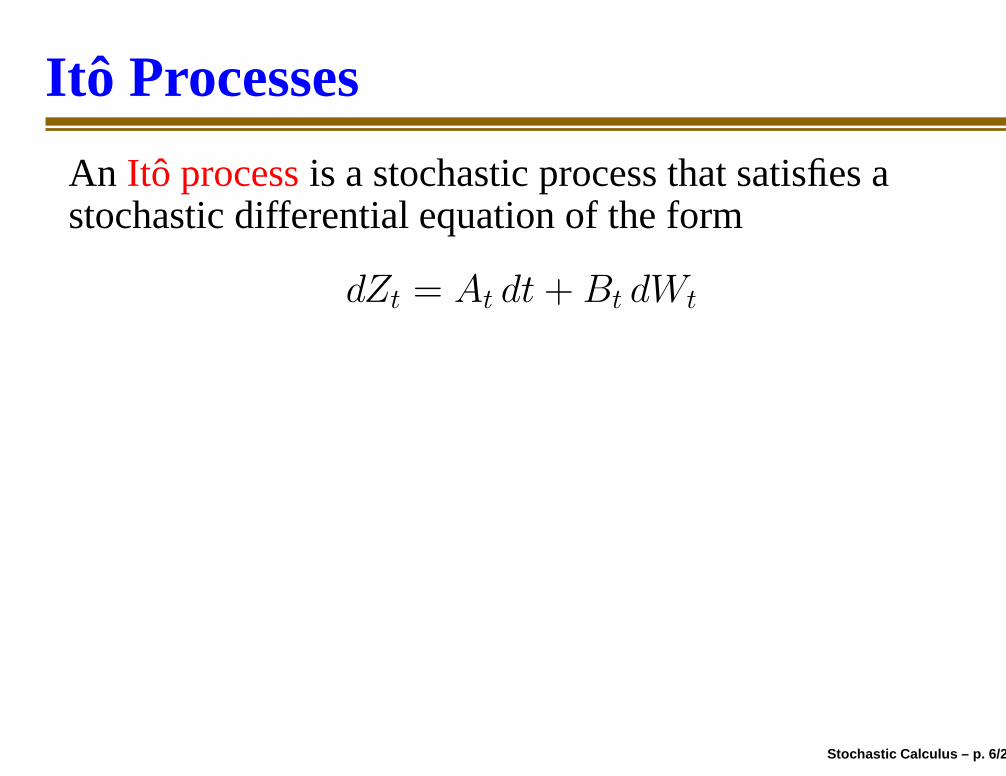
An Itô process is a stochastic process that satisfies astochastic differential equation of the form
dZt = At dt + Bt dWt
Here Wt is a standard Wiener process (Brownianmotion), and At, Bt are adapted process, that is,processes such that for any time t, the current valuesAt, Bt are independent of the future increments of theWiener process.
The local quadratic variation of the Itô process Zt isdefined by
d[Z,Z]t = B2
t dt
Stochastic Calculus – p. 6/27
Itô Processes
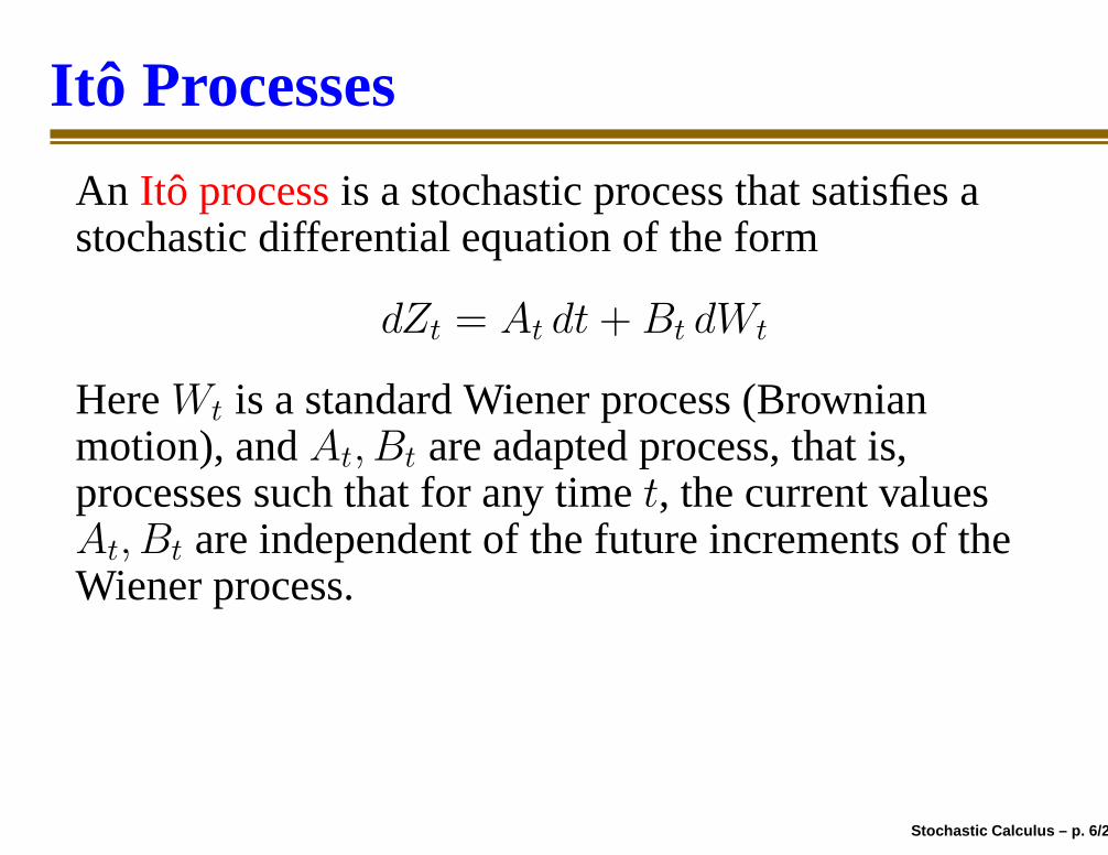
An Itô process is a stochastic process that satisfies astochastic differential equation of the form
dZt = At dt + Bt dWt
Here Wt is a standard Wiener process (Brownianmotion), and At, Bt are adapted process, that is,processes such that for any time t, the current valuesAt, Bt are independent of the future increments of theWiener process.
The local quadratic variation of the Itô process Zt isdefined by
d[Z,Z]t = B2
t dt
Stochastic Calculus – p. 6/27
Itô Processes
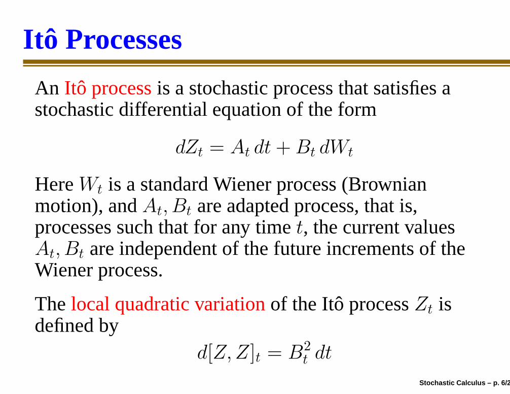
An Itô process is a stochastic process that satisfies astochastic differential equation of the form
dZt = At dt + Bt dWt
Here Wt is a standard Wiener process (Brownianmotion), and At, Bt are adapted process, that is,processes such that for any time t, the current valuesAt, Bt are independent of the future increments of theWiener process.
The local quadratic variation of the Itô process Zt isdefined by
d[Z,Z]t = B2
t dt
Stochastic Calculus – p. 6/27
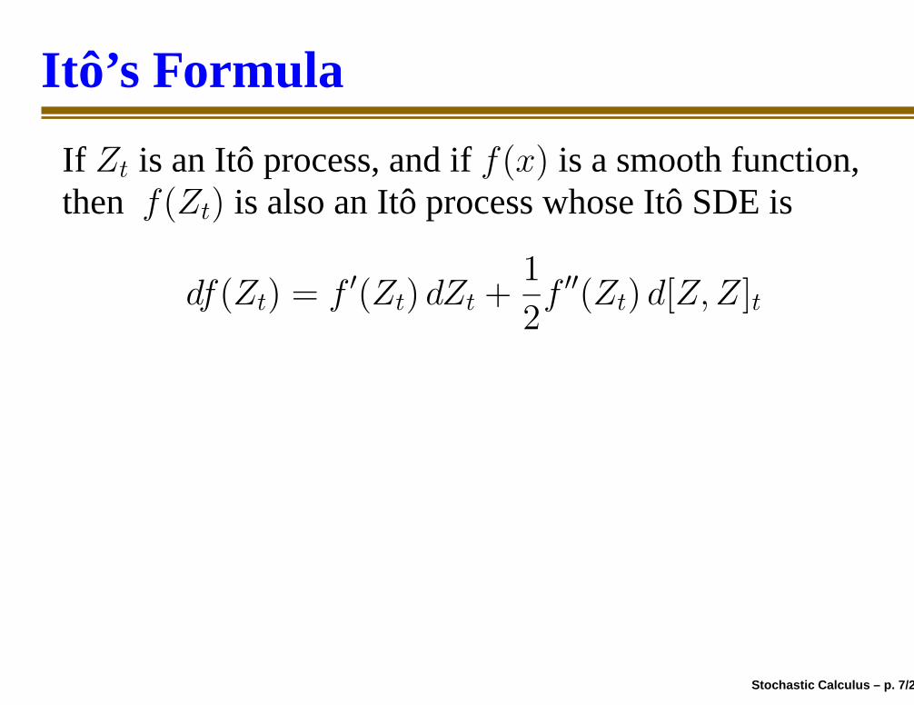
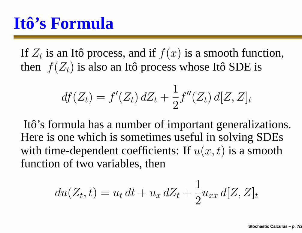
Itô’s Formula
If Zt is an Itô process, and if f(x) is a smooth function,then f(Zt) is also an Itô process whose Itô SDE is
df(Zt) = f ′(Zt) dZt +1
2f ′′(Zt) d[Z,Z]t
Itô’s formula has a number of important generalizations.Here is one which is sometimes useful in solving SDEswith time-dependent coefficients: If u(x, t) is a smoothfunction of two variables, then
du(Zt, t) = ut dt + ux dZt +1
2uxx d[Z,Z]t
Stochastic Calculus – p. 7/27

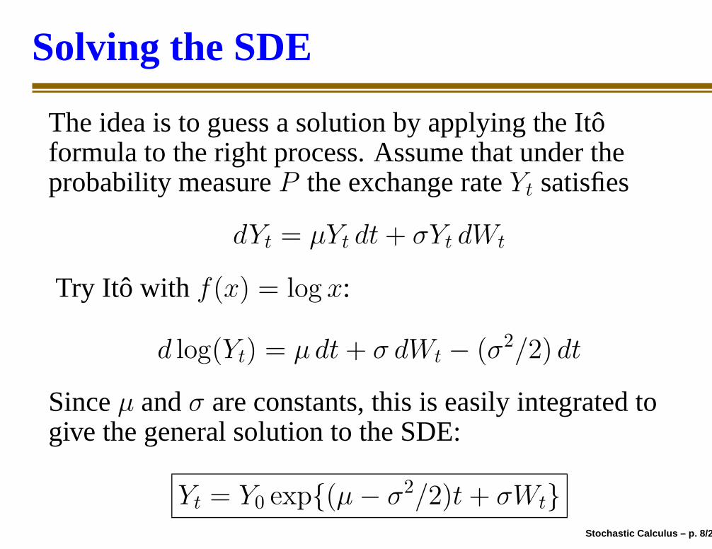
Solving the SDE
The idea is to guess a solution by applying the Itôformula to the right process. Assume that under theprobability measure P the exchange rate Yt satisfies
dYt = µYt dt + σYt dWt
Try Itô with f(x) = log x:
d log(Yt) = µ dt + σ dWt − (σ2/2) dt
Since µ and σ are constants, this is easily integrated togive the general solution to the SDE:
Yt = Y0 exp{(µ− σ2/2)t + σWt}
Stochastic Calculus – p. 8/27
Solving the SDE
The idea is to guess a solution by applying the Itôformula to the right process. Assume that under theprobability measure P the exchange rate Yt satisfies
dYt = µYt dt + σYt dWt
Try Itô with f(x) = log x:
d log(Yt) = µ dt + σ dWt − (σ2/2) dt
Since µ and σ are constants, this is easily integrated togive the general solution to the SDE:
Yt = Y0 exp{(µ− σ2/2)t + σWt}Stochastic Calculus – p. 8/27

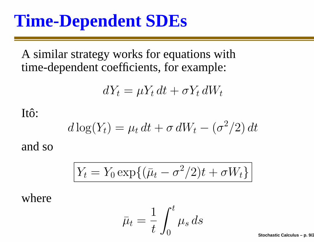
Time-Dependent SDEs
A similar strategy works for equations withtime-dependent coefficients, for example:
dYt = µYt dt + σYt dWt
Itô:d log(Yt) = µt dt + σ dWt − (σ2/2) dt
and so
Yt = Y0 exp{(µ̄t − σ2/2)t + σWt}
where
µ̄t =1
t
∫ t
0
µs ds
Stochastic Calculus – p. 9/27

Time-Dependent SDEs
A similar strategy works for equations withtime-dependent coefficients, for example:
dYt = µYt dt + σYt dWt
Itô:d log(Yt) = µt dt + σ dWt − (σ2/2) dt
and so
Yt = Y0 exp{(µ̄t − σ2/2)t + σWt}
where
µ̄t =1
t
∫ t
0
µs ds
Stochastic Calculus – p. 9/27
Time-Dependent SDEs
A similar strategy works for equations withtime-dependent coefficients, for example:
dYt = µYt dt + σYt dWt
Itô:d log(Yt) = µt dt + σ dWt − (σ2/2) dt
and so
Yt = Y0 exp{(µ̄t − σ2/2)t + σWt}
where
µ̄t =1
t
∫ t
0
µs dsStochastic Calculus – p. 9/27
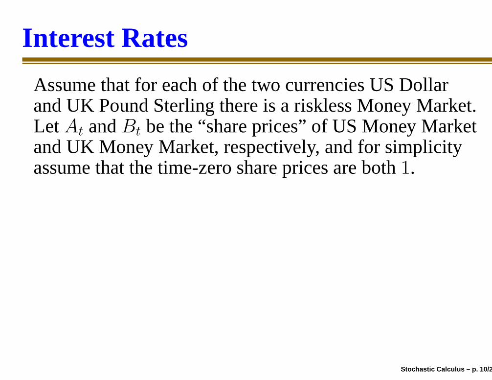
Interest Rates
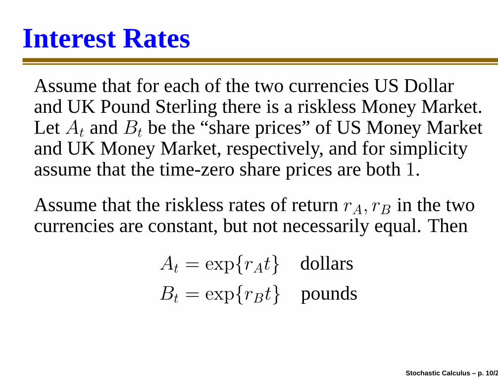
Assume that for each of the two currencies US Dollarand UK Pound Sterling there is a riskless Money Market.Let At and Bt be the “share prices” of US Money Marketand UK Money Market, respectively, and for simplicityassume that the time-zero share prices are both 1.
Assume that the riskless rates of return rA, rB in the twocurrencies are constant, but not necessarily equal. Then
At = exp{rAt} dollars
Bt = exp{rBt} pounds
Stochastic Calculus – p. 10/27
Interest Rates
Assume that for each of the two currencies US Dollarand UK Pound Sterling there is a riskless Money Market.Let At and Bt be the “share prices” of US Money Marketand UK Money Market, respectively, and for simplicityassume that the time-zero share prices are both 1.
Assume that the riskless rates of return rA, rB in the twocurrencies are constant, but not necessarily equal. Then
At = exp{rAt} dollars
Bt = exp{rBt} pounds
Stochastic Calculus – p. 10/27

Exchange and Interest Rates
The asset US Money Market is riskless to a Dollarinvestor, but not to a Pound Sterling investor. Evaluatedin Pounds Sterling, the share price of the US MoneyMarket asset is
AtYt = Y0 exp{rAt + µt− σ2t/2 + σWt}
where Wt is a standard Wiener Process under the riskneutral probability measure QB for Pound investors.
Theorem: µ = rB − rA.
Stochastic Calculus – p. 11/27

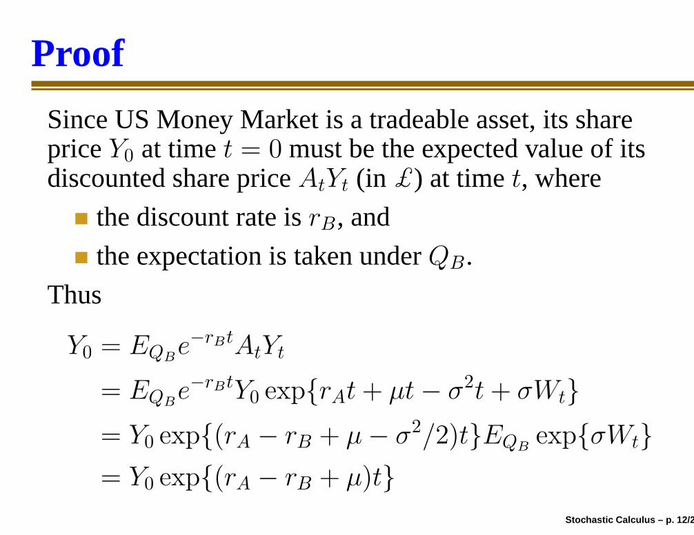
Proof
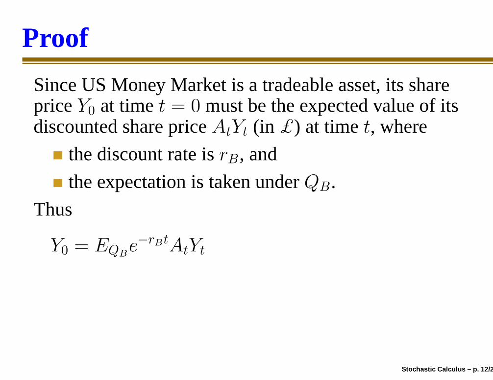
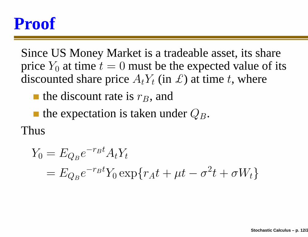
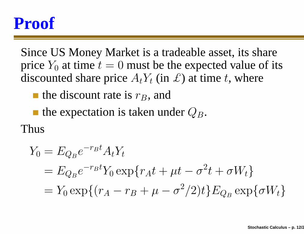
Since US Money Market is a tradeable asset, its shareprice Y0 at time t = 0 must be the expected value of itsdiscounted share price AtYt (in £) at time t, where
the discount rate is rB, and
the expectation is taken under QB.
Thus
Y0 = EQBe−rBtAtYt
= EQBe−rBtY0 exp{rAt + µt− σ2t + σWt}
= Y0 exp{(rA − rB + µ− σ2/2)t}EQBexp{σWt}
= Y0 exp{(rA − rB + µ)t}
Stochastic Calculus – p. 12/27

Proof
Since US Money Market is a tradeable asset, its shareprice Y0 at time t = 0 must be the expected value of itsdiscounted share price AtYt (in £) at time t, where
the discount rate is rB, and
the expectation is taken under QB.
Thus
Y0 = EQBe−rBtAtYt
= EQBe−rBtY0 exp{rAt + µt− σ2t + σWt}
= Y0 exp{(rA − rB + µ− σ2/2)t}EQBexp{σWt}
= Y0 exp{(rA − rB + µ)t}
Stochastic Calculus – p. 12/27

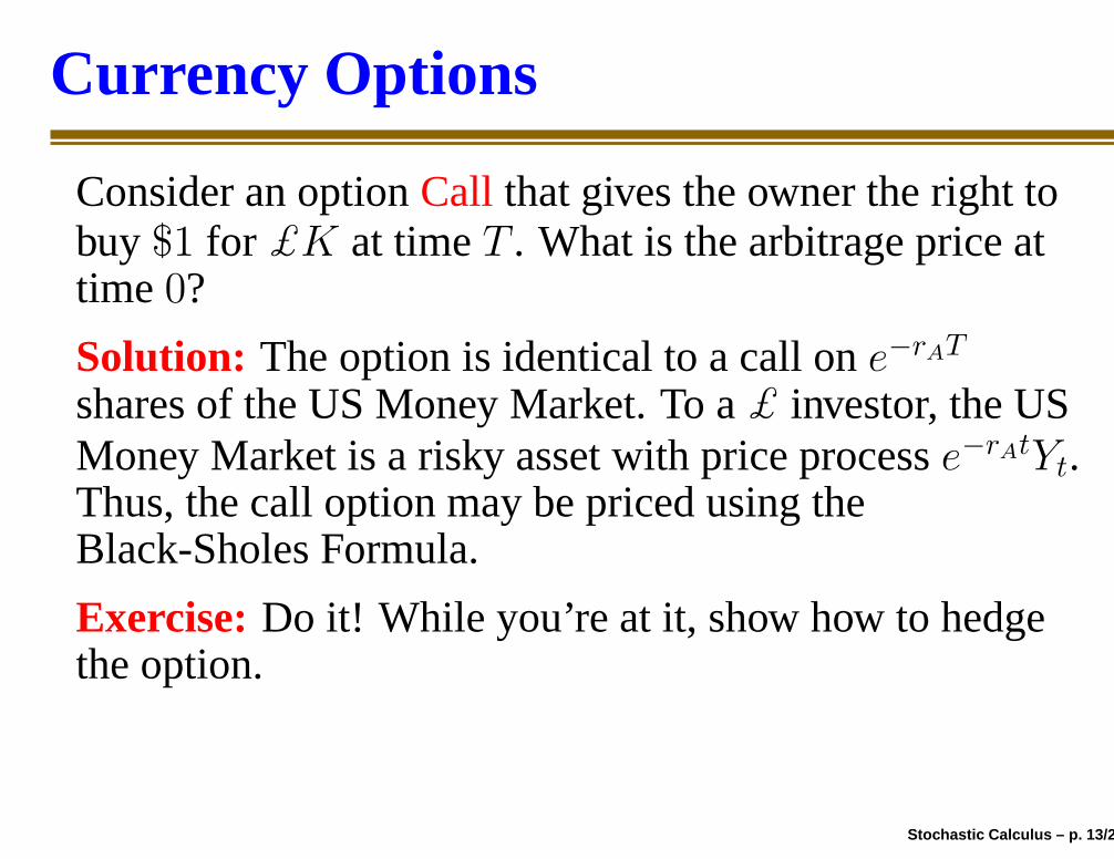
Currency Options
Consider an option Call that gives the owner the right tobuy $1 for £K at time T . What is the arbitrage price attime 0?
Solution: The option is identical to a call on e−rAT
shares of the US Money Market. To a £ investor, the USMoney Market is a risky asset with price process e−rAtYt.Thus, the call option may be priced using theBlack-Sholes Formula.
Exercise: Do it! While you’re at it, show how to hedgethe option.
Stochastic Calculus – p. 13/27

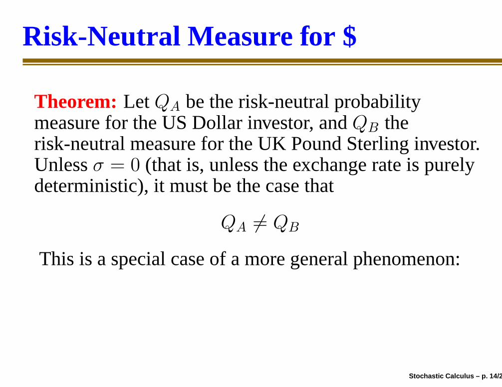
Risk-Neutral Measure for $
Theorem: Let QA be the risk-neutral probabilitymeasure for the US Dollar investor, and QB therisk-neutral measure for the UK Pound Sterling investor.Unless σ = 0 (that is, unless the exchange rate is purelydeterministic), it must be the case that
QA 6= QB
This is a special case of a more general phenomenon:
Stochastic Calculus – p. 14/27
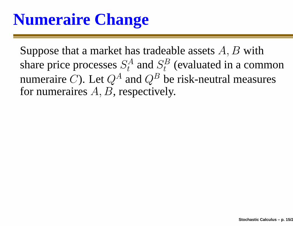
Numeraire Change
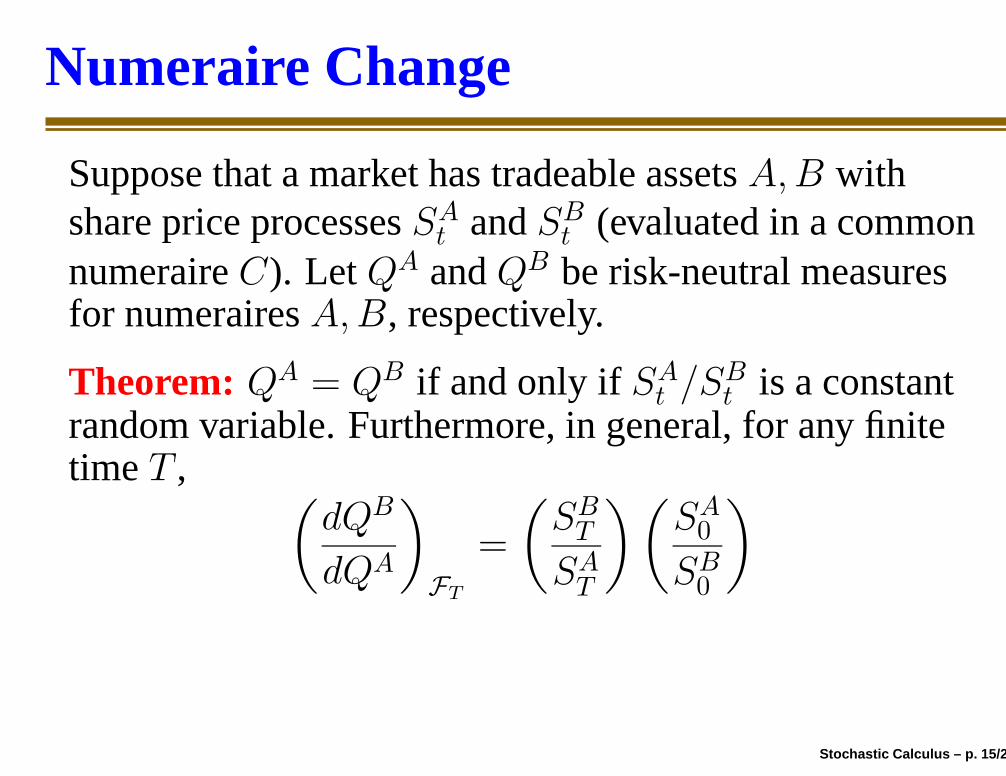
Suppose that a market has tradeable assets A,B withshare price processes SA
t and SBt (evaluated in a common
numeraire C). Let QA and QB be risk-neutral measuresfor numeraires A,B, respectively.
Theorem: QA = QB if and only if SAt /SB
t is a constantrandom variable. Furthermore, in general, for any finitetime T ,
(
dQB
dQA
)
FT
=
(
SBT
SAT
)(
SA0
SB0
)
Stochastic Calculus – p. 15/27
Numeraire Change
Suppose that a market has tradeable assets A,B withshare price processes SA
t and SBt (evaluated in a common
numeraire C). Let QA and QB be risk-neutral measuresfor numeraires A,B, respectively.
Theorem: QA = QB if and only if SAt /SB
t is a constantrandom variable. Furthermore, in general, for any finitetime T ,
(
dQB
dQA
)
FT
=
(
SBT
SAT
)(
SA0
SB0
)
Stochastic Calculus – p. 15/27
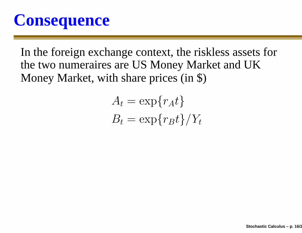
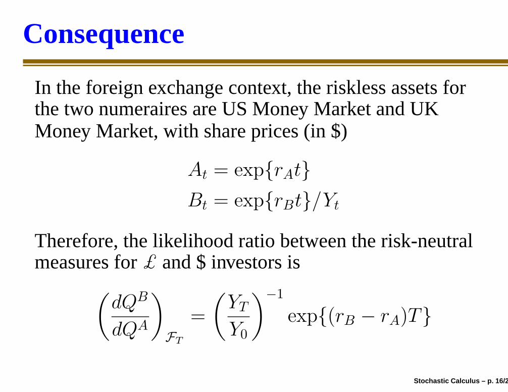
Consequence
In the foreign exchange context, the riskless assets forthe two numeraires are US Money Market and UKMoney Market, with share prices (in $)
At = exp{rAt}
Bt = exp{rBt}/Yt
Therefore, the likelihood ratio between the risk-neutralmeasures for £ and $ investors is
(
dQB
dQA
)
FT
=
(
YT
Y0
)−1
exp{(rB − rA)T}
Stochastic Calculus – p. 16/27

Likelihood Ratio Identity
Let V it be the time-t share price of any contingent claim
in numeraire i = A,B,C. These share prices satisfy:
V At = V C
t /SAt
V Bt = V C
t /SBt
The time-zero share price is the discounted expectedvalue of the time−t share price for each of thenumeraires A,B. The discount factors are 1, so
V A0
= V C0
/SA0
= EAV Ct /SA
t
V B0
= V C0
/SB0
= EBV Ct /SB
t
Stochastic Calculus – p. 17/27

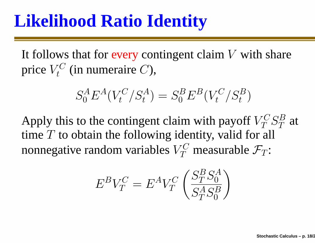
Likelihood Ratio Identity
It follows that for every contingent claim V with shareprice V C
t (in numeraire C),
SA0EA(V C
t /SAt ) = SB
0EB(V C
t /SBt )
Apply this to the contingent claim with payoff V CT SB
T attime T to obtain the following identity, valid for allnonnegative random variables V C
T measurable FT :
EBV CT = EAV C
T
(
SBT SA
0
SAT SB
0
)
This is the defining property of a likelihood ratio.
Stochastic Calculus – p. 18/27
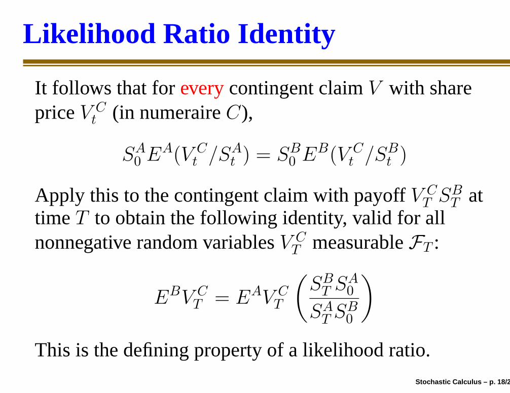
Likelihood Ratio Identity
It follows that for every contingent claim V with shareprice V C
t (in numeraire C),
SA0EA(V C
t /SAt ) = SB
0EB(V C
t /SBt )
Apply this to the contingent claim with payoff V CT SB
T attime T to obtain the following identity, valid for allnonnegative random variables V C
T measurable FT :
EBV CT = EAV C
T
(
SBT SA
0
SAT SB
0
)
This is the defining property of a likelihood ratio.Stochastic Calculus – p. 18/27
Exponential Martingales
Let Wt be a standard Wiener process, wth Brownianfiltration Ft, and let θt be a bounded, adapted process.Define
Zt = exp
{∫ t
0
θs dWs −
∫ t
0
θ2
s ds/2
}
Fact: Zt is a positive martingale. Proof: Itô!
dZt = Ztθt dWt − Ztθ2
t dt/2+Ztθ2
t dt/2
= Ztθt dWt =⇒
Zt = Z0 +
∫ t
0
Zsθs dWs
Stochastic Calculus – p. 19/27
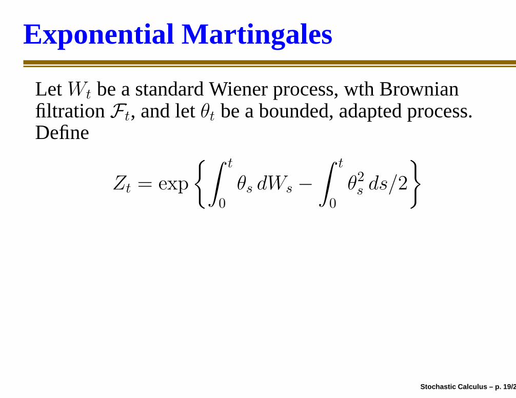
Exponential Martingales
Let Wt be a standard Wiener process, wth Brownianfiltration Ft, and let θt be a bounded, adapted process.Define
Zt = exp
{∫ t
0
θs dWs −
∫ t
0
θ2
s ds/2
}
Fact: Zt is a positive martingale.
Proof: Itô!
dZt = Ztθt dWt − Ztθ2
t dt/2+Ztθ2
t dt/2
= Ztθt dWt =⇒
Zt = Z0 +
∫ t
0
Zsθs dWs
Stochastic Calculus – p. 19/27

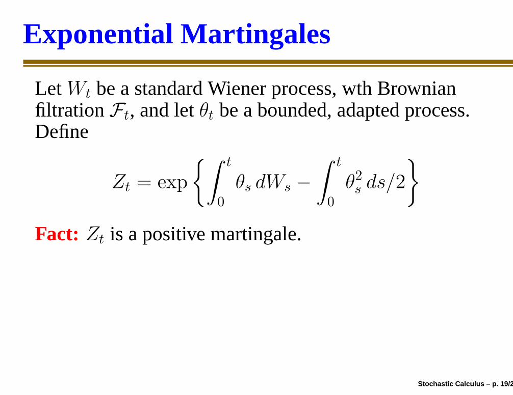
Exponential Martingales
Let Wt be a standard Wiener process, wth Brownianfiltration Ft, and let θt be a bounded, adapted process.Define
Zt = exp
{∫ t
0
θs dWs −
∫ t
0
θ2
s ds/2
}
Fact: Zt is a positive martingale. Proof: Itô!
dZt = Ztθt dWt − Ztθ2
t dt/2+Ztθ2
t dt/2
= Ztθt dWt =⇒
Zt = Z0 +
∫ t
0
Zsθs dWs
Stochastic Calculus – p. 19/27

Exponential Martingales
Let Wt be a standard Wiener process, wth Brownianfiltration Ft, and let θt be a bounded, adapted process.Define
Zt = exp
{∫ t
0
θs dWs −
∫ t
0
θ2
s ds/2
}
Fact: Zt is a positive martingale. Proof: Itô!
dZt = Ztθt dWt − Ztθ2
t dt/2+Ztθ2
t dt/2
= Ztθt dWt =⇒
Zt = Z0 +
∫ t
0
Zsθs dWs
Stochastic Calculus – p. 19/27
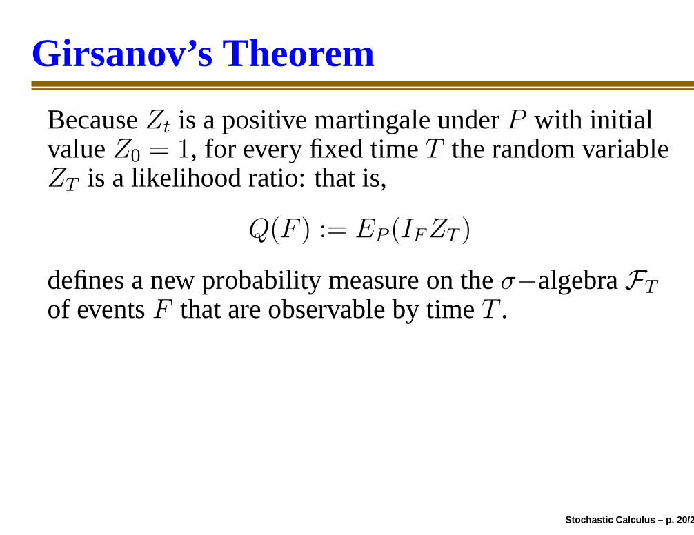
Girsanov’s Theorem
Because Zt is a positive martingale under P with initialvalue Z0 = 1, for every fixed time T the random variableZT is a likelihood ratio: that is,
Q(F ) := EP (IFZT )
defines a new probability measure on the σ−algebra FT
of events F that are observable by time T .
Theorem: Under the measure Q, the process{Wt −
∫ t
0θsds}0≤t≤T is a standard Wiener process.
Stochastic Calculus – p. 20/27
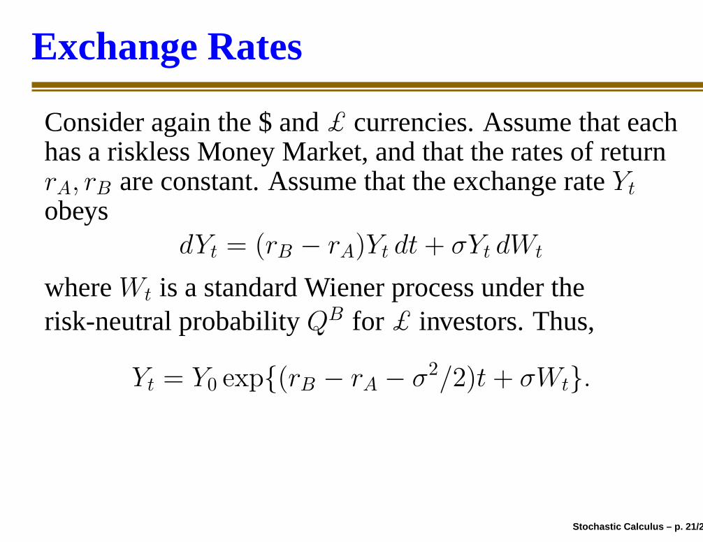
Exchange Rates
Consider again the $ and £ currencies. Assume that eachhas a riskless Money Market, and that the rates of returnrA, rB are constant. Assume that the exchange rate Yt
obeysdYt = (rB − rA)Yt dt + σYt dWt
where Wt is a standard Wiener process under therisk-neutral probability QB for £ investors. Thus,
Yt = Y0 exp{(rB − rA − σ2/2)t + σWt}.
Stochastic Calculus – p. 21/27
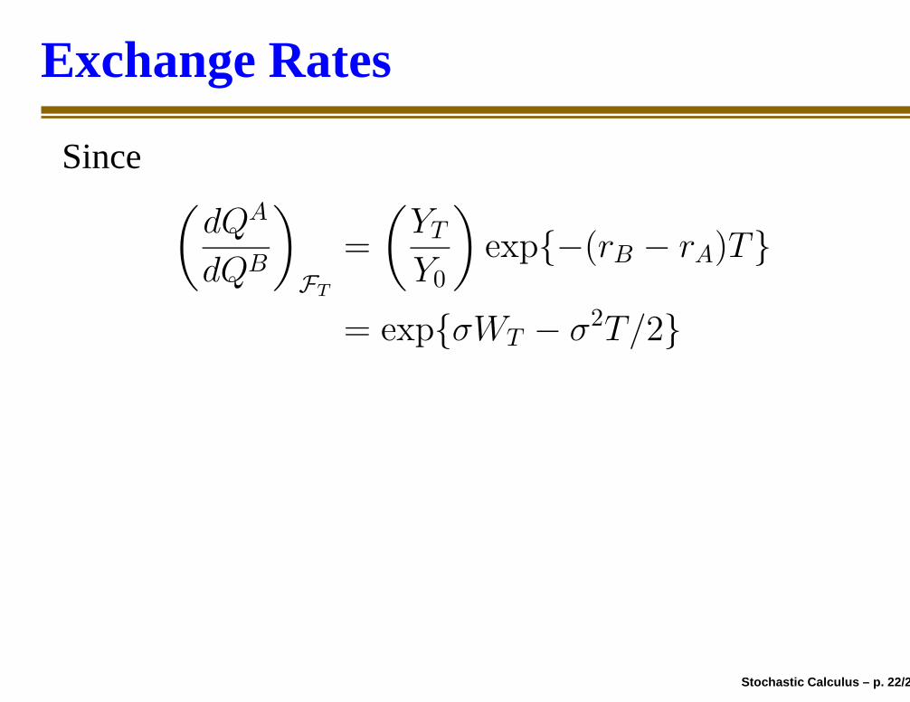
Exchange Rates
Since(
dQA
dQB
)
FT
=
(
YT
Y0
)
exp{−(rB − rA)T}
= exp{σWT − σ2T/2}
Girsanov implies that under QA the process Wt is aWiener process with drift σ. Thus, to the $ investor, itappears that the exchange rate obeys
dYt = (rB − rA − σ2)Yt dt + σYt dW̃t
where W̃t is a standard Wiener process under QA.
Stochastic Calculus – p. 22/27

Exchange Rates
Since(
dQA
dQB
)
FT
=
(
YT
Y0
)
exp{−(rB − rA)T}
= exp{σWT − σ2T/2}
Girsanov implies that under QA the process Wt is aWiener process with drift σ. Thus, to the $ investor, itappears that the exchange rate obeys
dYt = (rB − rA − σ2)Yt dt + σYt dW̃t
where W̃t is a standard Wiener process under QA.Stochastic Calculus – p. 22/27

Stochastic Calculus – p. 23/27

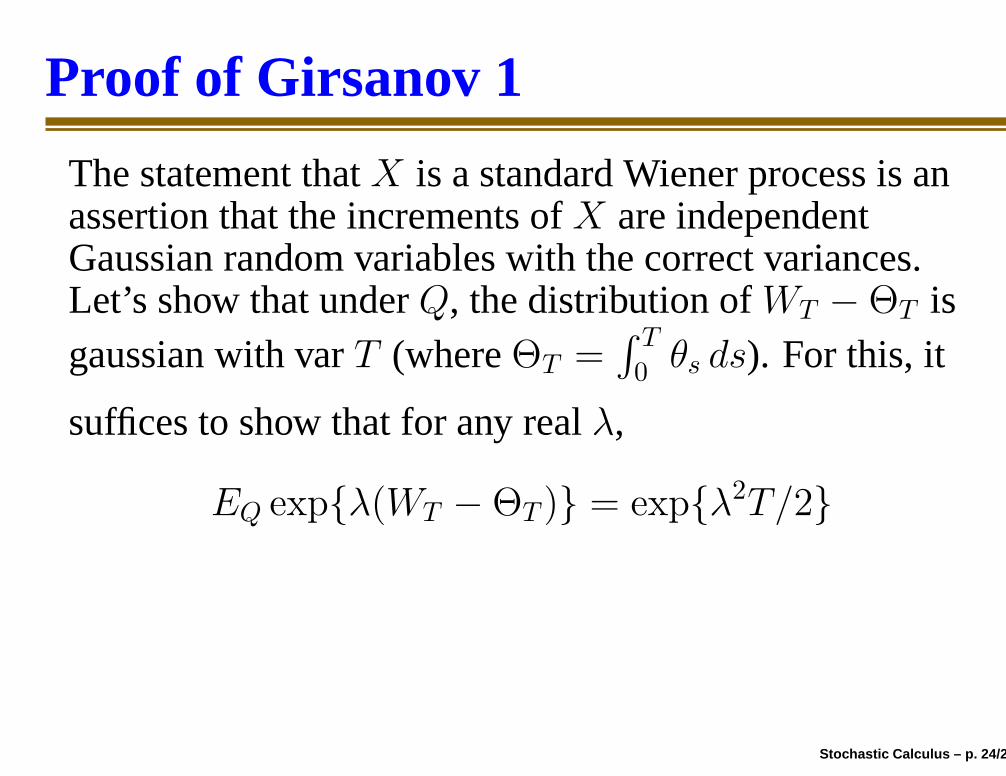
Proof of Girsanov 1
The statement that X is a standard Wiener process is anassertion that the increments of X are independentGaussian random variables with the correct variances.Let’s show that under Q, the distribution of WT −ΘT isgaussian with var T (where ΘT =
∫ T
0θs ds).
For this, it
suffices to show that for any real λ,
EQ exp{λ(WT −ΘT )} = exp{λ2T/2}
To evaluate the expectation, change measure:
EQ exp{λ(WT −ΘT )} = EP exp{λ(WT −ΘT )}ZT
Stochastic Calculus – p. 24/27
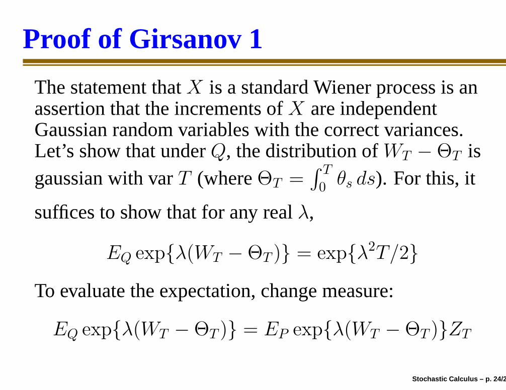
Proof of Girsanov 1
The statement that X is a standard Wiener process is anassertion that the increments of X are independentGaussian random variables with the correct variances.Let’s show that under Q, the distribution of WT −ΘT isgaussian with var T (where ΘT =
∫ T
0θs ds). For this, it
suffices to show that for any real λ,
EQ exp{λ(WT −ΘT )} = exp{λ2T/2}
To evaluate the expectation, change measure:
EQ exp{λ(WT −ΘT )} = EP exp{λ(WT −ΘT )}ZT
Stochastic Calculus – p. 24/27

Proof of Girsanov 2
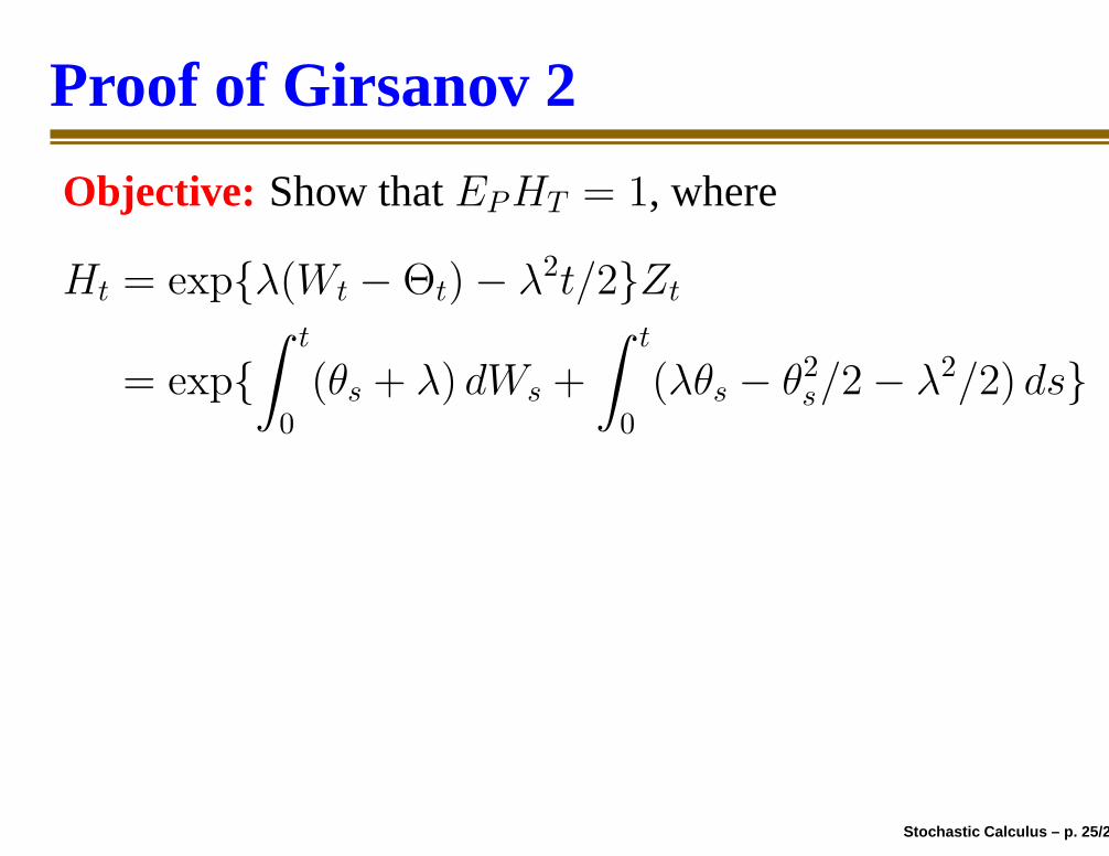
Objective: Show that EPHT = 1, where
Ht = exp{λ(Wt −Θt)− λ2t/2}Zt
= exp{
∫ t
0
(θs + λ) dWs +
∫ t
0
(λθs − θ2
s/2− λ2/2) ds}
= exp{
∫ t
0
(θs + λ) dWs −
∫ t
0
(θs + λ)2 ds/2}
Thus, Ht is an exponential martingale under P , and so itsexpectation is constant over time. A similar calculationestablishes the independence of the increments.
Stochastic Calculus – p. 25/27
Proof of Girsanov 2
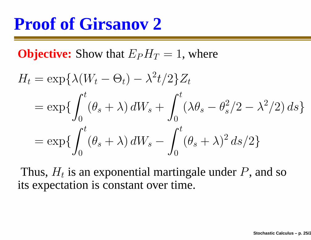
Objective: Show that EPHT = 1, where
Ht = exp{λ(Wt −Θt)− λ2t/2}Zt
= exp{
∫ t
0
(θs + λ) dWs +
∫ t
0
(λθs − θ2
s/2− λ2/2) ds}
= exp{
∫ t
0
(θs + λ) dWs −
∫ t
0
(θs + λ)2 ds/2}
Thus, Ht is an exponential martingale under P , and so itsexpectation is constant over time. A similar calculationestablishes the independence of the increments.
Stochastic Calculus – p. 25/27

Proof of Girsanov 2
Objective: Show that EPHT = 1, where
Ht = exp{λ(Wt −Θt)− λ2t/2}Zt
= exp{
∫ t
0
(θs + λ) dWs +
∫ t
0
(λθs − θ2
s/2− λ2/2) ds}
= exp{
∫ t
0
(θs + λ) dWs −
∫ t
0
(θs + λ)2 ds/2}
Thus, Ht is an exponential martingale under P , and so itsexpectation is constant over time. A similar calculationestablishes the independence of the increments.
Stochastic Calculus – p. 25/27
Proof of Girsanov 2
Objective: Show that EPHT = 1, where
Ht = exp{λ(Wt −Θt)− λ2t/2}Zt
= exp{
∫ t
0
(θs + λ) dWs +
∫ t
0
(λθs − θ2
s/2− λ2/2) ds}
= exp{
∫ t
0
(θs + λ) dWs −
∫ t
0
(θs + λ)2 ds/2}
Thus, Ht is an exponential martingale under P , and soits expectation is constant over time.
A similarcalculation establishes the independence of theincrements.
Stochastic Calculus – p. 25/27
Proof of Girsanov 2
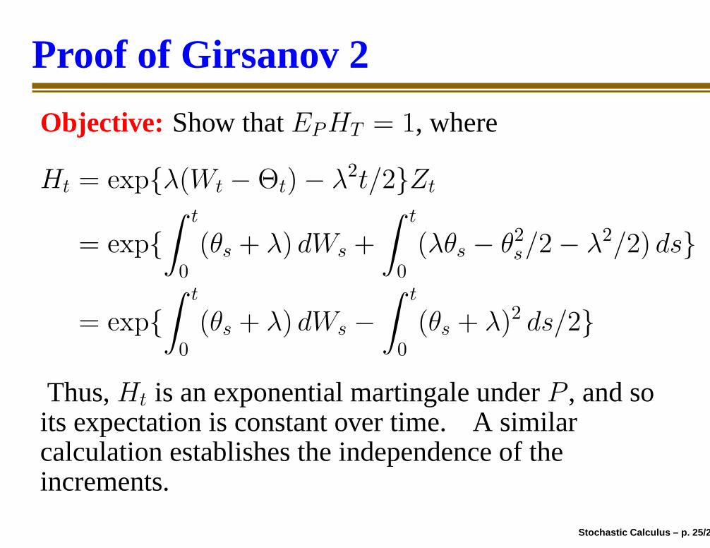
Objective: Show that EPHT = 1, where
Ht = exp{λ(Wt −Θt)− λ2t/2}Zt
= exp{
∫ t
0
(θs + λ) dWs +
∫ t
0
(λθs − θ2
s/2− λ2/2) ds}
= exp{
∫ t
0
(θs + λ) dWs −
∫ t
0
(θs + λ)2 ds/2}
Thus, Ht is an exponential martingale under P , and soits expectation is constant over time. A similarcalculation establishes the independence of theincrements.
Stochastic Calculus – p. 25/27

Scratch
Stochastic Calculus – p. 26/27

Scratch
Stochastic Calculus – p. 26/27

Scratch
Stochastic Calculus – p. 26/27

Scratch
Stochastic Calculus – p. 27/27

Scratch
Stochastic Calculus – p. 27/27

Scratch
Stochastic Calculus – p. 27/27


![Itô and Stratonovich Stochastic Calculus€¦ · We provide a detailed hands-on tutorial for the R Development Core Team[2014] add-on package Sim.DiffProc [Guidoum and Boukhetala,2014],](https://static.documents.pub/doc/80x56/5b0d98127f8b9ab7658ca2c4/it-and-stratonovich-stochastic-calculus-provide-a-detailed-hands-on-tutorial-for.jpg)


