STOCHASTIC MODELING OF HIGH-LEVEL STRUCTURES IN ...

STOCHASTIC MODELING OF HIGH-LEVELSTRUCTURES IN HANDWRITTEN WORD

RECOGNITION

By

Hanhong Xue

May 2002

A DISSERTATION SUBMITTED TO THE

FACULTY OF THE GRADUATE SCHOOL OF STATE

UNIVERSITY OF NEW YORK AT BUFFALO

IN PARTIAL FULFILLMENT OF THE REQUIREMENTS

FOR THE DEGREE OF

DOCTOR OF PHILOSOPHY

c�

Hanhong Xue, 2002

All Rights Reserved

To My Parents

and

My Wife

ACKNOWLEDGMENTS

I would like to express my deep appreciation to Dr. Venu Govindaraju, my advisor and

chair of my dissertation committee, for his persistent guidance and valuable advice on this

research. He led me to the frontier of handwriting recognition and encouraged me to tackle

challenging problems in this field. Without him, this dissertation would never have been

possible.

I am also grateful to Dr. Bharat Jayaraman, member of my dissertation committee, for

his full support to my graduate studies and early discussions on stochastic grammars which

later turned out to be the theoretical basis of this research.

I would also like to show my gratitude to Dr. Peter Scott, member of my dissertation

committee. His professional experience in pattern recognition has helped me much in

developing some major research topics in this work and his lecture on Machine Learning

introduced me a solid foundation of this research.

Special thanks go to Dr. John Pitrelli in IBM T.J. Watson Research Center. As the out-

side reader of my dissertation, he thoroughly reviewed my manuscript with his expertise in

handwriting recognition. His many insightful suggestions have helped improve the overall

quality of my dissertation significantly.

I would also like to give my thanks to the Center of Excellence for Document Analysis

and Recognition (CEDAR), under the enthusiastic leadership of Dr. Sargur N. Srihari and

Dr. Venu Govindaraju, for providing me an ideal research environment. I would especially

like to thank Bruce Specht, Kristen Pfaff, and Eugenia Smith, for their kindly administrative

support to my research work and my defense.

Thanks to former/current research scientists in CEDAR. They are Dr. Djamel Bouchaf-

fra, for introducing hidden Markov modeling to me, Dr. Jaehwa Park, Dr. Petr Slavik, Dr.

Aibing Rao, Sergey Tulyakov and Ankur M. Teredesai, for discussions on my work and

their suggestions.

ABSTRACT

Handwritten word recognition is an important topic in pattern recognition. It has

many applications in automated document processing such as postal address interpreta-

tion, bankcheck reading and form reading. There is evidence from psychological studies

that word shape plays a significant role in human visual word recognition. High-level struc-

tures in handwriting, such as loops, junctions, turns, and ends, are considered to be highly

shape-defining. These structures can be more precisely described by their attributes such as

position, orientation, curvature, and size. Algorithms based on skeletal graphs are designed

to extract structural features. Viewing handwriting as a sequence of structural features, we

choose stochastic finite-state automata (SFSAs) as our modeling tool. We extend SFSAs

to model high-level structures and their continuous attributes, and view the popular hidden

Markov models (HMMs) as special cases of SFSAs obtained by tying parameters on transi-

tions. Experimental results on these two modeling tools have shown advantages of SFSAs

over HMMs. To allow real-time applications of the stochastic word recognizers, we in-

troduce several fast-decoding techniques, including character-level dynamic programming,

duration constraint, prefix/suffix sharing, choice pruning, etc. A parallel version of the rec-

ognizer is also implemented by splitting large lexicons. The resulting word recognizer is

better than or comparable to other recognizers in terms of recognition accuracy and speed.

For recognizers building word recognition on character recognition, we propose a perfor-

mance model to associate word recognition accuracy with character recognition accuracy.

The model parameters can be determined by multiple regression on accuracy rates obtained

on the training data. This model can be used to predict a recognizer’s performance given a

lexicon and promises its applications in dynamic classifier selection and combination.

Contents

1 Introduction 1

1.1 Background . . . . . . . . . . . . . . . . . . . . . . . . . . . . . . . . . . 1

1.2 Problem Definition . . . . . . . . . . . . . . . . . . . . . . . . . . . . . . 2

1.3 Related Work . . . . . . . . . . . . . . . . . . . . . . . . . . . . . . . . . 3

1.4 Motivations . . . . . . . . . . . . . . . . . . . . . . . . . . . . . . . . . . 5

1.5 Proposed Approach . . . . . . . . . . . . . . . . . . . . . . . . . . . . . . 7

1.5.1 Feature extraction . . . . . . . . . . . . . . . . . . . . . . . . . . . 8

1.5.2 Modeling tool . . . . . . . . . . . . . . . . . . . . . . . . . . . . . 8

1.5.3 Modeling characters and words . . . . . . . . . . . . . . . . . . . 10

1.5.4 Fast decoding . . . . . . . . . . . . . . . . . . . . . . . . . . . . . 11

1.5.5 Performance evaluation . . . . . . . . . . . . . . . . . . . . . . . . 12

1.6 Dissertation Outline . . . . . . . . . . . . . . . . . . . . . . . . . . . . . . 13

2 Stochastic Modeling 14

2.1 Introduction . . . . . . . . . . . . . . . . . . . . . . . . . . . . . . . . . . 14

2.2 Problem Definition . . . . . . . . . . . . . . . . . . . . . . . . . . . . . . 15

2.2.1 Observations . . . . . . . . . . . . . . . . . . . . . . . . . . . . . 15

2.2.2 Stochastic training . . . . . . . . . . . . . . . . . . . . . . . . . . 16

2.2.3 Stochastic decoding . . . . . . . . . . . . . . . . . . . . . . . . . 19

i

2.3 Finite-State Automata . . . . . . . . . . . . . . . . . . . . . . . . . . . . . 20

2.4 Discrete Stochastic Finite-State Automata . . . . . . . . . . . . . . . . . . 21

2.4.1 Definition . . . . . . . . . . . . . . . . . . . . . . . . . . . . . . . 22

2.4.2 Training . . . . . . . . . . . . . . . . . . . . . . . . . . . . . . . . 24

2.4.3 Decoding . . . . . . . . . . . . . . . . . . . . . . . . . . . . . . . 30

2.4.4 Complexity analysis . . . . . . . . . . . . . . . . . . . . . . . . . 32

2.5 Hidden Markov Models . . . . . . . . . . . . . . . . . . . . . . . . . . . . 33

2.5.1 Viewing HMMs as special SFSAs . . . . . . . . . . . . . . . . . . 34

2.5.2 Definition . . . . . . . . . . . . . . . . . . . . . . . . . . . . . . . 36

2.5.3 Training . . . . . . . . . . . . . . . . . . . . . . . . . . . . . . . . 37

2.5.4 Decoding . . . . . . . . . . . . . . . . . . . . . . . . . . . . . . . 38


2.6 Conclusions . . . . . . . . . . . . . . . . . . . . . . . . . . . . . . . . . . 39

3 Extraction of Structural Features 40

3.1 Introduction . . . . . . . . . . . . . . . . . . . . . . . . . . . . . . . . . . 40

3.1.1 High-level structural features . . . . . . . . . . . . . . . . . . . . . 41

3.1.2 Feature extraction outline . . . . . . . . . . . . . . . . . . . . . . 43

3.2 Preprocessing . . . . . . . . . . . . . . . . . . . . . . . . . . . . . . . . . 44

3.2.1 Smoothing . . . . . . . . . . . . . . . . . . . . . . . . . . . . . . 44

3.2.2 Baseline detection . . . . . . . . . . . . . . . . . . . . . . . . . . 46

3.2.3 Slant detection . . . . . . . . . . . . . . . . . . . . . . . . . . . . 47

3.2.4 Compound skew-slant correction . . . . . . . . . . . . . . . . . . . 49

3.2.5 Average stroke width . . . . . . . . . . . . . . . . . . . . . . . . . 49

3.3 Building Block Adjacency Graphs . . . . . . . . . . . . . . . . . . . . . . 50

3.3.1 Stroke mending . . . . . . . . . . . . . . . . . . . . . . . . . . . . 52

3.4 Building Skeletal Graphs . . . . . . . . . . . . . . . . . . . . . . . . . . . 52

ii

3.5 Structural Feature Extraction . . . . . . . . . . . . . . . . . . . . . . . . . 55

3.6 Outer Contour Traveling and Feature Ordering . . . . . . . . . . . . . . . . 56

3.7 Experiments . . . . . . . . . . . . . . . . . . . . . . . . . . . . . . . . . . 58

3.8 Conclusions . . . . . . . . . . . . . . . . . . . . . . . . . . . . . . . . . . 59

4 Modeling Handwritten Words 61

4.1 Introduction . . . . . . . . . . . . . . . . . . . . . . . . . . . . . . . . . . 61

4.2 Structural Features . . . . . . . . . . . . . . . . . . . . . . . . . . . . . . 63

4.3 Continuous SFSAs for Word Modeling . . . . . . . . . . . . . . . . . . . . 65

4.3.1 Definition . . . . . . . . . . . . . . . . . . . . . . . . . . . . . . . 65

4.3.2 Training . . . . . . . . . . . . . . . . . . . . . . . . . . . . . . . . 67

4.3.3 Decoding . . . . . . . . . . . . . . . . . . . . . . . . . . . . . . . 70

4.4 Continuous HMMs for Word Modeling . . . . . . . . . . . . . . . . . . . 71

4.4.1 Definition . . . . . . . . . . . . . . . . . . . . . . . . . . . . . . . 71

4.4.2 Training . . . . . . . . . . . . . . . . . . . . . . . . . . . . . . . . 73

4.4.3 Decoding . . . . . . . . . . . . . . . . . . . . . . . . . . . . . . . 75

4.5 Modeling words . . . . . . . . . . . . . . . . . . . . . . . . . . . . . . . . 75

4.5.1 Modeling words for training . . . . . . . . . . . . . . . . . . . . . 75

4.5.2 Modeling words for decoding . . . . . . . . . . . . . . . . . . . . 76

4.6 Experimental Results . . . . . . . . . . . . . . . . . . . . . . . . . . . . . 77

4.6.1 The system . . . . . . . . . . . . . . . . . . . . . . . . . . . . . . 77

4.6.2 Effect of continuous attributes . . . . . . . . . . . . . . . . . . . . 80

4.6.3 Comparison between SFSAs and HMMs . . . . . . . . . . . . . . 82

4.6.4 Comparison to other recognizers . . . . . . . . . . . . . . . . . . . 82

4.7 Conclusions . . . . . . . . . . . . . . . . . . . . . . . . . . . . . . . . . . 85

5 Fast Decoding 86

iii

5.1 Introduction . . . . . . . . . . . . . . . . . . . . . . . . . . . . . . . . . . 86

5.2 Related Work . . . . . . . . . . . . . . . . . . . . . . . . . . . . . . . . . 87

5.3 Character-level Dynamic Programming . . . . . . . . . . . . . . . . . . . 91

5.3.1 Fragment probabilities . . . . . . . . . . . . . . . . . . . . . . . . 91

5.3.2 Cutting model topology . . . . . . . . . . . . . . . . . . . . . . . 92

5.3.3 Character-level dynamic programming . . . . . . . . . . . . . . . . 93

5.3.4 The Viterbi version . . . . . . . . . . . . . . . . . . . . . . . . . . 95


5.3.6 Generalization to bi-gram connected word models . . . . . . . . . 98

5.4 Other Speed-Improving Techniques . . . . . . . . . . . . . . . . . . . . . 99

5.4.1 Substring-level dynamic programming . . . . . . . . . . . . . . . . 100

5.4.2 Duration constraint . . . . . . . . . . . . . . . . . . . . . . . . . . 101

5.4.3 Choice pruning . . . . . . . . . . . . . . . . . . . . . . . . . . . . 101

5.4.4 Probability to distance conversion . . . . . . . . . . . . . . . . . . 103

5.4.5 Parallel decoding . . . . . . . . . . . . . . . . . . . . . . . . . . . 104

5.5 Experimental Results . . . . . . . . . . . . . . . . . . . . . . . . . . . . . 105

5.5.1 The system . . . . . . . . . . . . . . . . . . . . . . . . . . . . . . 105

5.5.2 Serial implementation . . . . . . . . . . . . . . . . . . . . . . . . 106

5.5.3 Parallel implementation . . . . . . . . . . . . . . . . . . . . . . . 108

5.6 Conclusions . . . . . . . . . . . . . . . . . . . . . . . . . . . . . . . . . . 110

6 Performance Evaluation 111

6.1 Introduction . . . . . . . . . . . . . . . . . . . . . . . . . . . . . . . . . . 111

6.2 The Performance Model . . . . . . . . . . . . . . . . . . . . . . . . . . . 115

6.2.1 Performance factors . . . . . . . . . . . . . . . . . . . . . . . . . 115

6.2.2 Word model abstraction . . . . . . . . . . . . . . . . . . . . . . . 117

6.2.3 Performance model derivation . . . . . . . . . . . . . . . . . . . . 119

iv

6.3 Experiments . . . . . . . . . . . . . . . . . . . . . . . . . . . . . . . . . . 126

6.3.1 Recognizers . . . . . . . . . . . . . . . . . . . . . . . . . . . . . . 126

6.3.2 Image set . . . . . . . . . . . . . . . . . . . . . . . . . . . . . . . 127

6.3.3 Lexicon generation . . . . . . . . . . . . . . . . . . . . . . . . . . 127

6.3.4 Determining model parameters . . . . . . . . . . . . . . . . . . . . 129

6.3.5 Model verification . . . . . . . . . . . . . . . . . . . . . . . . . . 133

6.4 Classifier Combination . . . . . . . . . . . . . . . . . . . . . . . . . . . . 135

6.5 Discussions . . . . . . . . . . . . . . . . . . . . . . . . . . . . . . . . . . 137

6.5.1 Comparison of recognizers . . . . . . . . . . . . . . . . . . . . . . 137

6.5.2 Influence of word length . . . . . . . . . . . . . . . . . . . . . . . 138

6.5.3 Using other distance measures . . . . . . . . . . . . . . . . . . . . 140

6.6 Conclusions . . . . . . . . . . . . . . . . . . . . . . . . . . . . . . . . . . 141

7 Conclusions 144

7.1 Summary . . . . . . . . . . . . . . . . . . . . . . . . . . . . . . . . . . . 144

7.2 Contributions . . . . . . . . . . . . . . . . . . . . . . . . . . . . . . . . . 146

7.3 Future Directions . . . . . . . . . . . . . . . . . . . . . . . . . . . . . . . 147

7.3.1 Feature extraction . . . . . . . . . . . . . . . . . . . . . . . . . . . 147

7.3.2 Comparison of different modeling frameworks . . . . . . . . . . . 148

7.3.3 Optimizing model topology . . . . . . . . . . . . . . . . . . . . . 149

7.3.4 Performance evaluation . . . . . . . . . . . . . . . . . . . . . . . . 149

v

List of Figures

1.4.1 A graph representation of handwriting for structural feature extraction. (a)

Original image. (b) Skeletal graph. . . . . . . . . . . . . . . . . . . . . . . 7

2.3.1 Examples of deterministic and non-deterministic FSAs, both modeling reg-

ular language � a � b �� abb. . . . . . . . . . . . . . . . . . . . . . . . . . . . 20

2.4.1 Transitions in the context of handwriting recognition, where structural fea-

tures like cross, loop, cusp and circle are used in modeling. . . . . . . . . . 23

2.4.2 Calculation of forward and backward probabilities for stochastic finite-state

automata. Time does not change if the null (ε) symbol is observed and time

increases by 1 if a non-null symbol is observed. . . . . . . . . . . . . . . . 27

2.4.3 The probability of taking a transition from state i to state j observing either

null or ot , given the model λ. . . . . . . . . . . . . . . . . . . . . . . . . . 29

2.4.4 Deciding the best state sequence for an input, hence producing the best

segmentation of the input. . . . . . . . . . . . . . . . . . . . . . . . . . . . 31

2.5.1 An example of HMM in the context of handwriting recognition. . . . . . . 34

vi

2.5.2 Converting a stochastic finite-state automaton (SFSA) to a hidden Markov

model (HMM) by parameter tying. (a) The original SFSA. (b) The view of

observation probabilities as transition probabilities times emission proba-

bilities for SFSA . (c) HMM obtained by tying emission probabilities from

state 1 to state 3 and those from state 2 to state 3. (d) Equivalent SFSA

converted from HMM. (e) The calculation of tied emission probabilities for

state 3. (f) Probabilities of generating some strings by the original SFSA

and the HMM. . . . . . . . . . . . . . . . . . . . . . . . . . . . . . . . . . 35

3.1.1 High-level structural features and their possible continuous attributes . . . . 42

3.1.2 Flow-chart for the entire feature extraction process . . . . . . . . . . . . . 45

3.2.1 Run-level smoothing . . . . . . . . . . . . . . . . . . . . . . . . . . . . . 46

3.2.2 Slant detection on the contour . . . . . . . . . . . . . . . . . . . . . . . . 48

3.2.3 Examples of baseline detection and slant detection . . . . . . . . . . . . . 48

3.3.1 Building block adjacency graphs. The input image is represented in (a)

pixels, (b) horizontal runs, (c) blocks and (d) graph. . . . . . . . . . . . . . 51

3.3.2 Building block adjacency graph. (a) Horizontal runs fail to capture the

cross structure while (b) Diagonal runs succeed. . . . . . . . . . . . . . . 51

3.3.3 Stroke mending . . . . . . . . . . . . . . . . . . . . . . . . . . . . . . . . 52

3.4.1 Graph representation of images. (a) input image, (b) initial BAG, (c),(d),(e)

intermediate results after graph transformation, and (f) final skeletal graph. . 53

3.4.2 Graph transformation. (a) at an even degree node (b) at an odd degree node 54

3.5.1 Loop detection. . . . . . . . . . . . . . . . . . . . . . . . . . . . . . . . . 55

3.6.1 Outer contour traveling . . . . . . . . . . . . . . . . . . . . . . . . . . . . 57

3.8.1 Examples of skeletal graphs on real-life images. Truths from top down:

Award, Depew, Springs, Great, Lake, South, East, College. . . . . . . . . . 60

vii

4.1.1 High-level structural features and their possible continuous attributes . . . . 62

4.5.1 Connecting character models to build word models for (a) training, and (b)

decoding. . . . . . . . . . . . . . . . . . . . . . . . . . . . . . . . . . . . 79

4.6.1 Control flow of the word recognition system, including both training and

decoding(recognition) . . . . . . . . . . . . . . . . . . . . . . . . . . . . . 80

4.6.2 Structure inside a stochastic model. (a) A transition between two states

emits structural features with continuous attributes. (b) A trailing transition

is introduced to model possible gaps between characters and characters are

concatenated for word recognition. . . . . . . . . . . . . . . . . . . . . . . 81

5.2.1 The architecture of a word recognizer described in [22] . . . . . . . . . . . 90

5.3.1 Recursive calculation of fragment probabilities . . . . . . . . . . . . . . . 93

5.3.2 Character-level dynamic programming in stochastic framework. The tran-

sition connecting two character models always observes a null symbol

(with probability 1). . . . . . . . . . . . . . . . . . . . . . . . . . . . . . 94

5.3.3 Character-level DP for a word model that are character models connected

by bi-gram probabilities. . . . . . . . . . . . . . . . . . . . . . . . . . . . 99

5.5.1 Data flow in decoding . . . . . . . . . . . . . . . . . . . . . . . . . . . . . 107

6.2.1 Lexicon-driven word recognizer as black-box . . . . . . . . . . . . . . . . 116

6.2.2 Word model at different levels of abstraction: (a)case insensitive, (b)case

sensitive and (c)implementation dependent. . . . . . . . . . . . . . . . . . 119

6.3.1 Strategies of five different word recognizers. (a) WR1, WR2, WR3: Word

model based recognition, where the matching happens between the input

image and all word models derived from the lexicon; (b) WR4, WR5: Char-

acter model based recognition, where the matching occurs between word

hypotheses generated by the engine and words in the lexicon. . . . . . . . . 128

viii

6.3.2 Example images of unconstrained handwritten words including hand printed,

cursive and mixed . . . . . . . . . . . . . . . . . . . . . . . . . . . . . . . 128

6.3.3 The regression planes for (a) WR1 and (b) WR5 . . . . . . . . . . . . . . . 132

6.4.1 Dynamic classifier selection between WR1 and WR5 for lexicon size 40. . . 138

6.5.1 Typical performance curves when lexicon size is 100 . . . . . . . . . . . . 139

6.5.2 Influence of word length explained by the performance model where the

average edit distances are 6.205, 6.816 and 7.205 for short words, medium

words and long words respectively. . . . . . . . . . . . . . . . . . . . . . . 140

6.5.3 Edit distance versus model distance for WR1 and WR3. . . . . . . . . . . . 142

ix

List of Tables

2.2.1 Comparison of results reported in the literature, using statistical features

and structural features. . . . . . . . . . . . . . . . . . . . . . . . . . . . . 17

3.1.1 Example of structural features and their attributes, extracted from Figure

3.1.1(a) . . . . . . . . . . . . . . . . . . . . . . . . . . . . . . . . . . . . 43

3.7.1 Statistics on 3000 U.S. postal images . . . . . . . . . . . . . . . . . . . . . 59

4.1.1 Example of structural features and their attributes, extracted from Figure

4.1.1(a) . . . . . . . . . . . . . . . . . . . . . . . . . . . . . . . . . . . . 63

4.2.1 Structural features and their attributes. 16 features in total. Attributes asso-

ciated with a feature are marked. . . . . . . . . . . . . . . . . . . . . . . . 64

4.5.1 Probabilities of the case of a character given the case of its previous char-

acter. If a character begins a word, then its previous character is #. . . . . . 78

4.6.1 Numbers of states in character models. (8.0 on average for uppercase and

8.4 on average for lowercase) . . . . . . . . . . . . . . . . . . . . . . . . . 81

4.6.2 Recognition results using different number of continuous attributes, on lex-

icon of size 10, 100, 1000 and 20000. . . . . . . . . . . . . . . . . . . . . 83

4.6.3 Performance comparison . . . . . . . . . . . . . . . . . . . . . . . . . . . 84

5.4.1 Speed-improving techniques . . . . . . . . . . . . . . . . . . . . . . . . . 100

5.4.2 Distribution of character duration on training set. . . . . . . . . . . . . . . 102

x

5.5.1 Comparing speed and accuracy of character-level DP and character-level

DP plus duration constraint. Feature extraction time is excluded. . . . . . . 106

5.5.2 Timing comparison of observation-level dynamic programming (OLDP)

and character-level dynamic programming (CLDP) plus duration constraint

(DC). Time is in seconds for processing one input. “FE” stands for feature

extraction. “I” and “II” stand for stage I and II in character-level DP, re-

spectively. Extra time for sorting and input/output are not listed but counted

in the overall time. . . . . . . . . . . . . . . . . . . . . . . . . . . . . . . 108

5.5.3 Speed improvement on lexicons of size 20,000 by character-level dynamic

programming (CLDP), duration constraint (DC), choice pruning (CP), suf-

fix sharing (SS) and parallel decoding. Time for feature extraction is not

included. Prefix sharing is incorporated for all cases. Speed-improving

techniques are added one by one to see the accumulative effect. . . . . . . . 109

6.2.1 Factors and their desired values that result in high performance of word

recognition . . . . . . . . . . . . . . . . . . . . . . . . . . . . . . . . . . 116

6.3.1 Performance data collected on training set . . . . . . . . . . . . . . . . . . 130

6.3.2 Regression parameters obtained for five word recognizers. . . . . . . . . . 131

6.3.3 95% confidence intervals of parameters . . . . . . . . . . . . . . . . . . . 133

6.3.4 Performance data collected on testing set . . . . . . . . . . . . . . . . . . . 134

6.3.5 Verification of the model on testing set . . . . . . . . . . . . . . . . . . . . 135

6.4.1 Combining WR1 and WR5 for lexicon size 20 and 40. m is the number of

top choices used for combination. . . . . . . . . . . . . . . . . . . . . . . 137

6.5.1 Comparison of standard errors in prediction using model distance and edit

distance . . . . . . . . . . . . . . . . . . . . . . . . . . . . . . . . . . . . 141

xi

Chapter 1

Introduction

1.1 Background

Handwriting recognition is a branch of artificial intelligence and also a branch of computer

vision, in a broad sense. It is main objective is to develop automatic document processing

methodologies that help in processing increasingly large volume of text documents. Its

typical applications are postal address interpretation [1, 2, 3], bankcheck reading [4, 5, 6, 7],

form processing [8], etc.

Handwriting/text recognition naturally started with the relatively easy task – optical

character recognition (OCR), which focuses mainly on the recognition of machine/hand

printed characters. Difficulties of this task come from multiple fonts/styles, textured back-

ground, touching/broken characters, affine-translated characters, etc [9]. Traditional ap-

proaches to character recognition include neural networks and k-nearest neighbor, which

have been evaluated and compared by several researchers [10, 11]. More recently, hidden

Markov models [12] and Markov random fields [13] have also been applied to charac-

ter recognition and proved to be effective. An overview of different character recognition

methods focused on off-line handwriting can be found in [14].

1

CHAPTER 1. INTRODUCTION 2

While character recognition remains to be researchers’ interest, studies on word recog-

nition emerge quickly. Since words are the context where characters present, this contextual

information can be utilized to reduce the number of possible character candidates to inter-

pret a handwriting segment. A typical embodiment of this contextual information is the use

of lexicons in word recognition.

Handwriting recognition can have two domains, on-line and off-line. For on-line hand-

writing, temporal information about the pen’s moving direction and pressure is available,

i.e. on-line recognizers know how characters and words are written. However, in the

off-line case, only static handwriting images are presented to off-line recognizers, making

recognition more difficult than the on-line case. Comprehensive surveys on techniques of

on-line and off-line handwriting recognition can be found in [15, 16].

This work will focus on lexicon-driven off-line (isolated) handwritten word recogni-

tion, where the challenges rise mainly from the wide variety of writing styles, the large

number of word candidates and the loss of temporal information when compared to on-

line recognition. We devote the remaining sections of this chapter to defining the problem,

describing related work, showing our motivations and outlining our approach.

1.2 Problem Definition

The lexicon-driven off-line handwritten word recognition problem can be defined as fol-

lows.� Input: A binary handwritten word image and a lexicon of word candidates.� Output: Word candidates associated with scores indicating how close the recognizer

believes they are to the truth of the image.

The mechanism for solving this problem is an off-line handwritten word recognizer.


It should be pointed out that the handwriting on the input image is totally unconstrained.

It can be cursive, printed, or a mixture of both, just as people’s everyday handwriting. The

input image is assumed to be binary (black and white) and binarization techniques will not

be discussed in this work. For discussions on binarization, readers are referred to [17, 18].

The lexicon of word candidates may and may not include the truth of the image, de-

pending on the application environment. The lexicon size can be as small as tens of entries

as in reading bankchecks, or can be as large as tens of thousands as in recognizing US city

names.

The recognizer assigns scores to word candidates according to its judgment on how

close the words are to the truth of the image. Post-processing of the scores is necessary

to decide when to accept the recognition result and when to reject it, if the recognizer is

integrated into a real life recognition system.

The performance of a recognizer involves two aspects: accuracy and efficiency, which

are usually trade-offs. For optimal performance, we require the recognizer to achieve max-

imum accuracy by consuming a minimum amount of resources. Since recognition results

will be accepted only when they are of high confidence, accuracy rate is always accompa-

nied with acceptance rate which is again a trade-off of accuracy. For simplicity, we will

focus on the accuracy rate when the acceptance rate is 100%, assuming that a recognizer

performing better than other recognizers at 100% acceptance rate also performs better at

other acceptance rates.

1.3 Related Work

During the past half century, psychologists have widely investigated visual recognition of

words [19, 20, 21] and have proposed two very different theories. The analytical theory


views word recognition as the result of identifications of component letters, while the op-

posing holistic theory suggests that words are identified directly from their global shape.

Various approaches to off-line word recognition have been proposed and tested by re-

searchers in the past decades. Conforming to the psychological views of word recognition

process, they are generally divided into two categories, analytical approaches of recog-

nizing individual characters in the word and holistic approaches of dealing with the entire

word image as a whole [16].

Analytical approaches basically have two steps, segmentation and combination. First

the input image is segmented into units no bigger than characters, then segments are com-

bined to match character models using dynamic programming. Based on the granularity

of segmentation and combination, analytical approaches can be further divided into three

sub-categories.� Character-based approaches recognize each character in the word and combine the

character recognition results as word recognition results. Either explicit or implicit

segmentation is involved in these approaches and a high-performance character rec-

ognizer is usually required. For example, the approach described in [22] explicitly

over-segments the input image and deploys a dynamic programming procedure in

matching combined segments against character prototypes.� Grapheme-based approaches use graphemes instead of characters as the minimal

unit being matched. Graphemes are structural parts in characters, such as the loop

part in a ‘d’ and the cross part in a ‘t’. The grapheme sequence in the input image

is matched against word prototypes obtained by either training directly from word

images or combining character prototypes. The recognition rate of a single grapheme

can be comparatively low but the redundancy in the grapheme sequence, like its

length and the dependency between two neighboring graphemes, gives a good chance

that the word image can be recognized. In [23], hidden Markov models (HMMs)


are used to model characters and word models are built from character models. In

[24], graphemes characterizing handwriting structures are extracted from images and

matched against manually built models using dynamic programming.� Pixel-based approaches use features extracted from pixel columns in a sliding win-

dow to build character models (typically HMMs) and character models are concate-

nated to form word models for word recognition. Successful applications have been

described in [25, 26].

Holistic approaches deal with the entire input image. Holistic features like transla-

tion/rotation invariant quantities, word length, histograms, ascenders and descenders are

used to eliminate less likely choices in the lexicon. Since holistic models must be trained

for every word in the lexicon, compared against analytical models that need only be trained

for every character, their applications are limited to those with small, fixed lexicons, such as

reading the courtesy amount on a bankcheck [27]. Currently holistic approaches are more

successful in lexicon reduction [28, 29] and result verification [30] rather than in large/open

vocabulary word recognition. A comprehensive study of the role of holistic paradigms in

handwritten word recognition can be found in [31].

1.4 Motivations

Though the analytical theory and the holistic theory seem to be incompatible, some recent

models that combine these conflicting views are proposed based on evidence from studies

of acquired dyslexia [32] and reading development [33]. In these models, analytic and

holistic processes operate in parallel in both the developing and the skilled reader. In one

psychological study conducted at Nijmegen University in the Netherlands, the presence of

ascenders and descenders was found to have an impact on both reading speed and error

rate [34]. In particular, reading speed decreases for cursively written words which have no


ascenders or descenders.

It appears from these studies that word shape plays a significant role in visual word

recognition both in conjunction with character identities as well as in situations wherein

component letters cannot be discerned. This inspires us to investigate the use of shape-

defining features, i.e. high-level structural features, in building word recognizers. As

widely used in holistic paradigms, ascenders and descenders are prominently shape-defining.

However, there are many cases where words do not have ascenders and descenders, de-

manding other structural features.

An oscillation handwriting model was investigated by Hollerbach [35]. During writing,

the pen moves from left to right horizontally and oscillates vertically. The study has shown

that extremum points in vertical direction are very important in character shape definition.

Based on the oscillation model, we emphasize structural features located near vertical

extrema to define the shape of handwriting. These features include loops, crosses, turns and

ends, as illustrated in Figure 1.4.1(a). Since the concepts of ascender and descender actu-

ally indicate the position of handwriting structures rather than the structures themselves,

position becomes a very important attribute of structural features. Besides position, there

are more attributes that a structural feature can have, such as its orientation, curvature, size,

etc. Once we are able to utilize structural features together with their possible attributes in

defining the shape of characters and thus the shape of words, we can construct a recognizer

that simulates human’s shape-discerning capability in visual word recognition.

In the next section, we outline our approach to constructing such a word recognizer. To

make the resulting recognizer not limited to small fixed lexicons, we adopt the analytical

approach of modeling words on top of characters. Although this approach is not holistic

in nature, it does utilize the shape information emphasized by holistic approaches. In this

sense, it tries to combine the advantages of both analytical and holistic approaches.


Loop Junction EndTurn

(a)

Loop Junction EndTurn

(b)

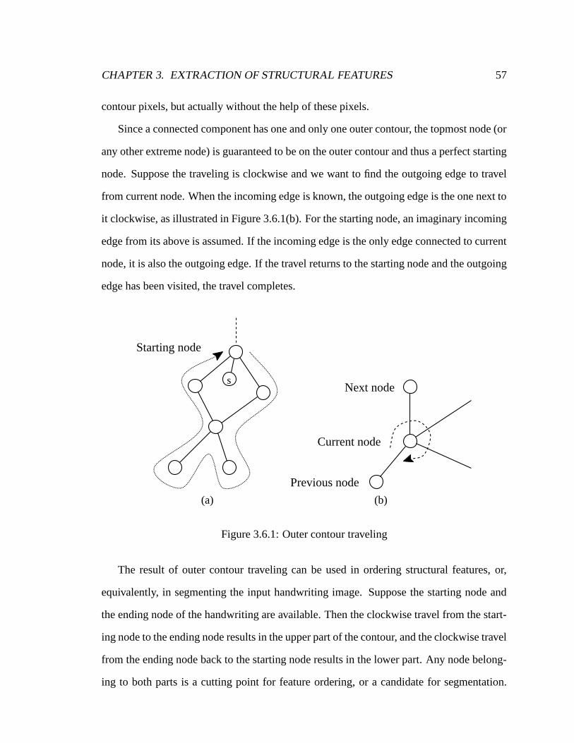
Figure 1.4.1: A graph representation of handwriting for structural feature extraction. (a)Original image. (b) Skeletal graph.

1.5 Proposed Approach

In this work, we will use the shape-defining structural features as the basic units in con-

structing models for word recognition. The major problems to be solved are:� How to extract features and order them in a sequence?� What modeling tool should be used to model sequences of structural features?� How to build character models and then word models on top of character models?� How to match a feature sequence efficiently against a word model?� How to evaluate a word recognizer? Especially performance as a function on the

lexicon?

These problems will be briefly addressed in the following sections. Further details can be

found in corresponding chapters.


1.5.1 Feature extraction

Pattern recognition based on graphs has been broadly studied and successfully applied to

fingerprint verification [36, 37], 2-D object recognition [38], face recognition [39]. In

handwriting recognition, graphs are intended to capture the high-level structures that are

embedded in a group of strokes. Figure 1.4.1 gives an example of representing handwriting

in graph form. The original image (Figure 1.4.1(a)) consists of pixels, from which the

identification of structures like loop, turns, junctions and ends is only easy to human eyes

but difficult to computers. In order to derive an effective algorithm for structural feature

extraction, the pixel image is converted into a skeletal graph (Figure 1.4.1(b)) where the

abstraction yields structures immediately.

A direct approach to building the skeletal graph of a pixel image is skeleton extraction,

which, however, is very time-consuming because of its multiple iterations on striping con-

tour pixels. Therefore, another approach using block adjacency graphs constructed from

horizontal runs [40] is adopted to meet this challenge more efficiently. Details will be given

in Chapter 3.

1.5.2 Modeling tool

According to the oscillation model of handwriting, when a structure is located at some

upper extremum, the next structure (in terms of writing order) is very likely to be located

at some lower extremum, and vice versa. That is, neighboring features are highly related

in position and orientation. Moreover, features extracted from a same character are usually

consistent except for some variations. For example, the character ‘d’ most likely consists

of a circle and an ascender unless the loop is broken or solid due to sloppy handwriting.

Therefore, feature sequences exhibiting strong dependence between neighboring features

are what to be modeled.

The proposed structural features may not be as good as statistical features derived from


pixels in recognizing characters, because they ignore some details of the handwriting, such

as how two structures are connected and by what kind of strokes. A similar problem is

also reported in [23], where the character recognition rate using grapheme features is only

about 30%, far less than the 95+% rate reported in [41, 42] where pixel-based features are

used. However, when structural features form a sequence, the length of the sequence and

the dependency between neighboring features can eliminate most of the word candidates

that are not the truth.

One straightforward approach to modeling sequences is to use prototypes/examples.

Each class consists of some prototypes of that class and the input is matched against all pro-

totypes one by one. The top few prototypes that have smallest distance to the input will be

used for classification purposes, such as in k-nearest neighbor approaches [43]. To compute

the distance between two sequences, edit distance [44] and its variants, such as constrained

edit distance [45] and normalized edit distance [46], have been widely adopted. Algorithms

for learning edit distance by stochastic transducers [47] are also available. However, one

limit of this approach is that the data’s inner structure is actually captured by enumeration

rather than generalization, which may result in unnecessarily large models, and another

limit is that it is not suitable for sequences of continuous values.

Currently, hidden Markov models (HMMs) prove to be very effective in handwriting

recognition [23, 25, 26]. HMMs are stochastic finite-state automata (SFSAs) exhibiting the

(1st order) Markovian property that a transition from one state to another state does not de-

pend on any previous states. This property is appropriate for modeling strong dependence

between neighboring observations/features. Since HMMs are usually also indeterministic

automata, there can be more than one state-transitioning sequence corresponding to an ob-

servation sequence. In this sense, the best state sequence to interpret the input is hidden

from us.

To be more general, this work starts with discussions on SFSAs, giving its training


and decoding algorithms. Then, HMMs are viewed as special SFSAs obtained by tying

parameters on transitions. Further details will be given in Chapter 2.

1.5.3 Modeling characters and words

The purpose of the training phase is to build word models that are to be matched against

input feature sequences in the recognition phase. Training can be done directly on word

images if the lexicon is fixed and small, like in reading the courtesy amount of a bankcheck.

For this kind of applications, it is feasible to gather sufficient amount of training images

for all words in the lexicon. However, a generic word recognizer should deal with lexicons

of various sizes ranging from tens of entries as in reading checks to tens of thousands of

entries as in reading US city names. It is possible for the recognizer to encounter words

that are not included in the training examples. Therefore, training character models and

concatenating them to obtain word models will be a more practical way to construct a

generic word recognizer.

Character models can be manually built as described in [24] if their number is small

and the feature extraction is quite easy to human eyes. Anyway, the task is tedious and

error-prone, so an approach to automating the character modeling procedure is necessary.

SFSAs and HMMs are chosen as the modeling tools because there exist efficient algorithms

for their training and decoding, so only little amount of human effort will be involved, such

as in designing the topology of underlying automata.

Since word models are built based on character models, there is an issue arising im-

mediately. Character images are segmented out from word images. As a result, ligatures

are generally broken into two parts that belong to two different neighboring characters. If

word models are built simply by concatenating character models trained on character im-

ages, broken ligatures will be prevailing in the resulting word model, which may be quite

contrary as in the real life cursive handwritings. This gives difficulties to recognizers that


are trying to utilize information about extrema, because broken ligatures in character ex-

amples introduce extrema that are not necessarily existing in the input word image. There

is still another problem also brought up by segmentation. Is the ordering of features when a

character is alone consistent with the ordering when the same character is in a word? If not,

the word templates built on character examples can never be used effectively. In order to

overcome the inconsistency between character images and word images, it is better to train

character models on word images, which is called embedded training, than on character

images directly.

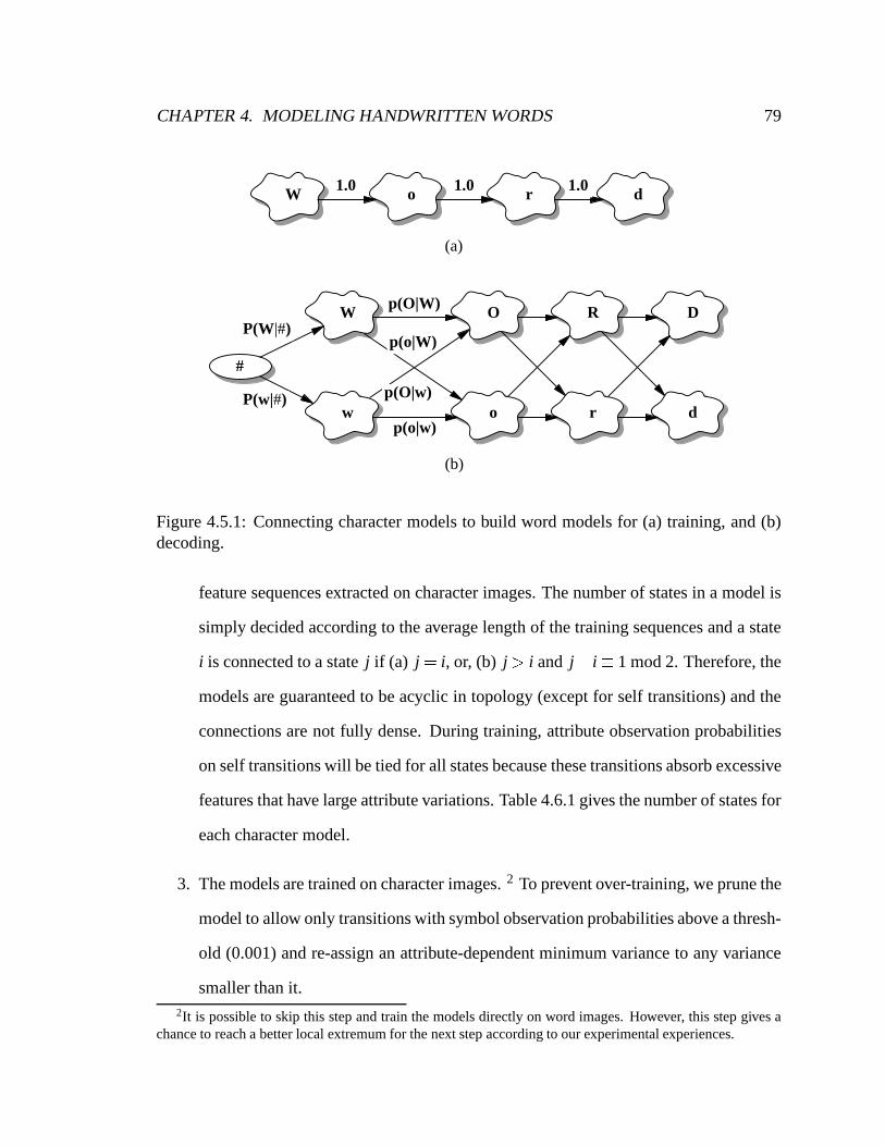
Chapter 4 will elaborate on the modeling of words on top of characters.

1.5.4 Fast decoding

After stochastic character models have been trained on character images and word images,

they are ready to be used in recognition. Besides accuracy, one major issue associated with

stochastic models is the decoding speed. It is commonly accepted in HMM-based speech

recognition that it is worthy of sacrificing some accuracy for speed. However, we are more

interested in techniques that allow fast decoding without losing accuracy.

In the study of a word recognizer based on over-segmentation and dynamic program-

ming on segment combinations [22], it is noticed that a character needs not to be matched

against the same handwriting segment more than once, so a substantial amount of com-

putation is saved when the same character appears multiple times in different words. The

same idea can be applied to our stochastic approach. To generalize this idea more, a string

of characters needs only be matched against the same handwriting segment once, which

validates not only the traditional prefix sharing technique for improving speed but also our

new suffix sharing technique.

Since a character can only consist of a limit number of structural features, duration

constraint, which specifies the maximum number and the minimum number of features a


character can have, will further reduce the computing time. However, this technique does

not guarantee exact decoding. Sometimes, a character may have more or fewer number of

features than expected. In these cases, the decoding result may be different from the result

when this technique is not used.

A parallel version of the stochastic word recognizer has been implemented by splitting

a large lexicon into several small lexicons of equal size. One processor is assigned to work

on one small lexicon and the results of all processors are combined to produce the overall

output.

Chapter 5 will describe the above techniques in more details and also give more speed-

improving techniques such as choice pruning and probability-to-distance conversion. In

some other thoughts, because the recognition process can be done in polynomial time,

more computing power in courtesy of Moore’s law 1 can be expected to conquer the speed

barrier and the accuracy issue will always be considered at the first place.

1.5.5 Performance evaluation

It is already known that the performance of a word recognizer depends on the lexicon.

Generally, large lexicons are more difficult than small lexicons; lexicons containing sim-

ilar words are more difficult than those containing totally different words. However, the

literature lacks a quantitative model to capture the dependence of a word recognizer’s per-

formance on lexicons. A common approach is to plot data gathered from extensive experi-

ments and observe from the plot the tendency of performance change when parameters are

altered [48, 49].

Since we build word recognition on top of character recognition, performance on word

recognition must be associated with performance on character recognition. And this asso-

ciation is through the lexicon. A extreme case is when the lexicon contains only entries of1Moore’s law: Computing power would rise exponentially (be doubled) over relatively brief periods of

time (18 months), by Gordon Moore, 1965


individual characters, word recognition degenerates to character recognition.

Two quantitative parameters are derived from the lexicon. One is the lexicon size and

the other is word similarity measured by the average edit distance between lexicon entries.

A performance model is inferred to associate word recognition accuracy with these two

parameters of lexicon. In this performance model, three model parameters are used to

characterize a word recognizer, one for the recognizer’s ability to distinguish characters

and two for the recognizer’s sensitivity to lexicon size.

Our performance evaluation methodology follows the analytical word reading theory

rather than the holistic one. So it will be applicable to analytical word recognizers but not

holistic ones. Chapter 6 gives details on the derivation of the model and the support of the

model from experiments.

1.6 Dissertation Outline

In Chapter 2, the theoretical basis of the whole dissertation, i.e. stochastic modeling, is

discussed. Starting with stochastic finite-state automata (SFSAs) which are less referred

to in the literature, we view hidden Markov models as special cases of SFSAs by tying

parameters on transitions. Chapter 3 describes an approach to structural feature extraction

based on skeletal graphs. Chapter 4 generalizes models discussed in Chapter 2 to model

structural features with continuous attributes. Chapter 5 investigates several fast-decoding

techniques, which in combination result in tens of times speed improvement for decoding

on large lexicons. Chapter 6 proposes a performance evaluation model to reveal the relation

between character recognition and word recognition in terms of performance. The model

parameters, which can be conveniently obtained by multiple regression, interpret a word

recognizer’s ability to distinguish characters and its sensitivity to lexicon size. Finally,

Chapter 7 summarizes this work and suggests future research directions.

Chapter 2

Stochastic Modeling

2.1 Introduction

In real world, we frequently encounter stochastic processes that produce observable out-

puts. The waveform of a speech, the movement of a pen in handwriting, and a gesture

signaling “come over here”, all come with a sequence of observations. One same meaning

can be always conveyed by multiple sequences for which sometimes we call accents, styles,

or even errors. It becomes difficult to recognize the true meaning of a stochastic process

when the variation in the resulting sequences is large. To tackle this problem systematically,

stochastic modeling based on probability theory is introduced.

In most literature, hidden Markov models (HMMs) represent the start-of-the-art of

stochastic modeling. HMMs are first successfully applied to speech recognition [50, 51,

52, 53, 54] and a good tutorial can be found in [55]. Nowadays, they attract more and more

interest of researchers in many other fields, including handwriting recognition [56, 23],

motion tracking (gesture recognition [57, 58], lipreading [59], etc.), information extraction

[60, 61], protein modeling [62, 63], robotic navigation [64, 65], and fingerprint classifica-

tion [66, 67].

14

CHAPTER 2. STOCHASTIC MODELING 15

With the physical layout as a network of connected states, HMMs are capable of de-

scribing the inner structure of complex data from a probabilistic view. HMMs satisfy the

(first-order) Markovian property that a transition from a state depends only on this state re-

gardless the state-transitioning history, i.e. how this state is reached. Generally, HMMs

are non-deterministic. One observation sequence can be interpreted by multiple state-

transitioning sequences. In this sense, the states of transition are hidden from the outside

observer.

HMMs can be viewed as special cases of stochastic finite-state automata (SFSAs) which

are generalizations of finite-state automata (FSAs). HMMs can be equivalently converted

into SFSAs but not generally the reverse. Therefore, after the problem of stochastic model-

ing is defined, we first discuss SFSAs, including the training and decoding algorithms, and

then view HMMs as the results of tying parameters of SFSAs.

2.2 Problem Definition

Stochastic modeling always has two phases: training and decoding. The training phase

derives stochastic models from training examples and the decoding phase matches an input

to candidate models, choosing the best one as the output. A training example and a de-

coding instance are in the same form, consisting of a sequence of observations. The only

difference is that a training example is accompanied with its truth but a decoding instance

is not.

2.2.1 Observations

Observations are the basic elements modeled by stochastic models. In speech recogni-

tion, they are usually some form of spectral feature vectors extracted from speech wave-

form [54]. However, in handwriting recognition, there are more choices of observations


due to the fact that handwriting can be either on-line or off-line and it is not exactly one-

dimensional.

In on-line handwriting recognition, temporal information about pen trace and pen pres-

sure is available, making good observations for modeling. Unfortunately, such information

is dropped when handwriting is provided off-line. Many different feature extraction meth-

ods have been proposed by researchers to deal with this difficult situation and they can be

divided into two categories: statistical and structural. The first category is to treat handwrit-

ing script as one-dimensional signal from left to right and extract statistical features from a

sliding window [56, 26]. Statistical features are relatively straightforward to extract, but the

simplifying assumption that handwriting is one-dimensional makes them weak in capturing

two-dimensional structures like circles, loops and crosses. The second category emphasizes

on the extraction of structural features and the ordering of them sequentially [24, 23, 40].

It views handwriting as two-dimensional structures linked one-dimensionally. Since this

view resembles more closely to human’s recognition of handwriting, it generally leads to

more promising results. Table 2.2.1 gives a brief comparison of off-line word recognition

results in the two categories reported in literature. It is hard to say what type of recognizers

is better because the results compared are not obtained on the same testing set. What can

be seen is that researchers are paying increasing attention to the use of structural features

in handwriting recognition.

2.2.2 Stochastic training

Define an observation sequence to be O �� o1 o2 �� oT � where ot are from an alphabet

of observations. In speech recognition, the index to observations is called “time” because

observations are obtained by sampling the waveform in time frames. In handwriting recog-

nition, although there is no such temporal property of observations, it will be convenient to


Work Year Approach Testing data Result on lexicons of size10 100 1000

[56] 1995 HMM US postal names 93% 81% 63%[26] 1996 HMM&DP US postal names 89%[68] 1996 DP US postal names 97% 91% 81%[22] 1997 DP US postal names 97% 88% 74%

(a) Using statistical features

Work Year Approach Testing data Result on lexicons of size10 100 1000

[24] 1998 DP US postal names 99% 95% 86%[23] 1999 HMM French city names 99% 96% 88%

(b) Using structural features

Table 2.2.1: Comparison of results reported in the literature, using statistical features andstructural features.

just follow the existing convention in speech recognition and still call the index to observa-

tion as “time”.

Now let λ be a stochastic model representing the knowledge on a class to be distin-

guished. The problem of stochastic training for λ can be described as follows.

Input: A set of observation sequence O1 O2 �� ON.

Output: A model λ � argmaxλP � λ �O1 O2 �� ON � .The output model λ consists of two parts: (a) model topology including the number of

states and inter-state connections, and (b) model parameters defining the probabilities of

transitioning between states and/or that of emitting observations.

In most work reported in literature, the common approach to stochastic training is to

first define the model topology manually or by some heuristics, and then train model pa-

rameters on examples to refine the model. During the training, pruning can be performed

to remove low-probability transitions, thus re-defining the model topology.

Theoretically, model topology can be trained as well as model parameters. For instance,


HMMs are studied in the field of information extraction where the key information is asso-

ciated with some prefix and also some suffix. Freitag and McCallum [61] introduce a set

of topological operations, such as lengthening a prefix/suffix and splitting a prefix/suffix,

to refine the model topology. In the field of on-line handwriting recognition, Lee et al. [69]

propose a method of designing HMM topology by clustering examples and assigning dif-

ferent number of states to each cluster. Experiments on on-line Hangul1 recognition show

about 19% of error reduction compared to the intuitive model topology design. However,

in their method, the model topology for a cluster is still sequentially left-to-right.

Although the above-described techniques prove to be successful in their domain, they

cannot be readily applied to other fields because they make structural assumptions about

the model topology. So we are looking for some other methods that do not make such

assumptions.

According to the Bayes rule, one has

P � λ �O1 O2 �� ON �� P � O1 O2 �� ON � λ � P � λ �P � O1 O2 �� ON � � (2.2.1)

Since P � O1 O2 �� ON � is fixed in the selection of the best model, it can be ignored in

argmax.

argmaxλP � λ �O1 O2 �� ON �� argmaxλP � O1 �O2 ��ON � λ � P � λ �

P � O1 �O2 ��ON �� argmaxλP � O1 O2 �� ON �λ � P � λ � � (2.2.2)

So there are two factors to consider, P � O1 O2 �� ON �λ � , the likelihood of the observa-

tions being produced by the model, and P � λ � , the prior probability of having the model. The

likelihood can be efficiently calculated by the famous Balm-Welch algorithm [70] which is

also known as the Forward-Backward algorithm. However, how to get the prior is not obvi-

ous and, actually, it implies the preference of one model over another when no observation1A Korean phonetic writing system


is made.

2.2.3 Stochastic decoding

A stochastic decoding problem can be defined as follows.

Input: a) A set of candidate models Λ �� λ1 λ2 �� and

b) An observation sequence O �� o1 o2 �� oT � .Output: The best model λ � argmaxλ � ΛP � λ �O � .

Here the candidate models are obtained in the stochastic training phase and it needs to

be decided which one of them best interprets the given observations. The Bayes rule says

P � λ �O �� P � O �λ � P � λ �P � O � (2.2.3)

and leads to

argmaxλ � ΛP � λ �O �� argmaxλ � ΛP � O � λ � P � λ �

P � O �� argmaxλ � ΛP � O �λ � P � λ � (2.2.4)

where P � O � is finally ignored in the argmax for it is constant in selecting the best model.

So, similarly to the situation in stochastic training, there are also two factors to consider,

P � O � λ � , the likelihood of observation sequence O being produced by model λ, and P � λ � ,the prior probability of having λ when no observations are given.

Unlike the prior described in stochastic training, which is very important in searching

a best model topology in an unlimited space, the one here is quite simple because the best

model must be one of the models in Λ that is already given. The prior can be obtained by

simple statistics such as normalized character frequencies in handwritten character recogni-

tion or by language models such as N-gram syntax models in speech recognition. When the

prior is not available, it can be reasonably assumed to be the same for all models. There-

fore, we are more interested in computing the likelihood part P � O � λ � than the prior part


0 1 2

a

b

a b3

b

a

0 1 2

b

a b3

b

a a

b

(a) non-deterministic (b) deterministic

Figure 2.3.1: Examples of deterministic and non-deterministic FSAs, both modeling regu-lar language � a � b � � abb.

P � λ � .2.3 Finite-State Automata

Finite-state automata (FSAs) are the visualized forms of regular expressions, the type 3

languages lying in the bottom of the Chomsky formal language hierarchy [71]. Though

not as powerful as other language types, regular expressions are easy to harness for their

simplicity and have been integrated into many programming languages, like Perl, Java and

Python, as the basic string pattern matching tool.

FSAs can be either deterministic or non-deterministic and the latter can be equivalently

converted to the former. If an automaton seeing an input symbol at some state is always

certain about the next state to transition to, then it is deterministic; otherwise, it is non-

deterministic. Figure 2.3.1 gives examples of these two types of automata, both modeling

the same regular language � a � b � � abb. It can be readily seen that the non-deterministic

version is more concise than its deterministic counterpart. Generally speaking, the size of a

non-deterministic FSA can be no larger than a deterministic one when they model the same

language. Therefore, it is not necessary to remove the uncertainty in non-deterministic

FSAs.

Martino et al. [72] studied an interesting topic about choosing between HMMs and


FSAs in speech recognition. In their study, a deterministic FSA in prefix-tree format is

built to exhaustively represent the training space and dynamic programming is used to

decode an input. Experiments on the Texas Instruments Tidigits database show similar

performance of the FSA approach compared to an HMM approach. Despite of the result

presented, this study ignores the fact that HMMs are stochastic generalizations of FSAs.

Representing the training space exhaustively is only desirable when the space is relatively

small. The claim that deterministic FSAs are as accurate as HMMs actually supports the

effective use of HMMs as generalizations of FSAs.

In order to give FSAs more modeling power and to keep them from exploding in size

when the training space is large, probability distributions of observations on the transitions

are introduced, resulting in stochastic FSAs.

2.4 Discrete Stochastic Finite-State Automata

Generally speaking, the input observations to a stochastic finite-state automaton (SFSA)

can be either from a set of discrete symbols, which is usually also finite, or a set of con-

tinuous values, which is definitely infinite. The model is called discrete for the former

case and continuous for the later case. The distribution of symbols can be simply mod-

eled by discrete probabilities. However, probability density functions (typically Gaussian

distributions) are necessary to model continuous observations.

For simplicity and clarity, we start discussions on discrete SFSAs, introducing the defi-

nition, the training algorithm, and the decoding algorithm. The next chapter will deal with

continuous SFSAs with less elaboration since all the major concepts still hold.


2.4.1 Definition

To model sequences of discrete observations, we define a discrete SFSA λ �� S L A as

follows.� S �!� s1 s2 �� sN � is a finite set of states, assuming single starting state s1 and single

accepting state sN .� L is a finite set of discrete symbols, making an alphabet of observations. A special

null symbol ε is not included in L. It appears only in the model definition but not in

the input observations. No observation is required to match the null symbol.� A �"� ai j � o � � is a set of observation probabilities, where ai j � o � o # L $%� ε � , is the

probability of transitioning from state i to state j and observing o. When a model

observes the null symbol, it does not observe anything in the input. A constraint is

placed on observation probabilities: the sum of a state’s outgoing probabilities must

equal to 1, i.e. ∑ j ∑o ai j � o �� 1 for all state i.

Although this definition includes the assumption of single starting state and single ac-

cepting state, it does not mean any reduced modeling power. A traditional definition may

give an initial distribution π of starting states and a set of accepting states. In this case,

the network topology can be slightly modified to conform to the assumption. First a new

single starting state is connected to all old starting states, with the same distribution π of

emitting null symbols on all connections. And then all old accepting states are connected

to a new single accepting state, with probability 1 emitting null symbols 2. This assump-

tion is important if one needs to build large models by concatenating small models, such as

concatenating character models to obtain word models in word recognition. Single-entry

and single-exit models make the concatenation much easier.2This setting of probability may violate the constraint that the sum of a state’s out-going probabilities

must be 1. Anyway, they can be normalized to meet the constraint.


Si Sj

0.1 0.2

0.30.4

ε 0.2 ε 0.1

0.5 0.2Sk

Figure 2.4.1: Transitions in the context of handwriting recognition, where structural fea-tures like cross, loop, cusp and circle are used in modeling.

Figure 2.4.1 gives an example of transitions in the context of handwriting recognition.

Symbols like cross, upward loop, upward cusp, circle, downward loop, downward cusp

and null are observed on transitions between states. Probabilities are associated with the

observations and satisfy the constraint that a state’s outgoing probabilities must sum to 1.

We can draw some analogy between the model structure and the edit distance opera-

tions including insertion, deletion and substitution. Firstly, self transitions (from a state to

itself) correspond to insertions that absorb extra observations in the input. Secondly, tran-

sitions from one state to another state observing the null symbol correspond to deletions

that compensate for missing observations in the input. Thirdly, all other transitions corre-

spond to substitutions that allow alternatives in the input. Fourthly, the negative logarithm

of an observation probability can be interpreted as the edit cost. Of course, the major dif-

ference is that all operations and costs have been made dependent on the context where the

transitions are taken in the model.

It should be pointed out that null self-transitions are not allowed in the model. Such

transitions change neither the state nor the time (index to observations). If they are taken,

the status of the automaton remains the same. So it is meaningless to consider null self-

transitions.

The input to a model is always an observation sequence O �� o1 o2 �� oT � where ot #L, with the truth given in training and without it in decoding. Because an SFSA is not

required to be deterministic, multiple state-transitioning sequences, i.e. paths from the


starting state to the accepting state, exist to interpret a given input. In this sense, we can

also call SFSAs as hidden state models, as we call HMMs.

Define a new predicate Q � t i � which is true when the model is in state i at time t. A state

sequence is denoted as Q � t0 q0 � Q � t1 q1 � �� Q � tW qW � , where 0 & tk & T and qk # S. The

state sequence must start from state 1 at time 0 and end to state N at time T , which means

t0 � 0, q0 � 1, tW � T and qW � SN . One more constraint is that tk ' tk ( 1 must be either 0

or 1. When tk ' tk ( 1 � 0, the null symbol is observed on the transition from state qk ( 1 to

state qk; otherwise, a non-null symbol is observed. So, by definition, the state sequence is

always longer than the observation sequence.

Three basic problems are to be solved in this stochastic framework.

1. How to calculate the probability of having an input given the model? That is, to

calculate the likelihood P � O � λ � .2. How to adapt model parameters to training examples? That is, to find the best model

λ � argmaxλP � λ �O � .3. What is the best (hidden) state sequence to interpret the input?

For the first two problems, the solutions are in the Forward-Backward training algorithm

[70]. For the last problem, the Viterbi decoding algorithm [73, 74] provides the solution.

Details will be given in later sections.

2.4.2 Training

The training is done by the Forward-Backward or Baum-Welch algorithm, which is a sub-

case of the Expectation-Maximization (EM) algorithm [75] and guarantees to converge

to some local extremum. This algorithm has two steps. The first step is the calculation

of forward and backward probabilities (defined later), giving solution to problem 1; and


the second step is the re-estimation of model parameters using the forward and backward

probabilities obtained in the first step, giving solution to problem 2.

Forward and backward probabilities

In order to train an SFSA efficiently, two important concepts, namely the forward proba-

bility and the backward probability, are introduced by the Forward-Backward algorithm.

(That is also how the name “Forward-Backward” comes.)

The forward probability α j � t �)� P � o1 o2 �� ot Q � t j �*�λ � is defined as the probability of

being in state j after the first t observations given the model. By this definition, one must

consider all possible paths reaching state j at time t, which can be numerous in the model

network. Fortunately, this can be done recursively as in the following equation,

α j � t �� +,- ,. 1 j � 1 t � 0

∑i � αi � t � ai j � ε �0/ αi � t ' 1 � ai j � ot �� otherwise (2.4.1)

which also implies an efficient dynamic programming algorithm. The first term in the sum

accounts for observing a null symbol, which does not consume any input observation, and

the second term accounts for observing some non-null symbol in the input. Figure 2.4.2(a)

illustrates the idea of this recursive computation.

The backward probability βi � t �1� P � ot 2 1 ot 2 2 �� oT Q � t i �*�λ � is defined as the prob-

ability of being in state i before the last T ' t observations given the model. It can be

calculated recursively as follows.

βi � t �3� +,- ,. 1 i � N t � T

∑ j � ai j � ε � β j � t �0/ ai j � ot 2 1 � β j � t / 1 �� s otherwise(2.4.2)

Similarly, the two terms in the sum account for observing the null symbol and some non-

null symbol in the input, respectively. An illustration of this recursive computation is given


in Figure 2.4.2(b).

Finally, αN � T �4� β1 � 0 �5� P � O �λ � is the overall probability of having the input given

the model, which solves problem 1.

Re-estimation

Before an SFSA is trained, all its transitions are initialized with the same observation prob-

ability. Such a flat model is useless for any recognition purpose. So, the central topic is to

re-estimate these observation probabilities based on the training examples. To simplify, we

first consider the re-estimation algorithm when there is only one training example and then

generalize the result to multiple examples.

Suppose the model to be trained is λ and the single training example is O �6� o1 o2 �� oT � .We feed the example to the model and calculate the likelihood P � O �λ � using the Forward-

Backward algorithm. Obviously, different transitions contribute differently to P � O �λ � dur-

ing the calculation. Some transitions might get excited by several paths and some others

might just remain silent because their possible observations do not appear in the input ex-

ample. Therefore, if observation probabilities are adjusted according to their contributions

to P � O �λ � , then the model is adapted to the example.

In this learning process, the probability of observing a symbol o # L $7� ε � while tran-

sitioning from state i to state j can be re-estimated as

Number of times observing o while transitioning from state i to state jTotal number of times transitioning from state i to any state and observing any symbol

according to the constraint that a state’s outgoing probabilities must sum to 1.

Since there are two types of observations, null and non-null, and they incur different

changes in time, we define two types of probabilities for them respectively.

ωi j � t �3� P � Q � t i � Q � t j �*�O λ � (2.4.3)


1

i

j N

αi(t-1)

αj(t) αN(T)α1(0)=1

αi(t)

ε ot

ε ot

ε ot

(a) Forward probability

1 i

j

N

βj(t+1)

βj(t)

ε

ot+1 βN(T)=1β1(0) βi(t)ε

ot+1

ε ot+1

(b) Backward probability

Figure 2.4.2: Calculation of forward and backward probabilities for stochastic finite-stateautomata. Time does not change if the null (ε) symbol is observed and time increases by 1if a non-null symbol is observed.


is the probability of observing ε while transitioning from state i to state j at time t, and

τi j � t �� P � Q � t ' 1 i � Q � t j �*�O λ � (2.4.4)

is the probability of observing a non-null symbol while transitioning from state i at time

t ' 1 to state j at time t. Once these two probabilities are available, the observation proba-

bilities can be re-estimated as

ai j � o �� +,- ,. ∑t ωi j � t �∑ j ∑t � ωi j � t �82 τi j � t �8� o � ε

∑t 9 ot : o τi j � t �∑ j ∑t � ωi j � t �82 τi j � t �8� o ;� ε

� (2.4.5)

The two equations have the same denominator, the expected number of transitions from

state i, including both null and non-null observations. ∑t ωi j is the number of times observ-

ing ε while transitioning from state i to state j. ∑t � ot < o τi j is the number of times observing

o while transitioning from state i to state j. The condition ot � o is necessary because there

are different non-null observations.

Although the re-estimation of observation probabilities has already been derived, the

two probabilities ωi j � t � and τi j � t � are still to be computed. According to the laws of joint

probability and conditional probability, we have

P � x �O λ �� P � x O � λ �P � O �λ � � (2.4.6)

Consequently,

ωi j � t �� P � Q � t i � Q � t j �=�O λ �>� P � Q � t i � Q � t j � O � λ �P � O � λ � (2.4.7)

and

τi j � t �� P � Q � t ' 1 i � Q � t j �*�O λ �)� P � Q � t ' 1 i � Q � t j � O �λ �P � O �λ � � (2.4.8)


1 i

αi(t)α1(0)=1

j N

βN(T)=1

βj(t)

εot

βj(t)

αi(t-1)

Figure 2.4.3: The probability of taking a transition from state i to state j observing eithernull or ot , given the model λ.

Equation 2.4.7 and 2.4.8 are easy to calculate based on forward and backward proba-

bilities. First, the denominator P � O � λ � is available as αN � T � or β1 � 0 � . Secondly, the two

numerators can be also obtained by

P � Q � t i � Q � t j � O � λ �� P � o1 o2 �� ot Q � t i �*�λ � ai j � ε � P � Q � t j � ot 2 1 ot 2 2 �� oT � λ �� αi � t � ai j � ε � β j � t � (2.4.9)

and

P � Q � t ' 1 i � Q � t j � O �λ �� P � o1 o2 �� ot ( 1 Q � t ' 1 i �=� λ � ai j � ot � P � Q � t j � ot 2 1 ot 2 2 �� oT �λ �� αi � t ' 1 � ai j � ot � β j � t � (2.4.10)

Figure 2.4.3 illustrates the calculation.

So far, the model is trained on one single example and biased only to it. For more reli-

able re-estimation, multiple examples must be used. In this case, the application of Equa-

tion 2.4.5 is delayed until all examples have been fed to the model, and the re-estimation is


performed over the accumulations of ωi j � t � and τi j � t � , i.e.

ai j � o �� +,- ,. ∑O ∑t ωi j � t �∑O ∑ j ∑t � ωi j � t �82 τi j � t �8� o � ε

∑O ∑t 9 ot : o τi j � t �∑O ∑ j ∑t � ωi j � t �82 τi j � t �8� o ;� ε

� (2.4.11)

It should be pointed out that the t variable is dependent on O, taking range from 1 to �O � .Such dependence is not shown in the equation for clean typesetting.

Since the re-estimation is based on the EM algorithm which guarantees to converge

to some local maximum, it can be done iteratively on the training data until ∑O P � O �λ �reaches a local maximum.

2.4.3 Decoding

The calculation of forward and backward probabilities already produces the likelihood

of an input, i.e. P � O � λ � , so a model that best interprets the input can be chosen as λ �argmaxλ � ΛP � O �λ � when the set of candidate models Λ is given. When the prior P � λ � is

available, the best model will be λ � argmaxλ � ΛP � O �λ � P � λ � .Forward/backward probabilities are capable of producing the likelihood of an input

given the model. However, a very important question is not answered yet. (Problem 3)

What is the best state sequence that produces the input observation sequence? If this is

answered, it also gives a best segmentation of the input when the model taking the input is

a concatenation of sub-models. Model concatenation is very common in stochastic model-

ing. In natural language processing, sentence models are built on top of word models, and

word models are on phoneme models for speech recognition or on character models for


λ2

time0 T

o1 o2 oi... oj+1 oj+2 oT...oi+1 oi+2 oj...

λ1 λ3

Figure 2.4.4: Deciding the best state sequence for an input, hence producing the best seg-mentation of the input.

handwriting recognition. Take Figure 2.4.4 for example. Three sub-models are concate-

nated to match the input. The forward/backward probabilities give the likelihood by

P � O �λ �3� ∑i � j s � t � i ? j

P � o1 o2 �� oi � λ1 � P � oi 2 1 oi 2 2 �� o j �λ2 � P � o j 2 1 o j 2 2 �� oT � λ3 � (2.4.12)

which is the sum of likelihoods of all possible state sequences including the best one.

However, it is better to know what are the most probable segmentation points i � and j �such that

i � j � � argmaxi � j s � t � i ? jP � o1 o2 �� oi � λ1 � P � oi 2 1 oi 2 2 �� o j � λ2 � P � o j 2 1 o j 2 2 �� oT �λ3 � �(2.4.13)

So we will know o1 o2 �� oi @ belong to the first sub-model, oi @A2 1 oi @B2 2 �� o j @ belong to the

second and o j @C2 1 o j @B2 2 �� oT belong to the third. Such information is extremely useful to

evaluate if a word recognizer is able to recognize individual characters in the word correctly.

In order to find the best state sequence for an input, the decoding is actually done by the

Viterbi algorithm. Define γi � t � , the Viterbi probability, as the highest probability of being

in state i at time t produced by one state sequence, then it can be recursively calculated as


follows.

γ j � t �3� +,- ,. 1 j � 1 t � 0

max � maxi γi � t � ai j � ε � maxi γi � t ' 1 � ai j � ot �� otherwise(2.4.14)

The null symbol and non-null symbols are considered separately, as done in calculating

forward and backward probabilities. This equation is different from Equation 2.4.1 in that

probabilities resulting from incoming transitions are not accumulated. Instead, only the

highest probability is kept by the max operator. Finally, γN � T � is the Viterbi probability of

observing the entire input given the model.

The best state sequence can be retrieved by backtracking. The last state is obviously

Q � T N � , being in state N at time T . In backtracking, we need to consider null sym-

bol and non-null symbol separately. If γ j � t �D� maxi γi � t � ai j � ε � , then the previous state

is Q � t argmaxi γi � t � ai j � ε �� . If γ j � t �E� maxi γi � t ' 1 � ai j � ot � , then the previous state is

Q � t ' 1 argmaxi γi � t ' 1 � ai j � ot �� . This backtracking proceeds until Q � 0 1 � , being in state

1 at time 0, is reached.

2.4.4 Complexity analysis

As defined previously, N is the number of states in a model and T is the number of obser-

vations in the input. Suppose there are M transitions in the model. So the average incoming

degree of a state is M F N.

For simplicity, the time of taking one transition is considered as the unit time.

Forward-Backward algorithm

The algorithm consists of three major steps, each analyzed as follows.� According to Equation 2.4.1 and 2.4.2, there are 2NT values of α j � t � and βi � t � to


calculate. And the average cost of calculating a value is M F N, the average incoming

degree of a state, hence the cost of this step is 2MT .� In Equation 2.4.7 and 2.4.8, there are 2MT values of ωi j � t � and τi j � t � , and the calcu-

lation of a value costs O(1). So the cost of this step is also 2MT .� The re-estimation initiated by Equation 2.4.11 is performed only once for all training

examples, so its cost can be viewed as amortization and ignored when the number of

examples is large.

Therefore, the overall complexity of the Forward-Backward algorithm on a single input is

O(MT ).

Viterbi algorithm

According to Equation 2.4.14, there are NT many γ j � t � values to calculate and the average

cost of each γ j � t � calculation is 2M F N. Therefore, the overall complexity is O(MT ) for a

single input.

2.5 Hidden Markov Models

Unlike SFSAs which emit observations on transitions, HMMs emit observations on states.

Figure 2.5.1 shows an example of HMM in the context of handwriting recognition.

Similar to SFSAs, HMMs are also stochastic generalizations of FSAs. Not surprisingly,

HMMs can be viewed as special cases of SFSAs by tying observation probabilities that

are on the transitions to the same state. According to this view, their training/decoding

algorithms can be derived easily from those of SFSAs. The following sections will give the

details.


Si Sj0.9

0.1 0.2

0.3

0.4

ε 0.2

0.8

ε 0.1

0.6

0.3

Sk

0.1

ε 0.4

0.6

Figure 2.5.1: An example of HMM in the context of handwriting recognition.

2.5.1 Viewing HMMs as special SFSAs

Figure 2.5.2 gives an example of converting an SFSA to an HMM and vice versa. Given

an SFSA (2.5.2(a)), its observation probabilities on a transition can be decomposed into

two parts (Figure 2.5.2(b)). The first part is the sum of observation probabilities on the

transition, which corresponds to the concept of transition probability in HMMs, and the

second part is the weight of an observation among all observations on the transition, which

corresponds to the concept of emission probabilities in HMMs. Then, by averaging/tying

emission probabilities on the transitions to the same state (state 3), we obtain an HMM in

Figure 2.5.2(c) using the calculation in Figure 2.5.2(e). Figure 2.5.2(d) shows an SFSA

which is equivalent to the HMM but different from the original SFSA.

The conversion from SFSA to HMM loses information but the conversion from HMM

to SFSA does not. Figure 2.5.2(f) shows that parameter tying results in flattened distribu-

tion of strings.


1

3

2

a, 0.05 b, 0.30 c, 0.05

a, 0.05 b, 0.05 c, 0.20

0

a, 0.05 b, 0.05 c, 0.25

a, 0.50 b, 0.10 c, 0.05

1

3

2

0.40 x a, 0.13 b, 0.75 c, 0.13

0.30 x a, 0.17 b, 0.17 c, 0.67

0

0.35 x a, 0.14 b, 0.14 c, 0.72

0.65 x a, 0.77 b, 0.15 c, 0.08

(a) SFSA (b) Another view of SFSA

1

3

2

0.40

0.30

0

0.35

0.65

a, 0.14 b, 0.14 c, 0.72

a, 0.77 b, 0.15 c, 0.08

a, 0.15 b, 0.41 c, 0.44 1

3

2

a, 0.06 b, 0.16 c, 0.18

a, 0.05 b, 0.12 c, 0.13

0

a, 0.05 b, 0.05 c, 0.25

a, 0.50 b, 0.10 c, 0.05

(c) HMM from SFSA (d) SFSA from HMM

String � Prob. Normalized prob.?a 0.0500 0.15?b 0.1375 0.41?c 0.1475 0.44

sum 0.3350 1.00� ? stands for any one symbol

String SFSA prob. HMM prob.ab 0.0400 0.0697ac 0.1025 0.0748cb 0.0775 0.0472cc 0.0225 0.0506

sum 0.2425 0.2423

(e) Emission prob. (f) String prob.

Figure 2.5.2: Converting a stochastic finite-state automaton (SFSA) to a hidden Markovmodel (HMM) by parameter tying. (a) The original SFSA. (b) The view of observationprobabilities as transition probabilities times emission probabilities for SFSA . (c) HMMobtained by tying emission probabilities from state 1 to state 3 and those from state 2 tostate 3. (d) Equivalent SFSA converted from HMM. (e) The calculation of tied emissionprobabilities for state 3. (f) Probabilities of generating some strings by the original SFSAand the HMM.


2.5.2 Definition

In the definition of a discrete SFSA (Section 2.4.1), the transition from state i to state j

is associated with a probability distribution ai j � o � of observing o on this transition. A

constraint that the sum of a state’s outgoing probabilities must equal to 1, i.e. ∑ j ∑o ai j � o �)�1, is placed on all states i.

According to the view of HMMs as special SFSAs by tying observation probabilities,

the observation probability ai j � o � is now decomposed into two parts

ai j � o �� bi jc j � o � (2.5.1)

where bi j is the transition probability and c j � o � is the emission probability. Unlike in

an SFSA, the symbols are observed on (or emitted by) states instead of transitions in an

HMM. Two new constraints on the probabilities are introduced. Firstly, the sum of tran-

sition probabilities from a state must be 1, i.e. ∑ j bi j � 1. Secondly, the sum of emis-

sion probabilities of a state must be 1, i.e. ∑o c j � o �G� 1. These two constraints guarantee

∑ j ∑o ai j � o �H� ∑ j ∑o bi jc j � o �1� ∑ j I bi j ∑o c j � o �KJL� 1, which is the constraint on the obser-

vation probabilities for an SFSA.

Finally, the definition of a discrete HMM λ �M� S L B C is given as follows.� S �!� s1 s2 �� sN � is a finite set of states, assuming single starting state s1 and single

accepting state sN .� L is a finite set of discrete symbols. A special null symbol, represented by ε and not

included in L, appears only in the model definition but not in the input observations.� B �N� bi j � is a set of transition probabilities from state i to state j. The sum of

transition probabilities from a state must be 1, i.e. ∑ j bi j � 1.� C �� c j � o � � is a set of emission probabilities of observing/emitting o # L $O� ε � on


state j. The sum of emission probabilities on a state must be 1, i.e. ∑o c j � o �� 1.

2.5.3 Training

After the training procedure for SFSAs, the training of HMMs becomes straightforward.


By applying the equality ai j � o �� bi jc j � o � , forward and backward probabilities for HMMs

are directly obtained from Equation 2.4.1 and 2.4.2.

α j � t �� +,- ,. 1 j � 1 t � 0

∑i � αi � t � bi jc j � ε �L/ αi � t ' 1 � bi jc j � ot �� otherwise (2.5.2)

βi � t �3� +,- ,. 1 i � N t � T

∑ j � bi jc j � ε � β j � t �0/ bi jc j � ot 2 1 � β j � t / 1 �� s otherwise(2.5.3)

Re-estimation

Since the observation probabilities in an SFSA are decomposed into transition probabilities

and emission probabilities in an HMM. Equation 2.4.5 for the re-estimation of observation

probabilities must be decomposed accordingly.

By replacing ai j � o � with bi jc j � o � , we compute ωi j � t � and τi j � t � using the same equa-

tions as in training SFSAs (Section 2.4.2).

For transition probabilities, the re-estimation equation is

bi j � ∑t � ωi j � t �0/ τi j � t ��∑ j ∑t � ωi j � t �0/ τi j � t �� (2.5.4)

where the denominator is still the total number of transitions from state i but the numerator


is the number of transitions from state i to state j. This re-estimation is based on the

constraint ∑ j bi j � 1.

For emission probabilities, the re-estimation equation is

c j � o �� +,- ,. ∑i ∑t ωi j � t �∑i ∑t � ωi j � t �82 τi j � t �8� o � ε

∑i ∑t 9 ot : o τi j � t �∑i ∑t � ωi j � t �82 τi j � t �8� o ;� ε

� (2.5.5)

In both cases, the denominator is the number of transitions to state j. The numerator in the

first case is the number of times that the null symbol is emitted by state j. The numerator

in the second case is the number of time that a non-null symbol o is emitted by state j. The

use of ∑i enforces the tying of observation probabilities on all the transitions from some

state i to the same state j. This re-estimation is based on the constraint ∑o c j � o �� 1.

2.5.4 Decoding

Similarly, by replacing ai j � o � with bi jc j � o � , we obtain Viterbi decoding for HMMs from

Equation 2.4.14.

γ j � t �� +,- ,. 1 j � 1 t � 0

max � maxi γi � t � bi jc j � ε � maxi γi � t ' 1 � bi jc j � ot �� otherwise(2.5.6)

The best state sequence can be also obtained by the same backtracking procedure as for

SFSAs.


There is no complexity difference in terms of order of magnitude between training/decoding

SFSAs and training/decoding HMMs.

The same complexity analysis for SFSAs (Section 2.4.4) applies for HMMs. Therefore,


the complexity of the Forward-Backward algorithm on a single input is O(MT ) and that of

the Viterbi algorithm on a single input is also O(MT ), where M is the number of transitions

in the model and T is the number of observations in the input.

2.6 Conclusions

In this chapter, we have defined (discrete) stochastic finite-state automata (SFSAs). The

training algorithm for them is a variant of the famous Forward-Backward algorithm and the

decoding algorithm is the well-known Viterbi algorithm. In both algorithms, we rigorously

consider the use of null symbols which is rarely dealt with in literature. Both algorithms

have time complexity O(MT ) on a single input, where M is the number of transitions in the

model and T is the number of observations in the input.

We also view hidden Markov models (HMMs) as special cases of SFSAs by tying

observation probabilities. Training and decoding algorithms for HMMs are derived directly

from those for SFSAs, attaining the same time complexity.

Observations are emitted by transitions in an SFSA but they are emitted by states instead

in an HMM. Since the number of transitions in a model is generally more than the number

of states, an SFSA has the ability of modeling data in more details than does an HMM.

In Chapter 4, we will apply both SFSAs and HMMs in the context of off-line cursive

handwritten word recognition and compare their performance.

Chapter 3

Extraction of Structural Features

3.1 Introduction

In image pattern recognition, skeletal graphs are graphs representing the relation between

image components. When an image is properly decomposed, the resulting skeletal graph

is capable of capturing high-level structures in the image without engaging in the low-level

details. Skeletal graphs play a very important role in syntactic and structural pattern recog-

nition. Kupeev and Wolfson [76] have developed G-graphs, representing skeletal structure

of images, as in measuring the similarity between two 2-D objects. Kato and Yasuhara

[77] have proposed an approach to recovering drawing order of handwritten scripts based

on skeletal graphs. Dzuba et al. [24] have applied skeletal graphs in building a high-

performance word recognizer which utilizes the recognition power of structural features.

A direct approach to building skeletal graphs is based on thinning. After the image

skeleton is obtained, connectivity analysis is done on all skeletal pixels: 1-degree 1 pixels

forming end nodes, 2-degree pixels forming edges, and other pixels forming inner nodes.

However, this process may introduce spurious lines that do not exist in the original image,

typically happening at the intersection of two strokes. To solve this problem, Kato and1The degree of a pixels is defined as the number of neighboring pixels in the skeleton.

40

CHAPTER 3. EXTRACTION OF STRUCTURAL FEATURES 41

Yasuhara[77] apply a clustering algorithm to merge pixels near a spurious line into a single

inner node. Fan et al. [37] proposed another method of skeletonization by block decom-

position and contour vector matching. The input image is first decomposed into blocks

of vertical runs 2, then block contours are vectorized and vectors matched to get skeletal

vectors. Extra processing near intersections is required to find the appropriate point to join

vectors.

In this chapter, a new method of building skeletal graphs without skeleton extraction

is proposed for handwriting images. It aims at the extraction of structural features from

cursive handwriting scripts. These features are loops, turns, ends and junctions, most of

which are near vertical extrema due to the fact that handwriting is approximately an up-

down oscillation from left to right. Firstly, the input image is converted into horizontal

runs upon which a block adjacency graph (BAG) is built. Then the BAG is transformed by

removing nodes where the image structure is deformed, to get a satisfactory skeletal graph

for feature extraction. Since handwriting images have some properties, such as measurable

stroke width and the tendency of being written in least number of strokes, that other images

don’t have, these properties will be carefully considered in obtaining better skeletal graphs.

3.1.1 High-level structural features

High-level structural features are easily perceptible to human eyes but the extraction of

them by a computer program is far from being trivial. We adopt a subset of structural

features that are presented in [24] and emphasize on the importance of vertical extrema

in handwriting. This subset of 16 features includes loops, cusps, arcs, crosses, bars, gaps

and their subcases, extracted by the segmentation-free skeletal graph approach described

in [40].

It should be noticed that features may have different numbers of attributes and their2A vertical run is made of connected pixels on the same vertical scan line. Similarly, a horizontal run is

made of connected pixels on the same horizontal scan line.


upward arc

downward arc

gap

upward cusps

downward loop

upward loops

1

2

3

4

Orientation

Angle=70o

Orientation

Angle=30o

1

2

3

4

Position=1.4Position=1.2

Orientation

Position=3.7

Angle=0o

HeightHeight

Height

(a) (b)

Figure 3.1.1: High-level structural features and their possible continuous attributes

attributes may be totally different. Figure 3.1.1(b) shows some possible attributes to asso-

ciate with a cusp(or an arc) and a loop. For a cross and a bar, only their vertical positions

are taken into account. For a gap, only its width relative to average character width is

considered.

Features extracted are ordered approximately in the same order as they are written.

Table 3.1.1 shows an example of feature sequence extracted from Figure 3.1.1(a). To save

space, only the features for the first and the last characters are given.

High-level structural features only describe roughly the shape of handwriting. They

may not perform as well as low-level statistical features for recognizing single characters.

For instance, character recognition rate is only about 23% using the set of structural features

introduced in [23] but the word recognition rate is as high as 96% on French city names

and lexicons of size 100. It is the modeling of strokes by their shapes, their positions and

especially their relations represented by a sequence that reduces the chance of confusing

one word with the other.


character symbol position orientation angleW upward arc 1.2 126o

downward arc 3.1 143o

upward cusp 1.6 74o


upward cusp 1.4 82o

gap 0.2... ...k downward cusp 3.0 -90o

upward loop 1.0downward arc 3.0 149o

upward cusp 2.0 80o

Table 3.1.1: Example of structural features and their attributes, extracted from Figure3.1.1(a)

3.1.2 Feature extraction outline

Feature extraction is a process of producing feature sequences from input images, as illus-

trated in Figure 3.1.2. The process can be divided into several levels, the pixel level, the run

level, the block level and the connected-component level, according to the basic unit they

are dealing with. A (horizontal) run is made of connected pixels on the same (horizontal)

scan line. A block is made of touching (horizontal) runs but not necessarily isolated from

other blocks. A connected-component is made of touching blocks and necessarily isolated

from other connected-components.

The smoothing is always included at each level to remove noisy pixels, runs, blocks

and even connected components. Various quantities, such as average stroke width, image

slant, baseline skew, average character width and average character height are computed

in different levels to help the final extraction of features. Among the steps in this process,

building block adjacency graph, building skeletal graph and feature extraction and ordering

highlight the general idea of this approach. On top of block adjacency graphs, the basic

representation of input images, skeletal graphs are obtained by transforms that remove


deformations and preserve handwriting structures. Then, based on skeletal graphs, high-

level structural features are extracted and arranged approximately in the same order as they

are written.

The later sections of this chapter will explain each step involved in this feature extrac-

tion process in detail.

3.2 Preprocessing

When the original document is scanned and converted into a grey-scale image, noises and

distortions can be introduced due to the scanner and the environment. When the grey-scale

image is converted into a binary image, there is information loss due to thresholding. When

the binary image is segmented into lines, words and characters, there could be artificial cuts

making the sub-images incomplete. In order to compensate for the abnormality introduced

by the above procedures, a preprocessing phase is necessary before any features, especially

structural features, can be extracted reliably.

The preprocessing includes image smoothing which removes background noises, fills

small holes and smoothes image contours, and stroke mending which connects broken

strokes. After the input image is cleaned, two auxiliary operation, estimating average stroke

width and detecting baselines are performed. Then the resulting average stroke width and

baselines are used throughout the rest of the recognition.

3.2.1 Smoothing

As shown in Figure 3.1.2, the smoothing is performed at multiple levels, i.e. the pixel level,

the run level, the block level and the connected-component level.

The pixel-level smoothing removes salt-and-pepper noise including scattered pixels in

the background and small holes in the foreground.


Binary image

Pixel-level smoothing

Horizontal run generation

Run-level smoothing

Computing avg. stroke width

Building block adjacency graph

Block-level smoothing

Stroke mending

Slant/baseline detection

Building skeletal graph

Feature extraction and ordering

Building connected components

Connected-component- level smoothing

Feature sequence

run level

pixel level

block level

block level

connected component

level

Figure 3.1.2: Flow-chart for the entire feature extraction process


Figure 3.2.1: Run-level smoothing

The run-level smoothing removes spurious horizontal runs that are vertical extrema

and too short compared to they neighboring runs. For example, the top two runs of the

arc configuration in Figure 3.2.1 will be removed. Otherwise, the arc cannot be correctly

identified because of the two upper extrema.

The block-level smoothing removes isolated blocks that have sizes under certain thresh-

old. This step actually deal with large salt-and-pepper noise that is not removed at the pixel

level.

The connected-component-level smoothing removes small components touching upper

or lower boundary of the image. These components are produced by sub-optimal line

segmentation that include parts of neighboring lines in the current line.

3.2.2 Baseline detection

Baseline detection is a very important step before feature extraction. It provides not only

vertical positions of structures that will present in the final feature sequence but also the

average character height that will be used as a good threshold for deciding structure types.

A baseline detection algorithm is given in [78] based on linear regression on vertical

extremum points. It is outlined as follows.

1. Regression on all extrema to get a first approximation of the center line.

2. Regression again on extrema that are close to the (first approximation of) center line

to get a better approximation.


3. Regression on minima below the center line to get a first approximation of the base-

line.

4. Regression again on minima that are close to the (first approximation of) baseline to

get a better approximation.

The central idea is to do two regressions, the first one to get a rough approximation and the

second one to get a better approximation. Similarly, other reference lines are extracted.

Some examples of baseline detection are given in Figure 3.2.3 showing the effectiveness

of this method. It should be pointed out that the smoothing steps have successfully removed

most of the background noise in the image “NY”, thus resulting in satisfactory detection of

baselines.

3.2.3 Slant detection

The slant of handwriting is defined as the average orientation of vertical or near vertical

strokes. Since strokes have no exact definition, they are usually approximated by contour

pieces [22, 79]. Contour pieces of size above a certain threshold are treated as strokes.

A new algorithm following the same idea is designed to avoid thresholding on contour

pieces. First, non-horizontal micro-strokes are extracted on the contour by connecting the

ends of two neighboring horizontal runs, as illustrated by Figure 3.2.2. Then, the slant is

calculated as the average orientation of these micro-strokes, with the same weight assigned

to each of them. This calculation is biased to vertical micro-strokes since multiple micro-

strokes are produced on vertical contour pieces (area A and B in Figure 3.2.2) while much

less on horizontal contour pieces (area C and D in Figure 3.2.2). Such bias is necessary

because vertical strokes contribute to the slant more than horizontal strokes do. Figure

3.2.3 gives some examples of slant detection using this method. More observations on

other images have proved that it is sufficiently accurate.


B

A

C D

Figure 3.2.2: Slant detection on the contour

Figure 3.2.3: Examples of baseline detection and slant detection


3.2.4 Compound skew-slant correction

Suppose the slant angle is α and the baseline skew is β. First, the slant is corrected by+,- ,. x PQ� x ' y F tanα

y PR� y (3.2.1)

which shifts the X coordinate. And then, the baseline skew is corrected by+,- ,. x P�PR� x Py P�PR� y P�/ x P tanβ

(3.2.2)

which shifts the Y coordinate. So, finally, the compound slant-skew correction is+,- ,. x P�PR� x ' y F tanα

y P�PR� x tanβ / y � 1 ' tanα F tanβ � � (3.2.3)

In literature, slant-skew correction is always done for all contour pixels [22, 79]. How-

ever, this approach requires contour smoothing to be the next step because the quantization

of corrected coordinates introduce ”jigs” on the contour. To avoid this extra step, our ap-

proach is to correct only critical coordinates of vertical extremum points and center of

blocks (see Section 3.3 for details) when necessary, which saves a considerable amount of

computation.

3.2.5 Average stroke width

The average stroke width is calculated by histogram analysis on the length of horizontal

runs. The length that most horizontal runs have is simply taken as the average stroke width.


3.3 Building Block Adjacency Graphs

In handwriting recognition, skeleton extraction is the basic approach to building the graph

representation of an image and there are various techniques for extracting skeletons: maxi-

mal ball, thinning[80], voronoi diagrams [81, 82], etc. Skeletal pixels are used to construct

region adjacency graphs. Assuming eight connectivity, a group of connected pixels with

the same degree identifies a region. In order to help feature extraction, pixels of verti-

cal extrema are separated to form regions too. The advantage of skeleton base method is

its relative robustness to rotation, but the major disadvantage is that skeleton extraction is

comparatively time-consuming. So we will explore a more efficient way to building graphs.

Run-length encoding has long been used as a compact encoding of binary images. The

underlying run representation can be well used as a basis of image analysis. Although

theoretically the runs can be in any directions, as in Kupeev and Wolfson’s method [76]

of measuring the similarity between two 2-D objects and in the more general approach of

region adjacency graphs [80] to modeling shapes, only horizontal, vertical and diagonal

runs are practically convenient for digital images.

Line adjacency graph (LAG) is an abstract representation of runs. Each run forms a

node in the graph and two touching runs are connected by a directed edge, representing the

before-after relation. In a LAG, runs of 3-degree and above are of our interest since they

represent branching and merging locations, cutting the image into relatively stable blocks.

By applying the similar notion in building LAGs, BAGs can be directly derived, as shown

in Figure 3.3.1. Information about the block, like center of mass, bounding box and area

is stored in corresponding node for later use. As can be seen in Figure 3.3.1, if the input

image is slightly rotated, the resulting BAG will remain the same. However, the BAGs are

not rotation invariant. In Figure 3.3.2(a) and (b), as an example, the horizontal runs fail

in capturing the crossing structure in the image, but the diagonal runs succeed. Generally,

runs in a direction could miss a stroke in the same direction. Due to the difficulties in


combining BAGs obtained in different run directions, histogram analysis is applied to the

situation of missing horizontal strokes during feature extraction. Section 3.5 will give the

details.

(a) (b) (c) (d)

Figure 3.3.1: Building block adjacency graphs. The input image is represented in (a) pixels,(b) horizontal runs, (c) blocks and (d) graph.

(a) (b)

Figure 3.3.2: Building block adjacency graph. (a) Horizontal runs fail to capture the crossstructure while (b) Diagonal runs succeed.

Fan et al. [37] use similar BAGs obtained from vertical runs in their skeletonization

algorithm. However, when handwriting images are considered, BAGs based on horizontal

runs seem to be more appropriate because here the number of vertical strokes is overwhelm-

ing.


d

Figure 3.3.3: Stroke mending

3.3.1 Stroke mending

Broken strokes give difficulties to recognition methods that are trying to utilized topo-

logical information in the image. There has been work of mending strokes by analyzing

macrostructure of handwriting [83]. According to experiments and observations, an easy

and effective method is trying to connected close pair of extrema in opposite directions.

Figure 3.3.3 shows a typical case of mending a broken loop. A stroke above certain

length is extended along its direction to meet the other stroke. If the horizontal difference

d is within a threshold, then the two strokes are connected. Correspondingly, the loop

structure is restored from the broken one.

3.4 Building Skeletal Graphs

When there are runs/blocks spanning over multiple strokes in the image, the resulting BAG

will be significantly deformed, as illustrated in Figure 3.4.1 (a) and (b). This could pre-

vent the extraction of any useful information, unless the graph is transformed to correctly

represent the original image structure, as show in Figure 3.4.1 (c).

The first thing is to locate the blocks that cause the deformation. Generally, such blocks


(a) (b) (c)

(d) (e) (f)

Figure 3.4.1: Graph representation of images. (a) input image, (b) initial BAG, (c),(d),(e)intermediate results after graph transformation, and (f) final skeletal graph.

are flat and long blocks of at least 3-degree, like the vertically crowded blocks in Figure

3.4.1(a). In practice, a threshold of aspect ratio can be set to identify them. Then, the next

step is to remove them and restore the original image structure.

Because people tend to finish writing in least number of strokes, the rules of transfor-

mation are based on the idea of minimizing the number of odd degree nodes. From graph

theory, traveling all edges once and only once in a connected graph can be accomplished

only when the graph has 0 or 2 odd degree nodes. Since one time such traveling on a sub-

graph can remove at most 2 odd degree nodes, the number of odd degree nodes must be

minimized in order to minimize the number of traveling times.

There can be more than one way of removing a node without disconnecting the graph,

as shown in Figure 3.4.2. Heuristics are designed to choose among the possible ways

of removal to make the resulting graphs retain the up-down writing oscillation in smooth

trajectories. For an even degree node (Figure 3.4.2(a)), the following three heuristics apply.� Graphs having less number of odd degree nodes are preferred.� A path connecting two thin blocks is preferred to the others connecting two thick


(a) (b)

Figure 3.4.2: Graph transformation. (a) at an even degree node (b) at an odd degree node

blocks. This is due to the fact that starting strokes and ending strokes are usually

thinner than strokes changing direction.� The starting node and ending node cannot be overlapping horizontally. This prevents

real cross structures from being removed.

For an old degree node (Figure 3.4.2(b)), a check is performed to see if there is a upper

block whose lower-most run horizontally covers the upper-most run of the middle lower

block. If not so, a smooth path can be obtained as the first transform shows; if so, two other

transforms apply.

The above described transform is not applicable when the difference between the num-

ber of nodes above and the number of nodes below is greater than 1. This happens rarely

and is characterized by a very flat block, typically 1 or 2 pixels high in the examined im-

ages. In this case, direct match between upper blocks and lower blocks is performed, and

two blocks overlapping horizontally are connected.


3.5 Structural Feature Extraction

As mentioned before, structural features are categorized into loops, turns, ends and junc-

tions. Except for junctions, all other features are located at some vertical extrema.

Loop detection begins at a vertical extremum of 2-degree and above. Unique tokens are

dispatched along the starting node’s different outgoing paths, like water of different color

flowing in conducts. Tokens are duplicated at branching nodes. Any node receiving more

than one token forms a loop with the starting node, as illustrated in Figure 3.5.1(a). In order

to avoid false detection shown in Figure 3.5.1(b), tokens received by a node are combined

to create a new unique token and the new one is sent out, as in Figure 3.5.1(c) and (d).

Compared to loop detection using inner contours, this method is more advantageous when

an actual loop intersects with some other strokes. For the ‘A’ in Figure 3.5.1 and the ‘D’ of

“Depew” in Figure 3.8.1, two small loops together with one big loop as their combination

can be detected.

d

d

s1 2

11

2

22

21

d

d

s1

2

1

1,2

2

d

1,2d

d

s1 2

11

2

22

23

d

s1

2

1

3

2

3

(a) (b) (c) (d)

Figure 3.5.1: Loop detection.

The extraction of turns, ends and junctions is straightforward on a skeletal graph. Above

all, they should not be any part of a loop. A 2-degree node of vertical extremum is a turn.

A 1-degree node, which is guaranteed to be a vertical extremum, is an end. A node of

4-degree and above that is connected to at least two 1-degree nodes is considered to be a


junction.

In extracting the above features, the properties such as block orientation, sizes, positions

and angle of a turn can be used to model features in more details.

As mentioned before, horizontal strokes may be missing due to the fact that horizontal

runs are used in building BAGS. This can be compensated for by some extra work in the

feature extraction procedure. Suspicious blocks are those containing some long horizontal

runs and being considerably higher than the average stroke width. Histogram analysis is

performed on the blocks to locate the horizontal strokes. First, a histogram of run lengths is

built and smoothed by a window of size 3. Then, the extrema in the histogram are identified

with the constraints that the strokes are of certain width and the distance between neigh-

boring strokes should be greater than the average stroke width. After horizontal strokes are

identified, different junction features can be built according to their positions in the block.

The “South” and “East” examples in Figure 3.8.1 show the horizontal strokes identified by

the histogram analysis. Unlike the extraction of other features, this histogram analysis is

based on horizontal runs instead of blocks and requires more processing time. However,

since the number of horizontal strokes is not much in handwriting images and the blocks

that possibly contain horizontal strokes can be quickly identified by heuristics, the cost is

still affordable.

3.6 Outer Contour Traveling and Feature Ordering

The purpose of outer contour traveling on skeletal graphs is double-folded. Firstly, it re-

veals important information for ordering structural features. Secondly, it detects nodes that

are only part of an inner contour, so features based on inner contour nodes can be distin-

guished. As illustrated in Figure 3.6.1(a), the outer contour consists of 6 nodes and the

node s is part of an inner contour. The traveling here has the same effect as traveling on


contour pixels, but actually without the help of these pixels.

Since a connected component has one and only one outer contour, the topmost node (or

any other extreme node) is guaranteed to be on the outer contour and thus a perfect starting

node. Suppose the traveling is clockwise and we want to find the outgoing edge to travel

from current node. When the incoming edge is known, the outgoing edge is the one next to

it clockwise, as illustrated in Figure 3.6.1(b). For the starting node, an imaginary incoming

edge from its above is assumed. If the incoming edge is the only edge connected to current

node, it is also the outgoing edge. If the travel returns to the starting node and the outgoing

edge has been visited, the travel completes.

Starting node

s

Previous node

Current node

Next node

(a) (b)

Figure 3.6.1: Outer contour traveling

The result of outer contour traveling can be used in ordering structural features, or,

equivalently, in segmenting the input handwriting image. Suppose the starting node and

the ending node of the handwriting are available. Then the clockwise travel from the start-

ing node to the ending node results in the upper part of the contour, and the clockwise travel

from the ending node back to the starting node results in the lower part. Any node belong-

ing to both parts is a cutting point for feature ordering, or a candidate for segmentation.


The examples in Figure 3.8.1 show all cutting points in hollow squares, which essentially

represent the writing order.

Nevertheless, to find the exact starting node and ending node is not a trivial task and

some heuristics are helpful. Firstly, the two nodes should be on the outer contour; other-

wise, it is possible that there is no travel path connecting them. Secondly, they are preferred

to be 1-degree nodes. Therefore, in practice, the starting node is chosen from two candi-

dates on the outer contour, the top-left most node and the top-left most 1-degree node. If

they are actually the same, then the perfect node to start with is already found. Otherwise,

their positions are compared after the 1-degree node is given some bonus by moving it

up-leftwards and the appropriate bonus amount is decided by average character width.

Compared to the method described in [24], which defines the connection between an

upper contour pixel and a lower contour pixel within stroke width range as a “bridge” to

separate features, the method proposed here is less sensitive to the variation of stroke width,

especially at stroke junctions.

3.7 Experiments

The proposed skeletal graph extraction method is tested on 3000 word images (digitized

at 212 dpi) from U.S. postal addresses. Figure 3.8.1 show some examples of the resulting

skeletal graphs. As illustrated, the skeletal graphs reserve the major image structures and

most edges look like closely matched to strokes in handwriting, even if their BAGs look

ugly. Since nodes here are representing blocks of different sizes and only their centers of

mass are shown, some examples may not be as inviting to the eyes as others but they are still

good for feature extraction, such as the “College” example. The “South” and “East” images

are typical examples of missing horizontal strokes (‘t’ in “South” and ‘E’ in “East”) and the

histogram analysis has found them back, shown as horizontal line segments. The “Lake”


black contour initial finalpixels pixels runs blocks blocks transforms

mean 4312.6 1990.1 507.9 40.0 35.2 3.3standard dev. 2429.4 926.3 244.2 23.3 16.3 3.0

Table 3.7.1: Statistics on 3000 U.S. postal images

image is a case when the ordering scheme doesn’t perform so well due to the unexpected

connection between ‘L’ and ‘e’.

Table 1 gives the statistics on the numbers of black pixels, contour pixels, runs, blocks in

the initial BAG, blocks in the final skeletal graph and the number of transforms performed.

Note that the number of transforms is less than the difference between the numbers of initial

blocks and final blocks. This is due to the removal of small noisy blocks and the merge

of close blocks in preprocessing. For any method of building skeletal graphs, at least one

scan of the input image must be performed. The proposed method builds block adjacency

graph in this one scan, then all the work of the graph transformation will be performed on

dramatically reduced number of blocks. As can be seen in the table, the number of blocks

is about 1% of the number of black pixels, 2% of the number of contour pixels and 8% of

the number of horizontal runs. Since most of operations in building skeletal graphs take

blocks as unit, the whole process is essentially very fast, on average 0.02s per image on a

SUN ULTRA 5 for a not-so-optimized implementation.

3.8 Conclusions

This chapter presents a new method of building skeletal graphs for handwriting images,

aiming at extraction of high-level structural features like turns, ends, loops and junctions.

This method transforms block adjacency graphs to skeletal graphs by removing nodes

where deformation occurs. Detection and ordering of structural feature are considered


based on the structure of the resulting skeletal graphs. Since this method is based on BAGs

obtained from horizontal runs, sometimes horizontal strokes may not be captured in the

skeletal graph, which requires the feature extraction procedure to perform histogram anal-

ysis on the blocks containing horizontal strokes. Experimental results on U.S. postal images

have shown the effectiveness, in terms of accuracy and speed, of this method.

Since structural features in handwriting images are considered robust to the wide vari-

ation of writing styles, the future work will focus on the application of the above-proposed

method in a real-life handwriting recognition system.

(a) original images (b) BAGs (c) skeletal graphs

Figure 3.8.1: Examples of skeletal graphs on real-life images. Truths from top down:Award, Depew, Springs, Great, Lake, South, East, College.

Chapter 4

Modeling Handwritten Words

4.1 Introduction

Stochastic models, especially hidden Markov models (HMMs), have been successfully ap-

plied to the field of off-line handwriting recognition in recent years. These models can

generally be categorized as being either discrete or continuous, depending on their obser-

vation types.

Bunke et al. [84] model an edge in the skeleton of a word image by its spatial location,

degree, curvature and other details, and derived 28 symbols by vector quantization for dis-

crete HMMs. Chen et al. [56] use 35 continuous features including momental, geometrical,

topological and zonal feature in building continuous density and variable duration HMMs.

Mohammed and Gader [26] incorporate locations of vertical background-foreground tran-

sitions in their continuous density HMMs. Senior and Robinson [79] describe a discrete

HMM system modeling features extracted from a grid. The features include information

such as the quantized angle that a stroke enters from one cell to another and the presence of

dots, junctions, endpoints, turning points and loops in a cell. El-Yacoubi et al. [23] adopt

two sets of discrete features, one being global features (loops, ascenders, descenders, etc.)

61

CHAPTER 4. MODELING HANDWRITTEN WORDS 62

upward arc

downward arc

gap

upward cusps

downward loop

upward loops

1

2

3

4

Orientation

Angle=70o

Orientation

Angle=30o

1

2

3

4

Position=1.4Position=1.2

Orientation

Position=3.7

Angle=0o

HeightHeight

Height

(a) (b)

Figure 4.1.1: High-level structural features and their possible continuous attributes

and the other being bidimensional dominant transition numbers, in their HMMs.

As can be seen, most of the previous studied stochastic models focus on modeling low-

level statistical features and fall into being either discrete or continuous. In studying hand-

writing recognition using high-level structural features, such as loops, crosses, cusps and

arcs shown in Figure 4.1.1(a), we find it more accurate to associate these features, which

are discrete symbols, with some continuous attributes. These attributes include position,

orientation, and angle between strokes as shown in Figure 4.1.1(b) and they are important

to recognition tasks because more details are given regarding the feature. For example, ver-

tical position is critical in distinguishing an ‘e’ and an ‘l’ when both of them are written in

loops. Since the vertical position can be anywhere in the writing zone, it takes continuous

values.

Therefore, this chapter tries to explore approaches of modeling sequences consisting

of discrete symbols and their continuous attributes, for off-line handwriting recognition.

These approaches include stochastic finite-state automata (SFSA) and hidden Markov mod-

els (HMMs) as described in Chapter 2.


character symbol position orientation angleW upward arc 1.2 126o


upward cusp 1.6 74o


upward cusp 1.4 82o

gap 0.2... ...k downward cusp 3.0 -90o

upward loop 1.0downward arc 3.0 149o

upward cusp 2.0 80o

Table 4.1.1: Example of structural features and their attributes, extracted from Figure4.1.1(a)

4.2 Structural Features

Table 4.2.1 lists the structural features that are used to model handwriting in this chapter.

In these features, long cusps and short cusps are separated by thresholding their vertical

length. Left-terminated arcs are arcs whose stroke ends at its left side; right-terminated

arcs are arcs whose stroke ends at its right side. All other features can be easily understood.

For each feature, there is a set of continuous attributes associated with it. (Refer to Figure

4.1.1 for the meaning of the attributes.) Position is relative to reference lines. Orientation

and angle are in radius (shown in degrees in Figure 4.1.1 to be better understood). Width is

relative to average character width. All the features and their attributes are obtained by the

skeletal graph approach described in Chapter 3.

To model the distribution of structural features, we need to also consider their attributes.

Suppose the full description of a structural feature is given as � u v � where u is the feature

category, such as any of the 16 listed in Table 4.2.1, and v is a vector of attributes associated


structural feature position orientation angle widthupward loop Xupward long cusp X Xupward short cusp X Xupward arc X Xupward left-terminated arc X Xupward right-terminated arc X Xcircle Xdownward loop Xdownward long cusp X Xdownward short cusp X Xdownward arc X Xdownward left-terminated arc X Xdownward right-terminated arc X Xcross Xbar Xgap X

Table 4.2.1: Structural features and their attributes. 16 features in total. Attributes associ-ated with a feature are marked.

with the category. So the probability of having � u v � can be decomposed into two parts:

P � u v �� P � u � P � v � u � (4.2.1)

where the distribution of P � u � is discrete and that of P � v � u � is continuous. Therefore,

P � u � can be modeled by discrete probabilities and P � v � u � can be modeled by multivariate

Gaussian distributions. The advantage of such a decomposition is that each feature category

can have different number of attributes.


4.3 Continuous SFSAs for Word Modeling

In Chapter 2, we have discussed on discrete SFSAs, giving their training and decoding

algorithms. Now we will extend SFSAs to model structural features with continuous at-

tributes. The major difference will be the re-estimation of parameters which define the

distribution of structural features.

The description given in this section is tightly related to what is given in Chapter 2. We

will make this chapter self-complete but some details will be left out to avoid repetition.

4.3.1 Definition

To model sequences of structural features with continuous attributes, we define stochastic

finite-state automaton λ �� S L A as follows.� S �� s1 s2 �� sN � is a set of states, assuming single starting state s1 and single ac-

cepting state sN .� L �� l1 l2 ��S� is a set of discrete symbols corresponding to feature categories. For

each feature category (symbol), there is a set of continuous attributes to describe its

details. So an observation is represented as o �� u v � where u # L is a symbol and v

a vector of continuous values. A special symbol, the null symbol ε, has no attributes

and does not appear in the input.� A �T� ai j � o � � , the observation probability, is a set of probability density functions

(pdfs), where ai j � o � is the pdf of features observed while transitioning from state i to

state j. The sum of outgoing probabilities from a state must be 1, i.e.

∑jI ai j � ε �L/ ∑

u U vai j � u v � dv JV� 1 (4.3.1)

for all state i.


Given a non-null observation o �� u v �� lk v � , the observation probability is decom-

posed into two parts:

ai j � o �� P � lk v � i j �� P � lk � i j � P � v � lk i j �� fi j � lk � gi jk � v � � (4.3.2)

The first part is called the symbol observation probability, which is the probability of ob-

serving a symbol lk regardless its attributes. The second part is called the attribute observa-

tion probability, which is defined by a probability density function on the attributes that the

symbol lk has. The null symbol does not have any attribute, so its observation probability

is denoted as

ai j � ε �� fi j � ε � (4.3.3)

where only the symbol observation probability presents. Unlike in HMMs, here we do

not have pure transition probabilities since observations are actually emitted by transitions

instead of states.

We model attribute observation probabilities by multivariate Gaussian distributions

gi jk � v �� 1W � 2π � dk �σi jk � e ( 12 X � v ( µi jk �SY σ Z 1

i jk � v ( µi jk �S[ (4.3.4)

where µi jk is the average of attributes of symbol lk on the transition from state i to state j,

σi jk is the covariance matrix of these attributes, and dk is the number of attributes symbol

lk has. In practice, we assume the covariance matrix is diagonal for simplicity and for the

fact that attributes involved are strongly independent to each other. It should be noticed

that symbols are not required to have the same number of attributes. As the number of

attributes increases, observation probabilities decrease exponentially. Therefore, they are

actually normalized by taking their dk-th root to make them comparable.


The input to a model is an observation sequence O �!� o1 o2 �� oT � where ot �\� ut vt � ,ut # L and vt is a vector of continuous values. For example, u1 � “upward arc” v1 �� 1 � 2 126o � and u6 � “gap” v6 �� 0 � 2 � in Table 4.1.1.

Following the definition given in Chapter 2 where we introduce discrete SFSAs, Q � t i �is a predicate meaning the model is in state i at time t. Given the input, a state sequence

Q � t0 q0 � Q � t1 q1 � �� Q � tW qW � describes how the model interprets the input by transition-

ing from the starting state at time 0 to the accepting state at time T . So it is required that

t0 � 0, q0 � 1, tW � T and qW � N.

In this stochastic model, the general problem is to decide observation probabilities

which also imply the model topology. At the training phase, the Forward-Backward al-

gorithm can be used to decide observation probabilities given a set of sample observation

sequences; while at the decoding phase, the Viterbi algorithm gives a good approximation

to the probability of having some input given the model. Details will be given in later

sections.

4.3.2 Training

The training is done by the Forward-Backward or Baum-Welch algorithm [70], with a

little modification. This algorithm is a subcase of the Expectation-Maximization algorithm,

which guarantees to converge to some local extremum.


The forward probability α j � t �4� P � o1 o2 �� ot Q � t j �*�λ � is defined as the probability of

being in state j after the first t observations given the model. It can be recursively calculated


by the following equation.

α j � t �3� +,- ,. 1 j � 1 t � 0

∑i � αi � t � ai j � ε �0/ αi � t ' 1 � ai j � ot �� otherwise(4.3.5)

The first term in the sum accounts for observing the null symbol, which does not consume

any input observation, and the second term accounts for observing some non-null symbol

in the input.

The backward probability βi � t �1� P � ot 2 1 ot 2 2 �� oT Q � t i �*�λ � is defined as the prob-

ability of being in state i before the last T ' t observations given the model. It can be

calculated recursively as follows.

βi � t �� +,- ,. 1 i � N t � T

∑ j � ai j � ε � β j � t �0/ ai j � ot � β j � t / 1 �� s otherwise(4.3.6)

Similarly, the two terms in the sum account for the null symbol and some non-null symbol

in the input, respectively.

Finally, αN � T �4� β1 � 0 �5� P � O �λ � is the overall probability of having the input given

the model.

Re-estimation

Define ωi j � t �]� P � Q � t i � Q � t j �*�O λ � as the probability of observing ε while transitioning

from state i to state j at time t, and τi j � t �3� P � Q � t ' 1 i � Q � t j �*�O λ � as the probability of

observing a non-null symbol while transitioning from state i at time t ' 1 to state j at time


t. ωi j � t � and τi j � t � can be computed by the following equations.

ωi j � t �^� P � Q � t i � Q � t j �*�O λ �� P � Q � t � i � �Q � t � j � �O � λ �P � O � λ �� P � o1 � o2 �� ot �Q � t � i � � λ � ai j � ε � P � Q � t � j � � ot _ 1 � ot _ 2 �� oT � λ �

P � O � λ �� αi � t � ai j � ε � β j � t �αN � T �

(4.3.7)

τi j � t �^� P � Q � t ' 1 i � Q � t j �*�O λ �� P � Q � t ( 1 � i � �Q � t � j � �O � λ �P � O � λ �� P � o1 � o2 �� ot Z 1 �Q � t ( 1 � i � � λ � ai j � ot � P � Q � t � j � � ot _ 1 � ot _ 2 �� oT � λ �

P � O � λ �� αi � t ( 1 � ai j � ot � β j � t �αN � T �

(4.3.8)

The symbol observation probability fi j � u � is re-estimated as the expected number of

transitions from state i to state j seeing symbol u divided by the expected number of tran-

sitions out from state i.

fi j � u �� +,- ,. ∑t ωi j � t �∑ j ∑t � ωi j � t �82 τi j � t �8� u � ε

∑t 9 ut : u τi j � t �∑ j ∑t � ωi j � t �82 τi j � t �8� u ;� ε

(4.3.9)

This estimation directly conforms to the constraint that the sum of outgoing probabilities

from a state must be 1 and it is exactly in the same form as Equation 2.4.5 in Chapter 2.

Since the null symbol does not have any attribute, re-estimation of attribute observation

probability is only necessary for non-null symbols. The definition of attribute observation

probability has two parameters. The average of attributes of symbol lk on the transition

from state i to state j is re-estimated as

µi jk � ∑t � ut < lk τi j � t � vt

∑t � ut < lk τi j � t � (4.3.10)


and the covariance of these attributes is similarly re-estimated as

σi jk � ∑t � ut < lk τi j � t �`� vt ' µi jk � P � vt ' µi jk �∑t � ut < lk τi j � t � � (4.3.11)

Notice that the denominators in the above two equations are the same as the numerator of

the u ;� ε case in Equation 4.3.9.

Parameter Tying

Sometimes model parameters cannot be reliably re-estimated due to large variations or the

lack of sufficient samples. For example, self-transitions absorb extra features that are more

likely to have all kinds of attributes, so their parameters tend to be less reliable. In this

case, parameters for all self-transitions in a model can be tied in re-estimation and shared

in decoding.

We tie the attribute observation probabilities for all self-transitions in a model. Let µk

and σk be the mean and the variance of the attributes of lk on all self-transitions, respec-

tively. They are re-estimated by the following equations.

µk � ∑i ∑t � ut < lk τii � t � vt

∑i ∑t � ut < lk τii � t � (4.3.12)

σk � ∑i ∑t � ut < lk τii � t �a� vt ' µk �KPb� vt ' µk �∑i ∑t � ut < lk τii � t � � (4.3.13)

4.3.3 Decoding

The decoding is done by the Viterbi algorithm, which produces the most probable state

sequence for a given input O. Define γi � t � , the Viterbi probability, as the highest probability

of being in state i at time t produced by one state sequence, then it can be recursively


calculated as follows.

γ j � t �3� +,- ,. 1 j � 1 t � 0

max � maxi γi � t � ai j � ε � maxi γi � t ' 1 � ai j � ot �� otherwise(4.3.14)

Finally, γN � T � is the Viterbi probability of observing the entire sequence O given the model.

4.4 Continuous HMMs for Word Modeling

Since HMMs are viewed as special SFSAs, their training and decoding algorithms can be

easily derived from those of SFSAs.

4.4.1 Definition

To model sequences of structural features with continuous attributes, we define an HMM

λ �� S L A as follows.� S �� s1 s2 �� sN � is a set of states, assuming single starting state s1 and single ac-

cepting state sN .� L �� l1 l2 ��S� is a set of discrete symbols corresponding to feature categories. For

each feature category (symbol), there is a set of continuous attributes to describe its

details. So an observation is represented as o �� u v � where u # L is a symbol and v

a vector of continuous values. A special symbol, the null symbol ε, has no attributes

and does not appear in the input.� B �c� bi j � is a set of transition probabilities where bi j is the probability of transition-

ing from state i to state j. The sum of transition probabilities from a state must be 1,

i.e. ∑ j bi j � 1 for all i.

CHAPTER 4. MODELING HANDWRITTEN WORDS 72� C �� c j � o � � is a set of emission probabilities where c j � o � is the probability of ob-

serving o �� u v � on state j. The sum of emission probabilities on a state must be 1,

i.e.

c j � ε �L/ ∑u U v

c j � u v � dv � 1 (4.4.1)

for all state j.

The observation probability ai j � o � is the probability of transitioning from state i to state

j and observing o. It can be obtained as the product of the transition probability and the

emission probability, i.e.

ai j � o �� bi jc j � o � � (4.4.2)

The constraint that all out-going observation probabilities of a state must be 1 still holds by

the following equation.

∑jI ai j � ε �0/ ∑

u U vai j � u v � dv JV� ∑

jI bi jc j � ε �L/ bi j ∑

u U vc � u v � dv Jd� ∑

jbi j � 1 (4.4.3)

Similar to how we model the distribution of structural features in SFSAs, we decompose

the emission probability of a non-null symbol o �� u v �� lk v � into two parts:

c j � o �� f j � lk � g jk � v � � (4.4.4)

The first part is symbol emission probability and the second part is attribute emission proba-

bility. And for the null symbol, since it does not have any attribute, its emission probability

is denoted by

c j � ε �� f j � ε � � (4.4.5)


We model attribute emission probabilities by multivariate Gaussian distributions

g jk � v �� 1W � 2π � dk �σ jk � e ( 12 X � v ( µ jk � Y σ Z 1

jk � v ( µ jk �S[ (4.4.6)

where µ jk is the average of attributes of symbol lk on state j, σ jk is the covariance matrix

of these attributes, and dk is the number of attributes the symbol lk has. As we did for

SFSAs, we also assume the covariance matrix is diagonal and normalize attribute emission

probabilities by taking their dk-th root.

4.4.2 Training


By applying the equality ai j � o �� bi jc j � o � , forward and backward probabilities for HMMs

are directed obtained from Equation 4.3.5 and 4.3.6.

α j � t �� +,- ,. 1 j � 1 t � 0

∑i � αi � t � bi jc j � ε �L/ αi � t ' 1 � bi jc j � ot �� otherwise (4.4.7)

βi � t �3� +,- ,. 1 i � N t � T

∑ j � bi jc j � ε � β j � t �0/ bi jc j � ot 2 1 � β j � t / 1 �� s otherwise(4.4.8)

Re-estimation

By previous definitions, ωi j � t �1� P � Q � t i � Q � t j �=�O λ � is the probability of transitioning

from state i to state j at time t and observing ε, and τi j � t �H� P � Q � t ' 1 i � Q � t j �*�O λ � is

the probability of transitioning from state i at time t ' 1 to state j at time t and observing a

non-null symbol.


By applying the equality ai j � o �G� bi jc j � o � , equations for calculating ωi j � t � and τi j � t �are directly obtained from Equation 4.3.7 and 4.3.8.

ωi j � t �e� P � Q � t i � Q � t j �=�O λ �>� αi � t � bi jc j � ε � β j � t �αN � T � (4.4.9)

τi j � t �3� P � Q � t ' 1 i � Q � t j �=�O λ �)� αi � t ' 1 � bi jc j � ot � β j � t �αN � T � (4.4.10)

The transition probability bi j is re-estimated as the expected number of transitions from

state i to state j divided by the expected number of transitions out from state i.

bi j � ∑t Iωi j � t �L/ τi j � t �KJ∑ j ∑t Iωi j � t �L/ τi j � t �KJ (4.4.11)

This equation is the same as Equation 2.5.4 in Chapter 2. It conforms to the constraint that

the sum of outgoing transition probabilities from a state must be 1.

The symbol emission probability f j � u � is re-estimated as

f j � u �� +,- ,. ∑i ∑t ωi j � t �∑i ∑t � ωi j � t �82 τi j � t �8� u � ε

∑i ∑t 9 ut : u τi j � t �∑i ∑t � ωi j � t �82 τi j � t �8� u ;� ε

(4.4.12)

which takes exactly the same form as Equation 2.5.5 in Chapter 2.

Since the null symbol does not have any attribute, re-estimation of attribute emission

probability is only necessary for non-null symbols. The definition of attribute emission

probability has two parameters. The average of attributes of symbol lk on state j is re-

estimated as

µ jk � ∑i ∑t � ut < lk τi j � t � vt

∑i ∑t � ut < lk τi j � t � (4.4.13)


and the covariance of these attributes is similarly re-estimated as

σ jk � ∑i ∑t � ut < lk τi j � t �a� vt ' µ jk � P � vt ' µ jk �∑i ∑t � ut < lk τi j � t � � (4.4.14)

Notice that the denominators in the above two equations are the same as the numerator of

the u ;� ε case in Equation 4.4.12.

4.4.3 Decoding

Following the same definition of γ j � t � given previously and applying the equality ai j � o ��bi jc j � o � , we obtain the Viterbi decoding algorithm as

γ j � t �3� +,- ,. 1 j � 1 t � 0

max � maxi γi � t � bi jc j � ε � maxi γi � t ' 1 � bi jc j � ot �� otherwise(4.4.15)

γN � T � is the Viterbi probability of observing the entire sequence O.

4.5 Modeling words

Word models are obtained by concatenating character models. However, word modeling

is different for training and decoding. During training, image truths are provided with the

case (uppercase or lowercase) of all the letters determined. In decoding, since the image

truth is not known, the model of a candidate word must allow all possible combinations of

cases, for all letters in the word.

4.5.1 Modeling words for training

Character models can be trained on both character images and word images. It is called

direct training for the former case and embedded training for the latter. The algorithm of


direct training is exactly the same algorithm as described in Section 4.3.2 (for SFSAs) and

Section 4.4.2 (for HMMs). However, the algorithm of embedded training requires more

explanation.

A word model for training is obtained by concatenating character models, as illustrated

in Figure 4.5.1(a) where the accepting state of a character model is connected to the starting

state of the next character model with probability 1 and observing null symbol ε.

The resulting word model is trained on examples. If all the character models involved

are different, then there is no problem in re-estimating their parameters. The re-estimation

becomes subtle only when some character model λ appears more than once. Since the re-

estimation of model parameters only involves counting the number of times a transition is

taken or a feature is observed, all counts for transitions taken and features observed on λ can

be accumulated on λ. Then the accumulated counts are used to re-estimate the parameters

of λ.

4.5.2 Modeling words for decoding

Word models for decoding are obtained by concatenating character models as shown in

Figure 4.5.1(b), where character models of uppercase letters and lowercase letters are in-

terconnected to allow all possible combinations of cases. The bi-gram probability, which

is the probability of having a character given its previous character, can be applied to mod-

eling the case change between neighboring letters.

Define the alphabet Σ to be � a �� z A �� Z � and a special symbol # to mark the

beginning of a word. A bi-gram probability is denoted as P � b � a � where a # Σ $f� # � is

followed by b # Σ. According to the definition of SFSA, the outgoing probabilities from

a state must sum to 1. Therefore, in Figure 4.5.1(b), P � W � # � is the probability that an

uppercase W begins a word given the fact that the letter is a ‘w’, and P � o �W � is as the

probability of an uppercase W followed by a lower case o given the fact the second letter is


an ‘o’. We have P � W � # �V/ P � w � # �e� 1, P � O �W �0/ P � o �W �3� 1 and P � O �w �0/ P � o �w �� 1.

The total number of case combinations is �g�Σ �h/ 1 �*�Σ �i�� 52 / 1 � 52 � 2756. Since this

number is large compared to the number of training words 1, some of the combinations

may not appear in the training data, making their bi-gram probabilities difficult to estimate.

In order to get reliable estimates, we consider the case of a character’s previous character

instead the previous character itself. So the bi-gram probabilities become P � b � case of a � ,which allow only 52 j 3 � 156 different combinations when # is considered as a special

case.

We obtain the bi-gram probabilities from the training data and give them in Table 4.5.1.

According to this table, it is much more probable to have uppercase letters as the first letter

of a word than have lowercase letters. This is because the training set is made of postal

words that are usually capitalized. It also can be seen, a letter is likely to have the same

case as its previous letter, with exceptions for vowels that are more likely to be in lowercase

than in uppercase.

4.6 Experimental Results

4.6.1 The system

We implement the above-described stochastic models for handwritten word recognition.

Figure 4.6.1 pictures the control flow of the system. Details of the entire training-decoding

process are given as follows.

1. Feature sequences of training characters, training words and testing words are ex-

tracted.

2. Character models, including both uppercase and lowercase, are built from training1In our experiments, the number of words for training is around 5000.


a A b B c C d D# 0.308 0.692 0.002 0.998 0.022 0.978 0.015 0.985lowercase 0.982 0.018 0.982 0.018 0.989 0.011 0.992 0.008uppercase 0.644 0.356 0.065 0.935 0.145 0.855 0.290 0.710

e E f F g G h H# 0.011 0.989 0.029 0.971 0.073 0.927 0.010 0.990lowercase 0.993 0.007 0.987 0.013 0.998 0.002 0.992 0.008uppercase 0.660 0.340 0.339 0.661 0.267 0.733 0.675 0.325

i I j J k K l L# 0.021 0.979 0.047 0.953 0.008 0.992 0.015 0.985lowercase 0.997 0.003 0.500 0.500 0.966 0.034 0.997 0.003uppercase 0.748 0.252 0.500 0.500 0.172 0.828 0.489 0.511

m M n N o O p P# 0.065 0.935 0.103 0.897 0.046 0.954 0.029 0.971lowercase 0.989 0.011 0.981 0.019 0.998 0.002 0.972 0.028uppercase 0.588 0.412 0.228 0.772 0.666 0.334 0.451 0.549

q Q r R s S t T# 0.333 0.667 0.006 0.994 0.029 0.971 0.022 0.978lowercase 0.947 0.053 0.982 0.018 0.984 0.016 0.993 0.007uppercase 0.200 0.800 0.517 0.483 0.176 0.824 0.324 0.676

u U v V w W x X# 0.111 0.889 0.018 0.982 0.025 0.975 0.500 0.500lowercase 0.998 0.002 0.993 0.007 0.993 0.007 0.958 0.042uppercase 0.839 0.161 0.178 0.822 0.076 0.924 0.250 0.750

y Y z Z# 0.099 0.901 0.500 0.500lowercase 0.987 0.013 0.950 0.050uppercase 0.436 0.564 0.500 0.500

Table 4.5.1: Probabilities of the case of a character given the case of its previous character.If a character begins a word, then its previous character is #.


W

w o r d

DRO

p(o|W)

p(O|w)

p(O|W)

p(o|w)

#

P(W|#)

P(w|#)

W o r d1.0 1.01.0

(a)

(b)

Figure 4.5.1: Connecting character models to build word models for (a) training, and (b)decoding.

feature sequences extracted on character images. The number of states in a model is

simply decided according to the average length of the training sequences and a state

i is connected to a state j if (a) j � i, or, (b) j i and j ' i k 1 mod 2. Therefore, the

models are guaranteed to be acyclic in topology (except for self transitions) and the

connections are not fully dense. During training, attribute observation probabilities

on self transitions will be tied for all states because these transitions absorb excessive

features that have large attribute variations. Table 4.6.1 gives the number of states for

each character model.

3. The models are trained on character images. 2 To prevent over-training, we prune the

model to allow only transitions with symbol observation probabilities above a thresh-

old (0.001) and re-assign an attribute-dependent minimum variance to any variance

smaller than it.2It is possible to skip this step and train the models directly on word images. However, this step gives a

chance to reach a better local extremum for the next step according to our experimental experiences.


Feature Extraction

character images

character features

Building Model

Structures

Stochastic Training

training word

images

training word

features

initial models

refined models

Stochastic Recognition

recognition results

testing word

images

testing word

features

Figure 4.6.1: Control flow of the word recognition system, including both training anddecoding(recognition)

4. The models are trained on word images, with gaps between characters considered.

See Figure 4.6.2(b) for illustration.

5. Uppercase and lowercase character models are interconnected by bi-gram probabil-

ities to get word models for matching against an input feature sequence. Figure

4.6.2(b) illustrates a part of the resulting word model in detail.

4.6.2 Effect of continuous attributes

In order to test the effectiveness of associating continuous attributes with discrete symbols,

we start without any attributes and add in them one by one. The first attribute added is the

width of gaps and the position of all other structures. The second attribute added is the

orientation of cusps and the angle of arcs. It should be noticed that some features, such

as gaps and loops, do not have more than one attribute, so eventually we are modeling

features with different numbers of attributes. Table 4.6.2 shows accuracy rates obtained


i j

ε 0.2

0.4

0.3

0.1 0.1

(a) A transition between two states

B

bGap

ε

Gap

ε

aGap

ε

Gap

ε

P(b|A)

P(b|a)

P(B|a)

P(B|A)A

(b)

Figure 4.6.2: Structure inside a stochastic model. (a) A transition between two statesemits structural features with continuous attributes. (b) A trailing transition is introducedto model possible gaps between characters and characters are concatenated for word recog-nition.

character A B C D E F G H I J K L M# states 8 8 7 7 8 8 9 8 7 8 8 8 11

character N O P Q R S T U V W X Y Z# states 9 7 7 7 8 7 8 8 8 10 7 9 8

character a b c d e f g h i j k l m# states 8 9 8 8 8 8 8 9 8 8 8 8 11

character n o p q r s t u v w x y z# states 9 7 8 9 8 7 8 9 9 11 8 9 8

Table 4.6.1: Numbers of states in character models. (8.0 on average for uppercase and 8.4on average for lowercase)


on a set of 3,000 US postal images (CEDAR BHA testing set) with lexicons of different

sizes. This testing set is considered as relatively difficult because some words that are very

similar to the truth have been inserted in the lexicon to confuse recognizers. It can be seen

that the addition of continuous attributes significantly improves the performance of both

the SFSA-based recognizer and the HMM-based recognizer, especially when the lexicon

size is large.

4.6.3 Comparison between SFSAs and HMMs

We construct two word recognizers based on SFSAs and HMMs, respectively. Both SFSAs

and HMMs are built on the same topology as described in Section 4.6.1. Table 4.6.3 gives

the performance of the SFSA-based recognizer and the HMM-based recognizer running

on lexicons of size 10, 100, 1000, and 20,000. For small lexicon, there is no significant

difference between the performance of the two recognizers. However, when the lexicon

size increases, the advantage of SFSA-based recognizer becomes obvious.

According to the view of HMMs as special cases of SFSAs by tying parameters on tran-

sitions, fewer parameters present in HMMs than in SFSAs, which degrades the modeling

power of HMMs. On the other hand, since HMMs based on the same model topology as

SFSAs will have fewer parameters to train, they are more advantageous when the amount

of training data is not sufficient to train SFSAs.

4.6.4 Comparison to other recognizers

Table 4.6.3 compares the stochastic recognizers against other recognizers tested on the

same data set. The first one is a recognizer modeling image segments by continuous den-

sity variable duration HMMs [85]. The second one is an approach of over-segmentation

followed by dynamic programming on segment combinations [22]. The third one is a re-

cently improved version of the second one by incorporating Gaussian mixtures to model


Lexicon size = 10HMMs SFSAs

max # attr. 0 1 2 0 1 2Top 1 93.59 94.96 96.36 94.46 95.66 96.56Top 2 97.43 97.83 98.60 97.96 98.19 98.77Top 5 99.57 99.63 99.70 99.63 99.73 99.67



Top 10 96.90 97.36 98.36 96.90 97.93 98.19Top 20 98.63 98.97 99.17 98.77 98.83 99.10Top 50 99.67 99.70 99.80 99.73 99.73 99.73



Top 10 84.18 91.10 93.59 88.19 92.29 94.39Top 20 90.09 93.99 96.17 91.99 94.59 96.50Top 50 94.79 96.60 98.30 95.70 98.10 98.40

Top 100 98.00 98.39 99.20 97.70 99.60 99.10



Top 10 60.38 71.13 77.30 66.76 75.63 81.31Top 20 67.52 77.10 82.74 73.60 80.41 85.71Top 50 76.60 84.11 88.75 81.17 86.65 90.72

Top 100 82.31 88.35 91.59 86.45 89.79 93.39

Table 4.6.2: Recognition results using different number of continuous attributes, on lexiconof size 10, 100, 1000 and 20000.


Lex size [85] [22] [86] HMMs SFSAs10 Top 1 93.2 96.80 96.86 96.36 96.56

Top 2 98.63 98.80 98.60 98.77Top 5 99.70 99.67

100 Top 1 80.6 88.23 91.36 86.35 89.12Top 2 93.36 95.30 92.66 94.06Top 3 90.2Top 5 97.36 96.86 96.80

Top 10 98.53 98.36 98.19Top 20 98.93 99.07 99.17 99.10Top 50 99.50 99.80 99.73

1000 Top 1 63.0 73.80 79.58 70.97 75.38Top 2 83.20 88.29 82.78 86.29Top 3 79.3Top 5 83.9 93.29 90.29 91.69

Top 10 95.50 93.59 94.39Top 20 97.10 96.17 96.50Top 50 98.70 98.00 98.30 98.40

Top 100 98.70 99.20 99.1020000 Top 1 62.43 51.13 58.14

Top 2 71.07 60.15 66.49Top 5 79.31 70.83 76.13

Top 10 83.62 77.30 81.31Top 20 87.49 82.74 85.71Top 50 91.22 88.75 90.72

Top 100 93.59 91.59 93.39

Table 4.6.3: Performance comparison

character clusters [86]. To compare, the stochastic recognizer is better than [85] and [22]

but worse than [86]. This is largely due to the inconsistency in the feature extraction proce-

dure where many different heuristics are used to identify structural features and to arrange

them approximately in the same order as they are written. For some images, the procedure

produces unexpected feature sequences, such as features in reversed order, which are not

familiar to the trained models and cause recognition errors.


4.7 Conclusions

This chapter presents a stochastic framework of modeling features that consist of discrete

symbols associated with continuous attributes, aiming at its applications to off-line hand-

written word recognition using high-level structural features. In this framework, different

sets of attributes can be associated with different discrete symbols, providing variety and

flexibility in modeling details. As supported by experiments, the addition of continuous

attributes to discrete symbols does improve the overall recognition accuracy significantly.

We also compare stochastic finite-state automata (SFSAs) and hidden Markov mod-

els (HMMs). From experiments we observe that SFSAs are generally more accurate than

HMMs when they are based on the same model topology. This observation can be ex-

plained by the fact that SFSAs have more model parameters than HMMs do in our experi-

mental settings.

Chapter 5

Fast Decoding

5.1 Introduction

In handwritten word recognition with lexicons, the recognizer is provided with a word im-

age and a lexicon of candidate words. The recognizer evaluates how closely each candidate

matches the image. The previous chapters have described in full details how this is done

by stochastic modeling. First, a sequence of high-level structural features is extracted from

the image, making an observation sequence. Then, word models are built for all candidate

words by concatenating character sub-models that are obtained in training. Finally, in the

matching, the Viterbi algorithm is applied to produce the likelihoods of the input given

word models. This approach is very straightforward since it does not treat word models

and character models differently.

As already analyzed in Chapter 2, the complexity of Viterbi decoding on one model and

one input is O(MT ) where M is the number of transitions in the model, T is the number

of observations in the input and the unit cost is the time for taking a transition. Suppose

the lexicon size is K, m is the average number of characters in a lexicon word and M is

redefined as the average number of transitions in a character sub-model, then the overall

86

CHAPTER 5. FAST DECODING 87

cost of evaluating all entries is O(KmMT ). Typically, there are about 20 observations in

an input, 20 transitions in a character sub-model, 10 characters in a word and at least 1000

words in a large lexicon, resulting in at least 4 million transitions in total to be taken. As

the lexicon size increases, possibly up to 40K, the cost of direct Viterbi decoding becomes

intolerably expensive. Therefore, if the stochastic word recognizer is going to be applicable

to time-critical recognition tasks, means must be available to improve its recognition speed.

In general, since the decoding process must go through all lexicon entries, the factor K

in O(KmMT ) cannot be removed. A widely used technique is to arrange the lexicon in a

prefix tree format so that the computation on common prefixes can be shared [87, 22, 88].

This technique can reduce the overall complexity by a constant factor, from 1.5 to 4.2

depending on the lexicon [89]. To further improve the decoding speed, we need to also

reduce the Viterbi decoding complexity O(mMT ) and consider a parallel implementation.

After investigating speed-improving techniques in the literature, we will present an

algorithm called character-level dynamic programming, which outputs the same result as

Viterbi decoding does but requires less computation. Together with other speed-improving

techniques, such as duration constraint, suffix sharing, choice pruning, etc, we will build a

parallel version of the recognizer and prove its efficiency by experiments.

5.2 Related Work

In improving handwriting recognition speed for large lexicons, there always exist issues

of trading accuracy for speed. The common techniques are prefix tree, lexicon reduction,

beam search, and A* search.� Prefix tree allows the sharing of computation for all words with the same prefix.

It can be easily implemented and has been adopted in almost every practical word

recognition system since NPen++ [87].

CHAPTER 5. FAST DECODING 88� Lexicon reduction is to remove word entries that are less likely to be the truth, by

using global holistic features [90, 29] or key characters [91].� Beam search avoids the combinatorial explosion problem of breadth first search by

expanding only the p (beam size) most promising nodes at each level. Heuristics are

usually used to predict which nodes are likely to be closest to the goal. Its applica-

tions in handwritten word recognition can be found in [87, 92].� A* search guarantees to find the optimal solution if it is admissible [93]. It expands

the search with lowest cost estimate but the selection of evaluation functions for

admissible search is closely tied to the accuracy-coverage tradeoff. By carefully se-

lecting admissible evaluation functions, A* search has been used in large vocabulary

speech recognition [94].

The above techniques, except for prefix tree, all involve the issue of trading accuracy for

speed. They may result in sub-optimal solutions and cause a drop in recognition accuracy.

So, it will be more advantageous to find some method which not only improves recognition

speed but also preserves recognition accuracy.

Kim and Govindaraju [22] describe a high-performance word recognizer, which is

based on over-segmentation and segment-combination, for real-time applications such as

sorting mail pieces and reading bank checks. Figure 5.2.1 gives the architecture of this

recognizer, which we call character-level dynamic programming or character-level DP for

short. Correspondingly, the Viterbi algorithm applied directly on word models will be re-

ferred as observation-level dynamic programming or observation-level DP for short.

Suppose the image segments are � s1 s2 �� sT � and the candidate characters are � c1 c2 �� cN � .Define γ j � t � as the shortest matching distance between � s1 s2 �� st � and � c1 c2 �� c j � , then


it is calculated recursively as follows.

γ j � t �3� +,- ,. 0 j � 0 t � 0

mint Yml t � γ j ( 1 � t P �0/ dist � st Y 2 1 st Y 2 2 �� st � c j � � otherwise(5.2.1)

So γN � T � is the result of matching the entire input to the entire word. The role of the

character recognizer in Figure 5.2.1 is to calculate dist � st Y 2 1 st Y 2 2 �� st � c j � , the distance

between the segment combination � st Y 2 1 st Y 2 2 �� st � and the character c j. This equation

using dynamic programming searches for the best alignment of the input and outputs the

sum of matching results of each segment.

The authors have noticed that dist � st Y 2 1 st Y 2 2 �� st � c � can be calculated only once and

used throughout the entire matching process despite of the number of words in the lexi-

con. Take Figure 5.2.1 for example. The distance between segments � s4 s5 � and character

‘h’ is dist �� s4 s5 �*� ‘h PS�4� 2 � 9 as calculated in matching the image against word candidate

“Amherst”. So, if “Ohio” is also in the lexicon, dist �� s4 s5 �*� ‘h P � is still 2.9 and can be

reused directly in Equation 5.2.1 without invoking the character recognizer. This reusabil-

ity of matching between image segments and characters results in a super-fast word recog-

nizer.

In this word recognition architecture, any character recognizer can be easily plugged in

despite of its inner recognition mechanism. The literature also shows some on-going effort

of applying the same idea in word recognition based on hidden Markov models [95].

A similar word recognition architecture is also given by Mao et al. [96] and later refined

by Chen et al. [88].


2.5 3.8 2.9 2.2 4.2 3.6 3.2

segment combination

character recognizer

word candidate

Amherst

Over-segmentation

Dynamic Programming on segment combinations

character candidates

A M H E R S T

average distance = 3.2

character candidate M

distance = 3.8

image segments

input image

best alignment

A m h e r s t

1 2 3 4 5 6 7 8 9 10

Figure 5.2.1: The architecture of a word recognizer described in [22]


5.3 Character-level Dynamic Programming

Now, given a word model that is a concatenation of character sub-models, there are two

possible ways of stochastic decoding:� Treating the word model as a whole by applying observation-level DP (the Viterbi

algorithm), or,� Matching character sub-models against observation segments and applying character-

level DP.

Since these two accomplish the same decoding task, one may ask whether they are actu-

ally equivalent in the stochastic framework. The following sections are devoted to give a

positive answer to this question.

5.3.1 Fragment probabilities

Following the same notations as in the previous chapters, we define the fragment probabil-

ity

δi j � t1 t2 �� P � Q � t1 i � ot1 2 1 ot1 2 2 �� ot2 Q � t2 j �*�λ � (5.3.1)

as the probability of being in state i at time t1 and in state j at time t2 and observing

ot1 2 1 ot1 2 2 �� ot2. This probability can be understood as the result of matching a fragment

of the input against a fragment of the model.

Some special values of δi j � t1 t2 � are+,,,,- ,,,,. δii � t t �e� 0 t 0

δi j � t t �e� ai j � ε � i ;� j

δi j � t ' 1 t �� ai j � ot � i ;� j

(5.3.2)

due to (a) self transitions observing ε are not allowed; (b) transitions observing ε do not


consume any input, hence do not change the time t; and (c) other transitions consume one

input observation, increasing time by 1.

A dynamic programming equation for the efficient calculation of fragment probabilities

is

δi j � t1 t2 �� ∑k

δik � t1 t2 � ak j � ε �L/ ∑k

δik � t1 t2 ' 1 � ak j � ot2 � (5.3.3)

which is similar to the calculation of forward probabilities in Equation 2.4.1.

As can be readily seen, the fragment probabilities are the generalizations of forward

and backward probabilities because+,- ,. δ1 j � 0 t �3� P � Q � 0 1 � o1 o2 �� ot Q � t j �*�λ �]� α j � t �δiN � t T �H� P � Q � t i � oi 2 1 oi 2 2 �� oT Q � T N �=� λ �3� βi � t � � (5.3.4)

That is, forward probabilities are obtained from fragment probabilities by fixing the starting

state and the starting time, and backward probabilities are obtained by fixing the ending

state and the ending time.

5.3.2 Cutting model topology

If the states of a model can be divided into two disjoint non-empty sets A and B and transi-

tions are only from A to B but not from B to A, then the model is cuttable and the transitions

from A to B form a cut. For example, a model with single starting/ending state s can be cut

into A �n� s � and B � S o A. Moreover, all word models obtained by concatenating character

sub-models are cuttable at the concatenation points.

Suppose a model’s states are cut into two parts, A and B, as illustrated in Figure 5.3.1.

To calculate fragment probability δi j � t1 t2 � , one needs to consider all the paths starting from

state i at time t1 and ending to state j at time t2. According to the definition of cut, each of

such paths must take one and only one transition in the cut. Let this special transition be


i

k l

j

A B

t1 t-1 t t2

cut

Figure 5.3.1: Recursive calculation of fragment probabilities

the one from state k to state l. All paths taking this transition contribute

∑t � X t1 � t2 [ δik � t1 t � akl � ε � δl j � t t2 �0/ ∑

t � X t1 2 1 � t2 [ δik � t1 t ' 1 � akl � ot � δl j � t t2 � (5.3.5)

to the fragment probability. As always, the first sum is for transitions observing null sym-

bol and the second sum is for those observing non-null symbols. Therefore, with all the

transition in the cut considered, the fragment probability is calculated as

δi j � t1 t2 �)� ∑t � X t1 � t2 [ ∑

k � A � l � B

δik � t1 t � akl � ε � δl j � t t2 �p/ ∑t � X t1 2 1 � t2 [ ∑

k � A � l � B

δik � t1 t ' 1 � akl � ot � δl j � t t2 � �(5.3.6)

5.3.3 Character-level dynamic programming

Now let us apply Equation 5.3.6 to a word model built on character sub-models, such as the

one shown in Figure 5.3.2. For simplicity and without losing generality, the word model is

supposed to consist only two sub-models, with the only transition connecting them being

the cut. The states of sub-model one are numbered from 1 to N1 and those of sub-model

two numbered from N1 / 1 to N2. Then, the likelihood of the observation sequence given


1 N1 N1+1 N2ε 1.0A B

Cut

o1 o2 ot ot+1 ot+2 oT... ...

Figure 5.3.2: Character-level dynamic programming in stochastic framework. The tran-sition connecting two character models always observes a null symbol (with probability1).

the two-character word model is

P � O � λ �3� δ1 � N2 � 0 T �� ∑t � X 0 � T [ δ1 �N1 � 0 t �rq δN1 2 1 �N2 � t T � � (5.3.7)

This new equation looks much simpler than Equation 5.3.6. Because there is only one

transition connecting the two sub-models, the only non-zero terms in the sum are given by

k � N1 and l � N1 / 1. Also because the transition always observes a null symbol, akl � ε �must be 1 and akl � ot � must be 0, resulting in the removal of the second sum in Equation

5.3.6.

When there are more than two sub-models, Equation 5.3.7 can be applied recursively

to get a more general form by introducing more cuts. Suppose the word model has N states

and there are m sub-models with their states numbered from Ni ( 1 / 1 to Ni for the i-th

sub-model, where N0 � 0 and Nm � N. Then the likelihood P � O �λ � is

P � O � λ �3� δ1 � N � 0 T �� ∑0 < t0 ? t1 ? t2 ? �� ? tm Z 1 ? tm < T

∏i

δNi Z 1 2 1 � Ni � ti ( 1 ti � � (5.3.8)

This equation already embodies the idea of character-level DP. First, the input observa-

tions are segmented into m parts. Then, the i-th part is matched against the i-th character


and the product of matching results produces the likelihood of the input given the segmen-

tation and the model. Finally, the overall likelihood is the sum of all likelihoods resulting

from all possible segmentations.

Define γi � t �]� δ1 � Ni � 0 t � , i.e. the matching result of the first i characters against the first

t observations. A dynamic programming version of Equation 5.3.8 can be derived as+,- ,. γ0 � 0 �� 1

γi � t �� ∑t Y ? t γi ( 1 � t P �)q δNi Z 1 2 1 �Ni � t P t � � (5.3.9)

The value of γm � T � is the likelihood of the input P � O �λ � .5.3.4 The Viterbi version

So far, the likelihood is calculated with all possible transition paths considered and this cal-

culation is not capable of producing the best segmentation of the input. Therefore, a Viterbi

version which only gives the likelihood resulting from the best alignment is described as

follows.

The (Viterbi version of) fragment probabilities is re-defined as the highest likelihood

resulting from one transition path when a fragment of the input is matched against a frag-

ment of the model. After this new definition, Equation 5.3.2 still holds but the recursive

calculation is modified as

δi j � t1 t2 �� max � maxt � X t1 � t2 [ maxk � A � l � B δik � t1 t � akl � ε � δl j � t t2 � maxt � X t1 2 1 � t2 [ maxk � A � l � B δik � t1 t ' 1 � akl � ot � δl j � t t2 �� (5.3.10)

by replacing “∑” with “max”.


Correspondingly, the character-level DP becomes+,- ,. γ0 � 0 �� 1

γi � t �� maxt Y ? t γi ( 1 � t P �)q δNi Z 1 2 1 �Ni � t P t � � (5.3.11)

The value of γm � T � is the likelihood of the input resulting from the best alignment. This is

exactly the same format as Equation 5.2.1 if probabilities are converted into distances by

taking their negative logarithms.

As a direct conclusion, character-level DP and observation-level DP are equivalent in

the stochastic framework.


There is no difference between character-level DP and observation-level DP in producing

the likelihood of an input, but they differ in time complexity.

Let us focus on the Viterbi version of character-level DP represented by Equation

5.3.11. The process can be divided into two stages. The first stage gathers the fragment

probabilities for all characters (δNi Z 1 2 1 � Ni � t P t � ). The second stage is character-level DP

based on fragment probabilities.

Following the same notations as used before, K is the number of lexicon words, m the

average number of character in a word, T the observation length, N the average number

of states in a sub-model, M the average number of transitions in a sub-model, and D the

average incoming transitions for all states in all sub-models. Define C as the number of

character sub-models. For example, C is 52 for uppercase letters and lowercase letters.

Stage I For each of the C sub-models, it needs to match all the possible observation seg-

ments starting at time t P and ending at time t, which are T � T / 1 ��F 2 in total 1. Fortunately,1t s can be the same as t.


Equation 5.3.3 allows fast derivation of δi j � t1 t2 � from δik � t1 t2 � and δik � t1 t2 ' 1 � by con-

sidering only the transitions into state j. So the cost of matching one sub-model to T ' t P / 1

observation fragments that starting at t P and ending with t P t P / 1 �� T is ND � T ' t P / 1 �transitions, and NDT � T / 1 ��F 2 transition for all possible fragments. Therefore, the cal-

culation of all δNi Z 1 2 1 � Ni � t P t � takes CNDT � T / 1 ��F 2 transitions, which is equivalent to

CMT � T / 1 ��F 2 for M � ND.

Stage II For each of the K lexicon words, there are mT different γi � t � values to calcu-

late. For each γi � t � , the max operator chooses among t / 1 values resulting from multipli-

cations. Therefore, the cost is KmT � T / 1 ��F 2 multiplications.

The unit cost of stage I is not the same as that of stage II, because extra cost incurs in

taking a transition besides a multiplication of probabilities. This extra cost is the calcula-

tion of observation probabilities ai j � ot � , which depends on the model nature. For contin-

uous models that use mixtures of probability density functions, this extra cost may be far

expensive than for discrete models that use simple discrete probabilities. However, since

there are CMT different ai j � ot � values and each of them needs to be calculated only once,

the extra cost can be ignored.

So, finally, the total cost of character-level DP is CMT � T / 1 ��F 2 / KmT � T / 1 ��F 2 t� CM / Km � T 2 F 2. For comparison, the cost of observation-level DP is KmMT . Ignor-

ing the stage I cost of character-level DP when the lexicon size is large, we can see the

condition of character-level DP being better than observation-level DP is T F 2 � M. On

average, the number of transitions in a character model is around 20 and the number of

input observations is also around 20; thus theoretically character-level DP is twice as fast

as observation-level DP. Besides this, the two-stage decoding scheme also allows compact

implementation. So, in practice, the speed advantage of character-level DP is more promi-

nent, which is supported by the experiments in Section 5.5.


5.3.6 Generalization to bi-gram connected word models

Character-level DP can be easily generalized to word models that are character models con-

nected by bi-gram probabilities, using the same Equation 5.3.6. Take the model in Figure

5.3.3 for example. There are four transitions in the cut, so P � O � λ � can be correspondingly

calculated as

P � O �λ �3� δ0 � N4 � 0 T �� ∑t � X 0 � T [CI δ0 � N1 � 0 t � aN1 � N2 2 1 � ε � δN2 2 1 � N3 � t T �/ δ0 � N1 � 0 t � aN1 � N3 2 1 � ε � δN3 2 1 � N4 � t T �/ δ0 � N2 � 0 t � aN2 � N2 2 1 � ε � δN2 2 1 � N3 � t T �/ δ0 � N2 � 0 t � aN2 � N3 2 1 � ε � δN3 2 1 � N4 � t T �KJ �(5.3.12)

By cutting the model and applying the above calculation recursively, a dynamic program-

ming version can be obtained.

Suppose the word consists of m letters. Each letter has its uppercase model and lower-

case model and all the letter models are interconnected with bi-gram probabilities. For clar-

ity, we define the following variables. γui � t � is the result of matching the first t observations

against the model fragment from state 0 to the ending state of the i-th letter’s uppercase

model. Similarly, γli � t � is the matching result of the first t observations against the model

fragment from state 0 to the ending state of the i-th letter’s lowercase model. buui ( 1 � i is the

bi-gram probability connecting the � i ' 1 � -th letter’s uppercase model and the i-th letter’s

uppercase model. blui ( 1 � i, bul

i ( 1 � i, blli ( 1 � i are the bi-gram probabilities of other three connec-

tions. σui � t P t � is the fragment probability of matching ot Y ot Y 2 1 �� ot against i-th letter’s

uppercase model. Similarly, σli � t P t � is the fragment probability of matching ot Y ot Y 2 1 �� ot

against i-th letter’s lowercase model. So, we have the dynamic programming equation as


N2 N3+1 N4

1 N1 N2+1 N3

cut

o1 o2 ot ot+1 ot+2 oT... ...

N1+1

0

Figure 5.3.3: Character-level DP for a word model that are character models connected bybi-gram probabilities.

follows. +,,,,,,,- ,,,,,,,.γu

1 � t �� a0 � 1 � ε � σu1 � t �

γl1 � t �� a0 � N1 2 1 � ε � σl

1 � t �γu

i � t �� ∑t Y ? t I γui ( 1 � t PS� buu

i ( 1 � i / γli ( 1 � t PS� blu

i ( 1 � i J σui � t P t �

γli � t �� ∑t Y ? t I γu

i ( 1 � t Pm� buli ( 1 � i / γl

i ( 1 � t Pm� blli ( 1 � i J σl

i � t P t �(5.3.13)

γum � T �>/ γl

m � T � is the final result of matching the entire observation sequence against the

entire word model.

5.4 Other Speed-Improving Techniques

Table 5.4.1 gives a list of all speed-improving techniques that will be considered in our

system. Among them, only duration constraint (explained later in Section 5.4.2) may

result in approximate decoding, and all other techniques will produce the same result as the

original Viterbi decoding does.


Techniques Exact decoding?Character-level DP Yessubstring-level DP YesDuration constraint No

Pruning by top choices YesProbability to distance Yes

Parallel decoding Yes

Table 5.4.1: Speed-improving techniques

5.4.1 Substring-level dynamic programming

The concept of character-level DP can be generalized to string-level DP. A word can be

treated not only as a string of characters but also as a string of sub-strings.

For example, the words “Free”, “Creek”, “Trees” and “Greenwood” have a common

sub-string “ree”. After the fragment probabilities of “ree” is calculated from the fragment

probabilities of ‘r’ and ‘e’, they can be used for all four words without being calculated for

each of them repeatedly.

This new concept justifies the use of prefix sharing in decoding. A prefix tree is built

from the lexicon and entries sharing the same prefix also share the computation on that

prefix. This technique has been commonly used in other word recognition approaches

[22, 88].

Though all substrings frequently occurring in the lexicon are sources of time saving,

it is more practical to consider only prefixes and suffixes because otherwise there are too

many combinations of characters. For example, in US city names, “ville”, “ford”, “town”,

“wood” and “field” frequently appear as suffixes. There is no need to calculate their frag-

ment probabilities repeatedly.


5.4.2 Duration constraint

A single character usually consists of several structural features but not very many. For

example, character ‘A’ has less than or equal to 4 features for 99% of cases according to

Table 5.4.2. So it is very unlikely that an ‘A’ will be matched to 5 or more observations

during decoding. Similarly, Table 5.4.2 also shows that character ‘M’ has at least 4 features.

So matching ‘M’ against fewer than 4 observation becomes meaningless. This information

about a character’s maximum and minimum durations can be used to help speed up the

decoding process.

Based on this idea, the character-level DP process (Equation 5.3.11 can be re-written as+,- ,. γ0 � 0 �� 1

γi � t �� maxt Y � X t ( dmaxi � t ( dmin

i [ γi ( 1 � t PS�rq δNi Z 1 2 1 � Ni � t P t � � (5.4.1)

where dmaxi and dmin

i are the maximum and minimum durations of the i-th character, re-

spectively.

This new DP process does not guarantee the same result as produced by Equation 5.3.11

because it is possible that some characters in the testing data actually have longer/shorter

durations than they are in the training set. However, in practical use, this new DP process

is satisfactorily accurate as will be shown in the experiments (Section 5.5).

5.4.3 Choice pruning

For word recognition with lexicons, we usually are interested in only top few choices, e.g.

10 out of 1000 lexicon words. These choices can be used by a second-level decision maker

for the following purposes.� Rejection: If the confidence on the first choice is much higher than other choices, the

first choice is considered as the truth. Otherwise, the recognition result is rejected.


u1

u2

u3

u4

u5

u6

u7

u8

u9

A 0.02 0.21 0.69 0.93 0.99 1.00B 0.05 0.25 0.53 0.76 0.91 0.97 0.99 0.99 1.00C 0.02 0.73 0.86 0.97 0.99 1.00D 0.26 0.47 0.73 0.89 0.95 0.98 0.99 0.99 1.00E 0.02 0.25 0.67 0.83 0.94 0.98 1.00F 0.03 0.18 0.56 0.79 0.91 0.97 0.99 1.00G 0.05 0.15 0.43 0.69 0.82 0.93 0.98 0.99 1.00H 0.23 0.25 0.37 0.58 0.81 0.95 0.98 1.00I 0.01 0.83 0.92 0.96 0.98 0.99 0.99 1.00J 0.05 0.28 0.58 0.87 0.97 1.00K 0.38 0.46 0.54 0.73 0.91 0.96 0.97 0.99 1.00L 0.00 0.46 0.71 0.90 0.97 0.99 1.00M 0.00 0.00 0.00 0.03 0.40 0.81 0.91 0.97 1.00N 0.02 0.05 0.18 0.75 0.92 0.98 0.99 1.00O 0.63 0.85 0.94 0.98 1.00P 0.13 0.53 0.82 0.94 0.98 1.00Q 0.00 0.75 1.00R 0.03 0.11 0.63 0.90 0.97 0.99 0.99 1.00S 0.05 0.47 0.70 0.86 0.96 0.99 1.00T 0.02 0.47 0.72 0.91 0.98 0.99 1.00U 0.00 0.10 0.67 0.93 0.98 0.99 1.00V 0.00 0.04 0.81 0.97 0.97 0.99 1.00W 0.00 0.00 0.01 0.12 0.79 0.93 0.98 1.00X 0.75 0.75 0.88 0.88 1.00Y 0.02 0.10 0.58 0.80 0.96 0.99 0.99 0.99 1.00Z 0.00 0.50 1.00a 0.03 0.40 0.71 0.92 0.99 1.00b 0.00 0.18 0.36 0.75 0.98 0.99 1.00c 0.00 0.42 0.88 0.99 1.00d 0.02 0.11 0.45 0.86 0.98 1.00e 0.07 0.34 0.93 0.99 1.00f 0.01 0.18 0.57 0.90 0.98 1.00g 0.10 0.25 0.52 0.80 0.95 0.98 1.00h 0.02 0.04 0.21 0.70 0.93 0.98 0.99 1.00i 0.00 0.37 0.86 0.95 0.99 1.00j 0.00 0.50 1.00k 0.11 0.14 0.30 0.61 0.90 0.98 1.00l 0.03 0.29 0.96 0.99 1.00m 0.00 0.00 0.01 0.05 0.28 0.72 0.97 0.99 1.00n 0.03 0.06 0.25 0.71 0.97 0.99 1.00o 0.27 0.60 0.86 0.98 1.00p 0.02 0.25 0.49 0.78 0.93 0.99 1.00q 0.00 0.20 0.53 0.87 0.93 0.93 1.00r 0.02 0.26 0.89 0.98 0.99 1.00s 0.07 0.56 0.83 0.97 0.99 1.00t 0.12 0.31 0.74 0.93 0.99 1.00u 0.01 0.03 0.20 0.56 0.97 1.00v 0.01 0.02 0.44 0.75 0.99 1.00w 0.00 0.00 0.01 0.06 0.45 0.84 0.99 1.00x 0.33 0.38 0.55 0.79 1.00y 0.03 0.15 0.30 0.52 0.77 0.98 0.99 1.00z 0.00 0.14 0.57 1.00

Table 5.4.2: Distribution of character duration on training set.

CHAPTER 5. FAST DECODING 103� Cross validation: These top choices can be verified by other information source. For

example, in bank check reading, the legal amount can be verified by the courtesy

amount.� Classifier combination: The choices can be combined with the output of other rec-

ognizers and decision making by multiple experts will apply.

Suppose the recognizer needs only to output the top n choices and the probability of the

last (n-th) choices among all entries that have been matched is pn. Now the recognizer is

processing a new entry w from which a word model λw is constructed. The likelihood of

the input P � O �λw � is calculated by Equation 5.3.11, a dynamic programming process from

which we know

γi � t �H& γi ( 1 � t P � for t P & t � (5.4.2)

If γi ( 1 � t Pm�v� pn for all t Pe# I 0 T J , then γi � t �E� pn for all t # I 0 T J . Therefore, there

is no need to continue the dynamic programming process for it will only result in some

probability lower than pn and thus cannot make w to the top n choices.

5.4.4 Probability to distance conversion

Viterbi decoding not only gives a best state-transitioning sequence for an input observation

sequence, but also allows fast decoding by using additions instead of multiplications.

According to Equation 5.3.10 and 5.3.11, multiplications are used in calculating prob-

abilities. However, if we convert probabilities to distances by taking their negative log-

arithms, which can be done for observation probabilities ai j � o � before the application of

Equation 5.3.10 and 5.3.11, multiplications are reduced to additions as in following new


equations:

δi j � t1 t2 �H� min � mint � X t1 � t2 [ mink � A � l � B δ Pik � t1 t �L/ a Pkl � ε �L/ δl j � t t2 � mint � X t1 2 1 � t2 [ mink � A � l � B δik � t1 t ' 1 �L/ a Pkl � ot �L/ δl j � t t2 �� (5.4.3)

where a Pkl � o �� ' lnakl � o � , and+,- ,. γ0 � 0 �� 0

γi � t �3� mint Y ? t γi ( 1 � t P �L/ δNi Z 1 2 1 � Ni � t P t � � (5.4.4)

5.4.5 Parallel decoding

For decoding on large lexicons, most of the time is spent on matching the input against

lexicon entries one by one. Since a large lexicon can be always split into small ones,

parallel decoding is a feasible solution to achieving more speedup besides the techniques

introduced in previous sections.

Character-level DP has two processing stages:

I. matching character models against the input to get their fragment probabilities, and

II. for all words in the lexicon

– matching the word model against the input by dynamic programming on char-

acter fragment probabilities.

The cost of the first stage is not dependent on the lexicon size (see Section 5.3.5 for com-

plexity analysis) and it is really small compared to the cost of the second stage. In our

experiments using a lexicon of size 20,000, the cost of decoding one input is typically

about 0.04 second for the first stage and 2 seconds for the second stage. Therefore, the

second stage will be our primary target for parallelization.


To design an efficient parallel implementation, we avoid explicit inter-processor com-

munication by using a shared-memory architecture. Character fragment probabilities are

calculated by a single processor and shared between all processors. Since this part of data

is read-only, no protection is needed to enforce data consistency 2. The large lexicon is

alphabetically sorted and then split into small lexicons of equal size. Each processor works

on one small lexicon and output top choices. A combination step will merge the output of

all processors to get a overall recognition result. Figure 5.5.1 illustrates this design.

5.5 Experimental Results

5.5.1 The system

Our fast-decoding system is based on the SFSA word recognizer described in Chapter 4.

Figure 5.5.1 gives an overview of the system, whose data flow consists of the following

steps.

1. High-level structural features are extracted and ordered in a sequence.

2. The feature sequence is matched against the models of all characters present in the

lexicon and the intermediate results (fragment probabilities of characters) are saved

for character-level DP.

3. Character-level DP is applied to matching the feature sequence against suffix models

and the intermediate results (fragment probabilities of suffixes) are saved.

4. The lexicon is split into small lexicons of equal size. Each processor works on a

small lexicon to match the feature sequence against models derived from candidate

words, using character-level DP, suffix sharing, and other fast-decoding techniques.2If data is to be read and written simultaneously, a write operation must exclude all other read/write

operations to guarantee data consistency.


lex size without duration constraint with duration constrainttime accuracy time accuracy

Top 1 Top 2 Top 1 Top 210 0.027 96.53 98.73 0.021 96.56 98.77

100 0.044 89.22 94.13 0.031 89.12 94.061000 0.144 75.38 86.29 0.089 75.38 86.29

20000 1.827 58.14 66.56 0.994 58.14 66.49

Table 5.5.1: Comparing speed and accuracy of character-level DP and character-level DPplus duration constraint. Feature extraction time is excluded.

5. Top choices returned by the processors are merged into a new list of top choices.

In the following experiments, this system will be tested on a four-processor UltraSparc

Enterprise server E450 with 1 Gigabyte main memory and running SunOS 5.7.

5.5.2 Serial implementation

Since the use of duration constraint may result in inexact decoding, there is concern about

how it may differ from exact decoding. We obtain the maximum and minimum durations

from Table 5.4.2 and use them in companion with character-level DP. Table 5.5.1 compares

the speed and accuracy of character-level DP, with duration constraint and without. The

speed given is in terms of average decoding time in seconds per image. Clearly, duration

constraint reduces decoding time by about 30-45%, while incurring no loss in accuracy.

Therefore, it is safe and effective to use duration constraint.

Now we compare character-level DP plus duration constraint against observation-level

DP by the timing data obtained in Table 5.5.2. Except for small lexicons (size 10), character

DP is always faster than observation-level DP. For lexicons of size 20,000, character-level

DP is 6 times faster.

Table 5.5.2 also gives timing of the recognizer described in [22], obtained on the same

data set and on the same machine. Our stochastic recognizer is faster when the lexicon


------------

------------

--------

--- ---

--- ---

--- ---

--- ---

Extract Features

Split lexicon

Feature sequence

Match characters

Match suffixes

Processor I

Processor II

Processor III

Processor IV

--- --- --- ---

Merge top choices

A a

B b

C c

...

Z z

burg

field

town

...

ville

--- ---

Figure 5.5.1: Data flow in decoding


lexicon size [22] OLDP CLDP + DCFE DP All FE I II All

10 0.097 0.046 0.012 0.059 0.046 0.020 0.001 0.067100 0.131 0.046 0.051 0.098 0.046 0.024 0.006 0.077

1000 0.258 0.046 0.370 0.423 0.046 0.028 0.052 0.13520000 1.011 0.046 6.448 6.512 0.046 0.028 0.804 1.040

Table 5.5.2: Timing comparison of observation-level dynamic programming (OLDP) andcharacter-level dynamic programming (CLDP) plus duration constraint (DC). Time is inseconds for processing one input. “FE” stands for feature extraction. “I” and “II” stand forstage I and II in character-level DP, respectively. Extra time for sorting and input/outputare not listed but counted in the overall time.

size is below 20,000 but has no speed advantage when the lexicon size is 20,000. This

phenomenon is due to the following two facts.� Character models in our stochastic recognizer are relatively simpler than those in

recognizer [22], so matching character models against observations (stage I) takes

less time in our case.� The number of observations in our stochastic recognizer is larger than that in recog-

nizer [22], so the character-level DP (stage II) takes more time in our case.

Therefore, when the lexicon size increases, our advantage in stage I is cancelled by our

disadvantage in stage II. The cut point is around lexicon size 20,000.

5.5.3 Parallel implementation

We implement all the speed-improving techniques and build a parallel version of the stochas-

tic recognizer. Table 5.5.3 gives the timing and the speedup of the recognizer running on 1

to 4 processors. As can be seen, when running on one processor, the recognizer combining

all techniques is 6 � 755 F 0 � 877 � 7 � 7 times faster than the original one using observation-

level DP. When running on four processors, it is 6 � 755 F 0 � 376 � 18 � 0 times faster.


# Processors OLDP CLDP CLDP+DC CLDP+DC+CP CLDP+DC+CP+SS1 6.755 2.258 1.140 0.993 0.877

Speedup 1.000 1.000 1.000 1.0002 1.253 0.680 0.599 0.544

Speedup 1.802 1.676 1.658 1.6123 0.934 0.539 0.469 0.433

Speedup 2.418 2.115 2.117 2.0254 0.782 0.470 0.410 0.376

Speedup 2.887 2.426 2.422 2.332

Table 5.5.3: Speed improvement on lexicons of size 20,000 by character-level dynamicprogramming (CLDP), duration constraint (DC), choice pruning (CP), suffix sharing (SS)and parallel decoding. Time for feature extraction is not included. Prefix sharing is in-corporated for all cases. Speed-improving techniques are added one by one to see theaccumulative effect.

The speedup is between 2.332 and 2.887 when four processors are used. Thought the

large lexicon is divided into small lexicons of equal size. Processor may still have differ-

ent workload due to the difference in small lexicons and the scheduling of the operation

system. When some processors finish processing before others, they just waste computing

power by waiting for others to finish. So the speedup is always smaller than the number

of processors used. The speedup also decreases when more techniques are incorporated in.

This is because stage I of character-level DP is not parallelized. As stage II takes less and

less time, stage I becomes more and more important and causes the speedup to drop.

Actually, since all the speed-improving techniques are implemented in this parallel ver-

sion and switches are used to enable/disable them, extra processing time incurs. That is

why the recognizer is a little slower when running on a single processor, compared to the

serial version described in the previous section.


5.6 Conclusions

In this chapter, we have investigated and implemented several speed-improving techniques

for decoding with stochastic models. These techniques include character-level DP, dura-

tion constraint, suffix sharing, choice pruning, etc. Among them, character-level DP, a

two-stage scheme in which a character is matched to the input observation once and reused

for all its occurrences in different words, is the most important concept we introduced.

Character-level DP is equivalent to Viterbi decoding in terms of getting the result, but

much fast in speed. It also can be extended to substring-level DP, from which the pre-

fix/suffix sharing technique is derived. We also present a parallel version of character-level

DP by lexicon splitting. Experiments on all the techniques combined have shown a speed

improvement of 7.7 times on one processor and 18.0 times on four processors.

Chapter 6

Performance Evaluation

6.1 Introduction

The field of off-line handwritten word recognition has advanced greatly in the past decade.

Many different approaches have been proposed and implemented by researchers [56, 24,

23, 68, 22, 26]. In the literature, performance of the handwritten word recognizers is gen-

erally reported as accuracy rates on lexicons of different sizes, e.g. 10, 100 and 1000. We

believe this characterization is inadequate because besides the lexicon size the performance

depends on other factors as well, such as the nature of the recognizer and the quality of the

input image.

It is commonly expected that word recognition with larger lexicons is usually more

difficult [56, 24, 23, 68, 22, 26]. Marti and Bunke [97] report the influence of vocabulary

size and language models on handwritten text recognition by using a wide range of lexicon

sizes and several language models. Their results confirm that larger vocabularies are more

difficult when language models are involved. However, lexicon size can be an unreliable

predictor because it ignores the similarity between lexicon words. A lexicon containing 10

similar words is much more difficult than another one containing 10 completely different

111

CHAPTER 6. PERFORMANCE EVALUATION 112

words (from the viewpoint of the word recognizer). Therefore, besides lexicon size, a

performance model must also consider the similarity between lexicon entries.

String edit distance, defined as the minimum number of insertion, deletion and sub-

stitution operations required to convert one string to another, is often used as a similarity

measure for strings. However, it depends only on the strings, and does not take into account

the nature of the recognizer or the writing style of script. In order to make the edit distance

suitable for handwriting applications, researchers have used the generalized edit distance

based on units that are more granular than characters, such as strokes or graphemes, and

additional edit operations, such as splitting, merging, and group substitution [98, 99, 49].

Generalized edit distances do improve the measuring of similarity between words, but costs

additional processing time.

Another possible measure of recognition difficulty is the perplexity which is widely

used in evaluating language models [51, 100, 97]. After all the lexicon can be considered

as a language model which enumerates all the strings it accepts. (Use of other models

such as character N-Gram only results in supersets of the lexicon and not exactly the lex-

icon.) Generally speaking, perplexity is the average number of possible successors of any

sequence of observations. When applied to a sequence of characters, it considers words

sharing prefixes but ignores words sharing suffixes. For example, two lexicons � as,of � and� as,os � will result in the same perplexity when all entries have the same a priori proba-

bility, but to most word recognizers the first lexicon is easier than the second one. Thus

perplexity is not adequate for the purpose of measuring recognition difficulty by a lexicon.

Grandidier et. al. [48] have studied the influence of word length on handwriting recog-

nition. They conclude that it is easier to recognize long words than short words and lexi-

cons consisting of long words are less difficult than those consisting of short words. In their

experiments, both recognition rate and relative perplexity, which is based on a posteriori

probabilities output by a recognizer, are used to measure the difficulty of the recognition


task. It should be noted that both recognition rate and relative perplexity are not available

before recognition is performed, hence rendering them useless in predicting accuracy.

Image quality is critical to image pattern recognition tasks including word recognition.

The first subtask is to find quantitative measures of image quality. One possibility is the

use of parameterized image defect models [101, 102], where image size, resolution, skew,

blur, binarization threshold, pixel sensitivity and other parameters are used to characterize

image quality and to generate pseudo-images. The defect models have been applied to

the evaluation of OCR accuracy on synthetic data [103, 104]. However, to the best of

our knowledge, there has been no application reported on evaluation of handwritten word

recognizers.

The common theme of most of the previous work on the topic has been to base the

prediction of performance on experimental results. This approach allows us to only observe

the tendency of performance change when performance parameters are altered because no

quantitative modeling directly associates performance with parameters. Thus, the models

based purely on empirical results leave questions such as: Is the relationship quadratic,

exponential, etc., unanswered.

In an attempt to more accurately measure the difficulty of recognition tasks, lexicon

density, a measure that combines the effect of both the lexicon size and the similarity be-

tween words, has been previously presented in [49]. A new generalized edit distance,

namely slice distance, is calculated on two word models that consist of character segments.

Then lexicon density is defined as the product of two quantities: (a) the reciprocal of the

average slice distance obtained on the given lexicon, and (b) an empirically chosen function

of lexicon size. Experimental results have shown an approximate linear relation between

lexicon density and recognition accuracy. Continuing this work, we [105] have proposed

using multiple regression models instead of choosing a performance function empirically

to capture the relation between performance and lexicon more precisely.


However, our previous work focuses on the calculation of the distance between two

word models based on the inner representation of a word recognizer and do not come up

with a rigorous performance model to associate model distance with recognition accuracy.

Besides the lack of a performance model, another disadvantage is the complexity in cal-

culating model distance. Since different recognizers have different definitions of word

models, model distance depends necessarily on the recognizer and can be as complex as

the recognition mechanism itself. Such high complexity could prevent our methods from

being used in measuring recognition difficulty in real-time applications.

To overcome these disadvantages, we propose a performance model that can be gen-

eralized to any word recognizers that are based on character recognition. Leaving out the

details of recognizer-dependent word models, we calculate the simple string edit distance

[44] of two words in their alphabetic forms which are considered as the ultimate abstrac-

tions of word models. Then, the edit distance between a non-truth word and the truth is

viewed as the evidence of not choosing the non-truth. When the recognizer totally ignores

this evidence, a misclassification occurs. Based on the idea, this chapter mathematically

derives a performance model and converts it into a multiple regression model in Section

6.2. Then, in Section 6.3, extensive experiments are carried out on five different word

recognizers running on 3000 postal word images with tens of lexicons, not only to decide

model parameters but also to verify the accuracy of the model. In Section 6.4, we present

experimental results of using performance prediction in dynamic classifier selection and

combination. Section 6.5 presents the analysis of recognizers in terms of model parame-

ters, the interpretation of influence of word length, and the possible use of distance mea-

sures other than edit distance in the performance model. Section 6.6 presents conclusions

and future research directions.


6.2 The Performance Model

Our objective is to build a quantitative model to associate word recognition performance

with lexicons and to allow the prediction of performance. Once the form of the model is

derived, regression analysis can be applied to determine the model parameters. The form

of the model must certainly depend on the performance factors it accommodates. However,

it is difficult to consider exhaustively all the different factors simply because they are too

many. Therefore, before deriving the model, we need to examine which of the factors

should be considered and how they affect the word recognizer performance.

6.2.1 Performance factors

The task is to derive a model with the ability to predict performance for any word recog-

nizer. Thus the model must be able to treat the recognizer as a black-box. Figure 6.2.1

illustrates the black-box word recognizer.

Input: a) A word image; b) A lexicon that always includes the truth of the image.

Output: A list of lexicon words ordered according to their similarity to the truth of the

image, judged by the recognizer.

The recognition process is outlined as follows. First, the recognizer extracts features

from the word image and matches the features against internal word models. Then, based

on the matches, lexicon words are assigned with scores or confidence values to indicate

how close they are to the truth, ordered accordingly and output by the recognizer. If the

truth is ranked at the top of the output, then the recognition is deemed successful. Here an

assumption is made to the lexicon that it always includes the truth 1, so it should be possible

to achieve an accuracy rate of 100%. Henceforth, the terms “performance” and “accuracy

rate” will refer to the rate that the truth is ranked at the top of the output.

According to the black-box view of recognizers, performance depends on three major1This information is not provided to the recognizer to improve its recognition.


Word Recognizer

Amherst Buffalo Boston Chicago Dallas

Buffalo Boston Dallas Chicago Amherst

0.9 0.6 0.5 0.3 0.1

Figure 6.2.1: Lexicon-driven word recognizer as black-box

Factor Desired valueRecognizer Ability of distinguishing characters high

Sensitivity to lexicon size lowLexicon Size small

Word similarity smallImage Resolution high

Noise/Signal lowWriting style clean

Table 6.2.1: Factors and their desired values that result in high performance of word recog-nition

factors: the recognizer R, the image I and the lexicon L. Therefore, we can write a per-

formance function p � R I L � of three variables to describe such dependence. Before the

performance function can be constructed quantitatively, we need to know the quantitative

factors that are implied by R, L and I and how they affect performance. Table 6.2.1 gives

examples of the factors and their desired values necessary to build a high performance word

recognizer. It can be seen in the table that factors, like “sensitivity to lexicon size”, “word

similarity” and “writing style”, are difficult to be expressed quantitatively and solving this

is precisely the thrust of this work.

A perfect performance model must accommodate all different factors, not just those


listed in Table 6.2.1. However, our aim is not to predict the exact output for each run of the

recognizer. Such a predictor will be the recognizer itself. Instead, our aim is to discover

how the factors affect the word recognizer performance statistically, which is meaningful

in the context of multiple runs of the recognizer.

For recognizers that build word recognition on top of character recognition, it is pos-

sible to break the dependence of word recognition on image quality into two parts: word

recognition dependence on character recognition and character recognition dependence on

image quality. Thus if we can measure character recognition accuracy and discover its

relation with word recognition accuracy, the influence of image quality is automatically

incorporated.

6.2.2 Word model abstraction

One important factor influencing word recognition difficulty is the similarity between can-

didate words and it is measured based on the recognizer’s inner representation of word

models. In fact, approaches to measuring distance between two hidden Markov models

(HMMs) have been proposed by researchers using Euclidean distance [50], entropy [106],

Bayes probability of error [107], etc. Modeling distances for segmentation based recog-

nizers has been recently studied by the authors [105, 49]. However, for recognizers that

deal with character models to generate word hypotheses [56, 68] instead of word models,

the way of measuring model distance is yet unexplored because of the difficulty posed by

absence of techniques for explicit modeling of words.

In our recent research on lexicon density [105], we have applied regression models on

experimental data to discover an approximate linear relationship between recognizer per-

formance and lexicon density. The key issue in defining lexicon density was to measure

similarity between lexicon words. Different recognizers have different senses of similarity.

For example, a recognizer that does not utilize ascender features may confuse a cursive ‘l’


with a cursive ‘e’ when both of them are written with loops. On the other hand, the same ‘l’

and ‘e’ do not look alike to recognizers that can detect ascenders. Thus, in computing lexi-

con density, we computed the average model distance between any two word entries using

the recognizer’s inner representation of word models. For an entry “AVE” in the lexicon,

its word model may look like Figure 6.2.2(c) depending on the actual implementation.

Such a model distance takes the detailed inner workings of recognizers into account

and thus is potentially quite accurate. However, it is obvious that the computation of model

distance, where all pairs of candidate word models are matched, is much more expensive

than recognition itself where only one feature sequence extracted from the input is matched

against word models. Moreover, the computation completely relies on the recognizer’s

inner modeling of words, which means one must design completely different algorithms

when calculating lexicon density for different recognizers. This is not what we set out to

accomplish in this chapter. Our goal is to derive the performance prediction model while

treating the recognizer as a black-box.

Since model distance cannot be easily obtained for different recognizers, we need some

other measure of word similarity which is independent of recognizers, easy to calculate and

accurate. We assume that all word recognizers model words either explicitly or implicitly.

Furthermore, we consider a lexicon entry as the abstraction of its word model and obtain

two very simple alternatives to word models: one being the case insensitive representation

of the lexicon entry and the other being the case sensitive, as illustrated in Figure 6.2.2(a)

and (b). We adopt the case insensitive abstraction because of its simplicity, i.e. all words in

the lexicon are converted to uppercase and the difference between “Ave” and “Dr” is treated

the same way as that between “aVe” and “DR”. Under these assumptions, word similarity

can be measured by string edit distance which is the minimum number of insertions, dele-

tions and substitutions to convert one string to another. This measure is independent of

recognition methodologies, easy to calculate, and accurate.


A V E

(a)

a

A

v

V

e

E

(b)

a

A

v

V

e

E

(c)

Figure 6.2.2: Word model at different levels of abstraction: (a)case insensitive, (b)casesensitive and (c)implementation dependent.

6.2.3 Performance model derivation

According to the black-box view of recognizers as introduced in Section 6.2.1, the perfor-

mance function of word recognition is defined as p � R I L � where R is the recognizer, I the

image and L the lexicon. R, I and L can be also viewed as three sets of parameters that char-

acterize the recognizer, the image and the lexicon, respectively. For the purpose of perfor-

mance prediction, one would like the function to have the form pR � I L � which returns the

prediction given an image and a lexicon. However, measuring image quality still involves

too many parameters which effectively prevent performance models from mathematical

derivation. To simplify, we assume the image quality of training data is representative to

that of testing data and focus on the influence of lexicon. When the parameters related to

the recognizer and the image are obtained through a training procedure, the performance

function can be rewritten as pR � I � L � and can be used as a predictor of the accuracy rate of


recognizer R for a given lexicon.

Tournament of word candidates

Consider the recognition process as a tournament where non-truths are matched against the

truth and all matches are judged by the recognizer. When a word w1 wins the match against

another word w2, we say that w1 beats w2. Obviously, in order for the truth to be ranked at

the top, it must beat all other words in the lexicon.

Define the edit distance between two words as the minimum number of insertions,

deletions and substitutions to convert one word to the other. When the recognizer is judging

the match between the truth and a non-truth, the edit distance between them is provided as

the evidence of the truth being the truth and the non-truth being the non-truth. Because the

recognizer is not perfect, it may ignore some part of the evidence. For example, the edit

distance between ‘l’ and ‘e’ is 1, but the recognizer may ignore this difference when they

are both written with loops. Another example, when an ‘l’ is written with a long tail, the

recognizer may mistakenly take the tail part as an ‘e’ and ignores the difference between

‘l’ and ‘le’. As long as the evidence is not totally ignored, the recognizer will still make the

right choice.

Let t # L be the truth of image I. For an arbitrary non-truth word w, its edit distance

to the truth t is denoted by d � w t � . Each of the d � w t � edit operations is considered as

an evidence of t being the truth and w being the non-truth. If the recognizer is aware of

at least one such evidence, t wins the match against w. Let q be the probability of one

edit operation being ignored by the recognizer (1 ' q indicates the recognizer’s ability of

distinguishing characters because edit operations are based on characters) and assume equal

importance for all edit operations including insertions, deletions and substitutions. Then,

the probability that t beats w is 1 ' qd � w � t � . In order for t to be the top choice, t needs to

beat all w # L ' � t � . If all matches are independent of each other, then the probability of


the truth t being the top choice returned by the recognizer is

pq � t � L �� ∏w � L (rw t x � 1 ' qd � w� t � � � (6.2.1)

However, the matches are not all independent of each other. The recognizer assigns

some distance-based or probability-based score to every candidate. When the truth beats

some word w and w beats some other word v, v is not qualified to challenge the truth. That

is, transitivity holds for the “beats” relation and we need a new tournament to accommodate

such transitivity.

Now consider the recognition process as a progressive tournament of word candidates.

At the beginning, only one contestant, the truth, participates. Then other contestant, i.e.

other words in the lexicon, are introduced one by one. Unlike the previous tournament in

which every contestant is given a chance to challenge the truth, this new tournament quali-

fies a new contestant to match against the truth only when it is better than all the contestants

that have been defeated by the truth. By enforcing this qualification, the transitivity of the

“beats” relation is maintained. As a result, the expected number of matches against the

truth will be much less than the number of contestants.

Average number of matches

Suppose currently the truth t has already defeated a list of random entries F and a new

random entry w is added. Notice that only when w is the best in F $O� w � can w challenge

t. Since all the entries are random, their scores are also random (from some unknown

distribution). The chance of w being the best in F $y� w � is 1 F]�F $y� w � � .Let f � n � be the average number of matches against the truth in a lexicon of size n. We

have f � 1 �� 0 because a lexicon of size 1 contains only the truth. When n 1, the chance


of the n-th entry challenging the truth is 1n ( 1 . Therefore f � n � can be defined as

f � n �� +,- ,. 0 n � 1

f � n ' 1 �0/ 1n ( 1 n 1

� (6.2.2)

Thus, f � n �� 1 / 12 / 1

3 / �� / 1n ( 1 and limn z ∞ f � n �� ln � n ' 1 �L/ γ where γ � 0 � 57721 ��

is the Euler constant.

The average number of matches helps understand the tendency of performance change

when lexicon size increases. Since this number is approximately the (natural) logarithm of

lexicon size, it is expected that the performance drop will become less significant as lexicon

size increases, i.e. the performance function might take some form like � �� lnn.

Performance on lexicon

Let p � n � denote the recognizer’s performance on a lexicon of size n. For n � 1, p � n �1� 1

because a lexicon of size 1 contains only the truth. When n 1, there is 1n ( 1 chance that

the n-th entry challenges the truth and the probability that the truth wins is 1 ' qd � t � , where

d � t �3� 1� L � ( 1 ∑w � L ()w t x d � w t � is the average edit distance to the truth. Because all non-truth

entries are random, the distance between an entry and the truth is expected to be the average

of all. Let r � qd � t � . The probability that the truth is still at the top after the addition of the

n-th entry is 1n ( 1 � 1 ' r �0/ n ( 2

n ( 1 � 1 ' rn ( 1 . Therefore, p � n � can be defined as

p � n �� +,- ,. 1 n � 1

p � n ' 1 �`� 1 ' rn ( 1 � n 1

� (6.2.3)

When n 1,

p � n �{�� 1 ' r1 �a� 1 ' r

2 � �� 1 ' rn ( 1 �� 1 ( r �C� 2 ( r � �� n ( 1 ( r �� n ( 1 � ! �


The Γ function is a well-known extension of factorial to non-integer values and it has

the following properties, Γ � x / 1 �3� xΓ � x � and Γ � n / 1 �e� n!, where x is a real number and

n is an integer. So we have

Γ � n ' r �|�� n ' 1 ' r � Γ � n ' 1 ' r �� n ' 1 ' r �a� n ' 2 ' r � Γ � n ' 2 ' r �� n ' 1 ' r �a� n ' 2 ' r � �� 1 ' r � Γ � 1 ' r � which gives us

p � n �� Γ � n ' r �Γ � 1 ' r � Γ � n � � (6.2.4)

We apply the Stirling’s asymptotic formula [108]

Γ � x / 1 �H�!} 2πx � xe� x � 1 / 1

12x/ 1

288x2 ' 13951840x3 ' �� t!} 2πx � x

e� x

for x ~ ∞ and get

p � n / 1 ��t } 2π � n ( r �B� n Z re � n Z r�

2πn � ne � n q 1Γ � 1 ( r �� n ( r � n Z r _ 1 � 2

nn _ 1 � 2 er q 1Γ � 1 ( r �� 1 ' r

n � n ( r 2 1 � 2ern ( r q 1Γ � 1 ( r �t n ( r 1

Γ � 1 ( r �for n ~ ∞. Therefore,

p � n ��t�� n ' 1 � ( r F Γ � 1 ' r �� e ( r ln � n ( 1 �82 c (6.2.5)

for n ~ ∞ where c � ln 1Γ � 1 ( r � .

Equation 6.2.5 asymptotically reveals the relation between performance and lexicon.

However, we are more interested in p � n � when n is relatively small than n ~ ∞. So p � n � is


required to not only meet the initial condition p � n �� 1 but also keep its asymptotic form.

For this reason, p � n � is estimated as

p � n ��t e ( r lnn � (6.2.6)

This new equation replaces ln � n ' 1 � by lnn because they are asymptotically the same.

c � ln 1Γ � 1 ( r � is ignored because of the initial condition and its closeness to 0 2.

Thus, after several assumptions, we arrive at lnn being the approximate number of

matches against the truth in a size n lexicon and � e ( qd � t � � lnn being the approximate perfor-

mance. It must be pointed out that they are derived when the truth is known, but in the

testing environment where predicting performance is more meaningful the truth is never

known.

For testing images whose truths are unknown, d � t � has to be approximated by the aver-

age edit distance between any two entries and the performance function is re-written as

pq � n D �� e ( qD � lnn (6.2.7)

where D � 1n � n ( 1 � ∑w� v � L d � w v � and only one model parameter q present.

Clearly, more parameters have to be introduced to compensate for assumptions and

approximations and to keep the model realistic. Based on the above analysis, we conjecture

that the performance function has the following form,

pq � k � a � n D �� e ( qD � f � n � (6.2.8)

where D is the average edit distance and f � n �5� k lna n. Here two new parameters k and

a are introduced for the following reasons. First, they do not violate the initial condition2Typically, the average edit distance d � t � is at least 2 and the probability q is at most 0.9. Correspondingly,

c is in the range �� 1 � 578 � 0 � .


that the performance is 100% for lexicon size 1. Secondly, the model has two degrees of

freedom (n and D), but three model parameters are required if the model is to be converted

into a multiple regression model. Thirdly, since D approximates d � t � , the model should be

effective at least when D is affinely related to d � t � 3.

Multiple regression model

The advantage of such a model is that it can be converted to a multiple regression model.

p �� e ( qD � k lna n� ln p � ' qDk lna n� ln � ' ln p �H� D lnq / a ln lnn / lnk

Suppose we have a set of observations � pi ni Di � . Let Pi � ln � ' ln pi � be the dependent

variables, Ni � lnlnni and Di be the independent variables, and lnq, a and lnk be the

regression parameters. We get a multiple regression model

Pi �� lnq � Di / aNi / lnk / ei � Pi / ei � (6.2.9)

where Pi is the predicted performance and ei is the residual. Henceforth, Equation 6.2.8

will be referred to as the performance model and Equation 6.2.9 as the regression model.

Model parameters

This performance/regression model takes into account all the performance factors listed in

Table 6.2.1. First, q is the probability of the recognizer ignoring an edit operation between

the truth and a non-truth, which depends on not only the recognizer but also the quality of

input images. Secondly, n is the lexicon size and D the similarity between lexicon entries.3D is affinely related to d � t � if D � md � t �`� l for some constants m and l. Section 6.5 discusses the use of

other distance measures instead of edit distance. Same analysis applies here.


Thirdly, f � n �� k lna n represents the recognizer’s sensitivity to lexicon size.

In character recognition, a misclassification involves one character substitution of the

truth by some non-truth. However, in word recognition, a misclassification is the result

of a set of character-level edit operations including insertions, deletions and substitutions.

Therefore, the parameter q cannot be estimated by the word recognizer’s recognition ac-

curacy on characters. It has to be obtained by the regression model. The next section will

give details on the experiments of obtaining and verifying model parameters.

6.3 Experiments

6.3.1 Recognizers

We use 5 different word recognizers in our experiments.� WR1: the word recognizer adopts an over-segmentation methodology along with

word model based recognition using dynamic programming [22].� WR2: the recognition methodology is similar to WR1 except for the nature of seg-

mentation and preprocessing algorithms [78].� WR3: the word recognition methodology is grapheme based and involves no explicit

segmentation [40]. It uses word model based recognition with dynamic program-

ming.� WR4: the word recognizer adopts an over-segmentation methodology along with

character model based recognition using dynamic programming [68].� WR5: the word recognition methodology uses over-segmentation and character model

based recognition with continuous density and variable duration hidden Markov mod-

els [56].


These five word recognizers can be divided into two categories: word model based recog-

nition and character model based recognition, as illustrated in Figure 6.3.1. In word model

based recognition, all lexicon entries are treated as word models and matched against the in-

put. The entry with the best match is the top choice. In character model based recognition,

segments are matched against individual characters without using any contextual informa-

tion implied by the lexicon. Word hypotheses are generated by the character recognition

results. If the best hypothesis is found in the lexicon, the recognition is done; otherwise,

the second best hypothesis is generated and tested, and so on. Therefore, the lexicon plays

an active role in the first strategy but a passive role in the second.

For all the five recognizers, the training phase always results in a set of character models

and word models are built on top of character models by concatenation. So it is valid to

estimate word recognition accuracy based on character recognition accuracy, as discussed

in Section 6.2.1.

6.3.2 Image set

All experiments are conducted on a set of 3000 US postal word images of unconstrained

writing styles. All the images are digitized at 212 dpi. Figure 6.3.2 shows some examples.

The 3000 images are divided into equal halves, one for training and the other for testing.

6.3.3 Lexicon generation

To test the dependence of performance on lexicon size, we generate lexicons of size 5,

10, 20 and 40 for each image. For each lexicon size, 10 lexicons are generated and

ordered in ascending order of average edit distance. These 40 lexicons are marked as

L j � 1 L j � 2 ��K L j � 40 for the j-th image. In order to allow wide variation of average edit

distances, these 40 lexicons actually contain meaningless entries that are random combi-

nations of characters. Besides, 3 additional lexicons of size 10, 100 and 1000 are also


WR1: DP on segments WR2: same as WR1 WR3: DP on graphemes

Evaluation

Lexicon

Word

Evaluation Lexicon Model Performance Recognizer Word

...

Input image:

Word models:Lexicon:

Word model based recognition engine:

(a)

WR4: DP on segments WR5: HMM on segments

worcl

word

coord

...

Input image:

Word models:Lexicon:

Character model based recognition engine:

Evaluation Lexicon Model Performance Recognizer Word

(b)

Figure 6.3.1: Strategies of five different word recognizers. (a) WR1, WR2, WR3: Wordmodel based recognition, where the matching happens between the input image and allword models derived from the lexicon; (b) WR4, WR5: Character model based recognition,where the matching occurs between word hypotheses generated by the engine and wordsin the lexicon.

Figure 6.3.2: Example images of unconstrained handwritten words including hand printed,cursive and mixed


included as L j � 41 L j � 42 and L j � 43 respectively. These three lexicons were generated sev-

eral years ago [85] containing mostly meaningful postal words and they have been used in

testing different word recognizers since.

6.3.4 Determining model parameters

We gather performance data on the training set, which contains 1500 images and 40 lex-

icons for each image and for each word recognizer. In order to get robust estimates of

model parameters that can be satisfactorily used on testing data where truths are unknown,

we ignore information about truths on training data. Therefore, the average edit distance

between any two entries is used instead of that between the truth and other entries. The

performance data is collected in Table 6.3.1. Notice that Di is actually the average of aver-

age edit distances over 1500 lexicons, L1 � i L2 � i �� L1500 � i for the i-th lexicon set. Thus, we

have a set of observations O �\� ni Di pi � i � 1 �� 40 � for each of the five recognizers and

regression is performed on this data set.

The multiple regression model is directly applied from Equation 6.2.9,

Pi �� lnq � Di / aNi / lnk / ei � Pi / ei where Pi � ln � ' ln pi � are the dependent variables, Di and Ni � lnlnn are the independent

variables, lnq, a and lnk are the regression parameters, and Pi is the prediction of regression

function and ei are the residual/error. The purpose of the regression is to minimize the sum

of square errors ∑e2i for the data in Table 6.3.1. Table 6.3.2 gives the regression results

including parameters, standard errors of the parameters, standard errors of estimate and

coefficients of multiple determination.

The standard errors of the parameters are so small that the probability of the null hy-

pothesis H0 : β � 0 being true is at most 2 � 10 ( 20 , where β is either lnq, a or lnk, thus


Lex Average Performancesize edit dist pi

i ni Di WR1 WR2 WR3 WR4 WR51 5 1.834 0.8240 0.8060 0.6273 0.7293 0.81002 5 2.137 0.8627 0.8427 0.6727 0.7867 0.83673 5 2.414 0.8787 0.8660 0.6920 0.7947 0.84134 5 2.708 0.9020 0.8767 0.7453 0.8187 0.86135 5 3.169 0.9200 0.8933 0.7520 0.8347 0.87476 5 3.556 0.9313 0.9207 0.7920 0.8593 0.90207 5 3.915 0.9447 0.9247 0.8233 0.8627 0.90538 5 4.263 0.9487 0.9347 0.8473 0.8807 0.91139 5 4.668 0.9593 0.9467 0.8580 0.9087 0.9207

10 5 5.248 0.9647 0.9493 0.8953 0.9160 0.929311 10 2.193 0.7253 0.7040 0.4367 0.5973 0.732712 10 2.429 0.7673 0.7220 0.4920 0.6193 0.768013 10 2.678 0.7767 0.7420 0.5093 0.6620 0.774014 10 2.938 0.8073 0.7907 0.5567 0.6807 0.789315 10 3.533 0.8413 0.8240 0.6160 0.7253 0.821316 10 3.867 0.8747 0.8427 0.6573 0.7587 0.822017 10 4.232 0.9013 0.8807 0.6920 0.8067 0.850018 10 4.538 0.9220 0.9087 0.7420 0.8207 0.853319 10 4.867 0.9240 0.9067 0.7613 0.8287 0.876020 10 5.329 0.9327 0.9207 0.7900 0.8520 0.877321 20 2.426 0.6260 0.5787 0.2987 0.4567 0.676722 20 2.605 0.6193 0.5833 0.3353 0.5000 0.691323 20 2.843 0.6593 0.6367 0.3620 0.5087 0.700724 20 3.041 0.6940 0.6613 0.3787 0.5373 0.721325 20 3.750 0.7633 0.7407 0.4860 0.6160 0.748726 20 4.028 0.7813 0.7467 0.5093 0.6487 0.758727 20 4.431 0.8313 0.8040 0.5827 0.6853 0.779328 20 4.687 0.8460 0.8127 0.6053 0.7093 0.795329 20 4.982 0.8707 0.8460 0.6493 0.7567 0.807330 20 5.344 0.8840 0.8653 0.6667 0.7687 0.809331 40 2.571 0.4787 0.4320 0.1760 0.3367 0.624032 40 2.698 0.5127 0.4500 0.1987 0.3647 0.638733 40 2.955 0.5320 0.4887 0.2020 0.3687 0.650034 40 3.110 0.5520 0.5127 0.2093 0.3953 0.639335 40 3.887 0.6473 0.6220 0.3433 0.4807 0.680036 40 4.101 0.6787 0.6327 0.3567 0.5287 0.690037 40 4.568 0.7540 0.7333 0.4267 0.5753 0.709338 40 4.783 0.7753 0.7420 0.4853 0.6113 0.722039 40 5.068 0.8040 0.7673 0.5113 0.6667 0.740740 40 5.347 0.8347 0.7873 0.5520 0.6840 0.7480

Table 6.3.1: Performance data collected on training set


Recognizer lnq a lnk σ R2

WR1 -0.4960 � 0.0101 2.2426 � 0.0339 -1.9344 � 0.0453 0.0652 0.9936WR2 -0.4604 � 0.0115 2.1278 � 0.0385 -1.7857 � 0.0515 0.0741 0.9907WR3 -0.3966 � 0.0062 2.0177 � 0.0208 -1.0328 � 0.0278 0.0400 0.9968WR4 -0.3729 � 0.0077 1.9326 � 0.0256 -1.4650 � 0.0342 0.0493 0.9947WR5 -0.2479 � 0.0108 1.5142 � 0.0361 -1.9805 � 0.0482 0.0694 0.9818

Table 6.3.2: Regression parameters obtained for five word recognizers.

ensuring that none of the parameters are redundant.

The Standard Error of Estimate is defined as σ �� ∑e2i�O � ( 3 where �O � is the number

of observations and 3 is the number of parameters in the regression model. Figure 6.3.3

shows two regression planes for WR1 and WR5 (other planes are similar and omitted) to

visually illustrate goodness of the fits, where solid dots represent observations and error

bars connect observations and predictions.

Coefficient of Multiple Determination is defined as R2 � SSRSST � 1 ' SSE

SST . Here SST �∑ � Pi ' P � 2, where P is the average of Pi, and measures the variation in the observed re-

sponse. SSR � ∑ � Pi ' P � 2 measures the “explained” variation, and SSE � ∑ � Pi ' Pi � 2measures the “unexplained” variation. Therefore, R2 indicates the proportion of variation

in the data which is explained by the regression model. A value of R2=1 means that the

regression model passes through every data point. A value of R2=0 means that the model

does not describe the data any better than the average of the data. Table 6.3.2 shows that

about 99% of data variation has been explained by the regression model.

95% confidence intervals of q, a and k are given in Table 6.3.3. In fact, these intervals

are calculated based on 95% confidence intervals of lnq, a and lnk. As can be seen, sizes

of the intervals are quite small, indicating the robustness of the regression model.


0.46

−1.65

−3.77

P

1.4 0.9 0.4N

5.5

3.5

1.5

D

(a)

−0.23

−1.49

−2.74

P

1.4 0.9 0.4N

5.5

3.5

1.5

D

(b)

Figure 6.3.3: The regression planes for (a) WR1 and (b) WR5


Recog- q a knizer Value Lower Upper Value Lower Upper Value Lower UpperWR1 0.6089 0.5966 0.6216 2.2426 2.1740 2.3112 0.1445 0.1318 0.1584WR2 0.6310 0.6165 0.6459 2.1278 2.0498 2.2058 0.1677 0.1511 0.1861WR3 0.6726 0.6642 0.6811 2.0177 1.9756 2.0598 0.3560 0.3365 0.3766WR4 0.6887 0.6781 0.6995 1.9326 1.8807 1.9845 0.2311 0.2156 0.2477WR5 0.7804 0.7636 0.7977 1.5142 1.4411 1.5872 0.1380 0.1252 0.1522

Table 6.3.3: 95% confidence intervals of parameters

6.3.5 Model verification

In order to see how the model predicts performance for lexicons other than those included in

training, we apply it to the second half of the image set using the parameters obtained from

the first half, i.e. parameters in Table 6.3.3. Involved lexicons are L j � i, j � 1501 �� 3000

and i � 1 �� 43. The performance data is collected as � ni Di pi � , i � 1 �� 40 (Table 6.3.4)

and i � 41 42 43 (Table 6.3.5).

We use Equation 6.2.8 to predict the performance pi �� e ( qDi � k lna ni . The results given

in Table 6.3.5 consist of two parts. The first part is for lexicons L j � 1 �� L j � 40, where the

standard errors of predictionW

∑ � pi ( pi � 240 are given. As can be seen, the model makes only

slightly over 1% error in its prediction for the five recognizers. Since this part does not

contain any lexicon sizes that are beyond the training data, the low prediction errors are ex-

pected. The second part is for lexicons L j � 41 L j � 42 and L j � 43, where the actual performance,

the predicted performance and the difference between them are given for each lexicon and

each recognizer 4. This part is more interesting because these three lexicons were generated

years ago in a different way by other researchers. Not only larger lexicons are included but

also the averaged edit distances are out of the range of training data. As shown in Table

6.3.5, the prediction errors for lexicon size 10 are very small as expected. The errors for4The data on lexicon size 1000 for WR5 is not available because it is incapable of handling such large

lexicon size without modifying the source code.


Lex Average Performancesize edit dist pi

i ni Di WR1 WR2 WR3 WR4 WR51 5 1.847 0.8176 0.7923 0.6237 0.7234 0.81232 5 2.143 0.8617 0.8350 0.6738 0.7762 0.82703 5 2.417 0.8657 0.8597 0.6939 0.7796 0.84374 5 2.701 0.8945 0.8744 0.7306 0.8136 0.85445 5 3.155 0.9118 0.9085 0.7614 0.8383 0.87516 5 3.509 0.9178 0.9065 0.7948 0.8524 0.88717 5 3.872 0.9332 0.9285 0.8115 0.8758 0.90058 5 4.247 0.9452 0.9359 0.8436 0.8864 0.90589 5 4.650 0.9539 0.9459 0.8656 0.9005 0.9158

10 5 5.243 0.9606 0.9666 0.8984 0.9112 0.929211 10 2.192 0.7295 0.7014 0.4579 0.6219 0.744212 10 2.431 0.7729 0.7288 0.4786 0.6426 0.758913 10 2.685 0.7669 0.7288 0.5154 0.6620 0.762914 10 2.936 0.8036 0.7862 0.5675 0.6774 0.772215 10 3.511 0.8410 0.8156 0.6277 0.7341 0.797616 10 3.842 0.8664 0.8397 0.6638 0.7522 0.808317 10 4.216 0.8737 0.8644 0.6892 0.7882 0.842418 10 4.520 0.8958 0.8918 0.7253 0.8103 0.847019 10 4.862 0.9192 0.9051 0.7587 0.8223 0.865720 10 5.311 0.9365 0.9259 0.7794 0.8557 0.871121 20 2.424 0.6059 0.5538 0.3008 0.4729 0.667322 20 2.598 0.6353 0.5798 0.3229 0.4803 0.677423 20 2.841 0.6627 0.6079 0.3616 0.5251 0.714824 20 3.036 0.6713 0.6466 0.3783 0.5371 0.704125 20 3.754 0.7435 0.7161 0.4846 0.6146 0.748826 20 4.020 0.7802 0.7528 0.5114 0.6293 0.755527 20 4.415 0.8230 0.7882 0.5916 0.6947 0.777628 20 4.673 0.8510 0.8176 0.6116 0.7188 0.780929 20 4.960 0.8577 0.8330 0.6477 0.7508 0.792330 20 5.306 0.8784 0.8617 0.6918 0.7595 0.803631 40 2.573 0.4776 0.4182 0.1832 0.3393 0.594532 40 2.699 0.4930 0.4369 0.2045 0.3774 0.612633 40 2.958 0.5150 0.4783 0.2126 0.3727 0.622634 40 3.103 0.5364 0.4910 0.2340 0.4095 0.633335 40 3.894 0.6513 0.5972 0.3329 0.5003 0.668736 40 4.089 0.6680 0.6226 0.3603 0.5210 0.683437 40 4.549 0.7368 0.6874 0.4418 0.5745 0.701438 40 4.758 0.7629 0.7214 0.4786 0.5992 0.725539 40 5.031 0.7876 0.7589 0.5261 0.6446 0.730840 40 5.308 0.8043 0.7789 0.5441 0.6720 0.7488

Table 6.3.4: Performance data collected on testing set


Li � 1 �B�C� Li � 40 Li � 41: n=10, D=6.726 Li � 42: n=100, D=6.757 Li � 43: n=1000, D=7.543std. err. actual pred. diff. actual pred. diff. actual pred. diff.

WR1 0.0136 0.9599 0.9672 0.0073 0.8838 0.8560 -0.0278 0.7232 0.7700 0.0468WR2 0.0163 0.9619 0.9563 -0.0056 0.8631 0.8248 -0.0383 0.6875 0.7277 0.0402WR3 0.0105 0.8757 0.8755 -0.0002 0.6564 0.5875 -0.0689 0.3929 0.4138 0.0209WR4 0.0108 0.9092 0.9100 0.0008 0.7856 0.7006 -0.0850 0.5906 0.5593 -0.0313WR5 0.0122 0.9118 0.9120 0.0002 0.8013 0.7703 -0.0310 - 0.6724 -

Table 6.3.5: Verification of the model on testing set

lexicon sizes 100 and 1000 are larger but less than 0.045 on average. Therefore, notwith-

standing the larger prediction errors, the performance model still generalizes itself to larger

lexicons and larger average edit distances.

6.4 Classifier Combination

There are extensive studies on combining multiple classifiers. Techniques reported for

handwriting recognition include voting, Borda count[109], logistic regression [110], Bayesian

[111] and Dempster-Shafer theory [111]. According to Xu and his colleagues[111], com-

bination of multiple classifiers has three types according to the three levels of classifier’s

output information: a single class label, rankings and rankings with measures/scores. In our

study, available recognizers are based on completely different methodologies and they out-

put best word candidates according to incomparable measures. Therefore, focus is placed

on the combination of rank-based decisions.

For a given input, a recognizer may generate more reliable output than others, so it

should be assigned the highest significance when combined with others. The logistic re-

gression method[110] assigns weight to recognizers according to parameters obtained from

logistic regressions on training data. It is often possible that a recognizer performs well on

some inputs but not well on some others. In dealing with this situation, the inputs are di-

vided into partitions according to the state of agreement, i.e. how the top choices returned


by recognizers agree with each other, and logistic regression is performed on each parti-

tion. It has been noticed that state of agreement is a good indicator of recognition difficulty

because recognizers tend to agree with each other on easy inputs and disagree on difficult

ones.

Previously, logistic regression[110] proves to be successful in providing fixed weights

for recognizers to be combined. However, situations exist when the relative performance

of recognizers changes and fixed weights are not sufficient. For example, Figure 6.4.1

gives two performance curves when lexicon size is 40 for WR1 and WR5. When the

average distance is more than 4.2, WR1 is the best; otherwise, WR5 is the best. Under

this situation, partitioning inputs by states of agreement will not help because it does not

separate the cases when WR1 is better and the others when WR5 is better.

After parameters have been decided, the performance model can be used to predict per-

formance given lexicons. These predictions can be used as weights in combining multiple

recognizers. Moreover, since there is strong dependence of performance on lexicons, parti-

tioning inputs by lexicon size and the average edit distance between lexicon entries instead

of states of agreement can be another solution.

In weighted recognizer combination, the combined score of class c is defined as ∑R wRrR � c �where wR is the weight of recognizer R and rR � c � is the rank score of class c given by rec-

ognizer R. We use Borda count as rank score, i.e. m / 1 ' n for a class ranked as the n-th

choice among total m choices participating in the combination. For logistic regression(LR),

weights are decided by training data and remain fixed for all testing data. For logistic re-

gression with partitions of lexicons(LR-PL), weights are decided for each partition and

remain fixed for that partition. However, a performance prediction(PP) method calculates

weights for every input, thus is more dynamic. Table 6.4.1 gives the results of combining

WR1 and WR5 on the testing set using these three methods. Generally, PP is better than


Lexicon size 20 Lexicon size 40m 1 2 10 1 2 10

LR .7514 .8009 .8318 .6437 .7100 .7676LR-PL .7710 .8057 .8402 .6889 .7322 .7777

PP .7737 .8095 .8403 .7001 .7358 .7801

Table 6.4.1: Combining WR1 and WR5 for lexicon size 20 and 40. m is the number of topchoices used for combination.

LR- PL and LR-PL better than LR. However, it should be noticed that performance predic-

tion does not help when the relative performance of recognizers remains unchanged across

all lexicons, such as in combining WR1 and WR5 for lexicon size 5 and 10 or in combining

WR1-4 for all lexicon sizes.

Performance prediction can be also applied to dynamic classifier selection where only

one recognizer with the highest predicted performance gets running for an input. Figure

6.4.1 gives the result of selecting between WR1 and WR5 when lexicon size is 40. It

can be seen that dynamic classifier selection using predicted performance results in higher

performance than any of WR1 and WR5 individually.

6.5 Discussions

6.5.1 Comparison of recognizers

Some interesting traits of the recognizers can be observed by analysis of the three model

parameters. First, the q parameter is the probability of a recognizer ignoring one edit oper-

ation between truth and non-truth. In other words, smaller q means higher ability of distin-

guishing characters. So, based on the values of q, we say WR1 is the best among the five

in distinguishing characters in words. Moreover, larger q also means smaller improvement

in accuracy when average edit distance increases, that is exactly what Table 6.3.1 shows


2.5 2.9 3.3 3.7 4.1 4.5 4.9 5.3 5.747

51

55

59

63

67

71

75

79

83

Average Edit Distance

% Performance

WR1WR5SEL

Figure 6.4.1: Dynamic classifier selection between WR1 and WR5 for lexicon size 40.

for WR5. Secondly, a and k together indicate a recognizer’s sensitivity to the change in

lexicon size while a is in terms of order of magnitude and k in terms of co-efficiency. In

this sense, WR5 is the least sensitive and its performance drop is the least when lexicon

size increases, as shown in Table 6.3.1. Figure 6.5.1 shows a set of typical performance

curves when lexicon size is 100. WR1 is undoubtedly the best among WR1, WR2, WR3

and WR4, while WR5 is better than WR1 when average edit distance is below 4.5. There-

fore, to summarize, WR1 and WR5 are considered as the best recognizers among the five.

WR1 is superior when lexicon entries are very different. WR5 is quite insensitive to the

change in lexicon size and is especially good for difficult recognition tasks when lexicon

size is large and lexicon entries are similar.

6.5.2 Influence of word length

Grandidier et al. [48] have reported that the influence of word length on recognition has

two aspects. First, long words are easier to recognize than short words. Secondly, lexicons


0 1 2 3 4 5 6 7 8 9 100

0.1

0.2

0.3

0.4

0.5

0.6

0.7

0.8

0.9

1.0

Average Edit Distance

Performance

WR1WR2WR3WR4WR5

Figure 6.5.1: Typical performance curves when lexicon size is 100

consisting of long words are easier than those consisting of short words. According to

our performance model, larger average edit distance implies higher performance. This

supports both the aspects of the influence of word length simply by the fact that the average

edit distance to a long word is generally higher than that to a short word. When the long

word is the truth, other words tend to be far from it in terms of edit distance. When the long

word is in the lexicon but not the truth, the truth also tends to be far from it for the same

reason. We illustrate our explanation by Figure 6.5.2 where performance data is collected

on Li � 41, lexicons of size 10. The lexicons are divided into three groups, each containing

about 1000 lexicons. These three groups are representing short truths (2-4 characters),

medium truths (5-7 characters) and long truths (8 and above), and their average distances

are 6.205, 6.816 and 7.205 respectively. The recognition rates of the five recognizers are

given as bars and the predictions are given as curves. Generally, recognizers perform better

on long words than on short words because long words have higher average edit distances

than short words. The predictions can be seen as being quite close to the actual numbers.


1.00

0.98

0.96

0.94

0.92

0.90

0.88

0.86

0.84

1.00

0.98

0.96

0.94

0.92

0.90

0.88

0.86

0.84

WR1 WR2 WR3 WR4 WR5

Short wordsMedium wordsLong wordsPrediction

Performance

Figure 6.5.2: Influence of word length explained by the performance model where theaverage edit distances are 6.205, 6.816 and 7.205 for short words, medium words and longwords respectively.

6.5.3 Using other distance measures

As discussed in Section 6.2.2, the popularity of edit distance is because of its simplic-

ity and independence from recognizers. Nevertheless, questions may arise when there is

some other distance measure available, such as model distance5 in calculating lexicon den-

sity [105]. One may enquire how model distances are related to edit distance in predicting

performance.

When some model distance DM is affinely related to edit distance D, i.e. D � mDM / l,

the performance model � e ( qD � k lna n from Equation 6.2.8 can be rewritten as

� e ( qmDM _ l � k lna n �� e (3� qm � DM � kql lna n (6.5.1)

taking the same form as Equation 6.2.8 by replacing qm with q P and kql with k P . That is, the

performance model can be directly applied to any distance measure that is affinely related5Called “slice distance” for WR1 and “grapheme distance” for WR3 in [105]


Result from [105] Result from Equation 6.2.8Recognizer Model dist. Edit dist. Model dist. Edit dist.

WR1 0.0157 0.0216 0.0078 0.0080WR3 0.0190 0.0225 0.0565 0.0099

Table 6.5.1: Comparison of standard errors in prediction using model distance and editdistance

to edit distance.

To support the above conclusion, we apply the performance model on data previously

collected in [105] and use recognizer-dependent model distance instead of edit distance.

Because the calculation of model distance completely relies on the implementation of word

recognizers and involves heavy computation, only data for WR1 and WR3 is available

in [105]. Figure 6.5.3 shows that model distance defined for WR1 (scaled up four times for

better observation) is almost affinely related to edit distance but this is not so for WR3. We

obtain the standard errors of prediction in Table 6.5.1. As can be seen, the use of model

distance is only marginally better than edit distance and the performance model we have

proposed in this chapter is more accurate than the approach in [105]. The exception in case

of WR3 can be explained by the fact that the model distance for WR3 is not affinely related

to the edit distance.

6.6 Conclusions

In this chapter, we investigate the dependence of word recognition on lexicons and pro-

pose a quantitative model to directly associate the performance of word recognizers with

lexicon size and the average edit distance between lexicon entries. The proposed model

has three model parameters q, k and a where q captures the recognizer’s ability to distin-

guish characters and f � n �� k lna n captures the recognizer’s sensitivity to a lexicon size n.

While we emphasize the effect of lexicons, the effect of image quality is also considered by


1.7 2.1 2.5 2.9 3.3 3.7 4.1 4.5 4.90

0.01

0.02

0.03

0.04

0.05

0.06

◊

◊

◊

◊

◊

◊

◊

◊

◊

◊

◊

◊

◊

◊

◊

◊

◊

◊

◊

◊

◊◊

◊◊

◊

◊

◊

◊

◊

◊

◊◊

◊◊

◊◊

◊

◊

◊

◊

× × ××

××

×

×

×

×

× × × ××

×

×

×

×

×

× × × ×

××

×

×

×

×

× × × ×

××

×

×

×

×

Edit distance

Model distance

◊ WR1× WR3

Figure 6.5.3: Edit distance versus model distance for WR1 and WR3.

decomposing the dependence of word recognition on image quality into two parts: word

recognition on character recognition and character recognition on image quality, where the

first part is embodied in the form of the model and the second part in the parameter q. We

use synthetic lexicons to get performance data on five different word recognizers and then

use multiple regression to derive the model parameters. Statistical analysis is shown to

strongly support the model.

The model is derived based on the assumption that word recognition is a combination of

character recognition results, hence it can be generalized to all word recognizers that model

characters. Experimental results on five different recognizers have shown the generality

of this model. However, for recognizers that model words as whole without identifying

individual characters, it is still unknown that if the model is feasible.

The availability of such a model not only helps in understanding a recognizer’s behavior

but also promises applications in improving word recognition by predicting performance.

Once the performance of recognizers can be predicted, the prediction can be used in select-

ing and combining recognizers. For example, observing different performance curves such


as those in Figure 6.5.1, we are able to decide what recognizer to use or with what weights

to combine them when the lexicon changes.

The proposed performance model has the form pR � I � L � , which means variables related

to the lexicon L can be freely supplied while parameters derived from the recognizer R

and the training image set I must be fixed. This seems to be a little inconvenient because

what we actually want is the form pR � I L � to allow the adaption of performance prediction

to both the image and the lexicon. Moreover, since the model works only for top choice

accuracy rates, a more challenging task will be finding a generalized model that is capable

of predicting top N choices accuracy rates. These will be considered in the future.

Chapter 7

Conclusions

7.1 Summary

This dissertation presents a systematic approach to the construction of off-line word recog-

nizers based on stochastic modeling of high-level structural features.

Inspired by the evidence from psychological studies that word shape plays a significant

role in human’s visual word recognition, we explore the use of shape-defining high-level

structures, such as loops, junctions, turns, and ends, in handwriting recognition. To ob-

tain these features efficiently, we develop a segmentation-free procedure based on skeletal

graphs which are built from blocks of horizontal runs. By transforming block adjacency

graphs at the locations where deformations occur, the resulting skeletal graphs concisely

capture the structures of the handwriting without losing significant information. Within

one scan of the input image, this procedure is able to quickly locate structural features and

arrange them in approximately the same order as they are written.

To more accurately describe the shape of handwriting, attributes such as position, ori-

entation, curvature, and size are associated with high-level structures to give more of their

details. These attributes all take continuous values and the number of attributes can be

144

CHAPTER 7. CONCLUSIONS 145

different from one structure to another. Discrete probabilities are used to model the distri-

bution of structures regardless their attributes; then different multivariate Gaussian distribu-

tions are adopted to model the distribution of continuous attributes of different structures.

Viewing handwriting as a sequence of structural features, we choose stochastic finite-

state automata (SFSAs) as our modeling tool. We extend SFSAs to model high-level struc-

tures and their continuous attributes. Algorithms for their training and decoding are given.

We also view the popular hidden Markov models (HMMs) as special cases of SFSAs ob-

tained by tying parameters on transitions. Training and decoding algorithms for HMMs are

derived directly from those for SFSAs. Time complexity analysis is given on both SFSAs

and HMMs, showing no difference between them in terms of order of magnitude. Exper-

imental results on these two modeling tools has shown that the resulting word recognizers

are better than or comparable to other recognizers in terms of recognition accuracy and

speed. We also compare recognizers based on SFSAs and HMMs and find out that SFSA

are more accurate than HMMs. This advantage of SFSAs is due to the fact that SFSAs have

more model parameters than HMMs do and more model parameters allow more accurate

description of the data.

To allow real-time applications of the above stochastic word recognizers, we introduce

several fast-decoding techniques, including character-level dynamic programming, dura-

tion constraint, prefix/suffix sharing, choice pruning, etc. Character-level dynamic pro-

gramming embodies the idea of matching a character against the input feature sequence

once and reusing the matching result for all occurrences of that character in the lexicon.

This idea is also generalized to substring-level dynamic programming, where the result of

matching between a substring and the input is reused. This substring-level dynamic pro-

gramming not only validates the common technique of sharing computation on prefixes

but also enables a new technique of sharing computation on suffixes. A parallel version

of the recognizer is also implemented by splitting large lexicons. Experiments on all the


techniques combined have shown a speed improvement of 7.7 times on one processor and

18.0 times on four processors.

For recognizers building word recognition on character recognition, we propose a per-

formance model to associate word recognition accuracy with character recognition accu-

racy. This model incorporates parameters to indicate interesting traits of word recognizers,

such as their ability to distinguish characters and their sensitivity to the lexicon size. These

parameters can be conveniently determined by multiple regression on the recognition ac-

curacy rates obtained on the training data. This model not only helps in understanding the

behaviors of word recognizers, such as the influence of word length on them, but also can

be used to predict a recognizer’s performance given a lexicon, promising its applications in

dynamic classifier selection and combination.

7.2 Contributions

This dissertation contributes to the field of handwritten word recognition in the following

aspects:� A novel approach of obtaining skeletal graphs from block adjacency graphs. This

approach exploits the properties of handwriting images, such as the tendency of being

written in the least number of strokes and the existence of a pen width. Heuristics

have been devised to transform block adjacency graphs into skeletal graphs at the

locations where distortion occurs. A new algorithm is designed to order structures

extracted from the skeletal graph in approximately the same order as they are written.� A new stochastic modeling framework. This framework models sequences of obser-

vations that are combinations of discrete symbols and continuous attributes. It has

been successfully applied to the construction of handwritten word recognizers based

on high-level structural features. Previously in the literature, only discrete models


are used in modeling high-level structures in handwriting.� The view of hidden Markov models (HMMs) as special stochastic finite-state au-

tomata (SFSAs) by tying parameters on transitions. According to this view, train-

ing/decoding algorithms for HMMs can be easily derived from those for SFSAs.

When SFSAs and HMMs are based on the same model topology, SFSAs are more

advantageous than HMMs due to the fact that SFSAs have more model parameters

than HMMs do. This is supported by our experiments in the context of isolated

handwritten word recognition.� The introduction of a new concept: fragment probabilities, in stochastic model-

ing. Fragment probabilities are generalizations of forward/backward probabilities

and they are used as a tool in deriving character-level DP from any word model as

long as the word model is built on top of character models.� A novel performance model to predict word recognition performance. This perfor-

mance model reveals the dependence of word recognizer performance on lexicons,

or, particularly, on the lexicon size and the similarity between lexicon entries. The

applications of performance prediction in recognizer evaluation, selection and com-

bination have been studied in this thesis.

And, more importantly, all the above contributions result in a new word recognizer which

is fast and accurate.

7.3 Future Directions

7.3.1 Feature extraction

Sixteen structural features are adopted in constructing stochastic word recognizers. Though

results have shown their effectiveness in terms of recognition accuracy, they are still less


than complete in defining the shape of handwriting. For example, in uppercase letters

like ‘E’, ‘F’ and ‘T’, junctions of two strokes are important to define the shape but not

captured by the sixteen features. One major shortcoming of the feature extraction method

described in Chapter 3 is its awkwardness in dealing with horizontal strokes, which is

inherited from the basic representation of images by horizontal runs. Besides, the feature

ordering algorithm is also less than perfect. Since the temporal information about how

a script is written is not provided to an off-line recognizer, heuristics have to be used to

recover the drawing order of handwriting. Sometimes this sub-optimal solution may cause

inconsistency in ordering and confuse the recognizer.

7.3.2 Comparison of different modeling frameworks

In Chapter 4, SFSAs and HMMs are compared on the same model topology. The conclu-

sion is that SFSAs are more accurate than HMMs due to the fact SFSAs have more model

parameters than HMMs do. There is concern that the comparison would be fairer to HMMs

if more parameters are introduced into HMMs. One obvious approach is to assign more

states to HMMs because parameters concentrate on states in HMMs. However, there are

two problems: (1) introducing more parameters may also introduce overfitting; (2) intro-

ducing too many states may violate the underlying structure of handwriting data, such as

the maximum number of observations a character can produce. Further study is necessary

to give a more thorough comparison between SFSAs and HMMs.

The same chapter concludes that the use of continuous attributes improves recognition.

If there exists some technique to discretize continuous attributes and combine them with

discrete symbols effectively, discrete stochastic models can be constructed instead of con-

tinuous stochastic models. It will be very interesting to compare the performance of these

two different modeling approaches.


7.3.3 Optimizing model topology

Besides model parameters, such as observation probabilities in SFSAs, model topology

also has influence on the modeling capability of a stochastic model. The topology can

be considered as a structural constraint placed upon the model. When model parameters

cannot provide the flexibility of modeling complex data, model topology has to be extended

to somehow reflect the inner structure of the data. On the other hand, when data is simple,

model topology can be simplified to remove redundant states and transitions. So far, there

exist only some domain-dependent techniques for topology optimization. These techniques

are not applicable to the stochastic models described in this work.

There are two possible approaches to topology optimization, model growing [112] and

model shrinking [113, 114]. The model growing approach needs to make assumptions

to the topology, such as assuming the topology to be linearly left-right. It starts with a

simplest topology and gradually add in more states and more transitions according to the

assumptions. The model shrinking does not make assumptions about the topology. It

typically starts with a topology that is complex enough to model the data and then simplifies

it by merging states and pruning transitions.

Though topology optimization seems to be a good path to explore, there is no concrete

support that the resulting topology may easily surpass a hand-tuned topology.

7.3.4 Performance evaluation

The relation between word recognition and character recognition is revealed by the perfor-

mance model introduced in Chapter 6. The influence of lexicons on word recognizers is

modeled but the influence of image quality (or writing style in a more general sense) is not

considered. This leaves a large field to explore a more accurate performance model that is

able to also accommodate the influence of image quality. Such a powerful new model can

be used to predict a recognizer’s performance given the lexicon and the image. Unlike that


lexicons can be measured by their size and the average edit distance between lexicon words,

there are no simple measures of image quality. Measuring image quality quantitatively and

consistently will be the first obstacle to pass before the new model is found.

Since the performance model works only for top 1 choice accuracy rates, an even more

challenging task will be finding a generalized model that is capable of predicting top-N-

choices accuracy rates.

Bibliography

[1] S. Srihari, “High-performance reading machines,” Proceedings of the IEEE, vol. 80,

pp. 1120–1132, July 1992.

[2] S. Srihari and E. Keubert, “Integration of hand-written address interpretation tech-

nology into the united states postal service remote computer reader system,” in Pro-

ceedings of Fourth International Conference on Document Analysis and Recogni-

tion, (Ulm, Germany), pp. 892–896, August 1997.

[3] G. Dzuba, A. Filatov, and A. Volgunin, “Handwritten zip code recognition,” in Pro-

ceedings of Fourth International Conference on Document Analysis and Recogni-

tion, (Ulm, Germany), pp. 766–770, 1997.

[4] M. Gilloux and M. Leroux, “Recognition of cursive script amounts on postal

cheques,” in Proceedings of US Postal Service 5th Advanced Technology Confer-

ence, pp. 545–556, 1992.

[5] S. Knerr, V. Anisimov, O. Baret, N. Gorski, D. Price, and J. Simon, “The A2iA

recognition system for handwritten checks,” in Proceedings of the Workshop on Doc-

ument Analysis Systems, (Malvern, Pennsylvania), pp. 431–494, 1996.

[6] S. Impedovo, P. Wang, and H. Bunke, eds., Automatic Bankcheck Processing, vol. 28

of Machine Perception and Artificial Intelligence. World Scientific, 1997.

151

BIBLIOGRAPHY 152

[7] S. Madhvanath, S. McCauliff, and K. Mohiuddin, “Extracting patron data from

check images,” in Proceedings of Fifth International Conference on Document Anal-

ysis and Recognition, (Bangalore, India), pp. 519–522, September 1999.

[8] S. Madhvanath, V. Govindaraju, V. Ramanaprasad, D. Lee, and S. Srihari, “Reading

handwritten US census forms,” in Proceedings of Third International Conference on

Document Analysis and Recognition, (Montreal, Canada), pp. 82–85, 1995.

[9] S. Mori, H. Nishida, and H. Yamada, Optical Character Recognition. John Wiley

and Sons, 1999.

[10] J. Blue, G. Candela, P. Grother, R. Chellappa, and C. Wilson, “Evaluation of pat-

tern classifiers for fingerprint and OCR applications,” Pattern Recognition, vol. 27,

pp. 485–501, April 1994.

[11] Y. LeCun, L. Jackel, L. Bottou, C. Cortes, J. Denker, H. Drucker, I. Guyon,

U. Muller, E. Sackinger, P. Simard, and V. Vapnik, Statistical Mechanics Perspec-

tive, ch. Learning algorithms for classification: A comparison on handwritten digit

recognition, pp. 261–276. World Scientific, 1995.

[12] J. Cai and Z. Liu, “Integration of structural and statistical information for uncon-

strained handwritten numeral recognition,” IEEE Transactions on Pattern Recogni-

tion and Machine Intelligence, vol. 21, pp. 263–270, March 1999.

[13] H. Park, B. Sin, J. Moon, and S. Lee, Hidden Markov Models: Applications in Com-

puter Vision, ch. A 2-D HMM method for offline handwritten character recognition,

pp. 91–105. World Scientific, 2001.

[14] N. Arica and F. Yarman-Vural, “An overview of character recognition focused on

off-line handwriting,” IEEE Transactions on Systems, Man, and Cybernetics–Part

C, vol. 31, pp. 216–233, May 2001.

BIBLIOGRAPHY 153

[15] T. Steinherz, E. Rivlin, and N. Intrator, “Offline cursive script word recognition

– a survey,” International Journal on Document Analysis and Recognition, vol. 2,

pp. 90–110, 1999.

[16] R. Plamondon and S. Srihari, “On-line and off-line handwriting recognition: A

comprehensive survey,” IEEE Transactions on Pattern Analysis and Machine In-

telligence, vol. 22, pp. 63–84, January 2000.

[17] O. Trier and A. Jain, “Goal-directed evaluation of binarization methods,” IEEE

Transactions on Pattern Analysis and Machine Intelligence, vol. 17, no. 12,

pp. 1191–1201, 1995.

[18] Y. Liu and S. N. Srihari, “Document image binarization based on texture features,”

IEEE Transactions on Pattern Analysis and Machine Intelligence, vol. 19, no. 5,

pp. 540–544, 1997.

[19] D. Wheeler, “Word recognition processes,” Cognitive Psychology, vol. 1, pp. 59–85,

1970.

[20] J. McClelland, “Preliminary letter identification in the presentation of words and

nonwords,” Journal of Experimental Psychology: Human Perception and Perfor-

mance, vol. 2, pp. 80–91, 1976.

[21] G. Humphreys, “Orthographic processing in visual word recognition,” Cognitive

Psychology, vol. 22, pp. 517–560, 1990.

[22] G. Kim and V. Govindaraju, “A lexicon driven approach to handwritten word recog-

nition for real-time applications,” IEEE Transactions on Pattern Analysis and Ma-

chine Intelligence, vol. 19, pp. 366–379, April 1997.

BIBLIOGRAPHY 154

[23] A. El-Yacoubi, M. Gilloux, R. Sabourin, and C. Y. Suen, “An HMM-based approach

for off-line unconstrained handwritten word modeling and recognition,” IEEE Trans-

actions on Pattern Analysis and Machine Intelligence, vol. 21, pp. 752–760, August

1999.

[24] G. Dzuba, A. Filatov, D. Gershuny, and I. Kil, “Handwritten word recognition - the

approach proved by practice,” in Proceedings of Sixth International Workshop on

Frontiers in Handwriting Recognition, pp. 99–111, 1998.

[25] W. Wang, A. Brakensiek, A. Kosmala, and G. Rigoll, “HMM based high accuracy

off-line cursive handwriting recognition by a baseline detection error tolerant feature

extraction approach,” in Proceedings of Seventh International Workshop on Fron-

tiers in Handwriting Recognition, pp. 209–218, 2000.

[26] M. Mohammed and P. Gader, “Handwritten word recognition using segmentation-

free hidden Markov modeling and segmentation-based dynamic programming tech-

niques,” IEEE Transactions on Pattern Analysis and Machine Intelligence, vol. 18,

pp. 548–554, May 1996.

[27] J. Salome, M. Leroux, and J. Badard, “Recognition of cursive script words in a small

lexicon,” in Proceedings of First International Conference on Document Analysis

and Recognition, pp. 774–782, 1991.

[28] M. Zimmermann and J. Mao, “Lexicon reduction using key characters in cursive

handwritten words,” Pattern Recognition Letters, vol. 20, no. 11-13, pp. 1297–1304,

1999.

[29] S. Madhvanath, V. Krpasundar, and V. Govindaraju, “Syntactic methodology of

pruning large lexicons in cursive script recognition,” Pattern Recognition, vol. 34,

no. 1, pp. 37–46, 2001.

BIBLIOGRAPHY 155

[30] S. Madhvanath and V. Govindaraju, “Holistic verification of handwritten phrases,”


pp. 1344–1356, 1999.

[31] S. Madhvanath and V. Govindaraju, “The role of holistic paradigms in handwritten

word recognition,” IEEE Transactions on Pattern Recognition and Machine Intelli-

gence, vol. 23, pp. 149–164, February 2001.

[32] D. Howard, The Cognitive Neuropsychology of Language, ch. Reading without let-

ters? Lawrence Erlbaum, 1987.

[33] P. Seymour, Cognitive Psychology: An International Review, ch. Developmental

dyslexia. John Wiley and Sons, 1990.

[34] L. Schomaker and E. Segers, Advances in Handwriting Recognition, vol. 34. World

Scientific, 1999.

[35] J. Hollerbach, “An oscillation theory of handwriting,” Biological Cybernetics,

vol. 39, pp. 139–156, 1981.

[36] K. Fu, ed., Syntactic pattern recognition : applications. No. 14 in Communication

and Cybernetics, Springer-Verlag, 1977.

[37] K. Fan, C. Liu, and Y. Wang, “A randomized approach with geometric constraints to

fingerprint verification,” Pattern Recognition, vol. 33, no. 11, pp. 1793–1803, 2000.

[38] M. Pelillo, K. Siddiqi, and S. Zucker, “Matching hierarchical structures using asso-

ciation graphs,” IEEE Transactions on Pattern Analysis and Machine Intelligence,

vol. 21, no. 11, pp. 1105–1120, 1999.

BIBLIOGRAPHY 156

[39] L. Wiskott, J. Fellous, N. Kruger, and C. Malsburg, “Face recognition by elastic

bunch graph matching,” IEEE Transactions on Pattern Analysis and Machine Intel-

ligence, vol. 19, pp. 775–779, July 1997.

[40] H. Xue and V. Govindaraju, “Building skeletal graphs for structural feature extrac-

tion on handwriting images,” in International Conference on Document Analysis and

Recognition, (Seattle, Washington), pp. 96–100, September 2001.

[41] L. Heutte, T. Paqiet, J. Moreau, Y. Lecourtier, and C. Olivier, “A structural/statistical

feature based vector for handwritten character recognition,” Pattern Recognition Let-

ters, vol. 19, pp. 629–641, 1998.

[42] N. Arica and F. T. Yarman-Vural, “One-dimensional representation of two-

dimensional information for HMM based handwriting recognition,” Pattern Recog-

nition Letters, vol. 21, pp. 583–592, 2000.

[43] T. Cover and P. Hart, “Nearest neighbor pattern classification,” IEEE Transactions

on Information Processing, vol. 13, pp. 21–27, 1967.

[44] V. Levenshtein, “Binary codes capable of correcting deletions, insertions and rever-

sals,” Soviet Physics – Doklady, vol. 10, no. 8, pp. 707–710, 1966.

[45] B. Oomman, “Constrained string editing,” Information Sciences, vol. 40, pp. 267–

284, 1986.

[46] A. Marzal and E. Vidal, “Computation of normalized edit distance and applications,”


pp. 926–932, 1993.

[47] E. S. Ristad and P. N. Yianilos, “Learning string edit distance,” IEEE Transactions

on Pattern Analysis and Machine Intelligence, vol. 20, no. 5, pp. 522–532, 1998.

BIBLIOGRAPHY 157

[48] F. Grandidier, R. Sabourin, A. E. Yacoubi, M. Gilloux, and C. Y. Suen, “Influence

of word length on handwriting recognition,” in Proceedings of Fifth International

Conference on Document Analysis and Recognition, (Bangalore, India), pp. 777–

780, September 1999.

[49] P. Slavik and V. Govindaraju, “Use of lexicon density in evaluating word recogniz-

ers,” in Multiple Classifier Systems, no. 1857 in Lecture Notes in Computer Science,

(Cagliari, Italy), pp. 310–319, June 2000.

[50] S. Levinson, L. Rabiner, and M. Sondhi, “An introduction to the application of the

theory of probabilistic functions of a markov process to automatic speech recogni-

tion,” AT&T Tech. J., vol. 62, no. 4, pp. 1035–1074, 1983.

[51] L. R. Bahl, F. Jelinek, and R. L. Mercer, “A maximum likelihood approach to con-

tinuous speech recognition,” IEEE Transactions on Pattern Analysis and Machine

Intelligence, vol. 5, March 1983.

[52] K. Knill and S. Young, Corpus-based methods in language and speech processing,

ch. Hidden Markov models in speech and language processing, pp. 27–68. Dor-

drecht: Kluwer, 1997.

[53] K.-F. Lee, H.-W. Hon, and R. Reddy, “An overview of the SPHINX speech recog-

nition system,” IEEE Transactions on Accoustic Speech Signal Processing, vol. 38,

no. 1, pp. 35–45, 1990.

[54] D. Jurafsky and J. Martin, Speech and Language Processing: An Introduction to

Natural Language Processing, Computational Linguistics, and Speech Recognition.

Prentice Hall, 1 ed., 2000.

[55] L. R. Rabiner, “A tutorial on hidden Markov models and selected applications in

speech recognition,” Proceedings of IEEE, vol. 77, no. 2, pp. 257–286, 1989.

BIBLIOGRAPHY 158

[56] M. Chen, A. Kundu, and S. Srihari, “Variable duration hidden Markov model and

morphological segmentation for handwritten word recognition,” IEEE Transactions

on Image Processing, vol. 4, pp. 1675–1688, December 1995.

[57] A. Wilson and A. Bobick, “Parametric hidden Markov models for gesture recog-

nition,” IEEE Transactions on Pattern Analysis and Machine Intelligence, vol. 21,

pp. 871–883, September 1999.

[58] A. D. Wilson and A. F. Bobick, Hidden Markov models for modeling and recogniz-

ing gesture under variation, pp. 123–160. World Scientific, 2001.

[59] K. Yu, X. Jiang, and H. Bunke, Hidden Markov Models: Applications in Computer

Vision, ch. Sentence lipreading using hidden Markov model with integrated gram-

mar, pp. 161–176. World Scientific, 2001.

[60] K. Seymore, A. McCallum, and R. Rosenfeld, Papers from the AAAI-99 Work-

shop on Machine Learning for Information Extraction, ch. Learning hidden Markov

model structure for information extraction, pp. 37–42. AAAI Technical Report WS-

99-11, July 1999.

[61] D. Freitag and A. McCallum, “Information extraction with HMM structures learned

by stochastic optimization,” in Proceedings of the Seventeenth National Conference

on Artificial Intelligence, (Austin, Texas), AAAI Press, 2000.

[62] A. Krogh, M. Brown, I. Mian, K. Sjolander, and D. Haussler, “Hidden markov mod-

els in computational biology: Applications to protein modeling,” Journal of Molec-

ular Biology, vol. 235, pp. 1501–1531, 1994.

[63] R. Durbin, S. Eddy, A. Krogh, and G. Mitchison, Biological Sequence Analysis:

probabilistic models of proteins and nucleic acids. Cambridge University Press,

1998.

BIBLIOGRAPHY 159

[64] Q. Zhu, “Hidden Markov model for dynamic obstacle avoidance of mobile robot

navigation,” IEEE Transactions on Robotics and Automation, vol. 7, pp. 390–397,

1991.

[65] H. Shatkay and L. Kaelbling, “Learning topological maps with weak local odometric

information,” in Proceedings of International Joint Conferences on Artificial Intelli-

gence, pp. 920–929, 1997.

[66] A. Senior, “A hidden Markov model fingerprint classifier,” in Proceedings of 31st

Asilomar Conference on Signals, Systems and Computers, pp. 306–310, 1997.

[67] A. Senior, “A combination fingerprint classifier,” IEEE Transactions on Pattern

Recognition and Machine Intelligence, vol. 23, pp. 1165–1174, October 2001.

[68] J. Favata, “Character model word recognition,” in Proceedings of Fifth International

Workshop on Frontiers in Handwriting Recognition, (Essex, England), pp. 437–440,

September 1996.

[69] J. J. Lee, J. Kim, and J. H. Kim, Hidden Markov Models: Applications in Computer

Vision, ch. Data-driven design of HMM topology for online handwriting recognition,

pp. 107–121. World Scientific, 2001.

[70] L. Baum, “An inequality and associated maximization technique in statistical estima-

tion for probabilistic functions of Markov processes,” Inequalities, vol. 3, pp. 1–8,

1972.

[71] N. Chomsky, Aspects of the theory of syntax. Cambridge, M.I.T. Press, 1965.

[72] J. di Martino, J. F. Mari, B. Mathieu, K. Perot, and K. Smaili, “Which model for fu-

ture speech recognition systems: Hidden markov models or finite-state automata,” in

Proceedings International Conference on Acoustics, Speech and Signal Processing,

(Adelaide, Australia), IEEE, April 1994.

BIBLIOGRAPHY 160

[73] A. J. Viterbi, “Error bounds for convolutional codes and an asymptotically opti-

mal decoding algorithm,” IEEE Transactions on Information Theory, vol. IT-13,

pp. 260–269, April 1967.

[74] G. Forney, “The viterbi algorithm,” Proceedings of IEEE, vol. 61, pp. 263–278,

March 1973.

[75] T. M. Mitchell and T. M. Mitchell, Machine Learning. McGraw-Hill Series in Com-

puter Science, McGraw-Hill Higher Education, 1997.

[76] K. Kupeev and H. Wolfson, “A new method of estimating shape similarity,” Pattern

Recognition Letters, vol. 17, no. 8, pp. 873–887, 1996.

[77] Y. Kato and M. Yasuhara, “Recovery of drawing order from single-stroke hand-

writing images,” IEEE Transactions on Pattern Analysis and Machine Intelligence,

vol. 22, pp. 938–949, September 2000.

[78] P. Slavik and V. Govindaraju, “An overview of run-length encoding of handwritten

word images,” Tech. Rep. 09, State University at New York at Buffalo, August 2000.

[79] A. Senior and A. Robinson, “An off-line cursive handwriting recognition system,”


pp. 309–321, 1998.

[80] M. Sonka, V. Hlavac, and R. Boyle, Image Processing, Analysis, and Machine Vi-

sion. PWS Publishing, second ed., 1998.

[81] N. Mayya and A. F. Laine, “Recognition of handwritten characters by voronoi rep-

resentations,” tech. rep., Department of Computer and Information Sciences, Uni-

versity of Florida, 1994.

BIBLIOGRAPHY 161

[82] R. Ogniewicz and O. Kubler, “Hierarchic voronoi skeletons,” Pattern Recognition,

vol. 28, no. 3, pp. 343–359, 1995.

[83] J. Wang and H. Yan, “Mending broken handwriting with a macrostructure analysis

method to improve recognition,” Pattern Recognition Letters, vol. 20, pp. 855–864,

1999.

[84] H. Bunke, M. Roth, and E. Schukat-Talamazzini, “Off-line cursive handwriting

recognition using hidden Markov models,” Pattern Recognition, vol. 28, no. 9,

pp. 1399–1413, 1995.

[85] M. Chen, Handwritten Word Recognition Using Hidden Markov Models. PhD thesis,

State University of New York at Buffalo, September 1993.

[86] S. Tulyakov and V. Govindaraju, “Probabilistic model for segmentation based word

recognition with lexicon,” in Proceedings of Sixth International Conference on Doc-

ument Analysis and Recognition, (Seattle), pp. 164–167, September 2001.

[87] S. Manke, M. Finke, and A. Waibel, “A fast search technique for large vocabu-

lary on-line handwriting recognition,” in Proceedings of International Workshop on

Frontiers in Handwriting Recognition, (Colchester, England), 1996.

[88] D. Y. Chen, J. Mao, and K. Mohiuddin, “An efficient algorithm for matching a lex-

icon with a segmentation graph,” in Proceedings of Fifth International Conference

on Document Analysis and Recognition, (Bangalore, India), pp. 543–546, September

1999.

[89] A. Lifchitz and F. Maire, “A fast lexically constrained Viterbi algorithm for on-

line handwriting recognition,” in Proceedings of Seventh International Workshop on

Frontiers in Handwriting Recognition, (Netherland), pp. 313–322, 2000.

BIBLIOGRAPHY 162

[90] S. Madhvanath and V. Govindaraju, “Holistic lexicon reduction,” in Proceedings of

International Workshop on Frontiers in Handwriting Recognition, (Buffalo), pp. 71–

81, 1993.

[91] M. Zimmermann and J. Mao, “Lexicon reduction using key characters in cursive

handwritten words,” Pattern Recognition Letters, vol. 20, no. 11–13, pp. 1297–1304,

1999.

[92] J. T. Favata, “Offline general handwritten word recognition using an approximate

BEAM matching algorithm,” IEEE Transactions on Pattern Analysis and Machine

Intelligence, vol. 23, pp. 1009–1021, September 2001.

[93] N. Nilsson, Principles of Artificial Intelligence. Palo Alto, California: Tioga Pub-

lishing Company, 1980.

[94] P. Kenny, R. Hollan, V. Gupta, M. Lennig, P. Mermelstein, and D. O’Shaughnessy,

“A*-admissible heuristics for rapid lexical access,” IEEE Transactions on Speech

and Audio Processing, vol. 1, no. 1, pp. 49–57, 1993.

[95] A. L. Koerich, R. Sabourin, and C. Y. Suen, “Fast two-level viterbi search algorithm

for unconstrained handwriting recognition,” in International Conference on Acous-

tics, Speech and Signal Processing (ICASSP 2002), (Orlando, USA), May 2002.

[96] J. Mao, P. Sinha, and K. Mohiuddin, “A system for cursive handwritten address

recognition,” in International Conference on Pattern Recognition, (Brisbane, Aus-

tralia), pp. 1285–1287, August 1998.

[97] U. Marti and H. Bunke, “On the influence of vocabulary size and language models

in unconstrained handwritten text recognition,” in Proceedings of Sixth International

Conference on Document Analysis and Recognition, (Seattle, USA), pp. 260–265,

September 2001.

BIBLIOGRAPHY 163

[98] J. Park and V. Govindaraju, “Using lexical similarity in handwritten word recog-

nition,” in IEEE Conference on Computer Vision and Pattern Recognition, (Hilton

Island, South Carolina), 2000.

[99] G. Seni, V. Kripasundar, and R. Srihari, “Generalizing edit distance to incorporate

domain information,” Pattern Recognition, vol. 29, no. 3, pp. 405–414, 1996.

[100] R. A. Cole, J. Mariani, H. Uszkoreit, A. Zaenen, and V. Zue, eds., Survey of the State

of the Art in Human Language Technology. Cambridge University Press, 1998.

[101] H. S. Baird, Structured Document Image Analysis, ch. Document Image Defect

Models, pp. 546–556. Springer-Verlag, 1992.

[102] H. S. Baird, “State of the art of document image degradation modeling,” in IAPR

Workshop on Document Analysis Systems, (Rio de Janeiro, Brazil), December 2000.

[103] T. K. Ho and H. S. Baird, “Evaluation of ocr accuracy using synthetic data,” in

Proceedings of the 3rd International Conference on Document Analysis and Recog-

nition, (Montreal, Canada), pp. 278–282, August 1995.

[104] T. K. Ho and H. S. Baird, “Large-scale simulation studies in image pattern recog-

nition,” IEEE Transactions on Pattern Analysis and Machine Intelligence, vol. 19,

pp. 1067–1079, October 1997.

[105] V. Govindaraju, P. Slavik, and H. Xue, “Use of lexicon density in evaluating word

recognizers,” IEEE Transactions on Pattern Analysis and Machine Intelligence, To

appear.

[106] B. Juang and L. Rabiner, “A probabilistic distance measure for hidden Markov mod-

els,” AT&T Tech. J., vol. 64, no. 2, pp. 391–408, 1985.

BIBLIOGRAPHY 164

[107] C. Bahlmann and H. Burkhardt, “Measuring HMM similarity with the bayes proba-

bility of error and its application to online handwriting recognition,” in Proceedings

of Sixth International Conference on Document Analysis and Recognition, (Seattle),

pp. 406–411, 2001.

[108] M. Abramowtiz and I. Stegun, Handbook of Mathematical Functions. Dover, New

York, 1964.

[109] T. K. Ho, J. J. Hull, and S. N. Srihari, “On multiple classifier systems for pattern

recognition,” Proceedings of 11th International Conference on Pattern Recognition,

vol. II, pp. 84–87, 1992.

[110] T. K. Ho, J. J. Hull, and S. N. Srihari, “Decision combination in multiple classifier

systems,” IEEE Transactions on Pattern Analysis and Machine Intelligence, vol. 16,

no. 1, pp. 66–75, 1994.

[111] L. Xu, A. Krzyzak, and C. Y. Suen, “Methods for combining multiple classifiers and

their applications to handwriting recognition,” IEEE transactions on System, Man,

and Cybernetics, vol. 23, no. 3, pp. 418–435, 1992.

[112] S. Ikeda, “Construction of phoneme models – Model search of hidden Markov mod-

els,” in Proceedings of International Workshop on Intelligent Signal Processing and

Communication Systems, (Sendai), pp. 82–87, 1993.

[113] A. Stolcke and S. Omohundro, Advances in Neural Information Processing Systems,

ch. Hidden Markov model induction by Bayesian model merging. 5, San Mateo,

CA: Morgan Kaufman, 1993.

[114] M. Brand, “Structure learning in conditional probability models via an entropic prior

and parameter extinction,” Neural Computation, vol. 11, no. 5, pp. 1155–1182, 1999.

Date post:	31-Jan-2022
Category:	Documents
Upload:	others
View:	1 times
Download:	0 times

STOCHASTIC MODELING OF HIGH-LEVEL STRUCTURES IN ...

Documents