76
STOCHASTIC MODELS FOR GENETIC EVOLUTION Frank den Hollander Mathematical Institute, Leiden University, P.O. Box 9512, 2300 RA Leiden, The Netherlands email: [email protected] January 2013 1

STOCHASTIC MODELS FOR GENETIC EVOLUTION
Frank den Hollander
Mathematical Institute, Leiden University,P.O. Box 9512, 2300 RA Leiden, The Netherlands
email: [email protected]
January 2013
1

PREFACE
The goal of this course is to present a series of stochastic models from population dy-namics capable of describing rudimentary aspects of DNA sequence evolution. Most ofthe course focusses on the Wright-Fisher model and its variations, describing a popula-tion of individuals (= genes) of different types (= alleles) organized into a single colonyand subject to resampling, mutation and selection, as well as populations organized intomultiple colonies subject to migration. These models capture core phenomena arisingin population genetics, including the genealogy of populations.
The course assumes basic knowledge of probability theory.
Key words: Evolutionary forces (resampling, mutation, selection, migration, recombi-nation), Wright-Fisher model, Moran-model, Wright-Fisher diffusion, duality, Kingmancoalescent, most recent common ancestor, stepping stone model, hierarchically inter-acting Wright-Fisher diffusions, renormalization, universality.
2

Contents
1 Genetic background 5
1.1 DNA . . . . . . . . . . . . . . . . . . . . . . . . . . . . . . . . . . . . . . 5
1.2 Genetic evolution . . . . . . . . . . . . . . . . . . . . . . . . . . . . . . . 6
1.3 What will be covered in the course? . . . . . . . . . . . . . . . . . . . . . 7
I Single-colony Wright-Fisher populations 8
2 Wright-Fisher: basic properties 9
2.1 Standard model . . . . . . . . . . . . . . . . . . . . . . . . . . . . . . . . 9
2.1.1 WF-model: parallel resampling . . . . . . . . . . . . . . . . . . . 9
2.1.2 Moran-model: sequential resampling . . . . . . . . . . . . . . . . 12
2.2 WF-diffusion: Space-time scaling limit of WF-model and Moran-model . 13
2.2.1 Scaling of WF-model . . . . . . . . . . . . . . . . . . . . . . . . . 13
2.2.2 Scaling of Moran model . . . . . . . . . . . . . . . . . . . . . . . 16
2.2.3 Wright-Fisher diffusion . . . . . . . . . . . . . . . . . . . . . . . . 17
2.3 Dual to WF-diffusion . . . . . . . . . . . . . . . . . . . . . . . . . . . . . 18
3 Wright-Fisher: genealogy 20
3.1 Kingman coalescent . . . . . . . . . . . . . . . . . . . . . . . . . . . . . . 21
3.1.1 n-coalescent . . . . . . . . . . . . . . . . . . . . . . . . . . . . . . 21
3.1.2 Constructing the coalescent . . . . . . . . . . . . . . . . . . . . . 24
3.1.3 Coming down from infinity . . . . . . . . . . . . . . . . . . . . . . 25
3.2 Most recent common ancestor . . . . . . . . . . . . . . . . . . . . . . . . 26
3.2.1 Depth of the coalescent tree . . . . . . . . . . . . . . . . . . . . . 27
3.2.2 MRCA-process and F-process . . . . . . . . . . . . . . . . . . . . 27
4 Wright-Fisher with mutation 28
4.1 Wright-Fisher with mutation and two types . . . . . . . . . . . . . . . . 29
4.1.1 Mutation . . . . . . . . . . . . . . . . . . . . . . . . . . . . . . . 29
4.1.2 Weak mutation . . . . . . . . . . . . . . . . . . . . . . . . . . . . 32
4.2 Wright-Fisher with mutation and infinitely many types . . . . . . . . . . 34
4.2.1 Infinite alleles model . . . . . . . . . . . . . . . . . . . . . . . . . 34
4.2.2 Ewens sampling formula . . . . . . . . . . . . . . . . . . . . . . . 37
4.2.3 GEM-distribution . . . . . . . . . . . . . . . . . . . . . . . . . . . 39
4.3 Wright-Fisher with mutation and infinitely many sites . . . . . . . . . . . 42
3
5 Wright-Fisher with selection 44
5.1 Selection . . . . . . . . . . . . . . . . . . . . . . . . . . . . . . . . . . . . 45
5.2 Weak selection . . . . . . . . . . . . . . . . . . . . . . . . . . . . . . . . 47
II Multi-colony Wright-Fisher populations 50
6 The stepping stone model 51
6.1 Model . . . . . . . . . . . . . . . . . . . . . . . . . . . . . . . . . . . . . 51
6.2 Lineages . . . . . . . . . . . . . . . . . . . . . . . . . . . . . . . . . . . . 52
6.3 Regime I . . . . . . . . . . . . . . . . . . . . . . . . . . . . . . . . . . . . 54
6.4 Regime II . . . . . . . . . . . . . . . . . . . . . . . . . . . . . . . . . . . 55
6.4.1 Regime II without mutation . . . . . . . . . . . . . . . . . . . . . 55
6.4.2 Regime II with mutation . . . . . . . . . . . . . . . . . . . . . . . 57
7 Hierarchical models 58
7.1 Hierarchically interacting diffusions . . . . . . . . . . . . . . . . . . . . . 59
7.2 Hierarchy of space-time scales . . . . . . . . . . . . . . . . . . . . . . . . 61
7.3 Local mean-field limit . . . . . . . . . . . . . . . . . . . . . . . . . . . . . 62
7.4 Renormalization transformation . . . . . . . . . . . . . . . . . . . . . . . 64
7.5 Conclusion . . . . . . . . . . . . . . . . . . . . . . . . . . . . . . . . . . . 67
A Appendix 67
A.1 Special probability distributions . . . . . . . . . . . . . . . . . . . . . . . 67
A.2 Elementary stochastic processes . . . . . . . . . . . . . . . . . . . . . . . 68
A.2.1 Markov chains . . . . . . . . . . . . . . . . . . . . . . . . . . . . . 68
A.2.2 Poisson process . . . . . . . . . . . . . . . . . . . . . . . . . . . . 69
A.2.3 Random walk . . . . . . . . . . . . . . . . . . . . . . . . . . . . . 69
A.2.4 Brownian motion . . . . . . . . . . . . . . . . . . . . . . . . . . . 69
B MRCA-process and F-process 70
B.1 Look-down construction . . . . . . . . . . . . . . . . . . . . . . . . . . . 70
B.2 Look-down construction applied . . . . . . . . . . . . . . . . . . . . . . . 72
B.2.1 Identification of the MRCA-process . . . . . . . . . . . . . . . . . 72
B.2.2 Identification of the F-process . . . . . . . . . . . . . . . . . . . . 73
4

1 Genetic background
Section 1.1 gives a brief sketch of the role of DNA in genetic evolution, Section 1.2describes the five main evolutionary forces, while Section 1.3 provides an outline of thecourse. For further background, see the website [www.dnaftb.org].
1.1 DNA
The hereditary information of most living organisms is carried by DNA molecules. DNAusually consists of two complementary chains twisted around each other to form a doublehelix (see Fig. 1). Each chain is a linear sequence of four different nucleotides :
A = adenineC = cytosineG = guanineT = thymine
These nucleotides pair in the combinations A− T and C −G via hydrogen bonds. Thebinding energies in the two pairs are different. Each pair has a size of about 20A, where1A = 10−10m. The order in which the pairs occur is specific to each living organismand is referred to as the genome of that organism.
Figure 1: DNA double helix.
The yeast genome, for instance, consists of a sequence of 1.2 × 10⁷ base pairs inwhich the nucleotides occur with approximate frequencies
A: 0.3090C: 0.1917G: 0.1913T: 0.3078
——— +0.9998
Note that the pairs A− T and C − G do not occur with equal frequency. The humangenome consists of 3× 10⁹ base pairs, the longest polymer chain known to date. Whenfolded out, the human DNA molecule is 6 m long!
5

DNA is situated in the chromosomes, which reside in the nucleus of the cells. DNAplays the role of a genetic codebook. Embedded in the long string of base pairs thatmake up the genome there are so-called (protein-coding) genes. Each gene itself consistsof a large number of base pairs. Genes come in different types, called alleles. In thehuman genome are embedded 6×10⁴ different genes, pieces of DNA that play a specificgenetic role. Some of the information encoded in DNA apparently serves no purpose(and is to be interpreted as noise).
Genes are transcribed into (messenger) RNA, which subsequently is translated into amultitude of different proteins. Both these mechanisms are highly complex. (RNA usesuracil U instead of thymine T and is single-stranded.) Proteins perform a multitudeof tasks: they are the workhorses of life. Amino acids are the basic structural units ofproteins. All proteins in all organisms, from bacteria to humans, are constructed from20 different amino acids.
Alleles compete for a specific location on the chromosome, called locus. This compe-tition is not direct, but rather takes place via their phenotypical characteristics (like eyesight, muscle strength, fur color): the manifestation of genes at the level of anatomy,physiology and behavior. The fate of a gene is linked to the bodies in which it residesduring successive generations, according to Darwin’s survival of the fittest principle.
Remark: The genotype of a cell or an organism is the specific makeup of its alleles. Thegenotype differs from the genomic sequence: while the genomic sequence is an absolutemeasure of the base pair composition, the genotype typically implies a measurement ofhow an organism differs within a group of organisms. The phenotype is the composite ofan organism’s observable characteristics or traits, such as its morphology, development,biochemical or physiological properties, or behavior. Phenotypes result from the ex-pression of an organism’s genes, as well as from the influence of environmental factors.The genotype of an organism is the inherited instructions it carries within its geneticcode. Not all organisms with the same genotype look or act the same way, becauseappearance and behavior are modified by environmental and developmental conditions.Likewise, not all organisms that look alike necessarily have the same genotype.
1.2 Genetic evolution
DNA is subject to different types of evolutional forces. One type is resampling, in whichgenetic material is passed on from one generation to the next. Lower organisms (such asbacteria) are haploid, i.e., the chromosomes carry only one copy of the genetic material.Most higher organisms (such as humans) are diploid, i.e., the chromosomes carry twocopies of the genetic material. (Some plants have more than two copies.) When haploidindividuals reproduce, there is one parent that passes one copy to its offspring. Whendiploid individuals reproduce, there are two parents each of which passes one copy toits offspring. Before being passed on, the two copies of a chromosome may exchangegenetic material, a phenomenon that is called recombination.
Another type of evolution is mutation, corresponding to a spontaneous local changein the content or the order of the base pairs. For instance, nucleotides may be substi-tuted by others: the substitutions A↔ G and C ↔ T are called transitions, the other
6

substitutions are called transversions. Mutations ocur all the time, but are mostly re-paired by enzymes. The non-repaired mutations are called deliterious mutations, whichmay or may not be lethal. It turns out that in the nucleus transitions occur 10–20 timesmore frequently than transversions (in mitochondria, which are membrane-enclosed or-ganelles found in most eukaryotic cells, they occur at more or less the same frequency).It is more probable for a transversion to be a deliterious mutation than for a transition.
Yet another type of evolution is selection. This means that different alleles mayhave different predispositions for resampling, for instance, different rates at which theyresample. A further ingredient may be migration, i.e., genetic material is transmittedbetween different populations because the individuals carrying this material travel fromone population to the next.
1.3 What will be covered in the course?
In this course we will focus on the so-called Wright-Fisher model for the evolution ofa population of genes. In Part I (Chapters 2–5) we consider the single-colony Wright-Fisher model, describing a population of genes subject to resampling, mutation andselection. In Part II (Chapters 6–7) we look at the multiple-colony Wright-Fisher model,describing a population additionally subject to migration. We will not be includingrecombination, since this is much harder to analyze.
There are other interesting aspects of DNA evolution that we are also not addressing,e.g. the effects of damage in DNA, or the fact that DNA has denaturated pieces, i.e.,pieces where the two strings are locally detached as a result of the absorption of heat.The Wright-Fisher model is extremely rudimentary, yet it captures a number of keyaspects of genetic evolution and serves as a jump board for much more sophisticatedanalyses. The literature is vast.
Throughout the course we need a few basic facts about special probability dis-tributions (binomial, geometric, Poisson, exponential, beta, gamma) and elementarystochastics processes (discrete-time and continuous-time Markov chains, Poisson pointprocesses, random walk, Brownian motion). The reader needs to familiarize him/herselfwith these facts, which can be found in any textbook on probability theory and stochas-tic processes. A brief list is provided in Appendix A.
7

Part I
Single-colony Wright-Fisherpopulations
Part I is devoted to the evolution of a single population subject to resampling, mutationand selection.
In Chapter 2 we look at the standard Wright-Fisher model, where only resamplingtakes place. We first consider finite populations consisting of individuals of two typesevolving under neutral resampling, and derive a few basic properties. After that wepass to the scaling limit where the size of the population is taken to infinity and time isscaled appropriately. This leads to a limiting process, called the Wright-Fisher diffusion,which we analyze in some detail. Next, we show that this limiting process has a dualthat allows for easy computations.
In Chapter 3 we show that the dual process can be understood in terms of a coalescentprocess, called the Kingman coalescent, which captures the genealogy of finite samplesdrawn from a large population, i.e., it looks backwards in time and describes the an-cestral relationships within the population. We also look a the most recent commonancestor of the population, and determine how far back in time this ancestor lived.The presentation of the material in Sections 3.1–3.2 is taken from the bachelor thesisof Maurits Carsouw [4].
In Chapters 4–5 we look at two variations of the standard Wright-Fisher model obtainedby adding mutation, respectively, selection. In the case of weak mutation, repectively,weak selection, the large space-time scaling limit can again be analyzed in some de-tail. We also look at statistical methods that allow for an estimation of mutation andselection parameters.
8

2 Wright-Fisher: basic properties
In this chapter we introduce the Wright-Fisher model. The simplest version of thismodel dates back to the 1940’s, i.e., before the discovery of the double-helix structureof DNA by Crick and Watson in 1950 (which provides the molecular basis of evolution).However, it was known much earlier that DNA is the carrier of hereditary information.The standard WF-model is used to describe the evolution of a population of individuals(= genes) of two different types (= alleles), called A and a. These types are neutral,i.e., their reproductive success does not depend on the type, and their reproduction israndom. In Section 2.1 we describe the model and derive a few of its key properties. InSection 2.2 we look at a continuum limit of the standard WF-model that is obtainedby scaling space and time. The limit is called the WF-diffusion, and is computationallymore tractable. In Section 2.3 we show that the WF-diffusion is dual to a death process.
2.1 Standard model
2.1.1 WF-model: parallel resampling
Consider N diploid individuals, each carrying 2 copies of a specific genetic locus (alocation of interest in the genome). We think of these as 2N haploid indiviuals, eachcarrying 1 copy of the locus. Each individual (= gene) can be of two types (= alleles),A and a, which correspond to two different pieces of genetic information at the samelocus.
Figure 2: Resampling in the WF-model: the types at time n− 1 determine the types at timen.
Suppose that at each time unit each individual randomly chooses another individual(possibly itself) from the population and adopts its type (“parallel updating”). This iscalled resampling, and is a form of random reproduction (see Fig. 2). Suppose thatall individuals update independently from each other and independently of how theyupdated at previous times. We are interested in the evolution of the following quantity:
Xn = number of A’s at time n. (2.1.1)
Note that the total population size, 2N , is fixed. In what follows we will be mainlyinterested in the case N 1. Later we will even pass to the limit N →∞.
Remark: For humans, one unit of time corresponds to one generation, so roughly 20years. For plants, one unit of time typically is 1 year, for bacteria typically a few daysor a few hours.
9

Remark: The WF-model really is a model for haploid individuals. However, it mayreasonably be used for diploid individuals as well, hence the choice of 2N rather thanN for the total population size. The WF-model may be extended to deal with morethan two types (see Chapter 4).
Remark: The biology behind the WF-model is the gene pool approach. Every individ-ual produces a large number of gametes of the same type as the individual itself. (Agamete is a cell that fuses with another cell during fertilization in organisms that repro-duce sexually.) The offspring generation is then formed by sampling N times withoutreplacement from this gene pool. This is basically the same as sampling with replace-ment from the parent population, so that effectively the offspring individuals choosetheir parents from the parent population with replacement and inherit their type.
t t t t t t0 1 2 2N − 2 2N − 1 2N
Figure 3: Ω, the state space of the Wright-Fisher model.
Throughout the course we write N for the set of positive integers and N0 = N∪ 0for the set of non-negative integers. The sequence X = (Xn)n∈N0 is the discrete-timeMarkov chain on the state space Ω = 0, 1, . . . , 2N (see Fig. 3 and Appendix A.2.1)with transition kernel
p(i, j) =
(2N
j
)(i
2N
)j (2N − i
2N
)2N−j
, i, j ∈ Ω. (2.1.2)
Indeed, given that at time n the number of individuals of type A equals i, in orderto get j individuals of type A at time n + 1, precisely j individuals have to choose anindividual of type A and 2N − j individuals have to choose an individual of type a.The latter two events occur with probabilities given by the second and the third factor.The number of ways to choose j individuals from 2N is given by the first factor. Asinitial condition we may pick any X0 ∈ Ω, e.g. X0 = N (= half of the population hastype A, the other half has type a).
The states 0 and 2N are traps : p(0, 0) = p(2N, 2N) = 1. Since all other statescommunicate, the process eventually gets trapped, in which case all individuals havethe same type (all A or all a).
Eventually genetic variability is lost through chance.
This fact is an important consequence of Darwinian evolution based on chance!
Remark: Figures 7.4–7.5 in Hartl and Clark [14] show loss of genetic variability foundin 107 populations of Drosophila melanogaster with N = 16 diploid entities and n = 19generations.
10

We are interested in computing the time until fixation, i.e., the stopping time
τ = infn ∈ N0 : Xn = 0 or Xn = 2N, (2.1.3)
as well as the probability of fixation at 2N , i.e., Xτ = 2N . We also want to understandhow the process behaves prior to τ . The answer will depend on N and X0, and isformulated in Lemmas 2.1.1–2.1.2 below.
Lemma 2.1.1 P(Xτ = 2N | X0 = i) = i2N
.
Proof. Abbreviate pi = i2N
. Then (2.1.2) says that p(i, ·) = BIN(2N, pi)(·), the binomialdistribution with 2N trials and success probability pi. Hence
E(Xn+1 | Xn = i) = 2Npi = i = Xn. (2.1.4)
What this says is that our Markov chain X is a martingale, i.e., a random processwithout bias. Since the state space Ω is finite, we have P(τ <∞) = 1 and
limn→∞
Xn = Xτ a.s. (2.1.5)
Next, iterating (2.1.4), we may write
i = E(Xn | X0 = i) = E(Xτ1τ ≤ n | X0 = i) + E(Xn1τ > n | X0 = i), (2.1.6)
where we use that Xn = Xτ when τ ≤ n. Now let n → ∞ to see that the first termtends to E(Xτ | X0 = i) and the second term tends to zero. Thus, we have
E(Xτ | X0 = i) = i. (2.1.7)
But
E(Xτ | X0 = i) = 0× P(Xτ = 0 | X0 = i) + 2N × P(Xτ = 2N | X0 = i). (2.1.8)
Combine (2.1.7–2.1.8) to get the claim.
To investigate E(τ), we consider the quantity
Hn =2Xn(2N −Xn)
2N(2N − 1). (2.1.9)
This is called the genetic variability of the population at time n and equals the proba-bility that two different individuals randomly drawn from the population at time n areof different type. (In a diploid population Hn is the fraction of individuals in whichthe two copies of the chromosome are different.) Since Hτ = 0, the quantity 1−Hn issometimes called the fixation index at time n.
Lemma 2.1.2 E(Hn | H0) = (1− 12N
)nH0, n ∈ N0.
11

Proof. Randomly draw two individuals at time n. Draw the two backward ancestralpaths of these two individuals, i.e., the paths labelling the individuals that were chosenas ancestors at all previous times (see Fig. 4). These paths, which are random, containthe full genealogical history of the two individuals. When traced backwards in time,these paths behave as two coalescing random walks on 1, . . . , 2N, the labelling spaceof the population: they jump randomly and merge into one upon meeting. At eachunit of time (in the backward sense), the two random walks have probability 1
2Nto
meet, since they jump uniformly between the labels. The probability that they do notcoalesce up to time n (which is time 0 in the forward sense) equals (1− 1
2N)n. Clearly,
the two individuals at time n are of different type if and only if their ancestral lineagesdo not coalesce and at time 0 are of different type. The latter has probability H0, thegenetic variability of the initial state X0.
Figure 4: Example of backward ancestral paths for N = 3 and n = 4. Time runs downwards.
The proof of Lemma 2.1.2 shows that
P(τ > n | H0) = P(Hn 6= 0 | H0) =
(1− 1
2N
)nH0, n ∈ N0. (2.1.10)
Exercise 2.1.3 Check (2.1.10).
Hence E(τ | H0) =∑
n∈N0P (τ > n | H0) = 2NH0. Thus, fixation is fast in small
populations and slow in large populations, a property that goes under the name ofinbreeding.
The time until genetic variability is lost is proportional to the sizeof the population.
2.1.2 Moran-model: sequential resampling
There is a continuous-time version of the WF-model, called the Moran-model, in whicheach individual chooses a random ancestor at rate 1 and adopts its type. In other
12

words, the resampling is done sequentially rather than in parallel. The resulting processX = (Xt)t≥0 is the birth-death process on the state space Ω with transition rates
i→ i+ 1 at rate bi = (2N − i) i2N
,i→ i− 1 at rate di = i 2N−i
2N.
(2.1.11)
(See Appendix A.2.1.) Note that bi = di, i ∈ Ω, and b0 = d0 = b2N = d2N = 0.
The differences between the Moran-model and the WF-model are minor. In partic-ular, in Section 2.2 we will see that after space-time scaling both models converge tothe same limit, called the WF-diffusion, with the sole difference that the Moran-modelruns at twice the speed of the WF-model.
Exercise 2.1.4 Why twice the speed?
Exercise 2.1.5 Derive the analogues of Lemmas 2.1.1–2.1.2 for the Moran model.
Remark: The Moran-model can alternatively be viewed as follows: Each individualproduces a new individual at rate 1. Each new individual inherits the type of its parentand replaces a randomly chosen individual (possibly its parent).
A straightforward extension of the Moran-model is obtained when the rate at whichthe individuals choose their ancestor is not 1 but h(y), where y is the fraction of type Aand h : [0, 1]→ [0,∞) is any Lipschitz function with h(0) = h(1) = 0. In other words,bi and di are multiplied by h(i/2N). The function h plays the role of an overall rate ofresampling, and models an effect the population size may have on the evolution rate.A classical example is:
h(y) = y(1− y) Ohta-Kimura model. (2.1.12)
This corresponds to an overall rate that is proportional to the genetic variability ofthe population. Thus, when the population is close to fixation it loses the incentive toreproduce.
2.2 WF-diffusion: Space-time scaling limit of WF-model andMoran-model
2.2.1 Scaling of WF-model
Lemma 2.1.2 suggests that it is of interest to consider the following space-time rescalingof our process:
Y(N)t =
1
2NX
(N)d2Nte, t ≥ 0. (2.2.1)
Here, d·e denotes the upper integer part, an upper index (N) is added to exhibit theunderlying N -dependence, space is shrunk by a factor 2N , while time is blown up bya factor 2N . Note that (2.2.1) represents the fraction of individuals of type A in the
13

population at time t on time scale 2N , i.e., the time scale on which genetic variabilityis lost. We expect that, in the limit as N →∞, if the initial condition scales properly,i.e.,
w − limN→∞
Y(N)
0 = Y0, (2.2.2)
then the whole process scales properly, i.e.,
w − limN→∞
(Y(N)t )t≥0 = (Yt)t≥0. (2.2.3)
Here, w − limN→∞ denotes weak limit, i.e., convergence in distribution on path space.In other words, we expect the rescaled process to converge to a limiting process, livingon state space [0, 1] and evolving in continuous time. This limiting process, which mustalso be a Markov process, turns out to be a diffusion (see Appendix A.2.4).
Theorem 2.2.1 The scaling in (2.2.3) subject to (2.2.2) is true, with Y = (Yt)t≥0 thediffusion process on [0, 1] given by the stochastic differential equation (SDE)
dYt =√Yt(1− Yt) dWt, (2.2.4)
where (Wt)t≥0 is standard Brownian motion. This SDE has a unique strong solution,i.e., there is a unique path t 7→ Yt that is measurable w.r.t. the canonical filtrationassociated with the Brownian motion.
Proof. The process Y (N) = (Y(N)t )t≥0 is the continuous-time Markov process with state
space 0, 12N, . . . , 1 and infinitesimal generator LN given by
(LNf)(
i2N
)= 2N
2N∑j=0
pN(i, j)[f(j
2N
)− f
(i
2N
)]. (2.2.5)
The limiting process Y = (Yt)t≥0 is the diffusion with state space [0, 1] and infinitesimalgenerator L given by
(Lf)(y) = 12y(1− y)f ′′(y). (2.2.6)
Exercise 2.2.2 Check that (2.2.5) and (2.2.6) are the correct infinitesimal generators(see Appendices A.2.1 and A.2.4).
In (2.2.5)–(2.2.6), f is an appropriate test function. It is enough to prove convergenceof generators (see Ethier and Kurtz [11], Chapter 10, Theorem 1.1), i.e.,
limN→∞
(LNf)(iN2N
)= (Lf)(y) when lim
N→∞iN2N
= y. (2.2.7)
We have to specify which set of test functions f we consider. Let C([0,1]) be the setof R-valued continuous functions on the unit interval, and define
C0([0, 1]) = f ∈ C([0, 1]) : f(0) = f(1) = 0. (2.2.8)
14

Since the “local speed” of the WF-diffusion is given by the diffusion function g : [0, 1]→[0,∞) with g(y) = y(1− y), it is clear that the domain D(L) of the generator L of theWF-diffusion must be a subset of C0([0, 1]). For general Markov processes it is not easyto characterize D(L), but it suffices to consider the action of L on a subset K(L) ⊂ D(L)that is large enough to maintain the generality of the argument. We refer to K(L) asa core of the generator and require that K(L) is dense in C0([0, 1]) with respect to thesupremum norm. Then the required generality is obtained via continuous extension.
In our case it suffices to consider the functions in C0([0, 1]) that are infinitely differ-entiable:
K(L) = f ∈ C0([0, 1]) : f is infinitely differentiable. (2.2.9)
This choice enables us to use the Taylor expansion of any test function up to any order.Using the Taylor expansion of f around i
2Nup to second order, we obtain
(LNf)(
i2N
)=
2N∑j=0
pN(i, j)(j − i) f ′(
i2N
)+ 1
2
2N∑j=0
pN(i, j) (j−i)2
2Nf ′′(
i2N
)+RN , (2.2.10)
where RN consists of third- and higher-order terms. Now put Y0 = y and X(N)0 = i = iN ,
so that (2.2.2) becomeslimN→∞
iN2N
= y ∈ [0, 1]. (2.2.11)
Let F,G : [0, 1]→ R be given by
F (y) = limN→∞
2N∑j=0
pN(i, j)(j − i),
G(y) = limN→∞
2N∑j=0
pN(i, j) (j−i)2
2N.
(2.2.12)
Since RN vanishes as N →∞, the limiting generator equals
limN→∞
(LNf)(
i2N
)= lim
N→∞
(2N∑j=0
pN(i, j)(j − i) f ′(
i2N
)+ 1
2
2N∑j=0
pN(i, j) (j−i)2
2Nf ′′(
i2N
))= F (y)f ′(y) + 1
2G(y)f ′′(y),
(2.2.13)
where the last equality uses (2.2.11) and the fact that all derivatives of f are continuous.We will prove that F (y) = 0 and G(y) = y(1− y), so that the limiting generator indeedis (2.2.6).
From the martingale property noted in the proof of Lemma 2.1.1, it follows thatE(X
(N)1 ) = E(X
(N)0 ) = iN = i. We have
E(X(N)0 ) = i
2N∑j=0
pN(i, j), E(X(N)1 ) =
2N∑j=0
j pN(i, j). (2.2.14)
15
Hence
F (y) = limN→∞
2N∑j=0
pN(i, j)(j − i) = limN→∞
0 = 0. (2.2.15)
Moreover, E(X(N)1 ) = iN = i and so we have
VAR(X(N)1 ) =
2N∑j=0
pN(i, j)(j − i)2. (2.2.16)
Since X(N)1 has distribution BIN(2N, i
2N), it follows that
VAR(X(N)1 ) = 2N i
2N
(1− i
2N
). (2.2.17)
Combining (2.2.16–2.2.17), we get
G(y) = limN→∞
2N∑j=0
pN(i, j) (j−i)2
2N= lim
N→∞iN2N
(1− iN
2N
)= y(1− y), (2.2.18)
and so the desired result follows.
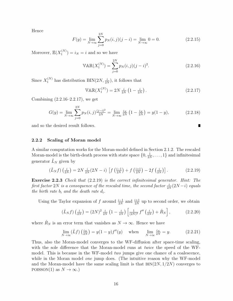
2.2.2 Scaling of Moran model
A similar computation works for the Moran-model defined in Section 2.1.2. The rescaledMoran-model is the birth-death process with state space 0, 1
2N, . . . , 1 and infinitesimal
generator LN given by
(LNf)(
i2N
)= 2N i
2N(2N − i)
[f(i−12N
)+ f
(i+12N
)− 2f
(i
2N
)]. (2.2.19)
Exercise 2.2.3 Check that (2.2.19) is the correct infinitesimal generator. Hint: Thefirst factor 2N is a consequence of the rescaled time, the second factor i
2N(2N−i) equals
the birth rate bi and the death rate di.
Using the Taylor expansion of f around i−12N
and i+12N
up to second order, we obtain
(LNf)(
i2N
)= (2N)2 i
2N
(1− i
2N
) [1
(2N)2 f′′ ( i
2N
)+ RN
], (2.2.20)
where RN is an error term that vanishes as N →∞. Hence we have
limN→∞
(Lf)(iN2N
)= y(1− y)f ′′(y) when lim
N→∞iN2N
= y. (2.2.21)
Thus, also the Moran-model converges to the WF-diffusion after space-time scaling,with the sole difference that the Moran-model runs at twice the speed of the WF-model. This is because in the WF-model two jumps give one chance of a coalescence,while in the Moran model one jump does. (The intuitive reason why the WF-modeland the Moran-model have the same scaling limit is that BIN(2N, 1/2N) converges toPOISSON(1) as N →∞.)
16

The fact that the WF-model and the Moran model have thesame space-time scaling limit is an example of what is calleduniversality. Biological systems that differ on a microscopicscale may have the same behavior on a macroscopic scale.
2.2.3 Wright-Fisher diffusion
The limiting process defined by (2.2.4) is called the Wright-Fisher diffusion. Think ofthis as a standard Brownian motion running at a “local speed” given by a diffusionfunction g : [0, 1]→ [0,∞), in our case g(y) = y(1− y) (see Fig. 5). Note that 0 and 1are traps: the WF-diffusion stops when it reaches the boundary of [0, 1] (a fact that isnot entirely trivial to prove).
0 1y
g(y)
Figure 5: Wright-Fisher diffusion function.
Returning to the h-version of the Moran-model mentioned at the end of Section 2.1.2,we find that the space-time scaling in (2.2.1) leads to the following.
Theorem 2.2.4 The h-version of the WF-diffusion satisfies the stochastic differentialequation
dYt =√Yt(1− Yt)h(Yt) dWt. (2.2.22)
Exercise 2.2.5 Give the proof of Theorem 2.2.4.
It is expedient to defineg(y) = y(1− y)h(y) (2.2.23)
and to write (2.2.22) as
dYt =√g(Y (t)) dWt. (2.2.24)
Here, g : [0, 1] → [0,∞) is the local diffusion function. In order for (2.2.24) to beproperly defined and have a unique strong solution, some restrictions have to be placedon g. We will return to this in Chapter 7.
17

2.3 Dual to WF-diffusion
The WF-diffusion describes the WF-model on large space-time scales. Even thoughthere is no easy explicit formula for Yt in terms of (Ws)0≤s≤t, (2.2.4) has the advantageof being easier to manipulate in computations than the original Markov chain. Toillustrate this advantage, we next turn to the notion of duality.
Theorem 2.3.1 Let D = (Dt)t≥0 be the death process on N = 1, 2, . . . where transi-tions from n to n− 1 occur at rate
(n2
). Then
E([Yt]n | Y0 = y) = E(yDt | D0 = n) ∀ y ∈ [0, 1], n ∈ N, t ≥ 0. (2.3.1)
Proof. Abbreviateat(y, n) = E([Yt]
n | Y0 = y),
bt(y, n) = E(yDt | D0 = n).(2.3.2)
Let f(x) = xn. Then it follows from (2.2.6) that (see Appendix A.2.1)
at(y, n)− a0(y, n) = E(f(Yt)− f(Y0) | Y0 = y)
= E(∫ t
0
(Lf)(Ys) ds | Y0 = y
)= E
(∫ t
0
Ys(1− Ys) 12f ′′(Ys) ds | Y0 = y
)= E
(∫ t
0
Ys(1− Ys) 12n(n− 1)[Ys]
n−2 ds | Y0 = y
)=
(n
2
)∫ t
0
[as(y, n− 1)− as(y, n)] ds.
(2.3.3)
Equation (2.3.3) is an integral recursion relation for at(y, n), which in differential formreads
∂
∂tat(y, n) =
(n
2
)[at(y, n− 1)− at(y, n)]. (2.3.4)
However, it follows from the definition of D that bt(y, n) satisfies the same recursion:
∂
∂tbt(y, n) =
(n
2
)[bt(y, n− 1)− bt(y, n)]. (2.3.5)
Exercise 2.3.2 Prove (2.3.5). Hint: Use the forward Chapman-Kolmogorov equationfor continuous-time Markov chains.
Sincea0(y, n) = yn = b0(y, n) ∀ y ∈ [0, 1], n ∈ N, (2.3.6)
it follows thatat(y, n) = bt(y, n) ∀ y ∈ [0, 1], n ∈ N, t ≥ 0, (2.3.7)
18

which proves the claim.
What Theorem 2.3.1 says is that the moments of Yt can be computed from thedistribution of Dt, and therefore so can the distribution of Yt itself. Since the dualprocess D is much simpler than the WF-diffusion Y , this constitutes a considerableadvantage. The following computation illustrates this advantage. We have
P(Y∞ = 1 | Y0 = y) = E(Y∞ | Y0 = y) = E(yD∞ | D0 = 1) = y, (2.3.8)
where we use (2.3.1) and the fact that Y∞ ∈ 0, 1 and D∞ = 1. This reflects the resultin Lemma 2.1.1. Similarly,
E(Yt(1− Yt) | Y0 = y) = E(yDt | D0 = 1)− E(yDt | D0 = 2)
= y −[y P(Dt = 1 | D0 = 2) + y2 P(Dt = 2 | D0 = 2)
]= y(1− y)P(Dt = 2 | D0 = 2)
= y(1− y)e−t,
(2.3.9)
where we use (2.3.1) together with the fact that Dt ∈ 1, 2 when D0 = 2 and Dt = 1when D0 = 1. This reflects the result in Lemma 2.1.2.
The dual process D can be traced back to the backward coalescing random walkencountered in the proof of Lemma 2.1.2. Indeed, Y describes the evolution of the typecomposition of a large population. Suppose that Y0 = y and we sample n individualsfrom this population at time t. The left-hand side of (2.3.1) is the probability to seeonly type A in the sample. But we can compute this probability differently. If we knowthat the n individuals in the sample are the descendants of Dt different ancestors attime 0, then by averaging over the random genealogy we obtain the right-hand side of(2.3.1) for the probability that all of the Dt ancestors are of type A.
More formally, consider the backward ancestral tree of a large population on thespace-time scale given by (2.2.1). Then
Dt = number of ancestral lineages at time t0 − t, t ∈ [0, t0], (2.3.10)
where t0 1 is any given observation time. In particular, D0 = 2N and Dt = 1 fort 1.
Theorem 2.3.3 The amount of time τk during which there are k lineages is equal tothe amount of time during which the death process D equals k, and has distributionEXP(λk) with λk =
(k2
), k ∈ N\1.
Proof. We first consider a sample of k individuals drawn from a WF-population offinite size 2N 1. Afterwards we make the proper space-time rescaling and let thepopulation size 2N tend to infinity.
The probability that two or more individuals from the sample have the same parentis
λk1
2N+O
(N−2
). (2.3.11)
19

Figure 6: Part of a backward ancestral tree of a population in the WF-diffusion. (Eachcontinuous unit of time corresponds to 2N discrete units of time.) In the death process timeis running upwards, while biological time is running downwards. The expectations of thetimes τ4, τ3 and τ2 equal, respectively, 1
6 , 13 and 1.
Indeed, there are λk different pairs of individuals in the sample, and in each pair thetwo individuals have the same parent with probability 1
2N. The first term takes into
account the event where precisely two individuals have the same parent, the secondterm takes into account events where there are two pairs of individuals who have thesame parents, or there are three or more individuals who all choose the same parent.
When we follow the ancestral lineages of the k individuals backwards in time (seeFig. 6), the probability that the k lineages do not coalesce during the first n generationsequals (
1− λk1
2N+O(N−2)
)n= exp
[−λk
n
2N+O(N−2)
]. (2.3.12)
Now rescale time by putting t = n/2N . Then in the limit as N → ∞ we have, for allt ≥ 0,
P(τk > t) = e−λkt. (2.3.13)
Thus, when the population size tends to infinity, τk has distribution EXP(λk), i.e., theexponential distribution with mean 1/λk.
3 Wright-Fisher: genealogy
In this chapter we take a closer look at the WF-model and the WF-diffusion backwardsin time. In Section 3.1 we make the duality encountered in Section 2.3 more transparantby introducing the Kingman coalescent, which is the time-reversed way of looking atthe WF-diffusion and provides information on the genealogy of the WF-model. In Sec-tion 3.2 we look at the most recent common ancestor of the population and investigate
20

how far back in time this ancestor lived. The presentation of the material in this chapteris taken from the bachelor thesis of Maurits Carsouw [4].
3.1 Kingman coalescent
Theorem 2.3.3 identifies the law of the random times of coalescence, but fails to capturethe genealogy, i.e., the tree structure of the population. A full description of all thelineages of the n individuals in the sample is achieved with the help of a coalescentprocess called the Kingman coalescent (see Kingman [16, 17]). This is a random processtaking values in the collection of partitions of 1, . . . , n such that, if the partition has jsets, then at rate 1
2j(j−1) two randomly chosen sets in the partition are joined together.
The Kingman coalescent, often called the coalescent, is a stochastic process thatdescribes the family tree of a large WF-population (2N 1) backwards in time, up tothe individual called most recent common ancestor (see Chapter 3.2). The coalescentis related to the WF-diffusion Y (see Section 2.2), and through duality to the deathprocess D (see Section 2.3). It is a powerful tool in the study of the genealogy of thepopulation up to the most recent common ancestor. Coalescent theory stands on itselfas an important area in population genetics (see Kingman [16], [17]).
In this section, the coalescent is constructed from the continuous-time Markov pro-cess called n-coalescent (Section 3.1.1). The transition probabilities and the absoluteprobabilities of this process will be calculated using the death process D. Existenceand uniqueness of the coalescent will be established by the Stone-Weierstrass theorem(Section 3.1.2). Finally, one of the coalescent’s most striking features is shown: it comesdown from infinity (Section 3.1.3).
3.1.1 n-coalescent
For n ∈ N, let En denote the set of partitions of the set 1, 2, . . . , n. The number ofsubsets in R ∈ En is denoted by |R|.
The n-coalescent is the continuous-time Markov process Rn = (Rnt )t≥0 with state
space En, initial stateRn
0 = ∆ = (1, 2, . . . , n), (3.1.1)
and transition ratesPRS = lim
h↓0h−1P(Rn
h = S | Rn0 = R) (3.1.2)
given by
PRS =
1, if S / R,0, otherwise,
R, S ∈ En, R 6= S, (3.1.3)
whereS / R⇔ S ∈ En : |S| = |R| − 1, (3.1.4)
i.e., S / R means that the partition S is obtained from the partition R by mergingtogether two of its subsets.
21

If we draw a sample of n individuals (from a large population) at time t0, then then-coalescent gives us a description of all the lineages of the n individuals backwards intime, i.e., the full tree structure (= genealogy). To understand this, let Rn
t denote thepartition such that i and j are in the same subset if and only if the individuals i and jhave a common ancestor that is alive at time t0 − t. With this definition, the processRn = (Rn
t )t≥0 indeed has the stochastic structure of an n-coalescent. Note that there isa one-to-one correspondence between the subsets in Rn
t and the common ancestors att0 − t involved in the sample.
Fig. 7 shows an example of the backward ancestral tree of a sample of size n = 4,taken (from a large population) at time t0. The jumps of the 4-coalescent are given by
R40 = (1, 2, 3, 4) = ∆,
R4t = (1, 2, 3, 4),
R4t+s = (1, 2, 3, 4),
R4t+s+v = (1, 2, 3, 4) = Θ.
(3.1.5)
Figure 7: Example of the backwards ancestral tree.
WriteDn = (Dnt )t≥0 for the natural restriction of the death processD = (Dt)t≥0 (defined
in Section 2.3) to the set 1, 2, . . . , n, so that Dn is the death process on 1, 2, . . . , nwith initial value Dn
0 = n and transitions from k to k − 1 that occur at rate λk =(k2
).
From (2.3.10) it is clear that Dnt equals the number of subsets in the partition Rn
t , i.e.,
Dnt = |Rn
t |. (3.1.6)
Indeed, each merger of Rnt corresponds to the extinction of one of the lineages in the
genealogy of the sample. Since Theorem 2.3.3 gives us the transition rates of D, itfollows from (3.1.6) that the total transition rate of Rn equals
PR =∑S∈En
PRS = limh↓0
h−1P(Rnh 6= R | Rn
0 = R) = λ|R|. (3.1.7)
Thus, the n-coalescent jumps with transition rates λk through a sequence of partitions<k with |<k| = k, k = n, n− 1, . . . , 1, such that
Θ = <1 / <2 / · · · / <n = ∆. (3.1.8)
22

The jump chain of the n-coalescent is defined as the Markov chain
(<n,<n−1, . . . ,<2,<1), (3.1.9)
which is directly related to its n-coalescent as
Rnt = <Dnt . (3.1.10)
From (3.1.3) and (3.1.7), we can now calculate the transition probabilities of the jumpchain. For R ∈ En with |R| = k ∈ 2, . . . , n, we have
P(<k−1 = S | <k = R) =PRSPR
=
1/λk, if S / R,0, otherwise.
(3.1.11)
Indeed, exactly one of the λk =(k2
)coalescence events turns R into S.
Finding the absolute probabilities of the jump chain requires a little more work (seeDurrett [10], Section 1.2.2, Theorem 1.5).
Theorem 3.1.1 For any R ∈ En with |R| = k,
P(<k = R) =k!
n!
(n− k)!(k − 1)!
(n− 1)!n1!× · · · × nk!, (3.1.12)
where n1, n2, . . . , nk are the sizes of the k subsets in R, satisfying n1 + ·+ nk = n.
Proof. We use induction on k, working backwards from k = n.
For k = n we have <k = <n = ∆, so that all subsets are of size 1,
n1 = . . . = nk = 1. (3.1.13)
Thus, we havek!
n!
(n− k)!(k − 1)!
(n− 1)!n1!× · · · × nk! = 1. (3.1.14)
Since R ∈ En with |R| = n implies that R = ∆, this is indeed equal to the statementthat
P(<n = R) = 1. (3.1.15)
Now, let k ∈ 2, . . . , n be arbitrary, and assume that the theorem holds for k (inductionhypothesis). We will prove that (3.1.12) also holds for k − 1.
Let S ∈ En with |S| = k − 1 and S / R. Then from (3.1.11) it follows that
P(<k−1 = S) =2
k(k − 1)
∑R : S/R
P(<k = R). (3.1.16)
Suppose that the subsets in S have sizes n1, . . . , nk−1. Then there exist l ∈ 1, . . . , k−1and m ∈ 1, . . . , nl − 1 such that the subsets in R have sizes
n1, . . . , nl−1,m, nl −m,nl+1, . . . , nk−1. (3.1.17)
23

From the induction hypothesis it follows that the right-hand side of (3.1.16) equals
2
k(k − 1)
k−1∑l=1
nl−1∑m=1
k!
n!
(n− k)!(k − 1)!
(n− 1)!
n1!× · · · × nl−1!m! (nl −m)!nl+1!× · · · × nk−1!
(nlm
)1
2.
(3.1.18)
Here,(nlm
)12
equals the number of ways to pick R with S / R so that the subsets in Rwith sizes m and nl −m coalesce to form the l-th subset in S with size nl. From thesimple fact that
n1!× · · · × nl−1!m! (nl −m)!nl+1!× · · · × nk−1!
(nlm
)= n1!× · · · × nk−1!, (3.1.19)
we conclude that the right-hand side of (3.1.18) equals
k!
n!
(n− k)!(k − 1)!
(n− 1)!n1!× · · · × nk−1!
1
k(k − 1)
k−1∑l=1
nl−1∑m=1
1
=k!
n!
(n− k)!(k − 1)!
(n− 1)!
(n− (k − 1))
k(k − 1)n1!× · · · × nk−1!
=(k − 1)!
n!
(n− (k − 1))!((k − 1)− 1)!
(n− 1)!n1!× · · · × nk−1!
(3.1.20)
and thus (3.1.12) indeed holds for k − 1.
3.1.2 Constructing the coalescent
We will now construct the coalescent from the n-coalescent (see also Kingman [16],Section 7). For 2 ≤ m < n, define the restriction ρnm : En → Em by dropping all thelabels m + 1, . . . , n from the subsets in the partitions making up En. If (Rn
t )t≥0 is then-coalescent, then (ρnmR
nt )t≥0 is the m-coalescent.
Let E denote the set of partitions of the set N, and define the restriction ρn : E → Enby dropping all the labels > n. We search for a process R = (Rt)t≥0 on E such that(ρnRt)t≥0 is the n-coalescent for all n ≥ 2. Such a process is called a coalescent. Thefollowing theorem justifies talking about the coalescent.
Theorem 3.1.2 There exists a unique coalescent R = (Rt)t≥0.
Proof. Note that E is a subset of the powerset 2N×N, and is a closed subset with respectto the (compact) product topology on 2N×N. When E is equipped with the subspacetopology, it becomes a compact Hausdorff space (a condition needed for the Stone-Weierstrass theorem below).
24

A coalescent exists when we can consistently specify its finite-dimensional distribu-tions. The consistency between different values of n is a consequence of the fact thatρnm(ρnS) = ρmS for all S ∈ E and 2 ≤ m < n. For fixed n, we consider the expectation
E(f(Rt1 , Rt2 , . . . , Rtk)
)(3.1.21)
for bounded continuous functions f : Ek → R and ordered times 0 ≤ t1 < t2 < . . . < tk.The requirement that (ρnRt)t≥0 is the n-coalescent determines the value of (3.1.21)when there exists a function g : (En)k → R such that f is of the form
f(S1, . . . , Sk) = g(ρnS1, . . . , ρnSk). (3.1.22)
The Stone-Weierstrass theorem implies that the set of functions f of this form is densein the set of bounded continuous functions f : Ek → R. Continuous extension thendetermines the value of (3.1.21) for all f , so that the consistent specification of thefinite-dimensional distributions is established. Since this is done uniquely, it followsthat any two coalescents have the same finite-dimensional distributions.
Exercise 3.1.3 Check the details of te proof.
With this definition, the coalescent R = (Rt)t≥0 is the Markov process on E withinitial condition R0 = (i : i ∈ N) such that each pair of subsets in Rt coalesces atrate 1 for all t ≥ 0. This means that every two lineages in the coalescent tree coalesceat rate 1 as we go backwards in time.
Where the n-coalescent gives a discription of the ancestral lineages of a sample of sizen taken from a large population, the coalescent gives a discription of all the lineagesof the whole population, up to the single individual from which the population hasdescended. In the WF-diffusion this population is assumed to be infinite. Thereforewe have to ask ourselves the question: How is it possible that the infinite number oflineages in the coalescent tree decreases to a finite number at positive times? Theanswer is provided in the next section: an entrance law can be used to describe how aMarkov process “comes down from infinity”.
3.1.3 Coming down from infinity
Now that we have familiarized ourselves with the construction of both the n-coalescentand the coalescent, we are ready to understand and prove an interesting phenomenon(see Berestycki [2], Section 2.1.2).
As before, we let Dt = |Rt| denote the number of subsets in Rt. Then we haveD0 =∞, which corresponds to the statement that there are infinitely many lineages atthe beginning of our coalescent tree. The following theorem says that after any positivetime we are left with only finitely many lineages. This is expressed by saying that thecoalescent comes down from infinity.
Theorem 3.1.4 P(∀ t > 0: Dt <∞) = 1.
25

Proof. We must show that
∀ t > 0 ∀ ε > 0 ∃Nt,ε ∈ N : P(Dt > Nt,ε) < ε. (3.1.23)
Let t > 0 and ε > 0 be arbitrary. Furthermore, let Rnt = ρn(Rt) be the natural
restriction of the coalescent to En, and let Dnt = |Rn
t | denote the number of subsetsin Rn
t . Let τk be the random variable with distribution EXP(λk), k ∈ N\1. ThenTheorem 2.3.3 says that we can use τk to represent the amount of time during whichDt = k. Therefore, using the Markov inequality, we have
P(Dnt > Nt,ε) = P
n∑k=Nt,ε
τk > t
≤ 1
tE
n∑k=Nt,ε
τk
≤ 1
t
∞∑k=Nt,ε
E(τk) =1
t
∞∑k=Nt,ε
1
λk,
(3.1.24)
where we note that the last sum is independent of n. Since∑
k∈N 1/λk < ∞, we canchoose Nt,ε large enough to make sure that
1
t
∞∑k=Nt,ε
1
λk
< ε, (3.1.25)
from which it follows that
lim supn→∞
P(Dnt > Nt,ε) = lim
n→∞
(supm≥n
P(Dmt > Nt,ε)
)< ε, (3.1.26)
which is (3.1.23).
The Kingman coalescent describes the genealogy of the WF-population inthe space-time scaling limit. It is a universal process, in the sense that otherpopulations like the Moran-population have the same limit.
3.2 Most recent common ancestor
An object of interest in population genetics, in particular, in coalescent theory, is themost recent common ancestor (MRCA). Consider a population where all individualshave a common allele (or locus, or gene). We can trace this allele in the ancestry of thepopulation. As we move backwards in time, the collection of ancestors shrinks, untilwe are left with the single individual from which the whole population has descended.This individual is found at the root of the coalescent tree, and is called the MRCA. Itis the most recent individual that is a common ancestor of the whole population.
In this section we investigate the MRCA of a population in the WF-diffusion. Thecoalescent enables us to calculate the expectation of the time between the population
26

and its MRCA (Section 3.2.1). As time runs forward, the MRCA jumps forward inorder to keep up with the population. This jump process is called the MRCA-process,which we will analyze in Appendix B by means of a “particle construction” introducedby Donnelly and Kurtz [9]. In particular, we will determine the distribution of thewaiting time between the successive jumps in the MRCA-process (Section 3.2.2).
3.2.1 Depth of the coalescent tree
Consider a population in the WF-diffusion where every individual is of type A or oftype a. If the population has a MRCA, then this MRCA is either of type A or of typea, from which it follows that the whole population is either of type A or of type a.The reverse does not necessarily hold: if a population descends for example from twoindividuals instead of one, and these two individuals are both of the same type, thenthe whole population is of one type, but does not have a MRCA.
Suppose that the WF-diffusion has been running indefinitely, and observe a popu-lation in the WF-diffusion at some reference time t0 ∈ R. Then this population has aMRCA a.s. (i.e., the MRCA did not live an infinite amount of time ago). In fact, giventhe time at which the population lives, we can predict the time of its MRCA.
Theorem 3.2.1 Let T be the time between the population in the WF-diffusion and itsMRCA. Then E(T ) = 2.
Proof. Let τk be the amount of time during which there are k lineages in the coalescenttree of the population, k ∈ N\1. Then Theorem 2.3.3 states that E(τk) = 1/λk =1/(k2
). Since the time between the population and its MRCA equals the depth of the
coalescent tree, the desired expectation equals
E(T ) = E
(∞∑k=2
τk
)=∞∑k=2
E(τk) =∞∑k=2
2
k(k − 1)= 2. (3.2.1)
Remark: Theorem 3.2.1 is stated in terms of a continuous rescaled time. For example,if we use the WF-diffusion to approximate the behaviour of a population of size 2N =50, 000, then according to the space-time rescaling in (2.2.1), we expect that the MRCAlives 50, 000× 2 = 100, 000 generations (discrete-time units) ago.
The average time to the most recent common ancestor is twice thepopulation size.
3.2.2 MRCA-process and F-process
Let t ∈ R be the observation time of a population in the WF-diffusion, and let Tt bethe depth of the corresponding coalescent tree. Then At = t− Tt is the time at which
27

the MRCA of the time-t population lives. We define the MRCA-process as the process(At)t∈R on state space R. (Donnelly and Kurtz [9] refer to (At)t∈R as the “Eve process”).
Consider the MRCA that lived at timeAt, and the two individuals directly descendedfrom this MRCA. The time-t population is then divided into two disjoint parts, whereeach part consists of the time-t offspring of one of the two individuals. We refer to theseparts as the two oldest families in the population. The time Ft at which one of thesefamilies fixates in the population, a new MRCA is established. The process (Ft)t∈R onstate space R is called the F-process.
Suppose that the points of (At)t∈R are enumerated as αii∈Z. Then the pointsβii∈Z of (Ft)t∈R are given by βi = inft ∈ R : At = αi (see Fig. 8), and the path of(At)t∈R is constant on each interval [βi, βi+1):
∀ t ∈ [βi, βi+1) : At = αi. (3.2.2)
In this way, at each time βi the MRCA, which lives at time αi, is established.
Figure 8: Time is running horizontally to the right. The time points αj and βj , i− 2 ≤ j ≤i+ 2, of the MRCA-process (At)t∈R and the F-process (Ft)t∈R are drawn for fixed i ∈ Z. Thedotted lines relate each time αj at which a MRCA lives to the time βj at which this MRCAis established.
In Appendix B we will prove the following two theorems (see Appendix A.2.2).
Theorem 3.2.2 The MRCA-process (At)t∈R is a rate-1 Poisson process on R.
Theorem 3.2.3 The F-process (Ft)t∈R is a rate-1 Poisson process on R.
Successive MRCA’s in the WF-diffusion occur at Poisson times.The average time between successive MRCA’s is 1.
Exercise 3.2.4 In Theorem 3.2.1 we saw that the average time between the populationand its MRCA is 2. Is there a paradox because 1 6= 2?
4 Wright-Fisher with mutation
In this chapter we add mutation. In Section 4.1 we look at the standard model withtwo types, in Sections 4.2–4.3 at the model with infinitely many types, respectively,with infinitely many sites (= base pairs).
28

4.1 Wright-Fisher with mutation and two types
4.1.1 Mutation
Suppose that we modify the WF-model in the following manner. At each time uniteach individual, immediately after it has chosen its ancestor and adopted its type (re-sampling), suffers a type mutation: type a spontaneously mutates into type A withprobability u, and type A spontaneously mutates into type a with probability v (seeFig. 9). Here, 0 < u, v < 1, and mutations occur independently for different individuals.
An alternative way to include the mutation is to say that, after the resampling,each individual mutates into type A or a with probability u, respectively, v irrespectiveof its type. Since the transitions A → A and a → a do not effect the population,this type-independent mutation gives the same model, but is easier to work with (seebelow).
a A
u
v
t t
Figure 9: Two-type mutation.
Our goal is to investigate what effect the mutation has on the behavior of the model.With mutation X = (Xn)n∈N0 is a Markov chain on the state space Ω with transitionkernel
p(i, j) =
(2N
j
)(pi)
j(1− pi)2N−j, i, j ∈ Ω, (4.1.1)
with
pi =
(i
2N
)(1− v) +
(2N − i
2N
)u. (4.1.2)
Indeed, either an A is drawn (probability i2N
) and it does not mutate into an a (probabil-ity 1−v), or an a is drawn (probability 2N−i
2N) and it does mutate into an A (probability
u). Compare (4.1.1–4.1.2) with (2.1.2).
A first consequence of the presence of mutation is that the traps at 0 and 2Ndisappear: p(i, j) > 0 for all i, j ∈ Ω.
Due to mutation there no longer is loss of genetic variability!
In fact, because N is finite, we have w − limn→∞Xn = X with
π(i) = P(X = i), i ∈ Ω, (4.1.3)
29

an equilibrium distribution solving the set of equations∑i∈Ω
π(i)p(i, j) = π(j), j ∈ Ω, (4.1.4)
normalized such that∑
i∈Ω π(i) = 1. The equilibrium has full support, i.e., π(i) > 0 forall i ∈ Ω. In principle it is possible to compute π, but the formulas are not so pretty.We get some insight by computing the first two moments of X.
Lemma 4.1.1 The first and second moment of X are given by
E(X
2N
)= ρ,
E(
X(X − 1)
2N(2N − 1)
)= χρ+ (1− χ)ρ2,
(4.1.5)
where
ρ =u
u+ v, χ =
(1− µ)2
(1− µ)2 + 2N [1− (1− µ)2], µ = 1− (1− u)(1− v). (4.1.6)
Proof. Suppose that the system is in equilibrium. Let ηi = 1 if the i-th individual is Aand ηi = 0 otherwise. Then
X =2N∑i=1
ηi, (4.1.7)
and, by exchangeability,
E(X) = 2NP(η1 = 1),
E(X(X − 1)) = 2N(2N − 1)P(η1 = η2 = 1).(4.1.8)
To compute the first probability in (4.1.8), abbreviate ρ = P(η1 = 1). In equilibriumwe have
ρ = (1− v)ρ+ u(1− ρ). (4.1.9)
This gives ρ = uu+v
and proves the first line of (4.1.5). To compute the second probabilityin (4.1.8), note that in equilibrium
P(η1 = η2 = 1) = χρ+ (1− χ)ρ2, (4.1.10)
where
χ = the probability that two individuals are identical by descent,
i.e., their lineages coalesce before a mutation affects either lineage.(4.1.11)
To compute χ we argue as follows. Let µ = 1 − (1 − u)(1 − v) be the probability ofmutation per unit of time backwards on a lineage. Then the probability 1−χ that twoindividuals are not identical by descent satisfies the equation
1− χ = [1− (1− µ)2] + (1− µ)2
(1− 1
2N
)(1− χ). (4.1.12)
30

Indeed, if at the first time step backwards there is no mutation in either of the twolineages (probability (1−µ)2) nor coalescence of the two lineages (probability 1
2N), then
“the game starts all over again”. Solving (4.1.12) for χ and inserting into (4.1.8), wefind the second line of (4.1.5).
An interesting consequence of Lemma 4.1.1 is that
limN→∞
X
2N= ρ in probability. (4.1.13)
In large populations with mutation the fraction of types is closeto a deterministic value.
In Section 4.1.2 we will see that the limit is random when u, v tend to zero as N →∞in an appropriate manner.
Remark: In the presence of mutation, the coalescent (= the backward tree of lineages)modifies in the following manner. At each unit of backward time, a backward path: (i)is killed and labelled A with probability u; (ii) is killed and labelled a with probabilityv; (iii) jumps to a randomly chosen parent with probability (1− u)(1− v); and (i)–(iii)occur independently). Killing a path determines the state of all its descendants (seeFig. 10). Note that if all the backward paths are killed, then the state of the system nolonger depends on the initial configuration. This is why the system reaches equilibriumin the presence of mutation.
r rr
r
A
a
a
A
A
a
a
A
A
a
A
a
Figure 10: The coalescent with mutation in equilibrium. Time for the coalescent runs to theright (which means that biological time runs to the left). The black dots denote killing dueto mutation, at which moment type A or type a is chosen with probability u, respectively, vand the rest of the coalescent is removed. After the A’s and the a’s have been assigned at theblack dots, the states of the descendants are determined.
31

4.1.2 Weak mutation
Interesting behavior shows up in the limit as N → ∞, provided we take the mutationprobabilities small:
u = u(N) =q
4N, v = v(N) =
r
4N, q, r > 0. (4.1.14)
The reason behind this choice is apparent from Lemma 4.1.1: for u, v ↓ 0 we haveµ ≈ (u + v) and χ ≈ 1/(1 + 4N(u + v)), which shows that 4N(u + v) is the relevantquantity for the scaling behavior. Think of 1
2q, 1
2r as the mutation rates of the whole
population.
Remark: The reason why we divide by 4N rather than 2N in (4.1.14) is a matter ofconvention. In the Moran-model, which for large N runs at twice the speed of the WF-model (recall Section 2.2.2), we must divide by 2N to get the correct correspondence.
Define, in analogy with (2.2.1),
Y (N) =1
2NX(N). (4.1.15)
Then we expect thatw − lim
N→∞Y (N) = Y. (4.1.16)
Theorem 4.1.2 The convergence in (4.1.16) is true, with Y the random variable on[0, 1] with distribution BETA(q, r), i.e., with probability density
f(x) = Cq,rxq−1(1− x)r−1, x ∈ [0, 1], (4.1.17)
where Cq,r = Γ(q+r)/Γ(q)Γ(r) is the normalizing constant ( Γ is the Gamma-function).
Proof. The proof is by brute force and proceeds via a computation of the moments ofY . We will show that
E(Y k) = mk, mk =
∏k−1j=0(q + j)∏k−1
j=0(q + r + j), k ∈ N, (4.1.18)
which are the moments of BETA(q, r). The computation of mk is by induction, namely,we will show that
mk =q + k − 1
q + r + k − 1mk−1, k ∈ N, m0 = 1. (4.1.19)
Given that X(N)n−1 = i, the distribution of X
(N)n is BIN(2N, pi). Therefore
E
(k−1∏j=0
(X(N)n − j)
∣∣∣ X(N)n−1 = i
)=
(k−1∏j=0
(2N − j)
)(pi)
k. (4.1.20)
32

Dividing by (2N)k, expanding to leading order in 12N
and putting Y(N)n = 1
2NX
(N)n , we
may rewrite this equation as
E([Y (N)n
]k | Y (N)n−1 = 2Ni
)− k(k − 1)
4NE([Y (N)n
]k−1 | Y (N)n−1 = 2Ni
)+O
(1
N2
)=
[1− k(k − 1)
4N+O
(1
N2
)](pi)
k,
(4.1.21)where we use that
∑k−1j=0 j = 1
2k(k − 1). Next, we expand
(pi)k =
(i
2N(1− u− v) + u
)k=
(i
2N
)k+ k
(i
2N
)k−1 [q
4N−(
i
2N
)q + r
4N+O
(1
N2
)],
(4.1.22)
where we use (4.1.2) and (4.1.14). Combining (4.1.21–4.1.22), we get
E([Y (N)n
]k | Y (N)n−1
)− k(k − 1)
4NE([Y (N)n
]k−1 | Y (N)n−1
)+O
(1
N2
)=
[1− k(k − 1)
4N+O
(1
N2
)]×[Y
(N)n−1
]k+ k
[Y
(N)n−1
]k−1[q
4N−[Y
(N)n−1
] q + r
4N+O
(1
N2
)].
(4.1.23)
Taking the expectation over Y(N)n−1 , letting n → ∞ and using that w − limn→∞ Y
(N)n =
Y (N), we obtain the relation
k(k + q + r − 1)
4NE([Y (N)]k) =
k(k + q − 1)
4NE([Y (N)]k−1) +O
(1
N2
). (4.1.24)
Finally, multiplying by 4N/k, letting N → ∞ and using that limN→∞ Y(N) = Y , we
obtain (4.1.19).
Exercise 4.1.3 Prove Theorem 4.1.2 with the help of convergence of generators, as inSection 2.2.
The qualitative behavior of the probability density in (4.1.17) near the boundaries0 and 1 is different for q, r < 1 and q, r > 1 (see Fig. 11).
The shape of the limiting distribution for the fractions of the typesin a large population provides information on the mutation rates.
In the limit as q, r ↓ 0, f concentrates on the boundaries, in accordance with theeventual loss of genetic variability in the WF-model without mutation (or rather inthe WF-diffusion, because we took the limit N → ∞). In the limit as q, r → ∞, fconcentrates around the value q
q+r, in accordance with what we found in (4.1.13).
33

f(x)
0 1
f(x)
0 1
Figure 11: Qualitative picture of the probability density in (4.1.17) for q, r < 1 and q, r > 1,respectively.
4.2 Wright-Fisher with mutation and infinitely many types
In this section we consider the modification of the WF-model in which, instead of twotypes, there are infinitely many types and each time a mutation occurs it brings in anew type. The motivation for this model is the following. If a gene consists of, say, 500nucleotides, then there are 3 × 500 = 1500 sequences that can be reached by a singlebase pair change. Therefore the probability of returning to the same sequence aftertwo mutations is 1/1500, which is small. Neglecting this return amounts to consideringwhat is called the infinite alleles model.
In Section 4.2.1 we define the model, show that it is dual to a birth process calledthe Hoppe urn model, and use the latter to study the distribution of the number ofdifferent types in an n-sample of individuals drawn randomly from the population. InSection 4.2.2 we use the Hoppe urn model to derive the Ewen sampling formula, whichdescribes the sizes of the families of different types in the n-sample. In Section 4.2.3 welook at the sizes of these families in the limit as n→∞.
4.2.1 Infinite alleles model
Types are labelled 0, 1, 2, . . .. We consider a population with 2N individuals, all startingwith type 0. At each unit of time, each individual with probability 1 − µ chooses arandom ancestor and adopts its type and with probability µ spontaneously mutates intoa new type. All individuals update independently from each other and independentlyof how they updated at previous times. The first mutation in the population brings inan individual of type 1, the second an individual of type 2, etc. As time proceeds, newtypes enter the population and old types die out. However, we may expect that aftera long time the distribution of the number of different types in the population settlesdown to a limiting distribution. The question we want to address is: “What is thisdistribution?”.
Remark: The infinite alleles model was proposed by Kimura in 1968. At that time itwas not yet possible to sequence the genome, so the precise order of the nucleotides inan allele, which determines its type, could not yet be determined. However, with thehelp of e.g. electrophoresis of enzymes it was possible to distinguish between differenttypes, and so the number of different types could be measured.
34

We will consider this question in the limit as N →∞, with
µ = µ(N) =θ
4N, θ > 0, (4.2.1)
where 12θ may be thought of as the mutation rate for the whole population. In this limit,
after time is scaled by a factor 2N as well (recall (2.2.1)), we have that
k lineages coalesce at rate λk =
(k
2
)and mutate at rate 1
2θk. (4.2.2)
(Use that BIN(2N, θ/4N) converges to POISSON(12θ) as N →∞.)
Draw a random sample of n individuals from the population in equilibrium (n N →∞) and ask for
Kn = the number of different types in the n sample. (4.2.3)
Lemma 4.2.1 As n→∞,E(Kn) ∼ θ log n,
VAR(Kn) ∼ θ log n.(4.2.4)
Moreover, the central limit holds, i.e., w−limn→∞[Kn−E(Kn)]/√
VAR(KN) = N(0, 1),the standard normal distribution.
Proof. The proof uses duality. The dual process is called the Hoppe urn model, whichis defined as follows:
• An urn contains 1 black ball (of mass θ) and any number of colored balls (of mass1 each). A ball is selected with a probability proportional to its mass. If a coloredball is drawn, then an extra ball with the same color is put into the urn. If theblack ball is drawn, then an extra ball with a new color is put into the urn. Theball that was drawn is put back into the urn also.
We start with 1 black ball at time 0. At time n the urn contains n+1 balls, 1 black andn colored. The state of the urn is the number of different colors and their multiplicity.The key observation is the following duality :
• The genealogy of n individuals in the infinite alleles model can be simulated byrunning the Hoppe urn model for n time steps.
Indeed, the genealogy of the infinite alleles model is described by a coalescent with killingsimilar in spirit as the one in Fig. 10 (recall (4.2.2)): (i) lineages change randomly andwhen they meet coalesce at rate 1; (ii) on each lineage there is an independent Poissonprocess with rate 1
2θ of mutations that kill the lineage and determine the type of all the
decendants. See Durrett [10], Figure 1.7. A draw of the black ball signals a mutationin the backwards genealogy.
35

Exercise 4.2.2 Check the above duality. Hint: the probability to mutate in the infinitealleles model when there are k lineages equals k 1
2θ/[k 1
2θ + 1
2k(k − 1)] = θ/[θ + k − 1],
which is precisely the probability in the Hoppe urn model to bring in a new color at thek-th draw.
What is nice about the Hoppe urn model is that it is a simple process, controlledby the parameter θ, and that it simulates all sample sizes at once: the sample size n inthe infinite alleles model is the number of draws in the Hoppe urn model.
With the above duality the proof of (4.2.4) is easy. Write
Kn =n∑i=1
ηi (4.2.5)
with ηi = 1 if the i-th ball added in the Hoppe urn model has a new color and zerootherwise. Clearly, the successive ηi are independent (because at time i the urn alwayscontains i+ 1 balls, one with mass θ and i with mass 1), and
P(ηi = 1) =θ
θ + i− 1. (4.2.6)
Consequently,
E(Kn) =n∑i=1
P(ηi = 1) =n∑i=1
θ
θ + i− 1
∼ θ
∫ θ+n
θ
dx
x= θ[log(θ + n)− log θ] ∼ θ log n.
(4.2.7)
Similarly,
VAR(Kn) =n∑i=1
VAR(ηi) =n∑i=1
θ
θ + i− 1
(1− θ
θ + i− 1
)∼ E(Kn). (4.2.8)
This proves (4.2.4). The central limit theorem follows from standard arguments.
Exercise 4.2.3 What are the conditions in the central limit theorem for sums of inde-pendent random variables (not necessarily identically distributed)? Do these conditionsapply to (4.2.5)? Hint: Consult a standard probability textbook.
Lemma 4.2.1 says that the number of different types in an n sample is rather small,namely, of order log n. Apparently, new types rapidly eradicate old types, so that it ishard for different types to coexist in large numbers.
The number of different types is proportional to θ. Hence θ can beestimated from genetic sample data, which is interesting becausetypically θ is not known.
Lemma 4.2.1 shows that θn = Kn/ log n is an asymptotically sharp estimator of θ (“asufficient statistic”). Unfortunately, the standard deviation of θn decays like 1/
√log n,
which is too slow to get sharp estimates unless n is very large. Still, θ can be used toestimate θ with some confidence interval.
36

4.2.2 Ewens sampling formula
The next result, which is referred to as Ewens sampling formula, describes the fullfamily size distribution of the types in the n-sample. Let
Ai = the number of types that are present precisely i times in the n-sample,
i = 1, . . . , n,(4.2.9)
and note that∑n
i=1 iAi = n. This is the “type frequency spectrum” of the n-sample.E.g. (n, 0, . . . , 0) corresponds to n types each being present once, while (0, . . . , 0, 1)corresponds to one type being present n times. In particular, Kn =
∑ni=1Ai, which
establishes the link with Section 4.2.1.
Write A = (Ai)ni=1, let
An =
a = (ai)
ni=1 :
n∑i=1
iai = n
, n ∈ N, (4.2.10)
and abbreviate Pn(a) = P(A = a), a ∈ An.
Theorem 4.2.4 For all n ∈ N and a ∈ An,
Pn(a) = n!n∏i=1
(θ/i)ai
(θ + i− 1)ai!. (4.2.11)
Proof. We will again make use of the duality with the Hoppe urn model. The proof isby induction on n. If n = 1, then a = (a1) = (1), and the claim in (4.2.11) is true withP1(1) = 1.
Pick n ≥ 2. For a′ ∈ An−1 and a ∈ An, let p(a′, a) denote the transition probabilityfrom state a′ at time n − 1 to state a at time n in the Hoppe urn model. Let Pn(a)denote the right-hand side of (4.2.11). We will show that
Pn(a) =∑
a′∈An−1
Pn−1(a′)p(a′, a) ∀ a ∈ An, (4.2.12)
which will imply that Pn is the distribution of the Hoppe urn model at time n, i.e.,Pn = Pn, and will complete the proof by induction.
Suppose that the state at time n− 1 is a′ and the state at time n is a. Then thereare two possibilities:
(1) a1 = a′1 + 1, ai = a′i for i > 1, i.e., a new color is added at time n. For this case
Pn(a)
Pn−1(a′)=
n
θ + n− 1
θ
a1
, p(a′, a) =θ
θ + n− 1. (4.2.13)
37

(2) aj = a′j − 1, aj+1 = a′j+1 + 1, ai = a′i for 1 ≤ j ≤ n − 1 and i 6= j, j + 1, i.e., acolor is added at time n that is present j times at time n− 1. For this case
Pn(a)
Pn−1(a′)=
n
θ + n− 1
ja′j(j + 1)aj+1
, p(a′, a) =ja′j
θ + n− 1. (4.2.14)
No other transitions are possible. From (4.2.13–4.2.14) we get
∑a′∈An−1
Pn−1(a′)
Pn(a)p(a′, a)
=θ + n− 1
n
a1
θ
θ
θ + n− 1+
n−1∑j=1
θ + n− 1
n
(j + 1)aj+1
ja′j
ja′jθ + n− 1
=a1
n+
n−1∑j=1
(j + 1)aj+1
n
=1
n
n−1∑j=0
(j + 1)aj+1 = 1,
(4.2.15)
which shows that indeed (4.2.12) is true.
Remark: A more intuitive proof can be found in Griffiths and Lessard [13].
The Ewens sampling formula not only provides insight into thefamily size distribution of the types in an n-sample, it also allowsfor a more sophisticated way of statistically estimating θ.
By rewriting (4.2.11) as
Pn(a) =1
Nθ,n
n∏i=1
e−θ/i(θ/i)ai
ai!, a ∈ An, (4.2.16)
with Nθ,n the normalizing constant, we see that Pn can be interpreted as the distributionof a random vector (A1, . . . , An) whose components Ai are independent and Poissondistributed with mean θ/i conditioned on
∑ni=1 iAi = n.
Small frequencies are more likely than large frequencies. The reason isthat if a type does not appear in the n-sample so often, then it is lesslikely to reduce in number by mutation.
38

4.2.3 GEM-distribution
The next result describes the behavior of the Ewens sampling formula in the limit asn→∞. Let us call the descendants of the k-th new color in the Hoppe urn model thek-th family. This is the collection of all the balls in the urn that carry color k. Let
Sk(n) =1
n× the size of the k-th family at time n. (4.2.17)
Consider the random vector
S(n) = (Sk(n) : k ∈ N). (4.2.18)
Note that the components of this vector sum up to 1 (and are 0 in the tail).
Theorem 4.2.5 w− limn→∞ S(n) = B with B = (Bk : k ∈ N) the random vector givenby
Bk =
[k−1∏j=1
(1− Zj)
]Zk, k ∈ N, (4.2.19)
where (Zk)k∈N are i.i.d. with distribution BETA(1, θ), i.e., with probability density func-tion f(z) = θ(1− z)θ−1, z ∈ [0, 1].
Proof. We make use of the following observation, relating the Hoppe urn model to abranching process with immigration:
• Immigrants enter the population at the times of a Poisson process with rate θ.Each individual performs a binary branching process, i.e., splits into two at rate1 (= gives birth to a new individual at rate 1 and does not die).
The key observation is:
• Start with 1 immigrant entering at time 0. If each immigrant is a new type andoffspring are the same type as their parents, then the successive states of thebranching process with immigration have the same distribution as the successivestates of the Hoppe urn model.
What is done here is that the Hoppe urn model (discrete in time) is embedded into thebranching process with immigration (continuous in time). (In the Hoppe urn model, nis the number of colored balls in the urn and Sk(n) is the fraction of colored balls withcolor k.)
Exercise 4.2.6 Prove the above embedding.
Armed with these observations we argue as follows. Let X(t) be the number ofindividuals at time t in the branching process without immigration. Then it is wellknown that E(X(t)) = et, t ≥ 0, and
w − limt→∞
e−tX(t) = E = EXP(1). (4.2.20)
39

Exercise 4.2.7 Look up the proof of (4.2.20) (see Durrett [10], Section 1.3.3).
Let Xk(t) be the number of individuals in the k-th family at time t in the branchingprocess with immigration. Then (4.2.20) implies that
w − limt→∞
(e−tXk(t) : k ∈ N) = (e−TkEk : k ∈ N), (4.2.21)
where Ek, k ∈ N, are i.i.d. copies of E and Tk, k ∈ N are the successive arrival timesof an independent Poisson process with rate θ (= the immigration times). Here we usethat the branching process with immigration is the independent sum of the branchingprocesses without immigration starting at the successive arrival times of the immigrants.Let
I(t) =∑k∈N
Xk(t) (4.2.22)
be the total number of individuals at time t, and let
σ =∑k∈N
e−TkEk. (4.2.23)
Then (4.2.21) givesw − lim
t→∞e−tI(t) = σ. (4.2.24)
It follows from (4.2.21–4.2.24) that the limit Bk we are after in (4.2.19) arises as
Bk = w − limt→∞
Xk(t)
I(t)=e−TkEkσ
, k ∈ N, (4.2.25)
where we use the embedding of the Hoppe urn model into the branching process withimmigration. To identify the distribution of (Bk : k ∈ N), we define (T0 = 0)
σj =∞∑k=j
e−(Tk−Tj−1)Ek, j ∈ N,
Zj =Ej
Ej+σj+1, j ∈ N,
(4.2.26)
and note that σ1 = σ. For k = 1, write
B1 =e−T1E1
σ1
=e−T1E1
e−T1(E1 + σ2)=
E1
E1 + σ2
= Z1. (4.2.27)
For k = 2, write
B2 =e−T2E2
σ1
=e−T2E2
e−T1(E1 + σ2)=
σ2
E1 + σ2
e−(T2−T1)E2
σ2
=σ2
E1 + σ2
e−(T2−T1)E2
e−(T2−T1)(E2 + σ3)=
σ2
E1 + σ2
E2
E2 + σ3
= (1− Z1)Z2.
(4.2.28)
Exercise 4.2.8 Give the proof of (4.2.19) by induction on k. Use (4.2.27–4.2.28).
40

It remains to show that (Zj)j∈N has the desired distribution. Recall the notation inAppendix A.2.1 and abbreviate GAMMA(θ, 1) = GAMMA(θ), θ ∈ (0,∞).
Lemma 4.2.9 σ has distribution GAMMA(θ).
Proof. Since (Ej, Tj−Tj−1), j ∈ N, are i.i.d. with distribution EXP(1)×EXP(θ), we havethat
∑j∈N δEj ,Tj is the Poisson point process on [0,∞)× [0,∞) with intensity measure
θdx ⊗ e−ydy. Consequently,∑
j∈N δe−Tj Ej is the Poisson point process on [0,∞) with
intensity measure e−z θdzz
. Indeed, for any test function f : (0,∞) → [0,∞) that iscontinuous and has compact support, we have∫ ∞
0
∫ ∞0
θdx e−ydy f(e−xy) =
∫ ∞0
e−ydy
∫ y
0
θdz
zf(z)
=
∫ ∞0
f(z)θdz
z
∫ ∞z
e−ydy =
∫ ∞0
f(z) e−zθdz
z.
(4.2.29)
Since e−z θdzz
is the Levy measure of the Gamma-process (see Bertion [3]), the claimfollows.
Lemma 4.2.10 (Zj), j ∈ N, are i.i.d. with distribution BETA(1, θ).
Proof. We will need the following property of the Gamma-distribution (L denotes law):
L[(G1, G2)] = GAMMA(θ1)⊗ GAMMA(θ2)
=⇒ L[(G1 +G2,
G1
G1 +G2
)]= GAMMA(θ1 + θ2)⊗ BETA(θ1, θ2).
(4.2.30)
Exercise 4.2.11 Write out the proof.
Abbreviate Wj = Ej + σj+1. We use (4.2.30) to show that
L[(W1, Z1, . . . , Zn)] = GAMMA(1 + θ)⊗ BETA(1, θ)⊗n, n ∈ N, (4.2.31)
which will prove the claim.
First, we check that (4.2.31) is true for n = 1. Indeed,
W1 = E1 + σ2, Z1 =E1
E1 + σ2
. (4.2.32)
By Lemma 4.2.9, L[σ2] = L[σ] = GAMMA(θ), because the distribution of (σj)j∈N isshift-invariant. Since L[E1] = EXP(1) = GAMMA(1) and E1 is independent of σ2 (recall(4.2.26)), (4.2.30) and (4.2.32) yield
L[(W1, Z1)] = GAMMA(1 + θ)⊗ BETA(1, θ). (4.2.33)
41

Next, we suppose that (4.2.31) is true for n. Then, since the distribution of (Ej, Tj−Tj−1)j∈N is shift-invariant, we have (recall (4.2.26))
L[(W2, Z2, . . . , Zn+1)] = GAMMA(1 + θ)⊗ BETA(1, θ)⊗n. (4.2.34)
But (W2, Z2, . . . , Zn+1) is independent of (E1, T2−T1) and, since W1 = E1 +e−(T2−T1)W2,also independent of (W1, Z1) conditional on W2. Therefore, combining (4.2.33–4.2.34),we conclude that (4.2.31) is true for n + 1 aslo. Hence, by induction on n, it followsthat (4.2.31) holds for all n ∈ N.
Exercise 4.2.8 and Lemma 4.2.10 complete the proof of Theorem 4.2.5.
The limiting distribution in Theorem 4.2.5 is called the Griffiths, Engen, McCloskeydistribution (GEM).
The GEM distribution describes the frequency spectrum of thetypes in a very large sample in the age order, i.e., the types areordered according to their first appearance. It has a “random stickbreaking” structure.
4.3 Wright-Fisher with mutation and infinitely many sites
In the infinite alleles model in Section 3.2 we only kept track of when sequences becamedifferent through mutation and referred to these differences as a change of type. Wedid not keep track of the number of differences between the sequences. In the presentsection we will introduce a model, called the infinite sites model, that keeps track ofwhere in the sequence the mutations occur and we will count these mutations.
Given are two genes of length L. Think of these as a sample of size n = 2 drawnfrom a population with 2N genes (= individuals), each having a type that is given byits sequence of nucleotides of length L. Let ∆2 be the number of pairwise differencesin the two sequences. An example with L = 14 is
AATCGCTTGATACCACTCGCCTGATAAC
which has pairwise differences at positions 2, 7 and 13, so that ∆2 = 3. Let µ = µ(N) =θ/4N be the mutation rate as in (4.2.1). We are interested in the distribution of ∆2
in the limit as N → ∞ and L → ∞. The latter limit is the reason why the model iscalled the infinite sites model.
Lemma 4.3.1 ∆2 has distribution GEO(1/(θ + 1)), i.e.,
P(∆2 = k) =1
θ + 1
(θ
θ + 1
)k, k ∈ N0. (4.3.1)
42

Proof. In the limit as L→∞, mutations always occur at different sites and so we mayuse the duality with the Hoppe urn model. As we saw in Section 4.2.1, in the limitas N → ∞, with time multiplied by 2N , two lineages mutate at rate 2µ(N)2N =θ and coalesce at rate 1
2N2N = 1. Therefore the probability of coalescence before
mutation is 1/(θ + 1). If mutation occurs before coalescence, which happens withprobability θ/(θ + 1), then there is an equal probability of having another mutationbefore coalescence, i.e., the system starts from scratch. Hence, the probability to havek mutations followed by coalescence is given by the right-hand side of (4.3.1).
It follows from Lemma 4.3.1 that
E(∆2) = θ, VAR(∆2) = θ(1 + θ). (4.3.2)
As mentioned at the end of Section 3.2.1, it is of interest to estimate θ from data.Therefore we ask the same question for a sample of size n ( N →∞) drawn from thepopulation. To that end, given n genes, let ∆ij be the number of pairwise differencesbetween the i-th and the j-th sequence. Put
∆n =
(n
2
)−1 ∑1≤i<j≤n
∆ij, (4.3.3)
which is the empirical mean of the pairwise differences in the n-sample.
Lemma 4.3.2 For n ≥ 2,
E(∆n) = θ, VAR(∆n) =n+ 1
3(n− 1)θ +
2(n2 + n+ 3)
9n(n− 1)θ2. (4.3.4)
Proof. The first claim is immediate from the fact that E(∆ij) = θ for all 1 ≤ i < j ≤ n,as is obvious from (4.3.3) and the first half of (4.3.2). The second claim cannot bededuced from the second half of (4.3.2) because the ∆ij are not independent. In fact,we need to compute three different variances, as we show next.
Square (4.3.3) to get
[∆n]2 =
(n
2
)−2 ∑1≤i<j≤n
∆ij
∑1≤k<l≤n
∆kl. (4.3.5)
There are three types of terms in this sum:
(1)(n2
)terms with i = k, j = l.
(2)(n2
)2(n− 2) terms with i = k, j 6= l or i 6= k, j = l.
(3)(n2
)(n−2
2
)terms with i 6= k, j 6= l.
43

Hence, using exchangeability, we have
VAR(∆n) =
(n
2
)−2 ∑1≤i<j≤n
∑1≤k<l≤n
COV(∆ij,∆kl)
=
(n
2
)−1 [U2 + 2(n− 2)U3 +
(n− 2
2
)U4
] (4.3.6)
withU2 = COV(∆12,∆12) = VAR(∆12),
U3 = COV(∆12,∆13),
U4 = COV(∆12,∆34).
(4.3.7)
Thus, it remains to compute U2, U3, U4. In other words, general n reduces to n = 4.
We already know that U2 = θ+ θ2. A straightforward but somewhat lengthy calcu-lation (see Durrett [10], Section 1.4.3) yields
U3 = 12θ + 1
3θ2,
U4 = 13θ + 2
9θ2.
(4.3.8)
After substituting this into (4.3.6), we get
VAR(∆n) =
(n
2
)−1 [16n(n+ 1)θ + 1
9(n2 + n+ 3)θ2
], (4.3.9)
which proves the second claim in (4.3.4).
The first half of Lemma 4.3.2 says that ∆n is an unbiased estimator of θ. However,the second half says that ∆n is not asymptotically sharp, because limn→∞VAR(∆n) =U4 6= 0. The fact that U4 6= 0 is due to coalescence: even though mutations occurindependently in the sequences labelled 1, 2, 3, 4, coalescence between these sequencescreates a dependence between ∆12 and ∆34 (the pairwise differences between 1, 2, re-spectively, 3, 4). This is precisely why the computation of U3, U4 is somewhat delicate.
Despite the lack of asymptotic sharpness of ∆n as n→∞, Lemma 4.3.2 still allowsfor an estimate of θ with some confidence interval. This provides an alternative estimateof θ compared to what was mentioned in Section 4.2.1.
The term with θ in VAR(∆n) is referred to as the mutational variance,because it is due to the occurrence of mutations on the genealogical tree,while the term with θ2 is referred to as the evolutional variance, becauseit is due to fluctuations in the shape of the genealogical tree.
5 Wright-Fisher with selection
In all the models considered so far the evolution of the population was neutral : all typeswere equally fit for reproduction. In this section we look at the two-type WF-model
44
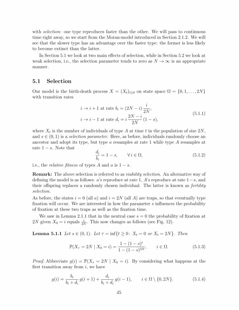
with selection: one type reproduces faster than the other. We will pass to continuoustime right away, so we start from the Moran-model introduced in Section 2.1.2. We willsee that the slower type has an advantage over the faster type: the former is less likelyto become extinct than the latter.
In Section 5.1 we look at two main effects of selection, while in Section 5.2 we look atweak selection, i.e., the selection parameter tends to zero as N →∞ is an appropriatemanner.
5.1 Selection
Our model is the birth-death process X = (Xt)t≥0 on state space Ω = 0, 1, . . . , 2Nwith transition rates
i→ i+ 1 at rate bi = (2N − i) i
2N,
i→ i− 1 at rate di = i2N − i
2N(1− s),
(5.1.1)
where Xt is the number of individuals of type A at time t in the population of size 2N ,and s ∈ (0, 1) is a selection parameter. Here, as before, individuals randomly choose anancestor and adopt its type, but type a resamples at rate 1 while type A resamples atrate 1− s. Note that
dibi
= 1− s, ∀ i ∈ Ω, (5.1.2)
i.e., the relative fitness of types A and a is 1− s.
Remark: The above selection is referred to as viability selection. An alternative way ofdefining the model is as follows: a’s reproduce at rate 1, A’s reproduce at rate 1−s, andtheir offspring replaces a randomly chosen individual. The latter is known as fertilityselection.
As before, the states i = 0 (all a) and i = 2N (all A) are traps, so that eventually typefixation will occur. We are interested in how the parameter s influences the probabilityof fixation at these two traps as well as the fixation time.
We saw in Lemma 2.1.1 that in the neutral case s = 0 the probability of fixation at2N given X0 = i equals i
2N. This now changes as follows (see Fig. 12).
Lemma 5.1.1 Let s ∈ (0, 1). Let τ = inft ≥ 0: Xt = 0 or Xt = 2N. Then
P(Xτ = 2N | X0 = i) =1− (1− s)i
1− (1− s)2N, i ∈ Ω. (5.1.3)
Proof. Abbreviate g(i) = P(Xτ = 2N | X0 = i). By considering what happens at thefirst transition away from i, we have
g(i) =bi
bi + dig(i+ 1) +
dibi + di
g(i− 1), i ∈ Ω \ 0, 2N. (5.1.4)
45

This recursion is to be solved subject to the boundary conditions g(0) = 0 and g(2N) =1. Rearranging the terms in (5.1.4), we may write
[g(i+1)−g(i)] =dibi
[g(i)−g(i−1)] = (1−s) [g(i)−g(i−1)], i ∈ Ω\0, 2N. (5.1.5)
Use g(0) = 0, put c = g(1) and iterate (5.1.5), to get
g(i+ 1)− g(i) = c(1− s)i, i ∈ Ω\2N. (5.1.6)
Summing this relation over i = 0, . . . , j − 1, we obtain
g(j) =
j−1∑i=0
c(1− s)i =c
s
[1− (1− s)j
], j ∈ Ω. (5.1.7)
Since g(2N) = 1, we havec
s=[1− (1− s)2N
]−1. (5.1.8)
Combining (5.1.7–5.1.8), we get the claim.
Fig. 12 shows the effect of selection: the slower type A has a selective advantageover the faster type a, resulting in a bias of the survival probability towards the slowertype. Slow reproduction causes type A to be “less prone to wiping itself out”.
0 1
1
Figure 12: Qualitative picture of (5.1.3).
The average fixation time E(τ) is not so easy to compute, unlike what we saw inSection 2.1 for the neutral WF-model (s = 0), where we found that E(τ | H0) = 2NH0
with H0 the genetic variability at time 0. The following lemma identifies the average ofτ conditional on X0 = 1 and Xτ = 2N .
Lemma 5.1.2 Let s ∈ (0, 1). Then
E(τ | X0 = 1, Xτ = 2N) ∼ 2
slogN as N →∞. (5.1.9)
Proof. The proof is given in Durrett [10], Section 6.1. It is based on a somewhat lengthycalculation showing that it takes time
46

(1) ∼ 1s
logN to go from i = 1 to i = 2NlogN
;
(2) ∼ 2 log logN to go from i = 2NlogN
to i = 2N − 2NlogN
;
(3) ∼ 1s
logN to go from i = 2N − 2NlogN
to i = 2N .
Thus, after the start at X0 = 1 the system spends a long time near 0 (mostly a’s), thenrapidly moves accross and spends a long time near 2N (mostly A’s), until it hits 2N(because of the condition Xτ = 2N).
The fast crossing from mostly a’s to mostly A’s is called a selective sweep.
The computations in Section 2.1 show that, in the absence of selection (s = 0),E(τ | X0 = 1, Xτ = 2N) is of order N , which is much larger than the order logN foundin Lemma 5.1.2.
5.2 Weak selection
Interesting behavior occurs when there is weak selection, in particular, when N → ∞and
s = s(N) =σ
4N, σ ∈ (0,∞). (5.2.1)
Think of 12σ as the fitness advantage of A w.r.t. a in the population. (The choice to
divide by 4N rather than 2N is a matter of convention.)
Write X(N)t to exhibit the N -dependence and define, in analogy with (2.2.1),
Y(N)t =
1
2NX
(N)2Nt, t ≥ 0. (5.2.2)
The following result is the analogue of Theorem 2.2.1. We assume that
w − limN→∞
Y(N)
0 = Y0 (5.2.3)
and ask whetherw − lim
N→∞(Y
(N)t )t≥0 = (Yt)t≥0. (5.2.4)
Theorem 5.2.1 The scaling in (5.2.4) subject to (5.2.3) is true, with (Yt)t≥0 the diffu-sion process on [0, 1] given by the stochastic differential equation
dYt = 12σ Yt(1− Yt) dt+
√Yt(1− Yt) dWt. (5.2.5)
Exercise 5.2.2 Give the proof of Theorem 5.2.1 along the same lines as the proof ofTheorem 2.2.1. Use that
bd2Nye − dd2Nye ∼ 2Ny(1− y)[1− (1− s)] = 2Ns y(1− y) = 12σ y(1− y) N →∞.
(5.2.6)
47

The stochastic differential equation in (5.2.5) has two parts: a deterministic part,given by a logistic drift term pushing the system towards all A, and a random part,given by the WF-diffusion term. Like (2.2.4), it has a unique strong solution. A dualprocess exists, but this is more complex than the death process we encountered inTheorem 2.3.1 acting as the dual process for the WF-diffusion (σ = 0). The dualprocess in the presence of selection requires a graphical construction (see Durrett [10],pp. 127–128). We see from (5.2.2–5.2.4) and Theorem 5.2.1 that under weak selectionthe fixation time is again of order N , so that on time scale 2N the fixation time is oforder 1 (just as for the standard WF-model studied in Section 2.2).
Let us next see what happens when we add mutation. Then the states i = 0 andi = 2N are no longer traps and the system has a non-trivial equilibrium Y (N). Weconsider the limit N →∞ with
u = u(N) =q
4N, v = v(N) =
r
4N, s = s(N) =
σ
4N. (5.2.7)
The following result generalizes Theorem 4.1.2.
Theorem 5.2.3 Subject to (5.2.7), the convergence in (4.1.15–4.1.16) is true, with Ythe random variable on [0, 1] with probability density
f(x) = Cq,r,σ xq−1(1− x)r−1 eσx/2, x ∈ [0, 1], (5.2.8)
with Cq,r,σ the normalizing constant.
Proof. The proof for σ = 0 was based on an asymptotic expansion (recall (4.1.21–4.1.24)). The proof for σ > 0 can be done quickly by comparison with the case σ = 0.To that end, let π(i), i ∈ Ω, be the stationary distribution before passing to the limitN →∞. Then
π(i)di = π(i− 1)bi−1, i ∈ Ω \ 0. (5.2.9)
Hence, we have
π(i)
π(0)=
[i∏
j=1
bj−1
dj
]= b0
[i−1∏j=1
bjdj
]1
di, i ∈ Ω \ 0. (5.2.10)
Let b∗i , d∗i be the birth and death rates for the model without selection, given by (2.1.11),
and let π∗(i), i ∈ Ω, be the associated stationary distribution. For this model the samerecursion as in (5.2.9) applies, namely,
π∗(i)d∗i = π∗(i− 1)b∗i−1, i ∈ Ω \ 0, (5.2.11)
and so the analogue of (5.2.10) reads
π∗(i)
π∗(0)=
[i∏
j=1
b∗j−1
d∗j
]= b∗0
[i−1∏j=1
b∗jd∗j
]1
d∗i, i ∈ Ω \ 0. (5.2.12)
48

Combining (5.2.10) and (5.2.12) with the observation that bi = b∗i and di = d∗i (1 − s),we obtain
π(i)
π(0)= (1− s)−i π
∗(i)
π∗(0), i ∈ Ω \ 0. (5.2.13)
Now pick i = d2Nxe with x ∈ (0, 1) and let N →∞. Then, since
(1− s)−i ∼(1− σ
4N
)−2Nx ∼ eσx/2, n→∞, (5.2.14)
it follows that the equilibrium distribution with selection carries an extra factor eσx/2
compared to the equilibrium distribution without selection, explaining the differencebetween (5.2.8) and (4.1.17). The two equilibrium distributions have different normal-izing constants, which are cancelled out because we divide by π(0), respectively, π∗(0)before taking the limit N →∞. Qualitatively the same pictures as in Fig. 11 apply.
Weak selection tilts the equilibrium achieved under weak mutation.
49

Part II
Multi-colony Wright-Fisherpopulations
In Part I (Chapters 2–5) we considered models where a single population evolves underresampling, mutation and selection. In Part II (Chapters 6–7) we move on to includemigration, i.e., we include the effect of spatial motion. This leads to models with a largenumber of interacting populations.
We imagine that each population lives in a colony and that different colonies are orga-nized into a lattice L, which labels the colonies. In what follows we will consider twochoices:
(1) L = Z2, the square lattice (Chapter 6),(2) L = ΩM , the hierarchical lattice of order M ∈ N (Chapter 7).
We allow the individuals to choose their ancestors not only from their own colony,but also from other colonies, according to a prescribed random walk transition kernelp(x, y), x, y ∈ L. This is called migration, because it causes the types to migratefrom one colony to another. Note that the individuals themselves do not migrate: ineach colony the population remains fixed at 2N individuals, just as in the single-colonyWright-Fisher model.
Migration of types rather than individuals is appropriate e.g. forflowers and plants, where pollen or seeds travel by wind and viainsects. It is less appropriate for animals.
50

6 The stepping stone model
In Section 6.1 we introduce the model. In Section 6.2 we derive a formula for theprobability that two individuals, drawn randomly from the population, are identical bydescent. In Sections 6.3–6.4 we analyze this formula in two different parameter regimes.
6.1 Model
In this section we consider interacting Wright-Fisher populations with mutation butwithout selection. The colonies are labelled by the square lattice (see Fig. 13)
L = Z2 (6.1.1)
and are subject to migration with random walk transition kernel (see Appendix A.2.3)
p(x, y) = (1− ν)δx,y + νq(y − x), x, y ∈ Z2, (6.1.2)
where ν ∈ (0, 1] is a parameter and q : Z2 → [0, 1] is a prescribed probability distributionon Z2. W.l.o.g. we may assume that q(0) = 0.
Figure 13: Z2: sites and nearest-neighbor bonds.
The evolution of the system is as follows:
(1) At each unit of time, each individual mutates to a new type with probabilityµ ∈ (0, 1).
(2) At each unit of time, each individual conditional on no mutation chooses a colonyand adopts the type of a randomly chosen individual from that colony. Individualsin colony x choose colony y with probability p(x, y).
(3) Each colony contains 2N individuals. All individuals mutate and migrate inde-pendently (“parallel dynamics”).
The migration under (6.1.2) amounts to individuals choosing their own colony withprobability 1 − ν and a different colony with probability ν. Given that they choose a
51

different colony, the choice is made with a probability that only depends on the distanceto this colony. The parameter ν is the migration probability. Note that the mutation islike in the infinitely many alleles model studied in Section 3.2: each mutation introducesa new type.
In what follows we will focus on the nearest-neighbor model:
q(z) =
14
if ‖z‖ = 1,0 otherwise.
(6.1.3)
Here, ‖·‖ denotes the lattice norm. We will write p = pν to exhibit that p depends on ν.Most of the results to be described below carry over to more general q, provided it hasthe symmetries of Z2 and decays rapidly at infinity. It is also possible to consider latticesin higher dimensions. For ease of exposition we will not pursue such generalizations.
6.2 Lineages
We are interested in the lineage of two individuals randomly drawn from colonies xand y when the system is in equilibrium. When x = y, we assume that two distinctindividuals are drawn from the colony. Due to the presence of mutations, there are notraps and the system has an ergodic equilibrium.
Let (compare with (4.1.11))
ψ(x, y) = probability in equilibrium that two individuals randomlydrawn from colonies x and y are identical by descent.
(6.2.1)
Clearly, for the analysis of the genealogy of the populations this is a key quantity. Wewill compute ψ(x, y) and study its dependence on x and y. By translation invariance,ψ(x, y) is a function of y − x only.
We begin by expressing ψ(x, y) in terms of ψ(0, 0) and the iterates of the transitionkernel pν(x, y).
Lemma 6.2.1 For all x, y ∈ Z2,
ψ(x, y) =1− ψ(0, 0)
2N
∞∑n=1
(1− µ)2np2nν (x, y). (6.2.2)
Proof. Let ψn(x, y) be the probability in the right-hand side of (6.2.1) at time n whenthe system starts from a given initial configuration (say, all types 0). Then we have therecursion relation
ψn+1(x, y) = (1− µ)2∑z∈Z2
p(x, z)p(y, z)
[1
2N+
(1− 1
2N
)ψn(z, z)
]+ (1− µ)2
∑x′,y′∈Z2
x′ 6=y′
p(x, x′)p(y, y′)ψn(x′, y′).(6.2.3)
52

Here, we sum over the two steps x→ x′ and y → y′ in the lineages of the two individualsbetween time n and time n + 1, and we require that no mutation occurs during eitherof these steps, so that the lineages continue from x′ and y′. The first sum deals withthe case x′ = y′ = z: with probability 1
2Nthe same individual is chosen in colony z
and coalescence occurs, while with probability 1 − 12N
different individuals are chosenin colony z and the lineages continue from z. (Note that each step in the random walkcauses a type to move in the opposition direction.)
By ergodicity, we have
limn→∞
ψn(x, y) = ψ(x, y), x, y ∈ Z2. (6.2.4)
Hence (6.2.3) yields
ψ(x, y) = (1−µ)2∑z∈Z2
p(x, z)p(y, z)1− ψ(z, z)
2N+(1−µ)2
∑x′,y′∈Z2
p(x, x′)p(y, y′)ψ(x′, y′).
(6.2.5)The second sum in (6.2.5) is the limit of the second sum in (6.2.3) with the diagonalpart added. The first sum in (6.2.5) is the difference of the limit of the first sum in(6.2.3) and the diagonal part of the second sum in (6.2.5). The first sum in (6.2.5)gives the first summand in (6.2.2), i.e., the term with n = 1, because ψ(z, z) = ψ(0, 0)and
∑z pν(x, z)pν(y, z) =
∑z pν(x, z)pν(z, y) = p2
ν(x, y) (use the symmetry of pν). Thesecond sum in (6.2.5) can be iterated by resubstitution of (6.2.5). This generates allthe higher summands in (6.2.2), i.e., the terms with n ≥ 2.
Exercise 6.2.2 Explain why the infinite series in (6.2.2) converges (so that the iterativeargument in the proof indeed produces the correct formula).
Abbreviate
Gµ,ν(x, y) =∞∑n=1
(1− µ)2np2nν (x, y). (6.2.6)
Theorem 6.2.3 For µ, ν ∈ (0, 1) and x, y ∈ Z2,
ψ(x, y) =Gµ,ν(x, y)
2N +Gµ,ν(0, 0). (6.2.7)
Proof. By picking x = y = 0 in (6.2.2) and solving for ψ(0, 0), we get
ψ(0, 0) =Gµ,ν(0, 0)
2N +Gµ,ν(0, 0). (6.2.8)
Substituting this into (6.2.2), we get the claim.
With Theorem 6.2.3 we have identified the N -dependence of ψ(x, y), and all thatwe need to do is analyze how Gµ,ν(x, y) behaves as a function of y − x and µ, ν. This
53

is a basic calculation involving simple random walk on Z2 with pausing (recall (6.1.2–6.1.3)). It is straightforward to analyze Gµ,ν(x, y) numerically. Let us see what can bedone analytically.
Durrett [10], Section 5.2, provides a Fourier calculation of Gµ,ν(x, y) for the casewhere the lattice L = Z2 is restricted to a finite box of size L ∈ N,
L = [0, L)2 ∩ Z2, (6.2.9)
with periodic boundary conditions (which turns the box into a torus and preserves thetranslation invariance). It turns out that for this choice there are two regimes:
I. 1µ 1
νL2,
II. 1µ 1
νL2.
(6.2.10)
Regime I corresponds to the system not feeling the boundary of the box. Indeed, 1µ
isthe average time required for a mutation to occur in one lineage. Consequently, ν
µis
the variance of the displacement of a lineage before a mutation occurs (the varianceper step is 1 by (6.1.3)). If this ratio is much smaller than L2, then a mutation willoccur before the lineages notice the boundary of the box, and the behavior of ψ(x, y)will be essentially independent of L. Regime II, on the other hand, corresponds tothe situation where the lineages wrap themselves around the torus many times beforea mutation occurs. In that case, the behavior of ψ(x, y) will depend on L and will bemore delicate. In Sections 6.2–6.3 we look at the two regimes in more detail.
6.3 Regime I
Theorem 6.3.1 Write ψ(x, y) = φ(y − x). In Regime I,
φ(z) ≈ 1
4πνN + log `
[K0
(1
`‖z‖)−K0 (‖z‖)
], (6.3.1)
where ` =√ν/2µ, and
K0(u) =
∫ ∞0
(1 + v2)−1/2 cos(vu) dv, u ∈ (0,∞), (6.3.2)
is the modified Bessel function of the second kind of order 0, which satisfies
K0(u) ∼
log(1/u) for u ↓ 0,√π/2u e−u for u ↑ ∞. (6.3.3)
Proof. See Durrett [10], Section 5.2.
The result in Theorem 6.3.1 shows how, on a sufficiently large box, the probabilityfor two individuals to be identical by descent depends on their distance. The answerinvolves all three parameters N,µ, ν, but not L (subject to the constraint L2 ν/µcharacterizing Regime I). The parameter ` is referred to as the characteristic lengthscale.
54

6.4 Regime II
Regime II is harder to come by. Our first intuition is that the system behaves like a“homogeneously mixing population”, because the lineages wrap themselves around thetorus many times before a mutation occurs and therefore sample the full torus. In otherwords, the system behaves like a Wright-Fisher model with a single colony containing2NL2 individuals, so-called panmictic behavior. However, it turns out that this intuitionis not quite correct. In fact, we will see that panmictic behavior only shows up when
µ 1 and Nν logL, (6.4.1)
which requires that N = N(L) and ν = ν(L), i.e., N and ν depend on L.
In Section 6.4.1 we first look at Regime II without mutation. In Section 6.4.2 weadd mutation and compute ψ(x, y) = φ(y − x).
6.4.1 Regime II without mutation
To investigate Regime II, we first consider the case µ = 0. Since mutations occurindependently of resampling and migration, it will be easy to incorporate them later.
Getting the two lineages to the same colony is necessary to achieve coalescence.Afterwards, either coalescence occurs at that colony (when the lineages choose thesame ancestor), or no coalescence occurs (when the lineages choose different ancestors).In the latter case the lineages must proceed further to achieve coalescence. The timeuntil coalescence equals
τ = T0 + TR (6.4.2)
with
T0 = the time until the two lineages meet in the same colony,
TR = the subsequent time lapse until coalescence.(6.4.3)
Moreover,TR = T1 + T2 + · · ·+ Tσ, (6.4.4)
where (Ti)i∈N are i.i.d. copies of the return times of the two lineages (which are inde-pendent of T0), and σ is an independent geometrically distributed random variable withmean 2N . The reason for σ is that upon each collision the two lineages have probabiliy
12N
to coalesce.
We first focus on T0. We write Pπ for the law of the two lineages when they startfrom two randomly chosen locations in the L-torus.
Lemma 6.4.1 For µ = 0 and ν ∈ (0, 1],
w − limL→∞
T0
(L2 logL)/2πν= EXP(1) under Pπ. (6.4.5)
55

Proof. The proof is given in Cox and Durrett [6]. The intuition is that it takes orderL2 logL steps for the two lineages to visit the L-torus well enough so that they havean appreciable probability to meet somewhere. This corresponds to (L2 logL)/ν timeunits, because each lineage steps with probability ν at each time unit. The exponentiallimiting law is typical for “many trials with small success”: the probability for the twolineages to meet in a given time interval is small and therefore they will meet only aftermany trials.
A more refined result is obtained by looking at two lineages that start not randomlybut at fixed colonies, say x and 0. We write Px,0 for their law, and δ0 for the unitmeasure at 0.
Lemma 6.4.2 For µ = 0, ν ∈ (0, 1] and β ∈ [0, 1],
w − limL→∞
T0
(L2 logL)/2πν= (1− β) δ0 + β EXP(1) under Px(L),0 (6.4.6)
for any x(L) such that
limL→∞
log ‖x(L)‖logL
= β. (6.4.7)
Proof. See Durrett [10], Section 5.3.
Roughly speaking, Lemma 6.4.2 says that, for all β ∈ [0, 1], if the lineages start at dis-tance ‖x(L)‖ = Lβ+o(1) from each other, then there is sharp control over the time whenthey first meet. Note that all scales β ∈ [0, 1] are relevant. Lemma 6.4.1 correspondsto β = 1, because if x is drawn from π, then ‖x‖ = L1+o(1) with a probability tendingto 1 as L→∞.
We next focus on the collision times.
Lemma 6.4.3 For µ = 0 and ν ∈ (0, 1],
E0(TR) = 2NL2 (6.4.8)
and
w − limL→∞
TR2NL2
= EXP(1) under Px,0 uniformly in x on the L-torus. (6.4.9)
Proof. We write E0 because the two lineages start from the same site. The claim in(6.4.8) is a well-known mean recurrence time property of Markov chains, for which werefer to standard textbooks. The claim in (6.4.9) is in the same spirit as before: successonly occurs after many trials.
Exercise 6.4.4 Note that E0(TR) = 2NL2 is independent of ν. What is the intuitionbehind this independence?
56

A comparison of Lemmas 6.4.1–6.4.3 shows that within Regime II there are twosubregimes:
II.A. 1ν
logL N : E(T0) E0(TR),II.B. 1
νlogL N : E(T0) E0(TR).
(6.4.10)
In regime II.A, the starting locations of the two individuals do not matter, while inregime II.B they do matter.
Let us summarize the above observations and formulate the scaling behavior in amore general form that also includes an interpolation between Regime II.A and RegimeII.B. (See Cox, Durrett and Zahle [7] and Cox [5].)
Theorem 6.4.5 If
limL→∞
4πNν
logL= α ∈ [0,∞], lim
L→∞
log ‖x(L)‖logL
= β ∈ [0, 1], (6.4.11)
then under Pπ,
α =∞ : w − limL→∞τcL
= EXP(1) with CL = 2NL2,
α ∈ [0,∞) : w − limL→∞τcL
= EXP(1) with CL = (1 + α)L2 logL2πν
,(6.4.12)
while under Px(L),0,
α =∞ : w − limL→∞τcL
= EXP(1) with CL = 2NL2,
α ∈ [0,∞) : w − limL→∞τcL
= (1− γ)δ0 + γEXP(1) with CL = (1 + α)L2 logL2πν
,
(6.4.13)where
γ = γ(α, β) = β + (1− β)α
1 + α. (6.4.14)
Note that the scaling for Pπ is the same as the scaling for Px(L),0 with β = 1 (in whichcase γ = 1).
6.4.2 Regime II with mutation
Having thus obtained the asymptotics of the time to coalescence, we reintroduce mu-tation and return to the probability of the two lineages being equal by descent, definedin (6.2.1). Writing ψ(x, y) = φ(y − x)(= φ(x− y)), we have
φ(x) = E0,x([1− µ]2τ ),
φ =1
L2
∑x∈[0,L)2∩Z2
φ(x) = Eπ([1− µ]2τ ). (6.4.15)
Inserting w − limL→∞ τ/CL = (1 − γ)δ0 + γEXP(1) into (6.4.15), we compute (with Estanding for either Eπ or Ex,0)
E([1− µ]2τ ) =
∫ ∞0
[1− µ]2t P(τ ∈ dt) =
∫ ∞0
[1− µ]2CLs P(τ
CL∈ ds
)∼ (1− γ) + γ
∫ ∞0
e−2CLs log( 11−µ ) e−s ds = 1− γ + γ
1
1 + 2CL log( 11−µ)
,(6.4.16)
57

where ∼ refers to L→∞. For µ ↓ 0 we have log( 11−µ) ∼ µ, and so we arrive at
E([1− µ]2τ ) ∼ (1− γ) + γ1
1 + 2CLµ, (6.4.17)
where ∼ refers to L→∞ and µ ↓ 0.
We can now insert the various choices for CL and γ appearing in (6.4.11–6.4.14), toobtain the asymptotic behavior of h and h(x) in the various cases. For instance, for h(corresponding to γ = 1) we find that if α =∞, then
h ∼ 1
1 + 4Neff µwith Neff = NL2. (6.4.18)
This is the same as the probability for two individuals to be identical by descent in asingle colony Wright-Fisher model with 2Neff individuals (recall the calculation of χ in(4.1.11) in the proof of Lemma 4.1.1). Thus, in this limit where α = ∞, the steppingmodel behaves as if all individuals are thrown into a single colony and ancestors arechosen in a uniform manner from the entire population, which is the panmictic behavioralluded to at the beginning of this section. In this case, apparently the spatial structureof the stepping stone model is irrelevant and it exhibits so-called mean-field behavior,i.e., all individuals influence each other in the same manner. Similarly, if α ∈ (0,∞),then
h ∼ 1
1 + 4Neff µwith Neff = (1 + α)
L2 logL
4πν=
1 + α
αNL2. (6.4.19)
Here, the effective population size 2Neff is the total population 2NL2 times a moderationfactor 1+α
αthat encapsulates the effect of the spatial structure.
Exercise 6.4.6 Note that 1+αα
> 1. Explain why it is plausible that Neff > NL2.
7 Hierarchical models
In this section we make a different choice for the lattice L labelling the colonies, namely,the so-called hierarchical lattice of order M . We will show that in the limit as M →∞ this model displays universal behavior on large space-time scales. This universalbehavior will turn out to be the result of repeated application of a renormalizationtransformation connecting successive hierarchical levels.
Remark: Renormalization is a key tool in statistical physics, an area that aims todescribe the large space-time behavior of interacting particle systems. The idea is thaton large space-time scales an effective law of large numbers is in force, allowing us to de-scribe the macroscopic behavior of such systems in terms of partial differential equationsthat capture the flow of macroscopic quantities like density, momentum and energy. Anexample is the set of hydrodynamic equations describing the flow of macroscopic quan-tities in fluids and gases. The shape of the hydrodynamic equations is the same for all
58

fluids and gases, but they contain certain effective parameters (like compressibility andviscosity) that depend on the fluid or the gas in question. These effective parametersare the “finger prints” of the specific microscopic interactions and dynamics in the sys-tem after the limit to macroscopic space-time scales has been taken. We will see in thissection that a similar behavior occurs for the stepping stone model on the hierarchicallattice.
In Section 7.1 we define the model. In Section 7.2 we introduce the block averageson successive hierarchical space-time scales. In Section 7.3 we show that these blockaverages behave like autonomous diffusions in the limit as M → ∞, with a diffusionfunction that depends on the scale. In Section 7.4 we analyze the renormalization trans-formation that links the diffusion functions on successive scales and analyze its orbit. Itturns out that the WF-diffusion arises as the universal attractor of the renormalizationtransformation, a fact that is emphasized in Section 7.5.
7.1 Hierarchically interacting diffusions
The hierarchical lattice of order M is the set
ΩM =
x = (xk)k∈N : xk ∈ 0, 1, . . . ,M − 1,
∑k∈N
xk <∞
. (7.1.1)
Think of x as the genetic address of colony x:
x1 is the house, x2 is the street, x3 is the town, x4 is the province, x5 is thecountry, etc.
(See Sawyer and Felsenstein [19] for the genetic background of this choice.) The re-striction
∑k∈N xk < ∞ (i.e., all x end with only zeroes) makes ΩM countable. With
componentwise addition modulo M , ΩM becomes a group.
r r r r r r r r r r r r r r r r r r r r r r r r r r rFigure 14: The hierarchical lattice Ω3 (dots) and its hierarchical distance structure (lines).
On ΩM there is a natural distance, called the hierarchical distance:
‖x− y‖ = mink ∈ N0 : xl = yl ∀ l > k. (7.1.2)
This the height of the first common ancestor of x and y in the tree structure given inFig. 14. The hierarchical distance is in fact an ultrametric:
‖x− y‖ ≤ max‖x− z‖, ‖z − y‖ ∀x, y, z ∈ ΩM . (7.1.3)
In particular, all elements in any two disjoint balls around any two sites have the samedistance to each other.
59

Exercise 7.1.1 Expain why the last two statements are true. Explain the link between(7.1.1) and Fig. 14.
We will be interested in the following system of coupled stochastic differential equa-tions :
dYx(t) = c∑y∈ΩM
p(x, y)[Yy(t)−Yx(t)] dt+√g(Yx(t)) dWx(t), x ∈ ΩM , t ≥ 0, (7.1.4)
where
(1) c > 0 is a constant;
(2) p(x, y) is a non-degenerate random walk transition kernel on ΩM ;
(3) g : [0, 1]→ [0,∞) is a non-degenerate diffusion function;
(4) Wxx∈ΩM is an i.i.d. collection of standard Brownian motions.
As initial condition we take
Yx(0) = θ ∈ (0, 1) ∀x ∈ ΩM . (7.1.5)
The system in (7.1.4) models a collection of interacting Wright-Fisher diffusions withmigration rate c, migration kernel p(x, y), and diffusion function g (recall (2.2.24)). It isa continuous space-time version of the stepping stone model studied in Section 3.1, withc and p(x, y) taking over the role of ν and q(y − x) in (6.1.2). There is no mutation,and the diffusion function g is more general than the diffusion function g∗, given byg∗(x) = x(1 − x) encountered for the Wright-Fisher diffusion in Section 2.1.2. Notethat the first term captures the interaction between the colonies, while the second termis autonomous for each colony.
For each x ∈ ΩM , Yx(t) denotes the fraction of individuals of type A in colony x attime t (in the scaling limit given by (2.2.1–2.2.3)). The colonies evolve via resampling,described by the second term in (7.1.4), and interact via migration, described by thefirst term in (7.1.4). In order for the second term to make sense, we need to place somerestrictions on g. In what follows we will assume that:
(i) g(0) = g(1) = 0;(ii) g(u) > 0 ∀u ∈ (0, 1);(iii) g is Lipschitz on [0, 1].
(7.1.6)
Under these restrictions, (7.1.4) has a unique strong solution, i.e., Yx(t) : x ∈ ΩM ismeasurable w.r.t. the sigma-algebra generated by Wx(s) : x ∈ ΩM , 0 ≤ s ≤ t for allt ≥ 0. The class of functions satisfying (7.1.6) will be denoted by H.
In what follows we will make a special choice for the migration kernel (just as wedid in (6.1.3) for the stepping stone model on Z2), namely,
p(x, y) =1
NM
∑k≥‖x−y‖
1
M2k−1, (7.1.7)
60

where NM is the normalizing constant. This choice, which will turn out to be par-ticularly well adapted to the hierarchical structure of ΩM , amounts to a migrationmechanism in which an individual, for each k ∈ N, with a probability proportionalto 1/Mk−1 chooses “space horizon” k, and randomly chooses a colony from the k-block around its own colony. An easy computation, taking into account (7.1.3), givesNM = M2/(M2 − 1). This constant can be absorbed into the migration rate c.
Exercise 7.1.2 Show that NM = M2/(M2 − 1).
Remark: For the choice in (7.1.7) the random walk on ΩM with transition kernel(7.1.7) is critically recurrent, i.e., recurrent but only just. This is similar to the nearest-neighbor random walk on Z2 treated in Section 5, and allows for a rich behavior as willbe shown in the sequel.
7.2 Hierarchy of space-time scales
We will look at the system along an increasing sequence of space-time scales. To thatend, we define
Y [k]x (t) =
1
Mk
∑y∈ΩM‖y−x‖≤k
Yy(Mkt), x ∈ ΩM , k ∈ N. (7.2.1)
This is the average of the components taken over a block of radius k centered at x,with time speeded up proportional to the volume of the block. Note that Mk = |y ∈ΩM : ‖y − x‖ ≤ k| for all x ∈ ΩM . We will refer to Y
[k]x (·) as the block average around
x on space-time scale k (see Fig. 15).
Figure 15: Picture of a k-block around the site η ∈ Ω3 for k = 1, 2, 3. The site ξ ∈ Ω3 fallsin the k-block for k ≥ 2, but not for k = 1.
The block averages themselves satisfy a system of stochastic differential equations:
dY [k]x (t) = c
∑l∈N
1
M l−1
[Y [k+l]x (M−lt)− Y [k]
x (t)]dt
+
√√√√ 1
Mk
∑y∈ΩM :
‖y−x‖≤k
g(Yy(Mkt)) dW [k]x (t), x ∈ ΩM , t ≥ 0, k ∈ N,
(7.2.2)
61

where W [k]x x∈Ω are i.i.d. standard Brownian motions for every k ∈ N. This system
is deduced from (7.1.4) by: (1) summing over the k-block around x and dividing byits volume Mk; (2) speeding up time by Mk; (3) using the ultrametric property of thehierarchical distance together with the special choice of the migration kernel in (7.1.7);
(4) using the scaling properties dWx(Mkt) =dis
√MkdWx(t) and
√aW +
√bW ′ =dis
√a+ bW ′′ to move all the diffusion terms under the square root.
Exercise 7.2.1 Check (7.2.2).
The initial condition in (7.1.5) becomes
Y [k]x (0) = θ ∈ (0, 1) ∀x ∈ ΩM . (7.2.3)
Looking at (7.2.2), we may get discouraged because this system of coupled diffusionsseems even more complicated than (7.1.4). However, in the limit as M → ∞ a majorsimplification sets in, as we will next explain.
7.3 Local mean-field limit
In this section we look at the successive block averages and identify their behavior inthe limit as M →∞.
k = 0: In this case (7.2.2) reads
dY [0]x (t) = c
∑l∈N
1
M l−1
[Y [l]x (M−lt)− Y [0]
x (t)]dt+
√g(Y
[0]x (t)
)dW [0]
x (t). (7.3.1)
As M → ∞, only the term with l = 1 survives. Moreover, w − limM→∞ Y[1]x (M−1t) =
Y[1]x (0) = θ for all t ≥ 0, by (7.2.3). Therefore we obtain that
w − limM→∞
Y [0]x (t) = Z [0](t) (7.3.2)
with Z [0](t) the solution of the stochastic differential equation
dZ(t) = c[θ − Z(t)] dt+√g(Z(t)) dW (t). (7.3.3)
In other words, in the limit as M →∞ the components decouple and each componentperforms an autonomous diffusion with migration rate c, drift towards θ and diffusionfunction g.
k = 1: As M → ∞, again only the term with l = 1 in (7.2.2) survives. Moreover,
w − limM→∞ Y[2]x (M−1t) = Y
[2]x (0) = θ for all t ≥ 0, by (7.2.3). Furthermore, for fixed
t the familyYy(Mt) y∈ΩM :
‖y−x‖≤1
(7.3.4)
62

decouples and each member converges almost instantly to the equilibrium distributionassociated with (7.3.3), with the drift towards θ replaced by a drift towards Y
[1]x (t), the
instantaneous value of the 1-block average. Thus, as M →∞,
w − limM→∞
1
M
∑y∈ΩM :
‖y−x‖≤1
g(Yy(Mt)) = (Fg)(Y [1](t)), (7.3.5)
where
(Fg)(v) =
∫ 1
0
g(u)νc,v,g(du) (7.3.6)
with νc,v,g the equilibrium distribution associated with the diffusion
dZ(t) = c[v − Z(t)] dt+√g(Z(t)) dW (t), (7.3.7)
which is the same as (7.3.3) but with θ replaced by v. Therefore we conclude that
w − limM→∞
Y [1]x (t) = Z [1](t) (7.3.8)
with Z [1](t) the solution of the stochastic differential equation
dZ(t) = c[θ − Z(t)] dt+√
(Fg)(Z(t)) dW (t). (7.3.9)
Note that this is again an autonomous diffusion, but with a different diffusion functionthan in (7.3.3), namely, Fg instead of g. In Section 7.4 we will give an explicit formulafor the map F defined by (7.3.6–7.3.7).
k ≥ 2: By moving up further in the hierarchy we find, iterating the above argument,that
w − limM→∞
Y [k]x (t) = Z [k](t) (7.3.10)
with Z [k](t) the solution of the stochastic differential equation
dZ(t) = c[θ − Z(t)] dt+√
(F kg)(Z(t)) dW (t) (7.3.11)
with diffusion function F kg, the k-th iterate of F applied to g.
Theorem 7.3.1 The above convergence scheme holds for all c > 0, θ ∈ (0, 1) andg ∈ H, the class defined by (7.1.6).
Proof. The proof is beyond the scope of this course. We refer to Dawson and Greven[8].
The limit M → ∞ is referred to as the hierarchical mean-field limit. In this limiteach colony has a large number of neighbors with which it interacts equally strongly.For each k, the k-block feels a drift towards the value of the (k+ 1)-block around it andequilibrates fast w.r.t. the slower motion of that block, reaching what is called a quasi-equilibrum. The diffusion function of the (k + 1)-block is the average of the diffusionfunction of the constituent k-blocks w.r.t. that quasi-equilibrium (see Fig. 16).
63

s s s s s s
s
. . .
1 2 N − 1 N
block average
Figure 16: Given the value of a block average, the N 1 constituent componentsequilibrate on a time scale that is fast w.r.t. the time scale on which the block averagefluctuates. Consequently, the volatility of the block average is the expectation of thevolatility of the constituent components under the conditional quasi-equilibrium.
7.4 Renormalization transformation
We next move on to studying the renormalization transformation F in detail. Tosimplify the calculations somewhat, we henceforth pick c = 1.
Theorem 7.4.1 For every v ∈ (0, 1) and g ∈ H, the stochastic differential equation in(7.3.7) has a unique ergodic equilibrium νv,g given by
νv,g(du) =1
Nv,g
µv,g(u) du, u ∈ [0, 1], (7.4.1)
where
µv,g(u) =1
g(u)exp
[−∫ v
u
w − vg(w)
dw
], µv,g(0) = µv,g(1) = 0, (7.4.2)
and Nv,g is the normalizing constant.
Proof. The equilibrium νv,g is defined by the requirement that∫ 1
0
(Lv,gf)(u)νv,g(du) = 0 ∀ f ∈ D(Lv,g), (7.4.3)
with
Lv,g = (v − u)∂
∂u+ g(u)
∂2
∂u2(7.4.4)
the generator of the diffusion in (7.3.7) and D(Lv,g) its domain. The latter domain isdense in the set of continuous functions on [0, 1]. After inserting (7.4.1) into (7.4.3),ignoring the normalizing constant and partially integrating the resulting equation (thefirst term once and the second term twice), we get∫ 1
0
f(u)
[− ∂
∂u(v − u)µv,g(u)+
∂2
∂u2g(u)µv,g(u)
]du = 0 ∀ f ∈ D(Lv,g).
(7.4.5)
64

The boundary terms that arise from the partial integration vanish because νv,g puts nomass at 0 and 1. We conclude that the term between square brackets must be zero.Removing one differentiation, we end up with the equation
−(v − u)µv,g(u) +∂
∂ug(u)µv,g(u) = Cv,g, (7.4.6)
where Cv,g is some integration constant. Solving (7.4.6) we find (7.4.2), after we absorbCv,g into the normalizing constant Ng,v.
Exercise 7.4.2 Check the above computations. For the fine details, in particular, issuesof integrability near the boundaries of [0, 1], see Baillon et al. [1].
In view of Theorem 7.4.1, F takes on the form
(Fg)(v) =
∫ 1
0g(u)µv,g(u)du∫ 1
0µv,g(u)du
, v ∈ (0, 1). (7.4.7)
It can further be shown that, for all g ∈ H,
w − limv↓0
νv,g = δ0, w − limv↑1
νv,g = δ1, (7.4.8)
so that(Fg)(0) = g(0) = 0, (Fg)(1) = g(1) = 0. (7.4.9)
Note that F in (7.4.7) is a non-linear integral transform acting on the class H. Nowthat we have an explicit form for F , we can study its iterations.
Theorem 7.4.3 FH ⊂ H.
Proof. We must show that if g ∈ H, then also Fg ∈ H. It is clear from (7.4.9) that Fgsatisfies condition (i) in (7.1.6). From (7.4.1–7.4.2) we see that, for all v ∈ (0, 1), νv,gputs mass everywhere in (0, 1). Therefore Fg satisfies condition (ii) in (7.1.6). Finally,it can be shown (see Baillon et al. [1]) that F lowers the Lipschitz constant, i.e., if
L[g] =def supa,b∈[0,1] :
a6=b
∣∣∣∣g(a)− g(b)
a− b
∣∣∣∣ , (7.4.10)
thenL[Fg] ≤ L[g] ∀ g ∈ H. (7.4.11)
Hence, also condition (iii) in (7.1.6) carries over.
According to Theorem 7.4.3, we can iterate F indefinitely and study its orbit
F kgk∈N0 . (7.4.12)
Our key result is the following universal scaling behavior :
65

Theorem 7.4.4 For all g ∈ H,
limk→∞
kF kg = g∗ uniformly on [0, 1], (7.4.13)
withg∗(u) = u(1− u) (7.4.14)
the Wright-Fisher diffusion function.
Proof. The proof uses the iterates of an associated sequence of Markov kernels. Fixg ∈ H. Let ( denotes composition)
Kg(v, du) = νv,g(du),
K [k]g = KFk−1g KFk−2g · · · Kg, k ∈ N.
(7.4.15)
Our equilibrium νv,g satisfies four relations:
(a)∫ 1
0νv,g(du) = 1,
(b)∫ 1
0uνv,g(du) = v,
(c)∫ 1
0u2νv,g(du) = v2 + (Fg)(v),
(d)∫ 1
0g(u)νv,g(du) = (Fg)(v).
(7.4.16)
Relations (a) and (d) are trivial.
Exercise 7.4.5 Deduce (b) and (c) from (7.4.1).
Iteration of (7.4.16) leads to four relations for the kernel K[k]g :
(a′)∫ 1
0K
[k]g (v, du) = 1,
(b′)∫ 1
0uK
[k]g (v, du) = v,
(c′)∫ 1
0u2K
[k]g (v, du) = v2 + k(F kg)(v),
(d′)∫ 1
0g(u)K
[k]g (v, du) = (F kg)(v).
(7.4.17)
Exercise 7.4.6 Derive these relations.
Now comes a clever trick. Subtract (c′) from (b′), to get∫ 1
0
u(1− u)K [k]g (v, du) = v(1− v)− k(F kg)(v). (7.4.18)
Since the left-hand side is ≥ 0, we see that
kF kg ≤ g∗ uniformly on [0, 1] for all k ∈ N0. (7.4.19)
This is already half of (7.4.13). To get the other half, we proceed as follows. It followsfrom (7.4.19) that limk→∞ F
kg = 0 uniformly on [0, 1]. Hence, (b′) and (d′) give that
w − limk→∞
K [k]g (·) = (1− v)δ0(·) + vδ1(·) ∀ v ∈ (0, 1), (7.4.20)
66

where we use that g vanishes at 0 and 1 only. Inserting the above identity into (7.4.18),we arrive at
limk→∞
[v(1− v)− k(F kg)(v)] = 0 ∀ v ∈ (0, 1). (7.4.21)
Thus we have proved (7.4.13) with pointwise convergence. To get uniform convergence,we use that the family kF kgk∈N0 is uniformly equicontinuous on H, a fact that canbe deduced from the analogue of (7.4.11):
L[Kf ] ≤ L[f ] ∀ f, g ∈ H. (7.4.22)
The proof of (7.4.11) is technical (see Baillon et al. [1]).
7.5 Conclusion
The beauty of Theorem 7.4.4 is that is expresses full universality : no matter whatg ∈ H we pick as the diffusion function for the single components of our system (7.1.4),the diffusion function F kg for the k-blocks (defined by (7.2.1)) with k large are close toa multiple of the Wright-Fisher diffusion function, namely,
F kg ∼ 1
kg∗ as k →∞, (7.5.1)
In other words, Wright-Fisher is a global attractor on large space-time scales.
In retrospect, this universality justifies the fact that we dedicatedan entire course on the Wright-Fisher model!
A Appendix
In this appendix we recall a few basic facts about special probability distributions(binomial, geometric, Poisson, exponential, beta, gamma) and elementary stochasticprocesses (discrete-time and continuous-time Markov chains, Poisson processes, randomwalk, Brownian motion).
A.1 Special probability distributions
I. Discrete:
Binomial distribution BIN(n, p):f(k) =
(nk
)pk(1− p)n−k, k = 0, . . . , n, with n ∈ N, p ∈ (0, 1),
E(X) = np, VAR(X) = np(1− p).
Geometric distribution GEO(p):f(k) = p(1− p)k, k ∈ N0, with p ∈ (0, 1),E(X) = (1− p)/p, VAR(X) = (1− p)/p2.
67

Poisson distribution POISSON(λ):f(k) = e−λλk/k!, k ∈ N0, with λ ∈ (0,∞),E(X) = λ, VAR(X) = λ.
II. Continuous:
Exponential distribution EXP(λ):f(x) = λe−λx, x ∈ [0,∞), with λ ∈ (0,∞),E(X) = 1/λ, VAR(X) = 1/λ2.
Beta distribution BETA(α, β)f(x) = 1
B(α,β)xα−1(1− x)β−1, x ∈ [0, 1], with α, β ∈ (0,∞),
E(X) = α/(α + β), VAR(X) = αβ/(α + β)2(α + β + 1).
Gamma distribution GAMMA(α, β):f(x) = βα
Γ(α)xα−1e−βx, x ∈ [0,∞), with α, β ∈ (0,∞),
E(X) = α/β, VAR(X) = α/β2.
A.2 Elementary stochastic processes
A.2.1 Markov chains
A Markov process is a random process without memory: its future depends on itspresent, not on its past. We focus on time-homogeneous Markov processes, for whichthe transition probabilities or transition rates do not depend on time.
Markov processes in discrete time X = (Xn)n∈N0 on a countable state space Sare characterized by an initial distribution µ = (µi)i∈S and a transition matrix P =(Pij)i,j∈S, with the interpretation
µi = P(X0 = i), Pij = P(Xn+1 = j | Xn = i). (A.2.1)
The distribution at time n is given by the formula
P(Xn = j) = (µP n)j =∑i∈S
µi(Pn)ij. (A.2.2)
Markov processes in continuous time X = (Xt)t≥0 on a countable state space Sare characterized by an initial distribution µ = (µi)i∈S and an infinitesimal generatorL = (Lij)i,j∈S, with the interpretation
µi = P(X0 = i), Lij = limt↓0
1
t
[P(Xt = j | X0 = i)− δij
]. (A.2.3)
Note that Lij ≥ 0 for i 6= j and∑
j∈S Lij = 0: Lij, i 6= j, has the interpretation ofthe rate to jump from i to j, while Lii is minus the rate to jump away from i. Thedistribution at time n is given by the formula
P(Xt = j) = (Ptf)j =∑i∈S
µi(Pt)ij, (A.2.4)
68

where Pt = etL defines a semigroup (Pt)t≥0.
When S is uncountable, sums are replaced by integrals, and some extra care is neededwith the definitions of P and L, Pt, which become operators acting on appropriate setsof test functions f , e.g.
(Lf)(y) =
[d
dtE(f(Xt) | X0 = y)
] ∣∣∣t=0, (Ptf)(y) = E(f(Xt) | X0 = y). (A.2.5)
A.2.2 Poisson process
The Poisson process with rate λ ∈ (0,∞) is the continuous-time Markov process N =(Nt)t≥0 on state space N0, starting at N0 = 0 and making unit increments at randomtimes (Tk)k∈N, with 0 = T0 < T1 < T2 < . . ., such that (Tk+1 − Tk), k ∈ N0, are i.i.d.with distribution EXP(λ). These random times form a random subset of [0,∞), whichis referred to as the Poisson point process with intensity λ. This random subset has theproperty that for any collection of disjoint subsets Ul ⊂ [0,∞), l ∈ I, with I some finiteindex set, the numbers |k ∈ N : Tk ∈ Ul|, l ∈ I, are independent and have marginaldistibutions POISSON(|Ul|), l ∈ I.
A.2.3 Random walk
A random walk on Zd, d ≥ 1, in discrete time is any Markov process X = (Xn)n∈N0 onstate space Zd whose transition matrix is given by
Pij = pj−i, (A.2.6)
where i 7→ pi is some probability distribution on Zd, i.e., the transition probabilities areinvariant under shifts. Due to this property, X has the representation
Xn = X0 + (Y1 + · · ·+ Yn), (A.2.7)
where (Yk)k∈N are i.i.d. with P(Yk = i) = pi.
The same formulas hold in continuous time with Lij = lj−i replacing (A.2.6), wherei 7→ li is any function satisfying li ≥ 0, i 6= 0, and
∑i∈Zd li = 0. The same definitions
apply when Zd is replaced by any set that is a group under the operation +.
A.2.4 Brownian motion
Brownian motion W = (Wt)t≥0 is the continuous-time Markov process on R character-ized by four properties: (1) its increments over disjoint time intervals are independent;(2) its increments over time intervals of length s have distribution N(0, s), the normaldistribution with mean 0 and variance s; (3) it has continuous paths, i.e., t 7→ Wt iscontinuous; (4) W0 = 0.
Brownian motion arises as the space-time scaling limit of simple random walk S =(Sn)n∈N0 on Z, the random walk whose i.i.d. increments are ±1 with probability 1
2each.
69

Namely,
w − limn→∞
(Sdnte√n
)t≥0
= (Wt)t≥0, (A.2.8)
where w − lim denotes weak convergence on path space.
Brownian motion has generator (Lf)(y) = 12f ′′(y), i.e.,
E(f(Wt))− E(f(W0)) = E(∫ t
0
12f ′′(Ws) ds
), (A.2.9)
where f : R→ R is any test function that is twice continuously differentiable.
Diffusion processes are obtained from Brownian motions by changing their localcharacteristics: add a local drift and add a local volatility. Durrett [10], Chapter 7,contains a quick introduction to diffusion processes. The WF-diffusion has generator(Lf)(y) = y(1− y)1
2f ′′(y), i.e.,
E(f(Yt))− E(f(Y0)) = E(∫ t
0
Ys(1− Ys) 12f ′′(Ys) ds
). (A.2.10)
The analogue of (A.2.10) for the Brownian motion with local diffusion function g : R→[0,∞) reads
E(f(Yt))− E(f(Y0)) = E(∫ t
0
g(Ys)12f ′′(Ys) ds
). (A.2.11)
B MRCA-process and F-process
B.1 Look-down construction
To investigate (At)t∈R and (Ft)t∈R, we use Pfaffelhuber and Wakolbinger [18] and the“particle construction” of Donnelly and Kurtz [9], called look-down construction, whichwe will now describe (see Fig. 17).
Identify each element (t, i) of the set R×N with the individual at time t at level i.To describe the births of new individuals in the population, define for all levels i < jthe look-down process Pij = (Pij(t))t∈R as a rate-1 Poisson process on R. At each pointof Pij, level j looks down to level i, which means that the individual at level i producesa copy of itself, which is inserted at level j. For each time t0, when level j looks downto level i, the individuals at levels j, j+ 1, . . . are pushed one level up to make room forthe new individual (t0, j). As time runs forward, the new individual is in turn pushedone level up each time there is a birth at one of the lower levels. To be precise, the newindividual born at level j at time t0 is pushed one level up at all times t1 < t2 < . . .,where tn is a point of Pik for some 1 ≤ i < k < j + n, for all n ∈ N. The evolution overtime of an individual born at level j at time t0 can thus be described by a line of theform
L = ([t0, t1)× j) ∪ ([t1, t2)× j + 1) ∪ ([t2, t3)× j + 2) ∪ · · · ⊂ R× N. (B.1.1)
70

Figure 17: Part of a look-down graph. Biological time is running upwards and level numbersare running to the right. Only (parts of) two lines Lm and Ln are drawn. At time t0 levelj looks down to level i and individual (t0, j) is born. Each time an individual in line Lm ispushed one level up, the individual in line Ln that lives at the same time is pushed one levelup. The backward level process of individual (s0, n) jumps from level j to level i at time t0.
See Fig. 17 for a graphical illustration. For each individual (t, i) ∈ R × N there is aunique line L such that (t, i) ∈ L. An individual at level j is pushed one level up attime t if and only if level k looks down to level i at time t for some 1 ≤ i < k ≤ j.This leaves j(j − 1)/2 possible values for i and k, and therefore pushing rates increasequadratically in j. Hence, t∞ = limn→∞ tn is finite with probability 1. We say that aline L exits at time t∞. Note that each individual in L is “pushed to infinity” as Lexits.
Thus, for each time t0 when level j looks down to level i an individual (t0, j) is born.As time runs forward, the individual is pushed up one level at a time until it reachesinfinity, where the individual dies and its (unique) line L exits at some finite time t∞.The random tree consisting of all lines L ⊂ R×N is known as the look-down graph. Theterm particle construction for the construction just described is justified by identifyingeach individual and its corresponding line with a particle and its trajectory in R× N.
Any line L in the look-down graph backwards in time leads to a coalescence withanother line L′. Indeed, the individual (t0, j) in L that lives at the earliest time of all theindividuals in L lives at a time when level j looks down to level i for some i < j. Sinceindividual (t0, i) has a unique line L′ such that (t0, i) ∈ L′, the lines L and L′ coalescein (t0, i). Thus, the tracing of the evolution of an individual backwards in time doesnot stop at the end (or at the beginning in the forward sense) of its line, but leads toan unambiguous and endless trajectory through different lines in the look-down graph.We will call this trajectory the ancestral lineage of the individual, which we will nowformally construct.
71

First note that the look-down graph always contains the immortal line ω = R×1.Fix s0 ∈ R. For each n ∈ N there is a unique line L = Ln of the form (B.1.1) suchthat (s0, n) ∈ Ln, and a function ΛLn : [t0, t∞) → j, j + 1, . . . , t 7→ i such that(t, i) ∈ Ln. Next, reverse time and let Xn
t = ΛLn(s0 − t), t ∈ [0, s0 − t0]. As timeruns backwards, there comes a time where t > s0 − t0, so that Xn
t is no longer defined.However, since t0 is a point of Pij for some i < j, there exists an m < n such that(t0, i) ∈ Lm and such that Xm
t (in particular) is defined for all t ∈ (s0 − t0, s0 − t′0],where t′0 = inft : ∃j′ ∈ N : (t, j′) ∈ Lm. Now t′0 is a point of Pi′j′ for some i′ < j′.Repeating this argument, we get a sequence n > m > . . . > 1 and a sequence ofintervals In = [0, s0 − t0], Im = (s0 − t0, s0 − t′0], . . . such that ∪iIi = [0,∞). (Indeed,((−∞, s0]× 1) ⊂ L1.) Thus, for any individual (s0, n) ∈ R × N we can define itsbackward level process (Φn(t))t≥0 by letting
Φn(t) : [0,∞)→ N, t 7→ X it if t ∈ Ii. (B.1.2)
The ancestral lineage of an individual (s0, n) equals (t,Φn(t))t≥0. Note that the ancestrallineage of any individual will eventually coalesce with the immortal line, i.e.,
∀n ∈ N ∃ t∗n ∀ t > t∗n : Φn(t) = 1. (B.1.3)
The look-down tree Ts consists of all the ancestral lineages (t,Φn(t))t≥0 of the indi-viduals (s, n), n ∈ N, for some reference time s = s0 (see Fig. 17).
B.2 Look-down construction applied
By the definition of the look-down processes Pij, any two ancestral lineages in Ts coalescewith rate 1. This means that Ts has the same distribution as the coalescent (defined inSection 3.1). The particle construction can therefore be used to describe the evolutionof a population in the WF-diffusion. To that end, let the levels of the individuals at anytime be ordered by persistence, i.e., i < j if and only if the offspring of individual (t, i)outlives the offspring of individual (t, j). Note that with the ordering by persistence,the look-down processes Pij, i < j, suffice to describe each birth in the population inthe WF-diffusion.
B.2.1 Identification of the MRCA-process
In this section we prove Theorem 3.2.2.
Proof. It is enough to show that (At)t∈R coincides with P12. First note that a MRCAin the particle construction must always be at level 1. We will prove that (t, 1) is aMRCA if and only if t is a point of P12.
“⇒”: Observe a MRCA at time t in the coalescent tree and the two individuals thatdirectly descended from the MRCA. (We can identify these two time-t individuals asthe MRCA and its copy.) Then t = As for some s > t and the two oldest families in thetime-s population have each descended from one of the two individuals. This means
72

that the other individuals in the population at time t = As do not have living offspringat time s. The ordering by persistence in the particle construction implies that theseother individuals all have higher levels than the MRCA and its copy. Hence, at timeAs the copy of the MRCA is inserted at level 2. i.e., t is a point of P12.
“⇐”: Let t be a point of P12. Then individual (t, 2) is a copy of individual (t, 1).The ordering by persistence implies that there exists an s > t such that the time-spopulation has descended from the individual (t, 1) and its copy (t, 2), i.e., (t, 1) is theMRCA of the time-s population.
The proof of Theorem 3.2.2 implies that each point t0 of P12 initiates a line LiF ofthe form (B.1.1) where j = 2 and t0 = αi for a certain i ∈ Z. Such a line LiF is calleda fixation line. Let ξi denote the exit time of LiF . Note that at time ξi the offspringof individuals (αi, k), k = 3, 4, . . ., goes extinct. Therefore we have that ξi equals theinfimum of times t at which (αi, 1) is the MRCA of the time-t population, thus it followsthat the exit times of the fixation lines coincide with the points of (Ft)t∈R, i.e., ξi = βifor all i ∈ Z.
Let Ant be the time at which the MRCA of the individuals (t, k), k = 1, . . . , n, lives.Since the MRCA of the first n+1 time-t individuals is a common ancestor of the first ntime-t individuals, we have Ant ≥ An+1
t for all n ∈ N. Define Θn = (Θn(t))t∈R by letting
Θn(t) =
1, if Ant > An+1
t ,0, if Ant = An+1
t .(B.2.1)
and let Nn(t) denote the number of times that Θn−1 jumps from 1 to 0 during the timeinterval [0, t], n > 1. Then Nn = (Nn(t))t∈R is a rate-1 Poisson process (see Donnellyand Kurtz [9], Lemma 3.5). We will use the particle construction to show that thisimplies the following theorem.
B.2.2 Identification of the F-process
In this section we prove Theorem 3.2.3.
Proof. Define βni = inft : Ant = αi. First we prove that the times βni ∞i=−∞ coincidewith the jump times of Nn. Note that βni is the time at which the fixation line LiFreaches level n: βni = inft : (t, n) ∈ LiF. At this time, the MRCA of the first n − 1individuals equals the MRCA of the first n individuals, so that Θn−1(t) jumps from 1to 0 at time t = βni , i.e., Nn jumps at time βni . On the other hand, if Nn jumps at timet, then Θn−1 jumps from 1 to 0 at time t, so t must be the infimum of times at whichthe MRCA of the first n − 1 individuals equals the MRCA of the first n individuals.This implies that a fixation line LiF reaches level n at time t = βni . It follows that thetimes βni ∞i=−∞ are the jump times of the rate-1 Poisson process Nn. Next, since thepoints of (Ft)t∈R are given by βi = limn→∞ β
ni , the theorem follows.
A more intuitive, but less formal argument for the fact that (Ft)t∈R is a rate-1Poisson process is the following. First note that if (Ft)t∈R is a Poisson process, then itsrate equals the rate of (At)t∈R. This is a consequence of Theorem 3.2.1: the expected
73

time between a population and its MRCA is constant. It remains to show that thetime between jumps of the MRCA is exponential. Let Xt and 1 −Xt denote the sizesof the two oldest families in the population at time t. Fix t0 ∈ R. There exists ani ∈ Z such that t0 ∈ [βi, βi+1). The random reproduction in the WF-model impliesthat Xt0 is uniformly distributed on [0, 1]. This also holds conditioned on At0 = αi. Sowe have that Xt is uniformly distributed on [0, 1] for all t ∈ [βi, βi+1). At time βi+1,when the MRCA jumps from αi to αi+1, one of the oldest families dies out and two newoldest families come into existence. These two families are again of random size: fort1 ∈ [βi+1, βi+2) we have that Xt1 (conditioned on At1 = αi+1) is (standard) uniformlydistributed. This implies a memoryless waiting time between jumps of the MRCA, sothat the time between jumps of the MRCA is (standard) exponentially distributed.
To derive Theorem 3.2.1 from the particle construction, let i ∈ Z and consider thefixation line LiF starting at time αi. The infimum Ti of times t for which individual(αi, 1) is a common ancestor of the population at time αi + t equals the time it takesfor LiF to exit. At any level k ∈ N\1 of LiF there are
(k2
)rate-1 Poisson processes to
initiate a push to level k+ 1, so it follows that E(Ti) =∑∞
k=2
(k2
)−1= 2. Now let t ∈ R.
Since Ti = βi − αi, Theorem 3.2.1 holds if and only if E(βi − αi) = E(t − At). Thismay seem counter-intuitive because At = αi if and only if t ∈ [βi, βi+1), but it can beexplained via the so-called waiting-time paradox : a time point is more likely to fall ina long interval than in a short interval between Poisson events.
74

References
[1] J.-B. Baillon, Ph. Clement, A. Greven and F. den Hollander, On the attractingorbit of a non-linear transformation arising from renormalization of hierarchicallyinteracting diffusions, Part I: The compact case, Can. J. Math. 47 (1995) 3–27.
[2] N. Berestycki, Recent progress in coalescent theory, Ens. Mat. 16 (2009) 1–193.
[3] J. Bertoin, Levy Processes, Cambridge Tracts in Mathematics, Vol. 121, CambridgeUniversity Press, Cambridge, 1996.
[4] M.F.J. Carsouw, Wright-Fisher evolution, Bachelor thesis, July 2012, MathematicalInstitute, Leiden University.
[5] J.T. Cox, Intermediate range migration in the two-dimensional stepping stonemodel, Ann. Appl. Prob. 20 (2010) 785–805.
[6] J.T. Cox and R. Durrett, The stepping stone model: new formulas expose old myths,Ann. Appl. Prob. 12 (2002) 1348–1377.
[7] J.T. Cox, R. Durrett and I. Zahle, The stepping stone model. II: Genealogies of theinfinite sites model, Ann. Appl. Prob. 15 (2005) 671–699.
[8] D.A. Dawson and A. Greven, Multiple scale analysis of interacting diffusions,Probab. Theory Relat. Fields 95 (1993) 467–508.
[9] P. Donnelly and T.G. Kurtz, Particle representations for measure-valued populationmodels, Ann. Probab. 27 (1999) 166–205.
[10] R. Durrett, Probability Models for DNA Sequence Evolution (2nd. ed.), Springer,New York, 2008.
[11] S.N. Ethier and T.G. Kurtz, Markov Processes; characterization and convergence,John Wiley & Sons, New York, 1986.
[12] W. Ewens, Mathematical Population Genetics (2nd. ed.), Springer, Berlin, 2005.
[13] R.C. Griffiths and S. Lessard, Ewens sampling formula and related formulae: Com-binatorial proofs, extensions to variable population size and applications to ages ofalleles, Theor. Popul. Biol. 68 (2005) 167–177.
[14] D. Hartl and A.G. Clark, Principles of Populations Genetics, (4th ed.), SinauerAssociates Inc., Sunderland MA, USA, 2007.
[15] J. Hein, M.H. Schierup and C. Wiuf, Gene Genealogies, Variation and Evolution,Oxford University Press, Oxford, 2005.
[16] J.F.C. Kingman, On the genealogy of large polulations, J. Appl. Prob. 19 (1982)27–43.
75

[17] J.F.C. Kingman, The coalescent, Stoch. Proc. Appl. 13 (1982) 235–248.
[18] P. Pfaffelhuber and A. Wakolbinger, The process of most recent common ancestorsin an evolving coalescent, Stoch. Proc. Appl. 116 (2006) 1836–1859.
[19] S. Sawyer and J. Felsenstein, Isolation by distance in a hierarchically clusteredpopulation, J. Appl. Probab. 20 (1983) 1–10.
[20] J. Wakeley, Coalescent Theory, Ben Roberts Publications, Oxford, 2009.
76


