Stochastic processes and Markov chains (part I)Markov ... · Stochastic processes and Markov chains...

Stochastic processes and Markov chains (part I)Markov chains (part I)

Wessel van Wieringenw n van wieringen@vu [email protected]

Department of Epidemiology and Biostatistics, VUmc& Department of Mathematics VU University& Department of Mathematics, VU University

Amsterdam, The Netherlands

Stochastic processes


Example 1Example 1• The intensity of the sun.• Measured every day byMeasured every day by

the KNMI.• Stochastic variable XtStochastic variable Xt

represents the sun’s intensity at day t, 0 ≤ t ≤ T. Hence, Xt assumes values in R+ (positive values only)values only).


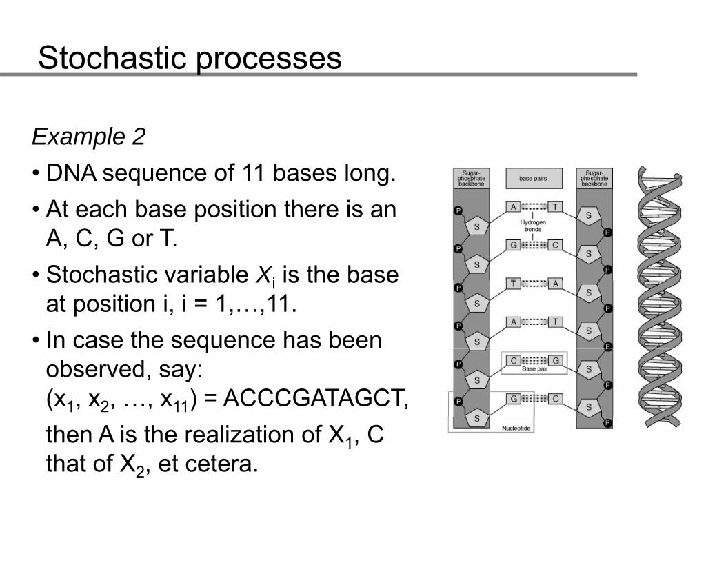
Example 2Example 2• DNA sequence of 11 bases long. • At each base position there is anAt each base position there is an

A, C, G or T.• Stochastic variable Xi is the baseStochastic variable Xi is the base

at position i, i = 1,…,11.• In case the sequence has been q

observed, say:(x1, x2, …, x11) = ACCCGATAGCT,then A is the realization of X1, C that of X2, et cetera.


position … t t+1 t+2 t+3 …base A A T Cbase … A A T C …

A A A A ……

G G G G ……

C C C C ……

T T T T ……

position t

position t+1

position t+2

position t+3


Example 3Example 3• A patient’s heart pulse during surgery.• Measured continuously during interval [0 T]Measured continuously during interval [0, T].• Stochastic variable Xt represents the occurrence of

a heartbeat at time t, 0 ≤ t ≤ T. Hence, Xt assumesa heartbeat at time t, 0 ≤ t ≤ T. Hence, Xt assumes only the values 0 (no heartbeat) and 1 (heartbeat).


Example 4Example 4• Brain activity of a human

under experimentalunder experimental conditions.

• Measured continuouslyMeasured continuously during interval [0, T].

• Stochastic variable XtStochastic variable Xt represents the magnetic field at time t, 0 ≤ t ≤ T. Hence, Xt assumes values on R.

Stochastic processesDifferences between examples

Discrete Continuous

Xt

Discrete Continuous

te

Example 2 Example 1

Dis

cret

DsTi

me

Example 3 Example 4

ntin

uou

Con


The state space S is the collection of all possible valuesThe state space S is the collection of all possible values that the random variables of the stochastic process may assume.

If S = {E1, E2, …, Es} discrete, then Xt is a discrete { 1, 2, , s} , tstochastic variable.→ examples 2 and 3.

If S = [0, ∞) discrete, then Xt is a continuous stochasticIf S [0, ) discrete, then Xt is a continuous stochastic variable.→ examples 1 and 4.p


Stochastic process:• Discrete time: t = 0 1 2 3• Discrete time: t = 0, 1, 2, 3, ….• S = {-3, -2, -1, 0, 1, 2, …..}• P(one step up) = ½ = P(one step down)

67

( p p) ½ ( p )• Absorbing state at -3

345

0123

0-1-2

1 2 3 4 5 6 7 8 9 10 11 12 13 14 15 16 17 18

-3-4

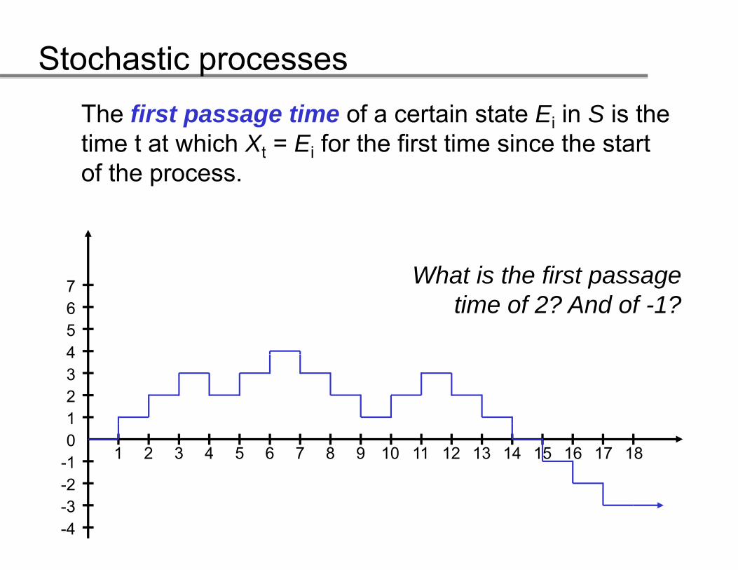
Stochastic processesThe first passage time of a certain state Ei in S is the time t at which Xt = Ei for the first time since the starttime t at which Xt Ei for the first time since the start of the process.

7 What is the first passage

4567 p g

time of 2? And of -1?

1234

0-1-2

1

1 2 3 4 5 6 7 8 9 10 11 12 13 14 15 16 17 18

-3-4

Stochastic processesThe absorbing state is a state Ei for which the following holds: if Xt = Ei than Xt 1 = Ei for all s ≥ tfollowing holds: if Xt Ei than Xt+1 Ei for all s ≥ t. The process will never leave state Ei.

7

4567 The absorbing state is -3.

1234

0-1-2

1

1 2 3 4 5 6 7 8 9 10 11 12 13 14 15 16 17 18

-3-4

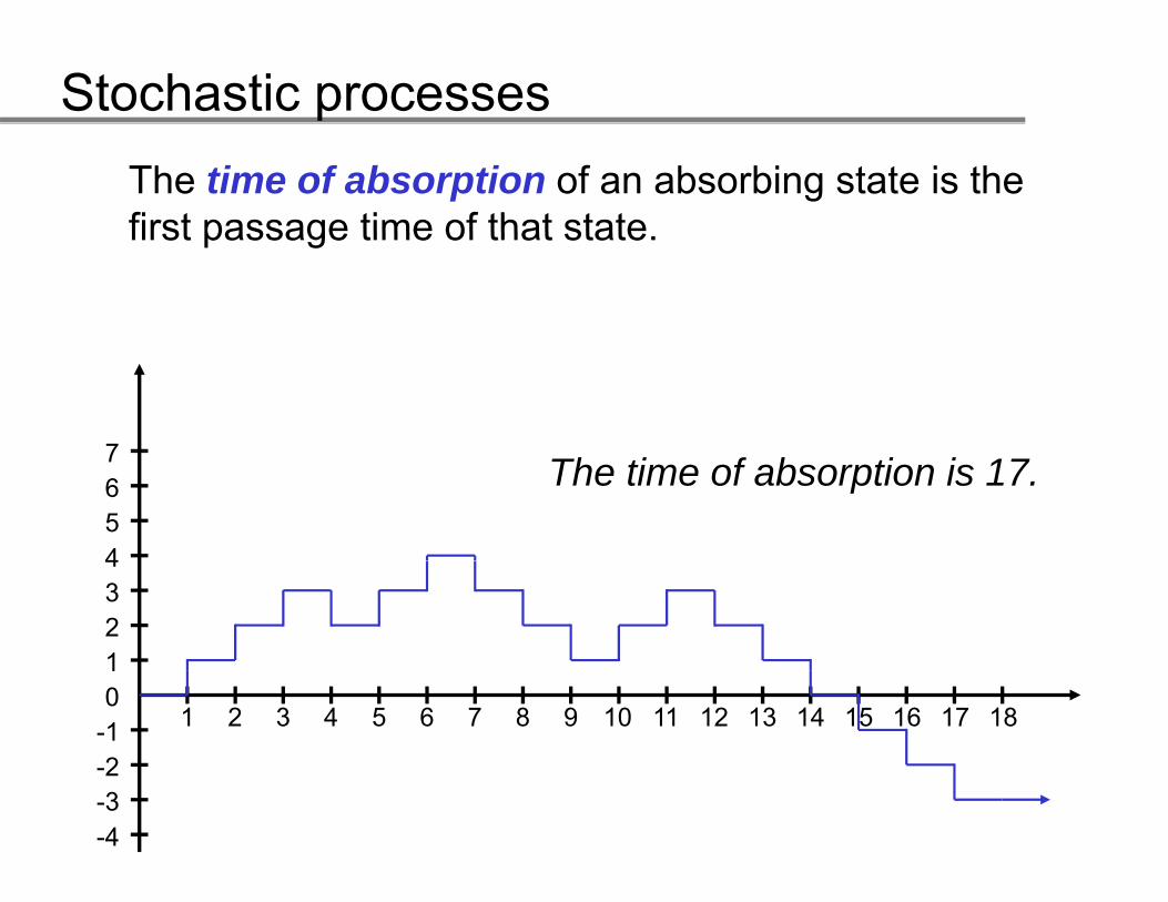
Stochastic processesThe time of absorption of an absorbing state is the first passage time of that statefirst passage time of that state.

7

4567 The time of absorption is 17.

1234

0-1-2

1

1 2 3 4 5 6 7 8 9 10 11 12 13 14 15 16 17 18

-3-4

Stochastic processesThe recurrence time is the first time t at which the process has returned to its initial stateprocess has returned to its initial state.

7

4567 The recurrence time is 14.

1234

0-1-2

1

1 2 3 4 5 6 7 8 9 10 11 12 13 14 15 16 17 18

-3-4


A stochastic process is described by a collection of time points, the state space and the simultaneous distribution of the variables Xt, i.e., the distributions of all X and their dependencyall Xt and their dependency.

There are two important types of processes:• Poisson process: all variables are identically and• Poisson process: all variables are identically and

independently distributed. Examples: queues for counters, call centers, servers, et cetera.counters, call centers, servers, et cetera.

• Markov process: the variables are dependent in a simple manner.p

Markov processes

Markov processes

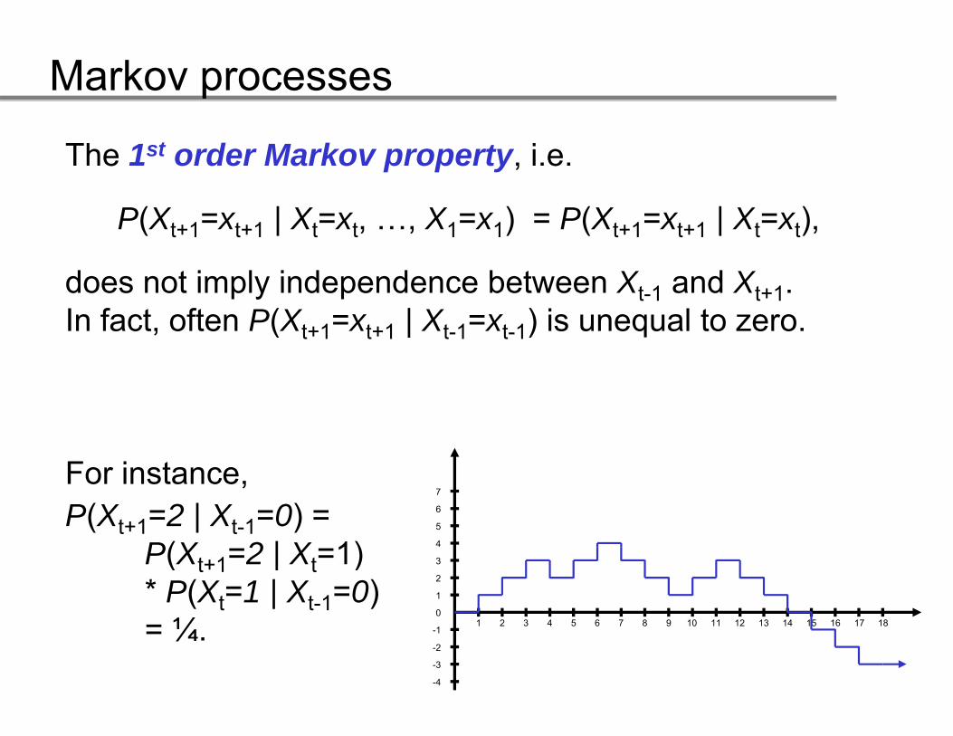
A 1st order Markov process in discrete time is a sto-chastic process {X } for which the following holds:chastic process {Xt}t=1,2, … for which the following holds:

P(Xt+1=xt+1 | Xt=xt, …, X1=x1) = P(Xt+1=xt+1 | Xt=xt).

In other words, only the present determines the future, the past is irrelevant.the past is irrelevant.

From every state with probability 0 5 4

5

6

7

probability 0.5 one step up or down (except 0

-1

1

2

3

1 2 3 4 5 6 7 8 9 10 11 12 13 14 15 16 17 18down (except for state -3).

-2

-3

-4

Markov processes

The 1st order Markov property, i.e.

P(Xt+1=xt+1 | Xt=xt, …, X1=x1) = P(Xt+1=xt+1 | Xt=xt),

does not imply independence between X and Xdoes not imply independence between Xt-1 and Xt+1.In fact, often P(Xt+1=xt+1 | Xt-1=xt-1) is unequal to zero.

For instance, P(Xt+1=2 | Xt-1=0) =

P(X 2 | X 1) 4

5

6

7

P(Xt+1=2 | Xt=1) * P(Xt=1 | Xt-1=0) = ¼

0

-1

1

2

3

1 2 3 4 5 6 7 8 9 10 11 12 13 14 15 16 17 18 ¼.-2

-3

-4

Markov processes

An m-order Markov process in discrete time is a stochastic process {X } for which the following holds:process {Xt}t=1,2, … for which the following holds:

P(Xt+1=xt+1 | Xt=xt, …, X1=x1) = P(Xt+1=xt+1 | Xt=xt,…,Xt-m+1= xt-m+1).

Loosely, the future depends on the most recent past.Loosely, the future depends on the most recent past.

Suppose m=9:

t+19 preceeding bases

… CTTCCTCAAGATGCGTCCAATCCCTCAAAC …

Distribution of the t+1-th base depends on the 9 preceeding ones.

Markov processes

A Markov process is called a Markov chain if the state space is discrete i e is finite or countablespace is discrete, i.e., is finite or countable.

In these lecture series we consider Markov chains inIn these lecture series we consider Markov chains in discrete time.

Recall the DNA example.

Markov processes

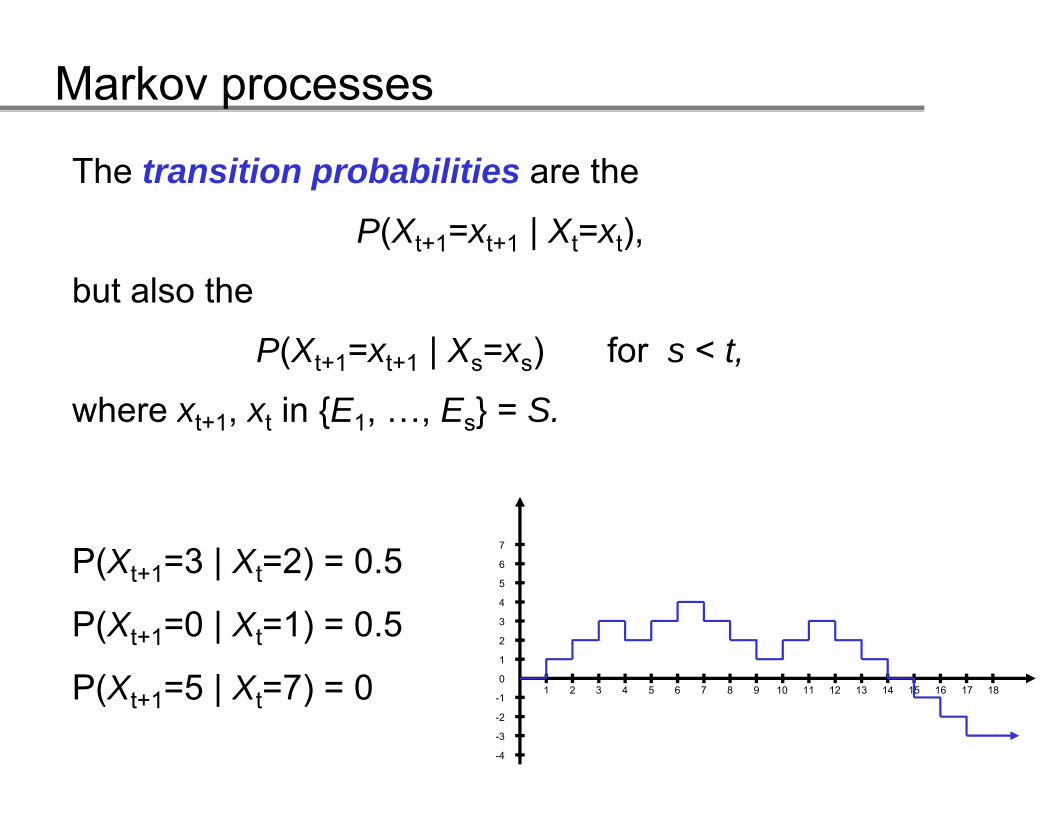
The transition probabilities are the

P(Xt+1=xt+1 | Xt=xt),

but also the

P(Xt+1=xt+1 | Xs=xs) for s < t,

where x x in {E E } = Swhere xt+1, xt in {E1, …, Es} = S.

4

5

6

7

P(Xt+1=3 | Xt=2) = 0.5

0

-1

1

2

3

4

1 2 3 4 5 6 7 8 9 10 11 12 13 14 15 16 17 18

P(Xt+1=0 | Xt=1) = 0.5

P(Xt+1=5 | Xt=7) = 0-2

-3

-4

( t+1 | t )

Markov processes

A Markov process is called time homogeneous if the transition probabilities are independent of t:transition probabilities are independent of t:

P(Xt+1=x1 | Xt=x2) = P(Xs+1=x1 | Xs=x2).

For example:P(X = 1 | X =2) = P(X = 1 | X =2)P(X2=-1 | X1=2) = P(X6=-1 | X5=2)P(X584=5 | X583=4) = P(X213=5 | X212=4)

5

6

7

0

1

1

2

3

4

1 2 3 4 5 6 7 8 9 10 11 12 13 14 15 16 17 18-1

-2

-3

-4

Markov processes

Example of a time inhomogeneous process

h(t) Bathtub curvecurve

t

Infant mortality Random failures

Wearout failures

Markov processes

Consider a DNA sequence of 11 bases. Then, S={a, c, g t} X is the base of position i and {X } is ag, t}, Xi is the base of position i, and {Xi}i=1, …, 11 is a Markov chain if the base of position i only depends on the base of position i-1, and not on those before i-1.the base of position i 1, and not on those before i 1.

If this is plausible, a Markov chain is an acceptable model for base ordering in DNA sequencesmodel for base ordering in DNA sequences.

A C

G TG T

state diagram

Markov processes

In remainder, only time homogeneous Markov processes.

We then denote the transition probabilities of a finite time homogeneous Markov chain in discrete time {Xt}t=1,2,… with S {E E }S={E1, …, Es} as:

P(Xt+1=Ej | Xt=Ei) = pij (does not depend on t).

Putting the pij in a matrix yields the transition matrix:

The rows of this matrix sum to one.

Markov processes

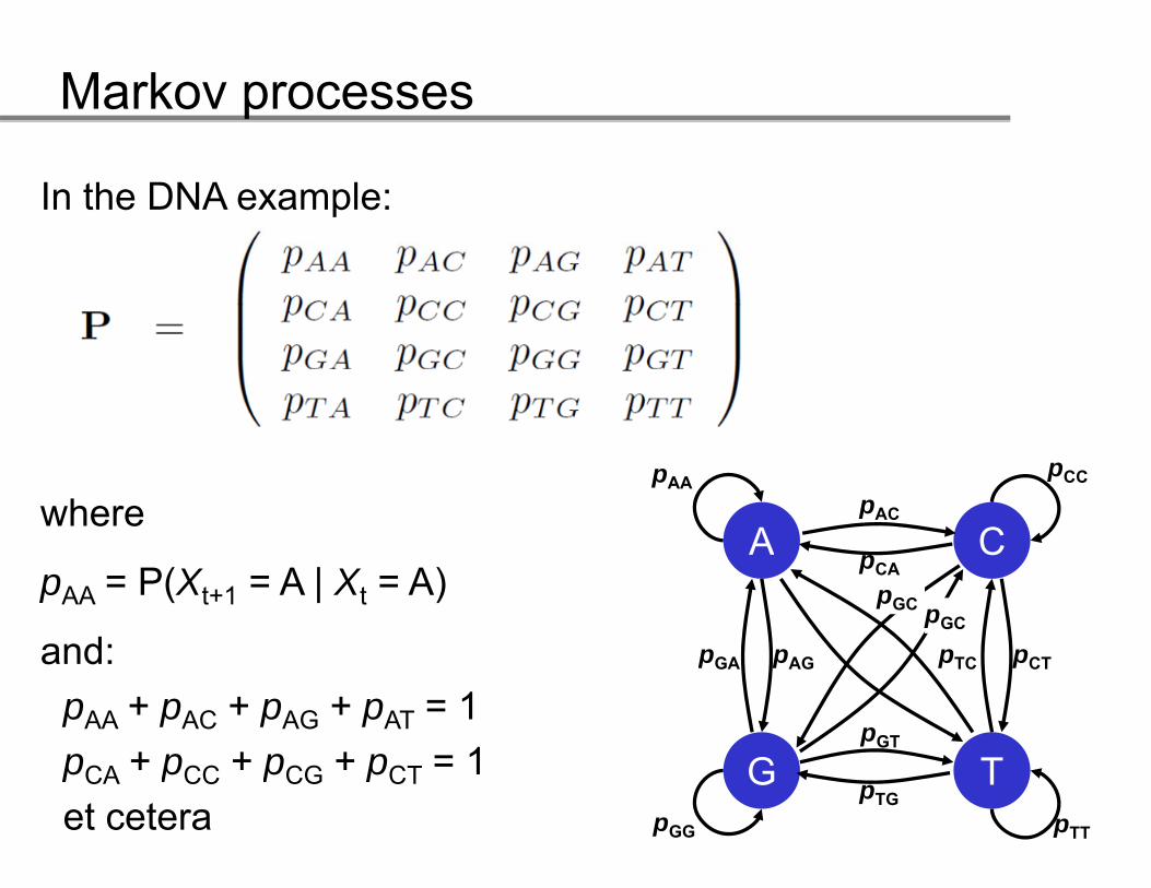
In the DNA example:

A C

pCCpAApACwhere

A CpCA

pTC pCTpGA pAG

pGCpGC

pAA = P(Xt+1 = A | Xt = A)

and:

G TpGT

pTC pCTpGA pAGand:pAA + pAC + pAG + pAT = 1pCA + pCC + pCG + pCT = 1 G T

pTTpGG

pTG

pCA + pCC + pCG + pCT 1et cetera

Markov processes

The initial distribution π = (π1, …,πs)T gives the b bili i f h i i i lprobabilities of the initial state:

πi = P(X1 = Ei) for i = 1, …, s,and π1 + … + πs = 1.

Together the initial distribution π and the transition gmatrix P determine the probability distribution of the process, the Markov chain {Xt}t=1,2, …

Markov processes

We now show how the couple (π P) determines theWe now show how the couple (π, P) determines the probability distribution (transition probabilities) of time steps larger than one. p g

Hereto define for

n = 2 :

lgeneral n :

Markov processes

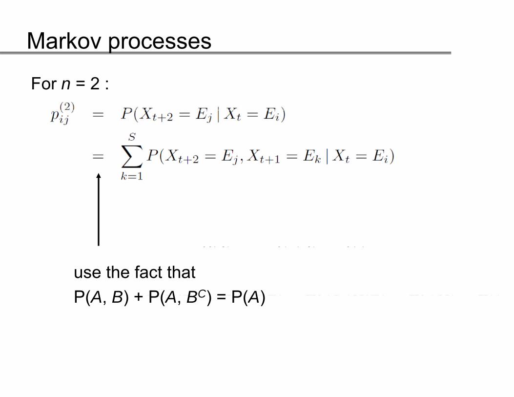
For n = 2 :

just the definition

Markov processes

For n = 2 :

use the fact thatP(A B) + P(A BC) = P(A)P(A, B) + P(A, BC) = P(A)

Markov processes

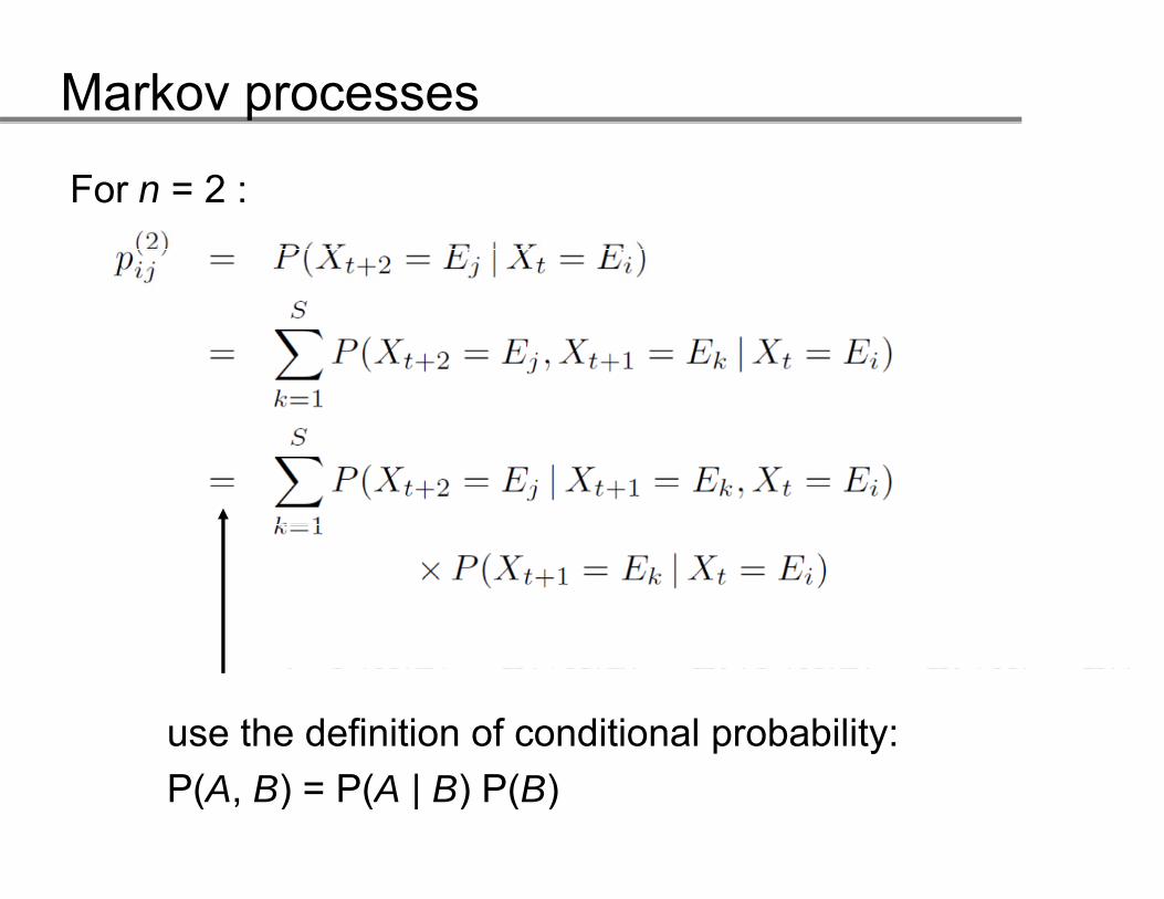
For n = 2 :

use the definition of conditional probability:P(A B) P(A | B) P(B)P(A, B) = P(A | B) P(B)

Markov processes

For n = 2 :

use the Markov property

Markov processes

For n = 2 :

Markov processes

In summary we have shown that:In summary, we have shown that:

In a similar fashion we can show that:In a similar fashion we can show that:

I d th t iti t i f t i thIn words: the transition matrix for n steps is the one-step transition matrix raised to the power n.

Markov processes

The general case:The general case:

is proven by induction to n.

One needs the Kolmogorov-Chapman equations:

for all n, m ≥ 0 and i, j =1,…,S.

Markov processesProof of the Kolmogorov-Chapman equations:

Markov processesInduction proof of

Assume

Then:

Markov processes

A numerical example:

Then:

matrix multiplication (“rows times columns”)matrix multiplication ( rows times columns )

Markov processes

Thus:

0.6490 = P(Xt+2 = I | Xt = I) is composed of two probabilities:

probability of this route plus probability of this route

I I I I I I

II II II II II II

position t

position t+1

position t+2

position t

position t+1

position t+2

Markov processes

In similar fashion we may obtain:

Sum over probs. of all possible paths between 2 states:

I

II

I

II

I

II

I

II

I

II

I

IIII II IIpos. t pos. t+1 pos. t+2

II II IIpos. t+3 pos. t+4 pos. t+5

Similarly:

Markov process

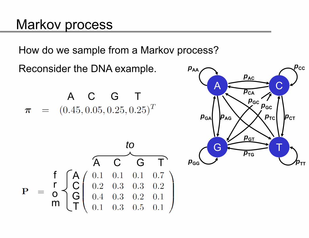
How do we sample from a Markov process?

Reconsider the DNA example.

A C

pCCpAApAC

ppCA

pTC pCTpGA pAG

pGCpGC

A C G T

G TpGT

pTC pCTpGA pAG

to G TpTTpGG

pTG

A C G T

to

Af ACGT

from Tm

Markov process

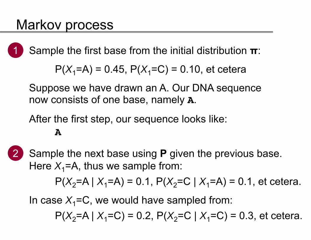
Sample the first base from the initial distribution π:1

P(X1=A) = 0.45, P(X1=C) = 0.10, et cetera

Suppose we have drawn an A. Our DNA sequenceSuppose we have drawn an A. Our DNA sequence now consists of one base, namely A.

After the first step our sequence looks like:After the first step, our sequence looks like:A

Sample the next base using P given the previous base.Here X1=A, thus we sample from:

P(X A | X A) 0 1 P(X C | X A) 0 1 t t

2

P(X2=A | X1=A) = 0.1, P(X2=C | X1=A) = 0.1, et cetera.

In case X1=C, we would have sampled from:P(X2=A | X1=C) = 0.2, P(X2=C | X1=C) = 0.3, et cetera.

Markov process

2 After the second step:AT

3

AT

The last step is iterated ntil the last base3 The last step is iterated until the last base.

After the third step:ATC

9 After nine steps:ATCCGATGCCCG GC

Andrey Markov

Andrey Markov

1856 19221856–1922

Andrey Markov

In the famous first application of Markov chains, AndreyIn the famous first application of Markov chains, Andrey Markov studied the sequence of 20,000 letters in Pushkin’s poem “Eugeny Onegin”, discovering that - the stationary vowel probability is 0.432, - the probability of a vowel following a vowel is 0.128, and

the probability of a vowel following a consonant is 0 663- the probability of a vowel following a consonant is 0.663.

Markov also studied the sequence of 100,000 letters in Aksakov’s novel “The Childhood of Bagrov, the Grandson”.

This was in 1913 long before the computer age!This was in 1913, long before the computer age!

Basharinl et al. (2004)

Parameter estimation

Parameter estimationT A G T T C G G A A G C A C G T G G A T G A G G A A C C C G C C A C C C C A T C C G C C T G G T G T T T G A T A G C T G T A T T C G G G C A T G G C G G C C C A C G C T A T T C G T C T G T A C G C A A G C C T C G T T T T A T C C C C G C C G C C A G A G T A C C G C A G C A C C C G G C G C G A C G G G A C C G C G C C G C G G C C A A C T A G C G C A G C C G C A G A C C G C C A C G T G C G C A G G A C T T C C C A C C C T C A C C C T T C C G C T C A C C C T T A T C G G A G G G C A C T C G C A C G G A T A G T T G G T A G G G G G A C A T C C C A G G G T A G C C G C A C G A T G C G G A T A G G G G T A T T T A T G G C G C C C T C A C C C A G G C G A T C T C G G G C C C G G C T G G G C G C C G G G C G G A C C C A G A T A G A T C G G T G C C C C G G C C C C A A C C G A A G G G T A G G A C T G T C G G A C C T G C G G C G C C C G C G A C G A T A C G A C A G A C A G G A A A G A A A G C A T C C A G G G A C G G C G C G C T T G C T G G A C T G A C C A G C C A C T C C A T G G G G T C C G T A C C C G C C C G G G G G C A C T T T C G C C C C C G C G G A G A G C T G A G A C A A T C G A T G T G C C C A G C C G A G G G G G C C C G C C A G C C C A G G G G A C C G G A C T A A G G G C C A C C G T A G G G T A C A G C A A C C C C G G A C A C T G G C G A C C C C G C A C C A C C C C C A C C C G T A G C T C A G T A C A C G A G G A G A G G A A C C C G C G C G A A G C C C C T G G G C G C T C T T G C T G G T C A G A A A T A C C G T C G T T T A T C C G T G G A C T C G T A C G A C C T G C C A C C C T G G C A G G A C T G A C T G C C G C C A C C C C C C G T C C A C T A C G G A A A G T G A G G G G G C C A A C C G C G T A G G A C A A G A G G G T C T C G C C T C G G G G G G T T G C C G G C C G G G G C A G G T T C A G G A G T T A T T T C C A G G C C C C A C G G A C T G T T T T T C C G T C C C A G A T G G G A T G G A A T T A A C G C A C G C C A T C A C A C C T G C A C G C C G G C C C C C T G G A G A C C G T G C G C A A G A G G G G G C T A C C C A C T T T C T G C G T A T A T A C G T T A G G A C T C G A A G C C C A G G G T A G T G A C G G A C G C G C T C G A T C C C C C G T T C A C C G G G A C C C T G C C G G A T T T A A G G C G C G T G C C G G G C C C G T G C T C A C C C C C G G A C A G C C A G A C A C A T T T C T C C T G C G A G T G G T G C C G C T T A C C G G G T C T G A T A C G G A G T A G A G G C C C C C C G G C T A T A G C C A C A T G C C T A C A T C C T C G C G T C A C A C G G G C T C A G T T C G C C T G G G

How do we estimate the parametersof a Markov chain from the data?

A G T A G A G G C C C C C C G G C T A T A G C C A C A T G C C T A C A T C C T C G C G T C A C A C G G G C T C A G T T C G C C T G G G G A C G G A T G C C C C G A T C G C G T G G G A T A C C C G C G G C T T A C G A A T C A A A C A C G C C G C G G C G T G C G G G C G G G G A G G C C T A G G C T T C G G G A G G G G C A T T G C G C C C T C G A T A C G A C C G G G T C C C C G C C C A C G C T C T T T G G G T G T C G G C G C C G C A C T C C C T G C G T G C C G G T C T C C T T G T G T A A C G G T G A T A C G G G G G T A C C G G T G T G C C A G C A G G C C T C T A A G C T A T A G C C C C T G C C C A C C T T C G T G A C A C C C G G G T T G C C C C C A C G T C C C G G T A G T C A A A G G G C T A C C C A G C G C C G C A T C G A C G T C C C T T G G G T G G C G G T T A A C A G C A G A T C T T T G C C A G A A G T C G C G C A A C A A A G G C A C T C T G C A G C C T G G C C A C C A G G C G G C C C T C T C G A G C G G C C A G C A G G A C C C

Maximum likelihood!A G T C G C G C A A C A A A G G C A C T C T G C A G C C T G G C C A C C A G G C G G C C C T C T C G A G C G G C C A G C A G G A C C C G G G C A C G G C A C T C T A T A G C A C G G T A G C C A C T G C A G T A C C G T A G G A C C A C C C G G T G A C A C A G T G G A G A C C G G G G T T A C A C C A C T C C C C C G A G G T T A G C C A T C C T C G A G A A C G A C T A A G C G C G G G A A C G A G G C G A G C A G C C A A T A C G T G C G A A G A A C G T C T G C G G A G C G C C A T A C A C G A T A A C T A C G G T T T A T A G G T A C G T C G C A T G G A G G T T C G C G G C T G T A A A A C C C A C A C A T A C T C G G T C C C A C A C G G G T G T A A G C A C T C G T C A G T C C G C A G C C T C G T C T C G C C G A G G A T C A C G A G T C G G T C G C C C T C A A A G G A G C T T C A A G T T G G A C C C T G A C C G G G G A C T T G A G A A G T A A G C A C G C C C G A C G A A G C G G G G C C A G C A C C G G T A A A C C T G C G A C A A G T C C T T T A C C G C T A G G G T A C T G C G T G T C A A C C A G T C A C G A G T G C C C C A C C C T G G C G A C C C G G C G A G G A C C G C C C C C T T C C G G G A A G G T C A G A C C T G T G A G C A G A G A G C C A G G A T G C C A C T A A C G C T C A C C G T A C C T T C C G C C T G A C T C G C C G G T C C G C G C G C G A G C A A C C C C T A A C C A C C A A C C G G C G G A G G A C C C A G C A G A A T A T G G C G A A C C G G C C C C C G C G A C T G C G C G A T C G G C A G A C T C C T G T G C G G G G A G C A T A C A G G C T C T C C T C G G A G C G T G G C T C A G T G C C G C G T G G G C C G C T T T C T C C A G C C C C T A C A C G C C C A C T A C T C G A A C G T T T T T G T G G G C C T G A C T T G C C G C G T A C C C G C G C C T T T C G C C C T G A C G A C C C G C G T T A C C T A T G A G G G A T C A T G T G G G G T G G G G C C C C G G G T C C A C G C T A T C G A C G T A T G G T T G C T G C G T C A A C T C A C G C T C G A T G T A C A C G C C G T C C T C G T A A C A G C G A C C A C G C T C C C G A A G C T G G A T A A A C G A C T T C A G C A A T A A G G G A C G G T C A G G G G G G A G G A C G T A C G T A C T G G G C A G G C A G G C G G C T G G C A C C C T G A G G C A A A T G C G G A C G C G A A C C A T C C A A G A C G G G C G A C A A A A C G A C C G G A A G A G C G A G G A G A C G T A G C A C C G T T T C C G C G G C T T C C G A A C G G A G C T A A C A G A G A C C C G C C G G A T C T C G T T G G T A C C G A G C C G C C G T A T A C A T C A C A C C T G C A C G G C C A G T G C C T G C C T T A G T T C G G G C G C T A G C C C G T C G T C C C T A T T T A A C T G C G C G A G T G G C G A G C T C G G C


Using the definition of conditional probability, the Using the definition of conditional probability, the likelihood can be decomposed as follows:

where x1, …, xT in S = {E1, …, ES}.


Using the Markov property, we obtain:Using the Markov property, we obtain:


Furthermore, e.g.:Furthermore, e.g.:

where only one transition probability at the time enters the likelihood due to the indicator functionlikelihood, due to the indicator function.


The likelihood then becomes:The likelihood then becomes:

where, e.g.,


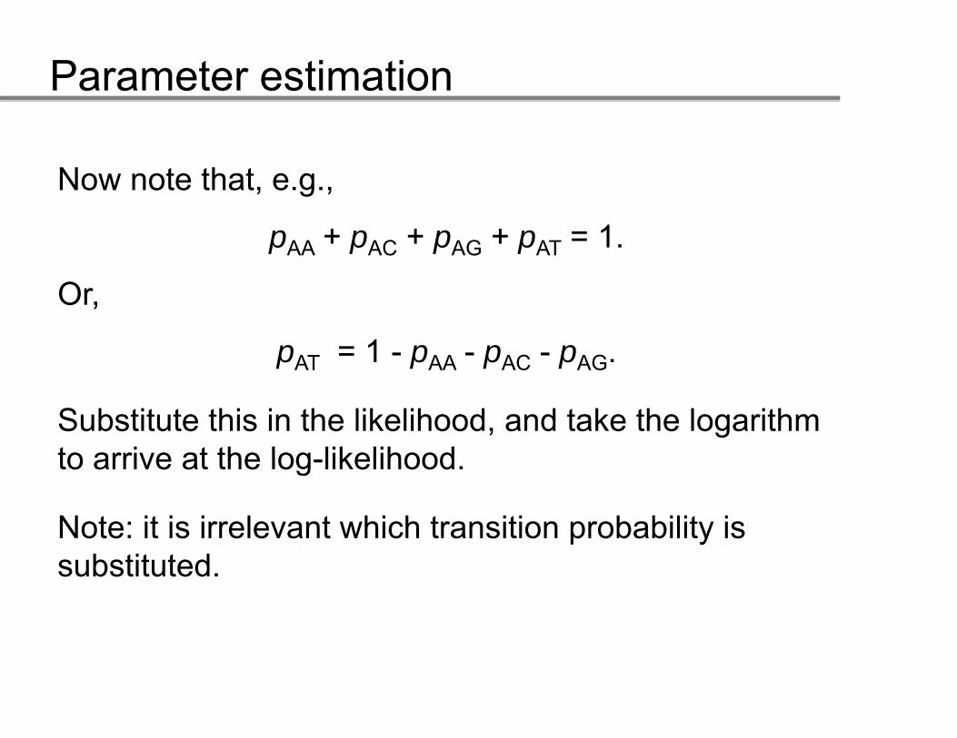
Now note that, e.g., Now note that, e.g.,

pAA + pAC + pAG + pAT = 1.

Or,

pAT = 1 - pAA - pAC - pAG.AT AA AC AG

Substitute this in the likelihood, and take the logarithm to arrive at the log likelihoodto arrive at the log-likelihood.

Note: it is irrelevant which transition probability is substituted.


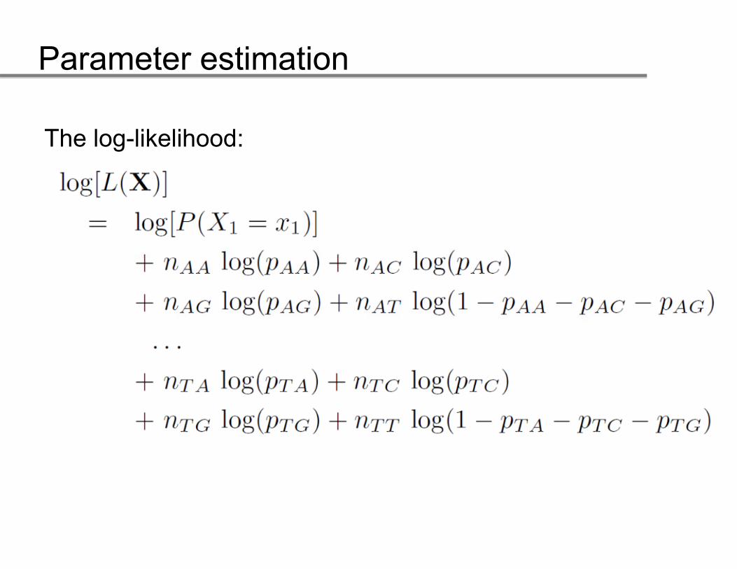
The log-likelihood:The log likelihood:


Differentiation the log-likelihood yields, e.g.:Differentiation the log likelihood yields, e.g.:

Equate the derivatives to zero. This yields four systems of equations to solve e g :equations to solve, e.g.:

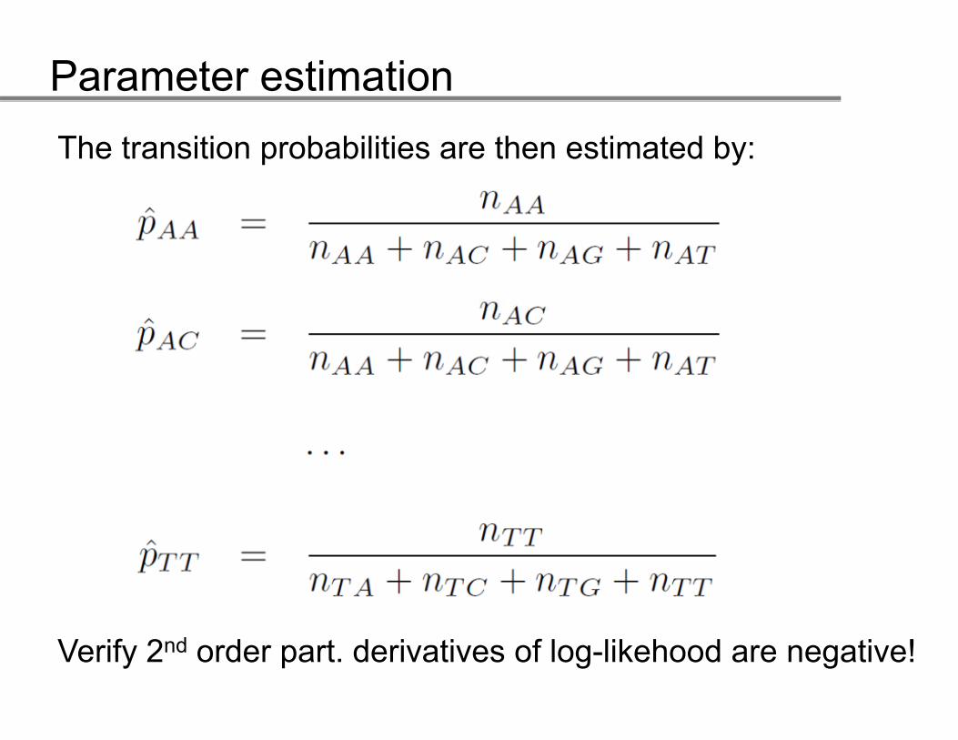
Parameter estimationThe transition probabilities are then estimated by:

V if 2 d d t d i ti f l lik h d ti !Verify 2nd order part. derivatives of log-likehood are negative!


If one may assume the observed data is a realization of a If one may assume the observed data is a realization of a stationary Markov chain, the initial distribution is estimated by the stationary distribution.

If only one realization of a stationary Markov chain is y yavailable and stationarity cannot be assumed, the initial distribution is estimated by:


Thus, for the following sequence: ATCGATCGCA,, g q ,tabulation yields

The maximum likelihood estimates thus become:


In R:> DNAseq <- c("A", "T", "C", "G", "A",

"T", "C", "G", "C" "A")> table(DNAseq)DNAseqA C G TA C G T 3 3 2 2 > table(DNAseq[1:9], DNAseq[2:10])> table(DNAseq[1:9], DNAseq[2:10])

A C G TA 0 0 0 2C 1 0 2 0G 1 1 0 0T 0 2 0 0T 0 2 0 0

Testing the order ofTesting the order of the Markov chainthe Markov chain

Testing the order of a Markov chain

Often the order of the Markov chain is unknown and d b d i d f h d Thi i d ineeds to be determined from the data. This is done using

a Chi-square test for independence.

Consider a DNA-sequence. To assess the order, one first tests whether the sequence consists of independenttests whether the sequence consists of independent letters. Hereto count the nucleotides, di-nucleotides and tri-nucleotides in the sequence:q


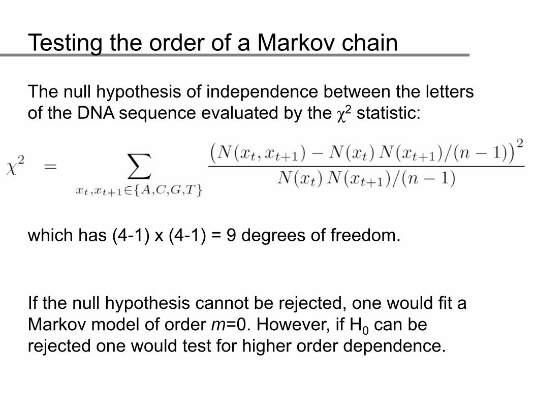
The null hypothesis of independence between the letters f th DNA l t d b th 2 t ti tiof the DNA sequence evaluated by the χ2 statistic:

which has (4-1) x (4-1) = 9 degrees of freedom.

If the null hypothesis cannot be rejected one would fit aIf the null hypothesis cannot be rejected, one would fit a Markov model of order m=0. However, if H0 can be rejected one would test for higher order dependence.


To test for 1st order dependence, consider how often a di-nucleotide e g CT is followed by e g Tnucleotide, e.g., CT, is followed by, e.g., T.

The 1st order dependence hypothesis is evaluated by:The 1st order dependence hypothesis is evaluated by:

wherewhere

This is χ2 distributed with (16 1) x (4 1) = 45 d o fThis is χ2 distributed with (16-1) x (4-1) = 45 d.o.f..


A 1st order Markov chain provides a reasonable description of the sequence of the hlyE gene of the E coli bacteriasequence of the hlyE gene of the E.coli bacteria.

Independence test:Chi-sq stat: 22.45717, p-value: 0.00754q , p

1st order dependence test: Chi-sq stat: 55.27470, p-value: 0.14025

The sequence of the prrA gene of the E.coli bacteria requires a higher q p g q gorder Markov chain model.

Independence test:hi 33 51356 l 1 266532 04Chi-sq stat: 33.51356, p-value: 1.266532e-04

1st order dependence test: Chi-sq stat: 114 56290 p-value: 5 506452e-08Chi-sq stat: 114.56290, p-value: 5.506452e-08

Testing the order of a Markov chainIn R (the independence case, assuming the DNAseq-object isa character-object containing the sequence): j g q )> # calculate nucleotide and dimer frequencies> nuclFreq <- matrix(table(DNAseq), ncol=1)> dimerFreq <- table(DNAseq[1:(length(DNAseq)-1)],

DNAseq[2:length(DNAseq)])

> # calculate expected dimer frequencies> dimerExp <- nuclFreq %*% t(nuclFreq)/(length(DNAseq)-1)

> # calculate test statistic and p-value> teststat <- sum((dimerFreq - dimerExp)^2 / dimerExp)> pval <- exp(pchisq(teststat 9 lower tail=FALSE> pval < exp(pchisq(teststat, 9, lower.tail=FALSE,

log.p=TRUE))

E i dif th d b f th 1st d t tExercise: modify the code above for the 1st order test.

Application: ppsequence

di i i tidiscrimination

Application: sequence discrimination

We have fitted 1st order Markov chain models to a We have fitted 1 order Markov chain models to a representative coding and noncoding sequence of the E.coli bacteria.

Pcoding PnoncodingA C G T

A 0.321 0.257 0.211 0.211C 0.319 0.207 0.266 0.208

A C G TA 0.320 0.278 0.231 0.172C 0.295 0.205 0.286 0.214

G 0.259 0.284 0.237 0.219T 0.223 0.243 0.309 0.225

G 0.241 0.261 0.233 0.265T 0.283 0.238 0.256 0.223

These models can used to discriminate between coding and noncoding sequencescoding and noncoding sequences.


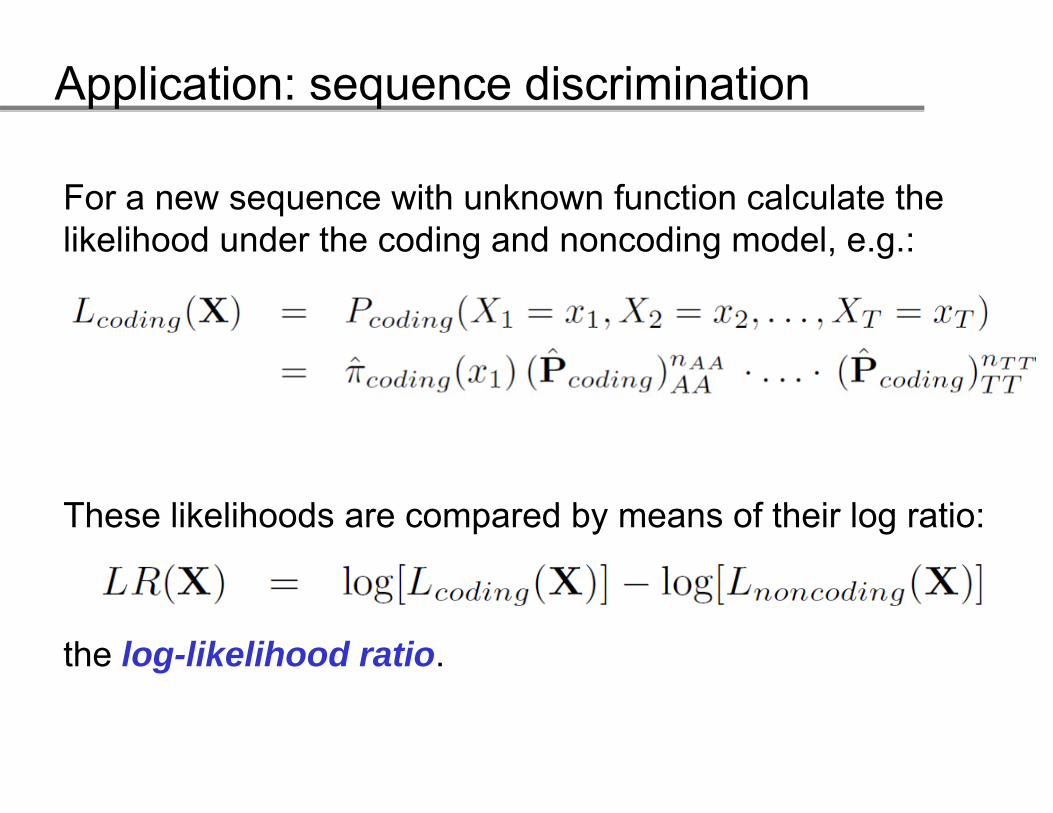
For a new sequence with unknown function calculate the For a new sequence with unknown function calculate the likelihood under the coding and noncoding model, e.g.:

Th lik lih d d b f th i l tiThese likelihoods are compared by means of their log ratio:

the log-likelihood ratio.


If the log likelihood LR(X) of a new sequence exceeds a If the log likelihood LR(X) of a new sequence exceeds a certain threshold, the sequence is classified as coding and non-coding otherwise.

Back to E.coliTo illustrate the potential of the discrimination approach, p pp ,we calculate the log likelihood ratio for large set of known coding and noncoding sequences. The distribution of the t t f LR(X)’ dtwo sets of LR(X)’s are compared.


di di

cy

noncoding sequences

coding sequences

frequ

enc

f

log likelihood ratio

Application: sequence discriminationflip mirror

violinplotviolinplot

noncoding coding


Conclusion E.coli exampleConclusion E.coli exampleComparison of the distributions indicate that one could discriminate reasonably between coding and noncoding y g gsequences on the basis of simple 1st order Markov.

Improvements:- Higher order Markov model.- Incorporate more structure information of the DNA.

References &References & further readingfurther reading

References and further reading

Basharin, G.P., Langville, A.N., Naumov, V.A (2004), “The life and work of A.A. Markov”, Linear Algebra and its Applications 386 3 26and its Applications, 386, 3-26.

Ewens, W.J, Grant, G (2006), Statistical Methods for Bioinformatics Springer New YorkBioinformatics, Springer, New York.

Reinert, G., Schbath, S., Waterman, M.S. (2000), “Probabilistic and statistical properties of words: anProbabilistic and statistical properties of words: an overview”, Journal of Computational Biology, 7, 1-46.

This material is provided under the Creative CommonsThis material is provided under the Creative Commons Attribution/Share-Alike/Non-Commercial License.

See http://www.creativecommons.org for details.

Date post:	09-Apr-2018
Category:	Documents
Upload:	nguyenthuy
View:	260 times
Download:	6 times

Stochastic processes and Markov chains (part I)Markov ... · Stochastic processes and Markov chains...

Documents