J. Virtamo 38.3143 Queueing Theory / Stochastic processes 1

STOCHASTIC PROCESSES

Basic notions

Often the systems we consider evolve in time and we are interested in their dynamic behaviour,

usually involving some randomness.

• the length of a queue

• the temperature outside

• the number of students passing the course S-38.143 each year

• the number of data packets in a network

A stochastic process Xt (or X(t)) is a family of random variables indexed by a parameter t

(usually the time).

Formally, a stochastic process is a mapping from the sample space S to functions of t.

With each element e of S is associated a function Xt(e).

• For a given value of e, Xt(e) is a function of time(“a lottery ticket e with a plot of a func-

tion is drawn from a urn”)

• For a given value of t, Xt(e) is a random variable

• For a given value of e and t, Xt(e) is a (fixed) number

The function Xt(e) associated with a given value e is called the realization of the stochastic

process (also trajectory or sample path).

J. Virtamo 38.3143 Queueing Theory / Stochastic processes 2

State space: the set of possible values of Xt

Parameter space: the set of values of t

Stochastic processes can be classified according to whether these spaces are discrete or con-

tinuous:

State space

Parameter space Discrete Continuous

Discrete ∗ ∗∗

Continuous ∗ ∗ ∗ ∗ ∗ ∗∗

According to the type of the parameter space one speaks about discrete time or continuous time

stochastic processes.

Discrete time stochastic processes are also called random sequences.

J. Virtamo 38.3143 Queueing Theory / Stochastic processes 3

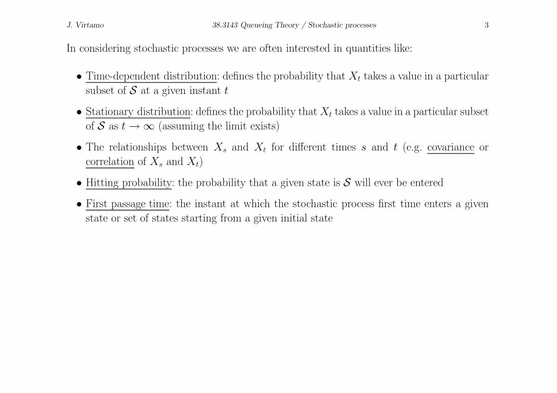
In considering stochastic processes we are often interested in quantities like:

• Time-dependent distribution: defines the probability that Xt takes a value in a particular

subset of S at a given instant t

• Stationary distribution: defines the probability that Xt takes a value in a particular subset

of S as t → ∞ (assuming the limit exists)

• The relationships between Xs and Xt for different times s and t (e.g. covariance or

correlation of Xs and Xt)

• Hitting probability: the probability that a given state is S will ever be entered

• First passage time: the instant at which the stochastic process first time enters a given

state or set of states starting from a given initial state

J. Virtamo 38.3143 Queueing Theory / Stochastic processes 4

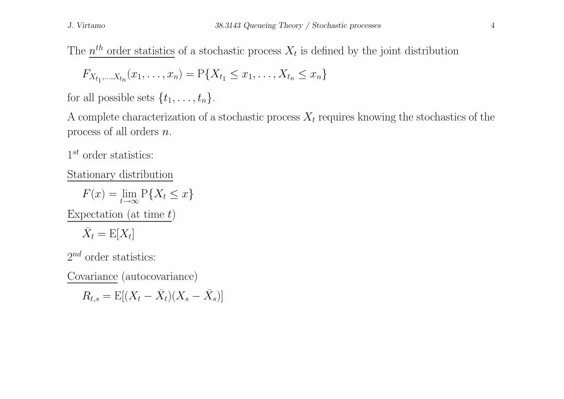
The nth order statistics of a stochastic process Xt is defined by the joint distribution

FXt1,...,Xtn

(x1, . . . , xn) = P{Xt1 ≤ x1, . . . , Xtn ≤ xn}

for all possible sets {t1, . . . , tn}.

A complete characterization of a stochastic process Xt requires knowing the stochastics of the

process of all orders n.

1st order statistics:

Stationary distribution

F (x) = limt→∞

P{Xt ≤ x}

Expectation (at time t)

X̄t = E[Xt]

2nd order statistics:

Covariance (autocovariance)

Rt,s = E[(Xt − X̄t)(Xs − X̄s)]

J. Virtamo 38.3143 Queueing Theory / Stochastic processes 5

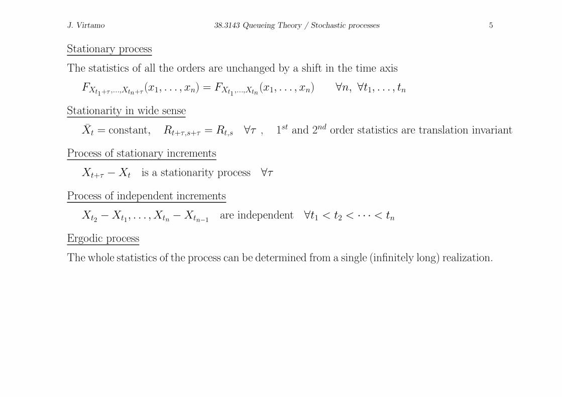
Stationary process

The statistics of all the orders are unchanged by a shift in the time axis

FXt1+τ ,...,Xtn+τ(x1, . . . , xn) = FXt1

,...,Xtn(x1, . . . , xn) ∀n, ∀t1, . . . , tn

Stationarity in wide sense

X̄t = constant, Rt+τ,s+τ = Rt,s ∀τ , 1st and 2nd order statistics are translation invariant

Process of stationary increments

Xt+τ − Xt is a stationarity process ∀τ

Process of independent increments

Xt2 − Xt1, . . . , Xtn − Xtn−1are independent ∀t1 < t2 < · · · < tn

Ergodic process

The whole statistics of the process can be determined from a single (infinitely long) realization.

J. Virtamo 38.3143 Queueing Theory / Stochastic processes 6

Markov process

A stochastic process is called a Markov process when it has the Markov property:

P{Xtn ≤ xn |Xtn−1= xn−1, . . .Xt1 = x1} = P{Xtn ≤ xn |Xtn−1

= xn−1} ∀n, ∀t1 < · · · < tn

• The future path of a Markov process, given its current state (Xtn−1) and the past history

before tn−1, depends only on the current state (not on how this state has been reached).

• The current state contains all the information (summary of the past) that is needed to

characterize the future (stochastic) behaviour of the process.

• Given the state of the process at an instant its future and past are independent.

Example A process with independent increments is always a Markov process.

Xtn = Xtn−1+ (Xtn − Xtn−1

)︸ ︷︷ ︸

the increment is independent of

all the previous increments which

have given rise to the state Xtn−1

J. Virtamo 38.3143 Queueing Theory / Stochastic processes 7

Markov chain

The use of the term Markov chain in the literature is ambiguous: it defines that the process

is either a discrete time or a discrete state process.

In the sequel, we limit the use of the term for the case where the process is both discrete time

and discrete state.

• Without loss of generality we can index the discrete instants of time by integers.

– A Markov chain is thus a process Xn, n = 0, 1, . . ..

• Similarly we can denote the states of the system by integers Xn = 0, 1, . . . (the set of

states can be finite or countably finite).

In the following we additionally assume that the process is time homogeneous.

A Markov process of this kind is characterized by the (one-step) transition probabilities

(transition from state i to state j):

pi,j = P{Xn = j |Xn−1 = i}time homogeneity: the transition probability does

not depend on n

J. Virtamo 38.3143 Queueing Theory / Stochastic processes 8

The probability of a path

The probability of a path i0, i1, . . . , in is

P{X0 = i0, . . . , Xn = in} = P{X0 = i0} pi0,i1 pi1,i2 · · · pin−1,in

Proof

P{X0 = i0, X1 = i1} = P{X1 = i1 |X0 = i0}︸ ︷︷ ︸

pi0,i1

P{X0 = i0}

P{X0 = i0, X1 = i1, X2 = i2} = P{X2 = i2 |X1 = i1, X0 = i0}︸ ︷︷ ︸

pi1,i2

P{X1 = i1, X0 = i0}︸ ︷︷ ︸

pi0,i1P{X0 = i0}= P{X0 = i0} pi0,i1 pi1,i2

Similarly, the proof can be continued for longer sequences.

P{X0 = i0} ↘i0•︸ ︷︷ ︸

pi0,i1

i1•︸ ︷︷ ︸

pi1,i2

i2•︸ ︷︷ ︸

pi2,i3

i3• · · ·

J. Virtamo 38.3143 Queueing Theory / Stochastic processes 9

The transition probability matrix of a Markov chain

The transition probabilities can be arranged as transition probability matrix P = (pi,j)

final state →

P =

p0,0 p0,1 p0,2 . . .

p1,0 p1,1 p1,2 . . .... ... ... . . .

↓ initial state

• The row i contains the transition probabilities from state i to other states.

– since the system always goes to some state, the sum of the row probabilities is 1

• A matrix with non-negative elements such that the sum of each row equals 1 is called a

stochastic matrix.

• One can easily show that the product of two stochastic matrices is a stochastic matrix.

J. Virtamo 38.3143 Queueing Theory / Stochastic processes 10

Many-step transition probability matrix

The probability that the system, initially in state i, will in

state j after two steps is∑

k

pi,kpk,j

(takes into account all paths via an intermediate state k).

i

k

j

Clearly this the element {i, j} of the matrix P2.

Similarly, one finds that the n-step transition probability matrix Pn.

Denote its elements by p(n)i,j (the subscript refers to the number of steps). Since it holds that

Pn = Pm · Pn−m (0 ≤ m ≤ n), we can write in component form

p(n)i,j =

∑

k

p(m)i,k p

(n−m)k,j the Chapman-Kolmogorov equation

This simply expresses the law of total probability, where the transition in n steps from state

i to state j is conditioned on the system being in state k after m steps.

J. Virtamo 38.3143 Queueing Theory / Stochastic processes 11

State probabilities

Denote

π(n)i = P{Xn = i} the probability that the process is in state i at time n

Arrange the state probabilities at time n in a state probability vector

π(n) = (π

(n)0 , π

(n)1 , π

(n)2 , . . .)

By the law of total probability we have

P{X1 = i} =∑

k

P{X1 = i |X0 = k}P{X0 = k}

or π(1)i =

∑

k π(0)k pk,i and in vector form π

(1) = π(0)P

As the process is Markovian and π(1) represents the initial probabilities in the next step,

π(2) = π

(1)P and generally π(n) = π

(n−1)P

from which we have recursively

π(n) = π

(0)Pn (Note, Pn is the n-step transition probability matrix.)

J. Virtamo 38.3143 Queueing Theory / Stochastic processes 12

Example

P =

1 − p p(1 − p) p2

1 − p p(1 − p) p2

0 1 − p p

p = 1/3

0

1

21-pp

2

p2

p

p(1-p)

p(1-p

)

1-p

1-p

P = 1

9

6 2 1

6 2 1

0 6 3

=

0.6666 0.2222 0.1111

0.6666 0.2222 0.1111

0 0.6666 0.3333

P2 = 1

92

48 22 11

48 22 11

36 30 15

=

0.5926 0.2716 0.1358

0.5926 0.2716 0.1358

0.4444 0.3704 0.1852

P3 = 1

93

420 206 103420 206 103

396 222 111

=

0.5761 0.2826 0.14130.5761 0.2826 0.1413

0.5432 0.3045 0.1523

...

P8 =

0.5714 0.2857 0.1429

0.5714 0.2857 0.1429

0.5714 0.2857 0.1429

Starting from an initial state i, the distribution of the final state can be read from the row i.

After 8 steps the final state distribution is independent of the initial state (to the accuracy of

four digits): “the process forgets its initial state”.

J. Virtamo 38.3143 Queueing Theory / Stochastic processes 13

Classification of states of a Markov chain

State i leads to state j (written i → j), if there is

a path i0 = i, i1, . . . , in = j such that all the tran-

sition probabilities are positive, pik,ik+1> 0, k =

0, . . . , n − 1.

Then (Pn)i,j > 0.

i1i2

i3

j=in

i=i0....

States i and j communicate (written i ↔ j), if

i → j and j → i.

i

j

Communication is an equivalence relation: the states can be grouped into equivalent classes

so that

• within each class all the states communicate with each other

• two states from two different classes never communicate which each other

The equivalence classes defined by the relation ↔ are called the irreducible classes of states

A Markov chain with a state space which is an irreducible class

(the only one, i.e. all the states communicate) is called irreducible.

J. Virtamo 38.3143 Queueing Theory / Stochastic processes 14

Classification of states (continued)

A set of states is closed, if none of its states leads to any of the states outside the set.

A single state which alone forms a closed set is called an absorbing state

- for an absorbing state we have pi,i = 1

- one may reach an absorbing state from other states, but one cannot get out of it

Each state is either transient or recurrent.

• A state i is transient if the probability of returning to the state is < 1.

i.e. there is a non-zero probability that the system never returns to the state.

• A state i is recurrent if the probability of returning to the state is = 1.

i.e. with certainty, the system sometimes returns to the state.

Recurrent states are further classified according to the expectation of the time Ti,i1 it takes

to return to the state:

positive recurrent

expectation of first return time < ∞

null recurrent

expectation of first return time = ∞

1The first return time Ti,i of state i is the time at which the Markov chain first returns to state i whenX0 = i.

J. Virtamo 38.3143 Queueing Theory / Stochastic processes 15

Classification of states (continued)

Type # of visits E[Ti,i]

Transient < ∞ ∞

Null recurrent ∞ ∞

Positive recurrent ∞ < ∞

If the first return time of state i can only be a multiple of an integer d > 1 the state i is called

periodic. Otherwise the state is aperiodic.

An aperiodic positive recurrent state is ergodic

A Markov chain is ergodic, iff all its states are ergodic.

0 1 2

3 4

6 7

n 8

5

. . .

absorboiva transientti

jaksollinen

jaksotonpositiivisestipalautuva

J. Virtamo 38.3143 Queueing Theory / Stochastic processes 16

Classification of states (continued)

Proposition: In an irreducible Markov chain either

- all the states are transient, or

- all the states are null recurrent, or

- all the states are positive recurrent

Remarks on the life time of a state and the first return time

The number of steps the system consecutively

stays in state i is geometrically distributed

∼ Geom(1 − pi,i)

because the exit from the state occurs with the

probability 1 − pi,i.

íî

ìi

pi, i

1- pi, i

After each visit of state i, the first return time Ti,i back to state i is independent of the first

return times after any of the other visits to the state (follows from the Markov property).

Denote T̄i = E[Ti,i] T̄i =

∞ if the state is transient or null recurrent

< ∞ if the state is positive recurrent

J. Virtamo 38.3143 Queueing Theory / Stochastic processes 17

Kolmogorov’s theorem

In an irreducible, aperiodic Markov chain there always exist the limits

πj = limn→∞

π(n)j = 1/T̄j

and these are independent of the initial state.

Furthermore, either

i) all the states of the chain are transient or all of the states are null recurrent; in either

case πj = 0, ∀j,

or

ii) all the states of the chain are positive recurrent, and there exists a unique stationary

distribution π which is obtained as the solution of the equations

π = π · P

π · eT = 1or

πj =∑

iπi pi,j and

∑

jπj = 1

(e is a row vector with all the components equal to 1, and

eT is the corresponding column vector)

J. Virtamo 38.3143 Queueing Theory / Stochastic processes 18

Remarks on the stationary distribution

If the limit probabilities (the components of the vector) π exist, they must satisfy the equation

π = πP, because

π = limn→∞

π(n) = lim

n→∞π

(n+1) = limn→∞

π(n) · P = πP

The equation π = πP can also be expressed in the form: π is the (left) eigenvector of the

matrix P belonging to the eigenvalue 1 (or belonging to the eigenvalue 0 of the matrix (P−I)).

πj defines which proportion of time (steps) the system stays in state j.

The limit distribution π is called the stationary distribution or the equilibrium distribution

Note. An equilibrium does not mean that nothing happens in the system, but merely that

the information on the initial state of the system has been “forgot” or “washed out” because

of the stochastic development.

J. Virtamo 38.3143 Queueing Theory / Stochastic processes 19

Global balance

Equation π = πP or πj =∑

iπi pi,j, ∀j, is often called the (global) balance condition.

Since∑

ipj,i = 1 (the transition takes the system to some state), one can write

∑

iπj pj,i

︸ ︷︷ ︸

prob. that the system is in

state j and makes a transi-

tion to another state

=∑

iπi pi,j

︸ ︷︷ ︸

prob. that the system is in

another state and makes a

transition to state j

One equation for each state j.

Balance of probability flows: there

are as many exits form state j as

there are entries to it.

S S

j j

=

• If the balance equations are known to be satisfied for all but one of the states, they are

automatically satisfied also for that particular state (due to conservation of probability

flows)

• – the balance equations are linearly dependent

(⇒ the homogeneous equation π = πP has a non-zero solution)

– the solution is determined up to a constant factor

– in order to determine the unknown factor, one needs the normalization condition∑

j πj = 1

J. Virtamo 38.3143 Queueing Theory / Stochastic processes 20

Example. We revisit the previous example (now with a general p).

( π0 π1 π2 ) = ( π0 π1 π2 )

1 − p p(1 − p) p2

1 − p p(1 − p) p2

0 1 − p p

Write the first two equations (equalities of the first two components of the vectors on the lhs

and rhs)

π0 = (1 − p)π0 + (1 − p)π1 ⇒ π0 = 1−pp

π1

π1 = p(1 − p)π0 + p(1 − p)π1 + (1 − p)π2

= (1 − p)2π1 + p(1 − p)π1 + (1 − p)π2

= (1 − p)π1 + (1 − p)π2 ⇒ π1 = 1−pp

π2 ⇒ π0 =(

1−pp

)2π2

or

π =( (

1−pp

)2 1−pp

1)

π2 .

By the normalization condition π0 + π1 + π2 = 1 one gets

π =(

(1−p)2

1−p(1−p)p(1−p)

1−p(1−p)p2

1−p(1−p)

)

With p = 13

: π = ( 0.5714 0.2857 0.1429 )

J. Virtamo 38.3143 Queueing Theory / Stochastic processes 21

On solving the balance (or equilibrium) equations

In general, the equilibrium equations are solved as follows (assume a finite state space with n

states):

• Write the balance condition for all but one of the states (n − 1 equations)

– the equations fix the relative values of the equilibrium probabilities

– the solution is determined up to a constant factor

• The last balance equation (automatically satisfied) is replaced by the normalization con-

dition∑

j πj = 1.

For calculation by a computer, it’s often more convenient to use the following method

(usually, one construct the whole transition probability matrix P):

Write n copies of the normalization condition π · eT = 1:

π · E = e where E is an n× n-matrix with all the elements equal to 1, E =

1 1 . . . 1

.

.

.

.

.

.

...

.

.

.

1 1 . . . 1

Add this equation and the balance equation π · P = π ⇒ π · (P + E − I) = e

π = e · (P + E− I)−1The inhomogeneous equation has a unique solution.

The solution automatically satisfies both the balance and

the normalization conditions.