53
Stochastic processes Lecture 6 Power spectral density (PSD) 1
| Date post: | 18-Dec-2015 |
| Category: |
Documents |
| Upload: | cory-collins |
| View: | 229 times |
| Download: | 2 times |
1
Stochastic processes
Lecture 6Power spectral density (PSD)
2
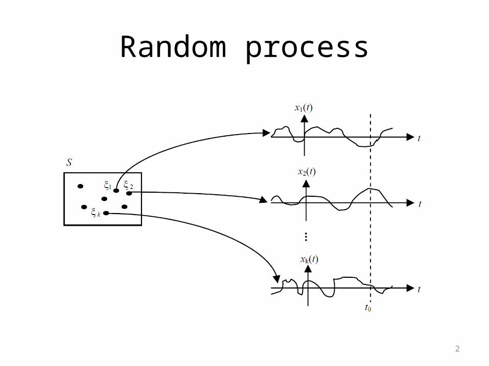
Random process
3
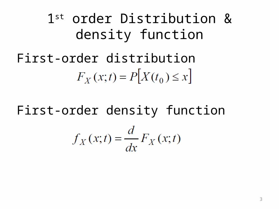
1st order Distribution & density function
First-order distribution
First-order density function

4
2end order Distribution & density function
2end order distribution
2end order density function
5
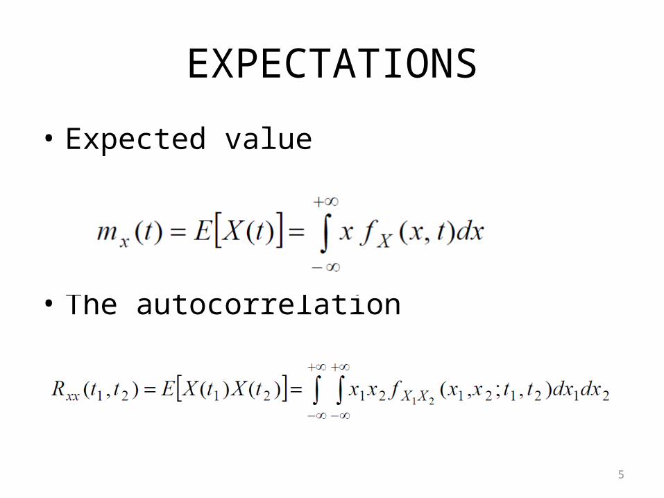
EXPECTATIONS
• Expected value
• The autocorrelation

6
Some random processes
• Single pulse• Multiple pulses• Periodic Random Processes• The Gaussian Process• The Poisson Process• Bernoulli and Binomial Processes• The Random Walk Wiener Processes• The Markov Process
7
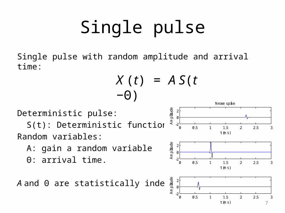
Single pulse
Single pulse with random amplitude and arrival time:
Deterministic pulse: S(t): Deterministic function. Random variables:
A: gain a random variable Θ: arrival time.
A and Θ are statistically independent
X (t) = A S(t −Θ)
0 0.5 1 1.5 2 2.5 3-2
0
2
t (ms)
Am
plitu
de
Nerve spike
0 0.5 1 1.5 2 2.5 3-2
0
2
t (ms)A
mpl
itude
0 0.5 1 1.5 2 2.5 3-2
0
2
Am
plitu
de
t (ms)
8
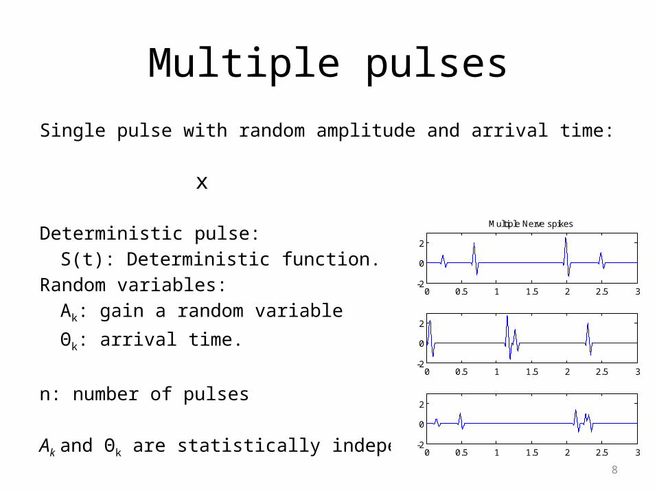
Multiple pulsesSingle pulse with random amplitude and arrival time:
Deterministic pulse: S(t): Deterministic function. Random variables:
Ak: gain a random variable
Θk: arrival time.
n: number of pulses
Ak and Θk are statistically independent
x
0 0.5 1 1.5 2 2.5 3-2
0
2
Multiple Nerve spikes
0 0.5 1 1.5 2 2.5 3-2
0
2
0 0.5 1 1.5 2 2.5 3-2
0
2
9
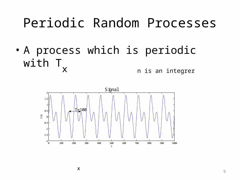
Periodic Random Processes
• A process which is periodic with T
x n is an integrer
x
0 100 200 300 400 500 600 700 800 900 1000-2
-1.5
-1
-0.5
0
0.5
1
1.5
2
t
X(t
)
Signal
T=100
10
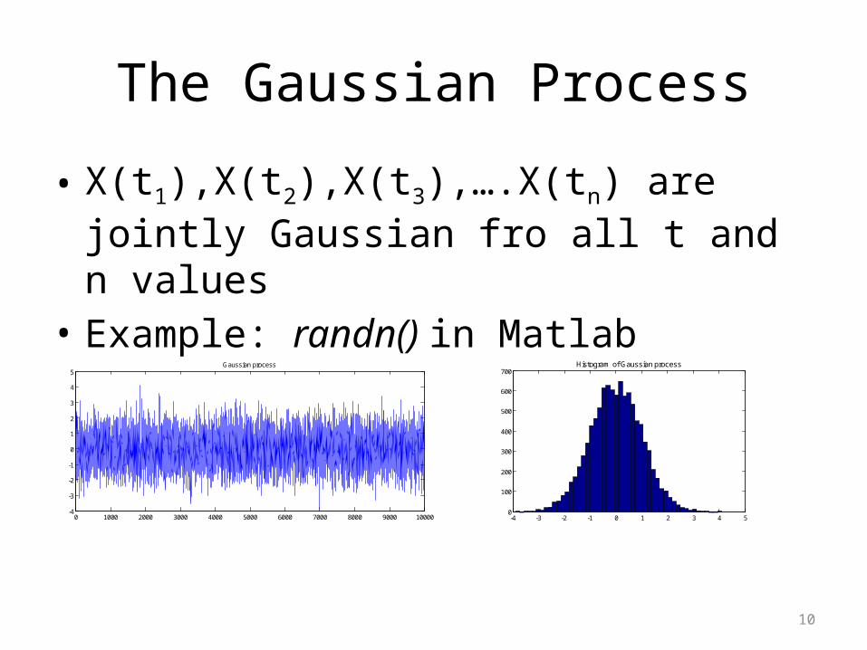
The Gaussian Process
• X(t1),X(t2),X(t3),….X(tn) are jointly Gaussian fro all t and n values
• Example: randn() in Matlab
0 1000 2000 3000 4000 5000 6000 7000 8000 9000 10000-4
-3
-2
-1
0
1
2
3
4
5Gaussian process
-4 -3 -2 -1 0 1 2 3 4 50
100
200
300
400
500
600
700Histogram of Gaussian process
11
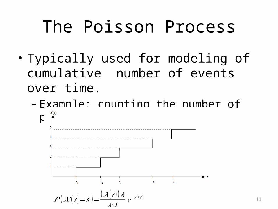
The Poisson Process
• Typically used for modeling of cumulative number of events over time.– Example: counting the number of phone call from
a phone
𝑃 (𝑋 (𝑡 )=𝑘 )= (𝜆 (𝑡 ) )𝑘𝑘!
𝑒−𝜆(𝑡 )
12
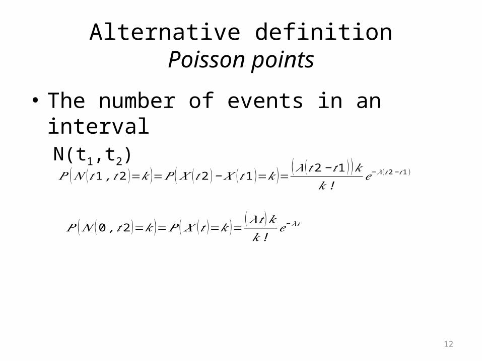
Alternative definitionPoisson points
• The number of events in an intervalN(t1,t2)
𝑃 (𝑁 (0 ,𝑡 2 )=𝑘 )=𝑃 ( 𝑋 (𝑡 )=𝑘 )= (𝜆𝑡 )𝑘𝑘!
𝑒−𝜆𝑡
𝑃 (𝑁 (𝑡 1 ,𝑡 2 )=𝑘 )=𝑃 (𝑋 (𝑡 2 )−𝑋 (𝑡 1 )=𝑘)= (𝜆 (𝑡 2−𝑡 1 ) )𝑘𝑘!
𝑒−𝜆(𝑡2−𝑡 1)
13
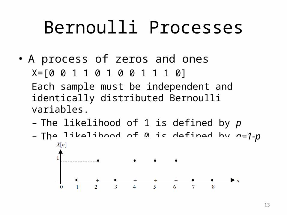
Bernoulli Processes
• A process of zeros and onesX=[0 0 1 1 0 1 0 0 1 1 1 0]Each sample must be independent and identically distributed Bernoulli variables.– The likelihood of 1 is defined by p – The likelihood of 0 is defined by q=1-p
14
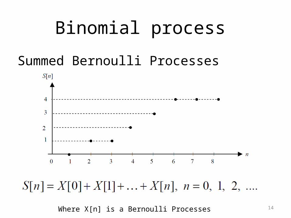
Binomial process
Summed Bernoulli Processes
Where X[n] is a Bernoulli Processes

15
Random walk
• For every T seconds take a step (size Δ) to the left or right after tossing a fair coin
0 5 10 15 20 25 30 35 40 45 50-8
-6
-4
-2
0
2
4
6
n
x[n]
Random walks
16
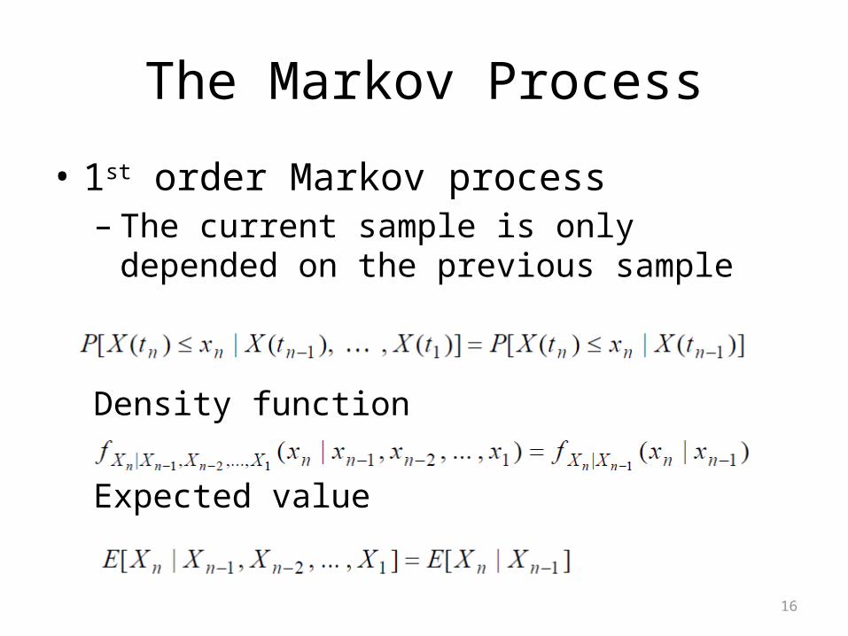
The Markov Process
• 1st order Markov process– The current sample is only depended on the
previous sample
Density function
Expected value

17
The frequency of earth quakes
• Statement the number large earth quakes has increased dramatically in the last 10 year!

18
The frequency of earth quakes
• Is the frequency of large earth quakes unusual high?
• Which random processes can we use for modeling of the earth quakes frequency?

19
The frequency of earth quakes
• Data• http://
earthquake.usgs.gov/earthquakes/eqarchives/year/graphs.php

20
Agenda (Lec 16)
• Power spectral density– Definition and background– Wiener-Khinchin– Cross spectral densities– Practical implementations– Examples
21
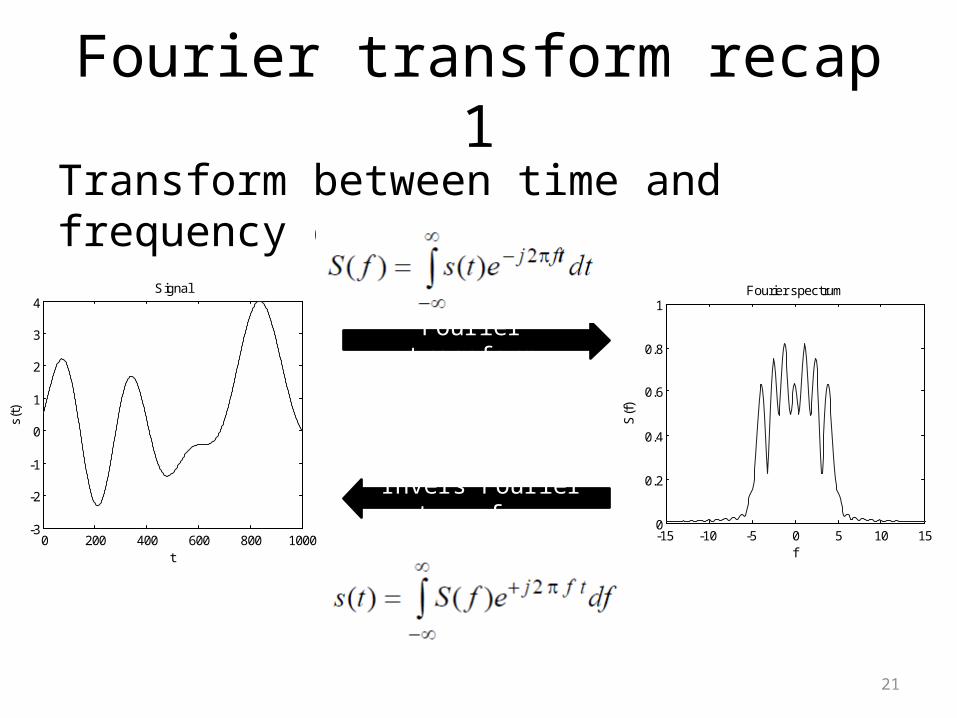
Fourier transform recap 1Transform between time and frequency domain
Fourier transform
Invers Fourier transform0 200 400 600 800 1000
-3
-2
-1
0
1
2
3
4Signal
s(t)
t
-15 -10 -5 0 5 10 150
0.2
0.4
0.6
0.8
1
S(f
)
f
Fourier spectrum

22
Fourier transform recap 2
• Assumption: The signal can be reconstructed from sines and cosines functions.
• Requirement: absolute integrable
𝑒− 𝑗 2𝜋 𝑓𝑡=cos (2𝜋 𝑓𝑡 )− 𝑗 sin (2𝜋 𝑓𝑡 )0 20 40 60 80 100
-1
-0.5
0
0.5
1
nA
mpl
itude
e(jw n)
Real
Imaginary
n
nx ][
23
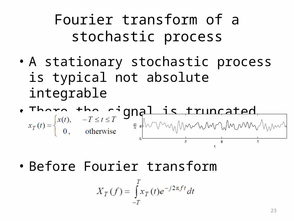
Fourier transform of a stochastic process
• A stationary stochastic process is typical not absolute integrable
• There the signal is truncated
• Before Fourier transform-T 0 T
-5
0
5
t
x(t)
24
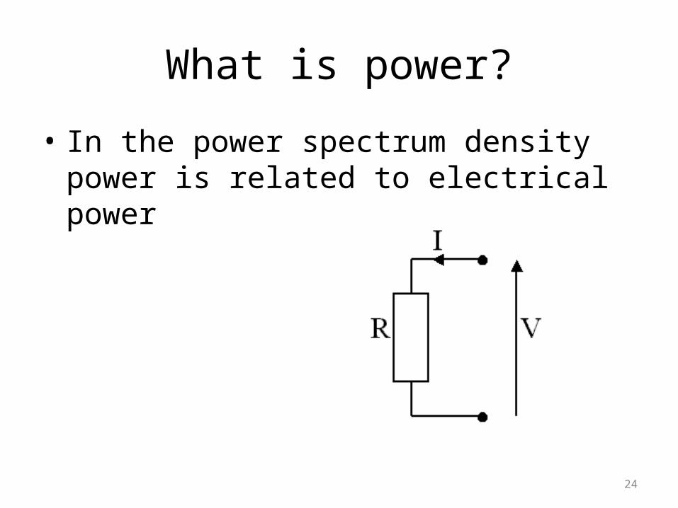
What is power?
• In the power spectrum density power is related to electrical power

25
Power of a signal
• The power of a signal is calculated by squaring the signal.
• The average power in e period is :
26
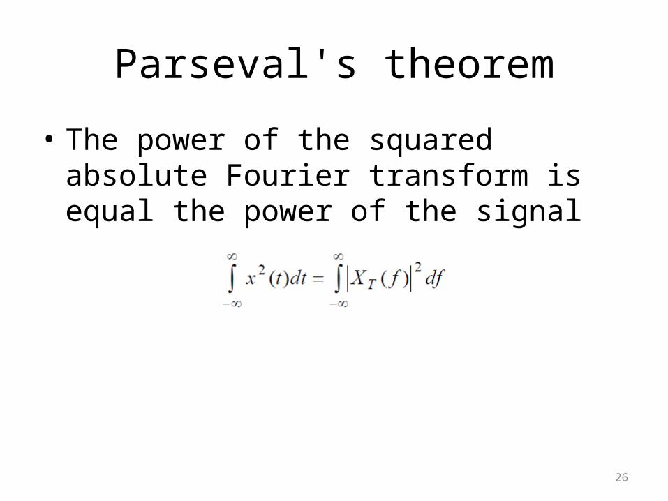
Parseval's theorem
• The power of the squared absolute Fourier transform is equal the power of the signal
27
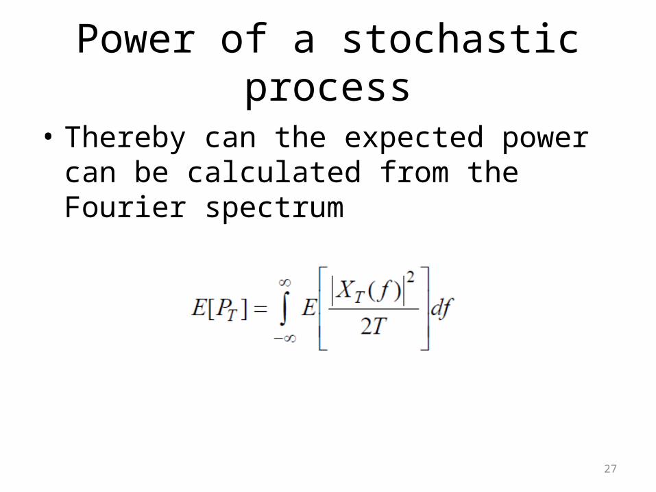
Power of a stochastic process
• Thereby can the expected power can be calculated from the Fourier spectrum
28
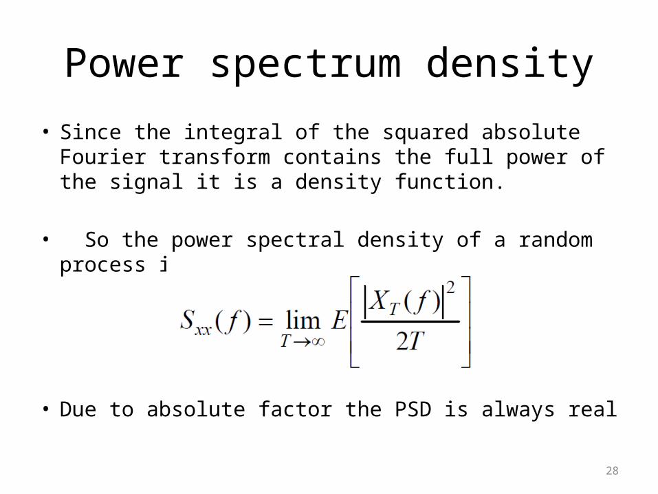
Power spectrum density
• Since the integral of the squared absolute Fourier transform contains the full power of the signal it is a density function.
• So the power spectral density of a random process is:
• Due to absolute factor the PSD is always real

29
PSD Example
-15 -10 -5 0 5 10 150
0.2
0.4
0.6
0.8
1
Sxx
(f)
f
PSD
Fourier transform
0 200 400 600 800 1000-3
-2
-1
0
1
2
3
4Signal
s(t)
t
-15 -10 -5 0 5 10 150
0.2
0.4
0.6
0.8
1
S(f
)
f
Fourier spectrum
|X(f)|2
30
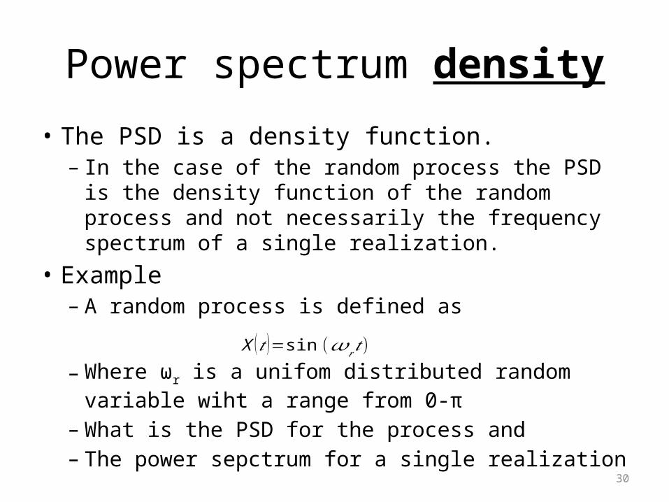
Power spectrum density
• The PSD is a density function.– In the case of the random process the PSD is the density
function of the random process and not necessarily the frequency spectrum of a single realization.
• Example– A random process is defined as
– Where ωr is a unifom distributed random variable wiht a range from 0-π
– What is the PSD for the process and – The power sepctrum for a single realization
X (𝑡 )=sin (𝜔𝑟 𝑡)
31
PSD of random process versus spectrum of deterministic signals
• In the case of the random process the PSD is usual the expected value E[Sxx(f)]
• In the case of deterministic signals the PSD is exact (There is still estimation error)

32
Properties of the PSD
1. Sxx(f) is real and nonnegative
2. The average power in X(t) is given by:
3. If X(t) is real Rxx(τ) and Sxx(f) are also even
4. If X(t) has periodic components Sxx(f)has impulses
5. Independent on phase
33
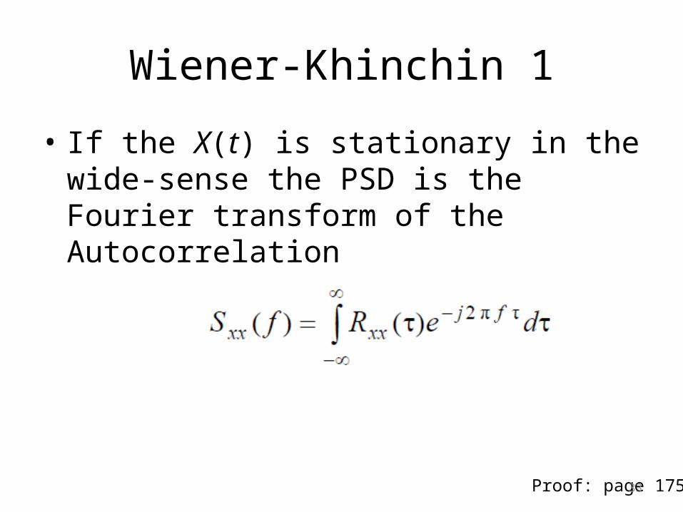
Wiener-Khinchin 1
• If the X(t) is stationary in the wide-sense the PSD is the Fourier transform of the Autocorrelation
Proof: page 175

34
Wiener-Khinchin Two method for estimation of the PSD
X(t)
Fourier Transform
|X(f)|2
Sxx(f)
Autocorrelation
Fourier Transformt
X(t
)
f
X(f
)
Rxx
()
f
Sxx
(f)

35
The inverse Fourier Transform of the PSD
• Since the PSD is the Fourier transformed autocorrelation
• The inverse Fourier transform of the PSD is the autocorrelation
36
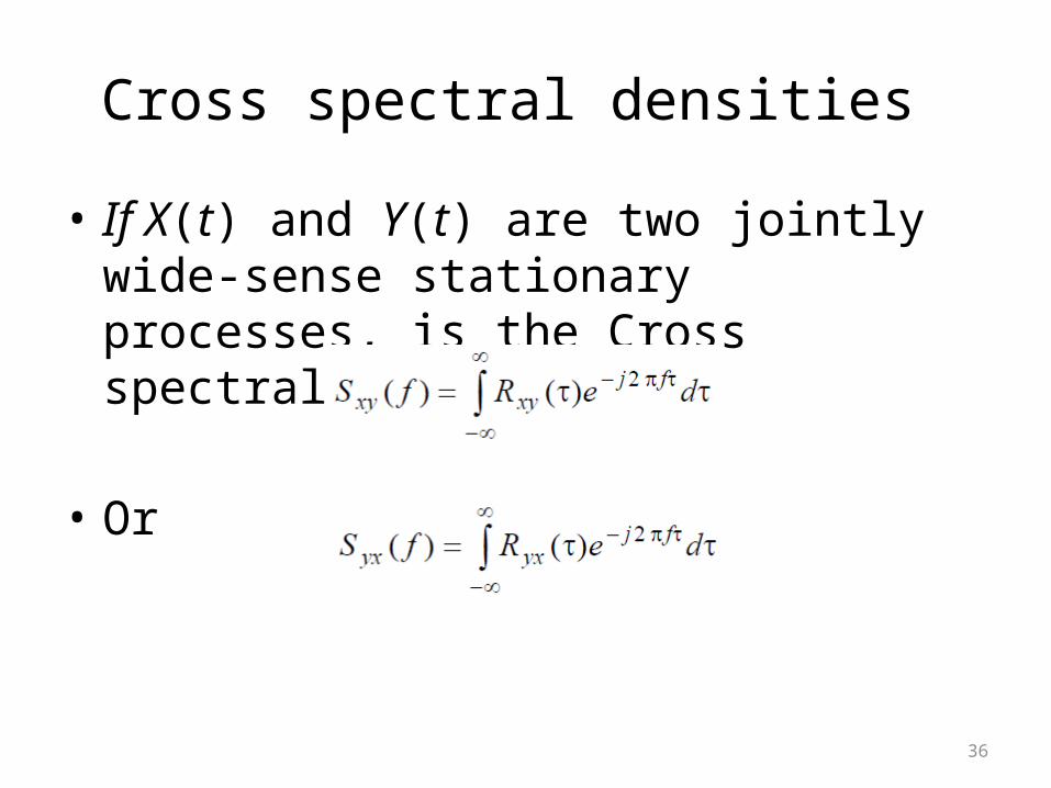
Cross spectral densities
• If X(t) and Y(t) are two jointly wide-sense stationary processes, is the Cross spectral densities
• Or

37
Properties of Cross spectral densities
1. Since is
2. Syx(f) is not necessary real
3. If X(t) and Y(t) are orthogonal Sxy(f)=0
4. If X(t) and Y(t) are independent Sxy(f)=E[X(t)] E[Y(t)] δ(f)

38
Cross spectral densities example
• 1 Hz Sinus curves in white noise
Where w(t) is Gaussian noise
0 5 10 15 20-10
0
10
X(t
)
t (s)
Signal X(t)
0 5 10 15 20-10
0
10
Y(t
)
t (s)
Signal Y(t)
𝑋 (𝑡 )=sin (2𝜋 𝑡 )+3𝑤 (𝑡)𝑌 (𝑡 )=sin(2𝜋𝑡+𝜋2 )+3𝑤(𝑡)
0 5 10 15 20 25-30
-25
-20
-15
-10
-5
0
5
Frequency (Hz)
Pow
er/f
requ
ency
(dB
/Hz)
Welch Cross Power Spectral Density Estimate
39
Implementations issues
• The challenges includes– Finite signals – Discrete time

40
The periodogramThe estimate of the PSD
• The PSD can be estimate from the autocorrelation
• Or directly from the signal
𝑆 𝑥𝑥 [ω ]= ∑𝑚=−𝑁+1
𝑁− 1
𝑅𝑥𝑥 [𝑚]𝑒− 𝑗 ω𝑚
𝑆 𝑥𝑥 [ω ]= 1𝑁 |∑
𝑛=0
𝑁− 1
𝑥 [𝑛]𝑒− 𝑗ω𝑛 |2
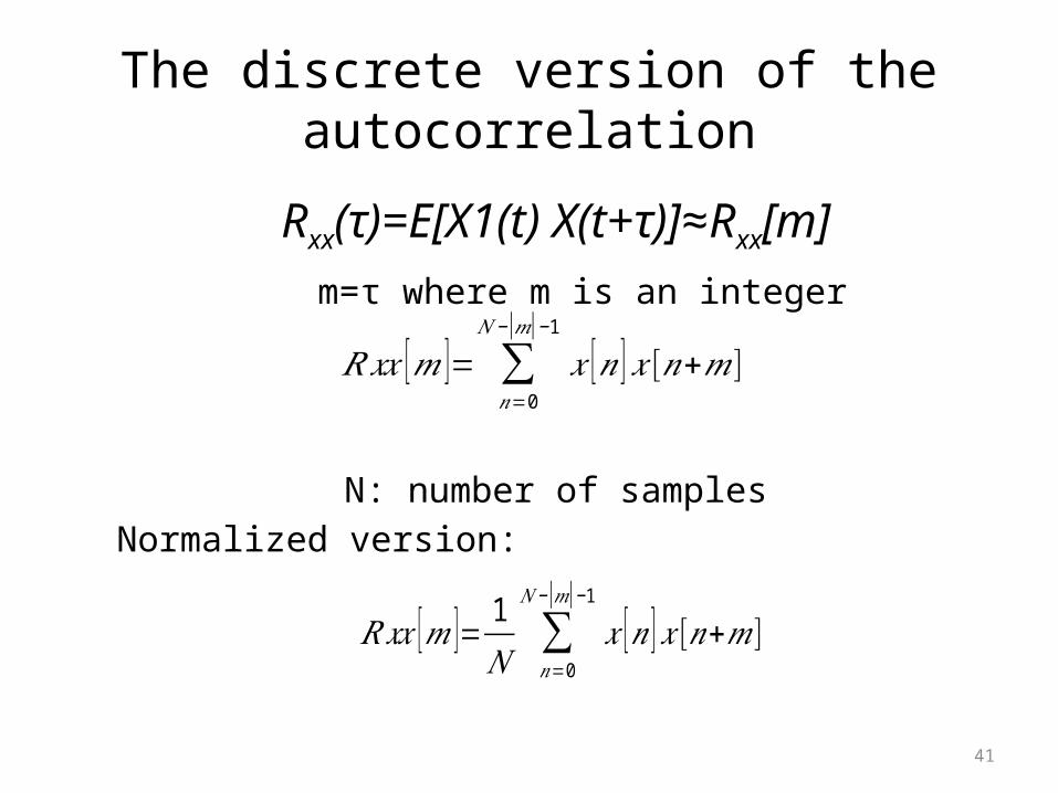
41
The discrete version of the autocorrelation
Rxx(τ)=E[X1(t) X(t+τ)]≈Rxx[m]m=τ where m is an integer
N: number of samplesNormalized version:
𝑅𝑥𝑥 [𝑚 ]= ∑𝑛=0
𝑁−|𝑚|− 1
𝑥 [𝑛 ] 𝑥 [𝑛+𝑚]
𝑅𝑥𝑥 [𝑚 ]= 1𝑁 ∑
𝑛=0
𝑁−|𝑚|−1
𝑥 [𝑛 ] 𝑥[𝑛+𝑚 ]

42
Bias in the estimates of the autocorrelation
N=12𝑅𝑥𝑥 [𝑚 ]= ∑
𝑛=0
𝑁−|𝑚|− 1
𝑥 [𝑛 ] 𝑥 [𝑛+𝑚]
-10 -5 0 5 10 15 20-2
-1
0
1
2
n
-10 -5 0 5 10 15 20-2
-1
0
1
2
n+m-15 -10 -5 0 5 10 15
-6
-4
-2
0
2
4
6
8Autocorrelation
M=-10
-10 -5 0 5 10 15 20-2
-1
0
1
2
n
-10 -5 0 5 10 15 20-2
-1
0
1
2
n+m-15 -10 -5 0 5 10 15
-6
-4
-2
0
2
4
6
8Autocorrelation
M=0
-10 -5 0 5 10 15 20-2
-1
0
1
2
n
-10 -5 0 5 10 15 20-2
-1
0
1
2
n+m-15 -10 -5 0 5 10 15
-6
-4
-2
0
2
4
6
8Autocorrelation
M=4
43
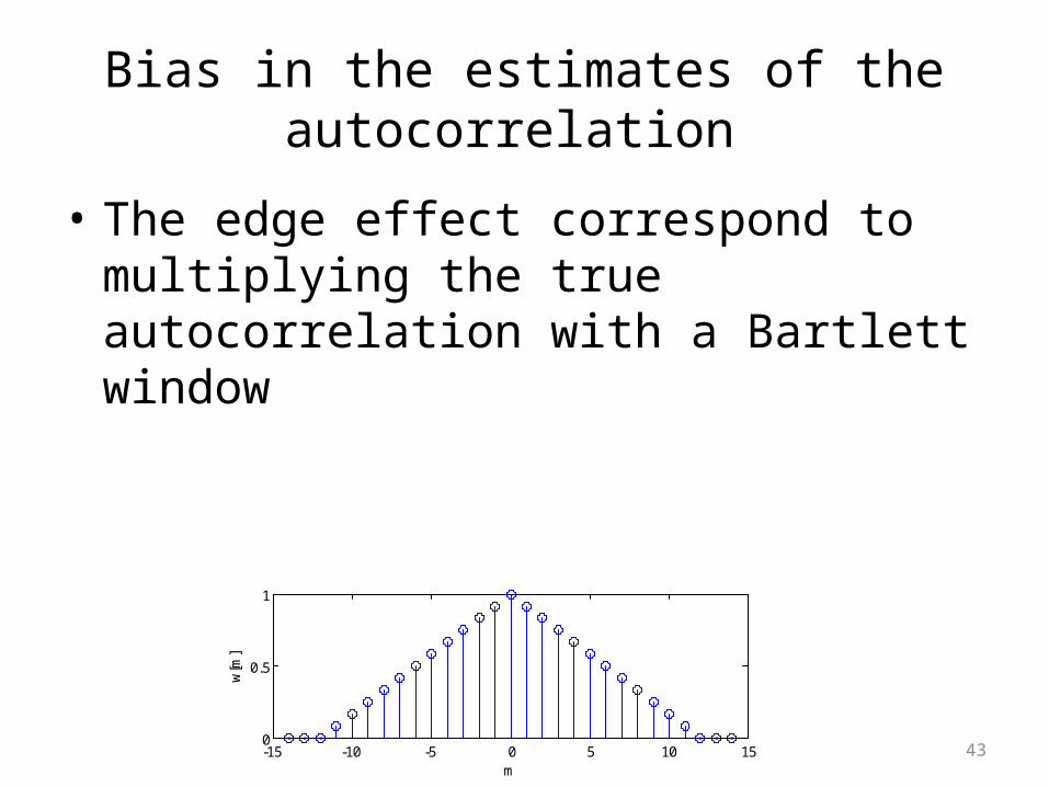
Bias in the estimates of the autocorrelation
• The edge effect correspond to multiplying the true autocorrelation with a Bartlett window
-15 -10 -5 0 5 10 150
0.5
1
m
w[m
]

44
Alternative estimation of autocorrelation
• The unbiased estimate
• Disadvantage: high variance when |m|→N
𝑅𝑥𝑥 [𝑚 ]= 1
𝑁−∨𝑚∨¿ ∑𝑛=0
𝑁 −|𝑚|−1
𝑥 [𝑛 ] 𝑥 [𝑛+𝑚]¿
-15 -10 -5 0 5 10 15
-0.6
-0.4
-0.2
0
0.2
0.4
0.6
Rxx
[m]
m
Biased
-15 -10 -5 0 5 10 15
-0.6
-0.4
-0.2
0
0.2
0.4
0.6
Rxx
[m]
m
Unbiased

45
Influence at the power spectrum
• Biased version: a Bartlett window is applied
• Unbiased version: a Rectangular window is applied
𝑆 𝑥𝑥 [ω ]= ∑𝑚=−∞
∞
𝑤𝑏 [𝑚 ]𝑅𝑥𝑥𝑢𝑛𝑏𝑖𝑎𝑠𝑒𝑑 [𝑚 ]𝑒− 𝑗ω𝑚
𝑤𝑟 [𝑚 ]={1 |𝑚|<𝑁0 h𝑜𝑡 𝑒𝑟𝑤𝑖𝑠𝑒
46
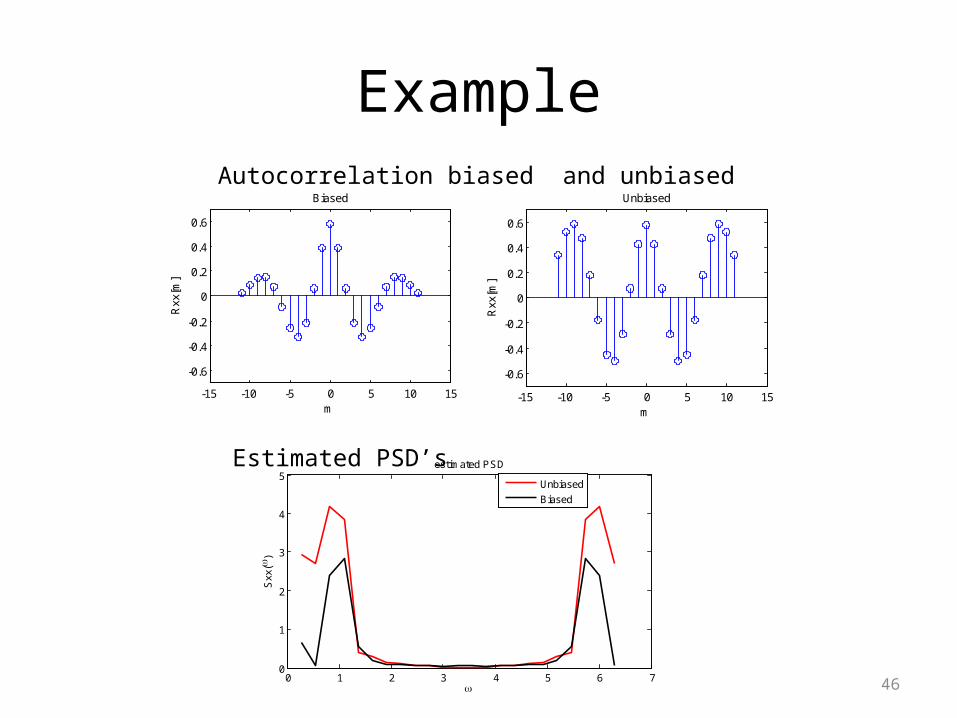
Example
0 1 2 3 4 5 6 70
1
2
3
4
5
Sxx
()
estimated PSD
Unbiased
Biased
-15 -10 -5 0 5 10 15
-0.6
-0.4
-0.2
0
0.2
0.4
0.6
Rxx
[m]
m
Biased
-15 -10 -5 0 5 10 15
-0.6
-0.4
-0.2
0
0.2
0.4
0.6
Rxx
[m]
m
Unbiased
Autocorrelation biased and unbiased
Estimated PSD’s
47
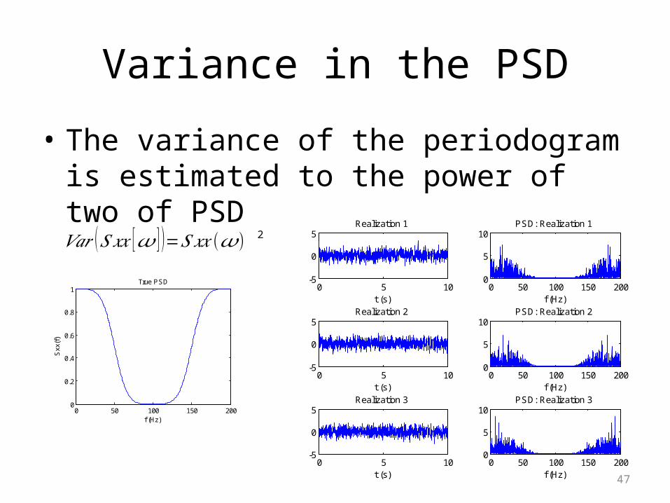
Variance in the PSD
• The variance of the periodogram is estimated to the power of two of PSD
𝑉𝑎𝑟 (𝑆𝑥𝑥 [𝜔 ] )=𝑆 𝑥𝑥(𝜔) 2
0 5 10-5
0
5Realization 1
t (s)0 50 100 150 200
0
5
10PSD: Realization 1
f (Hz)
0 5 10-5
0
5
t (s)
Realization 2
0 50 100 150 2000
5
10
f (Hz)
PSD: Realization 2
0 5 10-5
0
5
t (s)
Realization 3
0 50 100 150 2000
5
10
f (Hz)
PSD: Realization 3 0 50 100 150 200
0
0.2
0.4
0.6
0.8
1
f (Hz)
Sxx
(f)
True PSD
48
Averaging
• Divide the signal into K segments of M length
• Calculate the periodogram of each segment
• Calculate the average periodogram
49
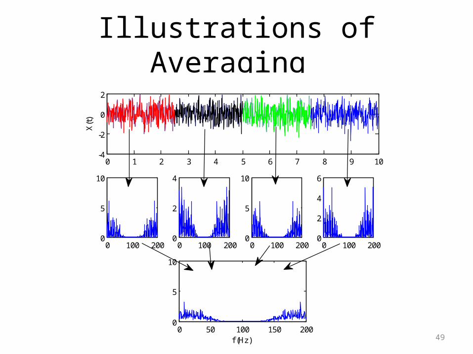
Illustrations of Averaging
0 1 2 3 4 5 6 7 8 9 10-4
-2
0
2X
(t)
0 100 2000
5
10
0 100 2000
2
4
0 100 2000
5
10
0 100 2000
2
4
6
0 50 100 150 2000
5
10
f (Hz)
50
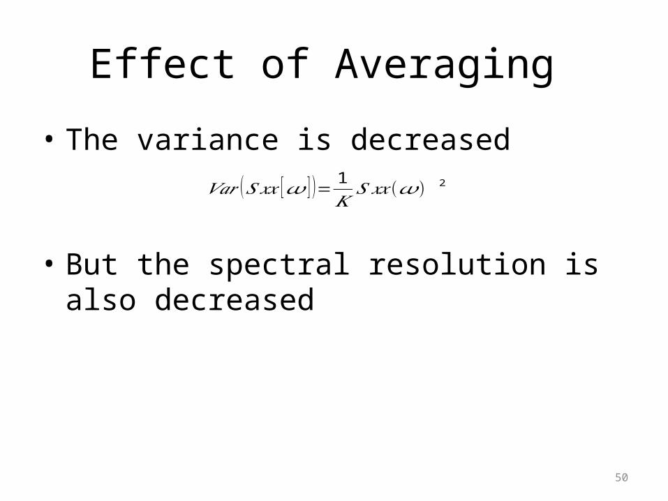
Effect of Averaging
• The variance is decreased
• But the spectral resolution is also decreased
𝑉𝑎𝑟 (𝑆𝑥𝑥 [𝜔 ] )= 1𝐾𝑆𝑥𝑥 (𝜔 ) 2
51
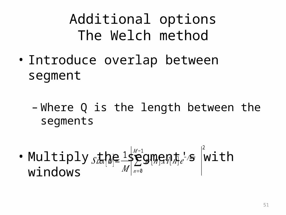
Additional optionsThe Welch method
• Introduce overlap between segment
– Where Q is the length between the segments
• Multiply the segment's with windows
𝑆𝑖𝑥𝑥 [ω ]= 1𝑀 |∑
𝑛=0
𝑀−1
𝑤 [𝑛]𝑥 𝑖[𝑛]𝑒− 𝑗ω𝑛 |2
52
Example
• Heart rate variability
• http://circ.ahajournals.org/cgi/content/full/93/5/1043#F3
• High frequency component related to Parasympathetic nervous system ("rest and digest")
• Low frequency component related to sympathetic nervous system (fight-or-flight)

53
Agenda (Lec 16)
• Power spectral density– Definition and background– Wiener-Khinchin– Cross spectral densities– Practical implementations– Examples


