Stochastic volatility: option pricing using a multinomial recombining tree Ionut ¸ Florescu 1,3 and Frederi G. Viens 2,4 1 Department of Mathematical Sciences, Stevens Institute of Technology, Castle Point on the Hudson, Hoboken, NJ 07030 2 Department of Statistics, Purdue University, 150 N. University St, West Lafayette, IN 47907-2067 3 [email protected]4 [email protected]Abstract We treat the problem of option pricing under the Stochastic Volatility (SV) model: the volatility of the underlying asset is a function of an exogenous stochastic process, typically assumed to be mean- reverting. Assuming that only discrete past stock information is available, we adapt an interacting particle stochastic filtering algorithm due to Del Moral, Jacod and Protter (Del Moral et al., 2001) to estimate the SV, and construct a quadrinomial tree which samples volatilities from the SV filter’s empirical measure approximation at time 0. Proofs of convergence of the tree to continuous-time SV models are provided. Classical arbitrage-free option pricing is performed on the tree, and provides answers that are close to market prices of options on the SP500 or on blue-chip stocks. We compare our results to non-random volatility models, and to models which continue to estimate volatility after time 0. We show precisely how to calibrate our incomplete market, choosing a specific martingale measure, by using a benchmark option. Key words and phrases: incomplete markets, Monte-Carlo method, options market, option pricing, particle method, random tree, stochastic filtering, stochastic volatility. 1
Transcript
Stochastic volatility: option pricing using a multinomial
recombining tree
Ionut Florescu1,3 and Frederi G. Viens2,4
1Department of Mathematical Sciences, Stevens Institute of Technology,
Castle Point on the Hudson, Hoboken, NJ 07030
2Department of Statistics, Purdue University,
150 N. University St, West Lafayette, IN 47907-2067
We treat the problem of option pricing under the Stochastic Volatility (SV) model: the volatility
of the underlying asset is a function of an exogenous stochastic process, typically assumed to be mean-
reverting. Assuming that only discrete past stock information is available, we adapt an interacting particle
stochastic filtering algorithm due to Del Moral, Jacod and Protter (Del Moral et al., 2001) to estimate the
SV, and construct a quadrinomial tree which samples volatilities from the SV filter’s empirical measure
approximation at time 0. Proofs of convergence of the tree to continuous-time SV models are provided.
Classical arbitrage-free option pricing is performed on the tree, and provides answers that are close to
market prices of options on the SP500 or on blue-chip stocks. We compare our results to non-random
volatility models, and to models which continue to estimate volatility after time 0. We show precisely
how to calibrate our incomplete market, choosing a specific martingale measure, by using a benchmark
option.
Key words and phrases: incomplete markets, Monte-Carlo method, options market, option pricing,
particle method, random tree, stochastic filtering, stochastic volatility.
1
1 Introduction
1.1 Historical context
Despite significant development in option pricing theory since the publication of the celebrated articles (Black
and Scholes, 1973) and (Merton, 1973), the Black-Scholes formula for the European Call Option remains
the most widely used application of stochastic analysis in Finance. Nevertheless, this formula has significant
biases, see for example (Rubinstein, 1985). The model’s failure to describe the structure of reported option
prices is thought to arise principally from its constant volatility assumption. Allowing the volatility to change
over time means that it should generally be modeled as a stochastic process. However, accounting for such
stochastic volatility (SV) within an option valuation formula is not an easy task. (Hull and White, 1987),
(Chesney and Scott, 1989), (Stein and Stein, 1991), (Heston, 1993) all have constructed various specific
stochastic volatility models for option pricing. A notable example of an attempt to find analytic formulas for
option prices under stochastic volatility is (Fouque et al., 2000a). Even so, there are no simple formulas for
the price of options on stochastic-volatility-driven stocks. When some means of implicit or explicit equations
are found, the relations involved are cumbersome and not typically robust. Approximations have been
constructed to these and other specific volatility models, e.g. (Hilliard and Schwartz, 1996), and (Ritchken
and Trevor, 1999).
The discrete tree-based Binomial model (Sharpe, 1978), which proposed a pricing scheme not restricted
to seeking explicit formulas, was applied in (Cox et al., 1979) to provide an approximation to the lognormal
Black-Scholes model and any associated pricing formulas. Later, (Cox and Rubinstein, 1985) used the
same approach to value American style options on dividend paying stock, and they also relaxed some other
assumptions of the original Black-Scholes model, solidifying the perceived power and versatility of tree-based
pricing.
1.2 Stochastic volatility pricing
We believe that if one hopes to find any concrete results for stochastic volatility option pricing, one will
have to resort to numerical approximations. Inspired by the success of the binomial models, we too seek a
tree-based approximation. This article shows how to achieve our goal using a quadrinomial tree model, one
in which, at any time, a stock price’s increment may take any one of four values. Moreover our tree has the
property of being highly recombining, just like the classical binomial tree, meaning that its number of nodes
increases only polynomially, with a low order, as the time horizon increases. In this section, we describe the
structure of our results, with comparison to some existing literature.
For our underlying continuous-time stochastic process model, we assume that the price process St and
2
the volatility driving process Yt solve the equations:
dSt = µStdt+ σ(Yt)StdWt
dYt = α(ν − Yt)dt+ ψ(Yt)dZt
(1.1)
This model spans all the stochastic volatility models considered previously for different specifications of the
functions σ(x) and ψ(x). For simplicity, we assume Wt and Zt are two independent Brownian motions. The
case when they are correlated can be treated using ideas similar to those presented herein. We choose a
mean-reverting type process to drive the volatility because this seems to be the most lucrative choice from
the practical point of view, as noted for example in (Fouque et al., 2000a). Our quadrinomial approximation
for this model holds in fact for a much wider class of volatilities than the mean-reverting ones in (1.1); the
latter are used here for illustrative purposes.
The SV model (1.1) describes an incomplete market, implying that any derivative price will not be unique,
a situation which is resolved by choosing a benchmark option, i.e. fixing the price of a specific derivative a
priori. More details are in the leading paragraph of Section 4, and also in Sections 4.4 and 6.
The issue of modeling random volatility is made difficult by the fact that it is not observable. A tree
approximation approach has been attempted before, most notably (Leisen, 2000) who uses a binomial tree
for the volatility and a so-called 8 successors tree for the price. His idea is similar to the one applied in
(Nelson and Ramaswamy, 1990) for the case when the volatility is deterministic. However, that idea falls
short of replicating the theoretical model when applied to Leisen’s case, since the transformation used to
eliminate the volatility does not work with stochastic volatility. Another interesting article is (Aingworth
et al., 2003) where a Markov chain is used for the volatility process; unfortunately, the price tree therein is
not recombining.
Our method for estimating this volatility distribution uses a genetic-type algorithm based on work by Del
Moral, Jacod, and Protter (Del Moral et al., 2001). This algorithm works with a fixed number of interacting
particles, and gives a good approximation of the optimal estimation (in the sense of least squares) of the
volatility given the observed stock prices. Hence it can be best described as an optimal stochastic volatility
particle filter1.
1.3 Structure of the article
After some preliminary results on the SV model in Section 2, Section 3 details the stochastic volatility
filtering algorithm. Based on this estimated volatility distribution we construct two different models: a
1We mention that for our later construction of the tree the particle filtering step is not necessary. Any good approximationof the distribution of the hidden process Y would serve for the construction of the tree. The reason we choose the specificmethod described in Section 3 is that it is the best method currently available. In the future if simpler or better algorithmsshould be developed the adaptation to these new methods is straightforward. We thank one of our anonymous referees for thisobservation.
3
Static model in Section 4 (see page 12) and a Dynamic model in Section 5, the distinction being that in the
static model, volatility estimation is performed only up to the time at which pricing occurs.
Subsections 4.1 and 4.2 present, for the Static model, the process of constructing a quadrinomial recom-
bining tree which converges in distribution to the price process, and includes the stochastic volatility particle
filter. Subsection 4.3 gives the proof of convergence of our quadrinomial tree to the solution of equation (1.1).
This proof is based on a general result of convergence of Markov chains to diffusions, which we establish
first, in Section 2. We go to the trouble of checking that appropriate classical results can be applied, rather
than vaguely quoting Markov chain convergence theorems from referenced books (Stroock and Varadhan,
1979) and (Ethier and Kurtz, 1986), as seems to be the norm in the literature.
It is possible to show – although we leave a full proof out of our article for the sake of conciseness – that
a tree with anything less than four basic successors could not possibly converge to the Markov process (1.1)
it tries to approximate. This includes any binomial or trinomial tree construction. The basic idea is that
the main convergence theorem in Section 2 cannot be verified for smaller trees, because we simply do not
have enough parameters in the model to verify all the equations involved. Another fact worth mentioning,
which we also leave out in this paper, is that if the correlation between the processes W and Z in (1.1) is
nonzero, our quadrinomial tree will not work anymore, but a pentanomial tree should be more than sufficient
to handle it.
The Dynamic model presented in Section 5 for the sake of comparison, is what one would expect to have
to construct in order to be consistent with the stochastic volatility model and the stochastic volatility particle
filter estimation method; to the best of our knowledge, current Wall Street practice uses similar techniques.
We present a standard Monte-Carlo method for pricing in this case, based on an Euler-type discretization
of the governing system of stochastic differential equations (1.1). Our Static model differentiates itself from
the Dynamic one because, once the stochastic volatility has been estimated up to the the time at which
the option pricing question is being asked, the random volatility distribution remains unchanged thereafter
for the construction of the model. Note however that this volatility is not a constant, but rather a random
variable whose law is determined as a function of all passed discrete stock observations.
Section 6 contains numerical results obtained when applying our algorithms to SP500 and IBM option
data. Section 7 contains the interpretation of the results, and directions of future study using our model.
1.4 Static versus dynamic models
Although, the Static model may seem to be less consistent with the underlying stochastic processes driving
our stock price in the future, we show in this article that it performs significantly better than the more
mathematically natural Dynamic model in terms of option pricing, when performance is judged by compar-
ison with prices actually observed on the option market. There are a number of ways of interpreting this
mathematically counter-intuitive result. The easiest way is to note that any option pricing is done condi-
4
tional on the filtration available today (F0). Since our constructed process (Xti, Yti
) is a Markov chain the
option price that we are calculating should only depend on the volatility distribution at time 0. It is a known
fact that some traders are able to use past information combined with the constant volatility Black-Scholes
model to determine option prices by estimating the fixed volatility every time pricing occurs. This seems to
be consistent with the methodology implied by our static model.
1.5 Martingale and Objective probability measures
We finish this introduction with some details as to what model to use when. The SV model as written in
(1.1), with µ as the stock’s mean rate of return, is the stock price under the so-called Objective probability
measure, a measure usually denoted by the letter P. The model under this measure, must be used any
time a statistical procedure based on historical data is invoked. In particular, if historical data is used to
estimate the coefficients µ, α, ν, the estimation method must refer to (1.1). Similarly, once these coefficients
are determined or estimated, if historical data is again used to estimate the probability law of the stochastic
volatility, then (1.1) must again be used; this is the case in Section 3, up to the time at which historical data
ends, which is typically the time at which option pricing occurs.
As with any arbitrage-free pricing scheme, we also introduce one or more so-called Martingale (a.k.a.
risk-neutral) probability measures, usually denoted by Q, which is defined as the SV model in (1.1) with µ
replaced by r, the risk-free rate. The standard use of Girsanov’s theorem is invoked to check that such P
and Q are equivalent measures. The risk-neutral price of an option is its discounted expected future value
under such a martingale measure Q. This means that, given the present state of the stock at the time of
pricing, the price must be determined by using the model for the stock under Q, i.e. with µ replaced by
r. This is what occurs in the sections on pricing: Sections 4 and 5. In particular, in Section 5, although
the stochastic volatility filtering algorithm is used in a dynamic way in order to simulate future paths of the
stock, these paths must obey the martingale measure dynamics, and thus the SV filter must be used with
µ replaced by r. The presence of µ can still be felt in this situation because at the time at which pricing
is performed (time 0), the initial distribution of the stochastic volatility was estimated via the SV flitering
procedure using historical data up to time 0.
The reader will be reminded of these distinctions at the appropriate places in the text. We note at this
stage that we are not the first to see the necessity to use both the objective and martingale probability
measures, depending on whether one is working with historical data for estimation purposes or performing
risk-neutral pricing. For instance, the same switching is described, in the context of models using stochastic
volatility and a jump component, by Bates (Bates, 2006).
Our last remark in this introduction is a somewhat ad-hoc one. One might wonder whether there is
really any major difference in the results of pricing based on stochastic volatility filtering using µ or r before
time 0. For this point, imagine first that the discrete observations are extremely dense (high frequency
5
data). Then one should expect that the volatility should be estimated with a very high accuracy, since for
continuous observations the volatility is known exactly. At the same time, at least in the case where the
noise terms W and Z driving the dynamics (1.1) are independent, it is trivial to show that whether under
the objective probability measure P, or the risk-neutral measure Q, the true volatility process Y has the
same law. Indeed, the stochastic differential equation giving Y is autonomous, and the change of measure
(Girsanov transformation) that leads from (1.1) with µ to (1.1) with r instead of µ, is a change that effects
only the noise W driving S, not the noise Z driving Y . Now if the law of the estimated volatility at time 0
is very close to the true volatility at that time, one should expect that it should not matter much whether
one uses r instead of µ in the SV filtering algorithm of Section 3. We have not tried to prove or to quantify
this fact theoretically, but we have noticed that the result of the SV filter is highly robust to changes in
the value of µ. This empirical fact, which we believe to be true in some generality for fairly high frequency
data because of the arguments above, is reassuring to those who know that in theory risk-neutral prices in
complete markets should not depend on individual stocks’ mean rates of return. In our incomplete market
situation, the choice of the market price of risk is equivalent to the choice of a single parameter p which we
introduce in Section 4, and explains our dependence of prices on the original µ via this choice of p; that our
prices seem to depend very little on p is indicative of a desirable robustness property.
2 The model and theoretical results
For convenience, we work with the logarithm of the price (the return) Xt = logSt. We model it under an
equivalent martingale measure, because the convergence theorems in this section will be used for pricing;
thus equations (1.1) become:
dXt =(
r − σ2(Yt)2
)
dt+ σ(Yt)dWt
dYt = α(ν − Yt)dt+ ψ(Yt)dZt
. (2.1)
Here r is the short-term risk-free rate of interest, and Wt and Zt still denote the corresponding Brownian
Motions, under the martingale measure.
We would like to obtain discrete versions of the processes (Xt, Yt) which would converge in distribution
to the continuous processes (2.1). Using the fact that ex is a continuous function, and that the price of the
European Option can be written as a conditional expectation of a continuous function of the price, this is
enough to ensure convergence in distribution of the option price found with our discrete approximation to
the real price of the option. Our Static model, constructed in Section 4, achieves this goal, as a converging
discrete time Markov chain. In this section, we present a general Markov chain convergence theorem which
we will apply, in Subsection 4.3, to get the convergence we need. The theorem is based on Section 11.3 in
the book (Stroock and Varadhan, 1979) (see also (Ethier and Kurtz, 1986)).
We assume that the historical stock prices St1 , St2 , . . . , StKare known. We will use this history of prices
6
to estimate the volatility process in the next Section 3, which results in an approximating process Y nt
that converges in distribution, for each time t = ti, i = 1, 2, . . . ,K, as n → ∞, to the conditional law of the
volatility process Yt in (2.1) given St1 , St2 , . . . , Sti. In this section we only need to assume we have a sequence
of random variables Y ntK
converging in distribution to YtKconditional on observations, when n → ∞. The
time tK is now reinterpreted as being the present time t = 0, at which we wish to price our option; thus
all times ti are in the past, which is signified by setting Y ntK
= Y n0 . For simplicity of notation we will drop
the subscript: we use Y n = Y n0 for this discrete random variable whose law is an approximation of the
conditional distribution of Y0 given St1 , St2 , . . . StK, and Y = Y0 for the continuous process at time tK = 0,
conditional on all observations. The convergence result we prove in this section will be applied, in the Static
case, to provide a quadrinomial-tree approximation to the solution of the following equation:
dXt =
(
r − σ2(Y )
2
)
dt+ σ(Y )dWt. (2.2)
In modeling terms, we are changing the SV model as follows. The Static model assumes the random variable
Y = Y0 is consistent with the past evolution of the volatility process given by the autonomous model
for {Ys : s ≤ 0} in (2.1), with the uncertainty on Y coming from the fact that it is viewed only via the
observations St1 , St2 , . . . , StK, but the value of Y is unchanged from time 0 on. This model (2.2) is in sharp
contrast to the Dynamic model, which is none other than the true SV model in (2.1). For the latter, a simple
Euler method, rather than a tree, will be used.
Let T be the maturity date of the option we are trying to price and N the number of steps in our tree.
Let us denote the time increment by ∆t = TN = h. We start with a discrete Markov chain (x(ih),Fih) with
transition probabilities denoted pzx of jumping from the point x to the point z. These transition probabilities
also depend on h, but for simplicity of notation we leave that subscript out. For each h let Phx be the
probability measure on R characterized by:
(i) Phx (x(0) = x) = 1
(ii) Phx
(
x(t) = (i+1)h−th x(ih) + t−ih
h x((i+ 1)h) ;
ih ≤ t < (i+ 1)h
)
= 1, ∀ i ≥ 0
(iii) Phx (x((i+ 1)h) = z|Fih) = pz
x, ∀ z ∈ R and ∀ i ≥ 0
(2.3)
Remark 2.1. We can see the following:
1. Properties (i) and (iii) say that (x(ih),Fih), i ≥ 0 is a time-homogeneous Markov Chain starting at x
with transition probability pzx under the probability measure Ph
x.
2. Condition (ii) ensures that the process x(t) is linear between x(ih) and
7
x((i+ 1)h). In turn this will later guarantee that the process x(t) we construct is a tree.
3. We will show in Section 4 precisely how to construct this Markov chain x(ih)
Conditional on being at x and on the Y n variable, we construct the following quantities as functions of
h > 0:
bh(x, Y n) =1
h
∑
z successor of x
pzx(z − x) =
1
hEY [∆x(ih)]
ah(x, Y n) =1
h
∑
z successor of x
pzx(z − x)2 =
1
hEY
[
∆2x(ih)]
,
where the notation ∆x(ih) is used for the increment over the interval [ih, (i+1)h], and EY denotes conditional
expectation with respect to the sigma algebra FYtK
generated by the variable Y . Here the successor z is
determined using both the predecessor x and the random variable Y n. We will see exactly how z is defined
in Section 4 when we construct our specific Markov chain. Similarly, we define the following quantities
corresponding to the infinitesimal generator of the equation (2.2):
b(x, Y ) = r − σ2(Y )
2,
a(x, Y ) = σ2(Y ).
We make the following assumptions, which will be justified in section 4:
limh↓0
bh(x, Y n)D−→ b(x, Y ) , when n→ ∞ (2.4)
limh↓0
ah(x, Y n)D−→ a(x, Y ) , when n→ ∞ (2.5)
limh↓0
maxz successor of x
|z − x| = 0, (2.6)
whereD−→ denotes convergence in distribution
Theorem 2.2. Assume that the martingale problem associated with the diffusion process Xt in (2.2) has
a unique solution Px starting from x = logSK and that the functions a(x, y) and b(x, y) are continuous
and bounded. Then conditions (2.4), (2.5) and (2.6) are sufficient to guarantee that Phx as defined in (2.3)
converges to Px as h ↓ 0 and n→ ∞. Equivalently, x(ih) converges in distribution to Xt the unique solution
of the equation (2.2)
Proof. This is a straightforward application of Theorem 11.3.4 in (Stroock and Varadhan, 1979). One
only needs to check the convergence of the infinitesimal generators formed using the discretized coefficients
bh(., .) and ah(., .) to the infinitesimal generator of the continuous version. It should be noted also that our
hypothesis (2.6), implies condition (2.6) in the above cited book, because it is a much stronger assumption.
8
Since it is available to us, we use it.
3 Estimating the filtered stochastic volatility distribution
In this section we describe the method used to find the distribution of the volatility process given the discrete
stock price observations, also known as the stochastic volatility particle filter. The issue of estimating the
coefficients of the volatility process Yt is itself a very difficult problem, which has not led to many satisfactory
answers. We plan to address this problem using a systematic statistical analysis in a subsequent article. For
now, the reader is directed to current work in (Fouque et al., 2000b), (Nielsen and Vestergaard, 2000) or
(Bollerslev and Zhou, 2002).
We assume that the coefficients µ, ν, α and the functions σ(y) and ψ(y) are known or have already been
estimated; we assume they are twice differentiable with bounded derivatives of all orders up to 2. We now use
an algorithm due to Del Moral, Jacod, and Protter (Del Moral et al., 2001) adapted to our specific case, in
order to estimate, in the optimal filtering sense, the actual volatility process given all past stock observations.
Specifically, denoting by P the objective (market) probability measure for all past observations; we use this
measure in order to exploit the historical data on which the SV filtering procedure will be used up to the
time of pricing. Define the random probability measure for all i = 1, · · · ,K,
pi (dy) = P [Yti∈ dy|Xt1 , · · · , Xti
] .
This is the filtered stochastic volatility process at time ti given all discrete passed observations of the stock
price. Note that if Xt1 , · · · , Xtiare assumed to be known (observed), then pi is non-random and depends
explicitly on these observed values. In this case, we change the notation to xi := Xti. (Del Moral et al., 2001),
Section 5, provides an algorithm which constructs n time-varying particles{
Y ji : i = 1, · · · ,K; j = 1, · · · , n
}
together with corresponding probabilities {pji : i = 1, · · · ,K; j = 1, · · · , n} such that for each i, and for
any sequence of observations Xt1 , · · · , Xti, the empirical distribution of these particles converges to the
probability measure pi (dy). This genetic-type algorithm boast a two step iteration: a mutation step and a
selection step. We refer to the cited article (Del Moral et al., 2001, Theorem 5.1) for the proof of convergence.
Here we present the algorithm in detail.
For practical purposes, we use, as our initial distribution for the volatility at time t1, an arbitrary Dirac
point mass δ{ν}, but the empirical distribution of any set of n initial particles{
Y j1
}n
j=1would work as well
due to a general so-called “stability property” which we do not discuss here. We assume for simplicity that
9
ti+1 − ti = ∆t = h. Let φ be a function in L1 (R). To fix ideas, we may, and will use, the function:
φ(x) =
1 − |x| if −1 < x < 1
0 otherwise
Another function we could use is φ(x) = e−2|x|. For n > 0 we define the contraction corresponding to φ(x)
as:
φn(x) = 3√nφ(x 3
√n) =
3√n (1 − |x 3
√n|) if − 1
3√
n< x < 1
3√
n
0 otherwise
. (3.1)
Let M = Mn be an integer. It is used to define the number of Euler steps in each time interval. (Del Moral
et al., 2001) indicate that M = n1/3 is a good choice for theoretical reasons, but we have noted empirically
that the filtering algorithm works well even for very small n (say n = 10), in which case M will need to be
much larger, typically M = 1000.
STEP 1: We start with Xt0 = x0 and Yt0 = y0 = ν.
Mutation step: This part calculates a random variable with approximately the same distribution as
(Xt1 , Yt1) using the well known Euler scheme for the equation (2.1); here, r should be replaced by µ in (2.1)
since the estimation, which is based on historical data, must be relative to the objective probability dynamics
given in (1.1). More precisely, with h = ∆t = (ti+1 − ti) our original time step, which we now divide into
M pieces, starting from the initial data (X ′t0,i, Y
′t0,i) = (x0, y0) we define recursively: for i = 0 to M − 1,
Y ′t0,i+1 = Y ′
t0,i +h
Mα(ν − Y ′
t0,i) +
√
h
Mψ(Y ′
t0,i)Ui
X ′t0,i+1 = X ′
t0,i +h
M(µ−
σ2(Y ′t0,i
)
2) +
√
h
Mσ(Y ′
t0,i)U ′
i . (3.2)
Here Ui and U ′i are iid Normal random variables with mean 0 and variance 1. At the end of one such
mutation (M Euler steps) we obtain Euler approximations of the values Xt1 and Yt1 :
X ′t1 := X ′
t0,M ,
Y ′t1 := Y ′
t0,M . (3.3)
We repeat the mutation step n times to obtain n independent pairs and we denote them: {(X ′jt1 , Y
′jt1 )}j=1,n.
The prime notation is used here to make it clear that these are resulting from the intermediate mutation
step.
Selection step: Now we introduce a discrete probability measure, constructed using the pairs found at
10
the end of the mutation step:
Φn1 =
1C
∑nj=1 φn(X ′
t1j − x1)δ{Y ′
t1
j} if C > 0
δ{0} otherwise.
(3.4)
Here the constant C is chosen to make Φn1 a probability measure, i.e., C =
∑nj=1 φn(X ′
t1j − x1). The idea
is to “select” only the values of Y ′t1 which correspond to values of X ′
t1 not far away from the realization x1.
Therefore, we sample n “particles” {Y jt1}j=1,n independently from the distribution Φn
1 . This is equivalent
to saying that each Y ′jt1 independently jumps to the position of one of the other particles in {Y j
t1}j=1,n with
probabilities equal to the “fitnesses” {φn(X ′t1
j − x1)/C}j=1,n.
At the end of the first Selection step we obtain an estimate of the distribution of the original latent
variable Yt1 given by Φn1 , which is equivalently given by the unweighted particles {Y j
t1}j=1,n.
STEPS 2 TO K: For each step i = 2, 3, . . . ,K, we apply the mutation step starting with the n values
generated from the distribution Φni−1 at the end of the previous selection step. Moreover, step i occurs at
time ti−1, so that xi−1 is observed. Hence, for each j = 1, 2, . . . , n, we start with(
xi−1, Yjti−1
)
, and apply
the Euler method (3.2). Thus, we obtain n pairs {(X ′jti, Y ′j
ti)}j=1,2,...,n. Then we apply the selection step
to these pairs i.e., we obtain:
Φni =
1C
∑nj=1 φn(X ′j
ti− xi)δ{Y ′
jti} if C > 0
δ{0} otherwise.
(3.5)
and C =∑n
j=1 φn(X ′jti− xi), with n IID particle positions {Y j
ti}j=1,n sampled from Φn
i .
OUTPUT: The output of this algorithm, at each step i, is the discrete distribution Φni : it is our estimate
for pi (dy), the distribution of the process Yt at the respective time ti given all past stock observations
x1, · · · , xi.
In our construction of the quadrinomial tree, we use only the latest estimated probability distribution,
i.e., ΦnK =
∑nj=1 pjδYj
, where according to (3.5),
pj =1
Cφn(X ′j
tK− xK)
Yj = Y ′jtK
(3.6)
We will refer to this distribution by saying that it is the set of particles {Y1, Y2, · · · , Yn} together with their
corresponding probabilities (or weights) {p1, p2, . . . , pn}. We could, equivalently, define ΦnK differently, as
the empirical distribution of the last n IID sampled particles {Y jtK}j=1,n. The algorithm’s final output would
11
have the same properties this way. We prefer the weighted formulation, however.
4 The Static Model
The “Static” model, presented in this section, is our main research contribution in mathematical finance.
As we shall see from Section 7 this is the better model when compared with the “Dynamic” model.
The data available is the value of the stock price today S0, and a history of earlier stock prices, result-
ing, from the previous section, in a distribution ΦnK as our best estimate for the present volatility given
past observations; ΦnK is the empirical distribution of the set Y n of particles {Y1, Y2, · · · , Yn} with weights
{p1, p2, . . . , pn} via formulae (3.6).
Let us divide the interval [0, T ] into N subintervals each of length ∆t = TN = h. At each of the times
i∆t = ih the tree is branching. The nodes on the tree represent possible return values Xt = logSt at times
t = ih, i = 1, · · · , N .
4.1 Construction of the one period model
In this subsection we construct the basic building block for our tree. See the end of this subsection, and
Subsection 4.4 for information about our incomplete market.
Assume we are working in the ith time step, and that we are at a point where the log stock price is x.
What are the possible successors of x?
Since we do not wish to drag the entire set of n particles Y n along the tree, which would force us to
shoot off n additional branches at each node, we propose the following way of reducing this number to one,
while allowing the volatility values to change from one time step to the next in a manner consistent with the
filtered particle distribution ΦnK . We simply sample a volatility value from the distribution Φn
K at each time
period ih, i ∈ {1, 2, . . . , N}. Denote the value drawn at step i corresponding to time ih by Yi. Corresponding
to this volatility value Yi we construct the successors in the following way.
We consider a grid of points of the form lσ(Yi)√
∆t with l taking integer values. No matter where the
parent x is, it will fall at one such point or between two grid points. In this grid, let j be the integer that
corresponds to the point above x. Mathematically, j is the point that attains: inf{
l ∈ N : l σ(Yi)√
∆t ≥ x}
.
We will have two possible cases: either the point j σ(Yi)√
∆t on the grid corresponding to j (above) is closer
to x, or the point (j − 1)σ(Yi)√
∆t corresponding to j − 1 (bellow) is closer. We will use δ to denote the
distance from the parent x and the closest successor on the grid. We will use q to denote the standardized
value, i.e.
q := δ/(
σ(Yi)√
∆t)
. (4.1)
We will treat the two cases separately.
12
p1
p3
δ
( )iY tσ ∆
2 ( )ix j Y tσ= ∆
3 ( 1) ( )ix j Y tσ= − ∆
1 ( 1) ( )ix j Y tσ= + ∆
xp2
p4
4 ( 2) ( )ix j Y tσ= − ∆
Figure 1: The basic successors for a given volatility value. Case 1.
Case 1. j σ(Yi)√
∆t is the point on the grid closest to x.
Note that in this case δ is: δ = x− j σ(Yi)√
∆t.
Remark 4.1. With δ as above and q defined in (4.1) we have δ ∈[
−σ(Yi)√
∆t2 , 0
]
and q ∈[
− 12 , 0
]
Figure 1 on page 13 refers to this case.
One of the assumptions we need to verify is (2.4), which asks the mean of the increment to converge
to the drift of the process Xt in (2.2). In order to simplify this requirement, we add the drift quantity to
each of the successors. This trick will simplify the conditions (2.4) to require the convergence of the mean
increment to zero. This idea has been previously used by many authors including Leisen as well as Nelson
& Ramaswamy.
Explicitly, we take the 4 successors to be:
x1 = (j + 1)σ(Yi)√
∆t+(
r − σ2(Yi)2
)
∆t
x2 = jσ(Yi)√
∆t+(
r − σ2(Yi)2
)
∆t
x3 = (j − 1)σ(Yi)√
∆t+(
r − σ2(Yi)2
)
∆t
x4 = (j − 2)σ(Yi)√
∆t+(
r − σ2(Yi)2
)
∆t
(4.2)
13
First notice that condition (2.6) is trivially satisfied by this choice of successors. We now define a system of
equations consisting of the variance condition (2.5), and the mean condition (2.4), and we solve it for the
joint probabilities p1, p2 , p3 and p4. Because the market is incomplete, we cannot expect to have a unique
solution to the system. However, each solution will give us an equivalent martingale measure.
Algebraically, we may write: j σ(Yi)√
∆t = x − δ, and using this we infer that the increments over the
period ∆t are:
x1 − x = σ(Yi)√
∆t− δ +(
r − σ2(Yi)2
)
∆t
x2 − x = −δ +(
r − σ2(Yi)2
)
∆t
x3 − x = −σ(Yi)√
∆t− δ +(
r − σ2(Yi)2
)
∆t
x4 − x = −2σ(Yi)√
∆t− δ +(
r − σ2(Yi)2
)
∆t
(4.3)
Conditions (2.4) and (2.5) translate here as:
E[∆x|Yi] =
(
r − σ2(Yi)
2
)
∆t
V[∆x|Yi] = σ2(Yi)∆t
where by ∆x we denote the increment over the period ∆t. Since ∆x given Yi is equal to xj − x with
probability pj , for j = 1, 2, 3, 4, we simply need to solve the following system of equations with respect to
p1, p2 p3 and p4:
(
σ(Yi)√
∆t− δ)
p1 +(−δ)p2 +(
−σ(Yi)√
∆t− δ)
p3 +(
−2σ(Yi)√
∆t− δ)
p4 = 0(
σ(Yi)√
∆t− δ)2
p1 +(−δ)2p2 +(
−σ(Yi)√
∆t− δ)2
p3 +(
−2σ(Yi)√
∆t− δ)2
p4
−E[∆x|Yi]2 = σ2(Yi)∆t
p1 + p2 + p3 + p4 = 1
. (4.4)
Eliminating the terms in the first equation of the system we get:
σ(Yi)√
∆t (p1 − p3 − 2p4) − δ = 0
or
p1 − p3 − 2p4 =δ
σ(Yi)√
∆t. (4.5)
Neglecting the terms of the form(
r − σ2(Yi)2
)
∆t when using (4.5) in the second equation in (4.4) we obtain
14
the following:
σ2(Yi)∆t = σ2(Yi)∆t (p1 + p3 + 4p4) + 2δσ(Yi)√
∆t (p3 − p1 + 2p4) + δ2
−(
σ(Yi)√
∆t (p1 − p3 − 2p4) − δ)2
.
After simplifications, we obtain the equation:
(p1 + p3 + 4p4) − (p1 − p3 − 2p4)2
= 1.
So now the system of equations to be solved is the following:
p1 + p3 + 4p4 = 1 + δ2
σ2(Yi)∆t
p1 − p3 − 2p4 = δσ(Yi)
√∆t
p1 + p2 + p3 + p4 = 1
(4.6)
This system with 4 unknowns and 3 equations has an infinite number of solutions. Since we are interested
in the solutions in the interval [0, 1], we are able to reduce somewhat the range of the solutions. Let us
denote by p the probability of the branch furthest away from x. In this case p := p4. Expressing the other
probabilities in term of p and the q defined in Remark 4.1, we obtain:
p1 = 12
(
1 + q + q2)
− p
p2 = 3p− q2
p3 = 12
(
1 − q + q2)
− 3p
(4.7)
Now using the condition that every probability needs to be between 0 and 1, we solve the following three
inequalities:
12
(
−1 + q + q2)
≤ p ≤ 12
(
1 + q + q2)
q2
3 ≤ p ≤ 1+q2
3
16
(
−1 − q + q2)
≤ p ≤ 16
(
1 − q + q2)
(4.8)
It is not difficult to see that the solution of the inequalities (4.8) is p ∈ [ 112 ,
16 ]. Consequently, we will obtain
an equivalent martingale measure for every p ∈ [ 112 ,
16 ] thanks to the first equation in (4.4).
We postpone the statement of this result until after Case 2.
Case 2. (j − 1)σ(Yi)√
∆t is the point on the grid closest to x.
In this case δ = x− (j − 1)σ(Yi)√
∆t.
15
Remark 4.2. This case is the mirror image of the first case with respect to x. In this second case we will
obtain δ ∈[
0, σ(Yi)√
∆t2
]
and q ∈[
0, 12
]
The 4 successors are the same as in Case 1; the increments are calculated similarly to (4.3).
Using the Remark 4.2 together with the equations (2.4) and (2.5) gives the following solution:
p2 = 12
(
1 + q + q2)
− 3p
p3 = 3p− q2
p4 = 12
(
1 − q + q2)
− p
, (4.9)
where p is the probability of the successor furthest away, in this case p1. This is just the solution given
in (4.7) with p1 ⇄ p4 and p2 ⇄ p3 taking into account the interval for δ. Thus, we are able to state the
following result.
Lemma 4.3. If we construct a one step quadrinomial tree with the successors given by (4.2), and we denote
by p the probability of the successor furthest away from x, then for every p ∈ [ 112 ,
16 ]:
(i) in Case 1 (q ∈ [− 12 , 0]) the relations (4.7) define an equivalent martingale measure.
(ii) in Case 2 (q ∈ [0, 12 ]) the relations (4.9) define an equivalent martingale measure.
Because of the indetermination on p ∈ [ 112 ,
16 ] in the above two lemmas, as we said, our martingale
measure is not unique. Consequently, option prices are determined only after a value of p has been chosen,
that is to say, the market defined by the one-period model, and any multiperiod constructions based on it,
is incomplete. This is of course no surprise, since volatility is not directly observable in discrete time, and is
not a traded asset, and therefore we have a model with two sources of randomness and only one liquid risky
asset. In order to complete the market, we make the following.
Assumption 4.4. There is a liquid market for some contingent claim based on S.
The assumption of no arbitrage in itself is not sufficient to determine all option prices, but it does imply
some consistency relations between various claim prices. With the above assumption 4.4, if we use that
contingent claim as a benchmark, saying that its market prices are valid, then we can consider it as a second
liquid risky asset, and the price of any other derivative on S would be uniquely determined. In practice, one
only needs to find the value p which yields the best fit between any pricing scheme for the benchmark option
using our p-based one-period model, and the market price for the benchmark option. A situation where we
do just this is given in Sections 4.4 and 6.
Remark 4.5. As we observed above, constructing the Equivalent Martingale Measure involves solving a
system with 3 equations and 4 unknowns. It is natural to ask then, why not try a tree with three successors,
which will in turn imply solving a system with 3 equations and 3 variables. However, it turs out that such
16
a system has no solution for any possible choice of successors. This is to be expected, since the existence of
such a solution will contradict the incompleteness of the market.
4.2 Construction of the multi-period model. Option valuation.
Suppose now that we have to compute an option value. For illustrative purposes we use an European type
option, but the method should work with any kind of path dependent option e.g., American, Asian, Barrier
etc.
Assume that the payoff function is Φ(XT ). The maturity date of the option is T , and the purpose is to
compute the value of this option at time t = 0 using our model (2.2). We divide the interval [0, T ] into N
smaller ones of length h = ∆t := TN . At each of the points i∆t with i ∈ {1, 2, . . . , N} we then construct the
successors in our tree as in the previous section. This tree converges in distribution to the solution of the
stochastic model (2.2). A proof of this fact using Theorem 2.2 is found in the next subsection.
In order to calculate an estimate for the option price we employ a resampling method based on the parti-
cles defining the approximate discrete distribution for the initial volatility Y . Suppose that we have the dis-
crete probability distribution of Y , i.e. we know the stochastic volatility particle filter values {Y1, Y2, . . . , Yn},each with probability {p1, p2, . . . , pn}. We sample N values from this distribution, and use them like the
realization of volatility process Y along the N levels of the tree, into the future. In other words, call these
sampled values Y1, · · · , YN . We start with the initial value x0. We then compute the 4 successors of x0 as in
the previous section for the first sampled value, Y1. After this, for each one of the 4 successors we compute
their respective successors for the second sampled volatility value Y2, and so on, resulting in a quadrinomial
tree.
This tree allows us to compute one instance of the option price by using the standard pricing technique
that is consistent with a no-arbitrage condition: we compute the value of the payoff function Φ at the
terminal nodes of the tree; then, working backward in the path tree, we compute the value of the option at
time t = 0 as the discounted expectation of the final node values using one of the martingale measures found
in the previous section. Because the tree is recombining by construction, the level of computation implied
is manageable, of a polynomial order in N . We will present empirical evidence of this fact in Section 6.
The complexity of the filtering algorithm leading to the original particle values Y := {Y1, Y2, . . . , Yn} is no
greater.
If we are to iterate this procedure by using repeated samples {Y 1, · · · , Y n′}, we can take the average of
all prices obtained for each tree generated using each separate sample. This Monte Carlo method converges,
as the number of particles n and the number of Monte Carlo samples n′ increases, to the true option price
for the quadrinomial tree in which the original distribution of the volatility is the true filtered law p0 (dy) of
Y0 given past observations of the stock price. We leave a full proof of this convergence out of our article. It
uses the following fact proved by Pierre del Moral, known as a propagation of chaos result: for fixed number
17
of samples n′ and fixed number of time iterations K, as the number of particles n increases, for n′ samples
{Y1, · · · , Yn′} from the distribution of particles {Y1, Y2, . . . , Yn} with probabilities {p1, p2, . . . , pn}, the Yi’s
are asymptotically independent and all identically distributed according to the law of Y0 given all past stock
price observations. Chapter 8, and in particular Theorem 8.3.3 in (Del Moral, 2004), can be consulted for
this fact. The convergence proof in the next section is also based on del Moral’s propagation of chaos.
In fact, a more precise convergence result can be established here. According to del Moral’s propagation
of chaos Theorem 8.3.3 in (Del Moral, 2004), if the number of samples n′ = n′ (n) is taken to be a function
of the number of particles n, and if the number of time steps K = K (n), used before time 0 to simulate
the particle approximation of Y0, is also a function of n, then the speed at which the samples {Y1, · · · , Yn′}converge to independent copies of the filtered law of Y0 given all past continuously observed stock prices is
given by|n′ (n)|2K (n)
n. (4.10)
Thus if K and n′ are chosen so that the above quantity tends to 0 as n tends to +∞, we indeed have the
announced convergence.
Because of the very special nature of stochastic volatility filtering, at any time t, the squared volatility
in the original model (2.1) is actually equal to the differential of the quadratic variation of the martingale
X , which means that when the number of time observations K tends to infinity in a finite time interval
[0, T ], σ2 (Yt) does not need to be filtered: it is actually known, given the entire past of the path of X in
continuous time. For simplicity, assume that σ2 is a bijective function on the space where Y lives, or change
the dynamics of Y so that σ2 (Yt) is Yt itself. Alternately, we see that the filtered value of Y0 tends to the
actual objective value of Y0 when K tends to +∞. Hence in the above situation where we can apply the
propagation of chaos, if K (n) also tends to +∞, we can guarantee that our sample {Y1, · · · , YK} converges
in distribution to independent copies of Y0. Then, also invoking the convergence theorem of the next section,
we conclude that the option valuation method described in this section converges to the true option price
under the Static model (2.2) where the fixed random variable Y is the true objective volatility Y0.
The above considerations do not preclude us from using limn→∞ n′ (n) = ∞ while the number of discrete
stock observations K remains fixed; in this case, expression (4.10) shows that, as soon as n′ (n) ≪ n2, if
n → ∞, the samples {Y1, · · · , Yn′} converge in law to i.id. copies of the the filtered law pK (dy) of Y0 given
past discrete stock observations, which is sufficient to implement the Monte Carlo pricing method described
in this section.
Figure 2, on page 19, contains an example of two simulated trees. We can visualize from the presented
images that the trees recombine, and that the level of recombination is closer to that of a classical trinomial
or binomial tree (linear growth of number of nodes for each additional time step), and accordingly the
level of computation based on such a tree is not very high. Because our tree is constructed using the
sampled volatility values at each time step, the number of nodes at each time depends on historical stock
18
0.00 0.02 0.04 0.06 0.08
6.7
6.8
6.9
7.0
7.1
7.2
7.3
time.coord.plot
tree
.coo
rd
(a) One instance of the generated tree
0.00 0.02 0.04 0.06 0.08
6.8
7.0
7.2
7.4
time.coord.plot
tree
.coo
rd
(b) Another instance of the generated tree
Figure 2: Example of reduced trees
observations. It is therefore not predetermined, and the degree of recombination varies slightly as time
increases. We present some empirical studies about the rate of increase of the total number of nodes in the
tree in Section 6. The theoretical study of how much recombination actually occurs seems to be a non-trivial
problem, as a consequence; we leave such a discussion out of this paper, for the sake of conciseness.
4.3 Convergence result for the quadrinomial tree
As noted in Section 2 we shall prove that our constructed tree converges to the solution of the process
dXt =
(
r − σ2(Y )
2
)
dt+ σ(Y )dWt,
where Y is a random variable with the same distribution as the actual volatility process at time 0 i.e., Y0.
Theorem 4.6. Consider the quadrinomial tree, with nodes indexed by the log values of a stock, defined by
the successors x1, x2, x3, x4 of a value x as in (4.2), with probabilities p1, p2, p3, p4 given by the relations
(4.7) (resp. (4.9)), with p = p1 (resp. p = p4) when x1 is furthest from the parent value x (resp. x4 is
furthest). For any fixed p ∈ [ 112 ,
16 ], these probabilities define a martingale measure on the paths of the tree.
Furthermore, the Markov chain defined on the vertices of the tree under any such measure on the tree, defined
by the relations (4.7) and (4.9), converges in distribution to the continuous process (2.2) as the time interval
h = ∆t→ 0 and the number of filtering particles n→ ∞.
19
Proof. The first equation in the systems we solved above guarantees that the discounted process has expected
increments zero, thus assuring us that the resulting measure we find is a martingale measure.
It remains to show the convergence result, and to this end we are using Theorem 2.2. More specifically,
we are going to prove that the two critical assumptions (2.4) and (2.5) are satisfied. Assume that at step
i the tree is constructed using the volatility value Yi sampled from the distribution Y n. The probability of
this outcome is denoted with pi. We remind the reader that the formulae for these quantities are given in
(3.6).
Let us define the variable X in Case 1:
X =
σ(Yi)√
∆t− δ with probability p1
pi
−δ with probability p2
pi
−σ(Yi)√
∆t− δ with probability p3
pi
−2σ(Yi)√
∆t− δ with probability p4
pi
and in Case 2 as:
X =
2σ(Yi)√
∆t− δ with probability p1
pi
σ(Yi)√
∆t− δ with probability p2
pi
−δ with probability p3
pi
−σ(Yi)√
∆t− δ with probability p4
pi
where δσ(Yi)
√∆t
is in the interval [− 12 , 0] in case 1 and in [0, 1
2 ] in the case 2.
Let us note here that using Lemma 4.3 and the equations (4.7) and (4.9) the probabilities defined above
are symmetrical with respect to x and that in either of the two cases ∆x|Yi = X +(
r − σ2(Yi)2
)
∆t. Also,
note that the system (4.4) gives the mean and variance of X as 0 and σ2(Yi)∆t, respectively. Thus, we have:
E[∆x|Yi] = E[X ] +
(
r − σ2(Yi)
2
)
∆t
=
(
r − σ2(Yi)
2
)
∆t
Now from the definition of bh(x) we have:
bh(x) =E[∆x|Yi]
∆t= r − σ2(Yi)
2
At this point we need to invoke Theorem 8.3.3 in (Del Moral, 2004). When applied to our particular case it
implies that each of the variables Y1, Y2, . . . drawn from the discrete distribution Y n converge in distribution
as n → ∞ to a random variable Y ∆t whose law is that of the filtered value of Y0 given the observed stock
20
prices before time 0. Moreover, using the facts given in the last paragraph of the previous subsection, when
∆t → 0, the law of Y ∆t tends to the law of the actual initial volatility Y0. Thus for a n large enough and
∆t small enough, using the continuity of σ(y), we obtain that Assumption (2.4) is satisfied.
Since Var[∆x|Yi] = Var[X ] we have:
E[(∆x)2|Yi] = Var[X ] + E[∆x|Yi]2 = σ2(Yi)∆t+
(
r − σ2(Yi)
2
)2
∆t2
Thus:
ah(x) =E[∆x2|Yi]
∆t= σ2(Yi) +
(
r − σ2(Yi)
2
)2
∆t
Using the fact that r is a constant and that the function σ is locally bounded, the second term in ah(x)
converges to 0 as ∆t → 0. Using again the Theorem 8.3.3 in (Del Moral, 2004) and the continuity of the
function σ2(y), for a large enough n, we obtain the Assumption (2.5).
4.4 Practical issues; choosing p
To construct our tree we need to know the value of the parameter p described in the previous subsections. In
order to do that we use the price of a suitably chosen option from the market to calibrate for the parameter
p. The option we chose to use in our numerics (see Section 6) is the previous day (April 21, 2004, in the case
of the S&P500, and July 18, 2005 for IBM) at-the-money option, but theoretically, it could be any option
from any moment in the past. For fixed values of p on a dense grid on the interval [ 112 ,
16 ] we generate trees
and compute option prices corresponding to each p in the grid. Then we compare the results obtained with
the price of the option from the market and we choose the value p that gave the closest value to the option
on the market.
We use this parameter p to compute values for all the options at time 0 (April 22, 2004, and July 19, 2005
respectively). A graphical illustration of this process applied to a specific example is presented in Figure 4.
It turns out that these option prices are quite insensitive to the actual choice of p, for p in a wide range
within the interval [ 112 ,
16 ]. This robustness is a highly desirable property when one is faced with deciding in
a rather arbitrary way how to choose a martingale measure.
Using our tree we can also approximate the sensitivities of the option price (the Greeks). If we denote
21
by C the value of the option obtained using our tree method, we can compute:
delta =∂C
∂S=C(S + ∆S) − C(S − ∆S)
2∆S
gamma =∂2C
∂S2=C(S + ∆S) − 2C(S) + C(S − ∆S)
∆S2
theta =∂C
∂t=C(t+ ∆t) − C(t)
∆t
rho =∂C
∂r=C(r + ∆r) − C(r)
∆r
Here the value of the option is calculated using various initial conditions. For example, C(S + ∆S) is
estimated using an initial asset price of S + ∆S with ∆S small. ∆S = 0.001S would be a good choice here.
Every price in a difference or a sum should be computed using the same set of volatility values to eliminate
variability due to Monte Carlo randomness.
Notice that we do not compute vega which is the derivative with respect to the volatility, because in
our case it has no clear interpretation. We could also compute a nonstandard derivative with respect to the
above described parameter p.
5 The Dynamic Model: using stochastic volatility filtering in a
Monte Carlo method
The idea of this model is to start with the estimated volatility distribution Y n0 := Φn
K at the present time,
represented by its weighted particles Y n ={(
Yj , pj
)
: j = 1, · · · , n}
and with the logarithm of the price of
the stock today x0 = logS0 in equation (2.1), and then to take advantage of the same particle filtering
scheme we used in the Section 3 to generate future stock prices and volatility values: that is to say, we wish
to use stochastic volatility filtering in a dynamic way for pricing.
More precisely we start with x0 and the Y n0 distribution. We sample a volatility value y0 from the
empirical distribution Y n0 . We divide the time to expiration T into N intervals of length ∆t = T/N and
generate a path (X,Y ) recursively:
Y (y0)i+1 := Yi+1 = Yi + α(ν − Yi)∆t+ ψ(Yi)Ui
√∆t,
X(x0)i+1 := Xi+1 = Xi + (r − σ2(Yi)
2)∆t+ σ(Yi)U
′i
√∆t. (5.1)
where the variables Ui and U ′i are iid standard normal and i ∈ {0, 1, 2, . . . , N − 1}. In other words, we use
the actual “Stochastic Volatility” dynamics for simulating future values of (X,Y ), but using the risk-free
rate for the mean rate of return of the simulated stock in (5.1), and started from a sample from the initial
distribution δ{x0} ⊗ Y n0 . The risk-free rate, rather than µ, must be used here because the paths simulated
22
must be consistent with sampling from a martingale measure, since we are doing pricing via risk-neutral
valuation.
Once we find the value at the expiration X(x0)N = XT we can compute the value of the option at
the expiration, and then we discount back to the present value using the risk-free rate. This represents
one replication of a Monte Carlo method: to compute an estimate of the option price we generate many
replications (typically of the order n′′ = 106) then compute the average of the values obtained. This average
is our estimate for the price of the option today. The convergence, and the convergence speed, of order
(n′′)−1/2, is of course guaranteed by a standard argument based on the central limit theorem. We omit the
details.
Any straight Monte Carlo method is notoriously inefficient, and one may try to improve the convergence
of the method by such techniques as reduction of variance, and the like. However, since our dynamic model
yields option prices which are not as close to those given in the market as the static model’s prices, there
seems little reason to improve the efficiency of our Monte Carlo method for the dynamic model.
At this stage it is worth noting that this article’s second-named author, in (Viens, 2002), provides a Monte
Carlo method that solves a related stochastic portfolio optimization problem using elements of stochastic
control, dynamically in time, based on the dynamic evolution of the stochastic volatility particle filter.
Because of the non-linear nature of portfolio optimization, as opposed to the linear nature of option pricing,
the numerics proposed in (Viens, 2002) are difficult to implement in general (see however the special case of
power utility, for which a successful implementation can be found in (Batalova et al., 2006)).
We hope that the successful option-pricing implementation in the present article will be an invitation for
researchers to apply the same models and methods to the optimization problem in (Viens, 2002).
6 Using real data: European Call options on S&P500 and IBM
We have chosen to illustrate our method with two sets of data. The first set is S&P500 stock and call option
data gathered on April 21-22, 2004. We are using daily data from January 1st, 1999 to April 21, 2004 to
compute the discrete volatility distribution according to the method described in Section 3. The second
dataset used is IBM stock and call option data gathered on July 18-19, 2005. We present a more detailed
explanation about this dataset on page 25.
We are working with the model presented in (2.1) with φ(y) = β and σ(y) = e−|y|, using the following
parameters for the volatility equation: α = 50, m = −4.38, β = 1, and µ = 0.04 for the price. The
parameters have been estimated from the data, and the short term interest rate r = 0.01 used for the tree
construction is the value published for April 21, 2004.
We estimate the discrete volatility distribution using the Del Moral, Jacod, Protter method presented in
Section 3. We used m = 300 time steps between any two observations, and n = 1000 mutation particles.
23
Figure 3 (a) presents a plot of this estimated distribution using the final 1000 particles.
0.10 0.12 0.14 0.16
0.00
0.01
0.02
0.03
0.04
Volatility
Pro
babi
lity
(a) Estimated discrete Volatility Distribution
700 800 900 1000 1100 1200
0.2
0.4
0.6
0.8
1.0
Implied Volatility
Strike Price
Impl
ied
Vol
atili
ty
(b) Implied Volatility
Figure 3: Estimates from historical data
To compare our method, we also estimate the implied volatility on April 21 for a range of strike prices
from the option data available that day. To do so, we use a simple bisection method. Figure 3(b) shows the
implied volatility’s behavior for various strike prices.
We should note that we used the option and stock (index) data available on April 21st to estimate
these two plots. The implied volatility Figure 3(b) corresponds to the 29-day-maturity options but it is
representative for the other maturities as well. We notice very high implied volatility values for options deep
in the money, and for most others the implied volatility is around 0.12 − 0.135.
Using the data available a day earlier we estimate option prices for that day for many values of the
parameter p in the interval [ 112 ,
16 ]. Then, we compare the estimated prices with the price of the “benchmark
option” which we chose to be the option at the money. We can see computed values corresponding to a grid
for the p parameter in Figure 4.
Beginning with p = 0.135 and ending with p = 0.16, the option values obtained are close to each other.
In fact, this is a feature we have observed for all the option values calculated for the entire range of strike
prices. The values of the 29-day-maturity options obtained for p = 0.135 are presented in Table 1 in the
Appendix.
For better illustration of the performance of the various methods we present in Figures 5 and 6 on pages
34 and 35, the values of the options separated in groups depending on the range of the strike prices (at the
money, and out of the money, respectively).
24
0.09 0.10 0.11 0.12 0.13 0.14 0.15 0.16
−15
00−
1000
−50
00
p
Opt
ion
Val
ue
(a) All the values
0.12 0.13 0.14 0.15 0.16
15.8
15.9
16.0
p[7:15]
Opt
ion
Val
ue
(b) Zoomed in figure
Figure 4: Determining optimal p parameter value
We mention that the plot of the deep-in-the-money options is not shown since the intrinsic value of the
options dominate all the valuations methods and no method performs better than the rest. We could also
observe the option values at the top of Table 1 for this fact.
All the above option-price graphs include, for comparison, the bid-ask spread of the actual prices seen on
the option market, and the price given via the standard Black-Scholes formula with constant (non-random)
volatility.
One of the advantages of our method is that it allows the computation of option prices even when
there exists no formula for that option type. This idea is even applicable to standard vanilla options, in
the following situation. In the third Friday of each month the European option with maturity that month
expires. Thus the option with expiration 2 months becomes a one month option and so on. Also, during the
following Monday and Tuesday an option with a new, intermediate, maturity date is starting to be traded.
Since there is no implied volatility in the previous day for this option we suspected that our method will
perform well.
For this simulation we use IBM stock data from July 18-19, 2005. The new options with expiration in
September did not appear until Tuesday July 19, 2005 so we are using the Monday July 18 for volatility
calibration and finding the optimal p according to the method described above. The coefficients used in this
case were: α = 11.85566, ν = 0.9345938 β = 4.13415, µ = 0.04588, and r = .0343. We have estimated these
coefficients from the historical data, the method we used is to be the subject of another article.
We present the values obtained in Table 2 in the Appendix, we also plot these values in Figure 7 on page
25
36.
Discussion about the rate of growth in the tree
As pointed out by our anonymous referees a discussion about the recombination level of the constructed
trees would be beneficial to justify the utility of the method. We have empirically studied this problem for
the trees created to evaluate the IBM at the money option (Strike price =80). We present a plot of the
evolution of the total number of nodes in the generated tree in Figure 8 on page 37. On the x-axis we plot
the number of steps in the tree. As we see in the plot our tree model contains more nodes than the classical
Binomial tree (n(n+1)/2 ∼ O(n2)), but it is comparable with a polynomial in n. In fact the curve produced
for n3 is much higher and Figure 8 shows that within 3 standard deviations our node growth rate is clearly
bellow n2.3, indicating that a typical tree is quite manageable.
We will note however that the total number of nodes is dependent on the original distribution of the
volatility Y . A theoretical result relating these two quantities would be extremely valuable but beyond the
scope of the present article.
Discussion about the sensitivity of the estimation with respect to the number of
steps in the tree
It is also interesting to see how the precision of our tree estimate changes when increasing the number of
steps in the tree and the number of generated trees. Once again we looked at the IBM at-the-money option.
We generated the estimate varying first the number of time steps in the tree and second the number of
generated trees. More specifically, assume that each estimate comes from a distribution with mean µ and
standard deviation σ. We already know from the convergence Theorem 4.6 that µ is the true value of the
option. We want to estimate σ and for this purpose denote the number of steps in the tree by n and the
number of simulated paths by N . Assume that X1 = X1(n), X2 = X2(n), · · · , XN = XN(n) are the values
obtained from each simulated path, we can then estimate σ as:
σ(N)2 =1
N − 1
N∑
i=1
(Xi − X)2
We wanted to study what happens with this estimate when we change n and N . We did just that and
we plotted the results in Figure 9 on page 38. Part (a) of the plot keeps N = 100 constant and varies n.
We can see that σ decreases as the number of steps in the tree increases, which is to be expected. Part (b)
keeps n = 100 constant and varies N . We can see that σ stays approximately constant, this is natural since
the value it estimates does not depend on N .
We could have plotted the standard error of the total estimate by taking σ/√N but we believe our
26
current plots are more enlightening.
7 Conclusions
This article implements a new way of pricing options under stochastic volatility, by taking advantage of
an optimal stochastic particle filtering algorithm yielding the probability distribution of the present-day
volatility based on past stock observations. The particles of this filter are used in conjunction with a
highly recombining quadrinomial tree for pricing options, based on standard arbitrage-free methodology
under a martingale measure which is determined, in this incomplete market, by choosing a benchmark
option. The approximation methods presented in this work are computationally intensive, but are based on
simple algorithms featuring low, manageable, complexity. The option prices based on our quadrinomial tree
implementation are very close to the same prices observed on the option market.
The two numerical cases presented here are fundamentally different. In the first application we used an
Index (S&P 500) which is not very sensitive to small movements in the market. For the second application
we choose a popular technology stock, IBM; we observed our same basic conclusions for many other stocks
(Microsoft, Intel, Yahoo, Ford and GM), not included here for obvious space considerations.
In the case of the S&P 500 we observe that pricing using our Static model (Section 4) is clearly better than
the pricing using the Dynamic model of Section 5, since the former typically falls within the option market’s
bid-ask spread, while the latter does not. This is despite the fact that the Dynamic model approximates
pricing under the true Stochastic Volatility model, while in the Static model, volatility is assumed to be
constantly distributed in the future according to its best present estimated distribution given all past stock
price observations.
In addition to the heuristic explanation given at the end of the introduction (on page 4), by which the
static model is closer to what practitioners are actually doing when adjusting the Black-Scholes formula to
account for non-constant volatility, there is a numerical reason for its superiority over the dynamical model,
which became evident to us after we studied the total number of nodes in the constructed trees. For the
static model we have used trees with 100 steps and we replicated the trees 100 times. We suspected that
we were using a large number of computations and to make sure that we do not give an unfair advantage
to the static model we used 100 time steps in the Dynamic model but with 100,000 simulations of the path.
This is apparently not a sufficiently large number for the Monte Carlo computations. After we studied the
number of calculations in the tree we discovered that for a 100 steps tree the average total number of nodes
is around 22,000. If we do a simple calculation we observe that the number of computations for the Static
model is about 44 · 105 (we have to go twice through the trees) versus ∼ 100 · 105 for the Dynamic model.
This fact also explains why the run time for the Dynamic model is much larger than the run time for the
Static model.
27
If we look at the three regions depending on how close the strike price is to the stock price in that
respective day, we see that the best performance is obtained for the options at-the-money – conveniently so,
since those are the majority of options traded. We suspect that we have obtained better results for that
region because we used an option at the money to calibrate the parameter p which defines our choice of
martingale measure. This fact would suggest to use different optimal values of p for each of the three regions.
Recalibrating p for each maturity date should provide even better estimates, although this might go against
the idea of arbitrage-free consistency within a single option market.
On the other hand, since we are using European call options, for which there exists a formula that every
market participant can readily use at any moment, our results are naturally not far from the values obtained
using the Black-Scholes formula. The strength of our method is that it works for any type of option including
those that do not have a valuation formula, and may be path dependent.
This fact is illustrated in the second analysis (the IBM case). We see that the Static model once again
performs better for at the money options (in the Strike price range 75-85). In this case we also wanted to
investigate the reason why the Dynamic method performed worse in the previous simulation so we increased
the number of simulations by 100 (thus now using 108 runs). We see that there is no detectible difference
now between the Static and the Dynamic models, with the exception of the runtime, which naturally is huge
now for the Dynamic model when compared with the Static one.
In conclusion, this article’s merit is in showing that in a well-known and mature market, our quadrinomial
tree method outperforms others techniques, including the classical Black-Scholes method, or the Monte
Carlo method for the Stochastic Volatility model, even when the latter is based on an excellent particle
approximation of the best possible stochastic volatility estimation technique.
Lastly, we mention the question of hedging. Since we can estimate the sensitivity of the estimated option
price with respect to the various factors in the model (the Greeks: delta, gamma, theta and rho) we can
do a heuristic delta hedging: starting with the option value at time zero, we can devise a dynamic trading
strategy in stock and in a risk-free asset, based on the dynamically observed values of the option’s delta (for
example), that approximately replicates the payoff of the option at maturity. We will investigate this topic
in separate publication.
8 Appendix
Table 1: Results for 29 day SP500 Call Options on April 22.
Aingworth, D. D., Das, S. R., and Motwani, R. (2003). A simple approach for pricing Equity Options with
Markov switching state variables. unpublished.
Batalova, N. V., Maroussov, V., and Viens, F. G. (2006). Selection of an optimal portfolio with stochastic
volatility and discrete observations. Transactions of the Wessex Institute on Modelling and Simulation,
43:371–380.
Bates, D. (2006). Maximum likelihood estimation of latent affine processes. Review of Financial Studies,
pages 909–965.
Black, F. and Scholes, M. (1973). The valuation of options and corporate liability. Journal of Political
Economy, 81:637–654.
Bollerslev, T. and Zhou, H. (2002). Estimating stochastic volatility diffusion using conditional moments of
integrated volatility. Journal of Econometrics, 109:33–65.
Chesney, M. and Scott, L. (1989). Pricing European Currency Options: A comparison of the modified
Black-Scholes model and a random variance model. Journal of Financial and Quantitative Analysis,
24:267–284.
Cox, J. C., Ross, S. A., and Rubinstein, M. (1979). Options pricing: A simplified approach. Journal of
Financial Economics, 7:229–263.
Cox, J. C. and Rubinstein, M. (1985). Options Markets. Prentice-Hall, Englewood Cliffs, NJ.
Del Moral, P. (2004). Feynman-Kac Formulae. Genealogical and Interacting Particle Systems with Applica-
tions. Probability and its Applications (New York). Springer-Verlag.
Del Moral, P., Jacod, J., and Protter, P. (2001). The Monte-Carlo method for filtering with discrete time
observations. Probability Theory and Related Fields, 120:346–368.
31
Ethier, S. N. and Kurtz, T. (1986). Markov Processes: Characterization and Convergence. John Wiley &
Sons, New York.
Fouque, J.-P., Papanicolaou, G., and Sircar, K. R. (2000a). Derivatives in Financial Markets with Stochastic
Volatility. Cambridge University Press.
Fouque, J.-P., Papanicolaou, G., and Sircar, R. K. (2000b). Mean-reverting stochastic volatility. International
Journal of Theoretical & Applied Finance, 3(1):101–142.
Heston, S. (1993). A closed form solution for options with stochastic volatilities with applications to Bond
and Currency Options. The Review of Financial Studies, 6:329–343.
Hilliard, J. E. and Schwartz, A. (1996). Binomial option pricing under stochastic volatility and correlated
state variables. The Journal of Derivatives, 4:23–39.
Hull, J. and White, A. (1987). The pricing of options on assets with stochastic volatility. Journal of Finance,
42:281–300.
Leisen, D. (2000). Stock evolution under stochastic volatility: A discrete approach. Journal of Derivatives,
8:9–27.
Merton, R. C. (1973). An intertemporal Capital Asset Pricing Model. Econometrica, 7:867–887.
Nelson, D. B. and Ramaswamy, K. (1990). Simple binomial processes as Diffusion approximations in Financial
Models. The Review of Financial Studies, 3(3):393–430.
Nielsen, J. N. and Vestergaard, M. (2000). Estimation in continuous-time stochastic volatility models using
nonlinear filters. Journal of Theoretical and Applied Finance, 3(2):279–308.
Ritchken, P. and Trevor, R. (1999). Pricing options under generalized GARCH and stochastic volatility
process. Journal of Finance, 54:377–402.
Rubinstein, M. (1985). Nonparametric tests of alternative option pricing models using all reported trades
and quotes on the 30 most active CBOE option classes from august 23, 1976 through august 31, 1978.
Journal of Finance, 40:455–480.
Sharpe, W. F. (1978). Investments. Prentice-Hall, Englewood Cliffs, NJ, 2 edition.
Stein, E. and Stein, J. (1991). Stock price distribution with stochastic volatility: An analytic approach. The
Review of Financial Studies, 4:727–752.
Stroock, D. W. and Varadhan, S. R. S. (1979). Multidimensional Diffusion Processes. Springer-Verlag,
Berlin.
32
Viens, F. G. (2002). Portfolio optimization under partially observed stochastic volatility. In Wells, W.,
editor, The 8th International Conference on Advances in Communication and Control, volume 1-12.
Optim. Soft. Inc.
33
1080 1090 1100 1110 1120 1130 1140
2030
4050
60
Options at the money
Strike Price
Pric
es
The Bid−Ask spreadUsing constant volatilityUsing previous day volatilityUsing static vol.Using dynamic vol
Figure 5: Estimated 29 day option prices: At the money. The S&P500 closing price on April 22 2004 was$1139.93.
34
1160 1170 1180 1190 1200 1210 1220
02
46
8
Options out of the money
Strike Price
Pric
es
The Bid−Ask spreadUsing constant volatilityUsing previous day volatilityUsing static vol.Using dynamic vol
Figure 6: Estimated 29 day option prices: Deep out of the money. The S&P500 closing price on April 222004 was $1139.93.
35
60 65 70 75 80 85 90 95
05
1015
20
IBM Options July 19, 2005 Maturity=September
Strike Price
Pric
es
The Bid−Ask spreadUsing constant volatilityUsing the TreeUsing Dynamic Model
Figure 7: Estimated IBM call option values. The stock price was $83.70.
36
50 100 150 200
050
000
1000
0015
0000
2000
00Rate of growth in the tree
Number of steps
Tot
al n
umbe
r of
nod
es in
the
tree
Static model treeMore than quadratic growthQuadratic Growth − Binomial tree
Figure 8: Estimated increase in the total number of nodes in the tree. The red solid lines represent theestimated total number of nodes in the tree (center line) and three standard deviations around this value.The blue dotted line represents the total number of nodes in a binomial tree (O(n2)). The green dashedlines are comparable polynomials in n, from bottom up n2.1, n2.2 and n2.3.
37
50 100 150 200
0.00
0.05
0.10
0.15
0.20
0.25
0.30
0.35
Number of steps in the tree
Sta
ndar
d D
evia
tion
(a) Change in the standard deviation of the estimate with num-ber of steps in the tree. We use 100 generated trees in eachcase.
50 100 150 200
0.00
0.05
0.10
0.15
0.20
0.25
0.30
0.35
Estimated standard deviation
Number of repetitions of the tree
Sta
ndar
d D
evia
tion
(b) Change in the standard deviation of the estimate with thenumber of simulated trees. We use a tree with 100 steps in eachcase.


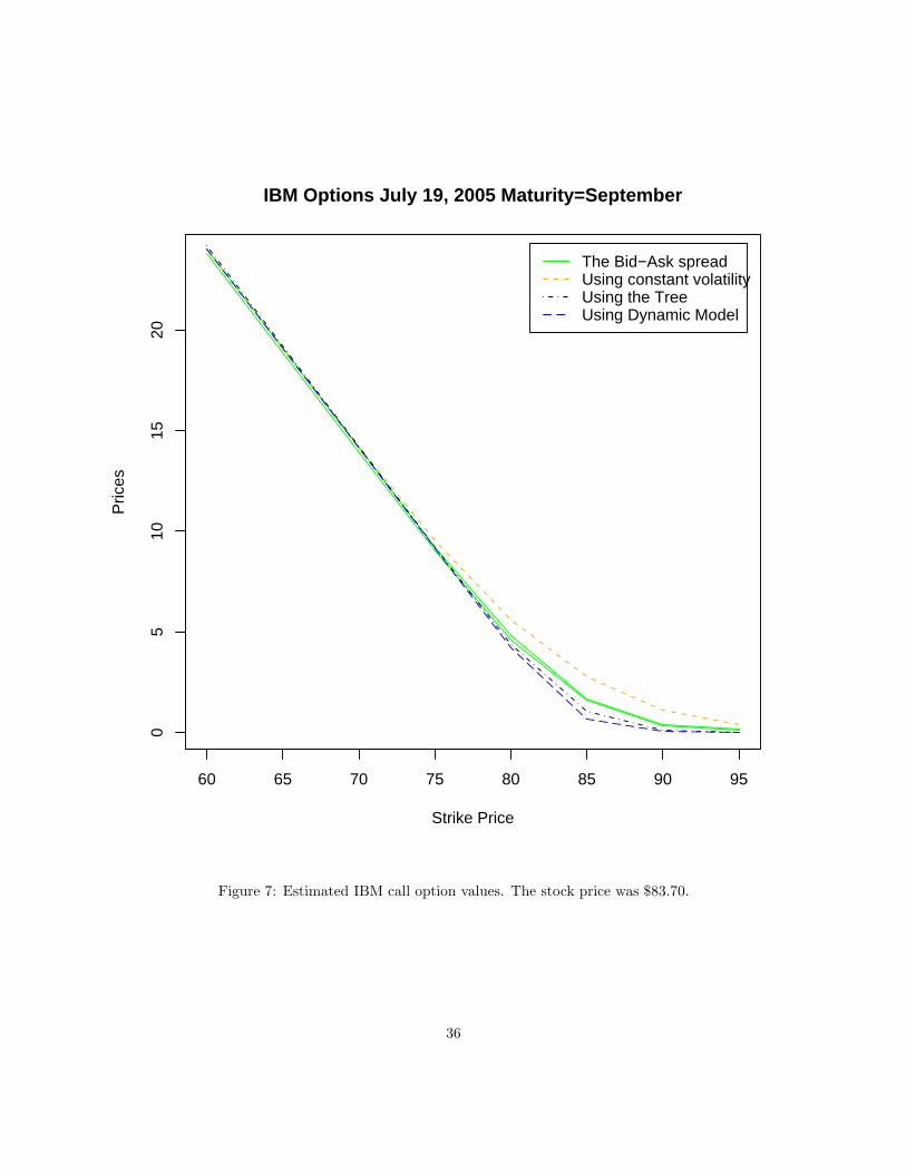


![Multi-asset derivatives: A Stochastic and Local Volatility ... · stochastic volatility and local volatility. One approach follows Gatheral’s [25] method of computing the local](https://static.documents.pub/doc/80x56/5f41b1a43e92b0386724b62b/multi-asset-derivatives-a-stochastic-and-local-volatility-stochastic-volatility.jpg)


