Motivation Expansion of the smile Asymptotics Heston model Bergomi model Numerical experiments Skew and skewness Conclusion Stochastic Volatility’s Orderly Smiles Julien Guyon Bloomberg L.P. Quant Research Fields Quantitative Finance Seminar Fields Institute for Research in Mathematical Sciences Toronto, February 6th, 2013 Joint work with Lorenzo Bergomi (SocGen) [email protected][email protected]Julien Guyon Bloomberg L.P. Stochastic Volatility’s Orderly Smiles
Transcript
Motivation Expansion of the smile Asymptotics Heston model Bergomi model Numerical experiments Skew and skewness Conclusion
Stochastic Volatility’s Orderly Smiles
Julien Guyon
Bloomberg L.P.Quant Research
Fields Quantitative Finance SeminarFields Institute for Research in Mathematical Sciences
Motivation Expansion of the smile Asymptotics Heston model Bergomi model Numerical experiments Skew and skewness Conclusion
Outline
Motivation
Expansion of the smile at order 2 in vol of vol
Short maturities and long maturities
First example: a family of Heston-like models
Second example: the Bergomi model with 2 factors on the variance curve
Numerical experiments
Rederiving the link between skew and skewness of log-returns
Conclusion
Julien Guyon Bloomberg L.P.
Stochastic Volatility’s Orderly Smiles
Motivation Expansion of the smile Asymptotics Heston model Bergomi model Numerical experiments Skew and skewness Conclusion
Motivation
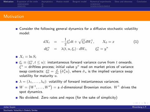
Consider the following general dynamics for a diffusive stochastic volatilitymodel:
dXt = −1
2ξttdt+
√ξttdW
1t , X0 = x (1)
dξut = λ(t, u, ξ·t) · dWt, ξu0 = yu
Xt = lnSt
ξ·t ≡ (ξut , t ≤ u): instantaneous forward variance curve from t onwards.ξu = driftless process; initial value yu read on market prices of varianceswap contracts: ξu0 = d
)= a d-dimensional Brownian motion. W 1 drives the
spot dynamics.
No dividend. Zero rates and repos (for the sake of simplicity)
Julien Guyon Bloomberg L.P.
Stochastic Volatility’s Orderly Smiles
Motivation Expansion of the smile Asymptotics Heston model Bergomi model Numerical experiments Skew and skewness Conclusion
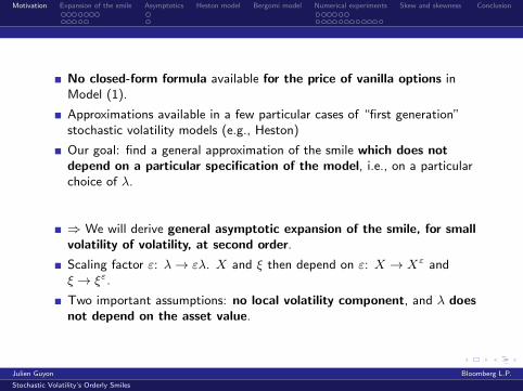
No closed-form formula available for the price of vanilla options inModel (1).
Approximations available in a few particular cases of “first generation”stochastic volatility models (e.g., Heston)
Our goal: find a general approximation of the smile which does notdepend on a particular specification of the model, i.e., on a particularchoice of λ.
⇒ We will derive general asymptotic expansion of the smile, for smallvolatility of volatility, at second order.
Scaling factor ε: λ→ ελ. X and ξ then depend on ε: X → Xε andξ → ξε.
Two important assumptions: no local volatility component, and λ doesnot depend on the asset value.
Julien Guyon Bloomberg L.P.
Stochastic Volatility’s Orderly Smiles
Motivation Expansion of the smile Asymptotics Heston model Bergomi model Numerical experiments Skew and skewness Conclusion
Smile produced by stochastic volatility models is generated by thecovariance of forward variances with themselves and spot.
Our goal: to pinpoint exactly which functionals of these covariancesdetermine the vanilla smile
Important to ensure, while varying ε, that implied volatilities of somespecific payoffs are unchanged, so that the overall volatility level is notaltered in the model.
In our framework, VS volatilities are unchanged as ε is varied.
Julien Guyon Bloomberg L.P.
Stochastic Volatility’s Orderly Smiles
Motivation Expansion of the smile Asymptotics Heston model Bergomi model Numerical experiments Skew and skewness Conclusion
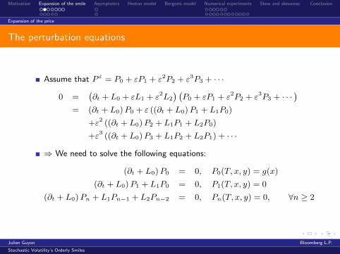
Expansion of the price
Expansion of the price of a vanilla option
Consider the vanilla option delivering g(XεT ) at time T .
Price P ε (t,Xεt , ξ·,εt ). We write P ε (t, x, y): the variable
y ≡ (yu, t ≤ u ≤ T ) is a curve.P ε solves the PDE (∂t + Lε)P ε = 0 with terminal conditionP ε(T, x, y) = g(x), where Lε = L0 + εL1 + ε2L2 with
L0 = −1
2yt∂x +
1
2yt∂2
x
L1 =
∫ T
t
du µ(t, u, y) ∂2xyu
L2 =1
2
∫ T
t
du
∫ T
t
du′ ν(t, u, u′, y) ∂2yuyu
′
µ(t, u, y) =√ytλ1(t, u, y) =
E [dXtdξut |ξt = y]
dt=
E[dStStdξut |ξt = y
]dt
ν(t, u, u′, y) =
d∑i=1
λi(t, u, y)λi(t, u′, y) =
E[dξut dξ
u′t |ξt = y
]dt
Julien Guyon Bloomberg L.P.
Stochastic Volatility’s Orderly Smiles
Motivation Expansion of the smile Asymptotics Heston model Bergomi model Numerical experiments Skew and skewness Conclusion
Motivation Expansion of the smile Asymptotics Heston model Bergomi model Numerical experiments Skew and skewness Conclusion
Expansion of the price
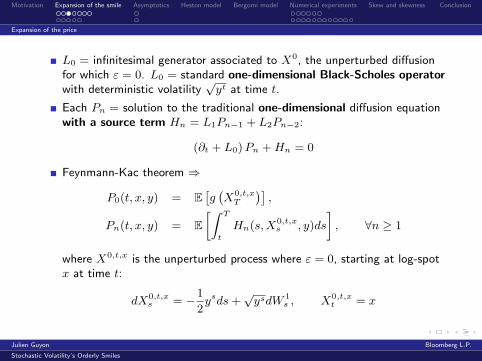
L0 = infinitesimal generator associated to X0, the unperturbed diffusionfor which ε = 0. L0 = standard one-dimensional Black-Scholes operatorwith deterministic volatility
√yt at time t.
Each Pn = solution to the traditional one-dimensional diffusion equationwith a source term Hn = L1Pn−1 + L2Pn−2:
(∂t + L0)Pn +Hn = 0
Feynmann-Kac theorem ⇒
P0(t, x, y) = E[g(X0,t,xT
)],
Pn(t, x, y) = E[∫ T
t
Hn(s,X0,t,xs , y)ds
], ∀n ≥ 1
where X0,t,x is the unperturbed process where ε = 0, starting at log-spotx at time t:
dX0,t,xs = −1
2ysds+
√ysdW 1
s , X0,t,xt = x
Julien Guyon Bloomberg L.P.
Stochastic Volatility’s Orderly Smiles
Motivation Expansion of the smile Asymptotics Heston model Bergomi model Numerical experiments Skew and skewness Conclusion
Expansion of the price
The price at order 0
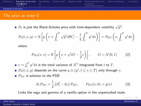
P0 is just the Black-Scholes price with time-dependent volatility√yt:
P0(t, x, y) = E[g
(x+
∫ T
t
√ysdW 1
s −1
2
∫ T
t
ysds
)]= PBS
(x,
∫ T
t
ysds
)where
PBS(x, v) = E[g
(x+√vG− 1
2v
)], G ∼ N (0, 1) (2)
v =∫ Ttysds is the total variance of X0 integrated from t to T .
P0(t, x, y) depends on the curve y ≡ (ys, t ≤ s ≤ T ) only through v.
PBS is solution to the PDE
∂vPBS =1
2
(∂2x − ∂x
)PBS , PBS(x, 0) = g(x) (3)
Links the vega and gamma of a vanilla option in the unperturbed state.
Julien Guyon Bloomberg L.P.
Stochastic Volatility’s Orderly Smiles
Motivation Expansion of the smile Asymptotics Heston model Bergomi model Numerical experiments Skew and skewness Conclusion
Expansion of the price
The price at order 0
An important observation:
Because L0 incorporates no local volatility, L0 and ∂x commute so(∂t + L0) ∂
pxP0 = ∂px (∂t + L0)P0 = 0.
⇒ ∂pxPBS(X0t ,∫ Ttysds
)≡ ∂pxP0(t,X
0t , y) is a martingale for all integer
p.
Equation (3) then shows that for all integers m,n,
∂mv ∂nxPBS
(X0t ,∫ Ttysds
)is a martingale.
This is crucial in the computations of P1 and P2.
Julien Guyon Bloomberg L.P.
Stochastic Volatility’s Orderly Smiles
Motivation Expansion of the smile Asymptotics Heston model Bergomi model Numerical experiments Skew and skewness Conclusion
Expansion of the price
The price at order 1
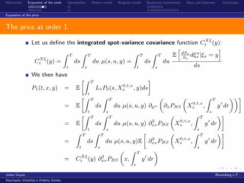
Let us define the integrated spot-variance covariance function CXξt (y):
CXξt (y) =
∫ T
t
ds
∫ T
s
du µ(s, u, y) =
∫ T
t
ds
∫ T
s
duE[dSsSsdξus |ξs = y
]ds
We then have
P1(t, x, y) = E[∫ T
t
L1P0(s,X0,t,xs , y)ds
]= E
[∫ T
t
ds
∫ T
s
du µ(s, u, y) ∂yu
(∂xPBS
(X0,t,xs ,
∫ T
s
yrdr
))]= E
[∫ T
t
ds
∫ T
s
du µ(s, u, y) ∂2xvPBS
(X0,t,xs ,
∫ T
s
yrdr
)]=
∫ T
t
ds
∫ T
s
du µ(s, u, y)E[∂2xvPBS
(X0,t,xs ,
∫ T
s
yrdr
)]= CXξt (y) ∂2
xvPBS
(x,
∫ T
t
yrdr
)Julien Guyon Bloomberg L.P.
Stochastic Volatility’s Orderly Smiles
Motivation Expansion of the smile Asymptotics Heston model Bergomi model Numerical experiments Skew and skewness Conclusion
Expansion of the price
The price at order 2
A similar result holds for the second order correction:
P2 = PL2P02 + PL1P1
2
PL2P02 (t, x, y) =
1
2Cξξt (y) ∂2
vPBS
(x,
∫ T
t
yrdr
)PL1P12 = PL1P1
2,0 + PL1P12,1
PL1P12,0 (t, x, y) =
1
2CXξt (y)2 ∂2
x∂2vPBS
(x,
∫ T
t
yrdr
)PL1P12,0 (t, x, y) = Cµt (y) ∂
2x∂vPBS
(x,
∫ T
t
yrdr
)
Cξξt (y) =
∫ T
t
ds
∫ T
s
du
∫ T
s
du′ ν(s, u, u′, y) =
∫ T
t
ds
∫ T
s
du
∫ T
s
du′E[dξus dξ
u′s |ξs = y
]ds
Cµt (y) =
∫ T
t
ds
∫ T
s
du µ(s, u, y) ∂yu(CXξs (y)
)Cξξt (y): integrated variance-variance covariance function
Julien Guyon Bloomberg L.P.
Stochastic Volatility’s Orderly Smiles
Motivation Expansion of the smile Asymptotics Heston model Bergomi model Numerical experiments Skew and skewness Conclusion
Expansion of the implied volatility
Expansion of the implied volatility
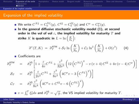
We write CXξ = CXξ0 (y), Cξξ = Cξξ0 (y) and Cµ = Cµ0 (y).
In the general diffusive stochastic volatility model (1), at secondorder in the vol of vol ε, the implied volatility for maturity T and
strike K is quadratic in L = ln(KS0
):
σ̂ε(T,K) = σ̂ATMT + ST ln
(K
S0
)+ CT ln2
(K
S0
)+O(ε3) (4)
Coefficients are
σ̂ATMT = σ̂VS
T
[1 +
ε
4vCXξ +
ε2
32v3
(12(CXξ
)2− v (v + 4)Cξξ + 4v (v − 4)Cµ
)]ST = σ̂VS
T
[ε
2v2CXξ +
ε2
8v3
(4Cµv − 3
(CXξ
)2)]CT = σ̂VS
Tε2
8v4
(4Cµv + Cξξv − 6
(CXξ
)2)v =
∫ T0ξs0ds and σ̂VS
T =√
vT
, the VS implied volatility for maturity T .
Julien Guyon Bloomberg L.P.
Stochastic Volatility’s Orderly Smiles
Motivation Expansion of the smile Asymptotics Heston model Bergomi model Numerical experiments Skew and skewness Conclusion
Expansion of the implied volatility
Comments
ATM implied volatility:
σ̂ATMT = σ̂VS
T
[1 +
ε
4vCXξ +
ε2
32v3
(12(CXξ
)2− v (v + 4)Cξξ + 4v (v − 4)Cµ
)]ATM implied volatility = variance swap volatility + spread. At first order,
spread = CXξ
4√vTε.
Typically, on the equity market, CXξ < 0: ATM implied volatility liesbelow the variance swap volatility.
When spot returns and forward variances are uncorrelated, CXξ = Cµ = 0so that
σ̂ATMT = σ̂VS
T
(1− ε2
32v3v (v + 4)Cξξ
)Because Cξξ ≥ 0, ATM implied volatility lies again below variance swapvolatility. The higher the volatility of variances, the smaller the ATMimplied volatility.
Julien Guyon Bloomberg L.P.
Stochastic Volatility’s Orderly Smiles
Motivation Expansion of the smile Asymptotics Heston model Bergomi model Numerical experiments Skew and skewness Conclusion
Expansion of the implied volatility
Comments (continued)
ATM skew: ST = σ̂VST
[ε
2v2CXξ + ε2
8v3
(4Cµv − 3
(CXξ
)2)]ATM skew ST is of order ε. It has the sign of CXξ. ST vanishes whenspot returns and forward variances are uncorrelated, even at second order.ATM skew is produced only by the spot-variance correlation.
Link ATM vol-VS vol-ATM skew:
σ̂ATMT = σ̂VS
T +
(σ̂VST
)2T
2ST
At first order in ε, ATM skew has same sign as the difference betweenATM implied volatility and variance swap volatility.
ATM convexity: CT = σ̂VST
ε2
8v4
(4Cµv + Cξξv − 6
(CXξ
)2)Curvature CT is of order ε2.
Not only does it involve variance/variance covariance: spot/variancecovariance (squared) contributes as well.
If spot and variances are uncorrelated, CT = Cξξ
8v5/2√Tε2 ≥ 0.
Julien Guyon Bloomberg L.P.
Stochastic Volatility’s Orderly Smiles
Motivation Expansion of the smile Asymptotics Heston model Bergomi model Numerical experiments Skew and skewness Conclusion
Expansion of the implied volatility
Another derivation which stays at the level of operators
Recall that the price P ε of the vanilla option is solution to(∂t + Lεt )P
ε = 0 with Lεt = L0,t + εL1,t + ε2L2,t, and terminal conditionP ε (T, x, y) = g(x).
Price can be expressed in terms of the semigroup (Uεst, 0 ≤ s ≤ t ≤ T )attached to the family of differential operators Lεt : P ε(t, ·) = UεtT g.
The semigroup is defined by
Uεst = limn→∞
(1− δtLεt0) (1− δtLεt1) · · ·
(1− δtLεtn−1
), δt =
t− sn
, ti = s+iδt
It satisfies Uεrt = UεrsUεst for 0 ≤ r ≤ s ≤ t ≤ T , hence the notation
: exp(∫ t
sLετdτ
):, where :: denotes time ordering.
We can directly expand Uεst in powers of ε. Usual time-dependentperturbation technique in quantum mechanics. U0
st is called the freepropagator.
Julien Guyon Bloomberg L.P.
Stochastic Volatility’s Orderly Smiles
Motivation Expansion of the smile Asymptotics Heston model Bergomi model Numerical experiments Skew and skewness Conclusion
Expansion of the implied volatility
Consider the general situation where a differential operator Lt is perturbedby another operator Ht: L
εt = Lt + εHt
From the definition of the semigroup, Uεst = U(0)st + εU
(1)st + ε2U
(2)st + · · ·
with
U(1)st =
∫ t
s
dτ U0sτHτU
0τt
U(2)st =
∫ t
s
dτ1
∫ t
τ1
dτ2 U0sτ1Hτ1U
0τ1τ2Ht2U
0τ2t
⇒ P ε = P0 + εP1 + ε2P2 + · · · , with
P1 =
∫ T
t
dτ U0tτL1,τU
0τT g
P2 =
∫ T
t
dτ U0tτL2,τU
0τT g +
∫ T
t
dτ1
∫ T
τ1
dτ2 U0tτ1L1,τ1U
0τ1τ2L1,τ2U
0τ2T g
We recover the expressions of P1 and P2.
Julien Guyon Bloomberg L.P.
Stochastic Volatility’s Orderly Smiles
Motivation Expansion of the smile Asymptotics Heston model Bergomi model Numerical experiments Skew and skewness Conclusion
Short maturity
Short maturity
Assume dξtt = · · · dt+ ε(ξtt)ϕdBt
Let ρSV be the correlation between St and instantaneous variance Vt = ξtt
⇒ Short-term ATM skew does not depend on short-term ATM vol iffϕ = 1 (observed in equity markets)
⇒ Short-term ATM convexity does not depend on short-term ATM vol iffϕ = 5
4. And (∀ρSV , C0 ≥ 0)⇐⇒ ϕ ≥ 5
4
Julien Guyon Bloomberg L.P.
Stochastic Volatility’s Orderly Smiles
Motivation Expansion of the smile Asymptotics Heston model Bergomi model Numerical experiments Skew and skewness Conclusion
Long-term asymptotics of implied volatility
Long-term asymptotics of implied volatility
Assume the term-structure of variance swaps volatilities is flat: ξt0 ≡ ξ.
Assume that for large u− t, µ(t, u, y) ∝ (u− t)−α, α > 0.Then at higher order in ε, for long maturities,
ST ∝ T−α if α < 1
ST ∝ T−1 if α > 1
α is exactly a signature of the long-time decay of the spot/variancecovariance function.
Assume that for large u− t and u′ − t,ν(t, u, u′, y) ∝ (u− t)−β(u′ − t)−β , β > 0.Also assume that spots and volatilities are uncorrelated (µ ≡ 0). Then athigher order in ε, for long maturities,
CT ∝ T−2β if β < 1
CT ∝ T−2 if β > 1
Exponential decay ↔ β > 1.
Julien Guyon Bloomberg L.P.
Stochastic Volatility’s Orderly Smiles
Motivation Expansion of the smile Asymptotics Heston model Bergomi model Numerical experiments Skew and skewness Conclusion
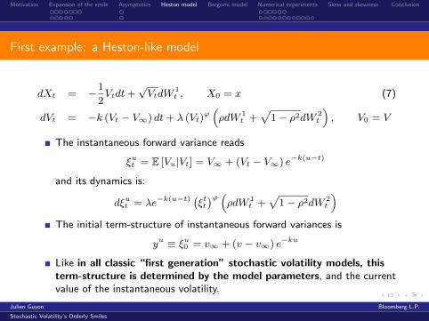
First example: a Heston-like model
dXt = −1
2Vtdt+
√VtdW
1t , X0 = x (7)
dVt = −k (Vt − V∞) dt+ λ (Vt)ϕ(ρdW 1
t +√
1− ρ2dW 2t
), V0 = V
The instantaneous forward variance reads
ξut = E [Vu|Vt] = V∞ + (Vt − V∞) e−k(u−t)
and its dynamics is:
dξut = λe−k(u−t)(ξtt)ϕ (
ρdW 1t +
√1− ρ2dW 2
t
)The initial term-structure of instantaneous forward variances is
yu ≡ ξu0 = v∞ + (v − v∞) e−ku
Like in all classic “first generation” stochastic volatility models, thisterm-structure is determined by the model parameters, and the currentvalue of the instantaneous volatility.
Julien Guyon Bloomberg L.P.
Stochastic Volatility’s Orderly Smiles
Motivation Expansion of the smile Asymptotics Heston model Bergomi model Numerical experiments Skew and skewness Conclusion
The volatility λ(t, u, y) of instantaneous forward variances depends on theinstantaneous forward variance curve y = (ys, t ≤ s ≤ T ) only through theinstantaneous spot variance yt:
λ1(t, u, y) = ρ(yt)ϕe−k(u−t)
λ2(t, u, y) =√
1− ρ2(yt)ϕe−k(u−t)
As a consequence,
CXξ =ρ
k
∫ T
0
ds (ys)ϕ+12
(1− e−k(T−s)
)Cξξ =
2∑i=1
∫ T
0
ds
(∫ T
s
duλi(s, u, y)
)2
=1
k2
∫ T
0
ds (ys)2ϕ(1− e−k(T−s)
)2Cµ =
(ϕ+
1
2
)ρ2
k
∫ T
0
ds (ys)ϕ+12
∫ T
s
du (yu)ϕ−12 e−k(u−s)
(1− e−k(T−u)
)This coincides with Equations (3.7) to (3.10) in Lewis [7], whereJ(1) = CXξ, J(3) = 1
2Cξξ, and J(4) = Cµ
Julien Guyon Bloomberg L.P.
Stochastic Volatility’s Orderly Smiles
Motivation Expansion of the smile Asymptotics Heston model Bergomi model Numerical experiments Skew and skewness Conclusion
Motivation Expansion of the smile Asymptotics Heston model Bergomi model Numerical experiments Skew and skewness Conclusion
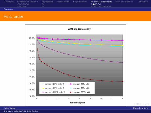
First order
First order ��������������� ����� ���������� �������������������������������������������������������������������������� ��� ���� ���� ���� ������ �!����" #$���� %��$������" ������ ���������� ���������������������������������������������������Julien Guyon Bloomberg L.P.
Stochastic Volatility’s Orderly Smiles
Motivation Expansion of the smile Asymptotics Heston model Bergomi model Numerical experiments Skew and skewness Conclusion
First order
First order
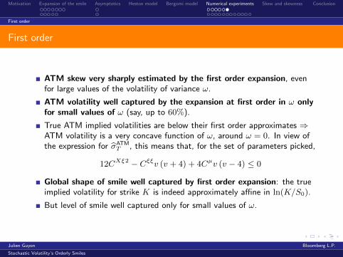
ATM skew very sharply estimated by the first order expansion, evenfor large values of the volatility of variance ω.
ATM volatility well captured by the expansion at first order in ω onlyfor small values of ω (say, up to 60%).
True ATM implied volatilities are below their first order approximates ⇒ATM volatility is a very concave function of ω, around ω = 0. In view ofthe expression for σ̂ATM
T , this means that, for the set of parameters picked,
12CXξ2 − Cξξv (v + 4) + 4Cµv (v − 4) ≤ 0
Global shape of smile well captured by first order expansion: the trueimplied volatility for strike K is indeed approximately affine in ln(K/S0).
But level of smile well captured only for small values of ω.
Julien Guyon Bloomberg L.P.
Stochastic Volatility’s Orderly Smiles
Motivation Expansion of the smile Asymptotics Heston model Bergomi model Numerical experiments Skew and skewness Conclusion
Second order
Second order
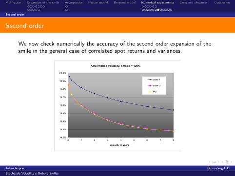
We first consider the situation when spot returns and forward variances areuncorrelated. In this case, the ATM skew vanishes, and so does its expansion atsecond order in ω. We pick
Motivation Expansion of the smile Asymptotics Heston model Bergomi model Numerical experiments Skew and skewness Conclusion
Second order
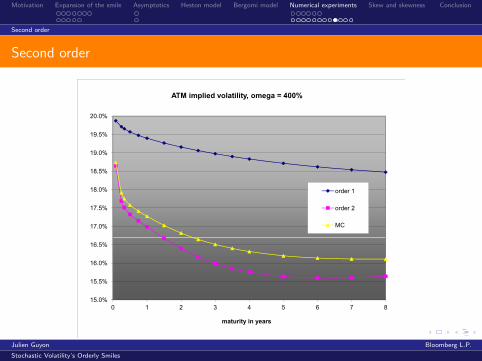
Second order
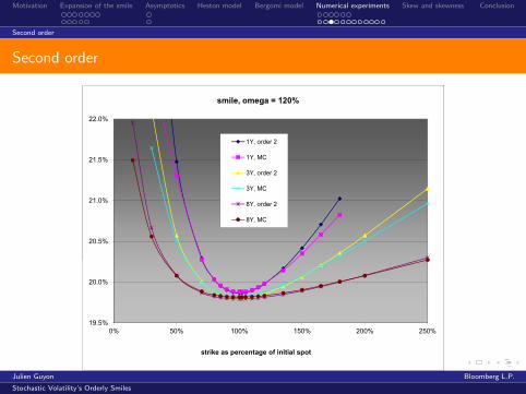
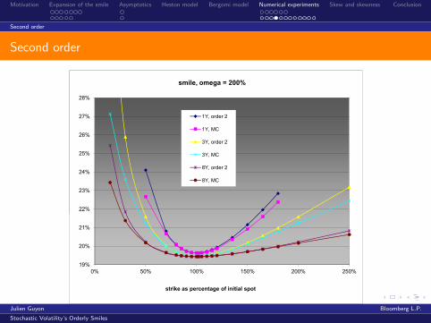
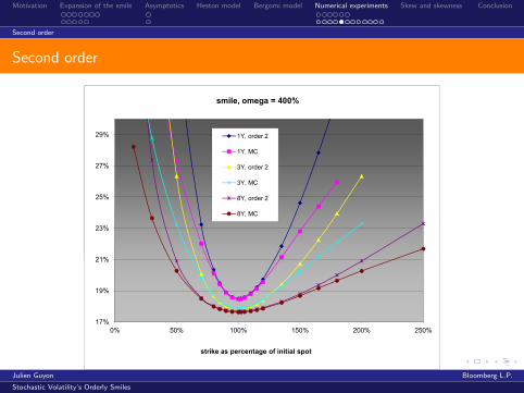
ATM implied volatility very sharply estimated by the second orderexpansion, even up to ω = 400% and to long maturities. For T = 15years, estimate is less than 15 bps above true ATM volatility.
Looking at the whole smile: second order expansion of the impliedvolatility is excellent around the money, but becomes too large for strikesfar from the money.
Not surprising: No arbitrage ⇒ for very small and very large strikes,σ̂(T,K)2 grows at most linearly with ln(K/S0) (see Lee [6]), whereassecond order estimate for σ̂(T,K)2 grows like ln4(K/S0), see (4).Remainder O(ω3) = R(ω, T,K) is large for large K, for finite ω.
Nevertheless, even for ω = 400%, a maturity of 8 years and anout-the-money strike of 250%, the error is only 1.5 point of volatility.
Julien Guyon Bloomberg L.P.
Stochastic Volatility’s Orderly Smiles
Motivation Expansion of the smile Asymptotics Heston model Bergomi model Numerical experiments Skew and skewness Conclusion
Second order
Second order
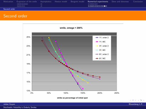
We now check numerically the accuracy of the second order expansion of thesmile in the general case of correlated spot returns and variances.���������������������������� �� ������� ����������� ����� � ���� !"#!$� !"#!$�%&��������'����(� � � ' ( � � � ����)*��� �+ ���*,
Julien Guyon Bloomberg L.P.
Stochastic Volatility’s Orderly Smiles
Motivation Expansion of the smile Asymptotics Heston model Bergomi model Numerical experiments Skew and skewness Conclusion
Motivation Expansion of the smile Asymptotics Heston model Bergomi model Numerical experiments Skew and skewness Conclusion
Remember ST = CXξ
2v3/2√Tε+O
(ε2)
Let us now compute the skewness sT of log-returns:
sT =E[X 3T
]E [X 2
T ]3/2
, XT = XT − E [XT ] =
∫ T
0
√ξt,εt dW 1
t
We have E[X 2T
]=∫ T0ξt0dt+O(ε) and
E[X 3T
]= 3εCXξ +O
(ε2)
At first order in the vol of vol, the skewness of (the distribution of)ln (ST /S0) is thus
sT =3εCXξ(∫ T
0ξt0dt
)3/2The ATM skew ST simply reads
ST =sT
6√T
+O(ε2)
Julien Guyon Bloomberg L.P.
Stochastic Volatility’s Orderly Smiles
Motivation Expansion of the smile Asymptotics Heston model Bergomi model Numerical experiments Skew and skewness Conclusion
Conclusion
We provide an expansion at order two in volatility-of-volatility for generalstochastic volatility models based on a forward variance formulation.
VS volatilities for all maturities are unchanged as ε is varied.
At order two in ε, the smile is exactly quadratic in log-moneyness anddepends on only three model-dependent dimensionless quantities:
CXξ, the integrated spot/variance covariance function,Cξξ, the integrated variance/variance covariance function,Cµ, which, like Cxξ, depends only on instantaneous spot/variancecovariances.
We shed light on the significance of CXξ by establishing a simple linkbetween the ATM skew and the skewness of lnST .
Julien Guyon Bloomberg L.P.
Stochastic Volatility’s Orderly Smiles
Motivation Expansion of the smile Asymptotics Heston model Bergomi model Numerical experiments Skew and skewness Conclusion
From our general expression we derive the short-maturity limits of ATMvolatility, skew, curvature: we give structural dependencies of the ATMskew and curvature on ATM volatility.
We also link the long-term decay of the ATM skew and curvature to thedecay of spot/variance and variance/variance covariance functions.
Numerical experiments in the case of a two-factor version of the Bergomimodel show good agreement of the order one expression for the ATMskew, and of the order two expression for the ATM volatility, for values ofthe volatility of short-dated variance (around 400%) that are typical ofimplied levels of equity indices.
Julien Guyon Bloomberg L.P.
Stochastic Volatility’s Orderly Smiles
Motivation Expansion of the smile Asymptotics Heston model Bergomi model Numerical experiments Skew and skewness Conclusion
Benhamou E., Gobet E. and Miri M., Smart expansion and fast calibrationfor jump diffusion, Finance and Stochastics, Vol.13(4), pages 563-589,2009.
Bergomi L. and Guyon J., Stochastic Volatility’s Orderly Smiles, RiskMagazine, pages 60-66, May 2012.