1

Stochasticity and Uncertainty

Experimentally Investigating Preference (In)Consistency in Two-Stage Decision

Problems

Abstract

We report on an experimental investigation into four prominent theoretical models of

two-stage decision-making, in which the decision maker (DM) makes a choice of a

menu in the first stage and then makes a choice from the chosen menu in the second

stage. Each of these models axiomatically derives a preference functional dictating

choice of the menu; some of them explicitly also specify choice at the from stage. Our

experiment uses lotteries as the final objects of choice, and we describe preferences

by the degree of risk aversion. We examine the goodness-of-fit of the four models in

explaining the choice of the menu, and the goodness-of-fit in explaining the choice

from the menu for the two of the four models who explicitly model the second-stage

choice. Our results indicate that our subjects’ behaviour is best explained by a random

indulgence model.

Keywords: two-stage decision problems, choosing a menu, choosing from the menu,

commitment, temptation, self-control, changing preferences

Lihui Lin and John Hey,

Department of Economics, University of York, Heslington, York, YO10 5DD.

Lin: ll1654@york.ac.uk; Hey: John.hey@york.ac.uk

Acknowledgements: We are grateful to the Leverhulme Trust for generously funding

this research with Leverhulme Emeritus Grant EM-2019-026/7

2

1. Introduction

A common decision scenario in life is that of making a menu choice, and then a choice

from the chosen menu, such as choosing a restaurant and choosing food from this

restaurant; choosing an insurance provider and choosing one scheme from this

provider; and so on. A menu can be interpreted either literally or as an action

concerning an opportunity set that will affect subsequent opportunities. In this context,

dynamic (in-)consistency across the two stages will determine what decision makers

do.

This two-stage decision problem has recently been widely addressed in economic and

decision theory research. One of the most popular classes of models is that of Gul and

Pesendorfer (2001) (henceforth GP). This is termed a “self-control and temptation

model” which incorporates ex-ante preference, commitment demand and self-control

to resist temptation, to account for any dynamic inconsistency. GP model two types of

decision-makers – henceforth DMs – (namely, ‘self-control’ and ‘temptation

overwhelming’) .The widely discussed GP’s self-control model characterises a DM who

experiences temptation at the moment of choice from a menu and who anticipates

this in the first stage, where she1 selects which menu to face. In this first stage, the DM

has a particular perspective on what she should choose from menus, embodied in a

“normative preference”. The DM understands that her choice from menus will not

necessarily respect the normative preference, but rather will seek to balance her

normative preference with the cost of resisting temptation or giving in to the

temptation. Accordingly, the self-control DM may dislike a larger choice set since it

may include tempting choices, which are not desirable from the earlier perspective.

1 For ‘she’ read ‘he or she’ throughout and similarly for ‘her’, mutatis mutandis.

3

There are other models following this line but adopting different perspectives. GP

suggests that not only the actual utility will matter, but that the existence of tempting

problems will lower utility. In this information-explosion era, available choices are

many, thus we usually will be exposed to many problems that may conflict with our

long-term normative preferences. A generalization of GP, Stovall (2010), (henceforth

Stovall), considers a situation where DMs are tempted by multiple temptations, and

hence incur higher costs to resist more temptations when temptation preferences are

uncertain. Another generalization of GP in terms of uncertainty is Chatterjee and

Krishna (2000) (henceforth CK). While Stovall and GP both include a cost of self-control

when the DM excludes possible temptations. CK addresses a cost of from the risk of

succumbing, that is, from ‘random indulgence’ rather than costly self-control: the DM

implements a dual-self-evaluation – the long-term normative preference and the

temptation driven preference – incorporating the fact that the individual considers the

possibilities of both selves.

Some argue that ignoring the future choice when taking the initial choice is not

necessarily optimal when new information regarding preferences or other variables is

expected to arrive in the future (Amador and Werning, 2005), since future preferences

may be uncertain in many cases. The literature interprets this anticipation of uncertain

future tastes as a preference for flexibility (Kreps, 1979). In this information-overload

era, the existence of many possible choices may distract attention and consequently

increase preference uncertainty. Flexibility models suggest that a larger set with a

range of possible future preferences will be preferred; this conclusion is opposite to

that of GP. For example, one of the flexibility models in the same two-stage decision-

making context is Ahn and Sarver (2013) (henceforth AS)’s model which incorporates

4

preference flexibility and random utility theory. They model a DM who is uncertain

about her future preferences and anticipates the probabilities of each choice she will

make in the future and how much utility these choices will provide. The DM

correspondingly evaluates menus in the first stage according to these correct

predictions. In the second stage, one subjective state will be realised, and DM will

maximise the utility given this state. The key feature of self-control (as distinct from

flexibility) is the desire to keep commitment and eliminate possible temptations. The

price of flexibility is the cost of thinking (Ortoleva, 2013), such as keeping concentrated

or rational in a distracting context; while avoiding the existence of temptation could

reduce the distraction and temptation even though the cost of self-control and

opportunity should be incorporated.

Given the difference between these various models, several questions arise. The main

purpose of this paper is to report on an experimental test of the above-mentioned

models and understand how ex-ante preference translates into the choice of a menu

and the subsequent choice from the chosen menu in a reasonably general context.

Investigating the choice patterns in this context and assessing the quantitative strength

of commitment, temptation and flexibility preference across choices offers insights

into how decision-makers view and consider temptation, and thus how policy makers

may eliminate or manipulate the temptation. In this information-explosion era,

available choices are many, and marketeers use elaborate marketing schemes, such as

nudging, anchoring, discount and bundling, to tempt consumers. In most daily

scenarios, the existence of other choices is a source of temptation, which will distract

and may overwhelm attention and willpower; subsequently the compulsive desire to

engage in short-term urges for enjoyment conflicts with long-term goals. Normally,

5

some unexpected possibilities might look good for some reasons in particular contexts.

Students who want to study on their own, if there are mobile calls or distracting

sounds, find it easy to change their choices. People who want to have saving plans can

easily change their decision if they go to a mall with large discounts. An investor who

has suffered multiple investment failures may decide to make a more risk-averse

portfolio ̶ however, she may be persuaded to choose a particularly high-return gamble

when the investment manager offers such options. Thus, as we will discuss later when

we describe our experimental design, we introduce temptation by inserting both very

safe, and very risky lotteries, into the menu to distract choices. Thus, by “temptation”

and “self-control” in our case, we applied Dekel, et al (2009)’s definition: “we mean

that the agent has some current view of what actions she would like to choose, but

knows that at the time these choices are to be made, she will be pulled by conflicting

desires.” We refer to temptations as problems extremely different from ex-ante and

planned-to-implement preferences. However, we should note that the motive of self-

control is not our main interest. Most decisions of our daily life do not always involve

right-and-wrong questions, but the conflict between long-term desire and current

tempting desires may lead to negative feelings. We focus on measuring how actual

choice deviates from ex-ante preference by the intervention of temptation. Ex-ante

preference and commitment are valuable for ex-ante surveys, such as polls, consumer

preference surveys, saving and consumption plans, which are considered by policy

makers and business decision makers. Furthermore, the choice of menu is a set of

chosen opportunities for the future final consumption. It is meaningful for future

market prediction.

6

Despite the obvious importance of the topic, as illustrated above, it is difficult for

empirical research to investigate ex-ante commitment preference, temptation

preference and flexibility preference in one context. This has been partly done by

Toussaert (2018) who designed an experiment to test GP focusing on the self-control

type identification. Her experiment implements the temptation by offering additional

earnings to read a sensational story during a tedious attention task for which subjects

received payment. In our paper, we report on a more general experiment which tests

and compares these four models. Our experiment generalises the environment in

order to carry out parametric estimation and an assessment of the relative explanatory

abilities of the different models.

We follow the theoretical models’ use of menus as sets of lotteries, and lotteries will

be used to infer risk preferences. Our experiment involves a three-step procedure to

infer the commitment preference, temptation preference and flexibility preference.

First, we elicit the subjects’ ex-ante preference (singleton evaluations of lotteries)

using (our slight modification of) Holt-and-Laury’s price list method and hence infer

the ranking of singleton menus. Second, subjects were asked to choose one menu from

a set of menus; and third, choose an option from the chosen menu. Importantly, we

give different subjects different menus according to their ex-ante risk preferences; this

embodies the idea of a personalised offering based on an ex-ante market survey (as

current online shopping websites do). We implement the temptation by offering

certainty choices, very low-risk choices (a high probability of getting a low payoff) and

very high-risk choices (a low probability of getting a high payoff). In addition, to

implement the flexibility, the size of the menus varies. Menusets are designed carefully

to promote the tradeoff between the cost of self-control and the opportunity cost:

details are given in the experimental design section.

7

We should note that there is a large literature in psychology and decision science,

which has discussed self-control, commitment and flexibility demand, willpower and

temptation. Toussaert (2018) and Dean and McNeill (2015) experimentally explore the

GP and AS models and study commitment and flexibility, but our design is different.

We generalise the temptation trying to reflect our most daily decision scenarios – not

strictly right or wrong/good or bad decisions. To our knowledge, we are the first to

conduct parametric estimation and qualitatively measure the different preferences,

that is, ex-ante preference, and temptation (ex post) preference. Crucially, the

importance of menu choice research is that the chosen menu determines the

subsequent opportunity set and hence the final decision or consumption. While most

research in this field focus on the choice of menu stage, we go one step further by

examining also the choice from the chosen menu to test the predictive power of

models and behavior consistency. Believing that economics is all about predicting,

rather than just explaining, we compare four of our models by seeing how good they

are at predicting choice from the menu, that is, final consumption. However, with our

data, we only can test the predictive power of the from stage in GP and CK models (this

is because we cannot observe the realized preference in each decision or have enough

observations to fit the from stage of the Stovall and AS models). We elaborate on this

point in section 2.

This paper is organised as follows. Section 2 introduces the models. Section 3

compares and contrasts them, using a motivating example. Section 4 describes the

experimental design and section 5 the econometric specification. Section 6 discusses

and interprets the results. Section 7 concludes with a summary of the results, a

discussion of findings and implications

8

2. Models and a motivating example

The motivation for the model comparisons is based on the distinctions between the

different two-stage decision making models. This section discusses the models that we

investigate, and describes how flexibility preference, self-control and temptation

influence the decision making over menus and the corresponding implied choice from

the chosen menu. While Stovall and CK only address the choice of menu stage, we

extend these models into two stage models induced from the of stage. We also justify

why we have difficulty in predicting and estimating the from stage of AS and Stovall

with our experimental data.

We pay particular attention to preference functionals in terms of ex-ante preference u

(that is the preference over singleton lotteries), the menu preference U, and the ex-

post preference v (that is, the temptation preference)2. We present the behavioural

representations and intuitions. We do not explore the theorems and axioms, leaving

that to the original papers.

2.1 Self-control and temptation in GP 2001

This paper studies a two- stage model where ex-ante inferior choice may tempt the

decision-maker in the second stage. Individuals have preferences over sets of

alternatives that represent second stage choices. Their axioms yield a representation

that identifies the individual’s commitment ranking over singletons (that is, ex-ante

preference u), temptation ranking (that is, ex post temptation preference v), and the

2 Both u and v are von Neumann-Morgenstern utility functions over lotteries.

9

cost of self-control. An agent has self-control (self-control subject) if she resists

temptation and chooses an option with a higher ex-ante utility. The paper also models

another type of agent (temptation overwhelming subject) who is overwhelmed by the

temptations and gives in to them.

The preference functional for the choice of menu in GP is given by

For a self-control DM (henceforth GP type 1)

( ) max ( ) ( ) max ( )U A u x v x v y where ,x y A (1)

For a temptation-overwhelmed DM (henceforth GP type 2)

( ) max ( ) subject to ( ) ( ) for all U A u x v x v y y A , where ,x y A (2)

Here A is a menu of lotteries and ,x y A . For a self-control DM, GP interprets

max[ ( ) ( )]v y v x as the cost of self-control. Since the cost is always positive, the

existence of temptation in the menu will decrease the utility of the menu. Thus, the

self-control DM may anticipate the temptation and will tend to avoid the temptations

in the menu. This suggests that a smaller menu size without temptation will always be

preferred. At the choice from menu stage, they suggest an optimal compromise

between the utility of commitment preference u and the temptation preference v by

maximizing u+v. However, self-control is a limited mental resource. When the cost of

self-control is too high, the DM might end up with giving into the temptation. So, for

the temptation-overwhelmed DM, she values more the temptation and thus

maximises the temptation utility v first then evaluates these choices based on the

commitment preference u. After choosing the menu, a temptation-overwhelmed DM

10

gives in to the temptation by choosing the lottery with the maximum temptation utility

from the chosen menu.

2.2 Multiple temptations in Stovall

This model generalises GP by considering a decision maker who is tempted by multiple

normatively (ex-ante) worst alternatives. At the same time, she would want to expand

her choice set by including normatively superior alternatives. As Stovall argues, in the

choice of menu stage the DM is not tempted by any alternatives but just predicts the

possible state at the time of choosing from the menu. Put simply, the DM anticipates

the future possible temptations and maximises the maximum expected utility her

present self can obtain by choosing among the realised future self’s most preferred

lotteries in the menu. A DM wants to choose a menu of opportunity sets for a future

period of time so as to maximise the utility of the menu as evaluated as the present

moment. However, she is uncertain what will tempt her in the future, so all the

possible temptations will be considered. The model suggests that the agent is

uncertain which of these temptations will affect her.

The preference from menu functional for Stovall is

1

( ) {max ( ) ( ) max ( )}s

s s ss

U A q u x v x v y

where ,x y A (3)

Here s S is the subjective state. There are multiple temptations and sq is the

probability of being tempted by temptation ( )sv y . In state s, ( )sv y is the temptation

that affects the agent. Similar to GP, the DM compromises between the normative

preference and temptation preference and chooses the alternative that maximises

11

su v conditional on the subjective state s . Meanwhile, the DM experiences the

disutility of self-control, which is the foregone utility from the most tempting

alternative. The model suggests that the DM is uncertain which of the temptations will

affect her. This model implies that adding a normatively superior option into any menu

will increase the utility of the menu while adding a temptation into the menu will make

the menu less desirable. The DM evaluates the menu by trading off the normatively

superior option and anticipating possible temptations. This model shares the same

spirit of GP’s self-control. A menu with more temptations will be avoided by exerting

self-control; thus, a smaller size of menu will be preferred.

Stovall does not model the choice from the menu stage3. His model is a generalisation

of GP (called ‘random GP’) and is a special case of Dekel et al (2001)’s model. According

to the justification of Dekel And Lipman (2012), a random GP representation

generalizes the notion of a GP representation in a fashion exactly analogous to the GP

with the maximiser of u v from the menu, given the probability sq ; specifically, the

u is fixed, but there is an anticipated probability measure over the “temptations” ,

while at the final stage, the preference uncertainty will be resolved, that is, one state

will be realized.

2.3 Stochastic Temptation in CK

3 He writes (page 350): “It is understood, though unmodeled, that she will later choose an alternative from the

menu she chooses now.”

12

GP and Stovall are grounded on the conflict between ex-ante normative preference

and ex-post temptation preference. There is another perspective to model the conflict

and the consistency between preferences. CK models them by a dual self with a

stochastic story. Differing from using strong self-control to avoid the existence of

temptation, DMs are modelled as considering the possibility of being tempted in the

future rather than excluding all possibilities with cost of self-control at the first stage.

This model interprets temptation as a systemic mistake in which the second-stage

choice could be interpreted as being made by an “alter ego” who appears randomly:

DMs at the first stage consider the probabilities to be tempted at the second stage.

The choice of menu preference functional of CK is

( )( ) (1 )max ( ) max ( ) where ( ) is the set of maximisers in vx A y B A vU A q u x q u y B A v A

(4)

where q is the probability of being tempted. CK refer to their model as a dual-self

model, where u is the utility function of the long run self and v is the utility function

of the other self. When making the choice of menu, the DM believes she has q

probability that the other self will dominate at the choice from the menu stage; that

is, giving into the temptation. Following the spirit of self-control, the representation

could be interpreted as an internal battle for self-control with the alter ego where q is

the probability to lose self-control.

As noted above, the choice from the menu stage is unmodeled in CK. However, it

seems reasonable to follow the decision rules implicit in CK’s discussion: “a decision

maker who satisfies our axioms behaves as if there is a probability of her being

tempted when a choice has to be made from a menu, which is represented as the

choice being made by an alter ego. It should be emphasised that the alter ego (and his

13

utility function v) is subjective, as is the probability, q of getting tempted.” Thus, two

selves, that is, self-control or giving into temptation, one will stochastically dominate

at the choice from menu stage given the probability q, (q is the probability to choose

the maximum v, and 1-q the probability to choose the maximum u from the chosen

menu).

2.4 Preference Flexibility and Random Choice in AS

In marked contrast with the self-control and temptation stories, AS considers a story

where ex-ante preference (commitment in GP) does not play a role in the first stage

choice due to the preference uncertainty. Thus, there are no conflicts between the

normative preference and the temptation preference. They suggest a two-stage model

incorporating the preference flexibility of DLR and the random choice of Gul and

Pesendorfer (2006). They model a DM who is uncertain about her future preferences

and anticipates the probabilities of each choice she will make in future and how much

utility these choices will provide. The DM evaluates menus in the first stage according

to these correct predictions4. In the second stage, one subjective state will be realised

(which is a random draw from the belief distribution at the first stage), and the DM will

maximise utility given this state.

The preference of menu functional for AS is

( ) ( )max ( )sU A q s v x where x A (5)

4 Their model proposed the condition of correct belief on future preference contingency. But it does not guarantee the belief will be necessarily correct in reality. We also tested this in our experiment.

14

Where s S is the subjective state and the 'q s are the probabilities of anticipated

future preferences. So, the utility of a menu A is equal to the expected utility of the

best option in A, with expectations taken over the different possible utility functions

indexed by the state S, which we refer to as the belief about the preferences at the

second stage. This model suggests that the DM will prefer flexible menus, which offer

many possible future choices. A simple case is that we might be unsure whether we

would like to have cheesecake or scone before we actually go to the restaurant. Thus,

simply choosing the restaurant that offer everything will be easier way. As for the

choice from the menu, AS suggests that the DM maximises the utility given the realised

state. So, we will know which we actually want to choose when we go to the restaurant

and make the final decision.

3. Connections and Differences between the Models

The four models we are investigating describe behaviour in our two-stage setting from

different perspectives. For example, you want to buy a new computer. You also have a

saving plan to consider. Your ex-ante normative preference are the cheaper the better.

However, once you start searching online you may be persuaded otherwise by

discounted offers, PC reviews or overall popularity. In this scenario, we may consider

3 options:

A) a website that only offers cheap computers {a, b};

B) a site that offers several popular but more expensive brands {c, d};

C) Offers all of the above {a, b, c, d}.

15

Suppose your preferences are as follows: ( ) ( ) ( ) ( )u a u b u c u d and

( ) ( ) ( ) ( )v a v b v c v d .

A costly self-control GP DM will avoid the existence of temptation by choosing the

smallest size of menu, that is, the website A with only cheap computers because she

wants to avoid the potential risk to lose control and change her original purchase plan.

A temptation-overwhelmed GP, thinks that she may give in to the temptation ̶

evaluating the menus by the ex-ante utility of the most tempting. Thus, menu A is

evaluated as u(b); menu B is evaluated as u(d) and menu C as u(d). Thus, website A is

preferred. If she is uncertain about the temptation, she would be a Stovall DM who

considers the possibilities to give in to each temptation and avoids all possible

temptations, that is the possibilities to be tempted by d, c and b. Clearly, the website

A will be still preferred. Similarly, a CK DM also considers the possibilities to be tempted,

but only considers the most tempting one, that is b in menu A, d in the menu B and d

in the menu C (since she evaluates succumbing to temptation by the ex-ante

preference); thus a CK subject also will choose website A. We see that GP, Stovall and

CK suggest the same choice of menu.

However, an AS DM enjoys the larger choice set in the presence of uncertainty and

forgets her ex-ante money-saving plan and browses the websites at random. The

flexibility will provide an easier way to choose the menu where opportunity costs do

not exist. All the possibilities will be taken into consideration. The menu that contains

more possibilities will be preferred, that is website C.

In summary, each model implies a particular preference functional. Some of them lead

to the same choice of menu, while different final decisions from the menu. We can see

that they also have connections. GP and Stovall postulate the motives of self-control

16

and disutility of temptation. Stovall is a generalisation of GP. Stovall and AS address

uncertainty and flexibility. However, flexibility and possibility play different roles in

Stovall and AS. CK is a generalisation of GP Type 2. GP, Stovall and CK can be

interpreted as multiple-self stories. In these models, present-biased subjects may

demand the commitment devices to constrain the choices of the future selves if they

expect to succumb to temptation while addressing the conflicts between the tempted

self and the ex-ante long term self. While AS does address this, AS does not suggest

excluding possibilities as do GP and Stovall. On the other hand, CK could be a special

case of AS, when ex-ante preference is the temptation preference and there is only

one possibility.

Our experiment is designed to investigate these differences and connections.

3.1 Whether the strength of ex-ante preference or preference flexibility is prevalent

in reality

GP, Stovall and CK are dependent on the conflict between ex-ante normative

preference and ex-post temptation preference(s). The DM has to exert self-control to

resist this conflict. In contrast, AS addresses a preference for flexibility where ex-ante

preference do not impinge on subsequent decisions. Consider three menus {a}, {b},

{a,b} with preferences u(a)>u(b) and v(a)<v(b). Then GP, CK and Stovall would imply

{a} > {a, b} > {b}. However, AS would suggest {a,b} will be preferred over {a} and {b}.

This is what is generally referred to as ‘Preference for Flexibility’, and it results in

preference for a larger menu set. It is this property, which distinguishes the preference

uncertainty models from models of temptation and self-control in which smaller

choice sets may be preferred to avoid exposure to tempting problems.

17

3.2 Whether adding middle level problems influences the utility of a menu?

While AS and Stovall assume preference uncertainty, they refer to the choice of menu

stage as a future anticipation stage because the DM considers future possibilities. AS

includes all possibilities while Stovall avoids all possibilities of temptation. To some

extent, AS could be regarded as a special case of Stovall when the ex-ante normative

preference is the same as the ex-post temptation preference (that is, where preference

conflicts do not exist). But GP and CK evaluate the menus concentrating on two

problems with maximum temptation and maximum ex-ante preference. Consider

three menus {a}, {b}, {a, b} with preferences u(a)>u(b) and v(a)<v(b). Now add an extra

choice c, which is between a and b in terms of preference (both ex-ante and ex post),

that is, u(a) > u(c) > u(b) and v(a) < v(c) < v(b). When c is added to the menu, so that it

becomes {a,b,c}, AS implies that the menu will become more attractive as long as c has

positive probability to be chosen in the future, while for Stovall, the menu will become

less attractive. However, the utilities of the menus will not change for GP and CK.

3.3 Which induced choice from menu from each model can better fit the data?

As Dekel and Lipman (2012) conclude, different subsequent choices from menus can

be deduced from the choice of menu behaviour. This is important since GP, Stovall, and

CK identify the same choice of menu. The importance of choice of menu research is

the predictive power of future choice from the menu, as it implies the final choice.

Unfortunately, we cannot test the predictive power of AS and Stovall using the data

from our experiment. As already mentioned, the DM has preference uncertainty in AS

and Stovall at the of stage; and a preference will be realized at the from stage according

18

to a particular random rule. The final decision will be determined by a particular

realized preference. In our experiment, we only can observe the final choice from the

chosen menu but cannot observe the realized preference in each final decision. To

precisely predict and estimate the from stage of AS and Stovall, would require the

repetition of each task a considerable of times.

4. Experimental Design

4.1 Lotteries

Following the theoretical literature, we used lotteries5 as the items/problems being

eventually chosen and experienced. We chose particularly simple lotteries, consisting

of just two possible outcomes: a high payoff, which we denote by x and a low outcome,

denoted by y. We denote the probability of x by p. A typical lottery, as portrayed in the

experiment is shown in the figure below.

5 Using other objects, such as goods creates problems as we would need to be able to elicit their preferences over such objects. Lotteries are relatively simple as we can measure preferences by risk attitude.

19

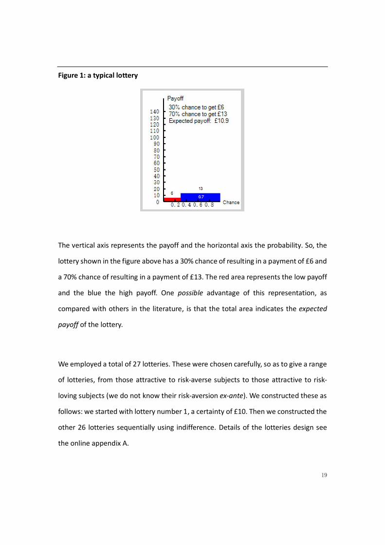
Figure 1: a typical lottery

The vertical axis represents the payoff and the horizontal axis the probability. So, the

lottery shown in the figure above has a 30% chance of resulting in a payment of £6 and

a 70% chance of resulting in a payment of £13. The red area represents the low payoff

and the blue the high payoff. One possible advantage of this representation, as

compared with others in the literature, is that the total area indicates the expected

payoff of the lottery.

We employed a total of 27 lotteries. These were chosen carefully, so as to give a range

of lotteries, from those attractive to risk-averse subjects to those attractive to risk-

loving subjects (we do not know their risk-aversion ex-ante). We constructed these as

follows: we started with lottery number 1, a certainty of £10. Then we constructed the

other 26 lotteries sequentially using indifference. Details of the lotteries design see

the online appendix A.

20

The experiment was designed in two parts. Part 1 elicited their ex-ante evaluation of

singleton lotteries by using (our slight modification of) Holt-and-Laury’s price list

method. From this, we can infer the ranking of singleton menus (that is, those

consisting of just one lottery). Part 2 consisted of two stages: first, subjects were asked

to choose one menu from three different menusets (sets of menus) of different sizes

and composition; second, they were asked to choose one lottery from the chosen

menu. Part 1 consisted of 27 tasks, and Part 2 consisted of 30 tasks. Note that the

menus and menusets in part 2 varied across subjects according to their evaluation of

the singletons in part 1. At the end of the experiment, one of the total of 57 tasks was

chosen at random, and the subject’s decision on that task was ‘played out’. Following

all models’ original menus as sets of lotteries, lotteries will be used to infer the risk

preference, and hence determine the preferences as defined in each model.

4.2 Eliciting the ex-ante preference on temptation free singleton lotteries

The evaluation of the ex-ante preference, which is a key component in most models

under consideration, cannot be observed from the two choices (choice of a menu and

choice from the menu) in the second part of the experiment. Thus, we elicited the ex-

ante risk attitude ur in the first part using (our slight modification of) the Holt and Laury

price-list mechanism. In this first part, we asked subjects to value each lottery:

subjects were told to imagine that they owned the lottery and planned to sell it; their

valuation is the smallest amount of money they would happily accept to sell it.

Alternatively, they were asked to imagine that they did not own the lottery and were

thinking of buying it; then the valuation is the largest amount of money they would

happily pay to buy it. Thus, their valuation depends on their own ex-ante risk attitudes.

21

This elicitation came before the subjects began to make decisions in Part 2 of the

experiment. In Part 1, we elicited each singleton valuation by showing a particular

lottery on the left of the screen and a drop-down list of numbers on the right. Subjects

indicated their valuation of the lottery on the left by ticking one of the numbers on the

right. The Instructions showed the interface; it is given in Appendix Figure 1.

To provide them with an incentive to reveal the true evaluation, we used the following

method to pay subjects if one of these lotteries was played out at the end of the

experiment: we randomly selected one of the numbers from the drop-down list; if that

number was less than the number they had ticked, we played out the lottery on the

left; if that number was equal to or greater than the number they had ticked, the

payment was the number that they have ticked.

4.3 Menu and temptation design

The implement of temptation was designed carefully. Temptation is a taste shock

where the individual’s future desire conflicts with their initial desire. We would like to

generalise the temptation as the existence of diverse and extremely different

problems that conflict with our initial preference. In our daily life, what distracts us

and motives us to change our preference is not always something strictly bad or wrong

in this information-exploration and choice-overload era. For example, we may have

impulsive shopping behaviour that we do not plan to do when we are seeing

something beautiful in a shop window. We may plan to have a risk neutral investment

portfolio, but we may be attracted by a high possible outcome to become more risk-

loving if the investment adviser offers a risky portfolio. Thus, in our experiment, we

designed some extremely safe and extremely risky problems as source of temptation.

22

As we have inferred the ex-ante preference ru the first stage, our experimental

software generated the menus accordingly. Thus, we designed the menus within each

menuset with different degrees of riskiness that deviate from their ex-ante risk

aversion. For example, each menu will have one or two lotteries close to subjects’ ex-

ante preference, that is, those that have an expected utility close to their maximum

expected utility given their ru; while some menus will have different lotteries with

different degrees of risk, which were usually extremely risky or safe problems

compared with their most ex-ante preferred lotteries.

4.4 Menusets

The menusets were carefully designed. Each menuset had three menus with different

sizes (to implement the flexibility and multiple temptations) – one menu had two

lotteries without temptations and these two lotteries which had close to the maximum

utility given by their ru; one menu had three lotteries with two ex-ante preferred

lotteries given their ru and one possibly tempting lottery; one menu had four lotteries

with two ex-ante preferred lotteries given their ru and two possibly tempting lotteries.

To incentivise subjects to trade off and evaluate the menus carefully, the menus did

not fully overlap each other: If the larger menus contain the lotteries of smaller menus,

subject may simply choose the larger size without thinking and decide the final

decision carefully at the last stage. So the temptation-free menu has the most

preferred lotteries given their ru; the larger menus with temptations have less

preferred lotteries given their ru.

Let us give an example. Suppose the estimated risk-aversion, ru, of a particular subject

is 0.32. Using the notation xpy to denote a lottery which leads to a payoff x with

23

probability p and to a payoff y with probability 1-p, then the lotteries 180.3697, 200.2538

and 180.4306 are closest to the subject’s ex-ante preferences; these are lotteries 14, 15

and 13 respectively (see Appendix Table 1 and Figure 2 above). We constructed a

menuset containing the menus below

A 14 15

B 14 13 1

C 15 13 1 27

Lottery 1 is the safest lottery and lottery 27 the riskiest; these are the furthest away

from the subject’s ex-ante preferences, and hence possibly the most tempting.

Meanwhile lotteries 13, 14 and 15 are the least tempting. Menusets were constructed

subject-by-subject using this design.

5. Stochastic Specification

The choice of menu stage in all models are deterministic stories, identifying a

particular optimal menu. In any experiment, however, there is behavioural noise:

subjects often choose differently when offered the same choice on several occasions.

This fact implies that we have to model choices of menus in a stochastic fashion;

otherwise no model can explain the data. The multinomial logit model (or Luce model)

is perhaps the most commonly used model of discrete choice to account for

behavioural stochasticity. With this model, behaviour does not behave in a fully

random way but follows a particular random pattern. According to this model, the DM

evaluates the problems with some noise. If the noise in the evaluation is additively

separable and independently distributed according to the extreme value distribution,

then the multinomial logit model emerges. We use Luce’s random model to add

experimental noise into the choice of menu models. This model assumes that

24

the probability of selecting one menu over another from a set of many menus is not

affected by the presence or absence of other menus in the same context. The choice

probability formula is given by the equation below.

i

j

U

i U

j

eP

e

Where Ui is the expected utility of menu i, j is any other menu in the menuset and λ

is a precision parameter which measures the amount of experimental noise, and

reflects the variance of the unobserved portion of utility.

Ui is determined by different parameters in each model (our parameters of interest).

The choice of menu in GP and CK is determined by the ex-ante preference u and the

temption preference v in the menu; thus ru and rv are our estimated parameters in GP

and CK. In Stovall and AS, each DM is postulated to have a belief about her or future

preferences with corresponding probabilities. We could not estimate each single

possible preference and the discrete probability; the parameters will be too many to

be identified6. To make the likelihood function more parsimonious, we instead assume

that the belief on temptation preference can be modelled by a continuous normal

distribution with mean μ and standard deviation σ. We estimate μ and σ in AS and

Stovall.

5.1 Model identifiability demonstrated through simulation

6 For example, each menu set has 5 lotteries allocated in different menus. If we estimate the preference of each single lottery, and the corresponding probability, we will need to estimate at least 10 parameters, and a precision parameter, which gives 11 in total.

25

As already discussed, GP, Stovall, and CK identify the same choice of menu in some

cases, and hence they may not be distinguishable. We demonstrate identifiability with

our Luce stochastic specification7 through a simulation.

In this simulation we have assumed that ru=0.32 and have used the corresponding

menusets generated as in our experiment as described above. We first generated

10000 sets of observations on the choice of a menu for the different models assuming

Luce noise. We then estimated the parameters of the different models. This was to see

if the maximum likelihood estimation can identify the true model that was used to

generate the decisions, and if the true parameters can be estimated. We use the BIC8

criterion to determine the best-fitting model. The results are in Tables 3 to 7.

Table 3: True Model is GP type 1

True Model is GP type 1 with parameters 1.7rv and 800

Mean estimated parameters are 1.698rv and 802.778

Estimated model

GP type 1 GP type 2 CK Stovall AS

Mean uncorrected log-

likelihood -139530 -145893 -144387 -150698 -329634

BIC 279084 291812 288811 301434 659274

7 Of course, this assumes that our subjects are noisy in their responses. 8 BIC is the Bayesian Information Criterion; this corrects the log-likelihood for the number of parameters.

26

Table 4: True Model is GP type 2

True Model is GP type 2 with parameters 1.7rv and 800

Mean estimated parameters are 1.888rv and 800.17

Estimated model

GP type 1 GP type 2 CK9 Stovall AS

Mean uncorrected log-

likelihood -107150 -106183 -106183 -119592 -329584

BIC 123949 122219 122232 321434 623274

Table 5: True Model is CK.

True Model is CK with parameters 1.7rv , 0.8q and 800 .

Mean estimated parameters are 1.83rv , 0.80q and 803

Estimated model

GP type 1 GP type 2 CK Stovall AS

Mean uncorrected likelihood -259048 -259300 -247961 -257452 -274653

BIC 518121 518625 495960 514941 549344

9 When the probability to be tempted is 1 in CK, the CK representation will become GP type 2. Thus, the likelihood of CK is the same as GP type 2 and estimated probability is 1. Note that the BIC of two models are different thus，we still can

identify the true model according to the lowest BIC

27

Table 6: True Model is Stovall

True Model is Stovall with parameters 1.2 , 10 and 800

Mean estimated parameters are 1.24 , 11.00 and 828.24 .

Estimated model

GP type 1 GP type 2 CK Stovall AS

Mean uncorrected likelihood -255119 -300144 -253231 -231355 -274670

BIC 510264 606314 506498 462747 549378

Table 7: True Model is AS

True model is AS with parameters 1.2 , 10 and 800 .

Mean estimated parameters are 1.19 , 12.81 and 789.22 .

Estimated model

GP type 1 GP type 2 CK Stovall AS

Mean uncorrected likelihood -327949 -329335 -329574 -329169 -308255

BIC 655923 658695 659185 658375 616548

The above tables show that using the Luce model, GP, CK, and Stovall are

distinguishable and identifiable. Obviously, AS is easily to be distinguished as it is

opposite to the other models.

28

5.2 Simulation of prediction

As mentioned, we also want to test the models’ predictive power to see which model’s

choice of menu stage better implies the choice from menu, and hence whether our

subjects were consistent. So we used the estimated parameters of the of stage to

predict behavior at the from stage, and compared the corresponding prediction log-

likelihoods. Our hypothesis is, that, if DMs are consistent across stages according to

the models, the model that fits the behavior at the choice of menu stage, should also

predict best the choice from menu stage given the same parameters. We report here

a simulation to test this hypothesis (which we will use in the results section). As we

have already noted, we cannot estimate AS and Stovall in our experiment due to the

limited number of observations, so only results for GP and CK are reported here.

Table 8: True Model is GP type 1

True Model is GP type 1 with parameters 1.7rv and 800

Mean estimated parameters are 1.698rv and 802.778

Predicted models of from

GP type 1 GP type 2 CK

Mean uncorrected log-likelihood -67435 -97908 -119916

29

Table 9: True Model is GP type 2

True Model is GP type 2 with parameters 1.7rv and 800

Mean estimated parameters are 1.89rv and 799.14

Predicted models of from

GP type 1 GP type 2 CK

Mean uncorrected log-likelihood -50378 -43021 -44498

Table 10: True Model is CK

True Model is CK with parameters 1.7rv , 0.8q and 800 .

Mean estimated parameters are 1.83rv , 0.80q and 803

Predicted models of from

GP type 1 GP type 2 CK

Mean uncorrected log-likelihood -237088 -242278 -201484

Tables 8 to 10 show clearly that, if DMs are consistent in terms of preference, the true

model has the higher log-likelihood. Hence, the predictive powers can be compared

and the true generating model identified. We use this in our results section.

6. Results

In this section, we present the experimental results from the experiment conducted at

EXEC, the Centre for Experimental Economics at the University of York, in 2021. A total

30

of 82 subjects (mainly students) participated in the experiment10and mean earnings

were £23.50 per subject (including a £2.50 show-up fee).

6.1 Flexibility and temptation: some descriptive statistics

Overall, the frequency to choose size 2 menus (that is, menu 1) was 32%, the frequency

to choose size 3 menus (that is menu 2) was 22%, and that to choose size 4 menus

(menu 3) was 46%. In the temptation menu sets, the frequency to choose size 2 menus

(menu 1) was 27% ,the frequency to choose size 3 menus (menu 2) was 14% , and that

of size 4 (menu 3) was 59% (see Table 9).

Table 11: the frequency to choose each menu

Menusets type menu 1 menu 2 menu 3

temptation free menusets 0.32 0.22 0.46

(0.24) (0.19) (0.26)

temptation menusets 0.27 0.14 0.59

(0.19) (0.16) (0.25)

Each subject completed 30 tasks, each involving a choice of a menu and a choice from

the chosen menu. We start with some descriptive statistics. In order to test if subjects

are tempted by our designed temptations, we included in the menusets, 5 menusets

that contained temptation-free menus where there are no tempting lotteries.

Comparing average frequencies to choose different sizes of menus (see Table 11), we

can see that subjects had a relative higher tendency to choose the flexible menu where

10 Due to covid 19, we conducted our experiments online in our virtual lab.

31

there were temptations. Note that menu 2 has one temptation, while menu 3 has two

temptations.

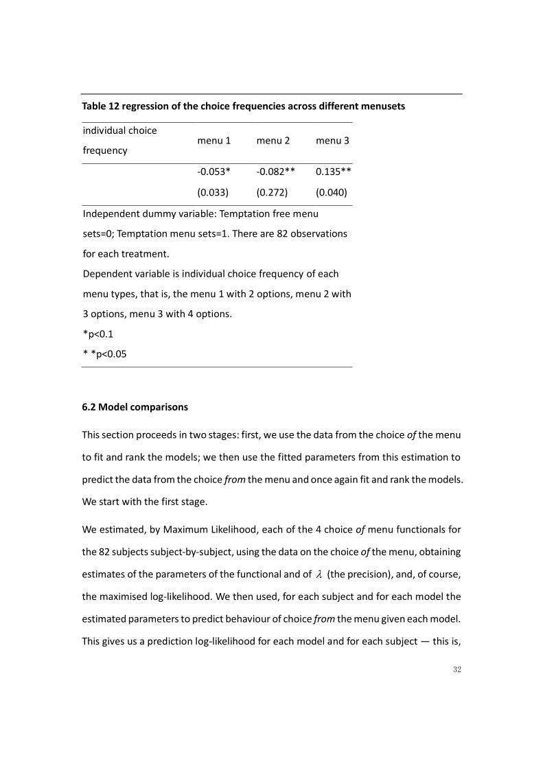
We report in Table 12 on a regression of the choice frequencies across different

menuset contexts to see the relation between choice frequencies of different menus

and temptation (free) menu set. If our implementation of temptation worked, subjects

will have higher tendency to choose larger menus in temptation menusets than in

temptation-free menusets, and correspondingly higher tendency to choose smaller

menus in temptation-free menusets than temptation menusets. According to table 8,

the individual choice frequency of menu 3 in the temptation menu set is significantly

higher than that of temptation free menuset. Accordingly, the tendency to choose

menu 1 is significantly lower in temptation menusets than in the temptation-free

menu sets. These results show that our method to design the temptation do tempt

the subject to give into the menu with more temptations and choose flexibility. Our

conclusion from this descriptive data is that the way that we have designed our

menusets is valid.

32

Table 12 regression of the choice frequencies across different menusets

individual choice

frequency menu 1 menu 2 menu 3

-0.053* -0.082** 0.135**

(0.033) (0.272) (0.040)

Independent dummy variable: Temptation free menu

sets=0; Temptation menu sets=1. There are 82 observations

for each treatment.

Dependent variable is individual choice frequency of each

menu types, that is, the menu 1 with 2 options, menu 2 with

3 options, menu 3 with 4 options.

*p<0.1

* *p<0.05

6.2 Model comparisons

This section proceeds in two stages: first, we use the data from the choice of the menu

to fit and rank the models; we then use the fitted parameters from this estimation to

predict the data from the choice from the menu and once again fit and rank the models.

We start with the first stage.

We estimated, by Maximum Likelihood, each of the 4 choice of menu functionals for

the 82 subjects subject-by-subject, using the data on the choice of the menu, obtaining

estimates of the parameters of the functional and of (the precision), and, of course,

the maximised log-likelihood. We then used, for each subject and for each model the

estimated parameters to predict behaviour of choice from the menu given each model.

This gives us a prediction log-likelihood for each model and for each subject — this is,

33

of course, a measure of the predictive abilities of the models. We did this for GP and

CK, because these two models predict different choices from the menu even though

they indicate the same choice of menu. Doing so enables us to discriminate between

the two models.

We start with Table 13; this shows the mean and standard deviation (across all subjects)

of the fitted log-likelihoods. However, this table does not allow us to compare the

goodness of fit across preference functionals, for the simple reason that they have

different degrees of freedom (GP has 2 estimated parameters, CK 2, Stovall 3, and AS

3). If we correct the fitted log-likelihoods for the degrees of freedom by calculating the

Bayesian Information Criterion (BIC), we get the bottom half of Table 9; recall that the

lower the BIC the better. It seems to show that, on average, CK is the best, followed by

GP, and then AS and Stovall.

Table 13 (mean and standard deviation of maximised log-likelihoods and the values

of BIC)

GP11 AS CK Stovall

uncorrected likelihoods -30.58 -29.34 -23.52 -32.66

(4.53) (3.45) (7.73) (0.74)

BIC 69.35 70.96 55.23 77.61

(9.06) (6.90) (15.46) (1.47)

11 GP models two types of subjects, self-control and temptation overwhelming. We identify the type by the higher maximised likelihood since two types have the same number of parameters. 78.2% subjects are identified as self-control type and 21.8% are temptation overwhelming subjects.

34

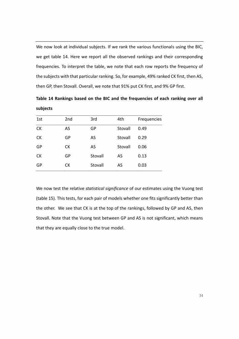
We now look at individual subjects. If we rank the various functionals using the BIC,

we get table 14. Here we report all the observed rankings and their corresponding

frequencies. To interpret the table, we note that each row reports the frequency of

the subjects with that particular ranking. So, for example, 49% ranked CK first, then AS,

then GP, then Stovall. Overall, we note that 91% put CK first, and 9% GP first.

Table 14 Rankings based on the BIC and the frequencies of each ranking over all

subjects

1st 2nd 3rd 4th Frequencies

CK AS GP Stovall 0.49

CK GP AS Stovall 0.29

GP CK AS Stovall 0.06

CK GP Stovall AS 0.13

GP CK Stovall AS 0.03

We now test the relative statistical significance of our estimates using the Vuong test

(table 15). This tests, for each pair of models whether one fits significantly better than

the other. We see that CK is at the top of the rankings, followed by GP and AS, then

Stovall. Note that the Vuong test between GP and AS is not significant, which means

that they are equally close to the true model.

35

Table 15 significance tests of comparative model fit

H0: Model 1 and model 2 are equally close to the true model

H1: Model 1 is closer to the true model than model 2

model 1/model 2 GP AS CK Stovall

GP - 1.216 -4.101 8.267

AS -1.216 - -5.821 5.896

CK 4.101 5.821 - 6.812

Stovall -8.267 -5.896 -6.812 -

-has no meaning

If V> 1.96, model 1 is significantly better than model 2；

If V< -1.96 model 2 is significantly better than model 1；

If |V| < 1.96 model 1 and model 2 are equally close to true model.

6.3 The predictive power of each model

The above analyses are concerned with the explanatory ability of each model in the of

stage. Now we check the predictive power in the from stage for GP and CK12. As can be

seen from Table 15, GP and CK come out well in the fitting of the of stage. We now

want to see which of the two can predict best the behavior at the from stage. We start

with the estimated parameters from the of stage. GP and CK both predict a choice from

the menu, which depends upon the parameters in the of stage. We used, for both

models, and for each subject the estimated parameters from the of stage to predict

behaviour on the choice from the menu (using the two models’ model’s implied

behaviour functionals and corresponding choices. This gives us a prediction log-

12 As mentioned earlier, we have difficulty in estimating the from stage of AS and Stovall since we do not have enough data.

36

likelihood for each functional and for each subject — this is, of course, a measure of

the predictive ability of the theory. We add noise into the choice in the from stage

once again using the Luce method, since GP’s and CK’s modelling of the from stage are

deterministic. Since the decision context is different, we assume that the noise

parameters at the choice from the menu stage are different from those at the choice

of the menu stage.

Table 16 Mean log-likelihood of choice from menu (standard deviation in

parentheses)

GP CK

fitted likelihood -59.37 -23.52

(8.96) (3.45)

According to table 16, CK emerges as the best in this prediction contest13. To check

the significance, we use the Vuong test, as before. The results are in Table 17. This

shows that CK fits significantly better than GP.

13 We also examined the results subject-by-subject; all subjects have a higher prediction log-likelihood with CK than with GP.

37

Table 17 significance tests of comparative model fit

H0: Model 1 and model 2 are equally close to the true model

H1: Model 1 is closer to the true model than model 2

model 1/model 2 GP CK

GP - -8.512

CK 8.512 -

- No meaning

If V> 1.96, model 1 is significantly better than model 2；

If V< -1.96 model 2 is significantly better than model 1；

If |V| < 1.96 model 1 and model 2 are equally close to true model.

7. Conclusions

We report on an experimental investigation into the relative explanatory and

predictive power of four prominent theoretical models of two-stage decision-making.

These models are ones in which the decision maker (DM) makes a choice of a menu in

the first stage and then makes a choice from the chosen menu in the second stage.

The models considered are those of GP (Gul and Pesendorfer, 2001), Stovall (2010), CK

(Chatterjee and Krishna, 2009) and AS (Ahn and Sarver, 2013).

The experiment and particularly the menus were carefully designed so that temptation,

the cost of self-control, possible multiple temptation and flexibility were all

incorporated. In estimation, we use the Luce stochastic specification to incorporate

experimental noise, and hence render the models distinguishable14 (identifiable).

14 AS is distinguishable because of its differences.

38

Our parametric estimation results show that CK generally explains better than the

other models, and also predicts better the choice from the menu than GP. GP and AS

are ranked second on the choice of the menu (with their explanatory powers not

significantly different) while Stovall performs worst.

In our experiment, we use lotteries as the final objects of choice, and define

preferences in terms of the attitude towards risk of the subjects. We follow the

literature in identifying ex ante preferences as those applying to the preferences at the

start of the decision process, and ex post preferences as those applying when the final

decision from the chosen menu is made. Conflicts arise when ex post preferences

depart from ex ante preferences. This raises questions of dynamic consistency, and

hence questions as whether the DM anticipates that there may be this departure.

CK models a particularly simple decision-maker who acts as if her final choice will be

probabilistically made either on the basis of her ex ante preferences or on the basis of

her ex post preferences; in the latter case, the DM, in the language of the literature,

“succumbs” to the temptation of her ex post preferences; the DM anticipates her

behaviour in the choice of the menu. In contrast, GP posits a more sophisticated DM

who anticipates a struggle at the second stage, and takes into account the cost of this

struggle when deciding at the first stage. In stark contrast to this story, AS posits a DM

who totally ignores her ex ante preferences, and bases her decision at the first stage

solely on the basis of her possible ex post preferences. Whereas, in Stovall the DM

anticipates her possible second-stage decisions (which will be based on her ex post

preferences) and evaluates them according to her ex ante preferences.

In our experimental context, we define the final objects of choice as lotteries with

differing degrees of risk. Thus, particular choices are not necessary strictly better or

39

worse than others; this depends on the DM’s attitude to risk. This is in contrast to the

few self-control and temptation experiments, where the temptation and choice

contexts are usually specified and clearly defined as bad or good ̶ such as a willingness

to read gossip (Toussaert, 2018), and using the internet when doing tedious work

(Houser et al, 2010); In these contexts, the motivation of self-control may not be strong

and clear enough. We mainly focus on preference consistency. Thus, rather than in the

deterministic self-control of GP, in the random indulgence model of CK the DM

perceives a positive probability to succumb to the temptation, where there are (ex-

ante) costs from succumbing. It seems that the uncertainty in CK’s model accounts for

behaviour in our experiment. Compared to the uncertainty of CK, Stovall incorporates

uncertainty driven by multiple temptations. Thus, all possible temptations, and not

just the most tempting option, will be taken into consideration. However, we do not

know if subjects are tempted by multiple temptations in our experiment. We can only

infer that the existence of extremely risky or safe options tend to tempt the DM, but

do not know if the subjects are tempted by one of them or by both. Stovall does not

work well compared with the other models, perhaps due to our design.

In the light of our estimation results, we can answer our three main questions

proposed earlier.

First, whether the strength of ex-ante preference or preference flexibility is prevalent

in reality? In our experiment, subjects tended to keep ex-ante preferences and remain

consistent as long as they were not tempted to reverse their preference. As discussed,

only AS addresses a preference for flexibility, where ex-ante preference does not

impinge on subsequent decisions. According to Table 14, the vast majority of subjects’

decisions are best explained by CK, with a small minority explained by GP, in which the

ex-ante preference plays a crucial role. Our results offer insight into choice-overload

40

and preference-consistency research: if the more flexible choice set conflicts with long

term normative preference, having more choices is not necessarily better. As

mentioned earlier, AS and Stovall consider all possibilities of future preferences due to

uncertainty while CK and GP only identify the most tempting one. We can conclude

from our results that only the most attractive option influences decision making in our

context.

Second, as to whether adding middle level problems influences the utility of a menu,

we cannot draw a conclusion, since we cannot know if our designed multiple

temptations do tempt the subjects simultaneously. Our results raise the following

question for future research: when there are multiple diverse options, can subjects be

tempted by multiple extremely conflicting options at the same time?

Third, for GP and CK we can conclude that CK better predicts the choice from the menu;

but our data is insufficient for a conclusion with respect to AS and Stovall.

Overall, our results come down firmly in concluding that CK is the better model of the

four. This could result because of the simplicity of CK: the DM probabilistically either

sticks with her ex-ante preferences or switches to her ex post preferences. It is a simple

story, almost a heuristic, though it is justified by an axiomatic derivation. If one could

test axioms directly, it would be interesting to discover which axiom is the crucial one.

41

References

Ahn, D. and Sarver, T., 2013. Preference for Flexibility and Random

Choice. Econometrica, 81(1), pp.341-361.

Amador, M., Werning, I. and Angeletos, G., 2003. Commitment vs. Flexibility. SSRN

Electronic Journal,

Chatterjee, K. and Krishna, R., 2009. A “Dual Self” Representation for Stochastic

Temptation. American Economic Journal: Microeconomics, 1(2), pp.148-167.

Dekel, E. and Lipman, B., 2012. Costly Self-Control and Random Self-

Indulgence. Econometrica, 80(3), pp.1271-1302.

Dekel, E., Lipman B. and Rustichini, A., 2009. Temptation-Driven Preferences. Review

of Economic Studies, 76(3), pp.937-971.

Gul, F. and Pesendorfer, W., 2001. Temptation and Self-Control. Econometrica, 69(6),

pp.1403-1435.

Houser, D., Schunk, D., Winter, J. and Xiao, E., 2010. Temptation and Commitment in

the Laboratory. SSRN Electronic Journal,

Koida, N., 2017. Anticipated stochastic choice. Economic Theory, 65(3), pp.545-574.

Kreps, D., 1979. A Representation Theorem for "Preference for

Flexibility." Econometrica, 47(3), p.565.

Ortoleva, P., 2013. The price of flexibility: Towards a theory of Thinking

Aversion. Journal of Economic Theory, 148(3), pp.903-934.

Stovall, J., 2010. Multiple Temptations. Econometrica, 78(1), pp.349-376.

42

Toussaert, S., 2018. Eliciting Temptation and Self-Control Through Menu Choices: A Lab

Experiment. Econometrica, 86(3), pp.859-889.