NBER WORKING PAPER SERIES

STOCK-MARKET CRASHES AND DEPRESSIONS

Robert J. BarroJosé F. Ursúa

Working Paper 14760http://www.nber.org/papers/w14760

NATIONAL BUREAU OF ECONOMIC RESEARCH1050 Massachusetts Avenue

Cambridge, MA 02138February 2009

This research is supported by a grant from the National Science Foundation. The views expressedherein are those of the author(s) and do not necessarily reflect the views of the National Bureau ofEconomic Research.

© 2009 by Robert J. Barro and José F. Ursúa. All rights reserved. Short sections of text, not to exceedtwo paragraphs, may be quoted without explicit permission provided that full credit, including © notice,is given to the source.

Stock-Market Crashes and DepressionsRobert J. Barro and José F. UrsúaNBER Working Paper No. 14760February 2009JEL No. E01,E21,E23,E44,G01,G12

ABSTRACT

Long-term data for 25 countries up to 2006 reveal 195 stock-market crashes (multi-year real returnsof -25% or less) and 84 depressions (multi-year macroeconomic declines of 10% or more), with 58of the cases matched by timing. The United States has two of the matched events—the Great Depression1929-33 and the post-WWI years 1917-21, likely driven by the Great Influenza Epidemic. 45% ofthe matched cases are associated with war, and the two world wars are prominent. Conditional ona stock-market crash, the probability of a minor depression (macroeconomic decline of at least 10%)is 30% and of a major depression (at least 25%) is 11%. In a non-war environment, these probabilitiesare lower but still substantial—20% for a minor depression and 3% for a major depression. Thus,the stock-market crashes of 2008-09 in the United States and other countries provide ample reasonfor concern about depression. In reverse, the probability of a stock-market crash is 69%, conditionalon a depression of 10% or more, and 91% for 25% or more. Thus, the largest depressions are particularlylikely to be accompanied by stock-market crashes, and this finding applies equally to non-war andwar events. We allow for flexible timing between stock-market crashes and depressions for the 58matched cases to compute the covariance between stock returns and an asset-pricing factor, whichdepends on the proportionate decline of consumption during a depression. If we assume a coefficientof relative risk aversion around 3.5, this covariance is large enough to account in a familiar lookingasset-pricing formula for the observed average (levered) equity premium of 7% per year. This findingcomplements previous analyses that were based on the probability and size distribution of macroeconomicdisasters but did not consider explicitly the covariance between macroeconomic declines and stockreturns.

Robert J. BarroDepartment of EconomicsLittauer Center 218Harvard UniversityCambridge, MA 02138and NBERrbarro@harvard.edu

José F. UrsúaDepartment of EconomicsLittauer Center 218Harvard UniversityCambridge, MA 02138jfursua@fas.harvard.edu

“The stock market has predicted nine of the last five recessions,” Samuelson (1966).

The Samuelson quote is remarkable because it is simultaneously extremely clever and

extremely misleading. We find, for 25 countries with long-term data, that stock-market crashes

(cumulated multi-year real returns of -25% or less) go along with minor depressions (multi-year

declines of consumption or GDP by 10% or more) 30% of the time and major depressions

(declines by 25% or more) 11% of the time. In reverse, minor depressions feature stock-market

crashes 69% of the time, whereas major depressions feature these crashes 91% of the time.

Thus, as the Samuelson quote suggests, stock-market crashes are far more frequent than

depressions. Nevertheless, a stock-market crash provides good reason for concern about the

macro economy—because the conditional 30% chance of a minor depression and 11% chance of

a major depression are far above the typical probabilities. In reverse, the absence of a stock-

market crash is reassuring in the sense that a depression is highly unlikely.

The overall probability of moving from a “normal state” into a minor depression turns out

to be 3.7% per year (3 per century). But knowing that there is no stock-market crash lowers the

odds to 1.0% per year (1 per century). For a major depression, the overall probability is 0.9%

per year (1 per century), but conditioning on no stock-market crash reduces this chance to 0.08%

per year (less than 1 per millennium). Hence, although Samuelson is right in some sense, stock

returns still provide important guidance about the prospects for depression. This kind of

information is particularly valuable in the financially turbulent environment of 2008-09.

2

I. Stock-Market Crashes and Depressions in the Long-Term International Data

This study uses an updated version of the macroeconomic and stock-return data described

in Barro and Ursua (2008). For the macroeconomic aggregates, we have annual time series from

before 1914 for real per capita consumer expenditure, C, for 24 countries and real per capita

GDP for 36 countries. Our earlier study and the online information available at

http://www.economics.harvard.edu/faculty/barro/data_sets_barro provide a detailed description

of the methods and sources used to construct the data on C and GDP.1

For stock returns, the data come mainly from Global Financial Data (described in Taylor

[2005]).2 When available, we used nominal total return indexes, deflated by consumer price

indexes, to compute annual, arithmetic real rates of return. In other cases, we used nominal

stock-price composite indexes, deflated by consumer price indexes, and then added estimates (or

sometimes actual values) of dividend yields to estimate the arithmetic real rates of return. The

present study focuses on 25 countries (18 OECD) with annual stock-return data since at least the

early 1930s. Our annual real rates of return apply from the end of the previous year to the end of

the current year.3

As in Barro and Ursua (2008), we gauge “depressions” by peak-to-trough declines in real

per capita consumer expenditure, C, or GDP. These declines can apply to multiple years, such as

1 Barro and Ursua (2008) compare our GDP data with those in Maddison (2003). One problem with the Maddison

data is his propensity to interpolate in poorly documented ways over periods with missing data. 2 We use the data from Dimson, Marsh and Staunton (DMS), available through Morningstar, for Canada 1900-13,

Denmark 1900-14, Italy 1900-05, Netherlands 1900-19, Sweden 1900-01, Switzerland 1900-10, and South Africa

1900-10. We use stock-price data for Japan 1893-1914 from Fujino and Akiyama (1977) and for Mexico 1902-29

(missing 1915-18) from Haber, Razo, and Maurer (2003). Care should be taken in using the DMS data for later

periods, usually wars, with missing entries in Global Financial Data. These DMS data appear to be generated (for

periods such as France 1940 and Portugal 1974-77 when stock-return data seem to be unavailable) by interpolation.

We have not used any of this information. 3 For cases of missing data, usually during wars and sometimes because of closed markets, we were able to compute

cumulative multi-year real returns across the gaps. These cases are Belgium 1914-18 and 1944-46, France 1940-41,

India 1926-27, Mexico 1915-18, Netherlands 1944-46, Spain 1936-40, Portugal 1974-77, and Switzerland 1914-16.

3

1912 to 1918 for Germany during World War I, 1929 to 1933 for the U.S. Great Depression,

1935 to 1937 during the Spanish Civil War, 1938 to 1943 for France in World War II, 1972 to

1976 covering the Pinochet coup in Chile, 1981 to 1988 in Mexico during the Latin American

debt crisis, and 1989 to 1993 during the financial crisis in Finland.4 In the main analysis, we

follow our previous study in focusing on contractions in C or GDP of size 0.10 or more.

However, we also consider higher thresholds for labeling an economic decline as a depression.

In terms of asset pricing, the analysis maps more closely to consumption than to GDP.

However, our C measures refer, because of data availability, to personal consumer expenditure,

rather than consumption. Moreover, in many cases, the measurement error in C is likely to be

greater than that in GDP. The analysis in Barro and Ursua (2008, section V) found that major

contractions in C and GDP were similar overall in terms of timing. The average proportionate

size of contraction was also similar during non-war periods. However, because of the large

expansion in military purchases during wars, the average proportionate contraction in C during

wartime was, on average, five percentage points greater than that in GDP. For example, the

United Kingdom had depressions gauged by C during the two world wars but not by GDP.

Moreover, some non-war aftermaths, such as the United States from 1944 to 1947, featured

substantial declines in GDP but not in C—because of the massive demobilization that featured

sharp declines in military purchases. This kind of post-war case does not constitute a depression

in an economic sense.

Putting these results together, we decided to measure macroeconomic contractions during

non-war years as the average of those found in C and GDP. (If only one of the variables was

4 In Barro and Ursua (2008) and in our main analysis here, we sometimes have intermediate years with small

increases in C or GDP. However, the results do not change a lot if we constrain multi-year contractions to have

declines in C or GDP for every year included in the multi-year interval.

4

available—in practice, GDP but not C—we gauged the contraction by the available variable.) In

war aftermaths, we used only the information on C (and left the data as missing when only GDP

was available). In war periods, we typically used only the data on C. However, we used an

average of C and GDP when the contraction indicated by GDP was larger or when only the GDP

data were available and the indicated contraction size was at least 0.10. For the 25 countries in

the present study (2652 annual observations), this procedure yields 84 cases of macroeconomic

contraction of size 0.10 or more.

We now apply an analogous peak-to-trough procedure to gauge stock-market crashes. In

our main analysis, we focus on cumulative, multi-year real returns that were -0.250 or less. For

the 25 countries, this procedure yields 195 cases of stock-market crashes.

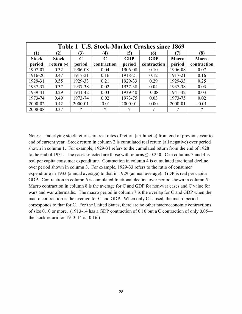
Table 1 illustrates our methodology for U.S. data since 1869. We found 7 stock-market

crashes (not including 2008, since our main sample goes to 2006), using the definition of

cumulative real returns of -0.250 or less.5 The worst is -0.55 for 1929-31 (Great Depression),

followed by -0.49 for 1973-74, -0.47 for 1916-20, and -0.42 for 2000-02. The value -0.37 for

2008 (using data only through 2008) would be worth fifth place if it were included in the sample.

The others are -0.37 for 1937-38, -0.32 for 1906-08, and -0.29 for 1939-41.

We matched stock-market crashes with depressions (macroeconomic contractions of size

0.10 or more) by finding periods that were coincident or adjacent. Table 1 illustrates our general

procedure by providing the details for the United States from 1869 to 2006. The first two

columns refer to the stock-market crashes, of which there were seven up to 2006 (and one more

for 2008). The “macro contraction” in columns 7 and 8 is calculated by the method described

5 The October 1987 U.S. stock-market crash does not show up as a decline for the full year. However, 1987 does

appear as a sharp fall in the annual data for many other countries, including France, Germany, Italy, Denmark,

Norway, Switzerland, and India.

5

earlier from the C and GDP declines shown in columns 3-6. The United States from 1869 to

2006 experienced only two periods with macro contractions of size 0.10 or more—the Great

Depression of 1929-33, with a contraction of 0.25, and 1917-21, with a decline by 0.16. As

discussed in Barro and Ursua (2008, section III), the 1917-21 contraction likely reflects the Great

Influenza Epidemic, rather than World War I, per se. The other five periods with stock-market

crashes were not associated with depressions, although 1906-08 comes close, 1937-38, 1973-74,

and 2000-01 are all recession periods, and 1941-42 shows a decline in C but not in GDP. Of

course, we do not yet know what will happen in the years following 2008. Note also that, unlike

many other countries, the United States from 1869 to 2006 had no depressions that were not

associated with stock-market crashes.

We applied the same methodology to all 25 countries (18 OECD) with long-term data on

stock returns and the macroeconomic variables (at least GDP).6 The matching of periods of

stock-market crashes with those of macroeconomic declines were sometimes less clear cut than

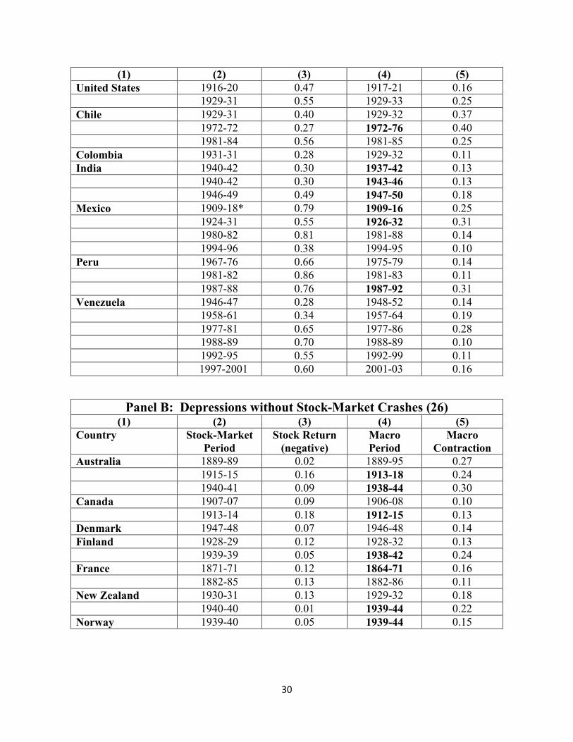
for the United States, but these considerations appear to be minor overall. Table 2, Panel A lists

the 58 cases of stock-market crashes (returns of -0.250 or less) that paired up with depressions

(macro contractions of 0.10 or more)—as already noted, two of these are for the United States.

In this sample, the average stock return was -0.53, with an average duration of 3.9 years, and the

average depression size was 0.23, with an average duration of 4.3 years.

Panel B lists the 26 cases of depressions that were not associated with stock-market

crashes—of which there were none for the United States. In this sample, the average stock

return was -0.09, with an average duration of 1.7 years, and the average depression size was

6 We included two countries, New Zealand and South Africa, that have long-term data on GDP but not C. Also, in

many cases, the GDP data start before the C data.

6

0.17, with an average duration of 4.0 years. There are another 137 cases (5 for the United States)

of stock-market crashes not associated with depressions, but these are not shown in the table.

The average stock return in this group was -0.41, with an average duration of 2.9 years, and the

average depression size was 0.01, with an average duration of 1.5 years.

Among the 58 cases of paired stock-market crashes and depressions shown in Table 2,

panel A, 14 are associated with World War II (including the neutral countries Spain, Sweden,

and Switzerland), 10 with the Great Depression of the early 1930s, and 9 with World War I

(including Sweden and Switzerland). There are 6 pairings associated with the Latin American

debt crisis of the 1980s, 7 other post-World War II cases in Latin America, and 5 events with

troughs in 1920-21, likely reflecting the Great Influenza Epidemic. The other cases involve

Japan during the Russo-Japanese War (1904-05), the Mexican Revolution and Civil War

(1910-20), the culmination of the German hyperinflation (1922-23), the Spanish Civil War

(1936-39), India during the post-WWII conflict with Pakistan (1947-48), the peaceful

(“Carnation”) revolution in Portugal (1974-75), and the early 1990s financial crisis in Finland.

In Table 2, a bold entry for the macroeconomic period indicates a time of war (defined to

include only active combatants).7 Overall, 45% of the cases in Panel A (26 of 58) are associated

with war.

Table 2, panel A misses a number of paired stock-market crashes and depressions

associated with the Asian financial crisis of the late 1990s because the countries involved lack

the long-term stock-return data needed to qualify for our sample. For example, Indonesia has a

7We used Correlates of War, inter- and intra-state conflicts (Sarkees [2000]), and other sources to designate times of

“major” war. In Table 2, the conflicts designated as war for active combatants are Franco-Prussian War 1870-71,

Russo-Japanese War 1904-05, World War I 1914-18, Mexican Revolution and Civil War 1909-18, Mexican War of

the Cristeros 1926-29, Spanish Civil War 1936-39, World War II 1939-45, India-Pakistan War 1947-48, Pinochet

coup in Chile 1973, Portugal Carnation Revolution 1974-75, and Peru’s guerrilla conflicts 1987-92.

7

stock return of -0.69 for 1997-98 and a macro contraction of 0.11 for 1997-98, South Korea has a

stock return of -0.63 for 1995-97 and a macro contraction of 0.11 for 1997-98, Malaysia has a

stock return of -0.54 for 1997-98 and a macro contraction of 0.11 for 1997-98, and Thailand has

a stock return of -0.81 for 1995-98 and a macro contraction of 0.14 for 1996-98. Our sample

also excludes recent cases in Russia and other former Communist countries that lack long-term

data.

In Table 2, panel B, for the 26 cases of depression unaccompanied by stock-market

crashes, 7 are related to World War II (including the neutral country Portugal), 5 with the Great

Depression, 4 with World War I (including the neutral country Chile), and 1 probably with the

Great Influenza Epidemic. Other cases were the depression in Australia in the early 1890s,

Canada in 1906-08 (likely related to the U.S. financial panic of 1907), Mexico in the early 1920s,

Denmark in 1946-48, France around 1871 (Franco-Prussian War), France in the 1880s, Portugal

at the time of the Spanish Civil War in 1934-36, Spain in the 1890s, and South Africa in the mid

1980s (possibly related to international sanctions against Apartheid). Overall, 31% of these

cases (8 of 26) are associated with war. In contrast, for the 137 cases of stock-market crashes not

associated with depressions, only 11 (8%) are associated with war.

II. Frequencies of Stock-Market Crashes and Depressions

Table 3 shows the overall frequency of stock-market crashes, defined as cumulative

multi-year returns of -0.250 or less—or, as an alternative, -0.300 or less. The table also shows

the frequency of macroeconomic contractions, defined as cumulative multi-year declines by at

8

least 0.10, 0.15, 0.20, 0.25, or 0.30. Part A of the table combines non-war and war observations,

and Part B distinguishes non-war from war events.

Begin with Part A of Table 3 and consider the pairing (-0.250, 0.10), which was used

before. By this definition, the overall sample (25 countries, 2652 annual observations) has 195

stock-market crashes and 84 macro contractions. The average durations were 3.2 years for the

stock-market crashes and 4.2 years for the macro contractions. When expressed as a probability

per year of moving from “normalcy” into each state, the values are 0.100 for the stock-market

crashes and 0.037 for the macro contractions. Thus, as Samuelson suggested, stock-market

crashes are far more frequent than depressions—reflecting the much greater volatility of stock

returns than of consumption or GDP growth rates.

Among the 195 stock-market crashes and 84 macro contractions, Table 3, part A shows

that 58 were matched events—occurring over overlapping or adjacent years. Thus, 30% and

69%, respectively, of the stock-market crashes and macro contractions are paired with the other

decline. To put it another way, if one knows that a stock-market crash (return of -0.250 or less)

occurred, it is 30% probable that a depression (of size 0.10 or more) also occurred. Conversely,

it one knows that a depression (of size 0.10 or more) occurred, it is 69% probable that a stock-

market crash (of size -0.250 or worse) also occurred.

Not surprisingly, the probability of depression, conditional on observing a stock-market

crash, declines as one raises the standard for declaring a depression. Table 3, part A indicates

that, conditional on a stock-market crash (-0.250 or worse), the probability of depression is 0.30

for size 0.10 or more, 0.18 for size 0.15 or more, 0.13 for size 0.20 or more, 0.11 for size 0.25 or

more, and 0.07 for size 0.30 or more.

9

In the reverse direction, the probability of a stock-market crash, conditional on seeing a

depression, becomes larger the higher the standard for labeling a macro contraction as a

depression. Table 3, part A shows that the conditional probability of a stock-market crash

(-0.250 or less) goes from 0.69 when depressions are of size 0.10 or more to 0.71 at 0.15, 0.74 at

0.20, 0.91 at 0.25, and 0.93 at 0.30. Thus, the largest depressions are almost surely accompanied

by stock-market crashes. (Table 2, panel B shows that the two largest depressions not

accompanied by stock-market crashes were in Australia—in the early 1890s and during World

War II.) Another way to view the result is that, if one knows that there is no stock-market crash,

it is extremely unlikely that a major depression exists.

The last result can be expressed by calculating probabilities per year of entering into

various states. Without knowing whether there is a stock-market crash, the unconditional

probability per year of moving from “normalcy” into a major depression (0.25 or more) is 0.0091

per year, a little less than 1 per century. Knowing that there is no stock-market crash lowers

these odds by a factor of 10 to 0.0008 per year, less than 1 per millennium. The change is less

dramatic if one considers depressions of size 0.10 or more. In this case, the unconditional

probability per year of entering into a depression is 0.037 per year (3-4 per century), whereas

conditioning on no stock-market crash lowers the chance to 0.010 per year (1 per century). In

other words, the conditioning reduces the depression odds by a factor of roughly four.

Table 3, part A also considers the breakpoint of -0.300 or less for declaring a stock-

market crash. The number of these larger crashes is 159, corresponding to a probability of 0.078

per year of entering into this state. Among the 84 macro contractions of size 0.10 or more, 48

(57%) are paired with a stock-market crash of -0.300 or worse. Conditional on observing a

10

stock-market crash of this larger magnitude, the probability of seeing a depression (0.10 or more)

is roughly the same as before, 0.30.

Table 3, part A also has results for samples limited to the 18 OECD countries. The

patterns are similar to those for the group of 25 countries. Thus, in the sample that combines

non-war and war events, the predictive element of a stock-market crash is about the same in

developed countries as in a set of middle-income countries from Latin America and Asia

(although stock returns and growth rates of macroeconomic aggregates are more volatile in the

middle-income countries).

Table 3, part B shows the results that separate non-war from war events. In the non-war

sample, considered in columns 3-5 of the table, the biggest change from before is the decrease in

depression probability, conditional on seeing a stock-market crash. For all 25 countries, for a

stock-market crash of -0.250 or worse, the conditional probability of a minor depression (0.10 or

more) is now 0.20, compared to 0.30 in the combined sample, and of a major depression (0.25 or

more) is 0.03, rather than 0.11. For the OECD, the change is more pronounced—the conditional

probability of a minor depression is now 0.17, rather than 0.28, and of a major depression is

0.02, rather than 0.10. The sample of OECD non-war events has only three major depressions—

Australia in the 1890s (which did not have a stock-market crash) and the Great Depression in

Canada and the United States (which had stock-market crashes).

We can apply the last set of findings to the 2008-09 environment, in which many

countries experienced stock-market crashes (returns of -0.250 or worse) but not major wars. In

this context, the upper portion of Table 3, part B implies a probability of minor depression (0.10

or more) of 20% and a probability of major depression (0.25 or more) of 3%.

11

The war sample is considered in columns 6-8 of Table 3, part B. The main change from

the sample that combines all events is the much higher probability of depression, conditional on

observing a stock-market crash. For all 25 countries, for a stock-market crash of -0.250 or

worse, the conditional probability of a minor depression (0.10 or more) is now 0.70, compared to

0.30 in the combined sample, and of a major depression (0.25 or more) is 0.43, rather than 0.11.

These results are similar for the OECD group. Thus, in a wartime context, a stock-market crash

is highly predictive of depression.

In contrast, the probability of a stock-market crash, contingent on seeing a depression, is

similar for the war and non-war samples. For example, for a minor depression (0.10 or more),

the conditional probability of a stock-market crash (-0.250 or less) in the sample of 25 countries

is 0.76 for the war sample, 0.64 for the non-war sample, and 0.69 for the combined sample. For

a major depression (0.25 or more), the conditional probability of a stock-market crash is 0.94 for

the war sample, 0.83 for the non-war sample, and 0.91 for the combined sample. Thus, in peace

and war, depressions—especially the larger ones—are highly likely to be accompanied by stock-

market crashes.

III. Rare Disasters and the Equity Premium

The analysis in Barro and Ursua (2008) followed the approach of Mehra and Prescott

(1985), Rietz (1988), and Barro (2006) in asking whether a model calibrated to include rare

disasters gets into the right ballpark for explaining observed equity premia. Based on long-term

data on real returns on stocks and government bills, the challenge is to explain an average

12

levered equity premium of around 7% per year. Correspondingly, with a debt-equity ratio of

about one-half, the challenge is to explain an unlevered equity premium of around 5%.

a. Asset-Pricing Formulas

Barro (2009) and Barro and Ursua (2008) showed that equivalent results for the equity

premium arose within two tractable models: a Lucas (1978)-tree model with i.i.d. shocks to

productivity growth and an AK model with i.i.d. shocks to the depreciation rate (corresponding

to destruction of “trees”). In both models, the economy was closed, and government

consumption was not considered explicitly. In the former model, the number of trees was fixed,

GDP and consumption coincided, and the expected growth rate was exogenous. The latter model

allowed for endogenous investment (and saving) and growth but had a fixed price of equity

shares (corresponding to Tobin’s q equaling one).

For present purposes, it is sufficient to provide a brief sketch of the Lucas-tree setting.

The log of GDP and consumption, Ct, follow the stochastic process:

(1) ( ) ( ) . loglog 111 +++ +++= tttt vugCC

The random term ut+1 is i.i.d. normal with mean 0 and variance σ2. This term reflects “normal”

economic fluctuations. The parameter 0≥g is a constant that reflects exogenous productivity

growth. The random term vt+1 picks up rare disasters, which occur with a constant probability

0≥p per unit of time. In a disaster, output contracts instantaneously by the fraction b, where

10 << b . Thus, the distribution of vt+1 is given by

13

probability p−1 : 01 =+tv ,

probability p : ( )bvt −=+ 1log1 .

The disaster size, b, follows some probability distribution, gauged by the empirical distribution

of these sizes. (In ongoing research, we find that this size distribution is well described, above

some cutoff value, by a power-law distribution.)

The representative household has preferences given by an Epstein-Zin-Weil utility

function, as developed by Epstein and Zin (1989) and Weil (1990). This specification separates

the coefficient of relative risk aversion, denoted γ, from the reciprocal of the intertemporal-

elasticity-of-substitution (IES) for consumption, denoted θ. Hence, the framework allows for

values of γ that are large enough (in the range of 3-4) to accord with observed equity premia. In

addition (unlike with the usual power-utility formulation when 1γ > ), 1IES > is possible. This

condition is important because it is required to generate some plausible properties of equity

prices—in particular, if 1IES > , a once-and-for-all increase in uncertainty (a rise in p or σ or an

outward shift in the distribution of b) reduces the price-dividend ratio for unlevered equity,

whereas a once-and-for-all rise in the expected growth rate (reflecting an increase in g) raises

this ratio. The condition 1IES < , although often assumed, generates the reverse, implausible

properties for the price-dividend ratio. For further analysis, including discussion of empirical

evidence on the IES, see Bansal and Yaron (2004) and Barro (2009).

Because the growth-rate shocks are i.i.d. (equation [1]), the model with Epstein-Zin-Weil

utility satisfies an asset-pricing condition of familiar form (see Barro [2009] for a derivation):

(2) )(*ρ1

1 γ

1

γ −+

− ⋅⋅

+

= tttt CREC ,

14

where Rt is the gross, one-period return on any asset. Two key points are, first, the negative

exponent on Ct and Ct+1 is γ, the coefficient of relative risk aversion, not θ, the reciprocal of the

IES, and, second, the effective rate of time preference, denoted ρ*, differs from the usual rate,

denoted ρ, when γ and θ diverge.8

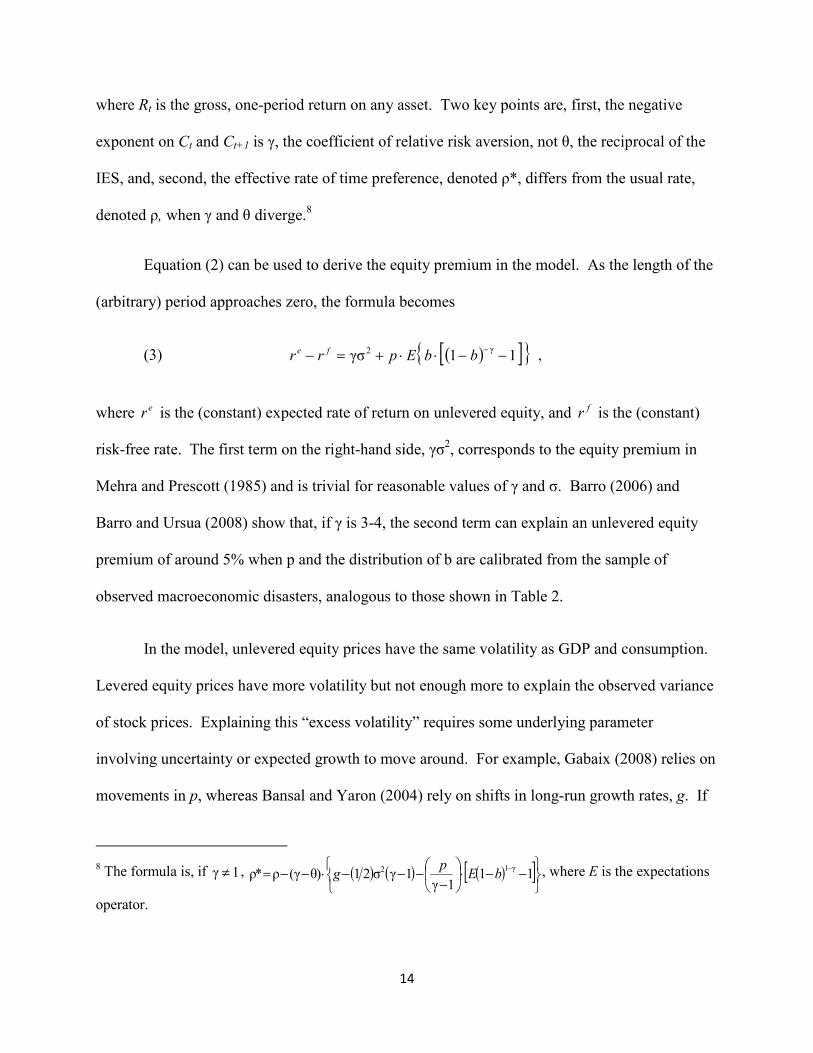
Equation (2) can be used to derive the equity premium in the model. As the length of the

(arbitrary) period approaches zero, the formula becomes

(3) ( )[ ]{ } 11γσγ2 −−⋅⋅+=− −

bbEprr fe ,

where er is the (constant) expected rate of return on unlevered equity, and fr is the (constant)

risk-free rate. The first term on the right-hand side, γσ2, corresponds to the equity premium in

Mehra and Prescott (1985) and is trivial for reasonable values of γ and σ. Barro (2006) and

Barro and Ursua (2008) show that, if γ is 3-4, the second term can explain an unlevered equity

premium of around 5% when p and the distribution of b are calibrated from the sample of

observed macroeconomic disasters, analogous to those shown in Table 2.

In the model, unlevered equity prices have the same volatility as GDP and consumption.

Levered equity prices have more volatility but not enough more to explain the observed variance

of stock prices. Explaining this “excess volatility” requires some underlying parameter

involving uncertainty or expected growth to move around. For example, Gabaix (2008) relies on

movements in p, whereas Bansal and Yaron (2004) rely on shifts in long-run growth rates, g. If

8 The formula is, if 1γ ≠ , ( ) ( ) ( )[ ]

−−⋅

−

−−−⋅−−= −11

1γ1γσ21)θγ(ρ*ρ

γ12 bEp

g , where E is the expectations

operator.

15

these shifts are temporary and orthogonal to contemporaneous consumption, the model’s

implications for the average equity premium do not change a lot from the formula in

equation (3). Thus, this extended framework may explain the average equity premium along

with the high volatility of stock prices.

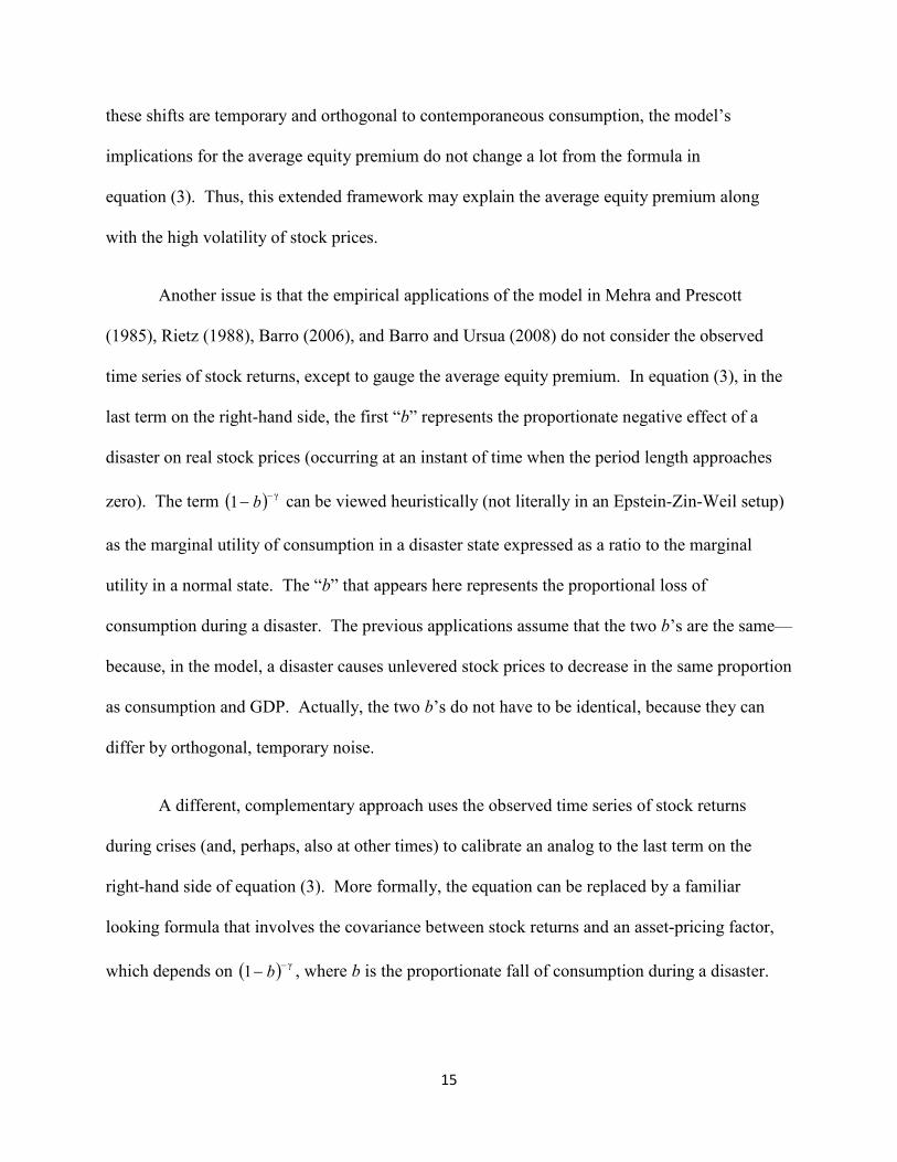
Another issue is that the empirical applications of the model in Mehra and Prescott

(1985), Rietz (1988), Barro (2006), and Barro and Ursua (2008) do not consider the observed

time series of stock returns, except to gauge the average equity premium. In equation (3), in the

last term on the right-hand side, the first “b” represents the proportionate negative effect of a

disaster on real stock prices (occurring at an instant of time when the period length approaches

zero). The term ( ) γ1

−− b can be viewed heuristically (not literally in an Epstein-Zin-Weil setup)

as the marginal utility of consumption in a disaster state expressed as a ratio to the marginal

utility in a normal state. The “b” that appears here represents the proportional loss of

consumption during a disaster. The previous applications assume that the two b’s are the same—

because, in the model, a disaster causes unlevered stock prices to decrease in the same proportion

as consumption and GDP. Actually, the two b’s do not have to be identical, because they can

differ by orthogonal, temporary noise.

A different, complementary approach uses the observed time series of stock returns

during crises (and, perhaps, also at other times) to calibrate an analog to the last term on the

right-hand side of equation (3). More formally, the equation can be replaced by a familiar

looking formula that involves the covariance between stock returns and an asset-pricing factor,

which depends on ( ) γ1

−− b , where b is the proportionate fall of consumption during a disaster.

16

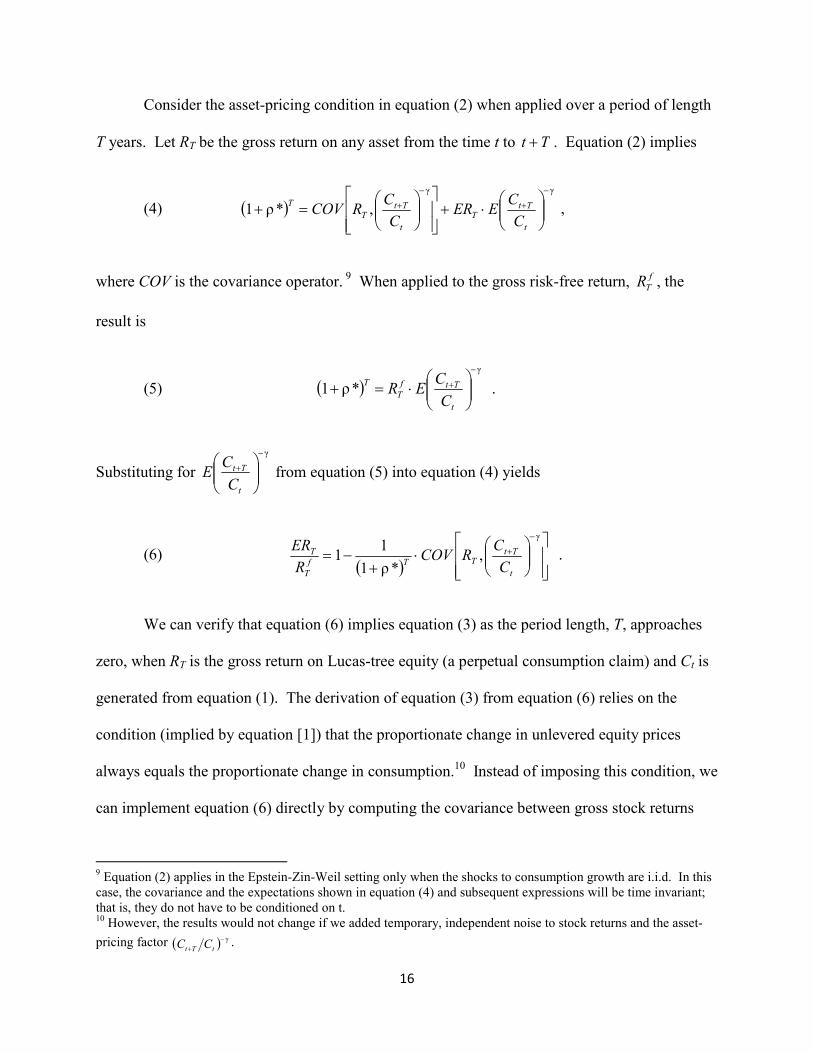
Consider the asset-pricing condition in equation (2) when applied over a period of length

T years. Let RT be the gross return on any asset from the time t to Tt + . Equation (2) implies

(4) ( )γγ

,*ρ1

−

+

−

+

⋅+

=+

t

TtT

t

TtT

T

C

CEER

C

CRCOV ,

where COV is the covariance operator. 9

When applied to the gross risk-free return, f

TR , the

result is

(5) ( )γ

*ρ1

−

+

⋅=+

t

Ttf

T

T

C

CER .

Substituting for

γ−

+

t

Tt

C

CE from equation (5) into equation (4) yields

(6) ( )

⋅

+−=

−

+

γ

,*ρ1

11

t

TtTTf

T

T

C

CRCOV

R

ER .

We can verify that equation (6) implies equation (3) as the period length, T, approaches

zero, when RT is the gross return on Lucas-tree equity (a perpetual consumption claim) and Ct is

generated from equation (1). The derivation of equation (3) from equation (6) relies on the

condition (implied by equation [1]) that the proportionate change in unlevered equity prices

always equals the proportionate change in consumption.10

Instead of imposing this condition, we

can implement equation (6) directly by computing the covariance between gross stock returns

9 Equation (2) applies in the Epstein-Zin-Weil setting only when the shocks to consumption growth are i.i.d. In this

case, the covariance and the expectations shown in equation (4) and subsequent expressions will be time invariant;

that is, they do not have to be conditioned on t. 10

However, the results would not change if we added temporary, independent noise to stock returns and the asset-

pricing factor ( ) γ−+ tTt CC .

17

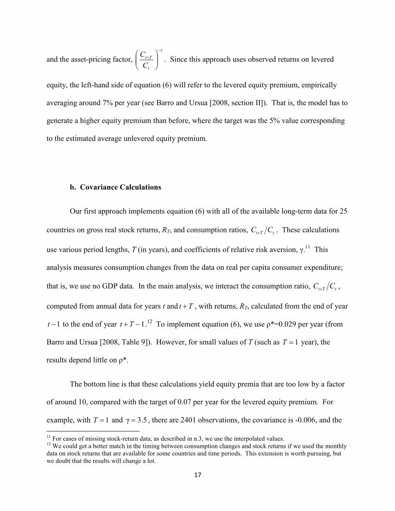
and the asset-pricing factor,

γ−

+

t

Tt

C

C. Since this approach uses observed returns on levered

equity, the left-hand side of equation (6) will refer to the levered equity premium, empirically

averaging around 7% per year (see Barro and Ursua [2008, section II]). That is, the model has to

generate a higher equity premium than before, where the target was the 5% value corresponding

to the estimated average unlevered equity premium.

b. Covariance Calculations

Our first approach implements equation (6) with all of the available long-term data for 25

countries on gross real stock returns, RT, and consumption ratios, tTt CC + . These calculations

use various period lengths, T (in years), and coefficients of relative risk aversion, γ.11

This

analysis measures consumption changes from the data on real per capita consumer expenditure;

that is, we use no GDP data. In the main analysis, we interact the consumption ratio, tTt CC + ,

computed from annual data for years t and Tt + , with returns, RT, calculated from the end of year

1−t to the end of year 1−+Tt .12

To implement equation (6), we use ρ*=0.029 per year (from

Barro and Ursua [2008, Table 9]). However, for small values of T (such as 1=T year), the

results depend little on ρ*.

The bottom line is that these calculations yield equity premia that are too low by a factor

of around 10, compared with the target of 0.07 per year for the levered equity premium. For

example, with 1=T and 5.3γ = , there are 2401 observations, the covariance is -0.006, and the

11

For cases of missing stock-return data, as described in n.3, we use the interpolated values. 12

We could get a better match in the timing between consumption changes and stock returns if we used the monthly

data on stock returns that are available for some countries and time periods. This extension is worth pursuing, but

we doubt that the results will change a lot.

18

equity premium is 0.006 per year. For 2=T and 5.3γ = , there are 2381 (overlapping)

observations, the covariance is -0.011, and the equity premium is 0.005 per year. If we shift the

timing to measure returns from the end of year t to the end of year Tt + or from the end of year

2−t to the end of year 2−+Tt , the computed equity premia are even smaller.

We know from Barro and Ursua (2008, Tables 9 and 10) that the calibrated results for the

equity premium depend mostly on the cases of extreme macroeconomic contraction. These

events, with contractions of size 0.10 or more, are the ones shown in Table 2 (for the 25

countries that also have long-term data on stock returns). Examination of panel A, which has the

58 cases of paired stock-market crashes and depressions, suggests two key properties. First,

crashes and depressions usually arise as multi-year events—but this feature was already captured

in the covariance analysis by allowing for period lengths, T, that exceeded one year. Second, the

timing between the stock-market crashes and the depressions is irregular. That is, unlike our

covariance calculations, the matches do not always refer to the same timing, such as relating

consumption changes between year t and year Tt + to gross stock returns from the end of year

1−t to the end of year 1−+Tt .

A prototypical case is the United States during the Great Depression—the stock return is

-0.55 for 1929-31 (gross return of 0.45), and the macroeconomic contraction is 0.25 for 1929-33.

This pattern—with the strongly negative stock return applying slightly prior to or coincident with

the macro contraction—also applies to other cases in Table 2, panel A. Examples include

Denmark, Sweden, Switzerland, and the United Kingdom in World War II; Chile, France,

Germany, Mexico, and Spain during the Great Depression; Canada over the period of World

War I and the Great Influenza Epidemic; Norway, Sweden, and the United States during this

epidemic; Germany at the end of the hyperinflation in 1922-23; India during its 1947-48 conflict

19

with Pakistan; Chile in the 1970s; Chile, Mexico, and Peru in the 1980s; and Finland in the early

1990s.

Some cases that deviate from this prototypical pattern can be explained by measurement

issues. For example, the need to interpolate stock-return data for Mexico 1915-18, Belgium in

World Wars I and II, Portugal 1974-77, and Spain 1936-40 may explain the patterns in which the

negative stock returns appear to lag the macroeconomic declines.

Other cases are likely to be affected strongly by wartime controls on prices and other

variables. An extreme example is Germany during World War II, where the controls—on

consumer prices starting in 1936 and on stock prices starting in 1943—lapsed only in 1948.

Clearly, the measured real stock return for 1948, -0.89, is way too low, especially because the

controls prevented the posted nominal stock prices from falling earlier. Correspondingly, during

the war and through 1947, the underestimation of true inflation and the propping up of reported

stock prices must have led to a substantial overstatement of real returns. These considerations

likely explain why the real stock return of -0.91 shown for 1944-48 in Table 2, panel A appears

to lag the macro decline of 0.41 for 1939-45. Moreover, an important point is that longer-term

real returns that bridge the controls are likely to be satisfactory. For example, the measured,

cumulative real stock return in Germany for 1939-48 of -0.85 is probably an accurate long-term

indicator.

Analogous effects from price controls likely arise for France and other countries during

World War II and, perhaps also, World War I.13

For France (also affected by missing data for

13

For the United States, in a case not included in Table 2, the measured real stock return of -0.25 for 1946-47 is

likely to be far below the “true” value because of the unwinding of price controls from 1945 to 1948. Barro (1978,

Table 2) estimates that the “true” price level was 53% above the reported value in 1945, 21% above in 1946, and 8%

20

1940-41), the cumulative real return for 1939-47 is -0.41. This long-term return, which bridges

the missing data and the likely price controls, is probably reliable. In contrast, there is an

apparent mismatch in timing between the reported real stock return of -0.69 shown for 1943-45

in Table 2, panel A and the macro contraction of 0.58 for 1938-43. Again, measurement

problems may explain the mismatch.

These considerations suggest that an alternative way to evaluate the formula for the

equity premium in equation (6) is to focus on the 58 cases of paired stock-market crashes and

depressions (Table 2, panel A) and to calculate the covariance in a flexible way that allows for

different timing for each case. Essentially, we compute the cross product between the demeaned

values of the stock returns shown in column 3 and the macro contractions shown in column 5.14

Then, in applying the result to equation (6), we measure the period length, T, as the average

duration (5.2 years) for the 58 paired cases. Subsequently, we go further by bringing into the

calculation the additional 163 cases that had either a stock-market crash or a depression but not

both (of which 137 had a stock-market crash and 26—those shown in Table 2, panel B—had a

depression).

In the first application of the method, we begin by computing the covariance for the 58

paired cases shown in Table 2, panel A. To carry out this calculation, we use the values shown

in columns 3 and 5 to express each gross stock return (one plus the rate of return) and

transformed consumption ratio,

γ−

+

t

Tt

C

C, as a deviation from the respective overall sample

above in 1947. Conversely, during the war, the controls led to an understatement of inflation and, hence, to an

overestimate of real stock returns. 14

In these calculations, we did not adjust for price controls, such as in Germany and France, by measuring real stock

returns over even longer periods than those shown in Table 2, panel A. Such adjustments, in conjunction with a

systematic analysis of price controls, might improve the results.

21

mean.15

(We use values of γ equal to 3, 3.5, and 4.) Then we add up the cross terms and divide

by the number of cases, 58, to compute the sample covariance. To get the contribution to the

overall covariance, we multiply by the weight applicable to the matched sample. This weight is

the ratio of the years in the 58-case sample (299, corresponding to an average duration of

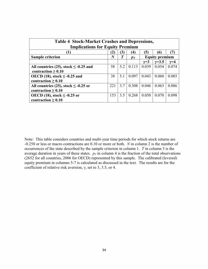
2.5=T years) to the total sample years (2652)—the result is 113.0=Tp , shown in the first line

of Table 4. To calculate the term on the right-hand side of equation (6), we multiply 0.113 by

the 58-case covariance and then divide by ( )T*ρ1+ , using 029.0*ρ = per year, as before, and

2.5=T years. Using 2.5=T again on the left-hand side of equation (6), we then compute the

equity premium, expressed per year.

The results for the three assumed values of γ are shown on the first line of Table 4. The

computed levered equity premium is 0.039 per year when 3γ = , 0.054 when 5.3γ = , and 0.074

when 4γ = . Thus, the model accords with the observed average levered equity premium of 0.07

if 4γ = . Note that this match relies only on the behavior during the 58 matched stock-market

crashes and depressions. Implicitly, the contribution to the covariance from the other 2353 years

in the sample is taken to be roughly zero.

The second line of Table 4 repeats the calculations for a sample limited to the 18 OECD

countries (which have a total of 2006 observations). The computed equity premia are somewhat

larger than those from the full sample—0.043 when 3γ = , 0.060 when 5.3γ = , and 0.085 when

4γ = . Although the weight, 097.0=Tp , is smaller for the OECD than for the overall sample,

the OECD also has a higher frequency of very large macroeconomic contractions. This last

consideration turns out to dominate and leads, thereby, to a higher equity premium for the OECD

15

For example, for the United States 1929-31, the gross real stock return of 0.45 is taken as a deviation from the

overall sample mean for all 25 countries of gross real stock returns over 3-year periods, which is 1.28.

22

than for the full sample. For the OECD, a value of γ close to 3.5 is adequate for roughly

matching the observed average levered equity premium of 0.07.

Lines 3 and 4 of Table 4 carry out the analysis for the larger sample of events that

includes stock-market crashes without depressions and depressions without stock-market

crashes. Thus, there are now 221 events for 25 countries and 153 events for 18 OECD countries.

The fraction, Tp , of the overall sample years contained in these sub-samples is much larger than

before—0.31 for the 25 countries and 0.27 for the OECD. However, since the covariance

between stock returns and macro contractions is not so high in the newly added group (because

these events were selected not to have pairings of stock-market crashes with depressions), the

incremental contribution to the computed equity premium is positive but modest in size. For the

full group of countries, the equity premium is now 0.046 at 3γ = , 0.063 at 5.3γ = , and 0.086 at

4γ = . For the OECD, the results are 0.050 at 3γ = , 0.070 at 5.3γ = , and 0.098 at 4γ = . Thus,

5.3γ = is now more clearly adequate to match the target value of 0.07.

Another 69% of the sample years for the 25 countries (73% for the OECD) are contained

neither in a stock-market crash nor a depression. We have not studied in detail the contribution

of this part of the sample to the computed equity premium. However, we can get an idea of the

effect by calculating the covariance between the one-year stock returns and the asset-pricing

factors, ( ) γ

1

−+ tt CC . That is, we use our initial approach for computing the covariance but look

here only at the years not contained within a stock-market crash or a depression. The result

when 5.3γ = is that the covariance is -0.005 for this sample when applied to 25 countries and

-0.003 for the 18 OECD countries. Weighting by the fraction of the overall years in the sample

(0.69 for the overall group and 0.73 for the OECD) implies that the incremental contribution to

23

the equity premium is 0.003 for the overall group and 0.002 for the OECD. Thus, by these

calculations, the inclusion of the rest of the sample years in the analysis has a slightly positive

impact on the equity premia reported in Table 4.

The bottom line is that a “flexible covariance analysis” applied to the asset-pricing

formula in equation (6) generates a reasonable levered equity premium if the coefficient of

relative risk aversion, γ, is around 3.5. The main element in this computation is the flexible

interpretation of the timing between stock-market crashes and depressions during the small

number of paired, multi-year events (58 in our sample).

This conclusion accords with the one reached by Barro and Ursua (2008, Tables 9

and 10), who followed Mehra and Prescott (1985) by considering only the sizes of

macroeconomic contractions and not the covariance with stock returns. This previous analysis

looked at multi-year depressions but did not require measurement of the timing between

depressions and stock-market crashes. In other words, the assumption that prices of unlevered

equity claims move in the same proportion as consumption (aside from temporary orthogonal

noise) substitutes for the complexities associated with matching the timing of stock returns and

consumption changes.

A key point is that the covariance calculation that “works” for the equity premium relies

almost entirely on the roughly 11% of the time-series observations that apply to matched stock-

market crashes and depressions (Table 2, panel A). The inclusion of the additional 20% of the

observations that feature unmatched stock-market crashes and depressions has a minor effect

(Table 4), and the consideration of the remaining 69% of the data from “normal times” has

essentially a zero effect. We think that further refinement of the results should focus even more

24

on the 11% of the data that matters for the equity premium. In particular, we need to consider

further how to carry out a covariance analysis that allows for flexible timing between stock

returns and consumption changes. An important part of this analysis is to deal more

satisfactorily with periods of missing annual data and with the price controls that characterize

many of the wartime observations.

IV. Conclusions and Future Research

The long-term history for 25 countries indicates that stock-market crashes (cumulative

real returns of -0.25 or worse) have substantial predictive power for depressions (cumulative

macroeconomic declines by 10% or more). For example, in a non-war environment, the

realization of a stock-market crash implies that the probability of a minor depression (fall in real

per capita consumer expenditure and GDP by 10% or more) is 20%, and the probability of a

major depression (decline by 25% or more) is 3%. Given the stock-market crashes for the

United States and other countries in 2008, these probabilities apply to 2008-09 and subsequent

years. In future research, we will consider whether the predictive content of stock-market

crashes for depressions can be improved by bringing in additional variables, such as the state of

the housing market.

The long-term data also show that the majority (64%) of minor, non-war depressions are

accompanied by stock-market crashes, whereas most major, non-war depressions (83%) are

accompanied by these crashes. Therefore, in the absence of a stock-market crash, the occurrence

of a depression is highly unlikely.

25

The full history of 2652 annual observations reveals 58 matched cases of stock-market

crashes and depressions, of which 45% are associated with war. The years contained in the 58

cases constitute 11% of the overall sample (because the average duration of a crisis was 5.2

years). The co-movement between stock returns and macroeconomic changes for the 58 cases

may be sufficient to explain the observed equity premium of 7%, assuming that the coefficient of

relative risk aversion is around 4. The required coefficient falls to about 3.5 if we bring in the

additional 20% of the sample that features a stock-market crash or depression but not both. A

crucial aspect of this analysis is that the computed covariances use a flexible timing pattern

between stock returns and macroeconomic changes. In future research, we plan to consider this

flexible covariance analysis in more detail. Part of this research involves the roles of missing

data and wartime price controls, which can distort the covariances calculated from a rigid timing

structure.

26

References

Bansal, R. and A. Yaron (2004). “Risks for the Long Run: A Potential Resolution of Asset-

Pricing Puzzles,” Journal of Finance, 59, August, 1481-1509.

Barro, R.J. (1978). “Unanticipated Money, Output, and the Price Level in the United States,”

Journal of Political Economy, 86, August, 549-580.

Barro, R.J. (2006). “Rare Disasters and Asset Markets in the Twentieth Century,” Quarterly

Journal of Economics, 121, August, 823-866.

Barro, R.J. (2009). “Rare Disasters, Asset Prices, and Welfare Costs,” American Economic

Review, March.

Barro, R.J. and J.F. Ursua (2008). “Macroeconomic Crises since 1870,” Brookings Papers on

Economic Activity, Spring, 255-350.

Dimson, E., P. Marsh, and M. Staunton (2008). “The Worldwide Equity Premium: A Smaller

Puzzle,” in R. Mehra, ed., Handbook of the Equity Risk Premium, Amsterdam, Elsevier.

Epstein, L.G. and S.E. Zin (1989). “Substitution, Risk Aversion, and the Temporal Behavior of

Consumption and Asset Returns: A Theoretical Framework,” Econometrica, 57, July, 937-969.

Fujino, S. and R. Akiyama (1977). Security Prices and Rates of Interest in Japan: 1874-1975,

Tokyo, Hitotsubashi University.

Gabaix, X. (2008). “Variable Rare Disasters: An Exactly Solved Framework for Ten Puzzles in

Macro-Finance,” National Bureau of Economic Research Working Paper 13724, January.

27

Haber, S., A. Razo, and N. Maurer (2003). The Politics of Property Rights: Political Instability,

Credible Commitments, and Economic Growth in Mexico, 1876-1929, New York, Cambridge

University Press.

Lucas, R.E. (1978). “Asset Prices in an Exchange Economy,” Econometrica, 46, November,

1429-1445.

Maddison, A. (2003). The World Economy: Historical Statistics, Paris, OECD (on the Internet

at www.ggdc.net/maddison).

Mehra, R. and E.C. Prescott (1985). “The Equity Premium: A Puzzle,” Journal of Monetary

Economics, 15, March, 145-161.

Rietz, T.A. (1988). “The Equity Risk Premium: A Solution,” Journal of Monetary Economics,

22, July, 117-131.

Samuelson, P.A. (1966). “Science and Stocks,” Newsweek, September 19.

Sarkees, M. R. (2000). "The Correlates of War Data on War: An Update to 1997," Conflict

Management and Peace Science, 18/1, 123-144, accessed on the Internet at

http://www.correlatesofwar.org/Datasets.htm, version 3.0.

Taylor, B. (2005). “GFD Guide to Total Returns on Stocks, Bonds and Bills,” available on the

Internet from Global Financial Data at www.globalfindata.com.

Weil, P. (1990). “Nonexpected Utility in Macroeconomics,” Quarterly Journal of Economics,

105, February, 29-42.

28

Table 1 U.S. Stock-Market Crashes since 1869 (1) (2) (3) (4) (5) (6) (7) (8)

Stock

period

Stock

return (-)

C

period

C

contraction

GDP

period

GDP

contraction

Macro

period

Macro

contraction

1907-07 0.32 1906-08 0.04 1906-08 0.10 1906-08 0.07

1916-20 0.47 1917-21 0.16 1918-21 0.12 1917-21 0.16

1929-31 0.55 1929-33 0.21 1929-33 0.29 1929-33 0.25

1937-37 0.37 1937-38 0.02 1937-38 0.04 1937-38 0.03

1939-41 0.29 1941-42 0.03 1939-40 -0.08 1941-42 0.03

1973-74 0.49 1973-74 0.02 1973-75 0.03 1973-75 0.02

2000-02 0.42 2000-01 -0.01 2000-01 0.00 2000-01 -0.01

2008-08 0.37 ? ? ? ? ? ?

Notes: Underlying stock returns are real rates of return (arithmetic) from end of previous year to

end of current year. Stock return in column 2 is cumulated real return (all negative) over period

shown in column 1. For example, 1929-31 refers to the cumulated return from the end of 1928

to the end of 1931. The cases selected are those with returns ≤ -0.250. C in columns 3 and 4 is

real per capita consumer expenditure. Contraction in column 4 is cumulated fractional decline

over period shown in column 3. For example, 1929-33 refers to the ratio of consumer

expenditure in 1933 (annual average) to that in 1929 (annual average). GDP is real per capita

GDP. Contraction in column 6 is cumulated fractional decline over period shown in column 5.

Macro contraction in column 8 is the average for C and GDP for non-war cases and C value for

wars and war aftermaths. The macro period in column 7 is the overlap for C and GDP when the

macro contraction is the average for C and GDP. When only C is used, the macro period

corresponds to that for C. For the United States, there are no other macroeconomic contractions

of size 0.10 or more. (1913-14 has a GDP contraction of 0.10 but a C contraction of only 0.05—

the stock return for 1913-14 is -0.16.)

29

Table 2 Depressions with and without Stock-Market Crashes

(25 countries with long-term data on stock returns and macro aggregates)

Panel A: Stock-Market Crashes and Depressions (58) (1) (2) (3) (4) (5)

Country Stock-Market

Period

Stock Return

(negative)

Macro

Period

Macro

Contraction

Australia 1929-30 0.25 1926-32 0.23

Belgium 1914-18* 0.76 1913-18 0.46

1929-31 0.48 1930-34 0.10

1937-39 0.26 1937-42 0.53

1942-48* 0.74 1942-46 0.13

Canada 1916-20 0.27 1918-21 0.20

1929-32 0.54 1928-33 0.29

Denmark 1917-17 0.27 1914-18 0.12

1919-22 0.60 1919-21 0.24

1937-40 0.27 1939-41 0.26

Finland 1989-91 0.47 1989-93 0.13

France 1913-20 0.62 1912-18 0.25

1929-31 0.46 1929-35 0.12

1943-45 0.69 1938-43 0.58

Germany 1914-20 0.91 1912-18 0.42

1922-22 0.63 1922-23 0.13

1929-31 0.52 1928-32 0.20

1944-48 0.91 1939-45 0.41

Italy 1944-45 0.89 1939-45 0.35

Japan 1897-98 0.54 1899-06 0.12

1943-47 0.97 1937-45 0.64

Netherlands 1918-22 0.47 1912-18 0.44

1944-46* 0.42 1939-44 0.54

Norway 1917-18 0.36 1916-18 0.17

1919-21 0.55 1919-21 0.16

Portugal 1974-78* 0.97 1974-76 0.10

Spain 1929-31 0.53 1929-33 0.10

1935-40* 0.43 1935-37 0.46

1935-40* 0.43 1940-45 0.14

Sweden 1917-18 0.60 1913-18 0.13

1919-20 0.30 1920-21 0.13

1939-40 0.26 1939-45 0.14

Switzerland 1914-20* 0.68 1912-18 0.15

1939-40 0.28 1939-45 0.15

United Kingdom 1912-20 0.60 1915-18 0.17

1937-40 0.41 1938-43 0.17

30

(1) (2) (3) (4) (5)

United States 1916-20 0.47 1917-21 0.16

1929-31 0.55 1929-33 0.25

Chile 1929-31 0.40 1929-32 0.37

1972-72 0.27 1972-76 0.40

1981-84 0.56 1981-85 0.25

Colombia 1931-31 0.28 1929-32 0.11

India 1940-42 0.30 1937-42 0.13

1940-42 0.30 1943-46 0.13

1946-49 0.49 1947-50 0.18

Mexico 1909-18* 0.79 1909-16 0.25

1924-31 0.55 1926-32 0.31

1980-82 0.81 1981-88 0.14

1994-96 0.38 1994-95 0.10

Peru 1967-76 0.66 1975-79 0.14

1981-82 0.86 1981-83 0.11

1987-88 0.76 1987-92 0.31

Venezuela 1946-47 0.28 1948-52 0.14

1958-61 0.34 1957-64 0.19

1977-81 0.65 1977-86 0.28

1988-89 0.70 1988-89 0.10

1992-95 0.55 1992-99 0.11

1997-2001 0.60 2001-03 0.16

Panel B: Depressions without Stock-Market Crashes (26)

(1) (2) (3) (4) (5)

Country Stock-Market

Period

Stock Return

(negative)

Macro

Period

Macro

Contraction

Australia 1889-89 0.02 1889-95 0.27

1915-15 0.16 1913-18 0.24

1940-41 0.09 1938-44 0.30

Canada 1907-07 0.09 1906-08 0.10

1913-14 0.18 1912-15 0.13

Denmark 1947-48 0.07 1946-48 0.14

Finland 1928-29 0.12 1928-32 0.13

1939-39 0.05 1938-42 0.24

France 1871-71 0.12 1864-71 0.16

1882-85 0.13 1882-86 0.11

New Zealand 1930-31 0.13 1929-32 0.18

1940-40 0.01 1939-44 0.22

Norway 1939-40 0.05 1939-44 0.15

31

(1) (2) (3) (4) (5)

Portugal 1936-36 -0.03 1934-36 0.13

1937-40 0.22 1939-42 0.10

Spain 1896-96 0.07 1892-96 0.15

Chile 1913-15 0.08 1911-15 0.21

1920-20 0.05 1918-22 0.15

Colombia 1940-41 0.03 1939-43 0.14

Mexico 1920-20 0.12 1921-24 0.12

Peru 1930-32 0.18 1929-32 0.20

South Africa 1914-15 0.08 1912-17 0.23

1931-32 0.15 1928-32 0.12

1981-81 0.12 1981-87 0.10

Venezuela 1932-32** 0.04 1930-33 0.24

1942-42 0.03 1939-42 0.11

*These periods include interpolated stock returns.

**Data missing before 1930.

Notes: See notes to Table 1 on measures of stock returns and macroeconomic contractions.

Panel A shows the 58 paired cases with stock-market crashes (cumulative returns of -0.250 or

less) and depressions (macroeconomic contractions of 0.10 or more). Panel B shows the 26

cases of macro contractions not accompanied by stock-market crashes. Not shown are 137 cases

with stock-market crashes unaccompanied by depressions. Bold for macro period indicates

wartime interval (limited to active combatants).

For cases of missing data on consumer expenditure, C, macro contractions were based on GDP

except for war aftermaths (which were left as missing data) and during wars when the indicated

GDP fall was less than 0.10 (also left as missing data). For wartime contractions, when C and

GDP data were available, the macro contraction was based on C when this decline was greater

than that in GDP. When the GDP decline was larger, the macro contraction was computed as the

average of the C and GDP contractions. Annual data on stock returns were missing (typically

because of closed markets) for Belgium 1914-18 and 1944-46, Mexico 1915-18, Netherlands

1944-46, Spain 1936-40, Portugal 1974-77, and Switzerland 1914-16. The stock returns that

include these periods were based on cumulative, multi-year returns over periods that bridged the

gaps in the annual data.

32

Table 3 Frequencies of Stock-Market Crashes and Depressions

Part A: Non-War and War Observations Combined Numbers of events

Stock

return ≤

Macro

Contraction ≥

Stock-Market

Crashes

Depressions Both

All countries (25) -0.25 0.10 195 84 58 (.30, .69)

-0.25 0.15 195 49 35 (.18, .71)

-0.25 0.20 195 34 25 (.13, .74)

-0.25 0.25 195 23 21 (.11, .91)

-0.25 0.30 195 15 14 (.07, .93)

-0.30 0.10 159 84 48 (.30, .57)

-0.30 0.15 159 49 29 (.18, .59)

-0.30 0.20 159 34 20 (.13, .59)

-0.30 0.25 159 23 18 (.11, .78)

-0.30 0.30 159 15 12 (.08, .80)

OECD countries (18) -0.25 0.10 137 54 38 (.28, .70)

-0.25 0.15 137 34 25 (.18, .74)

-0.25 0.20 137 23 18 (.13, .78)

-0.25 0.25 137 16 14 (.10, .88)

-0.25 0.30 137 11 10 (.07, .91)

-0.30 0.10 111 54 31 (.28, .57)

-0.30 0.15 111 34 20 (.18, .59)

-0.30 0.20 111 23 14 (.13, .61)

-0.30 0.25 111 16 12 (.11, .75)

-0.30 0.30 111 11 9 (.08, .82)

33

Part B: Non-War and War Observations Compared Numbers of Events

Non-war only War only

(1) (2) (3) (4) (5) (6) (7) (8)

Stock

≤

Macro

≥

Stock

Depression Both Stock

Depression Both

All countries (25) -0.25 0.10 158 50 32 (.20, .64) 37 34 26 (.70, .76)

-0.25 0.15 158 22 15 (.09, .68) 37 27 20 (.54, .74)

-0.25 0.20 158 13 9 (.06, .69) 37 21 16 (.43, .76)

-0.25 0.25 158 6 5 (.03, .83) 37 17 16 (.43, .94)

-0.25 0.30 158 1 1 (.01, 1.00) 37 14 13 (.35, .93)

-0.30 0.10 130 50 26 (.20, .52) 29 34 22 (.76, .65)

-0.30 0.15 130 22 12 (.09, .55) 29 27 17 (.59, .63)

-0.30 0.20 130 13 7 (.05, .54) 29 21 13 (.45, .62)

-0.30 0.25 130 6 5 (.04, .83) 29 17 13 (.45, .76)

-0.30 0.30 130 1 1 (.01, 1.00) 29 14 11 (.38, .79)

OECD countries (18)

-0.25 0.10 109 28 19 (.17, .68) 28 26 19 (.68, .73)

-0.25 0.15 109 13 10 (.09, .77) 28 21 15 (.54, .71)

-0.25 0.20 109 7 6 (.06, .86) 28 16 12 (.43, .75)

-0.25 0.25 109 3 2 (.02, .67) 28 13 12 (.43, .92)

-0.25 0.30 109 0 0 (.00, --) 28 11 10 (.36, .91)

-0.30 0.10 90 28 15 (.17, .54) 21 26 16 (.76, .62)

-0.30 0.15 90 13 7 (.08, .54) 21 21 13 (.62, .62)

-0.30 0.20 90 7 4 (.04, .57) 21 16 10 (.48, .63)

-0.30 0.25 90 3 2 (.02, .67) 21 13 10 (.48, .77)

-0.30 0.30 90 0 0 (.00, --) 21 11 9 (.43, .82)

Part A combines non-war and war events. Part B considers non-war and war events separately

(where “war” indicates that the period of macroeconomic contraction overlaps with active

combat status in a major inter-state or intra-state conflict). The numbers of events refer to stock-

market returns ≤ the amount shown or macro contractions ≥ the amount shown or both. In the

last column of part A and columns 5 and 8 of part B, the fractions in parentheses are, first, the

frequency of contractions ≥ the amount shown, given that the stock return is ≤ the amount

shown, and, second, the frequency of stock returns ≤ the amount shown, given that the

contraction is ≥ the amount shown.

34

Note: This table considers countries and multi-year time periods for which stock returns are

-0.250 or less or macro contractions are 0.10 or more or both. N in column 2 is the number of

occurrences of the state described by the sample criterion in column 1. T in column 3 is the

average duration in years of these states. pT in column 4 is the fraction of the total observations

(2652 for all countries, 2006 for OECD) represented by this sample. The calibrated (levered)

equity premium in columns 5-7 is calculated as discussed in the text. The results are for the

coefficient of relative risk aversion, γ, set to 3, 3.5, or 4.

Table 4 Stock-Market Crashes and Depressions,

Implications for Equity Premium

(1) (2) (3) (4) (5) (6) (7)

Sample criterion N T pT Equity premium

γ=3 γ=3.5 γ=4

All countries (25), stock ≤ -0.25 and

contraction ≥ 0.10

58 5.2 0.113 0.039 0.054 0.074

OECD (18), stock ≤ -0.25 and

contraction ≥ 0.10

38 5.1 0.097 0.043 0.060 0.085

All countries (25), stock ≤ -0.25 or

contraction ≥ 0.10

221 3.7 0.308 0.046 0.063 0.086

OECD (18), stock ≤ -0.25 or

contraction ≥ 0.10

153 3.5 0.268 0.050 0.070 0.098