NATURAL RELEASES OF

CO2: BUILDING

KNOWLEDGE FOR CO2

STORAGE

ENVIRONMENTAL

IMPACT ASSESSMENTS

Report: 2011-03

June 2011

INTERNATIONAL ENERGY AGENCY

The International Energy Agency (IEA) was established in 1974 within the framework of the Organisation for Economic Co-operation and Development (OECD) to implement an international energy programme. The IEA fosters co-operation amongst its 28 member countries and the European Commission, and with the other countries, in order to increase energy security by improved efficiency of energy use, development of alternative energy sources and research, development and demonstration on matters of energy supply and use. This is achieved through a series of collaborative activities, organised under more than 40 Implementing Agreements. These agreements cover more than 200 individual items of research, development and demonstration. IEAGHG is one of these Implementing Agreements.

DISCLAIMER AND ACKNOWLEDGEMENTS

This report was prepared by Dr Ameena Camps of IEAGHG as a record of the events of the workshop. The IEAGHG workshop on Natural Releases of CO2: Building Knowledge for CO2 Storage Environmental Impact Assessments was organised by IEAGHG in co-operation with CO2GeoNet and Bundesanstalt für Geowissenschaften und Rohstoffe (BGR). The organisers acknowledge the financial support provided by IPAC-CO2 Research Inc. for this meeting and the hospitality provided by the hosts, BGR, at the See Hotel, Maria Laach, Germany. A steering committee guides the direction of this network. The steering committee members were: • Tim Dixon, IEAGHG (Chair) • Ameena Camps, IEAGHG (Co-Chair) • Franz May, BGR (Host) • Salvatore Lombardi, ‘La Sapienza’ University of Rome • Travis McLing, Idaho National Laboratory • Jonathan Pearce, British Geological Survey (BGS) • Katherine Romanak, Gulf Coast Carbon Centre, The University of Texas at Austin • Lee Spangler, Montana State University

The International Steering Committee also wish to acknowledge Heike Rütters of BGR; Julia West of the British Geological Survey, and Samantha Neades of IEAGHG.

COPYRIGHT AND CITATIONS Copyright © IEA Environmental Projects Ltd. (IEAGHG) 2011. All rights reserved. The report should be cited in literature as follows: ‘IEAGHG, “Summary report of the IEAGHG Workshop on Natural Releases of CO2: Building Knowledge for CO2 Storage Environmental Impact Assessments”, June 2011’ Further information or copies of the report can be obtained by contacting IEAGHG at: IEAGHG, Orchard Business Centre, Stoke Orchard, Cheltenham, GLOS., GL52 7RZ, UK Tel: +44(0) 1242 680753 Fax: +44 (0)1242 680758 E-mail: mail@ieaghg.org Internet: www.ieaghg.org

1

Summary Report of the IEAGHG Workshop -

Natural Releases of CO2: Building Knowledge for CO2 Storage Environmental Impact Assessments

2nd – 3rd November 2010 Maria Laach, Germany

Organised by IEAGHG

Hosted by CO2GeoNet and BGR

With the sponsorship of:

IEAGHG

and the:

International Performance Assessment Centre for Geological Storage of CO2 (IPAC-CO2)

2

IEAGHG WORKSHOP ON NATURAL RELEASES OF CO2: BUILDING KNOWLEDGE FOR CO2 STORAGE ENVIRONMENTAL IMPACT

ASSESSMENTS

Executive Summary The IEAGHG workshop on Natural Releases of CO2: Building Knowledge for CO2 Storage Environmental Impact Assessments was held in Maria Laach, Germany, in November 2010 and hosted by CO2GeoNet and BGR. The workshop was well attended, with forty seven participants from over ten different countries.

Sessions included: Setting the Scene; Releases, Magnitudes and Impacts: Marine Environments and Terrestrial Environments; Mobilisation of Brine and Metals; Near Surface vs. Deep Subsurface Mechanisms and, Monitoring Challenges in Light of Natural Systems. Due to considerable interest in the workshop and an overly prescribed agenda, poster sessions were included within coffee and lunch breaks, with eight presented posters during the workshop.

Presentations showed there are now regulations in place specifying the need to monitor and detect leakage and impacts, both in the EU CCS Directive to detect and measure impact, and in the ETS Directive to quantify leakage; however uncertainty remains and the research community are asked to provide information to move this forward. There have been various studies on natural and controlled release sites, which can be used to learn where CO2 leakage is more likely to occur; the structural or geological controls on leakage should any occur; potential rates; spatial-temporal scale and transport processes; how humans, plants and animals are impacted; mitigation strategies and, the most cost effective design of monitoring techniques. Though much can be learnt it was noted it is important to recognise limitations as well as the benefits and maintain the context ensuring experimental programmes are created to understand key processes and responses to changing conditions.

Research to-date has shown decreased biodiversity in environments of enriched CO2, and changes in species (particularly calcareous organisms); however species can cope if there is sufficient energy from other sources e.g. methane. Particularly noteworthy was the presentation on mofettes by Hardy Pfanz, which showed CO2 terrestrial release sites can be mapped by plant and soil-animal species (introducing the terms ‘mofettophilic’ and ‘mofettophobic’), and concentrations may even be determined by understanding the impact on specific species, with research highlighting the possibility of global indicator species (see section 2.2.1).

A portfolio of technologies is recommended for detection, quantification and system understanding, and shallow monitoring strategies should be iterative based upon deep monitoring tools. There are various monitoring technologies available, and they are seen to be sufficient to detect CO2 bubbles streams and to monitor chemical effects (such as pH and pCO2) in the marine environment, including hydroacoustical methods; though technologies to assess impacts are still being developed or are currently being applied e.g. ROVs (see section 2.1). Various tools are required to determine the effects of CO2 injection and to ascertain what is being mobilised new sensors need to be developed and, existing sensors improved (see section 3). Additionally, there is a need for more site investigations to understand CO2 processes and their natural variability, as baseline monitoring is crucial to meet political and public perception challenges (see section 5). Research indicates it is important to monitor gases other than CO2, such as nitrogen and oxygen, to aid understanding of site-specific processes (see section 5.2.1), and in terms of microbiological impacts, there is a systematic response to high CO2 concentrations: understanding this response is critical to the implementation of CCS (see section 4).

A key presentation of the workshop was that from Elizabeth Keating, presenting on field, laboratory and modelling results from a natural analogue site near Chimayó New Mexico aiming to understand potential groundwater quality impacts (see section 3.1). From the collation of these approaches, it was evident the presence of trace metals was more closely associated with brackish water

3

displacement than in-situ mobilisation; hence rather than direct trace metal leaching, the intrusion of brackish water displaced by CO2 may be more important in relation to groundwater impacts; hence further research in this area is of extreme importance, and notes the importance of combined laboratory, field and modelling research.

It was clear from the quantity of experience and research results available from a variety of disciplines there must be a collated effort to draw together these results for much needed information on impacts and geological processes. For example a wealth of information is available from hydrothermal outcrop studies which show self-sealing secondary trapping through water-CO2-rock interactions (see section 4.1), and geological research indicating association with CO2 accumulations or releases and seismicity (see section 4.2) which remains to be a poorly understood research area in the CCS community: highlighting the importance of knowledge transfer from different research fields.

Final discussions highlighted several main knowledge gaps:

• Further understanding of impacts and processes of CO2 displaced waters.

• Further understanding of physical processes of CO2 flow in aquifers.

• A need to draw together studies to produce an indicator species database.

• A need for field studies to investigate potential mobilisation of brine and metals.

• A need for more data on long-term impacts of CO2.

• A need for more data on natural background CO2 in offshore environments.

• Further understanding of mechanisms in the deep subsurface, particularly in regard to understanding of caprocks, additional barriers and trapping mechanisms; drawing from research in other geological communities.

• There is a need to further understand the association of seismicity with natural accumulations of CO2.

Participants of the workshop recommend:

• A follow-up meeting given the amount of interest and the workshop establishment of a research community.

• An integrated, international, cross-disciplinary natural analogue/controlled release program given the wide spread of researchers who can impart knowledge to advance knowledge in this critical research area.

• Future and current research needs to integrate modelling, field studies and laboratory research.

• Further research on long-term impacts in marine and terrestrial environments.

• It is important to expand this community to include other areas of relevant research bringing together biologists, geologists and many other experts to advance knowledge, as has clearly happened at this workshop.

This highly productive and informative workshop expresses the importance of such meeting at a time when despite emerged CCS regulations requiring Environmental Impact Assessments uncertainties remain and the research community are asked to advance understanding.

4

Contents

EXECUTIVE SUMMARY ........................................................................................................................................ 2

CONTENTS ............................................................................................................................................................... 4

INTRODUCTION .....................................................................................................................................6

Welcome Session ................................................................................................................................................ 6

SESSION 1: SETTING THE SCENE ...................................................................................................8

1.1 Overview of Regulatory Requirements, Tim Dixon, IEAGHG .............................................................. 8 1.2 Overview from a North American Perspective, Travis McLing, Idaho National Laboratory and Lee

Spangler, Montana State University .................................................................................................... 9 1.3 Overview from an EU RISCS perspective, Dave Jones, BGS ............................................................. 11 1.4 What can we learn from natural releases of CO2, Jennifer Lewicki, Lawrence Berkeley National

Laboratory .......................................................................................................................................... 12 1.5 Discussion Session 1 ........................................................................................................................... 14

SESSION 2: RELEASES, MAGNITUDES AND IMPACTS ...........................................................17

2.1 Marine Environments ............................................................................................................................. 17

2.1.1 RITE’s research and development activity of marine environment assessment technology for CCS, Michimasa Magi, RITE ......................................................................................................... 17

2.1.2 Natural CO2 Seeps at the seabed, Klaus Wallman, IFM-GEOMAR .............................................. 18 2.1.3 Natural CO2-leaking marine sites off the coast of Italy - a resource for studying gas migration

processes, testing monitoring techniques, and examining potential impacts, Salvatore Lombardi, ‘La Sapienza’ University of Rome ................................................................................ 20

2.1.4 Study of a submarine CO2 natural-analogue by means of Scientific Diving techniques, Giorgio Caramanna, NCCCS-CICCS .......................................................................................................... 22

2.1.5 Discussion Session 2 ...................................................................................................................... 23

2.2 Terrestrial Environments .............................................................................................................. 25

2.2.1 Life in dry, terrestrial mofette areas, Hardy Pfanz, University of Duisberg-Essen ........................ 25 2.2.2 Ecosystem effects of high CO2 concentrations - A natural analogue study at the Laacher See,

Martin Krüger, BGR ....................................................................................................................... 26 2.2.3 Discussion Session 3 ...................................................................................................................... 28

SESSION 3: MOBILISATION OF BRINE AND METALS ..............................................................31

3.1 The challenge of predicting groundwater quality impacts in CO2 leakage scenarios: Results from field, laboratory, and modelling studies at a natural analogue site in New Mexico, USA, Elizabeth Keating, Los Alamos National Laboratory ......................................................................................... 31

3.2 Intrusion of CO2 and impurities in a freshwater aquifer – impact evaluation by reactive transport modelling, Chan Quang Vong, BRGM................................................................................................ 32

3.3 Monitoring of Substances Mobilised by CO2, Charles Jenkins CO2CRC and CSIRO; on behalf of Linda Stalker, CO2CRC and CSIRO .................................................................................................. 33

3.4 Discussion Session 4 ........................................................................................................................... 34

SESSION 4: NEAR SURFACE VS. DEEP SUBSURFACE MECHANISMS ..................................36

4.1 Outcrops and Escape Mechanisms, Lee Spangler, Montana State University on behalf of Dave Bowen, Montana State University ....................................................................................................... 36

4.2 Volcanic and non-Volcanic release of CO2 in Italy, Giovanni Chiodini, Istituto Nazionale di Geofisica e Vulcanologia .................................................................................................................... 38

4.3 Near surface interactions, Travis McLing, Idaho National Laboratory ............................................. 39 4.4 Tracking CO2 Movement, Rob Arts, TNO-NITG ................................................................................ 41 4.5 The effects of high CO2 concentrations on microbial communities at natural CO2 seeps and

depleted natural gas reservoirs, Janin Frerichs, BGR ....................................................................... 42

5

4.6 Discussion Session 5 ........................................................................................................................... 43

SESSION 5: MONITORING CHALLENGES IN LIGHT OF NATURAL SYSTEMS ..................45

5.1 Part I .................................................................................................................................................. 45

5.1.1 The challenge of underwater gas (leakage) monitoring, Ingo Moeller, BGR ................................ 45 5.1.2 An overview of monitoring requirements and technologies for offshore storage sites, Jonathan

Pearce, BGS ................................................................................................................................... 46 5.1.3 Overview of Monitoring Controlled Releases, Lee Spangler, Montana State University ............... 48 5.1.4 CO2 leakage quantification methods: advantages and limitations, Sevket Durucan, Imperial

College London .............................................................................................................................. 49

5.2 Part II ................................................................................................................................................ 50

5.2.1 Soil-gas behaviour and measurement in a carbon-reactive natural analogue; implications for near-surface monitoring, Katherine Romanak, The University of Texas Gulf Coast Carbon Center ............................................................................................................................................. 50

5.2.2 Otway Project Monitoring, Charles Jenkins, CO2CRC and CSIRO .............................................. 52 5.2.3 Regional and site-scale baseline surveys of near-surface gas geochemistry parameters -

understanding natural variability as a framework for monitoring programs and public acceptance, Salvatore Lombardi, ‘La Sapienza’ University of Rome ............................................ 54

5.2.4 Discussion Session 6 ...................................................................................................................... 55

SESSION 6: OUTCOMES AND RECOMMENDATIONS ...............................................................57

FIELD TRIP OVERVIEW ................................................................................................................................... 62

6

Introduction

Welcome Session

Chaired by Tim Dixon, IEAGHG and Franz May, CO2GeoNet/BGR

The meeting was opened by Tim Dixon of IEAGHG who welcomed all the participants to Laacher See of Maria Laach, thanking the hosts of the meeting – CO2GeoNet and BGR, and the sponsors – IPAC-CO2.

Tim followed his welcoming address by providing a brief overview of the IEA Greenhouse Gas R & D Programme, its members, its aims and objectives, networks and studies. Tim then presented the previous IEAGHG workshop, held in September 2008: Defining R & D needs to assess environmental impacts of potential leaks from CO2 storage, its key finding, conclusions and recommendations which included a recommendation for an additional workshop focussed on natural releases of CO2. He then provided the participants with the programme for the next two days, introducing and thanking the International Steering Committee.

Tim passed over to Franz May who welcomed participants to the Eifel region and provided an overview of Bundesanstalt für Geowissenschaften und Rohstoffe (BGR).

The Eifel region has many sites of natural CO2 releases, as well as manmade CO2. Many sources of CO2 are used for water production or other technical aspects, and people have learned to live with CO2.

BGR is a classical geological survey, forming in 1873 as the Royal Prussian Geological Survey founded in Berlin. After the war, Germany was divided, and a new geological survey was formed in Hannover in 1958. After unification, the two surveys were merged into the federal institute of BGR. We therefore have staff in Berlin and Hannover, but most of us are based in Hannover. BGR’s main role is to advise and inform the federal government. Within BGR there are four main divisions: Energy Resources and Mineral Resources, Groundwater and Soil Science, Underground Space for Storage and Economic Use, and Geoscientific Information, International Cooperation. An additional division has been added recently – Raw Materials Agency – as there has been large fluctuations in the cost of raw materials. Geological CO2 Storage fits into the third division of Underground Space for Storage and Economic Use.

Germany has to import much of its energy resources except natural gas, biomass, and some lignite, therefore energy resources is very important for the country and BGR is involved in frontier exploration as well as resource research. Groundwater is a strategic resource, and the majority of BGR’s work in Europe involved groundwater quality work, however elsewhere quality and availability issues are both important, for example in Afghanistan BGR’s work also involves finding water resources. The Government is responsible for the exploration of potential storage formations and sites repositories of high level radioactive waste in, and much of the geoscientific work has been assigned to BGR. We can learn a lot from radioactive waste disposal such as cap rock integrity and permeability. CO2 storage and geothermal energy are

7

hot topics for BGR, both under the same division. In terms of CO2 storage, BGR’s work involves advice to government, industry and the public, providing regulatory advice using the EC Directive, discussing with neighbouring countries especially as many storage sites proposed are cross-border sites, and international work with both developed and developing countries.

BGR is also a classical geological survey, and so also works on the collection and maintenance of geoscientific data and samples, e.g. the geological map of Europe 1:5 Mio, has a national seismological observatory, which is also responsible for monitoring of nuclear tests, according to the nuclear test ban treaty, and records infrasound waves transmitted through the atmosphere for the detection of tests. BGR’s Geo-Risks work involves analysis of potential geological risks such as earthquakes and flooding, and including research on the Laacher See volcano which should help to up-date the risk assessment for this site, which is generally assumed to be a safe place, in a historic, but not in a geo-historic time frame.

Franz closed his presentation on a photograph of Laacher See, wishing all participants a successful workshop and a pleasant stay in the Eifel, passing on to Rob Arts for a CO2GeoNet presentation.

Rob Arts began by introducing what CO2GeoNet is and how it formed from the EU Framework 6 proposal to the call for a European Network of Excellence, to the present day Association under French law.

CO2GeoNet is spread over 7 countries including Denmark, France, Germany, Italy, The Netherlands, Norway and the UK, integrating 13 research institutions and over 300 researchers. Activities include joint research, scientific advice, training, information and communication.

2009 was the year during which the network became an Association, with the end of the EC contract in March, and the start of Association activities in April. Management of the Association consists of the President, Nick Riley from the British Geological Survey, the Secretary General, Sergio Persoglia from OGS, and an Executive Committee which changes every year. Activities have included the co-organisation of the 1st IEAGHG CO2 storage modelling workshop, and joint research such as on the development of the Benthic Chamber lander. In terms of training and capacity building, CO2GeoNet have been involved in a number of activities such as professional training courses in New Orleans and including the OPEC-IEAGHG Summer School in Algeria and the CCOP Training course on CO2 storage in Bangkok. CO2GeoNet are also currently involved in the EAGE Student Lecture Tour 2010-2011, providing lectures to introduce CCS to more than 40 universities in Europe.

Rob Arts closed his presentation by highlighting the annual CO2GeoNet open forum, which this year took place in May in Venice, providing participants with contact information for enquiries.

8

Session 1: Setting the Scene Chaired by Rob Arts, TNO

1.1 Overview of Regulatory Requirements Tim Dixon, IEAGHG

Tim began by examining the context for environmental impacts of CO2 storage, introducing risk assessment requirements and the need for understanding of impacts.

There has been a lot of research to look at the strength of the CO2 storage system to minimise the chance of leakage, but it is also important to know if it was to leak, what would happen. There is therefore a need to be able to detect, remediate and to perform an impact assessment (and recovery assessment), both in the short-term (operational phase) and in the long term. Impacts can be local or global. In terms of global impact, there are also impacts on the ETS and greenhouse gas inventory which we won’t be looking at.

Tim went on to present the development of CO2 storage regulations on both a global and European level.

One of the first major activities in terms of regulatory developments was the global marine treaty of the London Convention and Protocol; which was found to be prohibiting some CO2 storage configurations. These prohibitions were removed in the amendment in 2007, and specific CO2 guidelines were issued. OSPAR, the marine treaty for the NE Atlantic, also prevented certain CCS configurations, and this was amended in 2007 though still requires ratification by at least 7 Contracting Parties. OSPAR also provides guidelines for Risk Assessment and Management of Storage of CO2 in Geological Formations which includes the Framework for Risk Assessment and Management (FRAM). The marine treaties basically provide EIA guidance, including exposure assessment, effects assessment and risk characterisation.

Modelled on the OSPAR guidelines and the amendment, and following the IPCC GHG guidelines, is the EU CCS Directive, enabling a regulatory framework to ensure environmentally sound CCS, with the objective of permanent storage. The Directive includes the requirement for an exploration and storage permit, and states a storage permit will only be issued if ‘no significant risk of leakage, and if no significant negative environmental or health impacts are likely to occur’. The Directive also includes the need for a corrective measures plan, an exposure assessment, effects assessment, and the need for baseline monitoring in a monitoring plan. It is not overly prescriptive. The effects assessment is based on the sensitivity to species, communities and habitats to identify potential leakage events, including the effects of other substances in the CO2 stream and at a range of temporal and spatial scales. The

9

Commission are assisting by producing guidance documents, providing more detail on the effects assessment in GD1.

CCS can already be included in the ETS in Phase II (2008-2012) by ‘opt-in’ but in Phase III from 2013, CCS will be fully included. For this the site and operation will need to comply with the CCS Directive, and there are new monitoring and reporting guidelines, stating any leakage will require the surrender of allowances. Therefore, there are regulations in place specifying the need to monitor to detect leakage and impacts, both in the CCS Directive to detect and measure impact, and in the ETS Directive to quantify leakage.

As the North American perspective follows this talk, this is an EU based presentation, but there are also Australian regulations which do not go into much detail on the EIA. A crucial word comes up in OSPAR and the CCS Directive – ‘significant’ – which is difficult to define. We are left with uncertainty, and the research community is asked to provide information to move this forward. The first projects will be very important to determine what level of detail is required. For the Gorgon project, very little is provided on EIA for CO2 storage, so Americans and the EU may provide the answer and lead the way.

Q. In reference to the ETS, are they asking for CO2 which escapes from the geological reservoir or that which enters drinking water – what is defined as leakage?

A. Leakage is strictly what moves outside of the storage formation, but for the ETS it is CO2 which escapes out of the water column or to the atmosphere.

1.2 Overview from a North American Perspective

Travis McLing, Idaho National Laboratory and Lee Spangler, Montana State University

CCS in the U.S. is a little different, and mid-term elections may change things. Before I would have said carbon cap and trade was imminent, but not today with the current recession and a change of focus in government. There are some things happening in the U.S., for example even in California there is a movement to set aside some of the emissions standards to get through the economic recession.

The majority of CCS developments seem to be in the Western U.S. as it is here where there is a Western energy corridor. In Canada we see a different picture, with both provincial and federal regulations progressing. Canada’s biggest trading route for energy happens to be the U.S., and so the Canadians are being very proactive.

In the U.S., EPA regulates greenhouse gases, and they are moving forward to the new class 6 well program. We will perhaps hear something more next month. We have been moving CO2 for decades, so there is nothing new for transport, but IOGC are providing guidance.

10

The regulatory roadblocks to CCS in the U.S. or North America are the issues of pore space ownership, liability and transboundary movement with pipelines. Who owns the storage space? – this has never been a problem before. We know who owns the surface, and we know who owns what is in the pores, but who owns the void? How do you deal with movement over state boundaries? If I own the pore space below my land, and you have overpressurised, do I have right for compensation to what you have done to my property?

States can elect to accept primacy for the Underground Injection Control (UIC) Program of the Safe Drinking Water Act (SDWA). EPA sets the criteria but some States have primacy over the program, such as Wyoming and Idaho. In terms of pore space ownership, there is the general American rule, that the surface owner owns the pore space and land to the centre of the Earth, though the surface owner may not own the mineral rights. Pore spaces or voids not occupied by minerals or oil and gas statutorily assigned to the surface owner in WY, MT and ND independent of the mineral estate, though in Washington there is no definition but can be determined from ground water issues. Wyoming decided to define the ownership of the pore space, and established for subsurface ownership dominance of the mineral estate over the pore space ownership. So, there can be no storage in formations which have large quantities of commercial hydrocarbon (does not apply for EOR).

For Wyoming and Montana, primary responsibility for geologic sequestration rests with the state environmental agency and the oil and gas agency. The Washington Department of Ecology has sole responsibility for CCS activities in that state.

Ownership of land is broken into small parcels. In the West most States have introduced unitization of pore space, for example in Wyoming if owners of 75% of the land agree then owners that own the other 25% can be forced to move forward with the project. In Montana this is 60%. In Washington this is not defined.

To protect the public from an operator who may not operate or abandon a site correctly, States have imposed a fee structure which is an amount of money set aside for if the State has to take over a project. This is done through application fees and annual operating fees, and through per ton charge levied on each ton of CO2 placed in the reservoir in Montana and North Dakota.

Montana and North Dakota require sufficient purity of the injection stream so it does not compromise the reservoir, Wyoming allows the injection stream to contain CO2 and constituents, and Washington doesn’t allow any constituents in the stream which can be removed by an available technology.

Areas currently under review include the areal extent of the storage reservoir. States vary in the areal extent which should be characterized. Proposed UIC regulations state a requirement for the areal extent to include the plume and the pressure front, and State regulations may be stricter than UIC regulations but not less strict, so this review must consider this proposed UIC regulations.

States have tried to be proactive and to use the resources we need to allow CCS; however there is a lot of uncertainty and until the federal government passes legislation to say you must do CCS, and then it won’t be possible to move forward significantly. Things are changing quickly on this topic. The new congress that is expected to move in will make it even more unlikely for carbon protocols to be moved forward.

11

Q. In the case of an EOR operation, if the CO2 displaces the hydrocarbon, do the mineral rights go with the pore space or with the void?

A. Lee Spangler. So far this would be classed as EOR on CCS, standing outside these regulations. I would guess it would be with the pore space.

Until there is a value on carbon it will be in a nebulas state.

1.3 Overview from an EU RISCS perspective

Dave Jones, British Geological Survey

Dave opened his presentation by introducing the EU RISCS project, a four year project starting in January 2010, with 24 participants from the EU and elsewhere, 6 industrial participants, 4 non-EU participants, and 1 NGO.

The RISCS proposal partly grew out of the IEAGHG Nottingham workshop, hosted by BGS in September 2008: Defining R & D needs to assess environmental impacts of potential leaks from CO2 storage, which occurred before the Framework 7 call, so we were able to take the conclusions and build these into the project, for the FR7 call: Safe and Reliable geological storage of CO2. Conclusions highlighted that whilst much has been learnt from studying natural analogues, there is a real need to assess actual impacts from un-adapted systems, identifying specific needs including the need to develop, test and validate system models using a variety of leakage scenarios, and to work on basic definitions of critical risks related to potential leakage of CO2 and the associated environmental/safety impacts. The RISCS project researches natural analogues, both onshore and offshore, experimental injection sites and modelling which allow better control and un-adapted ecosystems.

This type of work is becoming part of developing regulations. Environmental impacts of leakage are an important part of the development of the project for permitting and closure or transfer of liability. The RISCS project will provide information to underpin evaluation of safety of a storage site, for EIAs, for safe design of a site to minimise impacts, design of near surface monitoring strategies, refining of storage license applications and frameworks for communication of safety of a storage site.

Work Package 1 forms the basis of the project, developing credible impact scenarios for various reference environments, which will be used in subsequent work packages. Work Package 2: Assessing impacts in marine environments, provides a mix of experiments of different scales, looking at natural field experiments using the benthic chamber presented by Rob Arts, and looking at Panarea with the University of Rome. The field observations aims to address issues related to system complexity and spatial-temporal variability at a marine site where natural CO2 is leaking to the water column, to extrapolate laboratory and mesocosm experiments into real-world situations, and will be an integrated study including measurements of physical, chemical, and biological systems. Work Package 3 aims to assess impacts in terrestrial environments. This uses a new site in Norway for experiments which are set up and under test at Grimsrud farm. This site contains two plots with sand bodies, and in addition there are some experiments in greenhouses on effects of high concentration of atmospheric CO2, as well as looking at baseline CO2 and introducing investigation of isotopic signatures. The Work Package also uses the UK ASGARD

12

controlled release site, and natural sites including Florina and Latera. Work Package 4 synthesises information from the previous work packages to quantify onshore and offshore CO2 transport using numerical solutions, to develop a marine system model, and develop a terrestrial system model.

The final Work Package, WP5, will integrate the key results to inform key stakeholders, and will also incorporate results from other studies into a Guide for Impact Appraisal.

Q. When will the report be available to the larger audience?

A. It will be at the 2nd stage, which will be about this time next year. We need to discuss how widely that goes out.

1.4 What can we learn from natural releases of CO2 Jennifer Lewicki, Lawrence Berkeley National Laboratory

Jen opened her presentation by discussing the background to natural release investigations, highlighting key questions which need to be answered, including: where and how do releases of CO2 typically occur? and what are the mechanisms of CO2 transport in the near-surface environment?, introducing her talk as one which will address these questions generally with brief examples of studies conducted around the world.

This map, which has been modified from Irwin and Barnes (1980), provides locations of Natural CO2 around the world, and these strikingly correlate with active seismic zones. High concentrations of CO2 can cause high pore pressures which have been related to seismicity.

There are many volcanic sources of CO2 including volcanic systems such as Mammoth Mountain, Nisyros in Greece, Masaya volcano in Nicarague, and the Eifel district in Germany. Migration may be triggered by geomechanical damage of sealing caprocks by seismic activity or through faulted or fractured volcanic rocks. Additionally there are sedimentary basins with natural CO2 reservoirs – analogues for geological carbon dioxide storage, with fewer known examples of near-surface leakage and where leakage does occur this is often through fractured caprocks or faults. Springerville on the Colorado Plateau is one such site, as is the Florina Basin in France. Slat wash and Grand wash in the Paradox basin are examples of past and present fluid pathways and can be used as models for CO2 leakage to the surface along fault zones. These fault zones are sealing faults across zones, but they are permeable pathways up flow, showing the importance of well characterisation of faults as permeable pathways in sedimentary basins.

At the surface natural leakage systems can be focussed point sources, such as vents or springs, but there can also be diffuse soil degassing, and there can be sudden large emissions such as an overturning lake or a volcanic gas burst.

13

To quantify total CO2 emissions and fluxes there is a standard methodology which couples models with geostatistics. Some numbers have been generated on the various sources, for example there is 104 tonnes of CO2 released per day in Central and Southern Italy, in comparison with 55 tonnes per day in Mammoth Mountain. There are several different factors that can impact the concentrations of CO2, and these factors can be coupled into models. Subsurface, surface and atmospheric measurements of CO2 concentrations and fluxes at natural release sites can help to explain the effects of transport processes, soil physical properties, climate and the effect of wind and topography on the flow of CO2 which can be fed into dispersion models. For example data taken from McGee and Gernach (1998) highlight the increase in soil concentration of CO2 in the winter due to snow pack. Modelling studies are very useful to assess site-specific CO2 leakages, behaviour and impacts, and natural releases can both motivate and validate such studies to improve understanding.

Measurements of CO2 can then be used to validate model results. To get a better understanding of impacts in the soil and atmosphere, it is possible to look at historical records, and present day direct monitoring. For example, tree kill in Mammoth Mountain or animals killed through asphyxiation. Emissions into shallow aquifers and the release of trace metals is one area of concern. Natural release sites provide opportunities to monitor and model the geochemistry of groundwater, for example investigations at Chimayo, Mammoth Mountain, Florina and San Vittorino. It is also possible to learn from these sites for hazard mitigation. As humans have been living around CO2 for centuries, we can look at past and present hazard mitigation strategies, and integrate concepts into carbon dioxide storage plans. There are active strategies in place today, and you can see examples here - Mammoth mountain hazard signage, active degassing at Lake Nyos, and the Italian Googas hazard and emissions interactive site.

For CGS, leakage monitoring and detection must be cost effective and well designed. Natural release sites provide a range of geological environments and background ecosystems to be able to test and design techniques. These techniques include use of the accumulation chamber, eddy covariance, radiocarbon analyser, open path laser and geophysics in deeper environments.

In summary, we can learn where CO2 leakage is more likely to occur and the structural or geological controls on leakage, should any occur; potential rates, spatial-temporal scales and transport processes; how humans, plants and animals are impacted, and mitigation strategies; and the most effective design of monitoring techniques.

Jennifer closed her presentation by acknowledging funding from the ZERT Project, the Assistant Secretary for Fossil Energy, Office of Sequestration, Hydrogen, and Clean Coal Fuels, NETL.

14

Q. Topography has an effect on Mammoth Mountain, but does the flux vary with topography?

A. Yes, there seems to be a strong coupling between wind and topography on the CO2 flux. There are areas where there is a large decrease in the CO2 flux associated with a high topographic area, and similarly, there seems to be a higher flux in lower topographic areas.

1.5 Discussion Session 1 Chaired by Rob Arts, TNO

Panel Members: Tim Dixon, Travis McLing, Dave Jones, Jennifer Lewicki

Q (for Jennifer). What is the most reliable method for monitoring CO2, or do you have to use a mix of monitoring techniques?

A (Jennifer). For surface leakage, the accumulation chamber is the most proven technique, is the most consistent, and can be combined with geostatistical methods for quantification. We used this on the ZERT site, and it consistently quantified within 5% of the emission rate. If you have a defined area this is definitely the most consistent. People are moving to Eddy Covariance, but for larger areas.

A (Dave). I would say it is best to have a range of techniques, and quantify accordingly.

A (Jennifer). Remote sensing techniques are of course also appealing.

A (Travis). The technique used is also a response of the area. We see barometric pumping, and so the chamber size changes.

A (from the Audience). Katherine Romanak. I have measured high concentrations of CO2 at depth and at the same time have observed no CO2 surface flux due to wetting fronts that decrease vertical gas permeability. So in my experience, the chamber method is not always representative of CO2 concentration at depth.

Q (Rob Arts). So, do you think we have the techniques?

A (Dave). Less so offshore than onshore.

A (Travis). The usual off the shelf technologies aren’t as applicable as potential developments of specific tools.

A (Lee). The shape of exposure can change, so it is easier to say how much is leaked to a certain area, but less easy to quantify the actual quantity over a large area.

A (Tim). We have a study underway and have a presentation from Sevket to look at quantification and detection limits, so we may get some of the answers tomorrow.

15

Q. There is another big factor of what are we going to do once we find it, what are the remediation methods? What can natural analogues do to help us to find how to remediate?

A (from the audience). A lot of these natural sites are tourist attractions, so we wouldn’t want to remediate this.

A (Dave). Yes, we live with these flux rates, and people are walking past these leaks every day.

C. Yes, but for public acceptance it is a double standard – one is manmade, one is natural. They will ask for remediation results.

A (Travis). It is a very complex question. At a storage site, if you are seeing something at the surface, then you have a problem at depth. Leakage isn’t immediate, so you would have a more complicated picture at depth. Many of us have seen the sins of the past, so it is important to know how to seal the system.

A (Tim). There is an IEAGHG report on remediation, and perhaps we need to update this. There was also some modelling work presented at GHGT-10. Moving us forward to the future, and potential failure to mitigate manmade emissions, perhaps we may need to look at mitigating natural CO2 emissions as well, as they are contributing to climate change?

C. You may have to look at many wells; several wells per square mile to allow remediation of gas/hyrdrocarbon leakage, so perhaps the same will be needed for CO2.

C. It is important to monitor at depth.

Q. Is there an estimate of the total global rate from natural emissions?

A. From mid-ocean ridges it is approximately 2 terra moles per year. From mountain regions, again about 2 x 1012 grams of CO2 (metamorphic). So, about 1% of a gigatonne which doesn’t include volcanic releases.

C. It is important to have this background number for public communication, to compare a CCS leak and a natural leak.

C. For clarification, it is important to note, the public do not see CO2 molecules as the same – it may be ok to drink CO2, but they do not want it in their backyard.

C. In Otway there is 65000 tonnes per year injected, which is breathed out of the paddock where we injected.

C. If we have low CO2 coming up from the surface, we can still identify this from the baseline flux.

C. I wasn’t saying we should clean up natural sources of CO2. An analogue may inform mitigation. Also, I agree we should be identifying these regions, but there is this bigger issue of what you will have to give away in terms of carbon credits.

16

C (Lee). There is a lot of focus on detection limits, but the detection limits is probably much lower than the scientifically derived limits, and we should be careful about talking about other hazardous wastes such as well fields, and losing the fact that this isn’t that dangerous.

C (Tim). It would be a problem if we worked on minimum detection limits, but regulations say it is only important to quantify if the system is performing irregularly. If you do have leakage, then applies a conservative philosophy, and if you can’t measure accurately, then add 7% to the value you have.

C (Travis). But then there is leakage to the surface and/or leakage in the subsurface. In the case of subsurface there is a lot of buffering which controls some of the potential surface leakage. Do regulations stipulate the need to monitor leakage from primary containment, or is it to the surface? It is important to clarify that.

C (Rob Arts). In EU regulations it talks about a storage complex, which allows for secondary traps.

C. Why does everyone call natural discharge leakage, when leakage actually is associated with malpractice? It is important to clarify the use of the word leakage.

C (Travis). From a modelling point of view, it is a semantic argument.

C. You presume it to be a containment system, for example, at Mammoth Mountain it is a natural flow system. You don’t call it leakage as that would cause alarm. You call it discharge.

C. There is a specific definition when it is a release of discharge from natural system and leakage from manmade systems.

C (Charles). This approach of zero leakage in the EU would not be acceptable in the States.

C (Lee). Yes, I am guessing that standard wouldn’t be accepted.

C (Tim). These regulations have followed previous guidelines. I have the EPA guidelines, so I will have a look later.

Q. Will liability be taken over by the federal government or the State?

A (Lee). It will be taken over by the State. In Montana after 30 years, liability stays with the owner/operator in Wyoming and many other States, but there isn’t a specific regulation in place yet at a federal level.

17

Session 2: Releases, Magnitudes and Impacts

2.1 Marine Environments Chaired by Jonathan Pearce, BGS

2.1.1 RITE’s research and development activity of marine environment assessment technology for CCS

Michimasa Magi, RITE

Michimasa began his presentation by providing an introductory overview, and discussing how RITE’s research fits into the Council for Science and Technologies Roadmap of CCS Technology Development which started in 2008. He also briefly outlined RITE’s work on the CO2 Ocean Sequestration Project (Study of Environmental Assessment for CO2 Ocean Sequestration for Mitigation of Climate Change), which though to a slightly different application, has involved considerable research relevant to geological storage of CO2 such as the biological impact assessment research. The current project is Research and Development by RITE Safety assessment & confidence building, which runs in parallel to the JCCS pilot project, and includes five terms: evaluation of CO2 storage performance, long-term monitoring system, monitoring and analysis technology for CO2 behaviour in the shallow subsurface, monitoring and analysis technology for CO2 behaviour in the reservoir, and confidence building of CCS.

The RITE research has involved observations at natural analogue sites, with a hope to study dissolution processes and leakage processes, in the Okinawa Trough and in Kagoshima bay at a site about 200m depth. Models and experiments aim to cover different spatial and temporal scales. Models range from the CO2 droplet dissolution model, to the high resolution large scale diffusion model at a year to 100 year scale (OFES), to the largest global ocean circulation model. In R & D for biological impact assessments again we have a range of experiments and models, ranging from the individual experiments to community level in-situ exposure experiments. Hopefully we will have a chronic effect experiment to produce an ecosystem model, but this involves long term experiments and we don’t currently have the correct models. We have also collaborated with NIVA on an experimental site in Norway. This was completed in 2006, and we are developing an experimental system to understand the impact on the marine biological community using a pelagic chamber system.

Studies have shown marine organisms are more sensitive than terrestrial because of low CO2 of their body fluid, and species with a calcium carbonate exoskeleton are more sensitive such as Coccolithophorid. We can find the predicted no effect concentration (PNEC) by looking at the results from the biological assessment.

18

So, for sub-seabed geological CO2 storage, we’ve seen research of CO2 seepage processes, development of CO2 biological impact, development of models for biological impact and CO2 distribution, and we also have R & D on development of CO2 monitoring system, and research integrates into a technical combination for risk assessment.

No Questions.

2.1.2 Natural CO2 Seeps at the seabed

Klaus Wallman, IFM-GEOMAR

Klaus began by explaining the introduction of a new programme which will start in March 2011, studying seeps in the EU, and in collaboration with Japan in the Nankai Trough.

This is ECO2, a collaborative project addressing the EU call ‘Sub-seabed carbon storage and the marine environment’, coordinated in Germany at Geomar. It is a merger of people working on ocean acidification, CCS and natural CO2 systems. I myself have looked at methane seepage in the past, and I’m now looking at CO2 seepage. We also have some social scientists, legal experts and economists working on the project.

The study areas are at Sleipner and Snoehvit where we will conduct a detailed study of the seafloor which hasn’t been done before. Also, sites will include natural seeps in the North Sea, in Panarea with Salvatore, and in Japan.

ECO2 will be a 4 year project, with approximately 10 million Euros. We will develop monitoring technologies, and develop guidelines for monitoring and best practices, with considerable international collaboration. There will also be a public perception study looking at NIMBYism and the difference between offshore and onshore storage perceptions.

Sleipner has been separating CO2 from natural gas and storing it since 1996. The lateral spread of the plume has been monitored and there has been no pressure increase in the reservoir which is unusual. Some old papers show the possibility of natural gas seeps near Sleipner, with features identified on seismic; however there has been no monitoring of these features to date. For Sleipner, therefore we will look at a potential seep of natural gas. In the North Sea study area off the East Frisian Island Juist, it was thought there would be a methane seep, but instead there was found to be strong enrichments of CO2. The seismics look similar to that of Sleipner, with an updoming of salt and blanketing of gas. Hydro-acoustics have been used to detect small bubbles of CO2, with half a centimeter sensitivity of gas bubbles. ADCP detected gas flares in the water column. Initial modelling was conducted to see the fate of the CO2, simulating the dissolution of the CO2 in the water column. This

19

produced two responses: the bubbles are shrinking due to dissolution and bubbles are taking up hydrogen and natural gas, and are converted to nitrogen and oxygen once they reach the surface. Therefore atmospheric CO2 is unlikely.

At Snoehvit, the seafloor has a lot of pockmarks and we know these are caused through degassing events. These pockmarks can be as large as 50m by 10m in depth, and can be associated with fractures. The images shown aren’t taken directly from Snoevhit, but we know from Hovland that these do exist at the site. There have been no systematic seafloor studies done so far. Snoehvit is different than Sleipner, as at Sleipner any CO2 would turn into a gas, but at Snoehvit, it would migrate into the CO2 hydrate stability zone, and form CO2 hydrate. So the system may be self-sealing, hence less chance of leakage. In the Black Sea, you can see an example of the effect of the gas hydrate zone. This is a map showing natural methane seeps in the Black Sea using hydro-acoustics, and leakage stops as you reach the hydrate stability zone.

In the Okinawa Trough there are two studied sites: the Hatoma Knoll and the Yonaguni Knoll. The Hatoma Knoll is a subsea volcano with a caldera, and here a CTD was used with a pH sensor to monitor CO2 leakage. At the Yonaguni Knoll, liquid CO2 is being released and CO2 hydrates are forming. Correlating the pH with the delta 3 Helium, identified the CO2 to have a volcanic origin. At the Yonaguni Knoll, background fauna found at ambient CO2 levels is completely absent in areas of high CO2 & diversity of infauna is reduced. There are echinoderms in the area, but in high CO2 areas these are replaced by vent organisms. Here you can see this site is densely populated with clams and crabs, even though there are high concentrations of CO2 and low pH, but this is associated with methane present in the gas seep (about 5% methane), and methane is the basis for the rich ecosystem. There is lower microbial activity at CO2 vents than at methane vents. These show if there is sufficient energy in a system then organisms can exist. Some organisms will suffer, and other organisms will thrive and fill the niche.

Q. Other than hydrates have you seen any mineralization?

A. We have a lot of mineralization at methane seeps but this is not seen at CO2 sites. We will see silicate weathering, forming clays, but we haven’t seen any orthogenic mineral formation.

C. There was more monitoring at Sleipner than you stated. There have been several surveys with gas pockets mapped at the site. You may be interested in the side scan sonar data.

A. We have spoken with Statoil colleagues, and according to their information, the shallow gas pockets have been monitored but the abandoned wells have not been monitored.

C. I will share some pictures tomorrow.

20

2.1.3 Natural CO2-leaking marine sites off the coast of Italy - a resource for studying gas migration processes, testing monitoring techniques, and examining potential impacts

Salvatore Lombardi, La Sapienza University

Salvatore opened his presentation by introducing Giorgio Caramanna as his former PhD student, who will follow with a presentation on new data from his PhD research project which was funded by CO2GeoNet, and explaining what can be achieved by research of natural CO2 sites off the coast of Italy.

We can further understand impact on biota, gas migration mechanisms, and the efficiency of monitoring tools by studying these naturally leaking sites. I will focus on Ischia Island, though there are many sites off the west coast of Italy with natural seepages of CO2, as well as some in the Adriatic associated with hydrocarbon exploration, with Ischia and Panarea being the most studied. The Ischia site is close to the CO2 vents on the Castello Aragonese, in a biologically active area with many gas vents in a fractured zone. These are shallow vents in the photic zone: less than 5 m depth, and as can be seen, near a highly populated area. The flow rate is estimated to be 1.4 x 106 l/day on the south side, and 0.7 x 106 l/day on the north side. Ischia has been studied for ocean acidification rather than CCS, led by the University of Plymouth.

Figure 1. The biological impact of pH on calcareous algae, non-calcareous algae and sea urchins, taken from Hall-Spencer et al., 2008

In terms of biological impact, this graph charts the impact of low pH over 120m. Calcareous species disappear quickly as soon as the pH changes, as do sea urchins. Non-calcareous algae increase population as this occurs. The impact is first observed where average pH is still high but there is greater pH variability. In lower pH environments the periostracum layer disappears and shelled organisms start to suffer from a pitted shell. There are also a number of species/biodiversity decreases with

21

pH. The percentage cover is impacted significantly at a pH lower than 8; however some species benefitted in lower pH environments. Some Bryozoan species were able to survive lower pH because of a lower Magnesium calcite level, and some species benefitted under a moderately increased pCO2 environment, for example, Seagrass production was highest at a pH of 7.6 and brown algae increased under low pH conditions.

Panarea is located off the North East tip of Sicily (the blue area marks the area with the majority of the gas flux with a gas emission field of approximately 3km2). These emissions have been studied since the early 1980s, with relatively stable composition and flux rates. However in 2002 there was a gas outburst which increased gas flux rates by two orders of magnitude. After 3 months these returned back to previous rates. The leakage areas increased in 2002, with vents linked to the tectonics of the area. Mapping has identified many fracture directions, and the most active areas are at the crossing of the two directional systems of gas bubbles (where the SW-NE and SE-NW linearments intersect). The SW-NE direction is the same as the regional trend which links Panarea to Stromboli. In 2002 there was a minor seismic event at Stromboli. Leakage is not only aligned to fractures, but can occur in individual spots and as diffuse fields.

Together with gas migration we also have brine migration, with deep water coming up with the gas. There are increases in elements in different localities at Panarea, with the most variation being concentrations of sodium and magnesium. The pH varies as well from 3 to almost 8 in Lisca Nera. Research on biological impact near a large, thermal vent shows a strong influence on viral abundance but basically none on prokaryote abundance. There has also been research on monitoring techniques and echo sounder surveys have been used, showing bubble plume height, location and strength.

There have been, are and will be a number of EC funded projects at Panarea, for example the CO2GeoNet, Network of Excellence of Inter-laboratory connection for CO2 Geological Storage which finished in 2009, PaCO2 which will start in July 2011 looking at natural CO2 seeps and the fate and impact of the leaking gas; ECO2 starting in January 2011, and RISCS for which the first work has already been completed.

Q. You showed a figure of pH measurements at various points: where did you take these measurements?

A. Near the seabed and through the water column. It shows the average and the variation. We have to consider the depth is only 4 or 5m, so the column is the average and at the surface there is variation.

Q. Are there any trends with depth?

A. I’m not sure, I’d have to refer to the paper as it isn’t my work.

22

2.1.4 Study of a submarine CO2 natural-analogue by means of Scientific Diving Techniques

Giorgio Caramanna, NCCCS-CICCS The University of Nottingham

There are a many areas where there is natural seepage of CO2. It is possible to use these areas as ‘field labs’ to study the effects of CO2 on the environment and to develop detection and monitoring techniques for CO2 seepage.

A few miles offshore the island of Panarea (Aeolian Archipelago, Southern Tyrrhenian Sea) there is a natural submarine release of volcanic gas from the seafloor in shallow water. The origin of the gas, composed mainly by CO2, is linked to the geothermal and volcanic activity that characterizes the Aeolian Archipelago. In 2002 there was a gas-burst with a strong increase of the emitted fluxes; since then the area was monitored for volcanic surveillance and successively as “natural analogue” of CO2 seepage from sub-seabed storage sites. Due to the coastal setting and shallow waters it is possible to test monitoring techniques at almost negligible costs if compared with ones of high seas offshore operations.

Giorgio continued, showing maps of the area and localities of nearby active volcanoes, and a photograph taken in 2002 of the gas blowout on the sea surface.

Scientific divers were able to collect, by means of specifically developed techniques, samples of gas, water and sediments underwater. A multiprobe was used, from the surface and by the divers, to perform vertical logs of the main physical and chemical parameters along the water column.

Acidification of the water was identified by the values of pH well below the usual standards of the sea. From the vertical trend of the pH it is possible to see a sharp decrease of the values immediately below the thermocline. This boundary between warmer layers above and colder below acts as a barrier reducing the mixing of the water closer to the gas emissions, more affected by the acidification, with the one of the upper layers. The thermocline therefore plays an important role for the detection of CO2 seepage from the seafloor.

Future work plans include conducting laboratory experiments on the interaction of CO2 with the sediment, validating sensor response, and developing a network of institutes interested in the effects of CO2 on the marine environment.

Giorgio concluded his presentation by acknowledging the Italian National Institute of Geophysics and Volcanology (INGV), CO2GeoNet, ‘La Sapienza’ University of Rome, the Norwegian Institute for Water Research (NIVA), the Italian Institute of Oceanography and Geophysics (OGS-Trieste), Dr Arild Sundfjord, OGS Trieste, Dr Fabio Voltolina and Dr Cinzia de Vittor, the Italian Coast Guard, Fire Brigades Scuba Team, Nautic-Centre Lipari

23

and all the scuba divers who collaborated in the project, and presented a video showing the collection of gas from Panarea using a technique developed at INGV. The video was kindly filmed by Marco Giordani.

Q. You mentioned an erroneous minimum pH of 3, where was this found?

A. The pH 3 value was recorded close to the very fluids vent and not along the water column.

Q. Is it just from the CO2, or is the pH affected by the fluid which is coming up? This may explain your pH of 3.

A. This value is due to the presence of other fluids than CO2, as example up to 3% of SO2 was measured and this strongly acidic fluid may explain the unusually low pH recorded.

2.1.5 Discussion Session 2

Panel Members: Michimasa Magi, RITE, Klaus Wallman, IFM-GEOMAR, Salvatore Lombardi, La Sapienza University, Giorgio Caramanna, NCCCS-CICCS University of Nottingham

Q to Klaus. You said a lot of communities were associated with methane, would there be a beneficial community in a CCS situation?

A. It is not unlikely that some natural gas would leak with the CO2, so may have methane which would provide energy. If energy is available then many organisms are able to cope with high CO2, low pH environments. We even see calcifying organisms when pCO2 is at 2000, and we see this when oxygen declines in the summer, so it is the energy that is important. If there is no energy or methane then the ecosystem will suffer. In the big picture we will have a shift, not a complete disaster in reality.

Q (to Klaus). Why do you say energy rather than methane?

A. The methane is converted to biomass, and then this biomass is used by organisms for energy. Other systems use different forms of energy.

Q. Do you mean the organisms will tolerate certain conditions as long as they have access to energy?

A. The organism can make a choice; either maintain pH in their system, or in calcification to access the energy.

Q. How much time do the organisms need to adapt?

A. Good question, and also will depend on how quickly the flux enters the system.

24

A (Giorgio). At Panarea there was almost complete destruction of life, but after a few years the life returned. For example sea grass was destroyed but now there is significant algae growth.

A (from Audience). There may be one species adapted to certain redox conditions and can’t tolerate the new one, but there may be another which benefits from the new redox conditions.

A (from Audience). You will definitely have changes in species composition. You risk losing biodiversity. Yes, you will have changes, but will still lose biodiversity.

A (Giorgio). Yes, and this is important for ocean acidification, not just CCS.

A (Klaus). Yes, we see that in the Okinawa trough, and the biomass grows enormously in comparison with the background. In CCS we are just dealing with small spots, not a global thing like ocean acidification which is extremely significant.

Q. Do you have any idea on the depth of the origin of the gas from pockmarks?

A. So far at Sleipner the pockmarks have not been studied in detail. We know most have formed in the geological past. We visited these a while ago, but didn’t find any methane. We did see some activity in some of them. We will look at this in ECO2.

C. I’ve heard it could be methane hydrates that formed the pockmarks

A. We really do not know at this stage.

Q. You mentioned CO2 was found to be converted to nitrogen at the surface, at what depths does this conversion occur?

A. Under these conditions after 5 m of ascent the bubbles were converted. Another study in the Black Sea showed this as well, though it is faster with CO2 than methane as CO2 is more soluble.

Q. What will you be able to do at Snoehvit, is sampling feasible?

A. No problem at all.

Q. The monitoring tools used, are these cost effective and efficient?

A (Giorgio). The system we showed works, and is proven. We are also working with a company in the UK developing sonar techniques, but this has been developed for other applications and so needs development.

A (Klaus). Some technology is very basic but effective like fish finding sonar on ships. Multi-beam sonar is more advanced and is in development which provides broad coverage of the seabed (though data processing is more difficult).

Q. When we deploy, mobilisation of brines may change the chemistry, is anyone looking at this?

25

A. This will be looked at in the ECO2 project. At Sleipner, formation water is probably not an issue as it’s quite shallow, but this could be more of a problem at Snoevhit.

2.2 Terrestrial Environments Chaired by Franz May, BGR

2.2.1 Life in dry, terrestrial mofette areas

Hardy Pfanz, University of Duisberg-Essen

Hardy began by answering the question of ‘what is a mofette?’ explaining they are sites with pure CO2 emissions which are pre/post volcanic or metamorphic in origin.

The big question is the interaction between life and the mofette. This is an aerial view of a mofette in the Czech Republic. If you look to the rape field, you see some areas with no rape, some that are green, some yellow: a very heterogeneous surface feature.

Hardy went on to show several images of animals impacted by high concentrations of CO2 and low oxygen concentrations. Additionally explaining that decomposition can be slow as fungi and microorganisms have problems tolerating anoxic environments. However, Hardy showed soil insects discovered in soils with high concentrations of CO2, and even at concentrations at around 100% CO2 there were still some species tolerating the environment. Folsomia are one such insect which have the ability to adapt to extreme environments including those up to 100% CO2. Interesting Hardy explained there was found to be a relationship between burrowing moles and CO2 concentration, showing images of an example. The area directly surrounding the CO2 release was barren, devoid of grass; however, mole heaps appeared to be around the CO2 release site. The moles border the area where the CO2 is venting, and research showed a zone of 6.2-6.5% CO2 concentration which appeared to be the limit to which the moles could tolerate, and any higher there would be no moles, either because of CO2 or because of reduced food supply. Therefore, moles can be used to detect CO2. Hardy summarised zoological impacts by explaining animals and insects will live in CO2 gradients, move away from the CO2 enriched areas or suffer severe impacts.

So, how do plants react? Plant growth is affected by high concentrations, and they will contain fewer nutrients including chlorophyll and phosphorous. The CO2 in the soil means lower oxygen levels so the roots shrink/move to the surface to access more oxygen. We measured more than 30-40 plants, and there were reduced seeds, reduced roots and fewer fruits in plants growing in areas of high CO2 concentration. We always see reduced rates of respiration, transpiration, nutrient uptake; generally seeing a gradient with decreased metabolism. Plant physiology and species distribution are significantly changed, with a decrease in biodiversity.

26

Hardy showed a test site developed by their research team, with measurements of soil gas at 5 or 6 different depths to know the concentrations at the roots of the plants.

We have a wooden square (1m2) and use this to determine the quantity of plants every square meter: the number of species and coverage of each species. These species are then grouped into mofettophilic and mofettophobic. The CO2 concentrations were heterogeneous – sometimes 100% then in the next 3m none at all. For example, a pear tree cannot grow in high concentrations of CO2, yet this one is growing by a mofette: as this pear is growing in a control site with low CO2 even though there are areas of high CO2 nearby. Also note that some moss/lichen can live on the surface and are not really be affected by levels of CO2 in the soil.

In mofette areas: soil gas composition is highly variable (0 – 100%), the soil chemistry is changed, vegetation influenced, soil fauna influenced and, the microflora and microfauna changes. Plants may contain less chlorophyll and fewer nutrients, but they can adapt.

Q. How do you know where the mofettes are?

A. We looked for gas, and it was a volcanic area. Sometimes you see dead animals and a change in vegetation. Sometimes you may walk over a meadow and find a bog/swamp plant which knows how to handle the anaerobic environment. Sometimes there is a smell.

Q. Are there any east-west effects like in Tuscany?

A. The Tuscany mofettes have sulphur? In Slovenia there isn’t any sulphur, it is almost 100% CO2.

2.2.2 Ecosystem effects of high CO2 concentrations - A natural analogue study at the Laacher See

Martin Krüger, BGR

I have the pleasure of working in the lava lake; however the reasons are less pleasurable as a lot of the work relates to potential effects of leakage from a CO2 storage site. Using natural analogues, we are dealing with the following objectives: to reveal effects on ecosystems, identify indicator species, define thresholds for CO2 levels, and to determine the importance of CO2 as a carbon source. This should help in the development of guidelines and with public perception. So far we have worked in Latera (2005-2008), now at Laacher See in Germany (since 2006), and we will continue the research in the EU-RISCS project.

Laacher See is located in an area of active volcanism. Here there are many carbonic springs, with gas expulsion of magmatic composition. There are also CO2 production wells used for the food and drink industry. Laacher See is a caldera lake, 3.5km2 in

27

size, releasing about 5000 tonnes per year of magmatic CO2. It mixes once per year and at the end of the cold season releases the CO2, so there is no accumulation.

We have looked at 3 study sites. Site 1 was extensively studied during CO2GeoNet to improve the detection of CO2 using a laser based system on a quad bike, linked to GPS to map the seeps. It was rapidly apparent where the CO2 seeps were. One site was selected for further study, with a transect over the site. Looking at CO2 concentration, we can clearly identify the core of the seep, and we are reaching 90% CO2 in the soil gas. We can see a difference between seasons, but it generally follows the same profile. We also looked at the effect on geochemistry, and we can see a drastic shift in the pH by 2 pH units due to increased concentrations of CO2.

We can identify the seep by the change in vegetation, and we see dominance in polygonatum species in high CO2 zones. We also see a decrease in bacteria numbers, and generally in microbial numbers, in contrast to an increase in microbial communities which are adapted to the conditions.

The second site was also studied during CO2GeoNet, and here you can see the flow rate of CO2 increases towards the shoreline. We can see the bubble streams in the shoreline/shallow water systems. Again this influences the pH and microbiology. For example, the microbial activity increases by the seep and there is a stimulation of methanogenic organisms.

We have only just started to look at the third site, sampling within the water column, and at the strong seep we see a strong drop in pH in comparison to the control site. We will see if there is CO2 enrichment during summer stratification. Here we have employed scientific divers who collect samples, and these samples show the composition with some nitrogen, some oxygen and some methane. You can also see there are specific mosses and sponges at the CO2 sites, which will be verified in the future.

Additionally, we are collecting sediment cores, to look at the pore water chemistry and we see strong stratification in the sediments, and an increase in methane with increasing depth at the control site. The pH is almost constant, and both iron and manganese have a constant relationship with depth (iron increases and then decreases, whilst manganese decreases with depth).

Using multi-beam we have been able to build a 3D model of the lake, referenced with GPS. We were able to see seeps at the bottom of the lake which are not visible at the surface.

The effects are spatially limited. We see a change in ecosystem, and diversity decreases, but also see a positive effect on some groups. There is a change in geochemistry, which of course may change the value of the soil and it is important to investigate this for farmers. Recovery rates after leakage have to be determined, as do

28

the effects contaminant gases have on the ecosystem which will be looked at in the RISCS project using the ASGARD site.

Q. None.

2.2.3 Discussion Session 3

Panel Members: Hardy Pfanz, University of Duisberg-Essen, Martin Krüger, BGR.

Q. Soil gas appears to decrease with depth, is this just a displacement effect, or is it a microbiological effect.

A (Hardy). It is just displacement. It is always linear.

Q. I’m curious if there is a new source of CO2, how quickly will the plant community respond?

A (Hardy). The flux has increased after an earthquake, and we found changes in the species composition in 6 or 7 months with annual plants, others within a year. We can see changes immediately with photosynthetic monitors. So, months to years with species, days to months with chlorophyll.

Q. We have seen dead animals, and examples of human incidents, are there any effects on human health?

A. Not that I am aware of. There were stories of some monks who died in a basement on new houses built around the lake, but these are just stories, so we don’t actually know.

A. We will walk across a villa on the field trip, which was built on top of a mofette with 70% CO2. However, the monks will say it was TB. The bodies are buried here, but they won’t allow us to look at the bodies.

C. People from a local power company take gas detectors into local basements to test for CO2.

Q. Is there the same quantity of mofette extension in the Czech Republic as there is in Italy? How many mofettes are there in Prussia?

A. We would have about 40-50 mofettes, in the Czech Republic about 150-200, and Slovenia 50 or so. Italy has many more.

C. We tried to quantify the CO2 fluxes in mofette areas, but they change by 5 or 6 magnitudes

29

Q. In Germany people seem to be very concerned about leakage from CCS, what is the reason for this? You have shown damage to animals and plants from natural CO2, and in Japan there are many volcanoes etc but they are not as afraid. Why in Germany?

A. The danger is if you pitch a tent or lie down, or it’s a quiet/still day. I think Germans are only really concerned if they have CO2 in their basements – they have to be cautious. Also, the public don’t seem to like the idea of manipulation – why pump the CO2 into the ground, why not sell it to the CO2 industry? Why don’t we use it?

C. Because the scale is much larger for CCS, and we couldn’t utilise that much.

Q. Has there been an ecology study to see the effects of lack of oxygen? Is it the CO2 or the lack of oxygen?

A. It may also be the pH. I think it is a combination.

A. You can only clarify this in the lab. In the field it is difficult to extinguish between parameters.

C. We are currently doing this to just change one parameter.

A. The chloroplast pH can drop 2-3 units, and a drop of 5 would reduce photosynthesis to just 10%.

Q. Does soil water content create the heterogeneity you see in plant effects?

A. Of course, air pressure, rain, does effect the concentration. We always try to measure under constant climatic conditions and we try to avoid heavy rainfall.

Q. A large amount of leaking CO2 could be absorbed by plants – is this correct?

A. A substantial amount, but mainly by the roots.

A. If there are a lot of roots that have withdrawn to the surface you create a carpet of roots, and if you remove the roots you could have a 90% change in CO2. We don’t know whether it is actually uptake or the roots act as a barrier.

C. We see uptake in the plants.

Q. Do you look for vegetation cover to identify the leakage? Is this effective monitoring?

A. It is a possible method.

Q. Why haven’t you been able to identify thresholds?

A. We will come closer to answer this question at ASGARD.

Q. The size of these mofettes seem to vary significantly, is this always the case?

30

A. It depends on the site. The vents can range from 10s to 100s of metres. Although the vents are the hotspots, there are sometimes areas of degassing between these hotspots.

C. You have high CO2 and baseline areas around, so degassing is actually localised.

A. Yes, mainly localised.

C. On the sea bottom we see pockmarks that are 100s of metres in diameter.

A. On land they are related to faults or fractures. The fault may have elongated structures, and on the fault you will have active spots which are smaller. They are mainly linear structures. Then you have large structures such as pockmarks or mud volcanoes where there is massive seepage. The main pathway will be abandoned wells or these elongated structures.

Q. Is there a threshold in terms of CO2 concentration where you can identify the background signature, to identify where there is significant change?

A. I would say it was about 10%.

C. Ours is 6-7%, some show 3%. This constantly changes as the vegetation changes a lot. 2% is the average in soil, and in humus you can have 4-5%. Over 2.5% indicates a mofette.

C. At ours it is about 6%. If you were in an area which dries out at a certain time of the year, you may see a concentrated stress in the summer drought season. In our site, grasses do better, and deep rooted species show more stress more rapidly.

Q. Can you comment on the farmers use of the land, for example reworking of the site – how does that effect the CO2 flux?

A. No idea. It certainly affects plant behaviour and soil mechanisms. Otherwise no idea. You wouldn’t see chloritic sites. We have chosen places where there is no effect of farming, as farming always disturbs your natural system.

Q. Are there any of the plants which are relevant worldwide, and when are you producing the field guide to mofettophilic/phobic species?

A. Carus, but they have many species worldwide. Also there is one in Italy – Canilla – that only appears in mofettes in Italy. It will be published in July.

31

3 Mobilisation of Brine and Metals Chaired by Jerry Sherk, IPAC-CO2

3.1 The challenge of predicting groundwater quality impacts in CO2 leakage scenarios: Results from field, laboratory, and modelling studies at a natural analogue site in New Mexico, USA

Elizabeth Keating, Los Alamos National Laboratory

Elizabeth opened her presentation by explaining her talk will discuss the challenge of predicting groundwater quality, mostly in the context of natural analogues but also with some modelling work, highlighting funding from ZERT.

There are many challenges: the physics and hydrology of CO2 are poorly understood, heterogeneity is important, many of the chemical reactions important for water quality changes are rate limited – they can be measured in the lab, but it is difficult to derive these rates to the field. To get over these challenges we need to get into the field to look at real leaks including controlled releases.

There is a time scale issue (see graph). Lab experiments are good for small scales, controlled releases for a larger scale, but only natural analogues can be used to look at large releases; however these are usually over long periods of time.

This figure tries to explain the risks associated with groundwater impacts, which include faults and fractures into the drinking water aquifer. In this conceptual model scenario there are several impact possibilities. You would expect arsenic and lead to increase with time with pH decrease. Another possibility is a small increase in the beginning and for buffering to kick-in; or on this scenario graph, the green line is one possibility – that nothing will happen and any impact will be part of the natural variability.

There was a previous modelling study by Wang and Jaffe (2004), which found lead, arsenic and other trace metals were mobilised but that reaction rates were poorly understood. Previous natural analogue studies have found various results. Stephens and Hering (2004) showed CO2 flux causes low pH and trace metal mobilization in the unsaturated zone, Evans et al (2002) that elevated trace metal concentrations were not apparent in high pCO2 groundwater samples, and Aiuppa et al (1995) that there was no tendency for trace metal concentrations to be correlated with pH, highlighting the importance of trace metal scavenging.

This is the New Mexico site, Chimayo, in an extensional tectonic environment. Chimayo is a shallow sedimentary aquifer, only 100m thick with a lot of CO2 flowing up dip. There are a lot of trace elements in the water and the soil. There is also a cold

32

water geyser well, and we have a pressure transducer in this geyser to monitor the geyser. The well is on a farmer’s property and he wants to get rid of it.

This is a cross section of the site, showing the shallow water aquifer and the fault system. Underneath is a carbonate layer with brackish water. The shallow aquifer is highly dissected by faults with CO2 moving through the faults. In some places the shallow water aquifer interacts with the brackish water, and in others it doesn’t. Wells along the fault are found to be high in pCO2, with wells at the northern end of the fault having pure CO2. Impacts are from pure CO2, pCO2 and CO2 influenced by the brackish water.

Trace elements are strongly associated with the brackish water, and in-situ mobilisation is negligible. At this site, the data suggest the CO2 is entraining trace metals from the deeper layer and bringing them to the surface, not mobilising the trace metals.

In the laboratory, testing CO2 reactions with sediment, we see a drop in pH then there is buffering and the pH rises. Measuring Uranium and Calcium, these immediately increase with the pH, and then decrease once the pH began to rise again, and so it is a reversible reaction. Sequential extraction experiments showed the Uranium is mostly present in some form of carbonate (solid solution).

We then developed reactive transport simulations, simulating the different systems: carbonate and brine, sandstone aquifer, and introducing CO2 from the bottom. From this we found the CO2 dissolves the carbonate layer and displaces the brine into the overlying sandstone aquifer. Carbonates precipitate out at the top. The concentrations of uranium are predicted to decrease because of the metal scavenging of the carbonate. Then, after time, they would begin to increase due to advection from the brackish water. So, the system is dominated by reactions below the shallow aquifer. For risk assessments, this shows the displacement of brine into shallow aquifers is more important than reactions in the shallow aquifer.

Q. What were the boundary conditions?

A. Pure CO2 dissolved in water and the flux. It becomes a CO2 infused brine which leaches trace elements from the lower layer, but this is not a boundary condition.

3.2 Intrusion of CO2 and impurities in a freshwater aquifer – impact evaluation by reactive transport modelling

Chan Quang Vong, BRGM

It is important to say we don’t measure the fate of impurities in the reservoir, but when they reach the aquifer. This was performed by Nicholas Jacquemet (please see the GHGT-10 paper).

33

We study what would happen if a mix of CO2 and impurities enter a freshwater aquifer, using several assumptions, including that it shall enter the aquifer as is, and without additional impurities. NOx and SOx will have a stronger affect on acidity than H2S. It is assumed that CO2 could decrease the pH, and in this case some minerals could release trace metals which may be harmful to human health. Health-significant elements (HSE) are elements either carried by the contaminant gas or metals released by mineral dissolution. This study is evaluating HSE fate in a fresh water aquifer that is subject to gas intrusion, using a multi-phase flow reactive transport simulator (TOUGHREACT).

We use data from the Albian aquifer. This is only an exercise and is not assumed to be a CO2 site. We assume it is homogenous, with simple hydrological conditions, a glauconitic sandstone with iron, manganese and aluminium, and we need to input minerals into TOUGHREACT which is quite sensitive to mineral compositions of the input matrix. We did not perform sensitivity studies. The main impurities are CO2 and NO2, and it is important to note a strong assumption that all impurities will react in the reservoir. NO2 is computed as nitrogen as it wasn’t possible to compute redox reactions.

The model results showed a density increase with dissolution into the water, so any metals would have a tendency to move downwards. Comparing two simulations with and without impurities, in the presence of impurities there will be more pronounced decrease of pH/acidification, and more elements released.

Q. None.

3.3 Monitoring of Substances Mobilised by CO2

Charles Jenkins, CO2CRC and CSIRO on behalf of Linda Stalker, CO2CRC and CSIRO

This study, funded by IEAGHG aims to test the feasibility of monitoring mobilised substances. The work has only just begun, starting in July 2010.

The key points covered in the study are: flow effects, geochemical effects, shallow/surface effects and capture gas compositions.

There was a previous study conducted in 2007 for CO2CRC which addressed one facet of the Feasibility of Monitoring techniques study. This project set out to identify potential tools for downhole monitoring, preferably via slimline holes. The study showed that at in 2007 there were only 10 patents for downhole sensors. In 2007 there were sensors around and plenty of opportunity to develop these.

34

Three years on there are more data available. In 2011 things have changed a bit with more interest in downhole monitoring for CCS. Performing the same searches as in 2007, large increases have been seen in water monitoring and especially in the dissolved search. Looking at IP, Schlumberger dominates the patents for downhole sensors. The project is currently investigating these increases to identify the specific tools, techniques and applications that might be relevant to monitoring substances mobilised by CO2 storage. Potential monitoring tools include biological monitoring, geophysical monitoring and potential contaminants. Microbiological analytical methods used to investigate community types can be adapted to monitor for CCS in the near surface environment, to trace CO2, and one needs to be careful during operation for the same reason.

Here is a hub-style CO2 project in Western Australia. Folk have been working through this concept and there are a lot of point sources on this hub including iron and steel, oil refineries etc, so you would have a complex range of contaminant, and there is a lot of interest in the effects of these contaminants. There may be a lot of Argon in oxyfuel which is a useful tracer, and so you can identify the artificial from natural CO2, so some contaminants may actually be useful.

Q. None.

3.4 Discussion Session 4

Panel Members: Elizabeth Keating, Los Alamos National Laboratory; Chan Quang Vong, BRGM and Charles Jenkins, CO2CRC and CSIRO

C. It is really interesting to hear, your study site is unique as it has impacts of brine and CO2 together. If someone went to your site, and measured, they may assume the metals were because of the CO2.

Q. You have deep waters discharging along the fault, do you have a topographic gradient along the fault, perhaps more brackish water displacing at lower elevations?

A. I don’t think so. Palaeotopography was developed by a geologist, and this is what he thinks, but I can’t comment. The whole topic of hydrology of saline aquifers is an important topic.

C. The other thing I love is combining field, lab and modelling. We need to discuss this more in the scientific community.

Q. Regarding the geochemical heterogeneity, do you think you have sufficient samples? The concern I have is the brine has large quantities of metals. Your conclusions downplay the impact of oxygen gas and not just the brine, as CO2 is more mobile.

35

A. We have a small number of samples only affected by CO2, and they do not show mobilisation of trace elements, and the lab experiments support that. I acknowledge this is a small dataset.

Q. Is it possible you can leach the metals out of the system?

A. But we have a lot of metals in the system, locked up as carbonates. It isn’t as if they’ve left the system.

Q. Do you have a dataset over time?

A. Yes. The first was collected in 2007. We don’t see much difference in spatial or time.

Q. What if you didn’t have the limestone layer?

A. Some of the samples look as if there isn’t a carbonate layer beneath, and these have high CO2 but trace metals are not elevated. However, it is a small number of samples, and private land makes it difficult to access to acquire a lot more.

Q. Are the trace metal concentrations in the pCO2 equilibrium?

A. I don’t think this system has much to do with equilibrium.

Q (to Chan). Did you look at sulphates?

A. We didn’t look at this. We only wanted to study gases which have the strongest effect on acidity.

Q. Did you measure organics?

A (Liz). These soils are very low on organics, and no we didn’t measure the organics?

Q. How important do you think absorption/desorption is?

A. Very important, but modelling at this site seems to show it isn’t important in this system. This seems to be site specific.

Q. You mentioned heavy metals released, is this over the safety quality?

A. Actually, I don’t see much release of heavy metals by CO2. It is in deep brackish water well above drinking water standards, but not in the shallow aquifer.

Q. If metals were mobilised in brines, and brought up, they say it would be the in the chlorites, what would you say?

C. Also a mixing comment, but in general yes, if the flow rate is low then chlorites would be an issue.

A. TDS gets up to 6000 in this aquifer.

36

C. We saw dissolution of carbonates and absorbing on the clay. There was iron which spiked high above the secondary drinking water standard. So, we are starting to get absorption and desorption. It is the dissolution of minerals which takes a longer time.

4 Near Surface vs. Deep Subsurface Mechanisms Chair - Travis McLing, INL

4.1 Outcrops and Escape Mechanisms

Lee Spangler, Montana State University on behalf of Dave Bowen, Montana State University

Lee began by expressing his thanks to ZERT; funded by the US-DOE; for funding this research, and posed a research conundrum for investigating a breached storage trap as funding and public acceptance for such would be difficult to obtain.

So, how do we get information without direct injection? We look at mimicking the systems; however, not all releases are analogous to what would happen in a real CCS case. They are good examples, but natural analogues tend to be much higher energy than a sequestration scenario. We need to look away from the igneous intrusion.

This talk will focus on the rocks. It is a single study, but not a single location. Natural processes have “breached” reservoirs and seals throughout geologic time at similar scales and with similar mechanisms to simulate the circumstance of a breached sequestration reservoir and these can be studied in the rocks.

This is a multilayer system, with some igneous intrusions which have fractured the caprock (Figure 2). What we find is these go vertically, and spread horizontally. These may influence the caprock integrity, but this doesn’t mean the caprock is no longer viable. We see self healing of the fracture system.

37

Figure 2. Major Aquifer Systems Separated by Major Aquacludes Partition Sedimentary Basins (Davis and Smith, 2006)

From the surface geology map, we look away from the igneous intrusions and look for outcrops. These outcrops have vertical fractures. You get chimneys and autobrecciation in the limestones, and sometimes see vuggy dissolution with a macroporous structure which would allow a lot of fluid flow. If you follow these fractures vertically, you see fracture size gets smaller and smaller, and far away from the intrusion you see re-precipitation into these fractures, plugging them. There is a brecciated pipe on the vertical intrusion, and the energy dissipates vertically so it doesn’t go right up the structure. These are large systems. You can see areas of discolourisation and, thins and plugs vertically. The top is eroded, and even in this system if you go up you see it ends and there is self healing.

It takes a lot of energy to breach more than one barrier. Some of these may have made it through the first caprock, but wouldn’t have made it through the second. If you are deep and have multiple caprocks or traps, based on geological systems it would be a pretty safe system, though this is different if you have fractures.

As for subsurface examples, you can look at seismic data and core data. You can look at the mining industry which is largely untapped by this community. This shows a seismic section of a hydrothermal structure, showing the shear waves and identifying fractures. Some of these have been drilled through, and it is possible to see thin sections. Going up the core we see healed systems, with small fractures plugged by precipitation.

The cap can still be a containment trap despite fractures, for example in this core showing hydrocarbons are still present.

There is a lot to be learned from these natural hydrothermal systems, and part of our risk assessment should be looking at this in terms of reservoir performance.

38

Q. Do you have any idea from what depth these hydrothermal systems have outcropped?

A. Between 1 and 1.5 km typically. Usually over 1, but less than 4 km due to sedimentary systems.

4.2 Volcanic and non-Volcanic release of CO2 in Italy

Giovanni Chiodini, Istituto Nazionale di Geofisica e Vulcanologia

Springs in Apennine region release huge amounts of CO2. In the Southern Apennine region there is a total CO2 output of 2000 tonnes per day. Part of this carbon derives from the dissolution of rocks, as they are limestones and driven by calcite dissolution. This dissolution is enhanced by the CO2 entering the aquifer. There is also a lot of CO2 from deep sources. Below a threshold is mostly normal, but above we have input of deep source CO2.

We have published this Italian CO2 gas emissions map. There are two main zones of degassing, one in Rome area (TRDS) the other in Naples area (CDS). See http://Googas.ov.ingv.it. Note there have been deaths in these high CO2 areas. In Mefitte the last person died in the 90s. The last case was in 2003 in Mt Amaniata. These emissions can be dangerous though in the majority of places it is very safe. Most cases have been due to accumulation, for example in areas of topographical traps: if there are certain conditions like a depression or hole in which the CO2 can pool into.

We have estimated the measured total CO2 release at greater than 5680 tonnes per day, with a lot of deep CO2 absorbed in the aquifer, and a total CO2 release from the map of 25,000 tonnes per day. This is about 10% of the total global CO2 emissions from volcanism. This is of course an estimation, as we don’t really know the total amount of CO2 released by volcanic sources. Though of course, the amount released by anthropogenic sources is significantly more.

In the TDRS and CDS the gas composition suggests it is more than just the decarbonation of limestone. There are other processes involved. In the volcanic complexes of Ischia, Campi Flegrei, Vesuvio, Albani and Vulsini the gas emitted has the same Helium isotopic signature as the gas involved in the past genesis of the magma. There is a 1 to 1 correlation with fluid inclusions in the magma and the CO2 emissions. As we move towards the Apennines we see an increase in the He/CO2 ratio, which means the gas is older, moving from volcanic sources, showing increasing residence time in the crust. The Torre Alfina was drilled for geothermal energy, and a gas pocket was found at 500m depth caused by limestone dissolution. The CO2 vents are fed by crustal traps where gas is stored at hydrostatic pressures or at lithostatic pressure (this differs in different areas). The crust is saturated with CO2.

39

There have been two earthquakes: the Abruzzo and the Colfiorito, which have been associated with this deep CO2.

Giovanni concluded by summarising the main findings, highlighting that the Tyrrhenian region of Italy is characterized by the presence of many reservoirs naturally recharged by deep CO2, feeding gas emissions at the surface; the gas stored in over-pressurized reservoirs appear to play a major role in triggering seismicity of the area; and the total flux of CO2 in the area has been estimated as c.10 Mton per year, approximately 10% of the CO2 globally estimated to be released by the Earth trough volcanic activity.

Q. The model – is it atmospheric dispersion of CO2?

A. This wasn’t done by us, but it is possible. It is a shallow layer equation so assumes density difference with air. It is downloadable on INGV.

Q. You talked about CO2 held in a reservoir – at what depth?

A. In Torifino, 500m, in others, 100m; but normally quite shallow.

4.3 Near surface interactions

Travis McLing, Idaho National Laboratory

The soda spring system was famous for its medicinal waters, which is on the Eastern flank of the Yellowstone hotspot, and is associated with CO2 from underlying Mississippian limestone. 300 people live on top of this system, and not in spite of this, but because of the carbonated springs.

I strongly believe analogue sites are crucial to understand the geological system for CO2 storage. These also allow us to look at near surface interactions in a leaking surface. We are also mimicking field tests in the lab, to couple field observations with lab scale work, using several reactors to look at rare earth elements which are important in orogenesis, and trace metals. We have a lot of wells in the system, and so we can study that, human interaction and leak remediation by inducing a leak and remediating it (locals often don’t want original leaks to be remediated). The locals have all been very positive and supportive of this work.

It is a large leaking system, and though a lot of systems are impractical to study this is shallow from approximately 10 m to 200 m, and precipitates a lot of CO2. The whole area of Soda Springs is influenced by surface expressions in the far west and in the north. The work here with Monsanna is funded by shell, and has identified 4 zones in the system, including the upper basalt which is heavily influenced by the CO2. Looking at the core logs, we can see basalts over basalts. These systems show that CO2 trapping is both interesting and feasible. Stippled areas on the map shown are

40

altered basalts with a lot of carbonates within, and over to the west is the dipping carbonate stack.

There is a geyser system in the area which erupts every hour. In the late 1800s it was patent medicine times, and Soda Springs marketed the water to the Oregon Trail. This is the old CO2 capture vessel, and the water won best water prize in 1893. In 1937 the city wanted a swimming pool, so they drilled a well, and the well erupted. Now it is a local tourist attraction with the produced system.

The only surface expressions on the springs are the ones tapped into the deep system. The others do not get surface precipitation. There are higher concentrations of calcium, bicarbonate and sulphates at depth (the opposite for iron and silicate concentrations). Some of the water can make it through the freshwater system, forming its own conduits through the system.

There is interaction between the CO2 system and the local stream system. When Idan-ha Springs meets with Soda Creek you can see precipitation (and CO2 increases downstream). Hooper is a surface spring; the Octagon spring taps the system at 80 m depth, and the geyser at 150 m depth. At Hooper Iron is high, whereas at the geyser Iron is low, again silicates are high at Hooper but lower at the geyser. Soda Creek starts off looking very clean, and at Idan-ha springs we see CO2 but little precipitate. Where the two systems meet you see a lot of iron precipitate and a lot of microbial mass. Sometimes you may see dead animals in the Idan-ha spring (which has a CO2 concentration in the range of 7-15%). Though water quality is limited in the Creek it is a natural system.

In the altered basalt, the pore space is filled with calcite. The rock seems to be intact, but there is a lot of precipitate within it. The olivine and plagioclase are unaltered, so calcite is entering the system through another process. The geyser itself has built a travertine platform from the precipitation.

People are welcome to collect samples from the site to do further work, and it is a largely poorly understood system, so there are many research avenues to explore.

Q. The travertine deposits – how thick are they?

A. It began in 1937, and every year they channel flow to precipitate out in a basin. The travertine is just a proportion of the scale deposited. There is 10 acres of land which has been precipitated.

41

4.4 Tracking CO2 Movement

Rob Arts, TNO-NITG

Rob began by introducing the latest CO2 storage regulatory requirements, which have a main focus on safety and the environment, explaining key points in the requirements for monitoring.

In the EU Directive, monitoring is related to modelling to understand the system, and admits we can calibrate the models with monitoring data. Monitoring should be used to understand how the CO2 behaves and whether it behaves as expected, to detect migration or leakage if it occurred, to update assessments of integrity and safety, and to monitor remediation strategies.

Sleipner stores in the Utsira formation which is very large and very porous (with porosity at 37%). This shows injection, with injection at the dot you can see and the plume spreading smaller than the dot. We are filling 1-2% of the total pore space. We think there isn’t much pressure increase, and there is certainly no indication of such; however there is no monitoring downhole. We are also at the critical point so the phase behaviour may affect migration and pressure.

Seismics have been very effective. You can see the bright spots and the time delay, and can see the development of the plume (800m -1100m). Already in 1999, on the first survey, you can see it has reached the top of the reservoir. When we started the project we thought we would see the plume following the topography. There is a very strong increase in amplitudes in different layers, and there is a time delay as CO2 slows down the seismic. Shale layers are below the seismic resolution, and the spreading of the CO2 plume inside the reservoir has some uncertainty including within these shale layers.

From the seismics we can build a 3D geological model, from synthetic convolute data to synthetic flow data, but we cannot map exactly.

There is no indication of leakage. Shallow gas has been identified above the reservoir. We have identified three types of these shallow bright spots. There is an area of 30 km where these shallow gas pockets have been mapped; however these shallow pockets disappear and there is no indication of upward migration. In 2008 the plume was 3.5 km by 2 km in size.

There is uncertainty of temperature in reservoir, as it is not possible to take direct temperatures. Gravity benchmarks give a good indication of temperature. Gravity inversion found the most likely density of CO2 is 640 kg/m3 = 60 kg/m3. Echo sounding has also provided good baseline monitoring showing some small depressions.

42

K12-B is a different setting to Sleipner. Injection has been ongoing since 2004. The reservoir is just below, and now approximately 100 kilotonnes of CO2 has been injected. Tracers were added to the CO2 injected, as the CO2 originates from the reservoir so adding a tracer enables distinction between natural and separated CO2.

Well integrity is a big issue, especially in the Netherlands, and it is important to identify how safe these wells are, for example have they been converted to injection wells or abandoned? It was found that instead of losing well material, there is something precipitating on the side walls, and we are still trying to ascertain what that is.

There are a number of tools available but not all are suitable for all sites. If you don’t have an indication of leakage seismics are limited. We need a model based approach, by sampling points and then producing quantification, and monitoring abandoned wells is a challenge particularly as in depleted oil/gas fields many of these are no longer available.

Q. None.

4.5 The effects of high CO2 concentrations on microbial communities at natural CO2 seeps and depleted natural gas reservoirs

Janin Frerichs, BGR

So, why is the microbial biosphere important? A lot of this is researched at Maria Laach, and only the Western shore will be part of my talk. I will tell you about the surface layers, down to 20 cm. If CO2 enters, the pH will change, the humidity will change, and the plant coverage will change. Adaptation for such will include changes to cell number, metabolic activities and community composition. The main aim of studying this is to identify indicator species. One aspect is to study living populations. Applying oxy conditions you can see aerobic respiration, it is also possible to look at anaerobic conditions. For molecular based studies we extract DNA, look for a molecular fingerprint, and perform quantitative analysis of species.

At this site, we have a shift from aerobic processes to anaerobic processes. The abundances decrease from the control to the vent site, with rising CO2. We see sulphate reducing bacteria are dominant at high CO2 sites. In the fingerprint, each band represents an organism. Certain bands are present in all three sites, with a typical soil community which is agriculturally influenced by cattle breeding. At elevated CO2 sites acid tolerant and anaerobic species are dominant.

This is at the soil site, but we also looked at a reservoir site using potential CO2 storage sites, model sites and experiments in the lab, concentrating on the Schneeren gasfield. Next to the pH variation is the solubility of toxic and non-toxic compounds,

43

and the availability of nutrients. We want to characterise microbial activities and communities in a potential reservoir.

There’s no oxygen and no light in the reservoir, so this energy is not available in deep fluids. Pressure and temperature is critical for metabolic processes, nevertheless we see activity. We see sulphate reduction, and methane production concentrated on methanol conversion. Methane and sulphate reduction increases with increased CO2 concentration. There is a decrease of microbial activity in the original fluids with increasing CO2 concentrations, the community composition changed but overall the richness of species decreased. When some substrate (energy source) was introduced the effects of CO2 concentration was lessened, and the high CO2 partial pressure was found to inhibit sulphate reduction (but cells survived the incubation period of 2 weeks and note this isn’t a very long time).

Partial pressure is not the same as high pressure in the reservoir, so we are now looking at higher pressures. We produced a batch culture and promoted growth, and then applied cells to a control at normal atmospheric pressure, one at greater than 40 bar with CO2 and one at 40 bar without CO2. The control without CO2 at 40 bar had no sulphide after incubation with CO2. The cells survived the incubation but sulphide was reduced so they needed to alter to survive.

Surface layers of Laacher See are dominated by anaerobic processes. For deep processes mineralisation is negatively affected by CO2, unidentified organisms compete with CO2 effect, but communities do decrease.

Q. None.

4.6 Discussion Session 5

Panel Members: Lee Spangler, Montana State University, Giovanni Chiodini, Istituto Nazionale di Geofisica e Vulcanologia, Travis McLing, Idaho National Laboratory, Rob Arts, TNO-NITG, Janin Frerichs, BGR

Q (to Janin). At what depth did you take the soil samples?

A. These were direct surface samples at 5-10 cm. At the vent site it is bare, whereas some sites are on the wood floor. We do have a range of sample depths in the rest of the research.

Q (to Janin). Did you look for cyanobacteria or soil algae?

A. No

Q (to Rob). Techniques are now available such as hydroacoustics. Why haven’t these been applied?

44

A. Mainly cost. It has been difficult to access the injection well. The main motivation has been costs, and there have been more ideas than has been applied. Seismics have been extensive, but downhole could have been more extensive. However, from a safety perspective, seismics have been sufficient.

Q. Has anyone looked at the mass balance from the seismic data?

A. Yes, this has been looked at in the seismics.

C. In regards to the pressure question. One reason it does not increase could be because of separation in the geological reservoir, and perhaps some formation water is leaving the system and entering the North Sea. It would be interesting to look for that. There is a map of CO2 seeps in the North Sea, and there are numerous natural seeps from the Utsira formation, so perhaps it is leaking in other places.

A. Yes, we cannot exclude it, that the formation water may have left the system.

C. Isn’t the explanation simply that it is extremely permeable and thick?

A. The injection is controlled through temperature, and the pressure isn’t measured downhole; however there are no signs of pressure build up.

Q (to Giovanni). You have evidence of the CO2 emissions, 25000 tonnes per day. Are the dry emissions included in that figure?

A. There are three numbers: one just the gas seep, one released by springs, and the other is based on the map with a statistical tool (which is the larger figure). This should comprehensive.

Q. You mentioned high pressure CO2 is associated with earthquakes, what do you think about the chance of induced seismicity?

A. I have seen papers, and they have found in the epicentre of the earthquakes high pressure fluids, similar to lithostatic pressure and fractures. When you have this pressure, some structures when loaded cannot move, and this is hypothesised to cause some seismicity.

Q. Has Dave Bowen done any calculations on rock tensile strength?

A. I don’t think he has yet.

Q. You mentioned the difference of hydrothermal systems, and one may be vuggy systems where acidic fluids have been involved, do you have fluid inclusion studies to look at CO2

increase?

A. Yes, high concentration of CO2 and brine resulted in the geochemistry. We have looked at carbonates and clastics, and some had CO2 involved, some not.

Q. Have you looked at the effect of geochemistry on geomechanics?

45

A. Certainly of interest. This only started a year to eighteen months ago.

Q. Rob, you raised the issue of predictions, but you haven’t really predicted plume movement, it has just involved history matching, and with history matching it is kind-of-like a weather forecast: sometimes works, sometimes doesn’t – where doesn’t it work?

A. Long-term predictions at Sleipner are based on topography. Whether this will really happen is uncertain. The K12-B model is very confined, based on production data, and has very straight Z curves, so pressure measurement is a very good indicator on what is happening to CO2. The only thing we can do is calibrate with experience and make predictions with uncertainty ranges. I do believe you can make useful predictions with uncertainty ranges.

C. There is a critical number of the maximum amount of CO2 you can inject, and perhaps it should be looked at in terms of how much can be injected. It is important to understand what the critical point for containment is.

C. We don’t know the boundary for maximum injectivity.

5 Monitoring Challenges in Light of Natural Systems

5.1 Part I Chaired by Katherine Romanak, Gulf Coast Carbon Centre

5.1.1 The challenge of underwater gas (leakage) monitoring

Ingo Moeller, BGR

Ingo opened his presentation by comparing underwater gas monitoring to trying to look for a needle in a haystack when the haystack is huge, and highlighting the key challenges including the need to address legal requirements, the use of lots of sophisticated equipment which are stressed once in the environment, and monitoring must cover large areas, great depths, and produce large amounts of data so it is time consuming and expensive.

There is a quantification requirement in the EU for quantification with a maximum uncertainty of 7.5% which poses a great challenge for underwater monitoring. There are also requirements from insurance companies. Of interest are the DNV best practices for use of subsea leakage detection systems in the oil and gas industry.

Considering the basic physiochemical properties of CO2, there are four phases within the water, with CO2 phase controlled by pressure, temp and its solubility in water or brine. Detection of CO2 is possible (in water) due to physical and chemical differences between water and CO2. We’ve seen bubble rate shrinking and CO2

46

within the water column. The diameter of the bubble is relevant as larger bubbles may reach the atmosphere, and just because you don’t have a bubble doesn’t mean you don’t have trouble. When we are detecting CO2 in water, it is always possible to identify the differences between CO2 and water, which are measurable with sensors such as density, temperature and pH.

Monitoring must be a multi-level concept with detection, verification and characterisation. Periodic surveys by ship mounted hydroacoustic methods can cover large areas and can identify hotspots. Once they are identified we can then send out an ROV. At Maria Laach we are using multi beam echo sounders. These echo sounders have been used a lot in methane releases, but regarding the CO2, CO2 disappears quickly so it may be more difficult. Secondly, we are getting good results on side scan sonar, identifying bright spots with CO2 bubbles. Thirdly the sub-bottom profiler placed within the sediment, providing velocity signals, and you will see a change in velocity.

Once an area is detected we can send out the ROV with its own sonar, positioning system, and a sniffer for the CO2. The ROV is used to collect the gas samples and measure the gas flow from the sea bottom. We have a defined volume, and the volume provides the flow rate. We have a release of 475 ml of gas per minute. The levels of gas are within the range identified by Martin Krueger yesterday – approximately 3000 g/m3 per day per kilometre.

In the long term we could have stationary underwater acoustics. The gas flow chamber was used for 16 months without a problem, so it has been proven to be reliable.

Operations offshore have to find the needle, so detection is still a challenge, and it always will be due to the large area we have to deal with. We tried to be mobile with our ROVs for fast intervention, and this needs to be integrated with a system which has the needs of underwater gas monitoring. The systems have to be robust and cheap.

5.1.2 An overview of monitoring requirements and technologies for offshore storage sites

Jonathan Pearce, BGS

Jonathan explained requirements asked of operators to demonstrate no leakage, and prove no leakage is likely to occur, and these requirements will drive any monitoring systems.

EU regulations require a storage permit, and there must be a monitoring plan, a corrective measures plan, a provisional post closure plan and an environmental impact assessment. Transfer of liability will probably help to set monitoring plans.

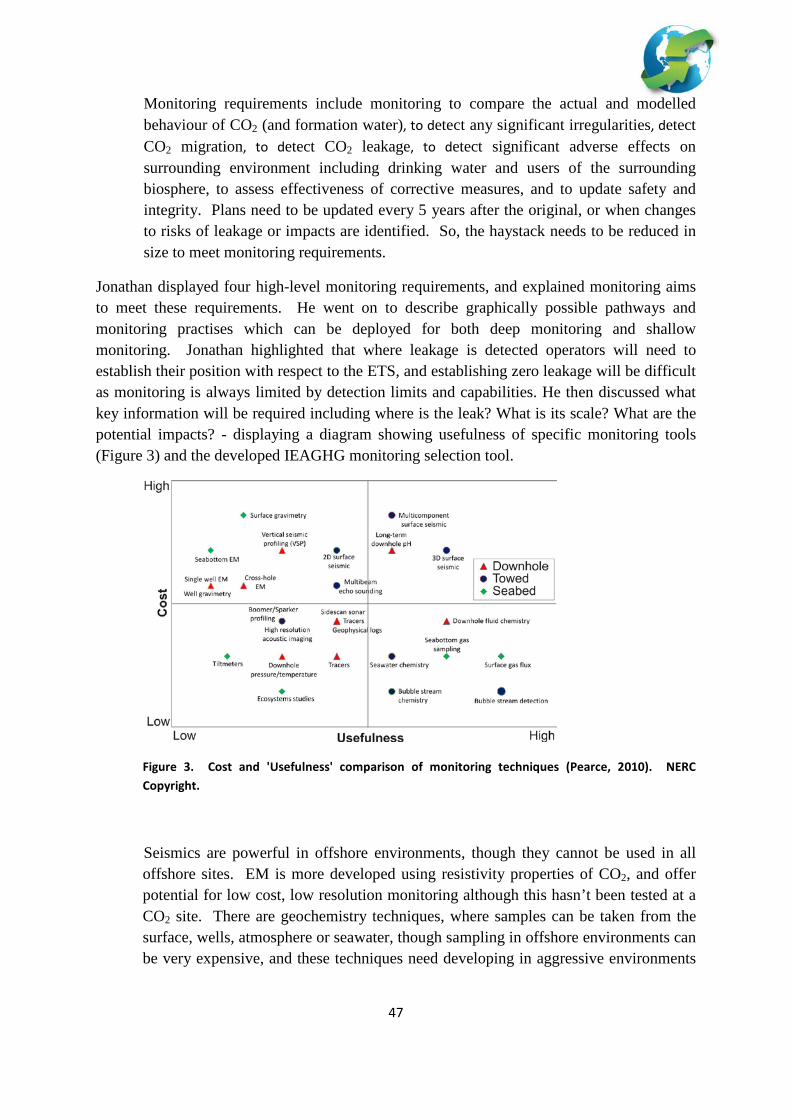
47

Monitoring requirements include monitoring to compare the actual and modelled behaviour of CO2 (and formation water), to detect any significant irregularities, detect CO2 migration, to detect CO2 leakage, to detect significant adverse effects on surrounding environment including drinking water and users of the surrounding biosphere, to assess effectiveness of corrective measures, and to update safety and integrity. Plans need to be updated every 5 years after the original, or when changes to risks of leakage or impacts are identified. So, the haystack needs to be reduced in size to meet monitoring requirements.

Jonathan displayed four high-level monitoring requirements, and explained monitoring aims to meet these requirements. He went on to describe graphically possible pathways and monitoring practises which can be deployed for both deep monitoring and shallow monitoring. Jonathan highlighted that where leakage is detected operators will need to establish their position with respect to the ETS, and establishing zero leakage will be difficult as monitoring is always limited by detection limits and capabilities. He then discussed what key information will be required including where is the leak? What is its scale? What are the potential impacts? - displaying a diagram showing usefulness of specific monitoring tools (Figure 3) and the developed IEAGHG monitoring selection tool.

Figure 3. Cost and 'Usefulness' comparison of monitoring techniques (Pearce, 2010). NERC Copyright.

Seismics are powerful in offshore environments, though they cannot be used in all offshore sites. EM is more developed using resistivity properties of CO2, and offer potential for low cost, low resolution monitoring although this hasn’t been tested at a CO2 site. There are geochemistry techniques, where samples can be taken from the surface, wells, atmosphere or seawater, though sampling in offshore environments can be very expensive, and these techniques need developing in aggressive environments

48

and for identification of limitations. None of these techniques will be used in isolation, and there isn’t a best technique or a single approach.

Low leakage rates may be very challenging to detect, and flux rates will vary over time so will need some sort of continuous monitoring. It will need areal coverage and linear coverage, and it will be important to be able to identify the source of the CO2. For the ETS, quantification will require a combination of techniques, accurate measurement of leakage rates, including temporal variation and integrated with areal coverage, and estimation of errors to allow calculation of allowances to be surrendered.

Jonathan concluded by highlighting that deep-focussed technologies are generally mature and demonstrated, other techniques (e.g. gravity) are less useful offshore because of high costs, shallow-focussed technologies are well developed onshore but need developing offshore, and detection and quantification of leakage at the seabed is a priority area.

5.1.3 Overview of Monitoring Controlled Releases

Lee Spangler, Montana State University

Controlled releases have many advantages for research including that they will typically have limited depth or overburden (and the overburden can be characterised in detail), flow rates can be known and controlled and so you can determine the onset concentration. You can determine the recovery time for responses, investigate changes in ecology due to high CO2, plus you can establish detection limits for monitoring technologies, and use them as a test bed for new technologies.

This new ZERT site is on agricultural land owned by the Montana State University, about 30 acres in size. The goal of the project is to develop injection rates for testing near-surface monitoring techniques. When you design a site you want to design your system to inject relevant injection rates. We put in a 100 m pipe and worked on 0.001% leakage, approximately 1 tonne per day, dividing into 6 zones using a packer system. These 6 zones can be controlled individually using mass flow controllers. We have had above ground lidar systems and plant flux investigations, and last year in the summer we had as many as 47 investigators from around 15 different institutions, using 31 instruments or sensor arrays.

Lee displayed a grid outlay of the experimental controlled release site, highlighting flux chamber measures in Jennifer Lewicki’s work, and presented some techniques which are under development including an underground fibre sensor with hollow core sections where the light interacts with CO2, and hyperspectral imaging which has the potential to be flown for large area surveys; displaying research undertaken last summer which although was very wet and therefore hyperspectral imaging wasn’t as effective as it could be though some plant stress hotspots could still be seen.

49

As for other controlled release sites, there is the University of Nottingham ASGARD site, which is much more set up for physiological responses, and it is better to look at specific plant responses at these small area sites. They have plot of 2.5 x 2.5 m, and 4 gassed plots per experiment with 4 ungassed controls, and they use various monitoring techniques including plant root photography and canopy measurements of CO2 using Draeger tubes.

CO2FieldLab involves shallow injection (10-30m) and deeper injection (200-300m), at a site in Norway, injecting 200 tonnes in two weeks. Here the drilling has been completed, and there will be an injectivity test in December. The project will be looking at various technologies such as ERT, seismics, NMR, EM, monitoring isotopes, pressure, temperature, and soil/surface monitoring such as using accumulation chambers and analysing bacteria activity.

There is a planned project in the USA at the Plant Daniel Test site, in Australia there is the Ginninderra Controlled Release Facility, a CO2CRC-Geoscience Australia project with a maximum release of 600 kg per day, and in Brazil the project is now back on, with a proposed site at the Ressacada’s Farm of Federal University of Santa Catarina (UFSC) which is a brown field site, proposing similar injection rates to those at ZERT.

It will be interesting to see the upcoming results from these projects, and importantly, natural and controlled release communities should work together to advance knowledge in this field.

5.1.4 CO2 leakage quantification methods: advantages and limitations

Sevket Durucan, Imperial College London

Sevket introduced the presentation by highlighting that this is an IEAGHG study which is currently underway by CO2GeoNet and led by Anna Korre at Imperial College London. He presented the main objectives of the study which were to identify and review the potential methods for quantifying CO2 leakages from a geological storage site from the ground or seabed surface, and discuss the level of accuracy that is currently required for site permitting and accounting purposes. He explained the specific tasks of the study, and detailed the specific monitoring methods presented in the study highlighting their usefulness in a summary table, and highlighted which partners were responsible for the particular tools discussed in the study. Sevket went on to explain in more detail the strengths and weaknesses of each monitoring tool, for example 3D/4D seismic which have a high degree of overall coverage, as well as high azimuthal coverage and a large offset interval, however noise is typically caused by non-repeatability in the acquisition and image-processing of the time-lapse 4D seismic surveys is difficult and demanding.

50

Regulatory requirements were then described for CO2 leakage quantification, including the EU ETS calculations, the US EPA Monitoring, Reporting and Verification (MRV) plan, and the Australian Ministerial Council on Mineral and Petroleum Resources (MCMPR) 2005 Regulatory Guiding Principles for CO2 Capture and Geological Storage; and he discussed that preference should be given to methods that are concurrently employed for performance monitoring, are favourable in terms of cost and benefit, are reliable and accurate, that can be deployed in conjunction with other monitoring techniques, can be operated autonomously or involve minimum human effort, are robust and low-maintenance, and have added benefit in improving the calibration of models.

Sevket concluded it is difficult to quote a generalised numerical value for accuracy in quantification across the board for all storage environments and monitoring methods and, most methods are unable to detect/quantify leakage at “low” rates (100 g/d); some methods may detect at “intermediate” rates (100 kg/d) on a case by case basis; and most methods considered can detect leakage at “high” rates (100 t/d), therefore, and on cost/benefit considerations, a portfolio approach is recommended. Specifically referring to monitoring tools he also presented conclusions from the study which highlight 4D seismic methods combined with Tiltmeters/InSAR and Downhole P/T monitoring may provide better leakage quantification with reduced uncertainty for reservoir and overburden monitoring; hydrochemical monitoring combined with flux measurements and the use of tracers/isotopic analysis may be the most appropriate for the shallow subsurface; plume profiles obtained with sonar methods combined with chemical analysis and the use of current meters may reduce uncertainty in the marine environment, as may soil gas analysis combined with flux measurements, the use of tracers/isotopic analysis and meteorological monitoring for surface or atmospheric monitoring.

5.2 Part II Chaired by Lee Spangler, Montana State University

5.2.1 Soil-gas behaviour and measurement in a carbon-reactive natural analogue; implications for near-surface monitoring

Katherine Romanak, The University of Texas Gulf Coast Carbon Center

Katherine opened by acknowledging the US DOE, the Gulf Carbon Center, The University of Texas at Austin and Dr. Philip Bennett from The University of Texas at Austin. She then explained using a diagram the different monitoring needed at a carbon dioxide storage site, including reservoir monitoring where most of the variability comes from the injection of CO2, and groundwater/vadose zone monitoring which has greater variability as the environment is dynamic and hence is difficult to monitor.

51

For monitoring in the vadose zone the main goals are to ensure the ability to detect early signs of leakage hence small shifts in CO2 concentration, to identify or characterise pathways of preferential transport, to develop cost-effective monitoring strategies and to provide information useful for remediation and accounting.

The near-surface is extremely dynamic relative to factors such as rainfall, barometric pressure changes, and biological activity; therefore there are some significant challenges. CO2 is highly reactive and mobile in the subsurface, and how do we determine what is being measured given natural variability and reactivity? We need to understand factors which create variability and this variability will determine the sensitivity of the environment to exogenous CO2 input.

To further understand this we used simple fixed gases to understand the environmental factors affecting CO2 concentrations at a playa lake.

Katherine described carbon cycling in the Vadose zone, where some processes produce or concentrate CO2 which can mimic a leakage signal giving a false positive, and others can consume or disperse CO2 dampening the signal giving false negatives.

Playa lakes are shallow circular basins that collect runoff from the surrounding flat plains and transmit that runoff into the soil. They are perched features and do not intersect with groundwater, so there is a thick vadose zone beneath these lakes for studying soil gas. In the soils beneath the lake, up to 17 vol % CO2 is formed by the oxidation of organic matter, transported through small cracks and root tubules, and this creates a “leakage signal” for the study.

The playa is ephemeral and exhibits considerable temporal and spatial variability in water flux and spatial variability in other environmental factors that can greatly affect soil gas CO2, such as organic carbon and soil carbonate. Starting from outside the playa slope and moving across the annulus and onto the playa floor, moisture, soil carbonate and organic carbon generally increase.

We sampled soil gas using multi-depth semi-permanent soil gas wells set in transects across the playa zones to understand how variability of environmental factors affects soil gas. Comparison of CO2, O2, and CH4 indicates that CO2 is primarily produced by oxidation of organic matter and this oxidation can be so vigorous at times as to produce CH4, especially when wetting fronts block vertical gas permeability and prohibit atmospheric oxygen from invading the soils. In some areas, this CH4 may be re-oxidized to CO2. Relationships among CO2, O2 and N2 show a significant CO2 sink in the playa floor: co-variations between CO2 and N2 in each zone show near- atmospheric concentrations of nitrogen in the slope where CO2 production and water flux is the lowest. In the annulus, N2 concentrations are mostly near atmospheric concentrations except for samples collected during high water levels, when water infiltrated through the annulus and we see a real enrichment in nitrogen

52

concentrations in the floor. We investigated denitrification as a possible cause but found this to be insignificant in playas.

This tells us CO2 is dissolving in the water, and reacting with the soil carbonate. The loss of gaseous CO2 into water creates a drop in the total pressure within the pore causing advection of air into the pore space and an overall increase in volume percent nitrogen above atmospheric concentrations. Other researchers have looked at nitrogen. For example at Weyburn, gas concentration relationships showed only microbial production of CO2 with N2 at atmospheric concentrations. In the playa, we have been able to identify both microbial oxidation of organic matter which does not affect N2 concentrations, and dissolution of CO2 which creates high N2 concentrations.

In the absence of soil carbonate, the dissolution of CO2 is simply a partitioning effect that is governed by Henrys law. At any given temperature, CO2 will partition itself between the gas phase and the water phase, but in the presence of soil carbonate, the dissolution of CO2 becomes a chemical reaction where CO2 reacts with soil carbonate and water to form dissolved ions. As long as there is CO2 and soil carbonate the reaction can continue and significant amounts of CO2 can be dissolved.

Katherine concluded by stating: water flux, organic matter and soil carbonate can be major factors influencing background CO2 concentrations in a system. Measuring all fixed soil-gases such as O2, CH4 and N2 in addition to CO2 and can give information on important Vadose zone processes affecting CO2 background concentrations. One-time measurements of parameters such as soil organic matter, soil carbonate, and moisture flux may be a simple way of characterizing a site for its "Surface Monitoring Potential", and "Surface Monitoring Potential” may give an indication of the sensitivity of the system to exogenous CO2 input.

5.2.2 Otway Project Monitoring

Charles Jenkins, CO2CRC and CSIRO

Charles introduced Otway as the very first of its kind, with a very comprehensive monitoring program, highlighting it has stored 65000 tonnes in the 3 years it has been running in Victoria, Australia.

There are several elements in the monitoring program which includes seismics, microseismics, fluid sampling, ground water and soil gas monitoring and, atmospheric and pressure monitoring. From the seismic results, there was nothing detectable above noise at the reservoir level, as it is a depleted gas reservoir there is little acoustic difference when replacing gas with CO2; and results are consistent with all forward models. We performed some hypothetical monitoring to see whether a set leakage rate would be detectable, and this suggests a point leak of approximately 5000 tonnes should be detectable. The most likely can be identified in the brightest colour

53

in the seismic plots. Tracer data worked well in the beginning but not towards the end of the injection and time lag is a large uncertainty.

The storage site is in a farming area with a lot of limestone. People are concerned about their water, and hence groundwater monitoring provides part of an assurance programme. We have no predictions for the groundwater, as we expect no leakage into the groundwater, but there is a lot of variability in the groundwater which is both natural and man-made through agriculture. We sampled all wells twice a year, and showed no changes above spatial and temporal variability in key indicators (pH, EC, HCO+). Tracers used are below the detectability limit. The bicarbonate shows some statistical difference, but not a lot.

We had a program measuring soil gas, with a matrix of locations now repeated yearly, and showing good results since 2008. There are a wide range of concentrations of CO2 but there is a repeatable correlation with δ13CO2. As for atmospheric monitoring, we have measured the atmospheric CO2 concentration downwind from the injection site for around three and a half years of near-continuous monitoring. There have been two ‘releases’ detected, one from the drilling rig and one from venting, with a sensitivity of around 1000 tonnes per year. We also had a microseismic array which failed, and a downhole pressure sensor which also failed leaving only downhole injection pressure available.

These results are used to answer questions including is there a leak? but you selected the site because there was limited possibility of a leak, so the probability is low and it is very difficult to detect such low permeability events. The questions we are trying to answer needs to be more tightly defined, such as: do we see excess CO2 in soil gas near the well? or, are there pressure anomalies? For: is there a leak that affects me here, now? soil gas and shallow groundwater monitoring can answer this but their sensitivity isn’t clearly defined. We don’t want to look for small anomalies and so we should say there has been no change within statistical variability. Some process must be understood to go from the measured amount to the X amount of CO2. We need to calibrate the techniques with the process. However, we may find ourselves going into an enormous research project due to all the various interactions within a system.

Charles concluded by highlighting some key learnings from the Otway monitoring programme: a M&V programme should be focussed on quite specific risks; it is important to have a plan as much as a program, i.e. if something was detected what would you do, and the thresholds of significance needs to be defined in advance; and measurements should be for well-specified purposes, with a plan for interpretation laid out in advance.

54

5.2.3 Regional and site-scale baseline surveys of near-surface gas geochemistry parameters - understanding natural variability as a framework for monitoring programs and public acceptance

Salvatore Lombardi, ‘La Sapienza’ University of Rome

Salvatore introduced his presentation by stating the best way to ensure public safety is by direct concentration and flux measurements although biological production of CO2 may influence these measurements and we need to understand this baseline.

In the early 1990s we had 10 stations at Latera at 0.5 m to 2.5 m depth. It was difficult to interpret the results. We repeated at a depth of 25 m, injected CO2, and again found the behaviour of CO2 was different. Perhaps a statistical approach can reduce the uncertainties.

We need to understand the baseline for site security. This is important for public acceptability and carbon credit auditing. In Italy people are living with CO2, for example in the region Ciampino, a town of 100,000 inhabitants in the volcanic area of the Alban Hills, and here there are two populations: those that understand the risks and those who know nothing about gas seepage in the area: two completely different groups.

Natural baseline variability will be from shallow natural sources which are typically from plant root and microbial respiration influenced by climate, topography etc, and deeper natural sources can result from groundwater degassing, CH4 oxidation, and natural CO2 accumulations regulated by lithology, structural geology and hydrogeology. The influence of these parameters will depend on scale and location, for example, cooler wetter climate in northern Europe versus warmer dryer one in southern Europe.

We need a framework with a database which describes the spatial and temporal conditions, protocols to ensure a statistically and spatially representative sampling of the study area, and chemical parameters for migration and impact models. For this we can conduct regional surveys based on different samples from different settings and repeat for different climatic effects, detailed baseline studies and detailed work on high risk areas. One example of this is Weyburn, where several surveys were undertaken, and two detailed profiles were established. Here, a suite of data was collected for a range of soil gases including nitrogen, helium, CO2 etc. You can see the values decrease with the sampling campaign (later in the season), and shows how a site can have a wide range of natural CO2 concentrations. When we use the same weather conditions the data is reproducible. There is significant variation in the summer season (when there is higher humidity), and values decrease from July to October.

More examples are shown in the URS Italian database which is a statistical approach to the study of gas migration in Italy. The map shows grey areas where oil and gas

55

have been discovered. Soil gas samples have been collected throughout central-southern Italy during the last 25 years for various projects, and the database consists of more than 35000 samples for helium and more than 15000 for CO2 and CH4.

Salvatore went on to show a series of normal probability plots for CO2 data from the URS database, divided on the basis of the type of geological setting, including volcanic areas, foredeep basins, Intramontane basins, and Neogenic basins. He explained the red line shows volcanic areas which vary up to 100%, and the green line is CO2 found on the Adriatic margin from oil or gas fields.

We see the behaviour is similar when you look at the normal variability decreasing from 20-0.25%, so this is the normal background for Italy. In the Vasto area; an exploited gas reservoir system in western Italy; a survey from 1987 to 1988 showed large anomalies corresponding with regional faults with 10-50% variability. A second survey was conduced in 2004 to 2005 in the same area but after depressurisation, which showed an overall decrease in concentrations and shows how baseline surveys can change with human intervention.

Salvatore concluded by emphasising the importance of baseline near-surface gas geochemistry data, which is crucial to interpret near surface monitoring results, carbon credit auditing, site security, public outreach, and owner liability.

5.2.4 Discussion Session 6

Panel Members: Ingo Moeller, BGR; Jonathan Pearce, BGS; Lee Spangler, Montana State University; Sevket Durucan, Imperial College London; Katherine Romanak, The University of Texas Gulf Coast Carbon Center; Charles Jenkins, CO2CRC and CSIRO; Salvatore Lombardi, ‘La Sapienza’ University of Rome

Q (for Katherine). Did you measure groundwater flow, and what is the reason for the drawdown?

A. It has 60 meters of unsaturated zone and the groundwater table is very deep. The lakes are ephemeral, they perch water that runs off of the High Plains. I did not use piezometers but others have.

Q (to Katherine). Are you aware of the Hannover-Hasselback equation, and did you measure the pH as this may explain why you don’t see CO2?

A. Yes I did take pH measurements in the lake, but all the interactions between CO2 and soil carbonate happens at depth. The soil carbonate is shallow outside the playa where infiltration of CO2 is low; however, soil carbonate is mobilized downward beneath the playa floor as it dissolves in areas of high CO2 and re-precipitates in areas of low CO2. We see this process of CO2 dissolution reflected in N2 concentrations, but the water in the lake does not come into

56

contact with the high CO2 concentrations and so lake water has a pH of about 7.5 and decreases for pore water within the sediments.

C. At every site you have groundwater and surface water, and then at a critical point when saturated you will have transfer to the soil. Degassing will only affect atmospheric gases. I would concentrate studies in the aquifer, as there you will see the first anomalies.

Q (to Jonathan). You discussed monitoring concepts and spoke about monitoring in marine and terrestrial environments: what about in sites close to shorelines? – could you combine both offshore and onshore methods? How can we register the transition between onshore and offshore techniques?

A. Yes, this it is a challenge to integrate the different techniques.

Q (to Jonathan). Do you think a 7.5% uncertainty is achievable?

A. This is extremely challenging. This number was arrived at politically not technically.

C (to Jonathan). If I should monitor 100km, this would need a huge amount of resources.

A. Yes, it is impossible to cover such wide areas with the more specific monitoring techniques, and it would be important to use the more sophisticated techniques to pinpoint the area to perform more detailed monitoring.

Q. The ETS suggests the operator defines the method of defining the uncertainty but with a plus of 7.5%, so, if you can do better than 7.5% is this extra cash in your pocket?

A. Yes.

Q (to Ingo). Is it a yes or no answer that you get about the size of the bubble and gas composition of the bubble with hydroacoustics or echosounders?

A. You can’t detect the composition of the bubble. You can see the difference in the size of the bubble.

Q. You showed some plots about the likelihood of the bubble making it to the surface – were these model results, and if so how accurate are these?

A. These were model results based on actual data. The theory is well understood and bubbles behave as expected.

C. Another system you can use is once you have detected the bubbles you can use a hydrophone which can detect the noise and composition.

C. In reference to the quantification study, if anyone is interested in reviewing the draft report, please contact us, and I have a question for the leakage rates – what made you choose the metrics?

57

A. They were based on natural flux rates on analogues on small sites and large sites, building on experience within CO2GeoNet. There are a lot of references to site specific results.

C. You may expect a different set of numbers based on climate change impacts.

C. The bottom line is site specific, and this is costly if you have to characterise all sites before actually doing CCS. We are craving a global tool, but it isn’t appearing.

C. The methods are expensive because we are using research budgets, but in a storage projects the costs will be much less in regards to the total cost, so we should bear in mind the legal requirements and industry scale. Perhaps the regulators will require expensive tools. The costs are not a limiting factor.

C. Even in the States, if you look at the chain, monitoring costs are minor and we can do excessive monitoring.

C. It will depend on the cost of carbon.

Q (to Lee). I’d just like to remark on monitoring for assurance. I have a lot of operators who don’t want surface monitoring because they are worried about the public response.

A. It was to test the detection technologies to see if they are effective, not to monitor a storage site. Regulators want to know if these methods are effective. We do, of course, have the issue of background variability. These were deployed at pilot sites, and we needed to test these on other sites.

Q. Are you able to do background monitoring at the same time as injection?

A. Probably not, as leaky wells need to be identified. When starting to build infrastructure it would be possible to start monitoring at that point.

C. There is no obligation at all to do baseline monitoring, though it is in your own interest.

Session 6: Outcomes and Recommendations Chaired by Ameena Camps, IEAGHG and Franz May, CO2GeoNet/BGR

Each of the session chairs prepared a brief presentation to summarise the main messages from their session, and these were presented, discussed and agreed upon by the workshop participants. The following encapsulates the key messages from each of these presentation summaries.

Session 1: Setting the Scene

Existing regulations, i.e. the OSPAR and London Protocol/Convention needed to be amended to ensure they did not prevent CCS configurations. There are now regulations in place

58

specifying the need to monitor and detect leakage and impacts, both in the EU CCS Directive to detect and measure impact, and in the ETS Directive to quantify leakage. A crucial word – ‘significant’ is used in both OSPAR and the EU CCS Directive which are difficult to define and leaves us with uncertainty – the research community are asked to provide information to move this forward. In the U.S. there are no clear regulations in place, and this is different in different States; though there are draft requirements in place e.g. the US EPA draft rule. Canada is ahead of the U.S. in regulating CCS, and the main blockers to U.S. legislation seem to be the question of pore space ownership, liability and transboundary movement with pipelines. The EU RISCS project will provide information to underpin evaluation of the safety of a storage site, to define critical risks, for environmental impact assessments; for safe design of a site to minimise impacts, design of near surface monitoring strategies, refining of storage license applications and frameworks for communication; focussing on natural analogues and experimental injection sites.

There have been various studies on natural release sites from volcanic regions and CO2 accumulations in sedimentary rocks, which can be used to learn where CO2 leakage is more likely to occur; the structural or geological controls on leakage should any occur (i.e. releases seem to be related to faults which can be self-sealing); potential rates; spatial-temporal scale an transport processes; how humans, plants and animals are impacted; mitigation strategies and, the most cost effective design of monitoring techniques.

Session 2: Releases, magnitudes and impacts (Marine)

Much can be learnt from knowledge transfer between ocean storage, ocean acidification and marine seepage research. In terms of chemical processes, a decrease in pH is noted by approximately two pH units and there are sites of extreme low pH due to hydrothermal fluid venting; CO2 bubbles may dissolve in the water column before reaching the atmosphere though this would still be classified as leakage out of the ‘storage complex’ under the ETS and EU CCS Directive; and hydrate formation may be possible in deep cold environments. Research on biological impacts note decreases in biodiversity with enriched CO2 environments and changes in species particularly loss of calcareous organisms; however species may cope if there is sufficient energy provided from other sources.

Monitoring technologies are sufficient to detect CO2 bubble streams for example hydroacoustics and to monitor chemical effects (e.g. pH, pCO2), though technologies to assess impacts are still being developed or are currently being applied, for example ROVs. Natural analogues do have limitations, including that they may be ‘steady-state’, response rates and recovery rates are difficult to establish as they are ‘mature’ sites, and it is uncertain whether scales are realistic for storage; hence it is important to recognise the limitations as well as the benefits and maintain the context. Experimental programmes are needed to understand the key processes, especially on responses to changing conditions, and research to test measurement technologies at analogue sites.

59

Session 2: Releases, magnitudes and impacts (Terrestrial)

Moffettes, sites with pure CO2 emissions which are pre/post volcanic or metamorphic in origin, can be mapped quite accurately by the mapping of plant and soil-animal species. The adaptability to increased CO2 concentrations is different for different species: animal species may respond more quickly but plant stress can be identified remotely. It may even be possible to identify concentrations as well, by understanding the impact on specific animal and plant species. There are many ‘moffettophilic’ and ‘moffettophobic’ plants and it may be possible to identify these indicator species globally for other storage relevant regions. A portfolio of different methods is recommended for detection, quantification and system understanding at various scales, and more research is needed on the groundwater impact by subsurface fluids with or without CO2.

Session 3: Mobilisation of Brine and Metals

Various different analytical tools are needed to determine the effects of CO2 injection, and monitoring tools are needed to determine what is being mobilised for which existing sensors to be improved, new sensors need to be developed and new applications, such as for biological and geophysical modelling need to emerge. Integration of laboratory, field and modelling studies, both for analogues and pilot projects, is needed in future additional research for further understanding crucial to update current risk assessments regarding mobilisation of metals which may be inaccurate. Research focussing on an aquifer near Chimayó, New Mexico, USA, which contains natural sources of CO2, found the presence of trace metals was more closely associated with brackish water than in-situ mobilisation of trace metals; hence the intrusion of brackish water displaced by CO2 could be more important and needs to be researched further. Pure modelling research examining the effects of impurities injected in the CO2 stream found increased groundwater acidification and following increased dissolution of different substances resulting in Health Specific Impacts: therefore the concentration of impurities may influence dissolution processes of trace metals in the storage reservoir which will be particularly important for pipeline systems integrating multiple sources of CO2.

Session 4: Near Surface vs. Deep Subsurface Mechanisms

Care is needed when making direct links between analogues and CCS systems. A large amount of energy is required for large scale CO2 seal breech, and as such in geological systems not all leaks reach the surface. Outcrop studies can impart important information to the study of natural analogues. Escaping CO2 from the deep subsurface is commonly trapped in ‘reservoirs’ at 500-1000m depth. CO2 accumulations and releases have been associated with seismicity and therefore may provide important information in regards to the possibility of induced seismicity associated with injection and storage; and high CO2 fluxes through aquifers is possible, as has been seen at natural sites in Italy. Water chemistry bears the signal of reactions during the CO2-water migration from depth, and it is possible to measure the magnitude of CO2 charged fluids required to impact near surface water systems using natural analogues though this is highly site specific. It is also possible to study near surface

60

mitigation of CO2 leaks using natural analogue sites as ‘test’ sites, however there may be attachment to some natural release sites and hence public opinion to such would need to be explored further.

Great advances have been made in monitoring CO2 storage in the subsurface; an example of such would be monitoring the CO2 plume at Sleipner. Monitoring results can be used to calibrate transport models which are iterative and regulations stipulate recalibration of such with time. Most importantly we need to understand the system, and some of this information can be gained from natural analogues or controlled release sites. In terms of microbiology, there is a systematic response to high CO2 concentrations, and understanding this response is critical to the implementation of CCS.

Session 5: Monitoring challenges in light of natural systems

Finding a leak is difficult due to the scale of storage projects (‘finding a needle in a haystack’), though seepage is relatively easy to detect in a marine environment due to the differences between the physical properties of CO2 and seawater. Hydroacoustical methods have been successful at detecting natural CO2 seepage from the seabed. Development of a shallow monitoring strategy should be an iterative process based on the feedback from primary deep monitoring tools, and a monitoring portfolio that includes currently available methods that detect, quantify and reduce uncertainty is recommended. Controlled releases can provide additional information which compliment natural analogue studies, and there are more sites which are starting to be investigated.

The near surface (vadose zone) is dynamic and background variation is complex, hence highlighting the need to establish and understand good background data and its variability. Processes and their variability is site specific, hence there is a need for more site investigations to enable the establishment of a complete dataset. Other gases may provide valuable information, for example nitrogen and oxygen, and monitoring should address multiple requirements. Poorly understood datasets may represent a political or public perception challenge.

These summaries were brought together in an open discussion to identify the recurring learnings from all of the sessions. The recurring learnings were identified as:

• There is a need to integrate field, laboratory and modelling work.

• There are a range of variables, so we need to understand the system, i.e. what is common and what is different.

• There is a need to further understand the hydrogeochemistry/hydrogeology/hydrodynamics.

61

• There are species which can be clearly identified as indicator species and there is a need to draw these together into an indicator species database.

• There is a need to integrate current research in various natural analogue studies for a focussed research program.

Drawing from all the sessions, the key knowledge gaps were highlighted as:

• There is a need for further understanding of impacts and processes of CO2 displaced waters.

• There is a need to further understand the physical processes of CO2 flow in aquifers.

• There is a need to draw together studies to produce an indicator species database.

• Field studies are needed to investigate potential mobilisation of brine and metals.

• There is a need for more data on natural background CO2 in offshore environments.

• There is a scarcity of data on long-term impacts of CO2 due to time limited research.

• Further understanding of mechanisms in the deep subsurface from natural analogues is needed; particularly in regard to the understanding of caprocks and additional barriers and trapping mechanisms; drawing from research in other geological communities.

• There is a need to further understand the association of seismicity with natural accumulations of CO2.

Finally, the participants from the IEAGHG Workshop on Natural Releases of CO2: Building Knowledge for CO2 storage Environmental Impact Assessments recommend:

• Now there is an IEAGHG research community established, and especially given the tight scheduling of this meeting agenda due to considerable interest, a follow up IEAGHG meeting is recommended (perhaps additionally a dedicated session focussed on impacts at AGU).

• An integrated, international, cross-disciplinary natural analogue/controlled release program given the wide spread of researchers who can impart knowledge to advance knowledge in this critical research area.

• Future and current research needs to integrate modelling, field studies and laboratory research.

62

• Further research on long-term impacts in marine and terrestrial environments.

• It is important to expand this community to include other areas of relevant research bringing together biologists, geologists and many other experts to advance knowledge, as has clearly happened at this workshop.

Field Trip Overview

The third day of the Natural Releases workshop was spent in the field, starting with a 6 km walk around Laacher See (a volcanic centre of the East Eifel field). During this walking tour, various stops were made around the lake and caldera to observe geological outcrops, CO2 bubbles in the lake itself and mofettes identifiable by features such as swampy muddy areas, the presence of different organisms or differing appearances of certain plant species. Here, ecosystems have appeared to adapt to the differing CO2-related conditions through species substitution and adaptation.

Hardy Pfanz from the University of Duisberg-Essen pointed out the stunted growth and discoloration of some species or presence/absence of certain species where there was a flux of CO2. Other signs of CO2 releases seen along the walk included CO2-rich mineral springs with slightly fizzy fresh water that tasted of Iron. It is thought that the CO2 degassing in the Laacher See area is related to upper crust anomalies through intrusion into the lower crust. Attendees were also treated to a first-hand demonstration of an accumulation chamber along with the collection of samples from the sediments in the lake by colleagues from BGR.

The afternoon of the field trip day was spent visiting springs at Waasenach and the Wallenborn geyser in the West Eifel region. The geyser proved to be an impressive sight, erupting CO2-laden water 4 metres into the air approximately every 30 minutes. It was explained the sizeable height of the water plume of this geyser was down to artificial engineering in the well which penetrates a natural CO2 reservoir. The specially-engineered well funnels the water out more forcefully and higher than would naturally occur at this particular point.

The day ended with a dinner at a local brewery (in the nearby town of Mendig), which is situated on top of former basalt mines. The whole field trip was a highly informative and enjoyable day (largely thanks to our host, the knowledgeable Franz May from BGR), giving all attendees a chance to experience and see some of the natural releases of CO2 in the area.