Storage SystemsStorage SystemsCSE 598d, Spring 2007CSE 598d, Spring 2007

Lecture 5: Redundant Arrays of Lecture 5: Redundant Arrays of Inexpensive DisksInexpensive Disks

Feb 8, 2007Feb 8, 2007

What is a RAID?

Why RAID?

• Higher performance– Higher I/O rates for short operations by exploiting

parallelism in disk arms

– Higher bandwidth for larger operations by exploiting parallelism in transfers

• However, we need to address the linear decrease in MTTF by introducing redundancy

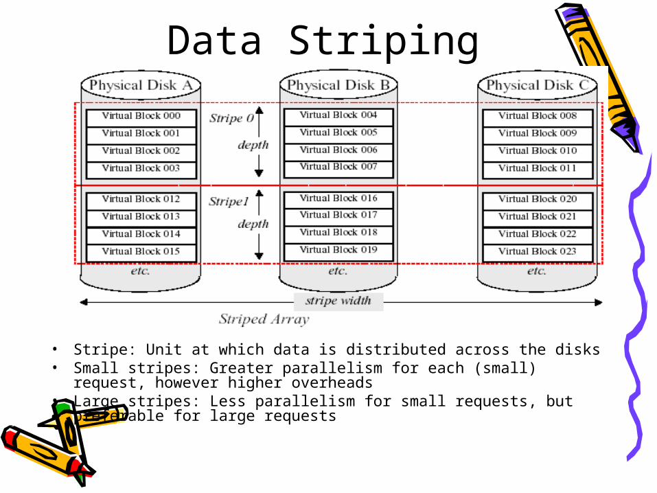
Data Striping

• Stripe: Unit at which data is distributed across the disks• Small stripes: Greater parallelism for each (small) request,

however higher overheads• Large stripes: Less parallelism for small requests, but

preferable for large requests

Redundancy• Mechanism: Parity, ECC, Reed-Solomon codes, Mirroring

• Distribution schemes:– Concentrate redundancy on a few disks– Distribute the parity similar to data

RAID Taxonomy/Levels• RAID 0 (Non-Redundant)• RAID 1 (Mirrored)• RAID 2 (ECC)• RAID 3 (Bit-interleaved Parity)• RAID 4 (Block-interleaved Parity)• RAID 5 (Block-interleaved distributed Parity)• RAID 6 (P+Q Redundancy)• RAID 0+1 (Mirrored arrays)

Non-Redundant (RAID 0)

• Simply stripe the data across the disks without worrying about redundancy

• Advantages:– Lowest cost– Best write performance, used in some

supercomputing environments

• Disadvantages:– Cannot tolerate any data loss

Mirrored (RAID 1)

• Each disk is mirrored• Whenever you write to a disk, also write to its

mirror• Read can go to any one of the mirrors (with

shorter queueing delay)– What if one (or both) copies of a block get corrupted?

• Uses twice the number of disks!• Often used in database applications where

availability and transaction rate are more important than storage efficiency (cost of storage system)

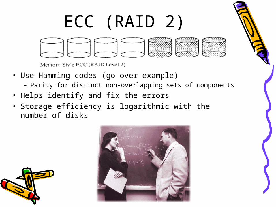
ECC (RAID 2)

• Use Hamming codes (go over example)– Parity for distinct non-overlapping sets of components

• Helps identify and fix the errors• Storage efficiency is logarithmic with the number of

disks

Bit-Interleaved Parity (RAID 3)

• Unlike memory, one can typically identify which disk has failed

• Simple parity can thus suffice to identify/fix single error occurrences

• Data is interleaved bit-wise over the disks, and a single parity disk is provisioned

• Each read request spans all data disks• Each write request spans all data disks and parity disk• Consequently, only 1 outstanding request at a time• Sometimes referred to as “synchronized disks”• Suitable for apps need high data rate but not high I/O rate

– E.g., some scientific apps with high spatial data locality

Block-Interleaved Parity (RAID 4)

• Data is interleaved in blocks of certain size (striping unit)• Small (< 1 stripe) requests

– Reads access only 1 disk– Writes need 4 disk accesses (write new data, read old data,

read old parity, write new parity) – read-modify-write procedure

• Large requests can enjoy good parallelism• Parity disk can become a bottleneck – load imbalance

Block Interleaved Distributed Parity (RAID 5)

• Distributes the parity across the data disks (no separate parity disk)

• Best small read, large read and large write performance of any redundant array

Distribution of data in RAID 5

• Ideally, you want to access each disk once before accessing any disk twice (when traversing blocks sequentially)

• Left symmetric parity placement

P+Q Redundancy (RAID 6)

• Parity requires single, self-identifying error• More disks => Higher probability of multiple simultaneous failures• Idea: Use Reed-Solomon Codes for redundancy• Given a set of “k” input symbols. RS adds “2t” redundant symbols to

give a total number of symbols “n=k+2t”– 2t is the number of self-identifying errors we want to protect against

• The resulting “n” sequence can:– Correct “t” errors– Correct “2t” erasures

• Error locations are known

• So if we want to tolerate 2 disk failures, we only need t=1, i.e. 2 redundant disks

• Performance similar as RAID-5, except small writes incur 6 accesses to update P and Q

Mirrored Arrays (RAID 0+1)

• Combination of “0” and “1”

• Partition the array into groups of “m” each, with each disk in a group reflecting/mirroring the contents of the corresponding disk in other groups. If “m=2”, becomes single mirror

Comparing the levels

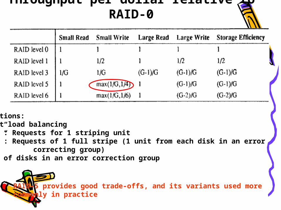
Throughput per dollar relative to RAID-0

Assumptions:Perfect load balancing“Small”: Requests for 1 striping unit“Large”: Requests of 1 full stripe (1 unit from each disk in an error correcting group)G: No. of disks in an error correction group

RAID-5 provides good trade-offs, and its variants used morecommonly in practice

Reliability

• Say the mean-time-between-failures of a single disk is MTBF

• Mean-time-between-failures of a 2-disk array without any redundancy is – MTBF/2 (MTBF/N for a N disk array)

• Say we have 2 disks, where 1 is the mirror of another. What is the MTBF of this system?– It can be calculated based on the probability of 1 disk

failing, and the second disk also failing during the time it takes to repair the first disk

– (MTBF/2) * (MTBF/MTTR)

• MTTF of a RAID-5 array is given by – (MTBF*MTBF)/N*(G-1)*MTTR

Reliability (contd.)• With 100 disks each with

MTBF=200K hours, a MTTR=1 hr, and a group size of 16, MTBF of this RAID-5 system is 3000 years!

• However, higher levels of reliability are still needed!!!

Why?• System crashes and Parity inconsistencies

– Not just disks fail. System may crash in the middle of updating parity leading to inconsistencies later on

• Uncorrectable Bit Errors– There may be an error when obtaining the data

from a single disk (usually incorrect writes) that may not be correctable

• Disk failures are usually correlated– Natural calamities, power surges/failures,

common support hardware– Also, disk reliability characteristics (e.g.

inverted bathtub) may themselves be correlated

Consequences of data loss

Implementation Issues• Avoiding stale data

– When a disk failure is detected, mark its sectors to be “invalid”, and after the new disk is re-created mark its sectors to be “valid”

• Regenerating parity after crash– Mark parity sectors “Inconsistent” before servicing

any write– When a system comes up, regenerate all

“Inconsistent” parity sectors– Periodically mark “Inconsistent” parities to be

“Consistent” – you can do better management based on need

• Orthogonal RAID– Reduces disk

failure correlations

– Reduces string conflicts

Next class: RAID modeling

• Improving small write performance in RAID-5– Buffering and Caching

• Buffer writes in a NVRAM to coalesce writes, avoid redundant writes, get better sequentiality, and allow better disk scheduling

– Floating parity• Cluster parity into cylinders each with some spares.

When parity needs to be updated, new parity block can be written on the rotationally-closest unallocated block following old parity

• Needs a level of indirection to get to latest parity

– Parity Logging• Keep a log of differences that need to be made to parity

(in NVRAM and on a log disk). Later on update the new parity

• Declustered Parity– We not only

want to balance load in the normal case, but also when there are failures

Say Disk 2 fails in the two configurations.The latter will more evenly balance the load

• Online Spare Disks– To allow reconstruction to start immediately (no

MTBR) so that window of vulnerability is low– Distributed Sparing

• Rather than keep separate disks (idling), spread the spare capacity around.

– Parity Sparing• Use the space capacity to store additional parity. One

can view this as P+Q redundancy• Or small writes can update just one of the parities

based on head position, queue length, etc.

• Data Striping– Trade-off between seek/positioning times, data

sequentiality and transfer parallelism– Optimal size of data striping is

Sqrt(P.X.(L-1).Z/N) where• P is the avg. positioning time• X is the avg. transfer rate• L is the concurrency• Z is the request size• N is no. of disks.

– Common rule of thumb where not much is known about the workload for RAID-5 is

½ * avg. positioning time * transfer rate