Store and Haul: Improving Mobile Ad-Hoc Network Connectivity through Repeated Controlled Flooding Robert Tyson Thedinger Submitted to the graduate degree program in Electrical Engineering & Computer Science and the Graduate Faculty of the University of Kansas School of Engineering in partial fulfillment of the requirements for the degree of Master of Science. Thesis Committee: Dr. James P.G. Sterbenz: Chairperson Dr. Joseph Evans Dr. Arvin Agah Date Defended c 2010 Robert Tyson Thedinger
Transcript
Store and Haul: Improving MobileAd-Hoc Network Connectivity through
Repeated Controlled Flooding
Robert Tyson Thedinger
Submitted to the graduate degree program in ElectricalEngineering & Computer Science and the Graduate Faculty of theUniversity of Kansas School of Engineering in partial fulfillment
of the requirements for the degree of Master of Science.
Communication is an integral part of any industry or society; as they inextri-
cably link more and more electronic devices into their systems, they increasingly
rely on communication networks. In every facet of life, from warfare to car pool-
ing, communication mechanisms are ubiquitous. While great progress has been
made in advancing the state of the art in communication networks, the challenges
of modern day networks have increased in number and complexity.
Mobile ad hoc networks (MANETs) are a type of mobile, wireless network
that does not rely on infrastructure. These networks contain freely-moving nodes
that result in dynamic and frequently changing topologies [1]. Their design incor-
porates all network functionalities within the MANET nodes, including routing,
forwarding, error control, connectivity, and security [2]. MANETs are often char-
acterized by their more pronounced challenges, the most notable of which are
dynamic topologies, bandwidth constraints, power constraints, and limited phys-
ical security [1]. While these challenges are somewhat daunting, the potential
benefits MANETs can offer communication networks make them attractive to
research and hold great promise for future networks.
2
These benefits of MANETs motivate novel ideas and innovative strategies. For
example, dynamic topologies have been met with new types of routing protocols;
proactive, reactive, adaptive, geographical, and power-aware routing protocols
have been developed to help combat some of the challenges described and are
outlined in Chapter 2. Most pertinent to this work is the Store-and-Haul (S&H)
paradigm [3], which uses the mobility of the nodes to carry transmitted data
across an episodically connected network.
1.1 Motivation
Traditional MANET research does not consider partitioned networks. Only
recently have potential solutions been proposed – most of which consider some
form of storing received data and hauling it to segregated areas of the network
for retransmission [4, 5, 6, 7]. However the majority of those S&H algorithm
and protocols have taken complex or memory intensive approaches; e.g. assigning
“ferry” nodes [5], connection-oriented approaches, or storing every message sent
in the MANET [4].
The goal of this thesis is to explore a new approach, that is easy to imple-
ment, systematically disseminates data throughout the network, requires minimal
memory, and yields notable packet delivery improvements over standard MANETs
protocols.
1.2 Thesis Methodology and Goals
The ultimate goal of this research is to determine the improvements possible
by implementing S&H in conjunction with other MANET routing protocols. The
3
goals of this thesis were limited to investigating S&H in conjunction with repeated
controlled flooding (explained further in Section 2.1), S&H+RCF (store-and-haul
with repeated controlled flooding):
1. Modify the ns-2 simulator so that network nodes will hold transmissions for
a specified time. The customized ns-2 software is also further modified to
repeat specified transmissions a specified number of times.
2. Construct reasonable scenarios of MANETs in which to run this new S&H+RCF
mechanism. Run the scenarios systematically and record the results for anal-
ysis.
3. Run baseline control simulations with conventional, controlled forwarding –
using the same MANET scenarios as used for the S&H+RCF simulations.
4. Analyze the results and compare control simulations with the S&H+RCF
simulations.
5. Characterize the S&H+RCF performance and draw conclusions.
1.3 Contributions
This thesis contributes the following:
• Offers and explores a new communication paradigm by combining store-and-
haul with repeated and controlled flooding
• Developed a new model in ns-2 to implement S&H+RCF
4
• Performs analysis on new communication paradigm to determine benefits
and tradeoffs for S&H+RCF and shows that S&H+RCF provides better
communication capabilities in disconnected networks
1.4 Thesis Organization
The rest of the thesis is organized as follows: the background of MANETs,
S&H, and RCF, as well as related work in the subject area are discussed in Chapter
2. Chapter 3 explains the S&H+RCF mechanism in detail. Chapter 4 describes
the simulations: network parameters, MANET characteristics, and S&H settings
for the different sets of simulations. Performance results of the simulations and
analysis of the benefits are outlined and discussed in Chapter 5. The thesis
conclusions and comments on future work to be done on S&H are discussed in
Chapter 6.
5
Chapter 2
Background and Related Work
MANETs vary greatly in their design, purpose, and operation. The factors
that affect and impact the success of MANETs are often as dynamic as the
MANETs themselves. Naturally, success greatly depends on the design objec-
tives and the challenges or constraints that might apply to a given scenario. To
better understand the basis of S&H+RCF, the different types of relevant MANET
methodologies and protocols are examined and studied. RCF (repeated controlled
flooding) was adapted from controlled flooding in MANETs – controlled flooding
has been common in communication networks for many years. S&H (store and
haul) has not been around as long and is a little more complicated. Some of the
first MANET protocols and methodologies that exploited the S&H concept had
slightly different objectives in mind than S&H+RCF, such as energy conservation
and lossless packet delivery, but most are similar enough that made their data apt
and applicable.
This chapter is organized as follows: the background and related work starts
by covering the oldest and more simplistic relevant research: controlled flooding.
It then delves deep into MANETs and the most popular MANET protocols. The
6
chapter then wraps up with a description of delay tolerant networking.
2.1 Controlled Flooding
Controlled flooding (CF) is one the simplest MANET routing algorithms in
network communications, much older than the concept of MANETs. CF begins
with the transmission of a packet by a source to all known neighbors. If the neigh-
bor is the packet’s destination then the packet is sent to the application. If the
neighbor is not the destination, the node repeats it to all known neighbors again
– except to the node from which the packet came [8]. CF is neither classified
as a reactive or proactive routing algorithm as it does not keep routing tables.
What matters most in the routing process is the identity of the source and des-
tination nodes [9]. The most important feature to note about CF is packets are
only transmitted to nodes that have not already received the packet [10]; this is
the difference between uncontrolled and controlled flooding. With this in mind, it
should also be noted that CF is a little more difficult in MANETs, because paths
are dynamic and frequently changing. Therefore, CF in MANETs may actually
begin to transmit the packet toward the node from whence it came. If the re-
ceiving node realizes it has already seen and transmitted the packet, the packet
is dropped immediately. Finally, it is not uncommon for CF to set limitations on
how many times a packet may be forwarded. Most often this is done with a Time
To Live (TTL) mechanism.
While it is more complex and advanced, Tiny Ad-Hoc Routing Protocol (TARP)
is based on CF [11]. TARP first inspects a packet to see if that particular node
is the packet’s destination. If it is, the packet is passed up to the transport layer
and the transmissions cease for that packet in that node. Otherwise, the packet is
7
then subjugated to three rules. The first, duplicate discard (DD), drops packets
when multiple copies have been previously seen and forwarded by the receiving
node. The second rule is suboptimal path discard (SPD), which drops packets
that have taken an “unreasonable” path between source and destination nodes.
The final rule is load balancing (LB), which explores alternative paths through
diversification. It accounts for possible congestion and works in tandem with SPD
by responding to mobility and calculating more “reasonable” routes. The three
rules are executed sequentially and are restrictive in nature. Their decisions are
based on packet characteristics that are embedded by the TARP protocol within
each packet header [11].
The header includes the source and destination addresses, the session identifier,
the sequence number of the session, the packet’s count, the maximum path length
the packet may travel in hops, and the number of hops the packet has traveled so
far. These characteristics are the packet signature that determines which packets
are acceptable to retransmit and which are not [11].
While the results of TARP ns-2 simulations varied depending on how the rules
were configured, it was outperformed by DSDV, AODV, and DSR. However, the
authors contend that it is still comparable to “serious routing protocols” with
relatively complex route discovery and maintenance techniques (DSDV, AODV,
DSR, etc.) [9]. TARP is designed as a maintenance free protocol for MANETs
that efficiently uses network resources. It may be best suited for MANETs that
employ small and inexpensive hardware [9] [11].
8
2.2 Mobile Ad Hoc Networks
MANETs are defined as a network with mobile nodes that can communicate
without any existing infrastructure. In other words, there is no need for towers,
satellites, or any kind of stationary, wired support system [1]. Arguably, there has
always been a need for MANETs but the real research for this type of network did
not begin until the late 1990s. MANETs are the progeny of research programs such
as Survivable, Adaptive Networks (SURAN) [1] and Survivable Communication
Networks (SCN) [1]. MANETs have been developed largely through the efforts
of DARPA and ONR (Office of Naval Research), which recognized the need for
communication networks in areas where existing infrastructure was not available,
too expensive, or impossible to deploy.
Not only have military and explorative organizations have noticed the possi-
ble benefits, MANETs have attracted the attention of commercial organizations
as well, particularly the need to communicate through harsh and remote envi-
ronments. From the rugged and threatening battlefields of future wars, to space
exploration, to remote scientific locations such as underground exploration or po-
lar research – MANETs provide the prospect of providing network connectivity
where the luxury of infrastructure is not practical [12].
These hopes and expectations placed on MANETs are often overshadowed by
the aforementioned challenges inherent to their design and function. Mobility is
the physical movement of a node or nodes which dynamically changes its points
of attachment to the rest of the nodes [13]. This results in the dynamic topologies
in which nodes move in and out communication range as shown in Figure 2.1.
Dynamic topologies are extremely problematic in network engineering because of
the difficulty involved in delivering the right information or packet of information
9
to the correct node. If nodes are moving they are often difficult to find and
sometimes out of reach for a period of time.
t2t1
57
1
9
8
4
2
6
3
5
7
1
9
8
4
2
6
3
Figure 2.1. Nodes moving inside of a MANET
The next two challenges are bandwidth and power constraints. They are
tightly interconnected as they often limit or exist because of each other. The
bandwidth constraints are due to a number of reasons. The wireless medium is
unreliable with greater limitations on bandwidth when compared to wired links.
While advances have been made in wireless technology to produce higher band-
width, the nodes are self-contained and have limited energy. Furthermore, the
nodes share the same medium, which results in sharing of the limited capacity
and the need for a MAC (medium access control) for arbitration [14]. As previ-
ously mentioned, the power constraints are mostly due to their self containment
and need for mobility. Typically powered by batteries, nodes in a MANET have a
limited amount of energy [15]. Another challenge is security; the wireless medium
has proven difficult to secure since its inception. Attempts to encrypt and secure
10
the wireless channels are often unsuccessful, as seen in WEP and now seen in
WPA [16]. The added complexity of dynamic topology makes security even more
difficult. The additional overhead incurred with trying to secure MANETs weighs
heavy on the extremely limited resources of power and bandwidth.
Network engineers meet all of these challenges in a variety of ways. The routing
protocol is integral to the success of a MANET. Just as there are many differ-
ent kinds of MANET configurations, constraints, obstacles, and limitations there
are many different kinds of MANET routing protocols that provide a potential
solution to each scenario.
The most common and well known MANET routing protocols are classified as
proactive or reactive. Proactive routing protocols keep a table of all possible paths
in the MANET at all times. This is sometimes referred to as “table driven” routing
and is accomplished with control messaging that monitors the paths. Reactive or
“on demand” routing is where nodes only learn paths when there is data to send.
Like many aspects of engineering, no one protocol is necessarily better than
another. Instead they are regarded as more suitable than another for a particular
scenario. The next four sections give brief backgrounds on some of the most
popular MANET protocols.
2.2.1 DSDV
DSDV (Destination-Sequenced Distance-Vector Routing) was developed for
mobile networks in 1994 by Perkins and Bhagwat [17]. Based on the Distributed
Bellman-Ford algorithm, DSDV has each node maintain a table that tracks all
the possible paths within a mobile network making it a proactive routing protocol
[17]. These tables are created from routing information that is shared between
11
nodes through updates. The updates are at first dumped to a node entering the
range of a mobile network with incremental updates to follow. The route selection
is performed using age and metric of the entries in the table.
As one of the earliest MANET protocols, DSDV has some significant draw-
backs – namely performance and energy consumption. However it did provide
guarantees of a loop-free path to each possible destination in the MANET and is
the basis for many modern MANET protocols.
2.2.2 AODV
As a successor to DSDV, AODV (Ad hoc On-Demand Vector routing) im-
proved on a number of aspects. Using reactive routing instead of proactive routing,
AODV reduced signaling overhead, collisions, and energy consumption. Perfor-
mance was also increased by the way AODV finds a desired route [18].
AODV finds a route by first broadcasting a request for the destination node.
This request is forwarded through the network keeping track of the path the
request takes. If the request reaches the destination node, a reply traverses the
same path back to the originating node. Assuming paths exist, the originating
node will receive one or more ways to the destination node. The originating node
will usually choose the path with the fewest hops and send the transmissions down
said path. If a link fails and the path is lost the process is repeated. [18]
2.2.3 DSR
Designed specifically for MANETs in 1994, DSR (Dynamic Source Routing) is
a reactive form of routing that attempts to improve route development and selec-
tion within a MANET’s nodes. DSR is essentially comprised of Route Discovery
12
and Route Maintenance. [19]
Route Discovery is performed by a sending node to find all the available paths
to a destination. It floods a route request throughout the MANET. If no desti-
nation is found the route request is re-flooded until a timeout is reached. If the
timeout is reached the data is either either queued for later route discovery at-
tempts or dropped. Route Maintenance is performed when a path is lost between
a source and destination. Essentially, Route Maintenance selects an alternate
path or reinvokes Route Discovery.
2.2.4 OLSR
As one of the modern proactive MANET routing protocols, OLSR (Optimized
Link State Routing Protocol) [20] is a canonical example of proactive and link-
state routing in MANETs. This protocol is table driven and begins by controlling
the topology. Topology control is established through a system of hello messages
multi-point relays (MPRs). MPRs are responsible for forwarding traffic and act
as a mechanism of control transmissions reduction. Each node selects a set of
neighboring nodes as MPRs and the MPRs declare all the link state information
to the rest of the network. These declarations provide shortest path routes to all
network nodes (and potential routes for redundancy).
2.3 Disruption Tolerant Networks
Delay tolerant networks (DTNs) attempt to facilitate communications when
connectivity is sporadic or discrete. This means that DTNs take a store-and-
forward approach [21, 22] based on the interplanetary network (IPN) framework
[23]. While the storing of data in DTNs has significant performance implica-
13
tions, its primary objective is to bring communication to systems in which there
previously was none. [24]
Disruption tolerant networks (DTNs1), is a generalization of delay tolerant
networking, encompassing network interruptions other than just delays. MANETs
share the property of episodic connectivity with DTNs. Furthermore, S&H in
MANETs is often sparsely connected or highly dynamic and can benefit from S&H.
The following sections describe different different S&H methodologies employed
by MANETs, presented in chronological order from when they were first described
in research.
2.3.1 Epidemic Routing
One of the first researched implementations of S&H is epidemic routing. The
protocol eventually achieves the optimal packet delivery ratio (PDR), given enough
time, described by the following formula:
limt→∞
PDR = 100%
Assuming that partitions do not persist indefinitely, all packets will be delivered
to their destinations in MANETs [4].
2.3.1.1 Epidemic Design
The main goal of epidemic routing is to transmit every packet to every node
once, and only once. Eventually, every transmitted packet should reside on every
node within the MANET. Epidemic achieves this by having the node keep an array
1The acronym DTN is used for both delay tolerant networking and disruption tolerant net-working
14
of all packets it generates and all the packet it receives. Each packet transmitted
throughout the network must have a unique packet identifier and the array is
indexed by that packet identifier. In addition to the packet identifier, the epidemic
design calls for a hop count, and an optional acknowledgment request [4].
Epidemic is designed to only transmit each packet once to every node in the
network, achieved through a simple exchange between two nodes as they come
within range of one another. It starts by first establishing which node will receive
first and which node will send. This is negotiated such that the node with more
messages usually goes first. A small cache is maintained of recent associations to
avoid redundant connections. All of this is part of the discovery process [4].
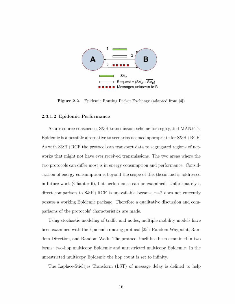
The transmitting node starts by sending a summary vector (bit vector) to
the receiving node (SVA in Figure 2.1), which is a hash table that is keyed by
the unique identifier and is [1 × P ] in size (where P is the number of packets
transmitted by any node). This summary vector describes to the receiving node
which packets the transmitting node is ready to send. The receiving node takes
the summary vector and performs the logical AND (∧) operation on the inverse of
its own summary vector (¬SVB in Figure 2.1), which informs the receiving node of
the packets that are available and not previously been transferred. The receiving
node then generates a request, which is answered by the the transmitting node.
This process is then repeated vice versa or as long as the nodes are in range.
Similar to the TTL field in IP, the hop count determines how many hops a
packet will travel before it is dropped. This value is set according to how much
node memory can be allocated for packet storage; the higher the hop count the
better the performance.
15
Figure 2.2. Epidemic Routing Packet Exchange (adapted from [4])
2.3.1.2 Epidemic Performance
As a resource conscience, S&H transmission scheme for segregated MANETs,
Epidemic is a possible alternative to scenarios deemed appropriate for S&H+RCF.
As with S&H+RCF the protocol can transport data to segregated regions of net-
works that might not have ever received transmissions. The two areas where the
two protocols can differ most is in energy consumption and performance. Consid-
eration of energy consumption is beyond the scope of this thesis and is addressed
in future work (Chapter 6), but performance can be examined. Unfortunately a
direct comparison to S&H+RCF is unavailable because ns-2 does not currently
possess a working Epidemic package. Therefore a qualitative discussion and com-
parisons of the protocols’ characteristics are made.
Using stochastic modeling of traffic and nodes, multiple mobility models have
been examined with the Epidemic routing protocol [25]: Random Waypoint, Ran-
dom Direction, and Random Walk. The protocol itself has been examined in two
forms: two-hop multicopy Epidemic and unrestricted multicopy Epidemic. In the
unrestricted multicopy Epidemic the hop count is set to infinity.
The Laplace-Stieltjes Transform (LST) of message delay is defined to help
16
normalize the results. In addition to the mathematical analysis, simulations were
run; both sets of results matched “very closely” [25]. Results differed based on
the form (unrestricted multicopy or two-hop multicopy) and mobility models com-
paring one another and determining the ponits of which performance was greatly
affected. Transmission range and the number of MANET nodes can be used to
describe performance in the network:
λ = O(r(N))
where λ is the inter-meeting time intensity and r(N) is the transmission range of
a network with N nodes [25].
Performance metrics of Epidemic routing have been examined: delivery delay,
loss probability, and power consumption [26]. MANETs consisting of N + 1 mo-
bile nodes using unrestricted multicopy Epidemic were in a closed area following
the random-waypoint and random-direction mobility models, with traffic gener-
ated according to a Poisson process. This analysis ascertains the basic network
characteristics of delay and loss, as well as captures the number of retransmissions
(used for calculating energy use) and storage requirements. Further analysis was
then done to extended models that included two-hop Epidemic, probablistic for-
warding, and limited-time forwarding. Finally, performance under limited buffer
size was analyzed with two drop schemes: drophead and droptail. The analysis
shows that Epidemic is intrinsically predictable and Markovian models can lead
to quite accurate performance predictions [26].
Epidemic routing under contention has also been examined [27]. Noting that
MANETs are often deployed in hostile environments, this research puts constraints
on bandwidth and scheduling while introducing signal interference.
17
2.3.2 Store and Haul
Store and Haul (S&H) is a paradigm that uses node mobility to physically
carry data across regions of MANETs where communication is not possible due
to connectivity limitations, interference, or eavesdropping. This label was first
coined in 2002 [3] and was first published in the Epidemic routing protocol two
years earlier [4]. S&H has been explored in a variety of ways and is sometimes
referred to as store and carry forward (SCF) or message ferrying [4], [7], [28], [5].
The interesting concept behind S&H is that it uses mobility to overcome some
of the challenges created by mobility itself. This essentially turns a potential
challenge into a potential strength and uniquely applicable to MANETs in need
of DTN architectures.
2.3.3 Message Ferrying and Store-Carry-Forward
Message Ferrying (MF) is a store-and-haul variant in which only predetermined
nodes can use their mobility to physically transport data through the MANET,
unlike Epidemic in which any node can carry data across the network [6]. There
are a wide variety of implementations, each with varying characteristics, objec-
tives, and results.
The intial implementation designates message ferries that have a determinis-
tic mobility model while the rest of the regular nodes may have stochastic node
mobility [5]. Ferries are classified as task-oriented or message-oriented. Task-
oriented ferries’ path is designed for other non-messaging reasons such as a bus
on a campus or planes patroling a battlefield. Message-oriented ferries follow tra-
jectories designed to enhance communications. Four message ferrying categories
are crisis-driven, geography-driven, cost-driven, and service-driven. Crisis-driven
18
applications include battlefield or disaster area communication, when infrastruc-
ture is unavailable due to environmental conditions. The ferries enable the segre-
gated areas to communicate with one another by transporting data between them.
Geography-driven types of network nodes are often densely deployed within clus-
ters but are inherently sparse due to larger geographic distances between the
clusters. In the cost-driven category, ferries can be used where it would be expen-
sive to create network infrastructure between clusters. This category includes city
buses that could transport non-critical or best-effort traffic to other networks. The
service-driven category is an opportunity for MF to provide a service not already
available in the existing network infrastructure, such as anonymous communica-
tion within a network [5].
Node-Initiated Message Ferrying (NIMF) is a scheme in which the ferry moves
along a predetermined route known by the regular nodes. Nodes are then respon-
sible for traveling to meet the ferry when needed. Conversely, the node needs
to periodically check to see if messages are waiting for delivery from the ferry.
Ferry-Initiated Message Ferrying (FIMF) uses the opposite initiation in which the
ferry travels to the nodes for communication. This can be accomplished either by
ferry nodes periodically traveling to all the regular nodes or by some sort of signal
or beacon the regular nodes produce when they are ready to communicate.
Node buffer sizes, both in the ferries and regular nodes, as well as the impacts
of node mobility and transmissions range affect performance. Multiple ferries can
work in tandem alleviating contention, with coordination of regular nodes and
ferries. The research is regarded as an in depth analysis of message ferrying uses
and concerns [5].
Other MF research goes delves deeper into different strategies, potential uses,
19
performance, and characteristics, including differentiated services [29], optimizing
ferry routes, scheduling ferries, and ferry buffer management [30, 6, 31]. There
are also have been proposals for more efficient or effective strategies [32, 30].
Store-Carry-Forward (SCF) is another term used for S&H and also been re-
ferred to as mobility-assisted routing [33] and store and foward [29]. Several pro-
tocols have been labeled as SCF. The following sections cover three of the most
common.
2.3.3.1 MeDeHa
An example of limited use of SCF can be found in the Message Delivery in
Heterogeneous, Disruption-prone Networks (MeDeHa) protocol [34]. The primary
objective of MeDeHa is establish a framework for data delivery in heterogeneous
DTNs. It establishes this with four functional components: message relaying,
buffering, topology and content information exchange, and traffic differentiation.
The first component, message relaying, is the SCF piece, that is a system in
which all nodes can store and haul data. It is referred to as simpler and more
opportunistic than other SCF systems: simple in that scheduling, beaconing, or
summoning systems are not needed and more opportunistic in that the nodes
can take advantage of more network types. Buffering is directly addressed for
two reasons. First in heterogeneous networks the Access Points (AP) or other
gateways between the varying kinds of networks are of great strategic value, and
should be used as a temporary repository for undelivered messages due to their
high availability of resources. This can be enhanced by buffering at the data link
layer [34].
The topology and content information exchange portion consists of nodes pe-
20
riodically exchanging a few key pieces of information: topology, routing table,
and message buffer information, as well as available resources and performance
metrics. The overhead in this is more than offset with the improvements in relay
selection. The last component of MeDeHa is traffic differentiation. Here MeDeHa
attempts to satisfy application-specific requirements, by using message priority,
TTL, scope, and message tags to provide quality-of-service (QoS) [34].
The basics of the node operation is shown in Figure 2.2. Each node has one of
four states: idle, receive, forward, and buffer. The nodes start in the idle state and
will switch to the forward state if it has a message to send, or will switch to the
receive state upon the reception of a message. After receiving a message the node
will either recognize itself as the destination and return to idle state or switch to
the forwarding state if it is not the destination. Once in the forwarding state it
will forward the message if an acceptable path or suitable relay is found. If not,
it switches to the buffered state. Here the node decides whether or not to drop
the message or store the message in the buffer for later attempts at transmission.
In either case, the node will return to the idle state.
In summary, MeDeHa uses a combination of networks to efficiently buffer
messages and carry them through areas where there is no network infrastructure
[34].
2.3.3.2 Efficient Adaptive Routing
Another example of the use of SCF is the Efficient Adaptive Routing (EAR)
protocol for DTN [35]. EAR is characterized as a bandwidth efficient solution that
achieves its efficiency by dynamically allocating available bandwidth according
to the current state of the DTN. The two components by which EAR conserves
21
Figure 2.3. MeDeHa State Diagram. Adapted from [34]
bandwidth are through multi-hop routing and mobility-assisted routing. The EAR
protocol uses multi-hop routing when it can to transmit data as it usually provides
the best performance. However if the network is congested or a path is not known,
EAR can limit the number of hops or switch to the second component: mobility-
assisted routing. Here the node carries the message to be delivered to a more
centralized location, one that is more likely to know the path or a location with
less congestion. EAR out performs DSDV in most scenarios, in both bandwidth
and PDR [35].
2.3.3.3 Store-and-Carry Forward Routing
Store-and-Carry Forward Routing (SCFR) spans the spectrum from connection-
based MANETs (networks lacking the capability of carrying data) to “mobility-
assisted” MANETs (such as S&H and SCF) [36]. SCFR is a complex MF protocol
that can be seen in the summation of the four main components of the strategy:
22
• design of ferry trajectory and rendezvous points
• movement scheduling for ferry and message
• role changing abilities amongst network nodes (as needed)
• node redistribution through ferry movement
One of the more notable characteristics of SCFR is the ability to effectively and
efficiently redistribute nodes throughout a geographic space. As seen in Figure
2.4, the nodes are spread out through the physical constraints of network while
keeping connectivity amongst all nodes. This is achieved through node adaptation
(switching back and forth from ferry to non-ferry) and dynamic reorganization.
Figure 2.4. Node Redistribution by SCFR. Adapted from [36]
The dual-control plane system divides node control into two planes for hetero-
geneous networks [37]: the Stationary-plane (S-plane) for message routing among
stationary nodes and the Mobility-plane (M-plane) for trajectory control of the
mobile nodes. In this system, all mobile nodes can act as ferries and transport
data, and nodes may change roles when it is necessary. Figure 2.5 shows the logical
separation between the planes. Through this system the network can efficiently
control node movement to keep partitioned networks connected [37].
23
Figure 2.5. Dual Control Planes for SCF. Adapted from [37]
2.3.4 VANETs
Vehicale Ad-Hoc Networks (VANETs) are a type of MANET that classifies
their nodes as “vehicles”, such as automobiles, trains, and buses. This implies
that the nodes are not only mobile but have ample power resources, transmission
range, and speed. This is in stark contrast to other types of MANETs, such as
wireless sensor networks and Personal Area Networks (PANs).
VANET research often uses the SCF mechanism and nomenclature and is
applicable to SCF due to the ample resources [38]. SCF has been proposed in
conjunction with vehicle navigation systems to connect sparsely communicated
VANETs. The routing methodology analyzes the vehicles vectors from tuples that
are shared amongst the vehicles to determine to which vehicle to forward data or
which direction data should be forwarded. The tuples contain vehicle destination,
waypoints, and street paths. In its simplest form this system can provide infor-
mation such as weather, road conditions, and traffic conditions. However, this
methodology could also be used to for inter-vehicle, end-to-end communication
such as messaging, sharing data, finding locations, and Internet access. These
services are described as Vehicle-to-Vehicle (V2V) or Vehicle-to-Roadside (V2R),
24
for which geography based routing can be used [38, 39].
Other work investigating the benefits of SCF and VANETs has evaluated per-
formance, using Markov chain models to evaluate SCF procedure in VANETs [39]
under varying network conditions with dynamically changing vehicle densities.
Markov chain modeling is especially applicable for analyzing mobility at an inter-
section, which is central to VANETs. It is important to the correct hop count to
increase the availability of information, while trying to keep traffic and congestion
to a minimum [39].
25
Chapter 3
Store-and-Haul with
Repeated Controlled Flooding
Store-and-Haul with Repeated Controlled Flooding (S&H+RCF) is an attempt
to alleviate some of the challenges inherent in a sparsely connected MANETs. The
protocol is described in this chapter first with a basic overview and impetus behind
the protocol in Section 3.1. The chapter then closes with a detailed description
of the protocol in Section 3.2.
3.1 Overview of S&H+RCF
S&H+RCF research began by evaluating basic kinds of connectionless com-
munication, namely controlled flooding – one of the most simple kinds of connec-
tionless communication. As previously mentioned, controlled flooding is defined
as transmitting data to all known communication paths regardless of whether or
not the recipient can be reached on a particular link [8]. Each node receiving
that transmission continues to forward the packet in the same manner except
26
back to the path from whence it came (Chapter 2.1). Controlled flooding was
deemed preferable for this research due its increased efficiency over regular flood-
ing. Furthermore, controlled flooding seemed suitable not only for its simplicity
but the potential synergy when shared with S&H. All the strategy lacked was the
repetition of the transmissions and delay for the topologies to change.
In most networks repeating flooded transmissions is a waste of bandwidth as
recipients have already received the flooded data due to static, contiguous topolo-
gies. But the dynamic topologies inherent in MANETs produce new links as time
changes. Additionally, partitions often arise and create pockets of unreachable
nodes. It is the characteristic of node mobility intrinsic to MANETs that makes
repeating floods advantageous. Naturally, the S&H movement is the linchpin that
augments the effectiveness of the controlled flooding and dynamic topologies by
bringing the transmissions to the unreachable nodes.
This repeated, controlled flooding (RCF) augmented with S&H is a novel,
yet simple solution for many different kinds of MANETs. From Personal Area
Networks (PANs) to sensor networks, this strategy could increase packet deliv-
ery ratios (PDRs) and extend communication coverage where normal MANETs
without S&H would not have communicated. Additionally, this strategy could be
modified for different kinds of MANETs. Performance could be enhanced simply
by increasing or decreasing the number of repeats. It could also be enhanced
by modifying the interval between repeats, depending upon the characteristics of
the MANETs in question. These modifications could even be made in real time
depending on the requirements of a particular scenario.
27
3.2 Mechanism Description
S&H+RCF communication operates in the following manner: when a node
has a message to send, it floods the message to all surrounding neighbors. The
neighbors then relay the message immediately to their neighbors, to achieve the
best possible performance equivalent to controlled flooding. The node then waits
a specified interval and then repeats the transmission. The node repeats this
process (waiting and retransmitting) until a specified number of transmissions is
met, as outlined in the flowchart found in Figure 3.1.
There is significant potential in the S&H methodology when combined with
RCF. The improvements chronicle which MANET characteristics combined with
which S&H+RCF settings yield desirable results. Improvement in packet delivery
is the main goal of the strategy.
Expectedly, the improvements do not come without a cost. The tradeoffs for
improved packet delivery ratio (PDR) through S&H+RCF are increased delays
and increased consumption of energy through additional retransmissions. Chal-
lenges the S&H+RCF mechanism would add to securing transmissions are outside
the scope of this research. The additional drains in energy are also mentioned in
Section 6.2.
28
Packet Already Recv?
Receive Packet
Start
Yes Drop Packet
Repeat transmission
(n -1)
n = 0 Drop Packet
Wait interval
(tD)
n = total number of transmissions
tD = time delay between transmissions
No
Yes
No
Stop
Stop
Addressed to this node?
Forward packet up the stack
StopYes
No
Figure 3.1. Flowchart of S&H+RCF
29
Chapter 4
Simulations
Due to the expense and difficulty of building and running actual MANETs,
simulations are the source of all data gathered in this thesis. The simulations are
run on the network simulator ns-2, a discrete event network simulator. Each net-
work event (e.g. node movement, transmission, error, collision) is chronologically
recorded into a trace file, as the simulation progresses. Calculations were made
from the data collected and conclusions were then drawn from those calculations.
The standard ns-2 distribution does not have the capability to simulate S&H
networks. The simulation software had to be customized so that the simulated
nodes would carry data and transmit that data at the appropriate time. After
the ns-2 software was modified, it had to be tested thoroughly. Starting first with
simple examples and working to complex simulations, the modified version was
always checked for inconsistencies and mistakes. Once the modified version was
verified through extensive testing, the network models were designed. The goal
of the model design was to be as realistic as possible. Furthermore, the scenarios
in which those models were simulated were also designed based on realistic net-
work conditions and realistic node capabilities. Finally, some of the limitations
30
of the software and hardware resource constraints were overcome through design
refinement and adjustments in both the models and scenarios.
The chapter is organized as follows: Section 4.1 describes the changes made
to the ns-2 software, Section 4.2 outlines the static network parameters found
in all the simulations, Section 4.3 explains the network scenarios in which the
simulations were run, and Section 4.4 ends the chapter by explaining how results
were verified.
4.1 Modifications to ns-2
An ns-2 distribution can be modified by editing the C++ source code. The
modified code is then recompiled after editing and executed for the desired sim-
ulation. As with many software suites programmed in C++, editing source code
can be a very complex process; there are many C++ source and header files and
finding the right files to modify can be quite challenging.
The most current version of ns-2 at the time this thesis was started was ns-
2.31. This distribution provided all files that were modified and generated all
the simulations. After close inspection of the available files, modifying an existing
routing protocol would be the best way to produced the desired effect. The closest
standard routing protocol included in ns-2.31 is the flooding protocol – used to
produce uncontrolled flooding [40]. Each routing protocol had a header file and
a source file. These two files were used as a template to create the ResiliNets
Flooding protocol.
The first modifications were designed to make the flooding controlled. In the
native ns-2 flooding protocol all packets were passed up through the layers once
they were received. To make the flooding controlled, packets already received by
31
the node should be dropped as soon as possible. This means that all the packets
received must be tracked in some kind of data structure. This is accomplished by
taking the packet ID and asserting a bit in a bit array indexed by the packet ID,
such that every received packet would first check an array for a previous instance.
If the bit in the array with the value of the packet ID had been asserted, then the
node had seen the packet before and the packet should immediately be dropped;
the drop occurs at layer 2 [41].
After controlled flooding was established the next step was to create repeated
controlled flooding. C++ structures were created to hold the packet ID, destina-
tion IP addresses, number times to be repeated, and interval time. From this a
separate scheduling method creates the appropriate packets and schedules them
for transmission within the node, producing RCF [42].
When the new packets are created so they can be repeated, they are created
with the same packet ID and destination IP address. The payload is simply
filler information and irrelevant to the experiment (except for the size needed for
performance analysis). The process of creating RCF also provides the desired
S&H mechanism, since packets are held while the nodes are moving.
4.2 Simulation Model
Once ns-2 was modified to incorporate S&H+RCF, the simulation models
were designed. First, the physical topology was established, with randomly placed
nodes in a 1000 meter square. All the nodes are mobile and able to S&H data. The
antenna transmitted omni-directionally and the IEEE 802.11 wireless protocol is
chosen for its familiarity and popularity. Thirty nodes are used in all simulations
and the queue length is set to 50 packets for each node. The simulations run for
32
1000 seconds. Finally, the bandwidth on every node is set to 54 Mb/s and the
random-waypoint (RWP) mobility model is used for node movement with speeds
randomly selected between 10 and 20 m/s. All of these settings remained con-
sistent throughout all simulations. The static parameters used in the simulations
are shown in Table 4.1.
Table 4.1. Simulation Parameters
Parameter ValueRouting S&H+RCFArea 1000× 1000Number of nodes 30Simulation time 1000 [s]Link layer LLMAC type 802.11Mobility model Random WaypointBandwidth 54 Mb/sAntenna OmniQueue length 50 packetsChannel type WirelessRadio propagation TwoRayGroundNode speed 10 m/s - 20 m/s
Speed and paths are set parameters of the simulation movement files. The
movement files instruct the nodes when to move, where to move to, and how fast
to travel. Partitions are created when node density is low enough that adjusting
the transmission range causes parts of the network to become disconnected. Using
Perl scripts, the number of partitions is calculated by finding the running average
from the movement files. The movement files are repeatedly generated until the
desired running average is achieved.
Traffic is created through Constant Bit Rate (CBR) generators on ten ran-
domly selected nodes. Ten other randomly selected nodes are chosen to receive
the traffic generated. The total amount of packets created in each scenario was
33
50,000. The packets are 1 KB in size. Five packets are transmitted every second,
per transmitting node, which results in a bandwidth of 40 Kb/s.
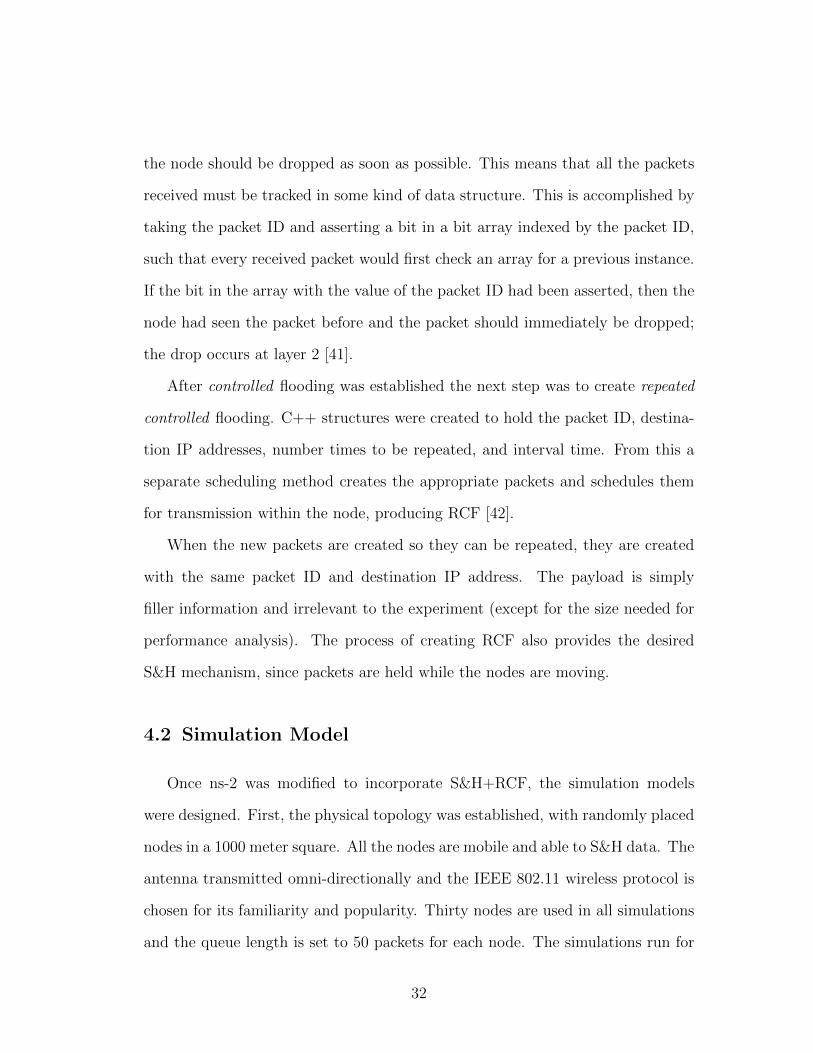
4.3 Simulation Scenarios
Several different scenarios involving S&H+RCF are examined, with the num-
ber of transmissions and the intervals between those transmissions varied in dif-
ferent combinations. Three options for the number of transmissions are used: one,
two, three, and five total transmissions (by a node for each packet received).
Initially, the intervals between transmissions were only three values: one sec-
ond, three seconds, and five seconds, however, longer intervals were needed to
explore performance tradeoffs – resulting in scenarios with 10, 20, 40, and 60
second intervals. Unfortunately, when intervals were longer than ten seconds the
server ran out of available memory. Solutions were sought to create simulated
scenarios with intervals larger than ten seconds. It was determined that larger
intervals could be artificially created within memory constraints by increasing the
node speed, the premise being that nodes would move faster, essentially speeding
up time, and creating a larger, artificial interval. Testing began with two sets
of scenarios created with ten second intervals: one set at ten seconds and nodes
moving at normal speeds and one scenario set with five seconds and nodes mov-
ing twice as fast; everything being exactly the same, except the interval between
transmissions and the node speed. Comparatively, the artificially created inter-
val of ten seconds produces results within ± 7% of the PDR values created by
simulations with natively set intervals of ten seconds, as illustrated in Figure 4.1.
Unfortunately, the delay values are several degrees of magnitude off from the na-
tively created ones. The delay is much smaller in the artifically created intervals
34
PD
R [%
]
partitions
∆t=10s∆t=10s*
0.0
0.1
0.2
0.3
0.4
0.5
0.6
0.7
0.8
0.9
1.0
0.0 2.0 4.0 6.0 8.0 10.0 12.0
Figure 4.1. Difference between natively set and artificially set in-tervals (∆t)
than the natively created intervals because the nodes are moving much faster and
disseminating the messages with less delay.
While artificially creating intervals is not preferred, there is still value and
insight to be gained from examining those results. Table 3.2 shows all the com-
binations used in number of transmissions and interval between transmissions.
All interval values marked with an asterisk signify artificial creation by increasing
node speed.
The final network factor simulated is the number of partitions. This is nec-
essary to test the efficacy of S&H+RCF in partitioned networks. Partitions re-
sult from sparse connectivity by reducing the transmission range of the networks
nodes. All 30 nodes in the simulations have the same transmission ranges. The
average number of partitions are calculated from the movement files, as previously
Finally, each scenario was run at least three times each to increase confidence
in the results.
4.4 Functional Verification
The results of the simulations are repeatedly verified for accuracy. The ver-
ification initially began by creating test simulations that are very small. Two
packets are transmitted in a network of only three nodes. Each discrete event
is then examined for functional accuracy from within the simulation trace files.
The tests are then increased in size and complexity, each test ending with an
examination for functional accuracy. Once the tests reached ten nodes with 100
transmitted packets and functional accuracy is maintained, the simulations show
they reliably scale to larger networks.
There are also internal verification processes within the analysis of all the trace
files. Perl scripts are run on all the trace files to look for unexplained anomalies.
36
The Perl scripts count how many packets are sent and how many packets are
received to ensure that there are never any instances of more received packets
than packets sent. The Perl scripts also check received times to ensure no packets
are received before they are sent. Finally, there are random audits of the trace
files to provide additional quality assurance; random snippets of randomly chosen
trace files were examined to verify functional accuracy.
37
Chapter 5
Analysis
This chapter presents the analysis of the S&H+RCF simulations runs. Each
scenario is run three times using ns-2 and all the trace files are collected for
parsing and data extraction. Perl scripts are used to analyze these trace files.
The Perl scripts not only extract the necessary data, they calculate the desired
values and averages, while looking for potential errors by doing consistency checks
on the data (as discussed in Section 4.4). Many of these values are considered
pertinent and recorded in a spreadsheet, the most noteworthy of which are the
number of packets successfully received by the nodes and the delay incurred by
each successful reception. Those packets successfully received are used to calculate
the scenario’s packet delivery ratio (PDR). The delay incurred by each successful
reception is used to calculate the average end-to-end (E2E) delay in the scenario.
The other noteworthy values extracted from the ns-2 files are the average node
degree, average number of partitions, and average goodput.
The simulations have three variable parameters: average number of partitions
in the scenario (or network density), number of transmissions for each packet, and
the time interval each node waits between transmissions. These three variables
38
change from scenario to scenario while all other network parameters remained
static. These variables are listed in Table 5.1 along with their possible values.
Table 5.1. Possible Dynamic Variable ValuesVariable Description Possible Valuesn Number of transmissions (total) 2 tx, 3 tx, 5 tx∆t Interval between transmissions 1 s, 3 s, 5 s, 10 s,
20 s, 40 s, 60 sP Avg. number of partitions Contiguous network (1 part),
2 part, 3 part, 5 part, 8 part,10 part, 12 part
From all these values recorded in a spreadsheet, tables are created and plotted
using Gnuplot to help provide for the analysis of S&H+RCF.
This chapter is organized to examine the results in three different ways: with
respect to network density (Section 5.1), the interval between transmissions (Sec-
tion 5.2), and the quantity of repeats (5.3). Each section has two subsections:
one subsection examines the PDR (packet delivery ratio) results while the other
subsection focuses on the delay results.
5.1 Analysis of Network Density
The first part of the analysis focuses on average network density or average
number of partitions – network density is simply the concentration of nodes in a
given area and the number or partitions is the number or segregated groups of
nodes such that they are out range and unable to communicate with each other.
Density is examined in relation to the other two dynamic variables, with network
density values plotted along the x-axis. Thus there is a set of plots where the
interval between transmissions is changed and the quantity of transmissions are
held constant, and a second set of plots keep the interval between transmissions
39
held constant while the quantity of transmissions are changed. This is done for
both PDR and delay.
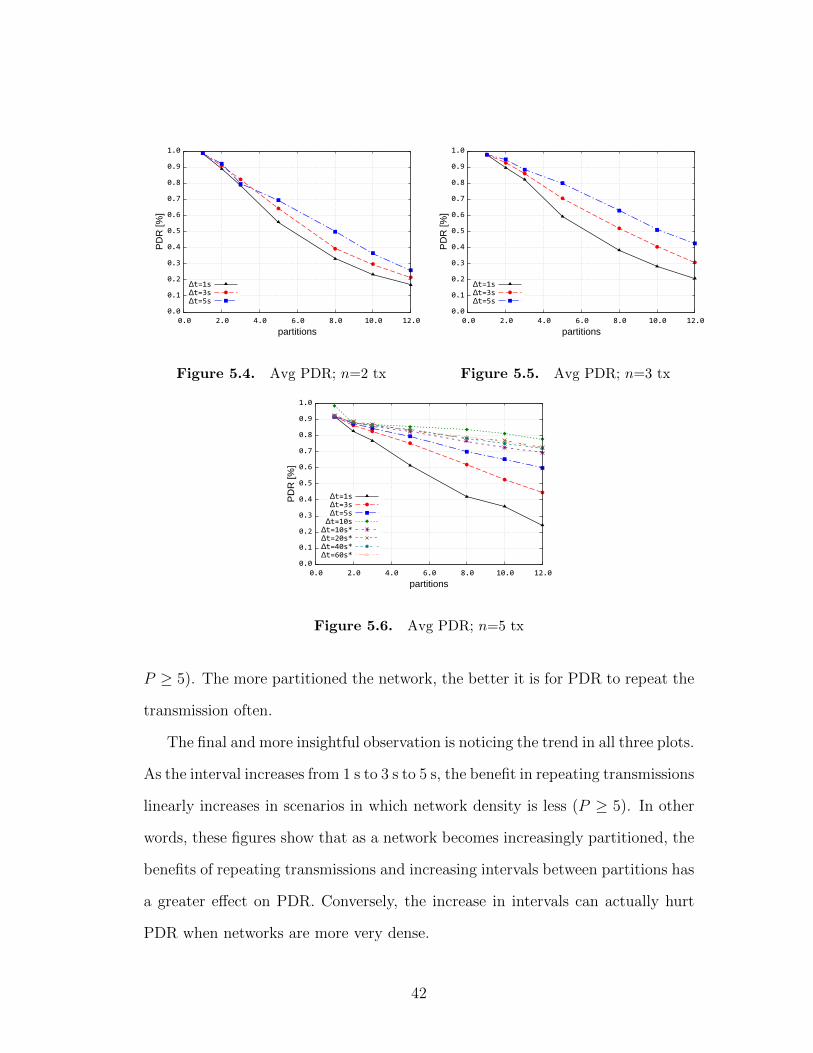
5.1.1 Effect of Network Density on PDR
This section analyzes the effect of varying the network density on PDR, as
measured by the number of partitions. This is done for a variety of transmission
repeat parameters. The first three plots, Figure 5.1, Figure 5.2, and Figure 5.3
have similar, consistent traits. Most notable is how the PDR decreases as the
network becomes more partitioned. This is to be expected and it can be fur-
ther asserted that as partitions reach the number of nodes in the network for all
scenarios, PDR is reduced to zero – expressed by the following equation:
limP→n
PDR→ 0
In these three plots the control data from ordinary controlled flooding (as
opposed to RCF) can be seen where n=1 tx. Those control simulations only
transmit once and thus the interval value is meaningless. Controlled flooding (CF)
had higher PDR values in very dense simulations, but performed poorly when the
networks were less dense. The real benefits of repetitions can be seen as the
network density decreases (as P → 12). Figures 5.2 and 5.3 show how increasing
the interval between transmissions (∆t) increases the PDR dramatically.
Another characteristic seen in these figures is how ∆t = 5 s (Figure 5.3) sce-
narios outperform the ∆t = 2 s plots (Figure 5.2) in overall aggregate PDR and
the ∆t = 3 s plots outperform the ∆t = 1 s (Figure 5.1) plots in overall aggregate
PDR. The longer the interval between transmissions, the higher the PDR when
the number of transmissions is the same.
40
PD
R [%
]
partitions
n=1tx
n=2tx
n=3tx
n=5tx
0.0
0.1
0.2
0.3
0.4
0.5
0.6
0.7
0.8
0.9
1.0
0.0 2.0 4.0 6.0 8.0 10.0 12.0
Figure 5.1. Avg PDR; ∆t=1 s
PD
R [%
]
partitions
n=1tx
n=2tx
n=3tx
n=5tx
0.0
0.1
0.2
0.3
0.4
0.5
0.6
0.7
0.8
0.9
1.0
0.0 2.0 4.0 6.0 8.0 10.0 12.0
Figure 5.2. Avg PDR; ∆t=3 s
PD
R [%
]
partitions
n=1tx
n=2tx
n=3tx
n=5tx
0.0
0.1
0.2
0.3
0.4
0.5
0.6
0.7
0.8
0.9
1.0
0.0 2.0 4.0 6.0 8.0 10.0 12.0
Figure 5.3. Avg PDR; ∆t=5 s
While the PDR increase from increased interval between transmissions (∆t) is
notable, a more intriguing observation is where the plots in each figure intersect.
This shows when the benefit of the increased transmissions begins to take effect
as a network is further segregated. It also shows that when a network is very
dense, the extra transmissions are superfluous and result in more interference.
Consequently, this decreases PDR for scenarios in which the network is very dense
and the number of transmissions is high. However, the more partitioned networks
show increases in PDR when transmissions and intervals are increase (e.g. the n=
5 tx start to significantly outperform the n= 2 tx and n= 3 tx scenarios in which
41
PD
R [%
]
partitions
∆t=1s∆t=3s∆t=5s
0.0
0.1
0.2
0.3
0.4
0.5
0.6
0.7
0.8
0.9
1.0
0.0 2.0 4.0 6.0 8.0 10.0 12.0
Figure 5.4. Avg PDR; n=2 tx
PD
R [%
]
partitions
∆t=1s∆t=3s∆t=5s
0.0
0.1
0.2
0.3
0.4
0.5
0.6
0.7
0.8
0.9
1.0
0.0 2.0 4.0 6.0 8.0 10.0 12.0
Figure 5.5. Avg PDR; n=3 tx
PD
R [%
]
partitions
∆t=1s∆t=3s∆t=5s
∆t=10s∆t=10s*∆t=20s*∆t=40s*∆t=60s*
0.0
0.1
0.2
0.3
0.4
0.5
0.6
0.7
0.8
0.9
1.0
0.0 2.0 4.0 6.0 8.0 10.0 12.0
Figure 5.6. Avg PDR; n=5 tx
P ≥ 5). The more partitioned the network, the better it is for PDR to repeat the
transmission often.
The final and more insightful observation is noticing the trend in all three plots.
As the interval increases from 1 s to 3 s to 5 s, the benefit in repeating transmissions
linearly increases in scenarios in which network density is less (P ≥ 5). In other
words, these figures show that as a network becomes increasingly partitioned, the
benefits of repeating transmissions and increasing intervals between partitions has
a greater effect on PDR. Conversely, the increase in intervals can actually hurt
PDR when networks are more very dense.
42
The second set of scenarios analyzed are those in which the number of trans-
missions remains static while the intervals between transmissions vary. As with
the first family of plots, these have similar and consistent traits. The PDR de-
creases as the network becomes more and more partitioned. The deficiency in
which too many transmissions can have negative affect on PDR is shown again in
Figures 5.4, 5.5, and 5.6. However because Figure 5.6 shows extended intervals
between transmissions (some of which are artificially created)1, it has additional
information to offer.
Figure 5.6 shows that as the interval between transmissions becomes large
enough, the loss in PDR in dense networks can be mitigated. The congestion and
collisions experienced from heavy transmissions can be offset with large intervals
between transmissions. It also shows a diminishing return in PDR from increasing
the interval past a certain value. In these experiments that value was ∆t =10 s.
The cause of this diminishing return is from nodes moving out of range before
other nodes actually transmit the data, essentially missing their opportunity, or
“window” to transmit. In other words, nodes move in and out of range all before
a transmitting node has a chance to repeat the transmission.
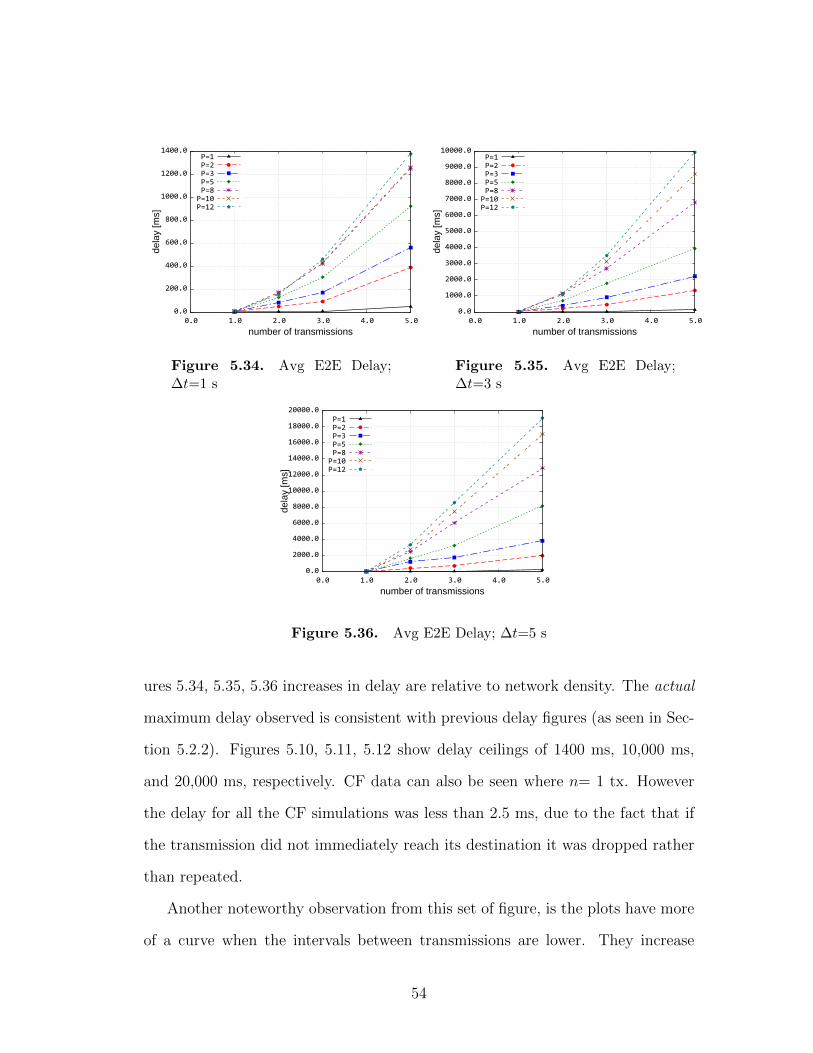
5.1.2 Effect of Network Density on Delay
Along with PDR, delay is a very important network characteristic. E2E (End
to End) delay is defined as the amount of time it takes for a packet to reach its
destination after transmission. All of delay values are summed together to provide
the average E2E delay of each scenario. This delay in communication is often the
1Some experimental scenarios with increases of interval between transmissions were tried.They only make it into select figures because only PDR values were accurately given and oftendo not relate to other scenarios, as discussed in Section 4.3
43
dela
y [m
s]
partitions
n=1tx
n=2tx
n=3tx
n=5tx
0.0
200.0
400.0
600.0
800.0
1000.0
1200.0
1400.0
0.0 2.0 4.0 6.0 8.0 10.0 12.0
Figure 5.7. Avg E2E Delay;∆t=1 s
dela
y [m
s]
partitions
n=1tx
n=2tx
n=3tx
n=5tx
0.0
1000.0
2000.0
3000.0
4000.0
5000.0
6000.0
7000.0
8000.0
9000.0
10000.0
0.0 2.0 4.0 6.0 8.0 10.0 12.0
Figure 5.8. Avg E2E Delay;∆t=3 s
dela
y [m
s]
partitions
n=1tx
n=2tx
n=3tx
n=5tx
0.0
2000.0
4000.0
6000.0
8000.0
10000.0
12000.0
14000.0
16000.0
18000.0
20000.0
0.0 2.0 4.0 6.0 8.0 10.0 12.0
Figure 5.9. Avg E2E Delay; ∆t=5 s
trade off for increased PDR in MANETs. There are many cases where delay is
the by-product of increasing successfully received transmissions ([4], [5], [6], [29],
[11]). S&H+RCF also experiences delays as a cost of increasing PDR. However,
those delays are increased only for the packets that would not have been received
in regular CF; E2E delays are never worse in S&H+RCF than CF. S&H+RCF
subscribes to the philosophy in DTNs – a successful, albeit delayed, transmission
is “better late than never”.
The first set of scenarios analyzed are those in which the interval between
transmission remains static while the number of partitions and transmissions are
44
dela
y [m
s]
partitions
∆t=1s∆t=3s∆t=5s
0.0
500.0
1000.0
1500.0
2000.0
2500.0
3000.0
3500.0
0.0 2.0 4.0 6.0 8.0 10.0 12.0
Figure 5.10. Avg E2E Delay;n=2 tx
dela
y [m
s]
partitions
∆t=1s∆t=3s∆t=5s
0.0
1000.0
2000.0
3000.0
4000.0
5000.0
6000.0
7000.0
8000.0
9000.0
0.0 2.0 4.0 6.0 8.0 10.0 12.0
Figure 5.11. Avg E2E Delay;n=3 tx
dela
y [m
s]
partitions
∆t=1s∆t=3s∆t=5s
∆t=10s∆t=10s*∆t=20s*∆t=40s*∆t=60s*
0.0
5000.0
10000.0
15000.0
20000.0
25000.0
30000.0
35000.0
40000.0
45000.0
50000.0
0.0 2.0 4.0 6.0 8.0 10.0 12.0
Figure 5.12. Average E2E Delay; n=5 tx
varied. Here it can be seen in Figures 5.7, 5.8, and 5.9 that the delay increases
as the networks are more partitioned. It can also be seen how delay increases
as the number of transmissions increase. Additionally, the three plots show how
the CF simulations have a delay nearly equal 0 ms. This is due to the imme-
diate transmission of packets upon reception. While the delay is extremely low
and plateaus around 2.5 ms, it offset by extremely low PDR levels for highly
partitioned networks.
The quantity of the delay between the different figures is very pertinent. The
maximum amount of delay is a product of how many hops are taken before reach-
45
ing a destination – how many times it has to be repeated to make the next hop,
and how long of interval between each repeat. The maximum amount of delay, or
DMax, is
DMax = N×∆t× n
where N is the total number of nodes in the network, d is the E2E delay, and n
is the number of transmissions.
The maximum delay seen in the graphs varies depending on which value is set
in the interval between transmissions. In Figure 5.7 the delay never exceeds over
1400 ms. In Figure 5.8 the delay peaks at 10,000 ms and around 20,000 ms in
Figure 5.9. It is an exponential increase as the networks decrease in density and
increase in intervals between transmissions.
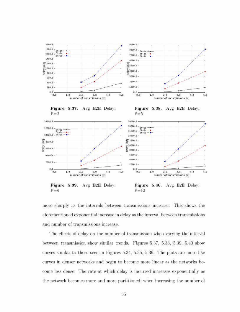
The second set of scenarios analyzed are those in which the number of trans-
missions remains static and the intervals between transmission are varied. As with
the earlier delay figures, Figures 5.10, 5.11, 5.12 demonstrate how delay increases
as the partitions increase and as the interval between transmissions increases. It is
notable to show how the maximum delay seen in Figures 5.10, 5.11, 5.12 is consis-
tent with those found in Figures 5.7, 5.8, 5.9 respectively. Variations in intervals
between transmission have about the same effect on delay as the variations in the
number of transmissions, which is consistent with
O(d) = N×∆t× n
It is also seen in Figure 5.9 in which the artificially created intervals do not
give accurate results in delay; most pronounced and clear when comparing ∆t
=10 s and ∆t =10 s*.
46
5.2 Analysis of Transmission Interval
The second part of the analysis examines the scenarios with respect to the
interval between transmissions, or ∆t. The figures place ∆t on the x-axis for a
variety of network densities and numbers of transmissions. The first subsection
pertains to the effect these variables have on PDR, while the following subsection
focuses on the effect they have on delay.
5.2.1 Effect of Repeat Interval on PDR
When examining the effect network density and transmission quantity have on
the interval between transmission, trends are established. The first set of Figures
5.13, 5.14, 5.15 show how PDR is more drastically and positively affected in the
more heavily partitioned networks. It is in those scenarios (P ≥ 5) in which
PDR is positively and greatly effected by an increase in the interval between
transmissions.
In Figures 5.16, 5.17, 5.18, 5.19, the PDR showing the greatest improvement
in increasing the number of transmissions is when the network is less dense. This
can be seen when comparing the more heavily partitioned scenarios (Figures 5.18
and 5.19) with the less partitioned, more dense scenarios (Figures 5.16 and 5.17).
In that direct comparison, the increased affect the number of transmissions has on
the interval between transmission has when the number of partitions are higher.
An interesting observation is seen in Figure 5.16. The n=3 tx plot begins to
outperform the n= 2 tx plot as the interval between transmissions increases. This
supports the assertion that congestion and collisions experienced when transmis-
sions are high and the network is dense can be mitigated with increased intervals
between transmissions. This does come at the cost of additional delay, as ex-
47
PD
R [%
]
interval between transmissions [s]
P=1
P=2
P=3
P=5
P=8
P=10
P=12
0.0
0.1
0.2
0.3
0.4
0.5
0.6
0.7
0.8
0.9
1.0
0.0 1.0 2.0 3.0 4.0 5.0
Figure 5.13. Avg PDR; n=2 tx
PD
R [%
]
interval between transmissions [s]
P=1
P=2
P=3
P=5
P=8
P=10
P=12
0.0
0.1
0.2
0.3
0.4
0.5
0.6
0.7
0.8
0.9
1.0
0.0 1.0 2.0 3.0 4.0 5.0
Figure 5.14. Avg PDR; n=3 tx
PD
R [%
]
interval between transmissions [s]
P=1
P=2
P=3
P=5
P=8
P=10
P=12
0.0
0.1
0.2
0.3
0.4
0.5
0.6
0.7
0.8
0.9
1.0
0.0 1.0 2.0 3.0 4.0 5.0
Figure 5.15. Avg PDR; n=5 tx
plained further in the following section.
5.2.2 Effect of Repeat Interval on Delay
The effect of network density and transmission quantity, with respect to the
interval between transmissions, is shown in two sets of figures.
Figures 5.20, 5.21, 5.22 show the increase in delay interval between transmis-
sions increase and network density decreases. The plots are less linear when n=
2 tx (Figure 5.20) and more linear in scenarios with more transmissions, as seen
in Figure 5.22. This suggests the exponential increase in delay as the interval
48
PD
R [%
]
interval between transmissions [s]
n=2tx
n=3tx
n=5tx
0.0
0.1
0.2
0.3
0.4
0.5
0.6
0.7
0.8
0.9
1.0
0.0 1.0 2.0 3.0 4.0 5.0
Figure 5.16. Avg PDR; P=2
PD
R [%
]
interval between transmissions [s]
n=2tx
n=3tx
n=5tx0.0
0.1
0.2
0.3
0.4
0.5
0.6
0.7
0.8
0.9
1.0
0.0 1.0 2.0 3.0 4.0 5.0
Figure 5.17. Avg PDR; P=5
PD
R [%
]
interval between transmissions [s]
n=2tx
n=3tx
n=5tx
0.0
0.1
0.2
0.3
0.4
0.5
0.6
0.7
0.8
0.9
1.0
0.0 1.0 2.0 3.0 4.0 5.0
Figure 5.18. Avg PDR; P=8
PD
R [%
]
interval between transmissions [s]
n=2tx
n=3tx
n=5tx0.0
0.1
0.2
0.3
0.4
0.5
0.6
0.7
0.8
0.9
1.0
0.0 1.0 2.0 3.0 4.0 5.0
Figure 5.19. Avg PDR; P=12
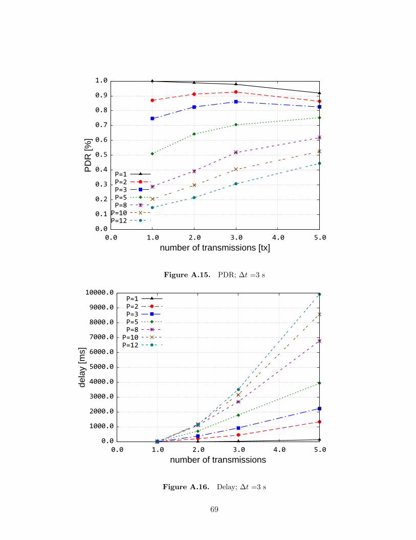
between transmissions and number of transmissions increase.
The trends established in the second set of figures once again show a similar
maximum in actual delay and show the exponential increase when both the in-
terval between transmissions are increased and network density decreased. These
characteristics are seen in Figures 5.23, 5.24, 5.25, 5.26.
5.3 Analysis of Transmission Quantity
The last part of the analysis examines the effect transmission quantity (the
number of transmissions n) has when varying the other two dynamic variables.
49
dela
y [m
s]
interval between transmissions [s]
P=1
P=2
P=3
P=5
P=8
P=10
P=12
0.0
500.0
1000.0
1500.0
2000.0
2500.0
3000.0
3500.0
0.0 1.0 2.0 3.0 4.0 5.0
Figure 5.20. Avg E2E Delay;n=2 tx
dela
y [m
s]
interval between transmissions [s]
P=1
P=2
P=3
P=5
P=8
P=10
P=12
0.0
1000.0
2000.0
3000.0
4000.0
5000.0
6000.0
7000.0
8000.0
9000.0
0.0 1.0 2.0 3.0 4.0 5.0
Figure 5.21. Avg E2E Delay;n=3 tx
dela
y [m
s]
interval between transmissions [s]
P=1
P=2
P=3
P=5
P=8
P=10
P=12
0.0
2000.0
4000.0
6000.0
8000.0
10000.0
12000.0
14000.0
16000.0
18000.0
20000.0
0.0 1.0 2.0 3.0 4.0 5.0
Figure 5.22. Avg E2E Delay; n=5 tx
In these sets of figures, the number of transmissions is displayed on the x-axis.
Two sets of figures are displayed: one set showing how network density affects
the characteristics of transmission quantity n and the other showing how interval
between transmissions ∆t affects transmission quantity. This is done for both
PDR and delay.
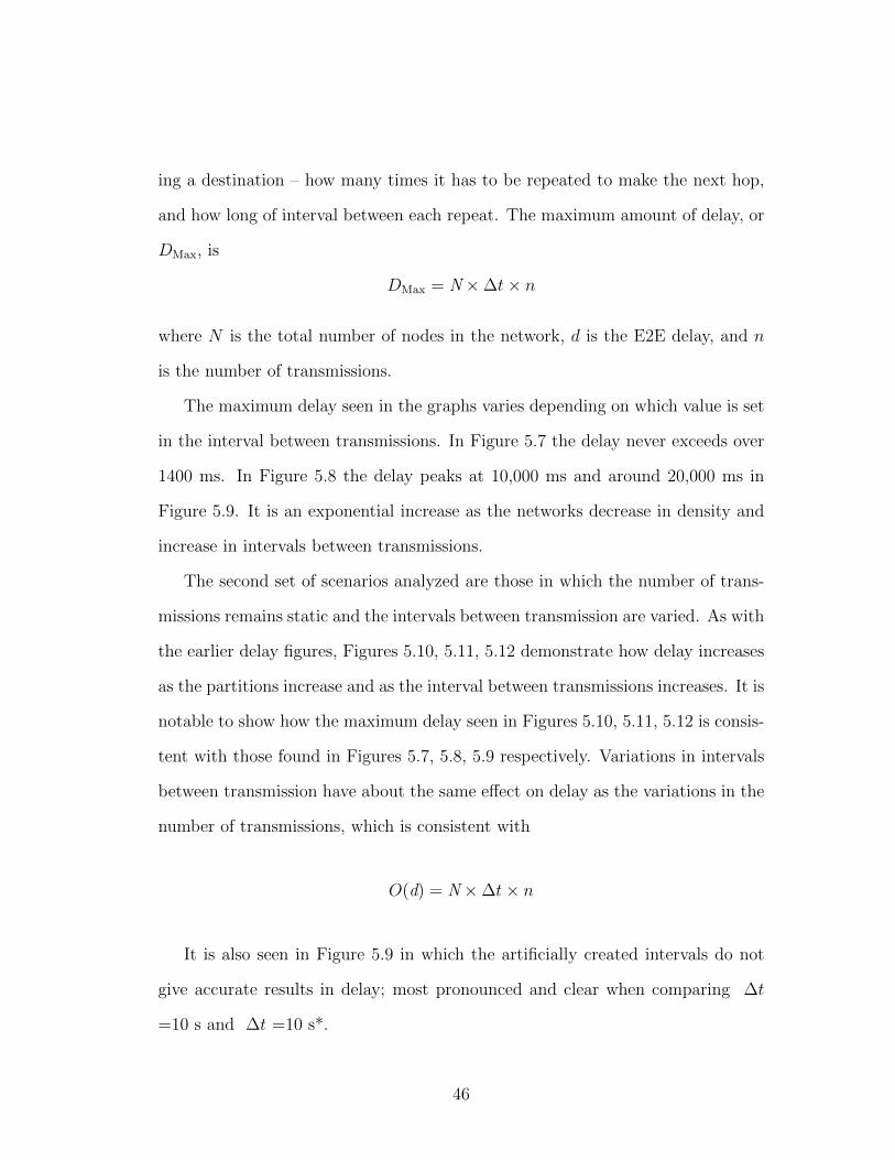
5.3.1 Effect of Transmission Repeats on PDR
In Figures 5.27, 5.28, 5.29 the number of transmissions affects the PDR in
one of two ways depending on what level of network density is examined. When
50
dela
y [m
s]
interval between transmissions [s]
n=2tx
n=3tx
n=5tx
0.0
200.0
400.0
600.0
800.0
1000.0
1200.0
1400.0
1600.0
1800.0
2000.0
0.0 1.0 2.0 3.0 4.0 5.0
Figure 5.23. Avg E2E Delay;P=2
dela
y [m
s]
interval between transmissions [s]
n=2tx
n=3tx
n=5tx
0.0
1000.0
2000.0
3000.0
4000.0
5000.0
6000.0
7000.0
8000.0
9000.0
0.0 1.0 2.0 3.0 4.0 5.0
Figure 5.24. Avg E2E Delay;P=5
dela
y [m
s]
interval between transmissions [s]
n=2tx
n=3tx
n=5tx
0.0
2000.0
4000.0
6000.0
8000.0
10000.0
12000.0
14000.0
0.0 1.0 2.0 3.0 4.0 5.0
Figure 5.25. Avg E2E Delay;P=8
dela
y [m
s]
interval between transmissions [s]
n=2tx
n=3tx
n=5tx
0.0
2000.0
4000.0
6000.0
8000.0
10000.0
12000.0
14000.0
16000.0
18000.0
20000.0
0.0 1.0 2.0 3.0 4.0 5.0
Figure 5.26. Avg E2E Delay;P=12
the network is relatively dense (P < 5), the increase in transmissions brings the
PDR down. Again, this is due to the congestion and collisions. However, as
the network becomes less dense (P ≥ 5), the increase in repeated transmissions
actually increases the PDR. This is seen across all three figures for all three values
of ∆t. Also seen across all three figures is how the increase in ∆t helps mitigate
the congestion and collisions in more dense networks. This can be seen in how
the plots converge at higher and higher levels of PDR as ∆t is increased.
The plots do not show the control data (CF simulations), for when n=1 tx,
because CF does not have a value for ∆t and could not be plotted. The plots
51
PD
R [%
]
number of transmissions [tx]
P=1
P=2
P=3
P=5
P=8
P=10
P=12
0.0
0.1
0.2
0.3
0.4
0.5
0.6
0.7
0.8
0.9
1.0
0.0 1.0 2.0 3.0 4.0 5.0
Figure 5.27. Avg PDR; ∆t=1 s
PD
R [%
]
number of transmissions [tx]
P=1
P=2
P=3
P=5
P=8
P=10
P=12
0.0
0.1
0.2
0.3
0.4
0.5
0.6
0.7
0.8
0.9
1.0
0.0 1.0 2.0 3.0 4.0 5.0
Figure 5.28. Avg PDR; ∆t=3 s
PD
R [%
]
number of transmissions [tx]
P=1
P=2
P=3
P=5
P=8
P=10
P=12
0.0
0.1
0.2
0.3
0.4
0.5
0.6
0.7
0.8
0.9
1.0
0.0 1.0 2.0 3.0 4.0 5.0
Figure 5.29. Avg PDR; ∆t=5 s
once again show how PDR increases immediately after the first partition or P ≥ 2.
This can be seen in the positive slopes between n= 1 and n= 2 for all plots where
P ≥ 2.
The second set of PDR plots shows four plots (selected from a family of seven
plots) that characterize PDR when partitions are kept static and interval between
transmissions are evaluated. They are shown in Figures 5.30, 5.31, 5.32, 5.33. In
this set of plots, the PDR is increasingly affected as the networks become more
and more partitioned – there is more of a disparity in the results of changing the
interval between transmissions as the networks become less dense. Most notably,
52
PD
R [%
]
number of transmissions [tx]
∆t=1s∆t=3s∆t=5s
0.0
0.1
0.2
0.3
0.4
0.5
0.6
0.7
0.8
0.9
1.0
0.0 1.0 2.0 3.0 4.0 5.0
Figure 5.30. Avg PDR; P=2
PD
R [%
]
number of transmissions [tx]
∆t=1s∆t=3s∆t=5s
0.0
0.1
0.2
0.3
0.4
0.5
0.6
0.7
0.8
0.9
1.0
0.0 1.0 2.0 3.0 4.0 5.0
Figure 5.31. Avg PDR; P=5
PD
R [%
]
number of transmissions [tx]
∆t=1s∆t=3s∆t=5s
0.0
0.1
0.2
0.3
0.4
0.5
0.6
0.7
0.8
0.9
1.0
0.0 1.0 2.0 3.0 4.0 5.0
Figure 5.32. Avg PDR; P=8
PD
R [%
]
number of transmissions [tx]
∆t=1s∆t=3s∆t=5s
0.0
0.1
0.2
0.3
0.4
0.5
0.6
0.7
0.8
0.9
1.0
0.0 1.0 2.0 3.0 4.0 5.0
Figure 5.33. Avg PDR; P=12
this can be seen when comparing Figure 5.30 to Figures 5.32 and 5.33. In this
comparison, it can be seen how the PDR values are very close to one another when
the network is more dense (Figure 5.30) and there is more of an effect on PDR,
when varying the interval between transmissions, in less dense networks (Figures
5.32 and 5.33).
5.3.2 Effect of Transmission Repeats on Delay
The figures showing the effect network density has on delay, when examining
the number of transmissions, stay consistent with previous observations. In Fig-
53
dela
y [m
s]
number of transmissions
P=1
P=2
P=3
P=5
P=8
P=10
P=12
0.0
200.0
400.0
600.0
800.0
1000.0
1200.0
1400.0
0.0 1.0 2.0 3.0 4.0 5.0
Figure 5.34. Avg E2E Delay;∆t=1 s
dela
y [m
s]
number of transmissions
P=1
P=2
P=3
P=5
P=8
P=10
P=12
0.0
1000.0
2000.0
3000.0
4000.0
5000.0
6000.0
7000.0
8000.0
9000.0
10000.0
0.0 1.0 2.0 3.0 4.0 5.0
Figure 5.35. Avg E2E Delay;∆t=3 s
dela
y [m
s]
number of transmissions
P=1
P=2
P=3
P=5
P=8
P=10
P=12
0.0
2000.0
4000.0
6000.0
8000.0
10000.0
12000.0
14000.0
16000.0
18000.0
20000.0
0.0 1.0 2.0 3.0 4.0 5.0
Figure 5.36. Avg E2E Delay; ∆t=5 s
ures 5.34, 5.35, 5.36 increases in delay are relative to network density. The actual
maximum delay observed is consistent with previous delay figures (as seen in Sec-
tion 5.2.2). Figures 5.10, 5.11, 5.12 show delay ceilings of 1400 ms, 10,000 ms,
and 20,000 ms, respectively. CF data can also be seen where n= 1 tx. However
the delay for all the CF simulations was less than 2.5 ms, due to the fact that if
the transmission did not immediately reach its destination it was dropped rather
than repeated.
Another noteworthy observation from this set of figure, is the plots have more
of a curve when the intervals between transmissions are lower. They increase
54
dela
y [m
s]
number of transmissions [tx]
∆t=1s∆t=3s∆t=5s
0.0
200.0
400.0
600.0
800.0
1000.0
1200.0
1400.0
1600.0
1800.0
2000.0
0.0 1.0 2.0 3.0 4.0 5.0
Figure 5.37. Avg E2E Delay;P=2
dela
y [m
s]
number of transmissions [tx]
∆t=1s∆t=3s∆t=5s
0.0
1000.0
2000.0
3000.0
4000.0
5000.0
6000.0
7000.0
8000.0
9000.0
0.0 1.0 2.0 3.0 4.0 5.0
Figure 5.38. Avg E2E Delay;P=5
dela
y [m
s]
number of transmissions [tx]
∆t=1s∆t=3s∆t=5s
0.0
2000.0
4000.0
6000.0
8000.0
10000.0
12000.0
14000.0
0.0 1.0 2.0 3.0 4.0 5.0
Figure 5.39. Avg E2E Delay;P=8
dela
y [m
s]
number of transmissions [tx]
∆t=1s∆t=3s∆t=5s
0.0
2000.0
4000.0
6000.0
8000.0
10000.0
12000.0
14000.0
16000.0
18000.0
20000.0
0.0 1.0 2.0 3.0 4.0 5.0
Figure 5.40. Avg E2E Delay;P=12
more sharply as the intervals between transmissions increase. This shows the
aforementioned exponential increase in delay as the interval between transmissions
and number of transmissions increase.
The effects of delay on the number of transmission when varying the interval
between transmission show similar trends. Figures 5.37, 5.38, 5.39, 5.40 show
curves similar to those seen in Figures 5.34, 5.35, 5.36. The plots are more like
curves in denser networks and begin to become more linear as the networks be-
come less dense. The rate at which delay is incurred increases exponentially as
the network becomes more and more partitioned, when increasing the number of
55
transmissions within the S&H+RCF protocol.
56
Chapter 6
Conclusions and Future Work
This thesis provides a working model for the newly conceived S&H+RCF
(store-and-haul with repeated controlled flooding), routing for sparsely-connected
mobile wireless networks. The background research suggests it is a unique and new
approach to communications within a MANET. S&H+RCF exemplifies a func-
tional, practical, and simplified way to communicate within MANETs, as shown
through rigorous analysis. The analysis of S&H+RCF provides many things to
consider and includes observations about the protocol’s characteristics and trade-
offs. The first section of Chapter 6 draws conclusions and insight from this analy-
sis. The last section of Chapter 6 presents ideas for the next steps in the research
process.
6.1 Conclusions
S&H+RCF is very simple in design and yields noteworthy results. It displays
significant increases in PDR (packet delivery ratio) for MANETs (mobile ad hoc
networks) that are not strongly connected. With S&H+RCF, the more partitioned
57
the network is, the greater the increase in PDR from repeated transmissions and
increased intervals between partitions. As the quantity of transmissions and in-
terval between transmissions is increased, there is a direct, positive relationship
between network density and PDR.
PDR ∝ P when ↑ ∆t or ↑ n
The more substantial increases in PDR are seen when the average number of
partitions is greater than five. As the network increases in partitions (decreases
in network density) S&H+RCF becomes more effective – until the network is so
partitioned that P ≥ n and PDR is reduced to zero. Additionally, the increase in
PDR eventually plateaus. This can be seen when ∆t ≥ 10 s in Figure 5.6.
Contiguous and less partitioned networks did not see an increase in PDR. In
fact, there was slight degradation in PDR when transmissions were increased due
to the contention of packets – especially when the interval between transmissions
is small. Another consideration in S&H+RCF is the delay incurred when re-
peating multiple times and waiting before repeats. This delay can be significant
and increases exponentially when intervals are increased or as more transmission
attempts are needed. This could render S&H+RCF useless for real-time appli-
cations. Nevertheless, this outcome is offset by realizing that the packets would
have never reached their destination without the repetition. This “better late
than never” strategy classifies S&H+RCF as a DTN routing protocol.
A final but unexplored drawback is the energy consumption that is sure to
come from the repeated transmissions. While more memory efficient than routing
protocols like epidemic [4], S&H+RCF consumes more energy. The additional
58
energy consumed can be calculated with the following:
ES&H+RCF = EEpidemic × n
where ES&H+RCF is the energy consumed by the S&H+RCF protocol and EEpidemic
is the energy consumed by an Epidemic protocol. This is discussed more in Section
6.2.
In summary, the thesis contributes a new communication paradigm by combin-
ing two simple MANET concepts: S&H and RCF. The work develops a new model
in ns-2 that simulates the effects this paradigm would have in typical MANETs.
Finally, it performs an analysis on the new paradigm and weighs the empirical
drawbacks.
6.2 Future Work
There is still much to explore with the S&H+RCF protocol. The most imme-
diate and obvious research would start by running more simulations and testing
new, possibly more extreme, values for the dynamic variables: n, P , and ∆t, tak-
ing the simulations in this thesis to a more detailed and varied level. This would
also include finding where the plateaus or extremes for n are located; just as was
done with ∆t. These simulations could even stagger the repeats and intervals
making them progressively longer (1s, 3s, 5s, 10s). There could also be research
done into the adjusting of dynamic variables in real time by intelligent “partition
aware” networks that could adjust to the dynamic variable to achieve desired lev-
els of PDR. In addition to the extra data, guidelines for network engineers could
be formally established. These would dictate what parameter values should be
59
used for a given scenario.
Another worthwhile direction would be directly comparing the S&H+RCF
protocol to Epidemic routing by simulation. This would test how each performed
in certain scenarios and should note where one outperforms the other and why.
This direct comparison would require an analysis of S&H+RCF’s energy con-
sumption – as Epidemic transmits much less frequently than S&H+RCF making
it more energy efficient. Energy consumption would undoubtedly be part of the
considerations and tradeoffs between S&H+RCF and Epidemic routing.
Security concerns are also in need of attention – not only securing transmissions
between nodes, but preventing denial of service attacks. It would also be nice to
find gain factors to help make educated decisions when engineering networks with
S&H+RCF. Finally, it would be extremely worthwhile to build physical or actual
MANETs that employ the S&H+RCF routing protocol. These physical models
would greatly add to the accuracy and validity of the data discovered in the
simulated scenarios.
60
Appendix A
Appendix – Plots
This appendix contains a full set of the plots generated for the anal-
ysis of S&H+RCF.
61
PD
R [%
]
partitions
n=1tx
n=2tx
n=3tx
n=5tx
0.0
0.1
0.2
0.3
0.4
0.5
0.6
0.7
0.8
0.9
1.0
0.0 2.0 4.0 6.0 8.0 10.0 12.0
Figure A.1. PDR; ∆t =1 s
dela
y [m
s]
partitions
n=1tx
n=2tx
n=3tx
n=5tx
0.0
200.0
400.0
600.0
800.0
1000.0
1200.0
1400.0
0.0 2.0 4.0 6.0 8.0 10.0 12.0
Figure A.2. Delay; ∆t =1 s
62
PD
R [%
]
partitions
n=1tx
n=2tx
n=3tx
n=5tx
0.0
0.1
0.2
0.3
0.4
0.5
0.6
0.7
0.8
0.9
1.0
0.0 2.0 4.0 6.0 8.0 10.0 12.0
Figure A.3. PDR; ∆t =3 s
dela
y [m
s]
partitions
n=1tx
n=2tx
n=3tx
n=5tx
0.0
1000.0
2000.0
3000.0
4000.0
5000.0
6000.0
7000.0
8000.0
9000.0
10000.0
0.0 2.0 4.0 6.0 8.0 10.0 12.0
Figure A.4. Delay; ∆t =3 s
63
PD
R [%
]
partitions
n=1tx
n=2tx
n=3tx
n=5tx
0.0
0.1
0.2
0.3
0.4
0.5
0.6
0.7
0.8
0.9
1.0
0.0 2.0 4.0 6.0 8.0 10.0 12.0
Figure A.5. PDR; ∆t =5 s
dela
y [m
s]
partitions
n=1tx
n=2tx
n=3tx
n=5tx
0.0
2000.0
4000.0
6000.0
8000.0
10000.0
12000.0
14000.0
16000.0
18000.0
20000.0
0.0 2.0 4.0 6.0 8.0 10.0 12.0
Figure A.6. Delay; ∆t =5 s
64
PD
R [%
]
partitions
∆t=1s∆t=3s∆t=5s
0.0
0.1
0.2
0.3
0.4
0.5
0.6
0.7
0.8
0.9
1.0
0.0 2.0 4.0 6.0 8.0 10.0 12.0
Figure A.7. PDR; n=2 tx
dela
y [m
s]
partitions
∆t=1s∆t=3s∆t=5s
0.0
500.0
1000.0
1500.0
2000.0
2500.0
3000.0
3500.0
0.0 2.0 4.0 6.0 8.0 10.0 12.0
Figure A.8. Delay; n=2 tx
65
PD
R [%
]
partitions
∆t=1s∆t=3s∆t=5s
0.0
0.1
0.2
0.3
0.4
0.5
0.6
0.7
0.8
0.9
1.0
0.0 2.0 4.0 6.0 8.0 10.0 12.0
Figure A.9. PDR; n=3 tx
dela
y [m
s]
partitions
∆t=1s∆t=3s∆t=5s
0.0
1000.0
2000.0
3000.0
4000.0
5000.0
6000.0
7000.0
8000.0
9000.0
0.0 2.0 4.0 6.0 8.0 10.0 12.0
Figure A.10. Delay; n=3 tx
66
PD
R [%
]
partitions
∆t=1s∆t=3s∆t=5s
∆t=10s∆t=10s*∆t=20s*∆t=40s*∆t=60s*
0.0
0.1
0.2
0.3
0.4
0.5
0.6
0.7
0.8
0.9
1.0
0.0 2.0 4.0 6.0 8.0 10.0 12.0
Figure A.11. PDR; n=5 tx
dela
y [m
s]
partitions
∆t=1s∆t=3s∆t=5s
∆t=10s∆t=10s*∆t=20s*∆t=40s*∆t=60s*
0.0
5000.0
10000.0
15000.0
20000.0
25000.0
30000.0
35000.0
40000.0
45000.0
50000.0
0.0 2.0 4.0 6.0 8.0 10.0 12.0
Figure A.12. Delay; n=5 tx
67
PD
R [%
]
number of transmissions [tx]
P=1
P=2
P=3
P=5
P=8
P=10
P=12
0.0
0.1
0.2
0.3
0.4
0.5
0.6
0.7
0.8
0.9
1.0
0.0 1.0 2.0 3.0 4.0 5.0
Figure A.13. PDR; ∆t =1 s
dela
y [m
s]
number of transmissions
P=1
P=2
P=3
P=5
P=8
P=10
P=12
0.0
200.0
400.0
600.0
800.0
1000.0
1200.0
1400.0
0.0 1.0 2.0 3.0 4.0 5.0
Figure A.14. Delay; ∆t =1 s
68
PD
R [%
]
number of transmissions [tx]
P=1
P=2
P=3
P=5
P=8
P=10
P=12
0.0
0.1
0.2
0.3
0.4
0.5
0.6
0.7
0.8
0.9
1.0
0.0 1.0 2.0 3.0 4.0 5.0
Figure A.15. PDR; ∆t =3 s
dela
y [m
s]
number of transmissions
P=1
P=2
P=3
P=5
P=8
P=10
P=12
0.0
1000.0
2000.0
3000.0
4000.0
5000.0
6000.0
7000.0
8000.0
9000.0
10000.0
0.0 1.0 2.0 3.0 4.0 5.0
Figure A.16. Delay; ∆t =3 s
69
PD
R [%
]
number of transmissions [tx]
P=1
P=2
P=3
P=5
P=8
P=10
P=12
0.0
0.1
0.2
0.3
0.4
0.5
0.6
0.7
0.8
0.9
1.0
0.0 1.0 2.0 3.0 4.0 5.0
Figure A.17. PDR; ∆t =5 s
dela
y [m
s]
number of transmissions
P=1
P=2
P=3
P=5
P=8
P=10
P=12
0.0
2000.0
4000.0
6000.0
8000.0
10000.0
12000.0
14000.0
16000.0
18000.0
20000.0
0.0 1.0 2.0 3.0 4.0 5.0
Figure A.18. Delay; ∆t =5 s
70
PD
R [%
]
number of transmissions [tx]
∆t=1s∆t=3s∆t=5s
0.0
0.1
0.2
0.3
0.4
0.5
0.6
0.7
0.8
0.9
1.0
0.0 1.0 2.0 3.0 4.0 5.0
Figure A.19. PDR; P=1
dela
y [m
s]
number of transmissions [tx]
∆t=1s∆t=3s∆t=5s
0.0
20.0
40.0
60.0
80.0
100.0
120.0
140.0
160.0
180.0
200.0
0.0 1.0 2.0 3.0 4.0 5.0
Figure A.20. Delay; P=1
71
PD
R [%
]
number of transmissions [tx]
∆t=1s∆t=3s∆t=5s
0.0
0.1
0.2
0.3
0.4
0.5
0.6
0.7
0.8
0.9
1.0
0.0 1.0 2.0 3.0 4.0 5.0
Figure A.21. PDR; P=2
dela
y [m
s]
number of transmissions [tx]
∆t=1s∆t=3s∆t=5s
0.0
200.0
400.0
600.0
800.0
1000.0
1200.0
1400.0
1600.0
1800.0
2000.0
0.0 1.0 2.0 3.0 4.0 5.0
Figure A.22. Delay; P=2
72
PD
R [%
]
number of transmissions [tx]
∆t=1s∆t=3s∆t=5s
0.0
0.1
0.2
0.3
0.4
0.5
0.6
0.7
0.8
0.9
1.0
0.0 1.0 2.0 3.0 4.0 5.0
Figure A.23. PDR; P=3
dela
y [m
s]
number of transmissions [tx]
∆t=1s∆t=3s∆t=5s
0.0
500.0
1000.0
1500.0
2000.0
2500.0
3000.0
3500.0
4000.0
0.0 1.0 2.0 3.0 4.0 5.0
Figure A.24. Delay; P=3
73
PD
R [%
]
number of transmissions [tx]
∆t=1s∆t=3s∆t=5s
0.0
0.1
0.2
0.3
0.4
0.5
0.6
0.7
0.8
0.9
1.0
0.0 1.0 2.0 3.0 4.0 5.0
Figure A.25. PDR; P=5
dela
y [m
s]
number of transmissions [tx]
∆t=1s∆t=3s∆t=5s
0.0
1000.0
2000.0
3000.0
4000.0
5000.0
6000.0
7000.0
8000.0
9000.0
0.0 1.0 2.0 3.0 4.0 5.0
Figure A.26. Delay; P=5
74
PD
R [%
]
number of transmissions [tx]
∆t=1s∆t=3s∆t=5s
0.0
0.1
0.2
0.3
0.4
0.5
0.6
0.7
0.8
0.9
1.0
0.0 1.0 2.0 3.0 4.0 5.0
Figure A.27. PDR; P=8
dela
y [m
s]
number of transmissions [tx]
∆t=1s∆t=3s∆t=5s
0.0
2000.0
4000.0
6000.0
8000.0
10000.0
12000.0
14000.0
0.0 1.0 2.0 3.0 4.0 5.0
Figure A.28. Delay; P=8
75
PD
R [%
]
number of transmissions [tx]
∆t=1s∆t=3s∆t=5s
0.0
0.1
0.2
0.3
0.4
0.5
0.6
0.7
0.8
0.9
1.0
0.0 1.0 2.0 3.0 4.0 5.0
Figure A.29. PDR; P=10
dela
y [m
s]
number of transmissions [tx]
∆t=1s∆t=3s∆t=5s
0.0
2000.0
4000.0
6000.0
8000.0
10000.0
12000.0
14000.0
16000.0
18000.0
0.0 1.0 2.0 3.0 4.0 5.0
Figure A.30. Delay; P=10
76
PD
R [%
]
number of transmissions [tx]
∆t=1s∆t=3s∆t=5s
0.0
0.1
0.2
0.3
0.4
0.5
0.6
0.7
0.8
0.9
1.0
0.0 1.0 2.0 3.0 4.0 5.0
Figure A.31. PDR; P=12
dela
y [m
s]
number of transmissions [tx]
∆t=1s∆t=3s∆t=5s
0.0
2000.0
4000.0
6000.0
8000.0
10000.0
12000.0
14000.0
16000.0
18000.0
20000.0
0.0 1.0 2.0 3.0 4.0 5.0
Figure A.32. Delay; P=12
77
PD
R [%
]
interval between transmissions [s]
P=1
P=2
P=3
P=5
P=8
P=10
P=12
0.0
0.1
0.2
0.3
0.4
0.5
0.6
0.7
0.8
0.9
1.0
0.0 1.0 2.0 3.0 4.0 5.0
Figure A.33. PDR; n=2 tx
dela
y [m
s]
interval between transmissions [s]
P=1
P=2
P=3
P=5
P=8
P=10
P=12
0.0
500.0
1000.0
1500.0
2000.0
2500.0
3000.0
3500.0
0.0 1.0 2.0 3.0 4.0 5.0
Figure A.34. Delay; n=2 tx
78
PD
R [%
]
interval between transmissions [s]
P=1
P=2
P=3
P=5
P=8
P=10
P=12
0.0
0.1
0.2
0.3
0.4
0.5
0.6
0.7
0.8
0.9
1.0
0.0 1.0 2.0 3.0 4.0 5.0
Figure A.35. PDR; n=3 tx
dela
y [m
s]
interval between transmissions [s]
P=1
P=2
P=3
P=5
P=8
P=10
P=12
0.0
1000.0
2000.0
3000.0
4000.0
5000.0
6000.0
7000.0
8000.0
9000.0
0.0 1.0 2.0 3.0 4.0 5.0
Figure A.36. Delay; n=3 tx
79
PD
R [%
]
interval between transmissions [s]
P=1
P=2
P=3
P=5
P=8
P=10
P=12
0.0
0.1
0.2
0.3
0.4
0.5
0.6
0.7
0.8
0.9
1.0
0.0 1.0 2.0 3.0 4.0 5.0
Figure A.37. PDR; n=5 tx
dela
y [m
s]
interval between transmissions [s]
P=1
P=2
P=3
P=5
P=8
P=10
P=12
0.0
2000.0
4000.0
6000.0
8000.0
10000.0
12000.0
14000.0
16000.0
18000.0
20000.0
0.0 1.0 2.0 3.0 4.0 5.0
Figure A.38. Delay; n=5 tx
80
PD
R [%
]
interval between transmissions [s]
n=2tx
n=3tx
n=5tx
0.0
0.1
0.2
0.3
0.4
0.5
0.6
0.7
0.8
0.9
1.0
0.0 1.0 2.0 3.0 4.0 5.0
Figure A.39. PDR; P=1
dela
y [m
s]
interval between transmissions [s]
n=2tx
n=3tx
n=5tx
0.0
20.0
40.0
60.0
80.0
100.0
120.0
140.0
160.0
180.0
200.0
0.0 1.0 2.0 3.0 4.0 5.0
Figure A.40. Delay; P=1
81
PD
R [%
]
interval between transmissions [s]
n=2tx
n=3tx
n=5tx
0.0
0.1
0.2
0.3
0.4
0.5
0.6
0.7
0.8
0.9
1.0
0.0 1.0 2.0 3.0 4.0 5.0
Figure A.41. PDR; P=2
dela
y [m
s]
interval between transmissions [s]
n=2tx
n=3tx
n=5tx
0.0
200.0
400.0
600.0
800.0
1000.0
1200.0
1400.0
1600.0
1800.0
2000.0
0.0 1.0 2.0 3.0 4.0 5.0
Figure A.42. Delay; P=2
82
PD
R [%
]
interval between transmissions [s]
n=2tx
n=3tx
n=5tx0.0
0.1
0.2
0.3
0.4
0.5
0.6
0.7
0.8
0.9
1.0
0.0 1.0 2.0 3.0 4.0 5.0
Figure A.43. PDR; P=3
dela
y [m
s]
interval between transmissions [s]
n=2tx
n=3tx
n=5tx
0.0
500.0
1000.0
1500.0
2000.0
2500.0
3000.0
3500.0
4000.0
0.0 1.0 2.0 3.0 4.0 5.0
Figure A.44. Delay; P=3
83
PD
R [%
]
interval between transmissions [s]
n=2tx
n=3tx
n=5tx0.0
0.1
0.2
0.3
0.4
0.5
0.6
0.7
0.8
0.9
1.0
0.0 1.0 2.0 3.0 4.0 5.0
Figure A.45. PDR; P=5
dela
y [m
s]
interval between transmissions [s]
n=2tx
n=3tx
n=5tx
0.0
1000.0
2000.0
3000.0
4000.0
5000.0
6000.0
7000.0
8000.0
9000.0
0.0 1.0 2.0 3.0 4.0 5.0
Figure A.46. Delay; P=5
84
PD
R [%
]
interval between transmissions [s]
n=2tx
n=3tx
n=5tx
0.0
0.1
0.2
0.3
0.4
0.5
0.6
0.7
0.8
0.9
1.0
0.0 1.0 2.0 3.0 4.0 5.0
Figure A.47. PDR; P=8
dela
y [m
s]
interval between transmissions [s]
n=2tx
n=3tx
n=5tx
0.0
2000.0
4000.0
6000.0
8000.0
10000.0
12000.0
14000.0
0.0 1.0 2.0 3.0 4.0 5.0
Figure A.48. Delay; P=8
85
PD
R [%
]
interval between transmissions [s]
n=2tx
n=3tx
n=5tx
0.0
0.1
0.2
0.3
0.4
0.5
0.6
0.7
0.8
0.9
1.0
0.0 1.0 2.0 3.0 4.0 5.0
Figure A.49. PDR; P=10
dela
y [m
s]
interval between transmissions [s]
n=2tx
n=3tx
n=5tx
0.0
2000.0
4000.0
6000.0
8000.0
10000.0
12000.0
14000.0
16000.0
18000.0
0.0 1.0 2.0 3.0 4.0 5.0
Figure A.50. Delay; P=10
86
PD
R [%
]
interval between transmissions [s]
n=2tx
n=3tx
n=5tx0.0
0.1
0.2
0.3
0.4
0.5
0.6
0.7
0.8
0.9
1.0
0.0 1.0 2.0 3.0 4.0 5.0
Figure A.51. PDR; P=12
dela
y [m
s]
interval between transmissions [s]
n=2tx
n=3tx
n=5tx
0.0
2000.0
4000.0
6000.0
8000.0
10000.0
12000.0
14000.0
16000.0
18000.0
20000.0
0.0 1.0 2.0 3.0 4.0 5.0
Figure A.52. Delay; P=12
87
References
[1] J. Macker and S. Corson. Mobile Ad Hoc Network and the IETF.
ACM Mobile Computing and Communications Review, 2(1):9–
14, 1998.
[2] S. Corson and J. Macker. Mobile Ad hoc Networking (MANET):
Routing Protocol Performance Issues and Evaluation Considera-
tions. RFC 2501 (Informational), January 1999.
[3] J. Sterbenz, R. Krishnan, R. Hain, D. Levin, R. Ramanathan, and
J. Zao. Survivable Mobile Wireless Networks: Issues, Challenges,
and Research Directions. Proceedings of the ACM Workshop on
Wireless Security (WiSe 2002), pages 31–40, 2002.
[4] A. Vahdat and D. Becker. Epidemic routing for partially connected
ad hoc networks. Technical Report CS-200006, 2000.
[5] W. Zhao, M. Ammar, and E. Zegura. A message ferrying approach
for data delivery in sparse mobile ad hoc networks. In MobiHoc
’04: Proceedings of the 5th ACM international symposium on
Mobile ad hoc networking and computing, pages 187–198, New
York, NY, USA, 2004. ACM.
88
[6] Wenrui Zhao and Mostafa H. Ammar. Message ferrying: Proactive
routing in highly-partitioned wireless ad hoc networks. In FTDCS
’03: Proceedings of the The Ninth IEEE Workshop on Future
Trends of Distributed Computing Systems, page 308, Washington,
DC, USA, 2003. IEEE Computer Society.
[7] Q. Li and D. Rus. Communication in disconnected ad-hoc net-
works using message relay. Journal of Parallel and Distributed
Computing, 63(1):75–86, 2003.
[8] O. Lesser and R. Rom. Routing by controlled flooding in communi-