Thesis Storm Microphysics and Kinematics at the ARM-SGP site using Dual Polarized Radar Observations at Multiple Frequencies Submitted by Alyssa A. Matthews Department of Atmospheric Science In partial fulfillment of the requirements For the Degree of Master of Science Colorado State University Fort Collins, Colorado Fall 2014 Master’s Committee: Advisor: Steven Rutledge Venkatachalam Chandrasekar Russ Schumacher Brenda Cabell
Transcript
Thesis
Storm Microphysics and Kinematics at the ARM-SGP site using Dual
Polarized Radar Observations at Multiple Frequencies
Convective clouds and storms are often difficult to model, yet they are an important part
of the climate system. They heat the atmosphere through diabatic processes, can suppress
future cloud formation or even aid in the creation of new clouds and storms, and they provide
a sink for water vapor in the atmosphere through precipitation. The coarse resolutions of
climate and most cloud models are unable to adequately account for the complex cloud pro-
cesses in play. At the same time, the convective parameterization schemes used in the models
are compuationally efficient but gloss over detailed physical processes. Further, there is still
a lack of understanding of many of the processes involved in both cloud and precipitation life
cycles. In order to address these issues, field campaigns provide valuable observational data,
allowing for a direct comparison of model output storm characteristics. Indeed, this was
a major focus of the Midlatitude Continental Convective Clouds (MC3E) campaign, which
will be discussed later in this chapter. This research develops a framework for analyzing field
campaign data in order to provide comprehensive comparisons with numerical models.
A goal of this project is to provide a robust observational methodology that may be
applied to any season, region, or precipitation radar wavelength. The methodology created
will be discussed in more detail later, but has been shown to work for many different types of
convective storms, cool weather “transition” precipitation, and winter precipitation events.
Five cases are analyzed and presented in this thesis. Four of these cases were obtained during
MC3E, while the final case was a winter event in 2013.
1
1.1. Importance of Model Comparisons
Predictive types of models provide advanced warning of potential weather impacts, but in
order to do this in the most accurate way they must accurately reflect the three-dimensional
cloud structure, storm evolution (including the development of the different types of precip-
itation in them), and the dependence of these on the atmospheric environment. Observa-
tional analysis provides a way to look into these issues. Through the use of multiple radars
of various wavelenths and scanning types, hydrometeor identification algorithms, and multi-
Doppler wind syntheses, models may become more accurate in both location of storm and
storm strength.
For one case analyzed during the MC3E field campaign, a statistical comparison between
the Weather Research and Forecasting model coupled with Spectral-Bin Microphysics (WRF-
SBM) and observations of vertical velocities and hydrometeor classifications is performed,
providing valuable insight into the differences between storm simulation and observations.
In many of the cases studied, a comparison with the models was not feasible due to model
inaccuracy or dynamics at play, such as cold pools, that the model was unable to simulate.
In these cases, the case studies are useful by themselves, as they provide a comprehensive
understanding of storms in the Oklahoma region for precipitation types, development, and
three dimensional wind analysis.
2
1.2. MC3E
MC3E was a field campaign utilizing both Department of Energy (DOE) and NASA in-
struments in order to study the characteristics of precipitating clouds as well as the environ-
ments in which they formed with an end goal of improving cloud convective, mesoscale, and
global models (DOE goal) and Global Precipitation Measurement (GPM) algorithms (NASA
goal). MC3E ran from mid April to early June 2011 centered on the DOE Southern Great
Plains research facility maintained by the Atmospheric Radiation Measurement (ARM) pro-
gram. The site consisted of a dense disdrometer network, rain gauges, profiling radars, and
cloud and precipitation radars. Two aircraft, the NASA ER-2 and the UND Citation, were
also used to study precipitation and microphysical processes within the clouds. The ER-2
contained the High-Altitude Imaging Wind and Rain Airborne Profiler (HIWRAP), allowing
for radar analysis looking down at Ku/Ka frequencies, while the UND Citation contained
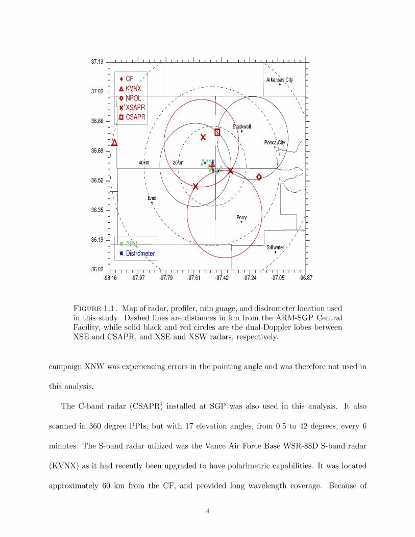
instruments and cameras for analyzing the hydrometeor types in the clouds. The locations
of the ground instruments utilized in this research are shown in Fig.1.1.
This analysis focused on the network of scanning precipitation radars, while using other
instruments for comparisons and validation of the results. There were three X-band radars
(referred to by their location relative the the central facility, CF, eg. XSW for the X-band
radar located to the southwest of the CF). These radars were located approximately 20
to 25 km apart and are able to scan over a 40 km range. They scanned over a 6 minute
period consisting of 360 degree PPIs (plan position indicator) at 22 elevations, with the
lowest elevation being 0.5 degrees and the highest being 50 degrees. However, during this
3
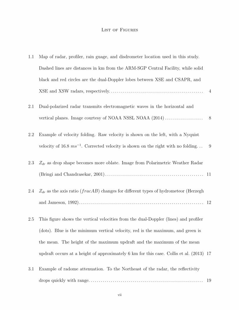
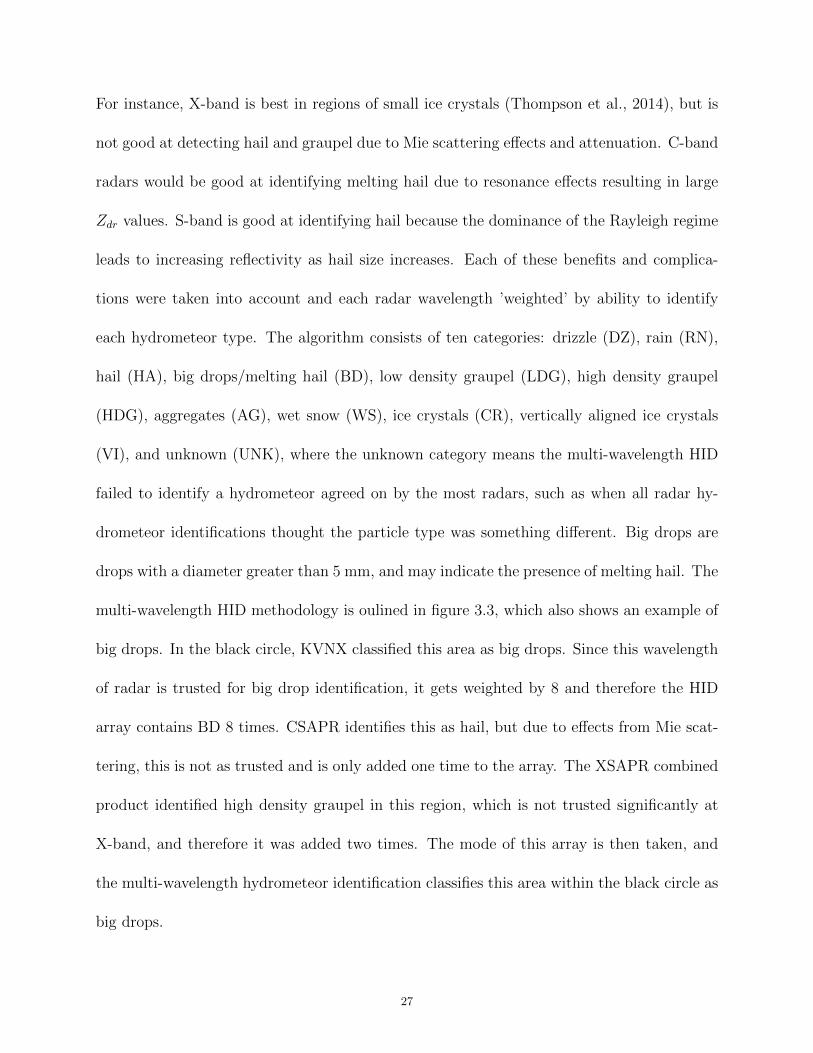
Figure 1.1. Map of radar, profiler, rain guage, and disdrometer location usedin this study. Dashed lines are distances in km from the ARM-SGP CentralFacility, while solid black and red circles are the dual-Doppler lobes betweenXSE and CSAPR, and XSE and XSW radars, respectively.
campaign XNW was experiencing errors in the pointing angle and was therefore not used in
this analysis.
The C-band radar (CSAPR) installed at SGP was also used in this analysis. It also
scanned in 360 degree PPIs, but with 17 elevation angles, from 0.5 to 42 degrees, every 6
minutes. The S-band radar utilized was the Vance Air Force Base WSR-88D S-band radar
(KVNX) as it had recently been upgraded to have polarimetric capabilities. It was located
approximately 60 km from the CF, and provided long wavelength coverage. Because of
4
the range to storms of interest, KVNX also routinely ”topped” storms of interest, which
the X-band radars were unable to do at times. Also present was the NASA S-Band Dual-
Polarization Radar (NPOL). This radar was not used in analysis, as it is a mobile radar and
not a permanent fixture at SGP. During MC3E it would also switch to range height indicator
(RHI) scans or sector scans for coordinated flights, which made it difficult to use for statistical
analysis. For this research, focus was placed on using ARM-DOE X- and C-band radars to
illustrate the use of the permanent instruments at SGP. An S-Band profiler located at the CF
was used to (in part) validate wind analysis. Soundings were launched from nearby Lamont,
Oklahoma (KLMN) every three hours during the MC3E field campaign, and continue to be
launched every 6 hours, providing good coverage of the atmospheric environment in which
the storms are forming. MC3E also deployed a sounding network, providing more soundings
than just at Lamont, Oklahoma. These soundings were merged into one product which was
used to auto-unfold velocities using a four-dimensional doppler dealiasing (4DD) algorithm
in PyArt, an open source python module for analysis of radar data (Heistermann et al.,
2014), by supplying information about the advection of the storms.
1.3. Organization
This research focuses on the case studies from the Northern Oklahoma region, both during
MC3E and from a winter event. The organization of this thesis is as follows. In chapter 2,
we will cover the previous work done utilizing dual-Doppler analysis as well as hydrometeor
identification algorithms. We will also discuss the model used for comparison to one case.
In chapter 3 we will discuss the methodology used in the analysis of the case studies. In
chapter 4, each case study will be discussed in detail individually, then the storm analysis
5
will be compared to get a better understanding of the differences in each case. Finally, we
will wrap up the research discussion with the findings and conclusions in chapter 5.
6
CHAPTER 2
Background
2.1. Dual-Polarized Radar
In this study, all radars used are dual-polarized, meaning they can transmit electromag-
netic waves in both the horizontal and vertical planes, as shown in Fig.2.1. In a basic sense,
polarized radars provide information on the shape, phase, and orientation of precipitation
particles, information that is not possible with a single polarization radar. Polarimetric
variables will be discussed later in this section. Dual-polarimetric radars may also pro-
vide improved rainfall estimates, as well as a better indication of hail versus heavy rain,
which would allow for more accurate flood or severe storm warnings with a larger lead time
(Rinehart, 2010). Hydrometeor classifications may also be determined through the available
variables, as was shown by Dolan and Rutledge (2009). Data are binned with range into so
called range bins, which depend on the pulse length transmitted by a radar. For a typical
one microsecond pulse, the range bin depth is 150 m.
The radar transmits electromagnetic waves into the atmosphere. When these waves
encounter a hydrometeor, the hydrometeor absorbs the energy, and reradiates the wave.
This return wave is then measured by the radar (Bringi and Chandrasekar, 2001). Often,
these targets are moving towards or away from the radar. This causes a frequency shift
between the EM waves transmitted from the radar and the EM waves reradiated back from
the particle to the radar, also called the Doppler shift (Rinehart, 2010). This is related to
the velocity of the particle. Velocity scans from a radar show the radial component of the
particle’s motion only. In order to get zonal, meridional, and vertical motions, multi-Doppler
7
Figure 2.1. Dual-polarized radar transmits electromagnetic waves in thehorizontal and vertical planes. Image courtesy of NOAA NSSL NOAA (2014)
analysis must be performed, which will be discussed in the following chapter. The maximum
Doppler velocity is called the Nyquist velocity, and may be calculated as:
Vmax =λPRF
4
where λ is the wavelength of the radar used, in meters. The PRF, or Pulse Repetition
Frequency, is the number of pulses emitted per second, and also affects the maximum range
of the radar as Rmax = c2PRF
, where c is the speed of light (Rinehart, 2010). Increasing
the PRF will increase the maximum velocity that may be sampled unambiguously, but
will decrease the maximum range invoking the possibility of second trip echoes. This is
known as the Doppler Dilemma (Rinehart, 2010)), which illustrates the struggle in finding a
8
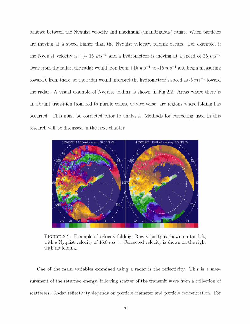
balance between the Nyquist velocity and maximum (unambiguous) range. When particles
are moving at a speed higher than the Nyquist velocity, folding occurs. For example, if
the Nyquist velocity is +/- 15 ms−1 and a hydrometeor is moving at a speed of 25 ms−1
away from the radar, the radar would loop from +15 ms−1 to -15 ms−1 and begin measuring
toward 0 from there, so the radar would interpret the hydrometeor’s speed as -5 ms−1 toward
the radar. A visual example of Nyquist folding is shown in Fig.2.2. Areas where there is
an abrupt transition from red to purple colors, or vice versa, are regions where folding has
occurred. This must be corrected prior to analysis. Methods for correcting used in this
research will be discussed in the next chapter.
Figure 2.2. Example of velocity folding. Raw velocity is shown on the left,with a Nyquist velocity of 16.8 ms−1. Corrected velocity is shown on the rightwith no folding.
One of the main variables examined using a radar is the reflectivity. This is a mea-
surement of the returned energy, following scatter of the transmit wave from a collection of
scatterers. Radar reflectivity depends on particle diameter and particle concentration. For
9
example, hail is very large so it would reflect a large amount of energy back to the radar and
return a high value of reflectivity. An area of heavy rainfall would contain many drops and
would also have a high reflectivity.
The reflectivity at the horizontal polarization (Zh) may be calculated as follows (Bringi
and Chandrasekar, 2001):
Zh =λ4
π5|Kp|2
∫D
|Shh(r,D)|2N(D)dD
where λ is the wavelength of the radar, Kp is the dielectric coefficient, Shh is the hor-
izontal element of the scattering matrix for both transmitted and backscattered waves, D
is the drop size diameter, r is the axis ratio of the hydrometeor, and N(D) is the drop size
distribution over the range bin sampled, but is often assumed to be the Marshall-Palmer
size distribution (Marshall and Palmer, 1948). Vertical bars denote the magnitude of the
element they surround. A similar calculation may be done to retrieve the vertically polarized
reflectivity. For Rayleigh backscatter, Shh increases as nearly D6, so that we may say (Bringi
and Chandrasekar, 2001)
|Shh|2≈ D6
This shows that reflectivity may be approximated to be a function of the sixth moment
of the drop size distribution (Bringi and Chandrasekar, 2001).
Differential reflectivity, or Zdr, is the ratio of the horizontal returned power to the vertical
returned power, and is a funciton of drop shape, phase (water vs. ice), and size (Bringi and
Chandrasekar, 2001). It may be calculated as:
10
Zdr =
∫|Shh(r,D)|2N(D)dD∫|Svv(r,D)|2N(D)dD
where Svv is the vertical element of the scattering matrix for both transmitted and
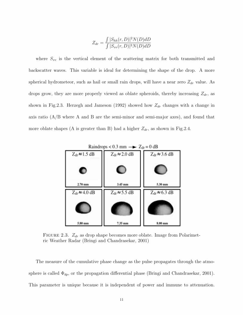
backscatter waves. This variable is ideal for determining the shape of the drop. A more
spherical hydrometeor, such as hail or small rain drops, will have a near zero Zdr value. As
drops grow, they are more properly viewed as oblate spheroids, thereby increasing Zdr, as
shown in Fig.2.3. Herzegh and Jameson (1992) showed how Zdr changes with a change in
axis ratio (A/B where A and B are the semi-minor and semi-major axes), and found that
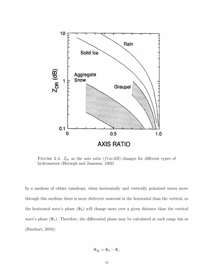
more oblate shapes (A is greater than B) had a higher Zdr, as shown in Fig.2.4.
Figure 2.3. Zdr as drop shape becomes more oblate. Image from Polarimet-ric Weather Radar (Bringi and Chandrasekar, 2001)
The measure of the cumulative phase change as the pulse propagates through the atmo-
sphere is called Φdp, or the propagation differential phase (Bringi and Chandrasekar, 2001).
This parameter is unique because it is independent of power and immune to attenuation.
11
Figure 2.4. Zdr as the axis ratio (fracAB) changes for different types ofhydrometeor (Herzegh and Jameson, 1992)
In a medium of oblate raindrops, when horizontally and vertically polarized waves move
through this medium there is more dielectric material in the horizontal than the vertical, so
the horizontal wave’s phase (Φh) will change more over a given distance than the vertical
wave’s phase (Φv). Therefore, the differential phase may be calculated at each range bin as
(Rinehart, 2010):
Φdp = Φh − Φv
12
The phase change will be larger in areas of heavy precipitation, and also depends heavily
on the path length of the pulse. In non-Rayleigh scattering regimes, phase fluctuations may
be caused by the phase shift from backscattered EM waves (δ), which can be found from the
difference between the total phase and the propagation differential phase.
Kdp, or specific differential phase, is the range derivative of Φdp. It may be calculated
from Hubbert and Bringi (1995) in terms of degrees of phase shift per kilometer along the
radial as:
Kdp =Φdp(r2)− Φdp(r1)
2(r2 − r1)
where r is the range in km along the radial, while the 2 in the denominator accounts for
the trip out to the range interval in question and back to the radar by the pulse. A target
with a near zero Kdp will be randomly oriented or almost spherical in shape. A positive value
indicates that the target is larger in the horizontal than in the vertical, such as raindrops,
while a negative value means the targets are larger in the vertical than the horizontal, such
as some forms of graupel and vertically aligned ice (Rinehart, 2010).
The co-polar correlation coefficient, or ρhv, is the correlation between the horizontally
and vertically polarized pulses at the same location and time (Rinehart, 2010) and may be
calculated as:
|ρhv|=〈nSvvShh〉
(〈n|Shh|2〉〈n|Svv|2〉)12
as shown by Bringi and Chandrasekar (2001; Eq. 7.41a). This variable can provide
information about the shape of drops, degree of melting, and the mixture of particles within
13
a volume. Rain would have a value of approximately 1, whereas hail, snow, graupel, and
ice crystals would have smaller values (slightly less than one) due to their irregular shapes,
random orientations, and mixes of water and ice. ρhv can also affected by noise, which
causes a decrease in the correlation, meaning that as the signal-to-noise ratio gets small, ρhv
decreases. For mixtures of ice and water, values of ρhv can be considerably smaller than 0.9.
By utilizing each of the polarimetric radar variables, a hydrometeor classification algo-
rithm may be created, as was done by many studies, such as Liu and Chandrasekar (2000),
Baldini et al. (2005), Dolan and Rutledge (2009) (henceforth D09), and Dolan et al. (2013)
(henceforth D13). D09 and D13 used simulations from a T-matrix scattering model of differ-
ent types of hydrometeors to create one-dimensional fuzzy logic membership beta functions,
which can then be applied to radar data to arrive at a hydrometeor classification for a given
range bin or grid block. The hydrometeor classification scheme used in this research was
based on D09 and D13, and will be discussed in more detail in the following chapter.
2.2. Multi-Doppler Analysis Previous Work
There have been a multitude of previous studies using dual- or multi-Doppler methods
in various applications as well as integrating these winds with a hydrometeor classification
to examine the inner workings of the clouds and storms.
One study by Ray et al. (1980) used single and multi-Doppler radar observations to
examine a tornadic storm on 20 May 1977 in central Oklahoma. Previously, focus had been
on single-Doppler methods to determine three dimensional storm motions through implied
areas of convergence and divergence. This study compared the different methods and found
that with more information (i.e. more radars available), the wind analysis had a smaller
14
error, but found that there was little difference between the two radar analysis and the four
radar analysis in terms of estimated error. They also found that there should be no more
than a few minutes between scans in order to minimize storm motion or evolution effects,
and that the radar scans in convective cases should include elevation angles greater than 30
degrees so that particle fall speed may be approximately estimated (Ray et al., 1980).
On 19 May 1977, a squall line formed in Oklahoma. Kessinger et al. (1987) studied the
convective and stratiform structure of this system using multiple Doppler analysis using the
NSSL 1977 Spring Program radars (S-bands Norman, Cimaron, and CHILL, and C-band
NCAR CP-4). Kessinger found that in general, flow parallel to the squall line was stronger
than the perpendicular flow. Kessinger et al. (1987) also found that the updrafts tilted
toward the west at low levels and toward the east at upper levels in the mature convective
region.
In 1991, a study was completed on a squall line in Southern Germany by Meischner et
al.(1991). This study used single-Doppler analysis to arrive at zonal and meridional flow
patterns as well as determining hail sizes and distinguishing regions of rain from regions
of rain-hail mixtures. Their findings revealed that so-called big drops existed in the feeder
clouds of the squall line and played an important role in the hail formation process (Meischner
et al., 1991).
More recently, a study was done by Dolan and Rutledge (2010) that used the CASA IP1
network of four X-band radars in central Oklahoma to examine kinematic and microphys-
ical interactions in the 10 June 2007 convective storms. They used the D09 hydrometeor
classification algorithm to arrive at the microphysical composition of the storms, and the
15
NCAR-CEDRIC package to perform multi-Doppler analysis to arrive at the kinematics. It
was found that the updraft development lead to graupel formation, which was followed by
intra-cloud lightning, with cloud to ground lightning beginning once high density graupel
was found at mid-levels. As more graupel was suspended in the updraft, a downdraft begins
forming, bringing precipitation to the surface, causing CG flashes to decrease.
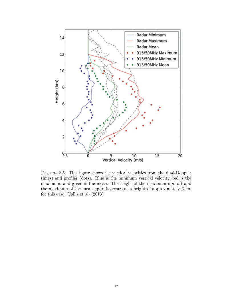
Collis et al. (2013) examined the statitistics of storm updraft velocities in Darwin, Aus-
tralia during the Tropical Warm Pool International Cloud Experiment (TWP-ICE) using
dual-Doppler analysis, which was also compared to the vertical velocities observed by a
nearby profiler. They found that the profiler is unable to fully capture the three dimensional
storm structure as it is a point-time measurement.
In examining the vertical velocity profile, they found the mean height of the maximum
updraft to occur at approximately 6 to 8 km above ground, as shown in Fig.2.5, which is
lower than was found in a previous modeling study by Wu et al. (2009), who found this
occured at a height of 12 km in the WRF model they ran.
A study by Fujiyoshi et al. (1998) examined longitudinal snowbands containing convective
cloud systems near Ishikari Bay, Hokkaido Japan on 15 January 1992 using two X-band radars
to provide dual-Doppler kinematics. In general, they studied the horizontal wind component
as their snow bands did not have strong vertical motions. They did find, however, that the
updrafts were found to the front of the systems, and were responsible for transporting ice
and snow toward the rear of the bands, where it evaporated outside the clouds causing a
downdraft.
16
Figure 2.5. This figure shows the vertical velocities from the dual-Doppler(lines) and profiler (dots). Blue is the minimum vertical velocity, red is themaximum, and green is the mean. The height of the maximum updraft andthe maximum of the mean updraft occurs at a height of approximately 6 kmfor this case. Collis et al. (2013)
17
CHAPTER 3
Methodology
This section discusses what was done to quality control the radar data, such as correcting
for biases and attenuation. We also present the methodology for analyzing the data.
3.1. Quality Control
The first step in analyzing data is to ensure the data set is of high quality. For many of the
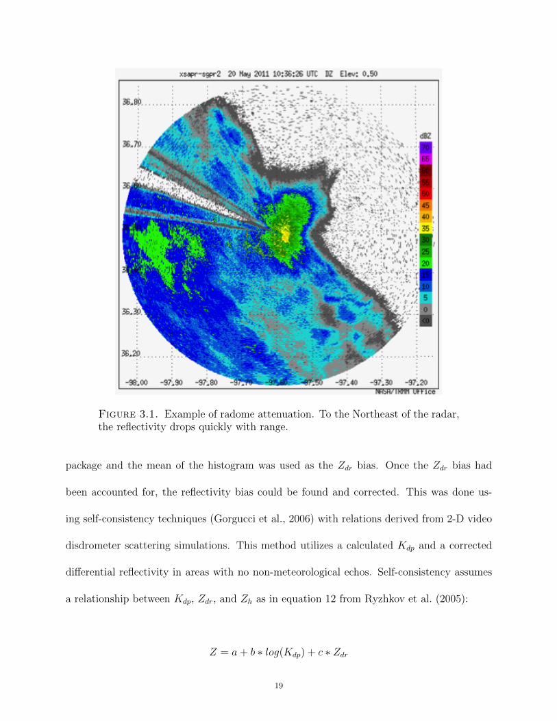
cases analyzed during MC3E, the storms rained heavily on the radomes of the CSAPR and
the two XSAPRS, causing a significant drop in reflectivity with range, such as that shown in
figure 3.1; this is termed radome attenuation. This made these times unusable for kinematic
and microphysical analysis. If the scans suffering from this were only a small portion of
the ideal time period, they were removed from analysis. If the radar was contaminated by
radome attenuation for a longer portion of the ideal time frame, the analysis time period
was cut short. This was done for the 20 May 2011 case, as a strong squall line moved over
the radars and we were unable to get data from the strongest portion of the storm or during
the period of the trailing stratiform region.
All four of the radars used suffered from reflectivity and differential reflectivity biases.
The differential reflectivity biases were calculated using vertically pointing scans when avail-
able, horizon-to-horizon RHI scans (Ryzhkov et al., 2005)), or from a high elevation angle
scan through stratiform rain when neither of the other types of scans listed were available.
In these chosen scan types and regions of precipitation, it is assumed that the radars should
see a Zdr of 0 dB. Histograms were created in these regions using the NCAR SOLOii editting
18
Figure 3.1. Example of radome attenuation. To the Northeast of the radar,the reflectivity drops quickly with range.
package and the mean of the histogram was used as the Zdr bias. Once the Zdr bias had
been accounted for, the reflectivity bias could be found and corrected. This was done us-
ing self-consistency techniques (Gorgucci et al., 2006) with relations derived from 2-D video
disdrometer scattering simulations. This method utilizes a calculated Kdp and a corrected
differential reflectivity in areas with no non-meteorological echos. Self-consistency assumes
a relationship between Kdp, Zdr, and Zh as in equation 12 from Ryzhkov et al. (2005):
Z = a+ b ∗ log(Kdp) + c ∗ Zdr
19
Here the coefficients a, b, and c are determined for each radar wavelength from 2DVD
scattering simulations. The reflectivity offset is then determined by incrementally adjusting
Z from Zmin to Zmax to match the following integrals (equations 14 and 15 from Ryzhkov
et al. (2005)):
I1 =
∫ Zmax
Zmin
〈Kdp(Z)〉n(Z)dz
I2 =
∫ Zmax
Zmin
10−ab+Z
b− c〈Zdr(Z)〉
b n(Z)dz
where n(Z) is defined as the number of data pixels, or gates, for a given 1 dB interval
of reflectivity between the limits of the integral. When the integrals match, this Zh is the
correct value, and the difference between this and the original is the offset.
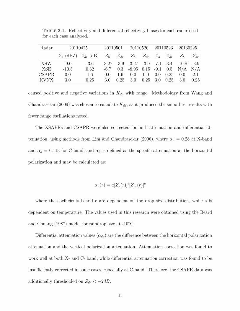
The Z and Zdr biases are listed in Table 3.1. The Southwest XSAPR (XSW) had the
largest Zdr bias, of approximately -3.6 dB for most of the cases. Overall we found KVNX
to have consistent biases over each case in both reflectivity and Zdr, while CSAPR was
consistent for reflectivity only and varied for Zdr for upwards of 1 dB for each case. The
XSAPRs varied widely in reflectivity biases but were relatively consistent for differential
reflectivity biases. After these corrections, the data is assumed to be calibrated to within
0.2 dB for Zdr and 1 dB for reflectivity.
Another problem was a large decreasing trend in differential phase over a short range.
This caused issues when calculating specific differential phase (Kdp). During calculations,
delta effects due to Mie scattering, meaning that the backscatter differential phase gets noisy
in Mie scattering regimes, making it difficult to remove from Φdp calculations and therefore
20
Table 3.1. Reflectivity and differential reflectivity biases for each radar usedfor each case analyzed.
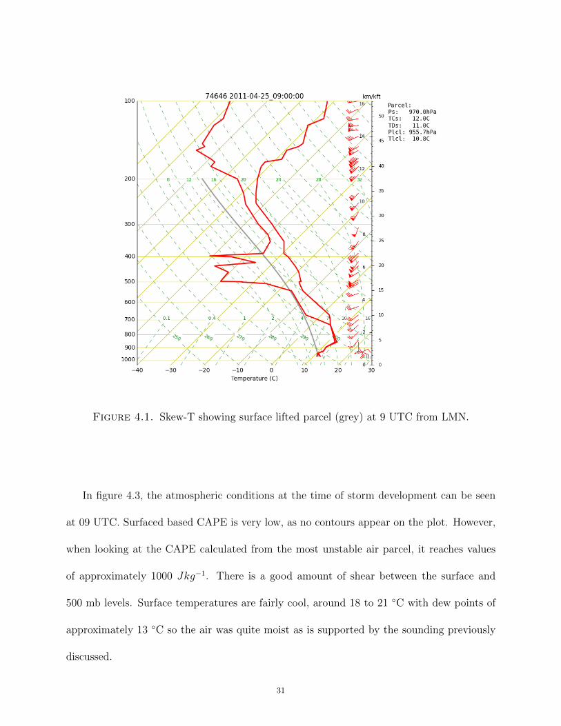
Figure 4.1. Skew-T showing surface lifted parcel (grey) at 9 UTC from LMN.
In figure 4.3, the atmospheric conditions at the time of storm development can be seen
at 09 UTC. Surfaced based CAPE is very low, as no contours appear on the plot. However,
when looking at the CAPE calculated from the most unstable air parcel, it reaches values
of approximately 1000 Jkg−1. There is a good amount of shear between the surface and
500 mb levels. Surface temperatures are fairly cool, around 18 to 21 ◦C with dew points of
approximately 13 ◦C so the air was quite moist as is supported by the sounding previously
discussed.
31
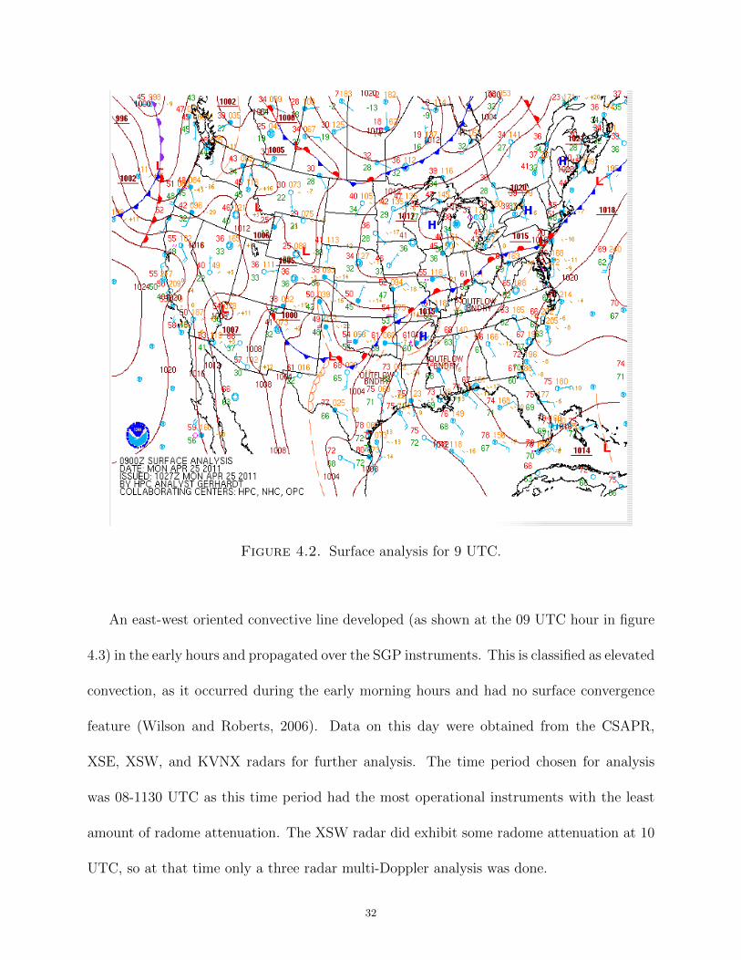
Figure 4.2. Surface analysis for 9 UTC.
An east-west oriented convective line developed (as shown at the 09 UTC hour in figure
4.3) in the early hours and propagated over the SGP instruments. This is classified as elevated
convection, as it occurred during the early morning hours and had no surface convergence
feature (Wilson and Roberts, 2006). Data on this day were obtained from the CSAPR,
XSE, XSW, and KVNX radars for further analysis. The time period chosen for analysis
was 08-1130 UTC as this time period had the most operational instruments with the least
amount of radome attenuation. The XSW radar did exhibit some radome attenuation at 10
UTC, so at that time only a three radar multi-Doppler analysis was done.
32
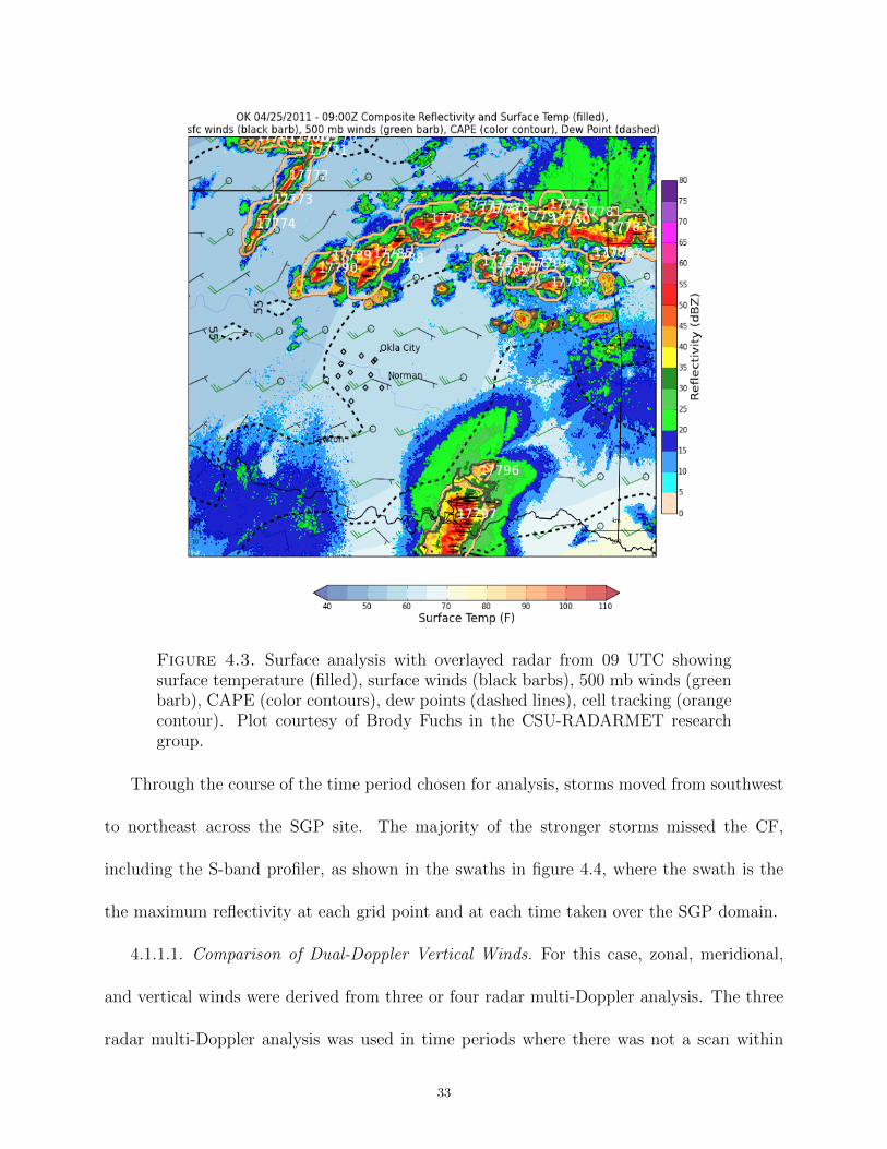
Figure 4.3. Surface analysis with overlayed radar from 09 UTC showingsurface temperature (filled), surface winds (black barbs), 500 mb winds (greenbarb), CAPE (color contours), dew points (dashed lines), cell tracking (orangecontour). Plot courtesy of Brody Fuchs in the CSU-RADARMET researchgroup.
Through the course of the time period chosen for analysis, storms moved from southwest
to northeast across the SGP site. The majority of the stronger storms missed the CF,
including the S-band profiler, as shown in the swaths in figure 4.4, where the swath is the
the maximum reflectivity at each grid point and at each time taken over the SGP domain.
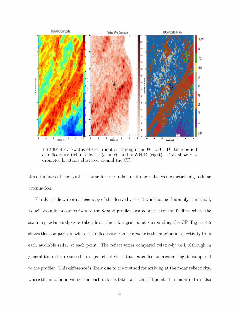
4.1.1.1. Comparison of Dual-Doppler Vertical Winds. For this case, zonal, meridional,
and vertical winds were derived from three or four radar multi-Doppler analysis. The three
radar multi-Doppler analysis was used in time periods where there was not a scan within
33
Figure 4.4. Swaths of storm motion through the 08-1130 UTC time periodof reflectivity (left), velocity (center), and MWHID (right). Dots show dis-drometer locations clustered around the CF.
three minutes of the synthesis time for one radar, or if one radar was experiencing radome
attenuation.
Firstly, to show relative accuracy of the derived vertical winds using this analysis method,
we will examine a comparison to the S-band profiler located at the central facility, where the
scanning radar analysis is taken from the 1 km grid point surrounding the CF. Figure 4.5
shows this comparison, where the reflectivity from the radar is the maximum reflectivity from
each available radar at each point. The reflectivities compared relatively well, although in
general the radar recorded stronger reflectivities that extended to greater heights compared
to the profiler. This difference is likely due to the method for arriving at the radar reflectivity,
where the maximum value from each radar is taken at each grid point. The radar data is also
34
for the 1 km box surrounding the profiler, and therefore may include stronger reflectivities.
Vertical velocity values also compared well, particularly in the convective updraft regions
(red shades), in terms of both strength and location, while downdraft regions were disagreed
in terms of both strength and location, with the profiler showing more downdraft regions
than the radar.
Figure 4.5. Comparison of interpolated profiler and composite radar reflec-tivity (a, c) and vertical winds (b,d) for 25 April 2011.
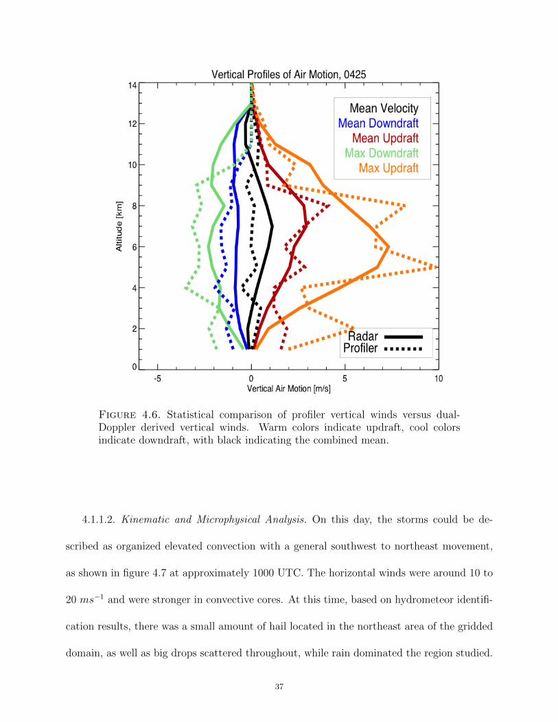
When examining statistics in more detail, as shown in figure 4.6, the magnitudes of the
updrafts generally agreed to within the expected error value of 1 ms−1. Both the profiler
and the radar derived vertical winds saw the mean values peak at approximately 8 km in
35
height. The maximum updraft has more variation in the higher resolution profiler data than
the radar derived winds, but both have a similar shape and have peaks at approximately
5.5 km in height. In contrast, the downdraft regions have the largest differences. Below
approximately 10 km, the profiler measures vertical wind speeds that are consistently larger
than those found by the multi-Doppler analysis for both mean and maximum downdraft
velocities. In general the difference is still on the order of 1 ms−1 in most areas. These larger
downdraft values contribute to the overall mean velocity by making it more consistent at 0
ms−1, while the multi-Doppler vertical wind speed means exhibit upward motion dominating
in the mid to upper levels of the atmosphere and downward motions dominating the lower
regions of the storm and the extreme upper regions.
The differences between the profiler and dual-Doppler winds noted above may be attrib-
uted to a number of things. First, the profiler data was smoothed to match the resolution of
the radar data in both time and space, while the multi-Doppler winds were shown only for
the column directly above the profiler. The large varying areas of updraft are likely caused
by the high resolution of the profiler data, resulting in higher values. Another reason for the
differences could be due to the difficulty of the scanning radars to detect surface divergence
due to beam geometry (Nelson and Brown, 1987). There may also be errors in the fall speed
being applied to the profiler.
Based on this comparison, we conclude that the multi-Doppler wind analysis is able to
recover vertical motions to within 1 ms−1 with a bias for underestimating downward motions
and may therefore be used in this and other cases to examine the three dimensional kinematic
structure of convective storms.
36
Figure 4.6. Statistical comparison of profiler vertical winds versus dual-Doppler derived vertical winds. Warm colors indicate updraft, cool colorsindicate downdraft, with black indicating the combined mean.
4.1.1.2. Kinematic and Microphysical Analysis. On this day, the storms could be de-
scribed as organized elevated convection with a general southwest to northeast movement,
as shown in figure 4.7 at approximately 1000 UTC. The horizontal winds were around 10 to
20 ms−1 and were stronger in convective cores. At this time, based on hydrometeor identifi-
cation results, there was a small amount of hail located in the northeast area of the gridded
domain, as well as big drops scattered throughout, while rain dominated the region studied.
37
Figure 4.7. Gridded image of reflectivity at 2 km with overlayed winds (left)and of hydrometeor classification (right) at 1001 UTC on 25 April 2011
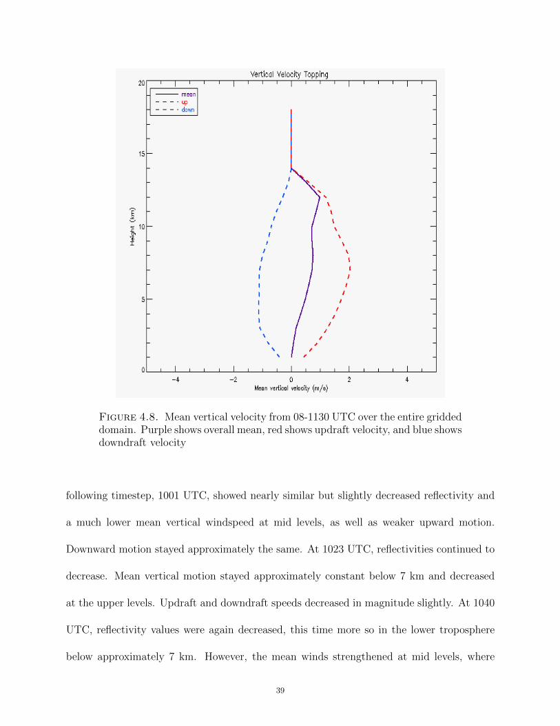
Total mean wind over the analysis domain and storm time frame of 0800 to 1130 UTC
are shown in figure 4.8. The total mean vertical wind speed is generally slightly upward over
the entire height of the storms. Mean downward motion has a maximum of -1.2 ms−1 and
occurs of heights ranging from 4 km to 7 km, while the updraft has a maximum mean of 2.5
ms−1 occurring at 7 km in height. Mean echo top is also shown to be approximately 14 km.
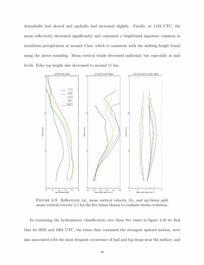
In order to examine the evolution of storms during this case, five times were selected over
the course of the analysis period, shown in figure 4.9. These times are: 0933 UTC, 1001
UTC, 1023 UTC, 1040 UTC, and 1123 UTC. The strongest reflectivities occurred during the
first two times (0933 and 1001 UTC). At 0933 UTC, the strong reflectivities corresponded
to stronger winds in both mean vertical motion and updraft and downdraft motion. The
38
Figure 4.8. Mean vertical velocity from 08-1130 UTC over the entire griddeddomain. Purple shows overall mean, red shows updraft velocity, and blue showsdowndraft velocity
following timestep, 1001 UTC, showed nearly similar but slightly decreased reflectivity and
a much lower mean vertical windspeed at mid levels, as well as weaker upward motion.
Downward motion stayed approximately the same. At 1023 UTC, reflectivities continued to
decrease. Mean vertical motion stayed approximately constant below 7 km and decreased
at the upper levels. Updraft and downdraft speeds decreased in magnitude slightly. At 1040
UTC, reflectivity values were again decreased, this time more so in the lower troposphere
below approximately 7 km. However, the mean winds strengthened at mid levels, where
39
downdrafts had slowed and updrafts had increased slightly. Finally, at 1123 UTC, the
mean reflectivity decreased significantly and contained a brightband signature common in
stratiform precipitation at around 4 km, which is consistent with the melting height found
using the above sounding. Mean vertical winds decreased uniformly but especially at mid
levels. Echo top height also decreased to around 11 km.
Figure 4.9. Reflectivity (a), mean vertical velocity (b), and up/down splitmean vertical velocity (c) for the five times chosen to evaluate storm evolution.
In examining the hydrometeor classification over these five times in figure 4.10 we find
that for 0933 and 1001 UTC, the times that contained the strongest upward motion, were
also associated with the most frequent occurrence of hail and big drops near the surface, and
40
high density graupel (HDG) in the midlevels. As the vertical velocities decreased, more low
density graupel (LDG) was found. This occurs because the lower vertical motions are unable
to support the larger and heavier ice particles, plus supercooled water contents available for
riming are also reduced. At the earlier (stronger) time periods, the height of the peak hail,
LDG, and HDG was high, and lowered as storms grew weaker. In the wet snow category,
there was a peak at the height of the melting layer, around 4 km. This was at its largest
frequency for 1123 UTC, when the echo pattern was highly stratiform in nature. This time
was also dominated by drizzle hydrometeors instead of rain and had the highest occurrence
of ice crystals and aggregates above the melting layer. Throughout each time, except the
final time, there is a large amount of hail shown at mid levels, but it does not appear to reach
the surface with the same frequency. Instead, big drops are found at the surface, moreso
during the stronger times (0933 and 1001 UTC). The Storm Prediction Center showed no
severe hail reports in the region of study. Therefore, it is likely that in this case the big
drops were likely formed through melting hail and graupel rather than collision-coalescence,
as the warm cloud depth was deep, giving the hail ample time to melt.
4.1.1.3. Model Comparison. This case provides a unique opportunity to statistically com-
pare the radar observations to the simulated storm output from the WRF-SBM model. In
order to do this, a convective-stratiform partitioning based on the method presented in
Steiner et al. (1995) was applied to both the radar observations and the model simulated
reflectivity. Reflectivity was then partitioned into shallow or deep categories, where shallow
was any column with an echo top height less than 6 km. The model simulated reflectivity
41
Figure 4.10. Frequency of each hydrometeor category as a function of heightfor each of the five chosen times for the 25 April case.
over a 100 km by 100 km area centered on the SGP central facility, which matches the mi-
crophysical retrieval domain for radar observations but is larger than the kinematic retrieval
domain of 60 x 60 km. Both radar and model have a 1 km vertical grid spacing. The model
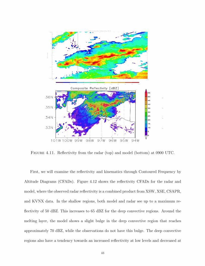
did relatively well with its analysis of the storm, as shown in Fig. 4.11, where storms are of
similar shape and organization. However, the model analyzes a much larger region, and saw
these storms further to the south of the SGP site, so direct comparison could not be done.
Statistical comparison of storm domain was instead utilized to compare the kinematic and
microphysical properties of the case.
42
Figure 4.11. Reflectivity from the radar (top) and model (bottom) at 0900 UTC.
First, we will examine the reflectivity and kinematics through Contoured Frequency by
Altitude Diagrams (CFADs). Figure 4.12 shows the reflectivity CFADs for the radar and
model, where the observed radar reflectivity is a combined product from XSW, XSE, CSAPR,
and KVNX data. In the shallow regions, both model and radar see up to a maximum re-
flectivity of 50 dBZ. This increases to 65 dBZ for the deep convective regions. Around the
melting layer, the model shows a slight bulge in the deep convective region that reaches
approximately 70 dBZ, while the observations do not have this bulge. The deep convective
regions also have a tendency towards an increased reflectivity at low levels and decreased at
43
the upper levels, whereas the model simulated reflectivity has a slight curve to lower reflec-
tivities near the surface. It appears the model simulations therefore have a more stratiform
like brightband signature at the melting layer even in regions of deep convection. This may
have occurred due to the way the model simulates reflectivity as a column, similar to a
profiler observation, which would enhance any melting layer signatures. Another possible
reason is that the Steiner et al. (1995) method has a tendency to include some deep strati-
form columns in the deep convective category due to the reflectivity biases intrinsic in the
WRF-SBM model. A sensitivity study was conducted by T. Matsui on this model using
different convective-stratiform classification methods, and found that a method based on
updraft velocity was the most accurate for the model, though this was not true for the radar
analysis.
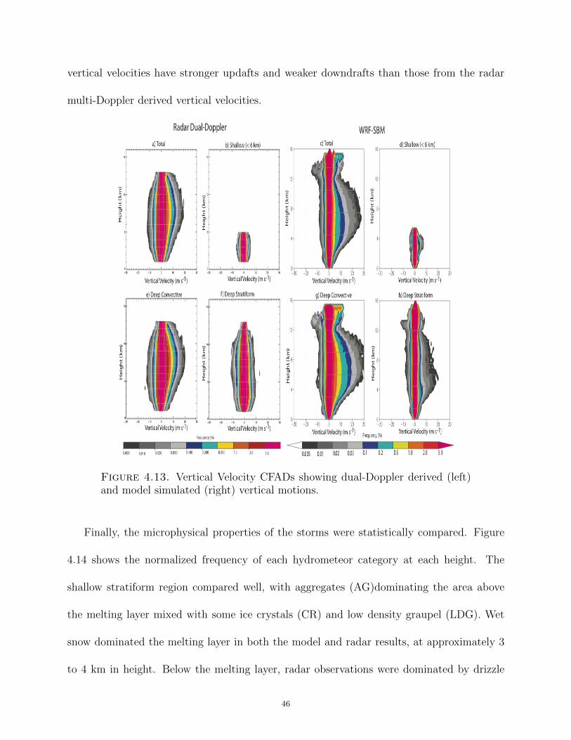
Next, vertical velocity CFADs were analyzed (Figure 4.13). At a quick glance, it can
be seen that the observed and simulated vertical velocities are in relative agreement as they
have similar shapes. However, differences in the maximum and minimum values are present.
Both model and radar observations agree that there is a peak in updraft speed around 7.5
km, but disagree in the magnitude of this peak. The radar shows it to be near 20 ms−1,
while the model shows it as 30 ms−1. These are both associated with the deep convective
regions of the storms. The radar observations also show midlevel downdrafts of slightly
larger values near -12 ms−1, whereas the model does not show any downdraft larger than
-10 ms−1. Another difference between the model and radar vertical velocities is cloud top
height. The radar observations are limited to 13 km in height, while the model sees increasing
velocities at higher levels, with a peak height of 16 km. The shallow CFADs compare well,
44
Figure 4.12. Reflectivity CFADs showing radar observations (left) andWRF-SBM simulations (right) for the 25 April 2011 case.
with all magnitudes less than |8| ms−1, although the model sees a small peak at the height
of the melting layer height. The deep stratiform region is the most different in both shape
and magnitude. The model sees larger updraft speeds, peaking to 20 ms−1 at a height of
5 km, while the radar observations only reach 10 ms−1 and do not have a clear maximum
peak height. These maximum values are too high for typical stratiform precipitation, but
these only occur in less than 0.1 % of the time. This is likely due to a possible convective
stratiform partition misclassification, especially in the model. Overall, the model simulated
45
vertical velocities have stronger updafts and weaker downdrafts than those from the radar
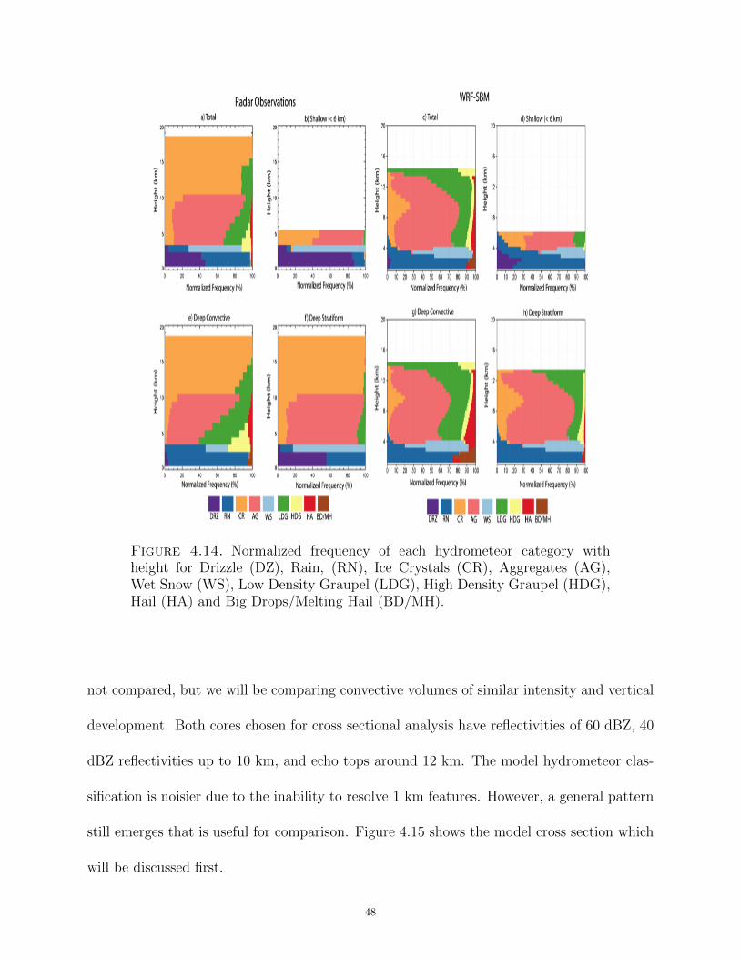
Finally, the microphysical properties of the storms were statistically compared. Figure
4.14 shows the normalized frequency of each hydrometeor category at each height. The
shallow stratiform region compared well, with aggregates (AG)dominating the area above
the melting layer mixed with some ice crystals (CR) and low density graupel (LDG). Wet
snow dominated the melting layer in both the model and radar results, at approximately 3
to 4 km in height. Below the melting layer, radar observations were dominated by drizzle
46
(DZ, >80%) while rain (RN, 80%) dominated in the model simulations. The model also
showed rain above the melting layer, associated with supercooled liquid water droplets aloft
that the radar observations did not identify. Between the model and the radar observations,
the deep stratiform region was similar below 10 km, although the model also noted the
presense of high density graupel (HDG) aloft and saw hail (HA) and big drops (BD) at the
surface. The radar observations again saw drizzle dominating below the melting layer, while
the model was dominated by rain and also saw some supercooled liquid water drops above
the melting layer. Above 10 km, the radar observations showed the clouds to consist mostly
of ice crystals, while the model saw appreciable amounts of ice crystals, aggregates, and low
density graupel, mixed with a small amount of high density graupel. In the deep convective
regions, the agreement between radar and model was similar again below 10 km. The model
shows a higher frequency hail and big drops at low levels, with some hail even reaching the
surface, whereas the observations see hail aloft and only big drops at the surface, both in
lower frequencies than the simulations. The presense of hail at the surface noted in the model
was not observed in the region, as there were no hail reports associated with storms on this
day. Above 10 km, once again, drastic differences were found between the MWHID run on
the radar analysis and the microphysical classifications of the model simulations. The radar
observations show a majority of ice crystals with a mix of low density graupel, while the
model shows a mix of all the ice hydrometeor categories, except wet snow, in large fractions.
In order to better understand the differences noted in the statistical comparisons be-
tween the hydrometeor classifications for the radar and model simulation, we must look at
a vertical cross section from both. Due to location and timing differences, exact cores are
47
Figure 4.14. Normalized frequency of each hydrometeor category withheight for Drizzle (DZ), Rain, (RN), Ice Crystals (CR), Aggregates (AG),Wet Snow (WS), Low Density Graupel (LDG), High Density Graupel (HDG),Hail (HA) and Big Drops/Melting Hail (BD/MH).
not compared, but we will be comparing convective volumes of similar intensity and vertical
development. Both cores chosen for cross sectional analysis have reflectivities of 60 dBZ, 40
dBZ reflectivities up to 10 km, and echo tops around 12 km. The model hydrometeor clas-
sification is noisier due to the inability to resolve 1 km features. However, a general pattern
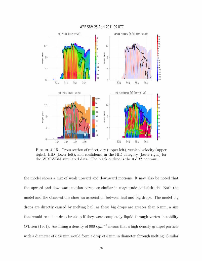
still emerges that is useful for comparison. Figure 4.15 shows the model cross section which
will be discussed first.
48
In figure 4.15, the black line represents the 0 dBZ threshold for reflectivity used for HID
model statistics in figure 4.14. In the HID profile, this means that the majority of ice crystals
aloft and drizzle below the melting layer were not shown in the statistical analysis. There
is also a region of low confidence (less than 40%) at the transition in classification between
aggregates and ice crystals, as well as around regions of big drops. Confidence is high in
the convective core above the melting layer and in the stratiform region, and is moderate
in other regions surrounding the convective core. The model also showed hail cores aloft
that were surrounded by low density graupel, and revealed aggregates in regions of weaker
echoes near storm edges and in the stratiform region on the downshear side of the storm.
Confidence is highest in the hail cores and decreases quickly in the surrounding region of low
density graupel. The low to moderate confidence surrounding the convective core suggests
that the model has a mix of many different hydrometeor types in these regions.
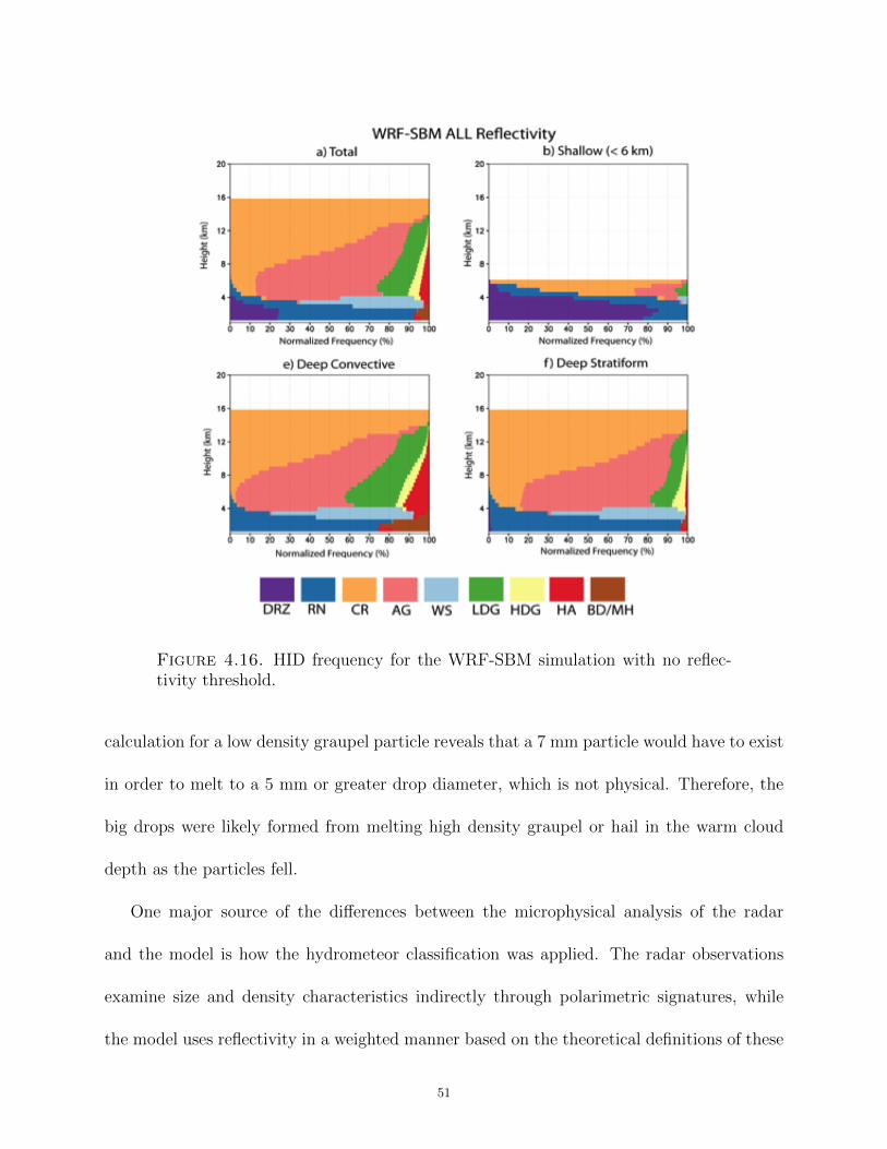
Without the 0 dBZ threshold, the statistical comparison has much better agreement, as
shown in figure 4.16 a, b, e, f compared with the observations in figure 4.14. Ice crystals
now dominate above 10 km in height, and below drizzle is now present in the shallow regime
below the melting layer. Therefore, it can be concluded that the model underestimated the
radar reflectivitity of ice crystals and drizzle.
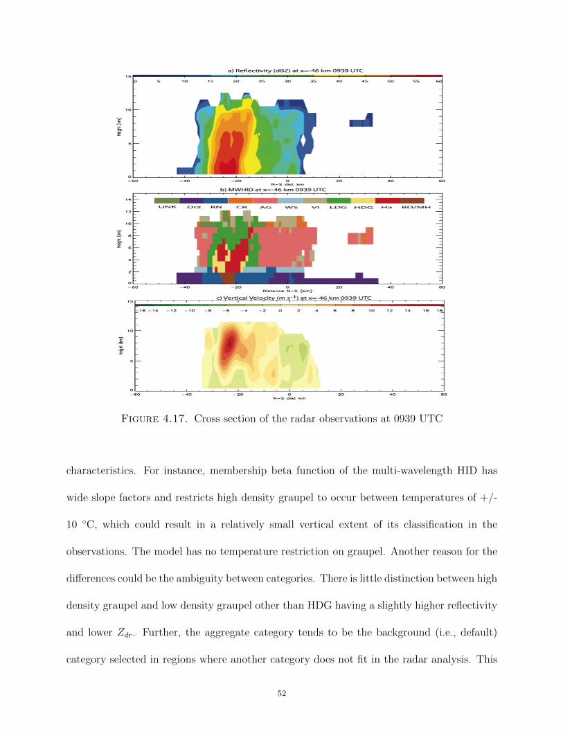
Comparing this cross-section to one from the radar observations (figure 4.17), we see
similar trends of hail aloft encircled by low density graupel, and big drops below the hail at
the surface. It is difficult to compare the vertical velocities, as the model cross section has
many small cores and the radar cross section has one main core. However, it can be noted
that in the stratiform region, the radar observations show more downward motion while
49
Figure 4.15. Cross section of reflectivity (upper left), vertical velocity (upperright), HID (lower left), and confidence in the HID category (lower right) forthe WRF-SBM simulated data. The black outline is the 0 dBZ contour.
the model shows a mix of weak upward and downward motions. It may also be noted that
the upward and downward motion cores are similar in magnitude and altitude. Both the
model and the observations show an association between hail and big drops. The model big
drops are directly caused by melting hail, as these big drops are greater than 5 mm, a size
that would result in drop breakup if they were completely liquid through vortex instability
O’Brien (1961). Assuming a density of 900 kgm−3 means that a high density graupel particle
with a diameter of 5.25 mm would form a drop of 5 mm in diameter through melting. Similar
50
Figure 4.16. HID frequency for the WRF-SBM simulation with no reflec-tivity threshold.
calculation for a low density graupel particle reveals that a 7 mm particle would have to exist
in order to melt to a 5 mm or greater drop diameter, which is not physical. Therefore, the
big drops were likely formed from melting high density graupel or hail in the warm cloud
depth as the particles fell.
One major source of the differences between the microphysical analysis of the radar
and the model is how the hydrometeor classification was applied. The radar observations
examine size and density characteristics indirectly through polarimetric signatures, while
the model uses reflectivity in a weighted manner based on the theoretical definitions of these
51
Figure 4.17. Cross section of the radar observations at 0939 UTC
characteristics. For instance, membership beta function of the multi-wavelength HID has
wide slope factors and restricts high density graupel to occur between temperatures of +/-
10 ◦C, which could result in a relatively small vertical extent of its classification in the
observations. The model has no temperature restriction on graupel. Another reason for the
differences could be the ambiguity between categories. There is little distinction between high
density graupel and low density graupel other than HDG having a slightly higher reflectivity
and lower Zdr. Further, the aggregate category tends to be the background (i.e., default)
category selected in regions where another category does not fit in the radar analysis. This
52
implies that in the radar analysis, regions of aggregates may be close to another category,
one that the model simulation may have classified in the region. Had that category been
classified instead of aggregates, the comparison between model and observations may have
more similarities.
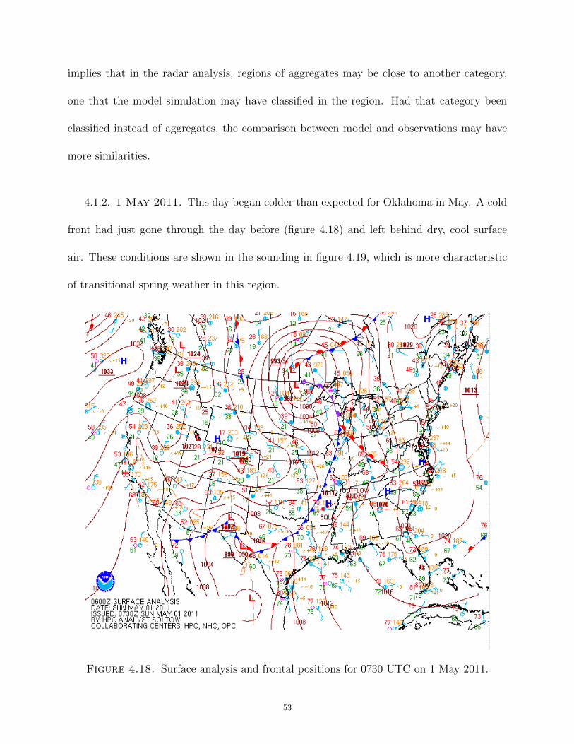
4.1.2. 1 May 2011. This day began colder than expected for Oklahoma in May. A cold
front had just gone through the day before (figure 4.18) and left behind dry, cool surface
air. These conditions are shown in the sounding in figure 4.19, which is more characteristic
of transitional spring weather in this region.
Figure 4.18. Surface analysis and frontal positions for 0730 UTC on 1 May 2011.
53
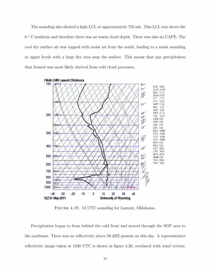
The sounding also showed a high LCL at approximately 750 mb. This LCL was above the
0 ◦ C isotherm and therefore there was no warm cloud depth. There was also no CAPE. The
cool dry surface air was topped with moist air from the south, leading to a moist sounding
at upper levels with a large dry area near the surface. This meant that any precipitaiton
that formed was most likely derived from cold cloud processes.
Figure 4.19. 12 UTC sounding for Lamont, Oklahoma.
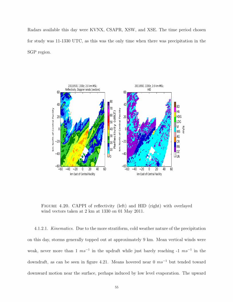
Precipitation began to form behind the cold front and moved through the SGP area to
the southeast. There was no reflectivity above 50 dBZ present on this day. A representative
reflectivity image taken at 1330 UTC is shown in figure 4.20, overlayed with wind vectors.
54
Radars available this day were KVNX, CSAPR, XSW, and XSE. The time period chosen
for study was 11-1330 UTC, as this was the only time when there was precipitation in the
SGP region.
Figure 4.20. CAPPI of reflectivity (left) and HID (right) with overlayedwind vectors taken at 2 km at 1330 on 01 May 2011.
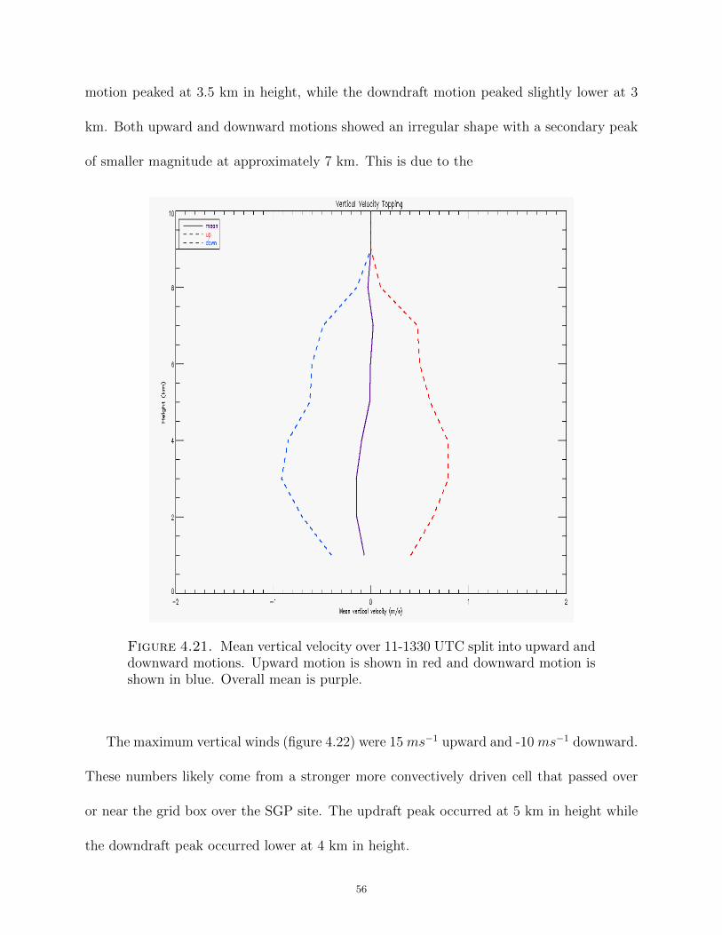
4.1.2.1. Kinematics. Due to the more stratiform, cold weather nature of the precipitation
on this day, storms generally topped out at approximately 9 km. Mean vertical winds were
weak, never more than 1 ms−1 in the updraft while just barely reaching -1 ms−1 in the
downdraft, as can be seen in figure 4.21. Means hovered near 0 ms−1 but tended toward
downward motion near the surface, perhaps induced by low level evaporation. The upward
55
motion peaked at 3.5 km in height, while the downdraft motion peaked slightly lower at 3
km. Both upward and downward motions showed an irregular shape with a secondary peak
of smaller magnitude at approximately 7 km. This is due to the
Figure 4.21. Mean vertical velocity over 11-1330 UTC split into upward anddownward motions. Upward motion is shown in red and downward motion isshown in blue. Overall mean is purple.
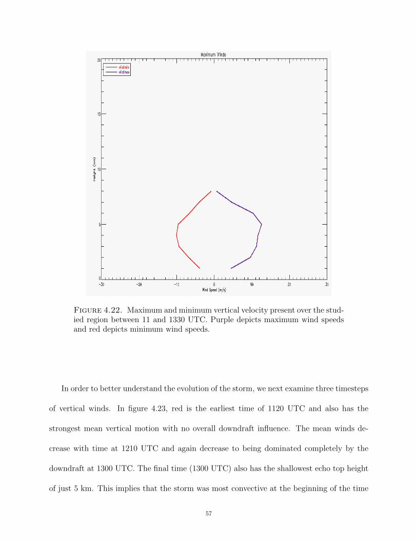
The maximum vertical winds (figure 4.22) were 15 ms−1 upward and -10 ms−1 downward.
These numbers likely come from a stronger more convectively driven cell that passed over
or near the grid box over the SGP site. The updraft peak occurred at 5 km in height while
the downdraft peak occurred lower at 4 km in height.
56
Figure 4.22. Maximum and minimum vertical velocity present over the stud-ied region between 11 and 1330 UTC. Purple depicts maximum wind speedsand red depicts minimum wind speeds.
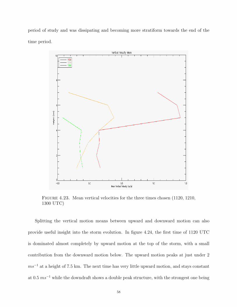
In order to better understand the evolution of the storm, we next examine three timesteps
of vertical winds. In figure 4.23, red is the earliest time of 1120 UTC and also has the
strongest mean vertical motion with no overall downdraft influence. The mean winds de-
crease with time at 1210 UTC and again decrease to being dominated completely by the
downdraft at 1300 UTC. The final time (1300 UTC) also has the shallowest echo top height
of just 5 km. This implies that the storm was most convective at the beginning of the time
57
period of study and was dissipating and becoming more stratiform towards the end of the
time period.
Figure 4.23. Mean vertical velocities for the three times chosen (1120, 1210,1300 UTC)
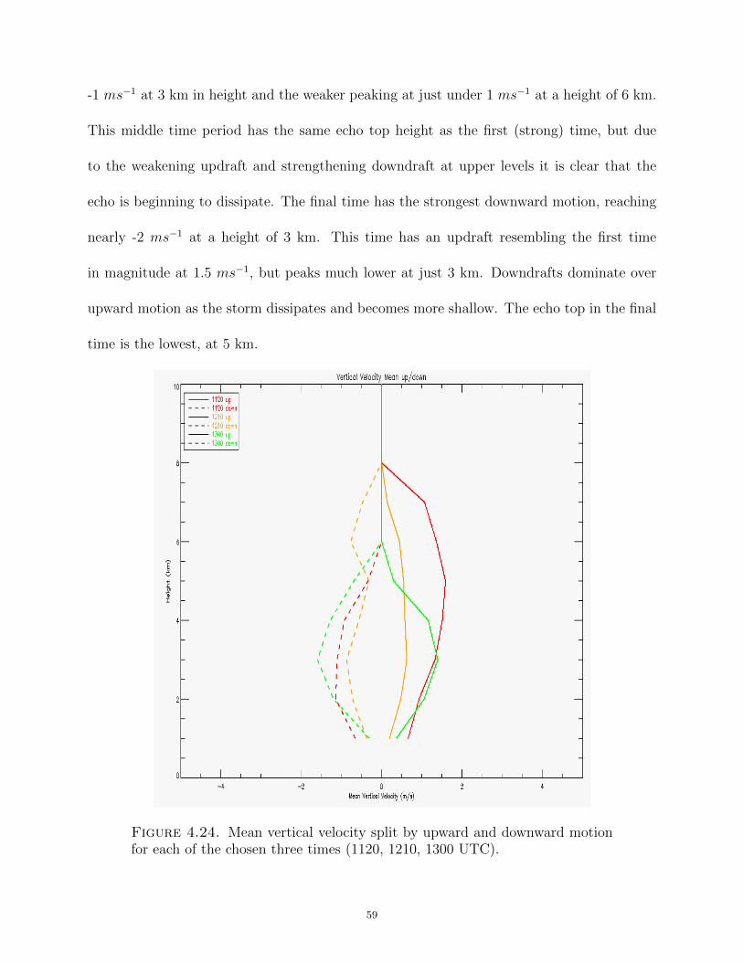
Splitting the vertical motion means between upward and downward motion can also
provide useful insight into the storm evolution. In figure 4.24, the first time of 1120 UTC
is dominated almost completely by upward motion at the top of the storm, with a small
contribution from the downward motion below. The upward motion peaks at just under 2
ms−1 at a height of 7.5 km. The next time has very little upward motion, and stays constant
at 0.5 ms−1 while the downdraft shows a double peak structure, with the strongest one being
58
-1 ms−1 at 3 km in height and the weaker peaking at just under 1 ms−1 at a height of 6 km.
This middle time period has the same echo top height as the first (strong) time, but due
to the weakening updraft and strengthening downdraft at upper levels it is clear that the
echo is beginning to dissipate. The final time has the strongest downward motion, reaching
nearly -2 ms−1 at a height of 3 km. This time has an updraft resembling the first time
in magnitude at 1.5 ms−1, but peaks much lower at just 3 km. Downdrafts dominate over
upward motion as the storm dissipates and becomes more shallow. The echo top in the final
time is the lowest, at 5 km.
Figure 4.24. Mean vertical velocity split by upward and downward motionfor each of the chosen three times (1120, 1210, 1300 UTC).
59
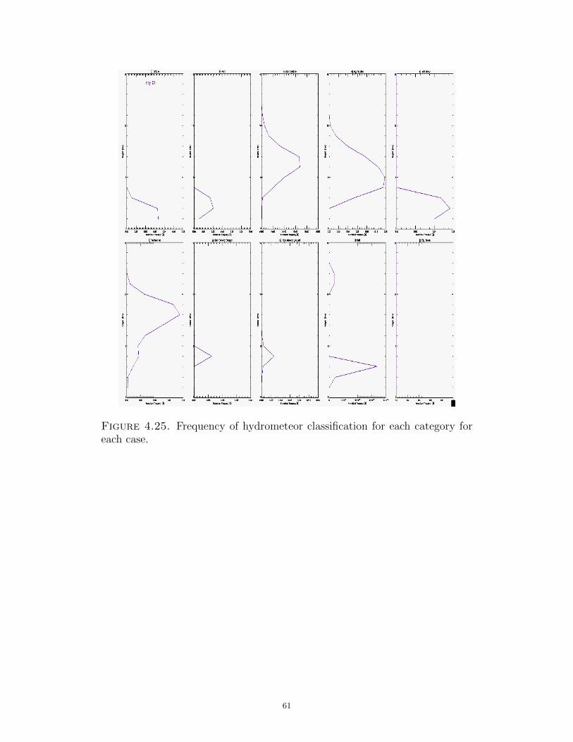
4.1.2.2. Microphysics. Finally, in the analysis of this case, we will examine the hydrom-
eteor classifications present. In figure 4.25, this case is shown in purple. The HID show rain
and drizzle at the surface, with ice crystals (IC), vertically oriented ice (VI) and aggregates
aloft. The vertical ice category is generally noted in strong electric fields in electrified con-
vection, which is not present in this case. However, later in the day from 16 UTC to 18 UTC,
convective storms moved through producing frequent lightning. The vertical ice noted at
this time may be due to a developing electrical charge in the atmosphere, or it may be a mis-
classification of the hydrometeor algorithm. Interestingly, wet snow is found not only to have
a peak at the height of the melting layer, as expected, but also to be present at the surface,
indicating that there may have been transitional season precipitation during this case. In the
MC3E research logs, a present scientist noted ’sleet’ falling at the surface. This confirms the
hypothesis that this day exhibited a transitional weather pattern, although ’sleet’ and ’wet
snow’ are not the same, and the log may not have occurred at the same time as the radar
indicated surface wet snow. The melting layer also contained a peak in low density graupel
and high density graupel, with the frequency of these extending upward toward the top of
the storm. The particles that reached the highest heights were aggregates, ice crystals, and
vertical ice, although vertical ice had the highest peak of these. Not surprisingly, there were
no big drops or hail found on this day due to the more stratiform nature of this case, and
the abundance of small ice particles aloft.
60
Figure 4.25. Frequency of hydrometeor classification for each category foreach case.
61
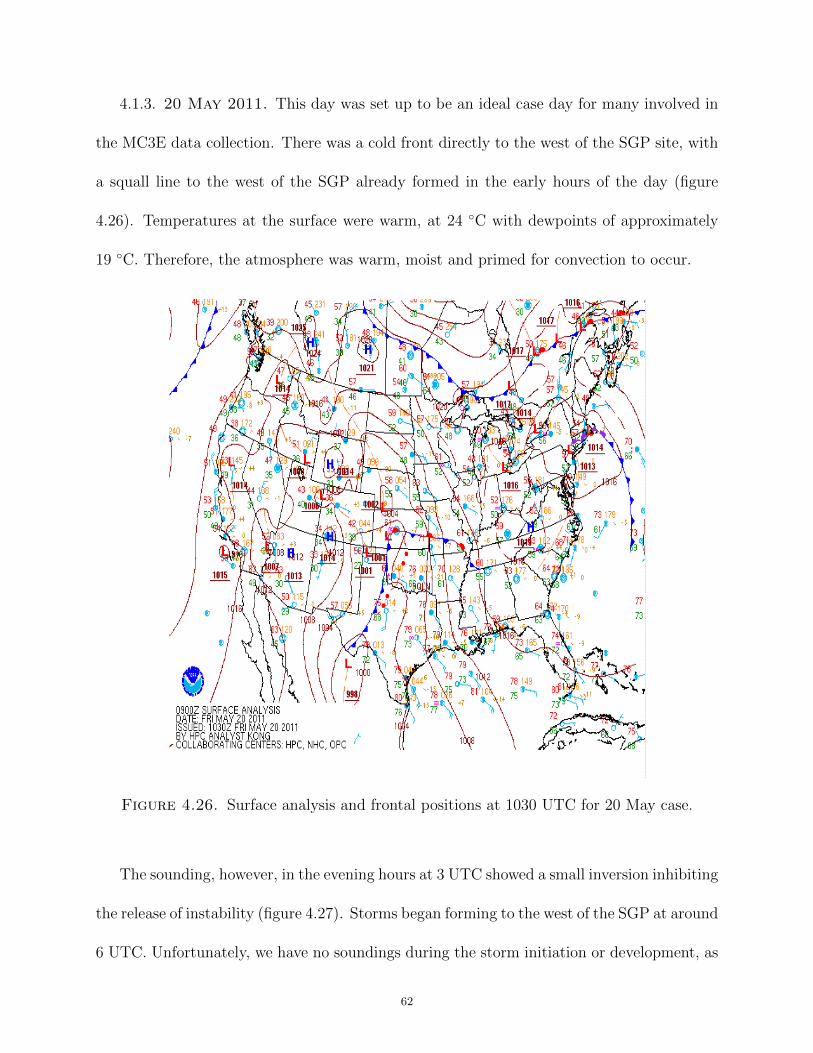
4.1.3. 20 May 2011. This day was set up to be an ideal case day for many involved in
the MC3E data collection. There was a cold front directly to the west of the SGP site, with
a squall line to the west of the SGP already formed in the early hours of the day (figure
4.26). Temperatures at the surface were warm, at 24 ◦C with dewpoints of approximately
19 ◦C. Therefore, the atmosphere was warm, moist and primed for convection to occur.
Figure 4.26. Surface analysis and frontal positions at 1030 UTC for 20 May case.
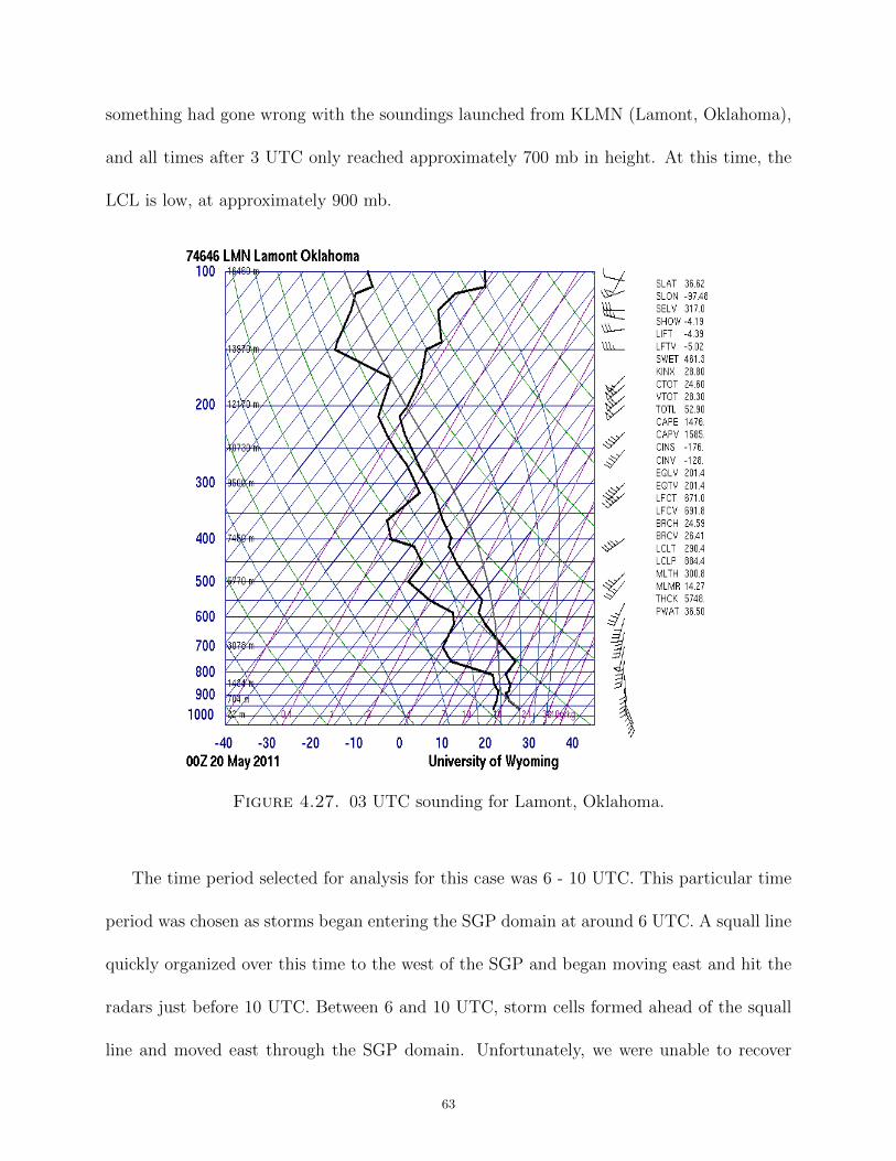
The sounding, however, in the evening hours at 3 UTC showed a small inversion inhibiting
the release of instability (figure 4.27). Storms began forming to the west of the SGP at around
6 UTC. Unfortunately, we have no soundings during the storm initiation or development, as
62
something had gone wrong with the soundings launched from KLMN (Lamont, Oklahoma),
and all times after 3 UTC only reached approximately 700 mb in height. At this time, the
LCL is low, at approximately 900 mb.
Figure 4.27. 03 UTC sounding for Lamont, Oklahoma.
The time period selected for analysis for this case was 6 - 10 UTC. This particular time
period was chosen as storms began entering the SGP domain at around 6 UTC. A squall line
quickly organized over this time to the west of the SGP and began moving east and hit the
radars just before 10 UTC. Between 6 and 10 UTC, storm cells formed ahead of the squall
line and moved east through the SGP domain. Unfortunately, we were unable to recover
63
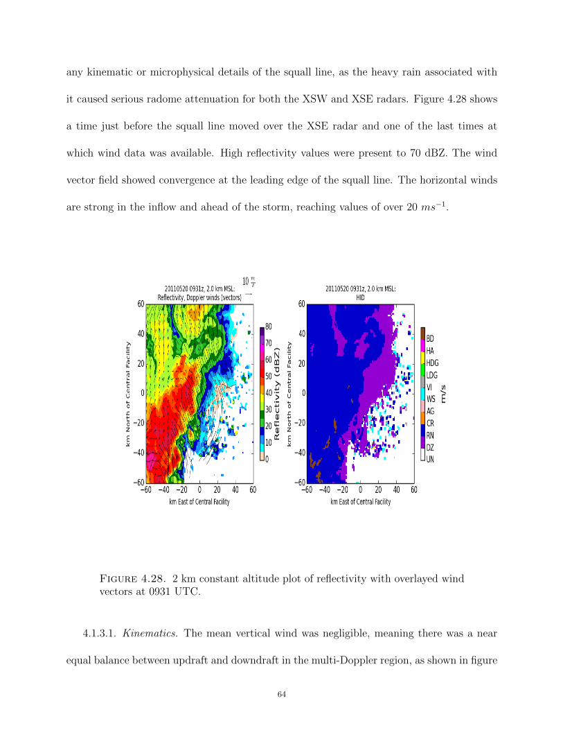
any kinematic or microphysical details of the squall line, as the heavy rain associated with
it caused serious radome attenuation for both the XSW and XSE radars. Figure 4.28 shows
a time just before the squall line moved over the XSE radar and one of the last times at
which wind data was available. High reflectivity values were present to 70 dBZ. The wind
vector field showed convergence at the leading edge of the squall line. The horizontal winds
are strong in the inflow and ahead of the storm, reaching values of over 20 ms−1.
Figure 4.28. 2 km constant altitude plot of reflectivity with overlayed windvectors at 0931 UTC.
4.1.3.1. Kinematics. The mean vertical wind was negligible, meaning there was a near
equal balance between updraft and downdraft in the multi-Doppler region, as shown in figure
64
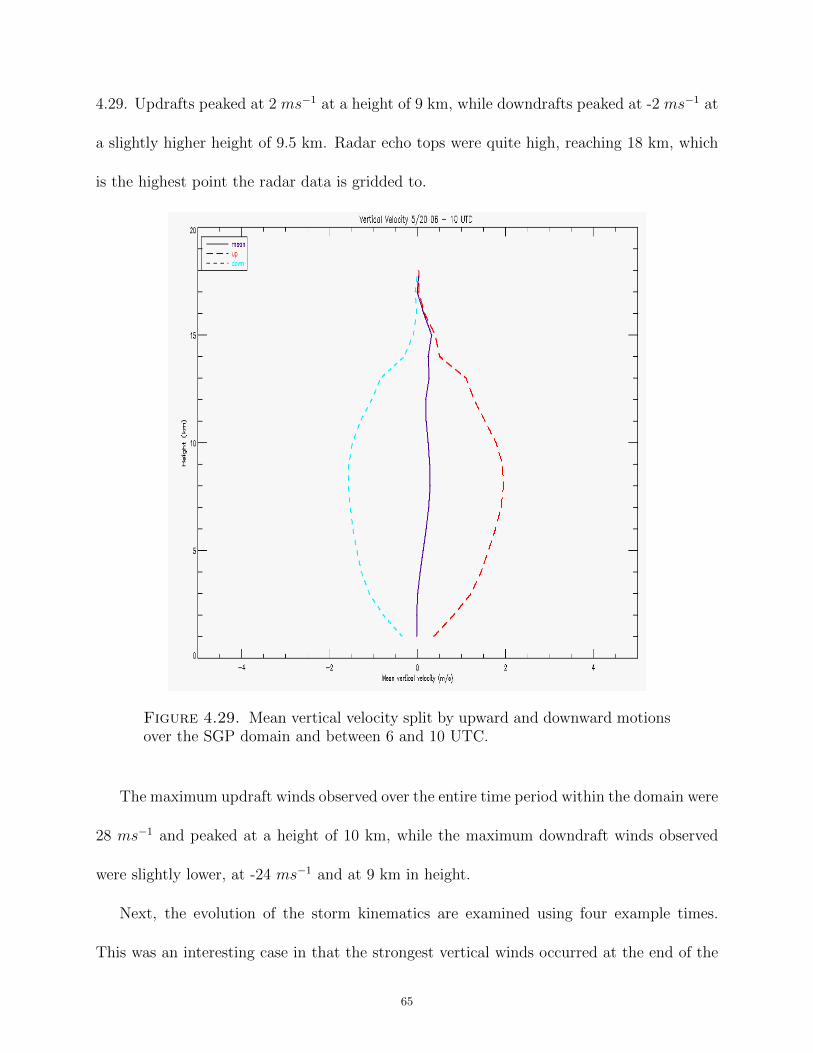
4.29. Updrafts peaked at 2 ms−1 at a height of 9 km, while downdrafts peaked at -2 ms−1 at
a slightly higher height of 9.5 km. Radar echo tops were quite high, reaching 18 km, which
is the highest point the radar data is gridded to.
Figure 4.29. Mean vertical velocity split by upward and downward motionsover the SGP domain and between 6 and 10 UTC.
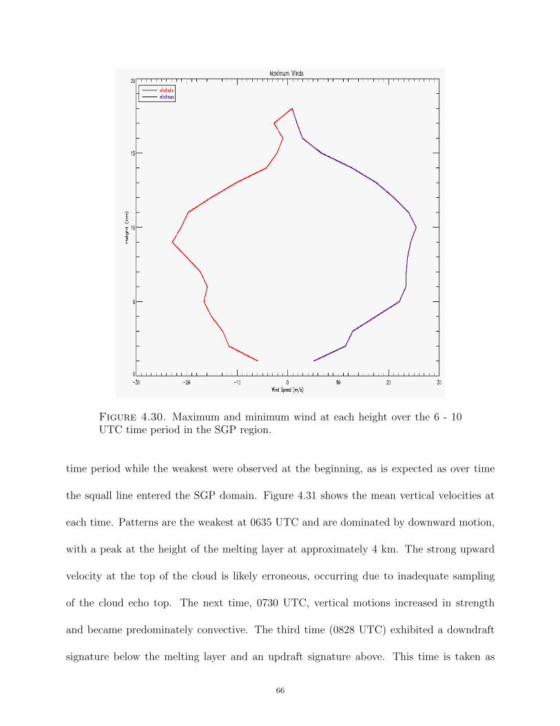
The maximum updraft winds observed over the entire time period within the domain were
28 ms−1 and peaked at a height of 10 km, while the maximum downdraft winds observed
were slightly lower, at -24 ms−1 and at 9 km in height.
Next, the evolution of the storm kinematics are examined using four example times.
This was an interesting case in that the strongest vertical winds occurred at the end of the
65
Figure 4.30. Maximum and minimum wind at each height over the 6 - 10UTC time period in the SGP region.
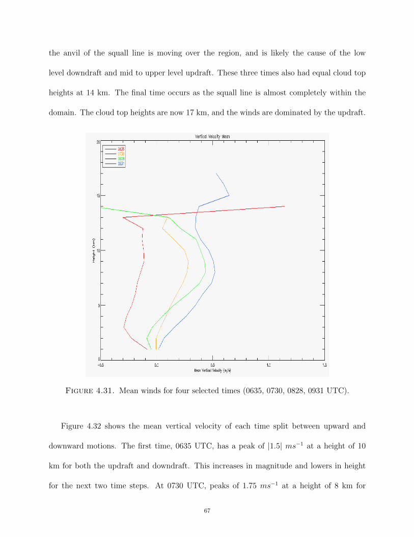
time period while the weakest were observed at the beginning, as is expected as over time
the squall line entered the SGP domain. Figure 4.31 shows the mean vertical velocities at
each time. Patterns are the weakest at 0635 UTC and are dominated by downward motion,
with a peak at the height of the melting layer at approximately 4 km. The strong upward
velocity at the top of the cloud is likely erroneous, occurring due to inadequate sampling
of the cloud echo top. The next time, 0730 UTC, vertical motions increased in strength
and became predominately convective. The third time (0828 UTC) exhibited a downdraft
signature below the melting layer and an updraft signature above. This time is taken as
66
the anvil of the squall line is moving over the region, and is likely the cause of the low
level downdraft and mid to upper level updraft. These three times also had equal cloud top
heights at 14 km. The final time occurs as the squall line is almost completely within the
domain. The cloud top heights are now 17 km, and the winds are dominated by the updraft.
Figure 4.31. Mean winds for four selected times (0635, 0730, 0828, 0931 UTC).
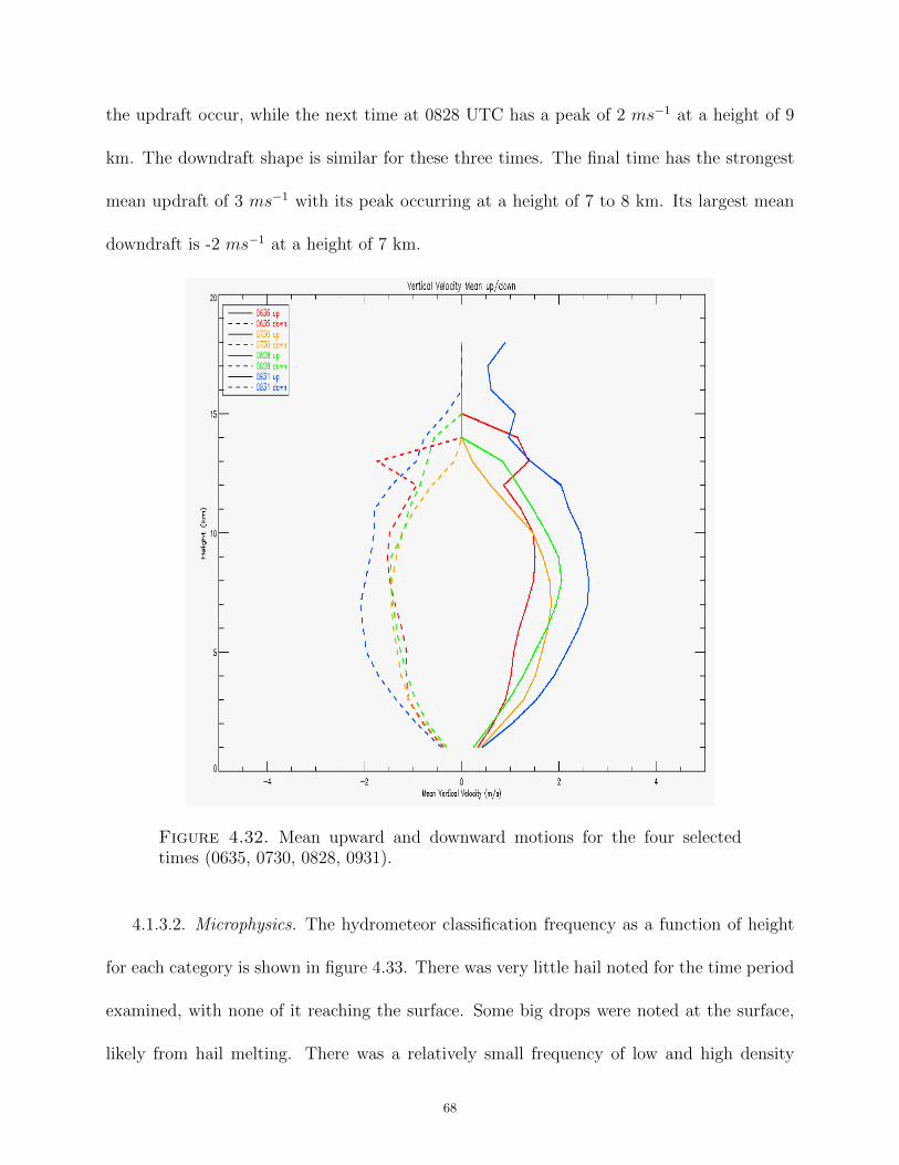
Figure 4.32 shows the mean vertical velocity of each time split between upward and
downward motions. The first time, 0635 UTC, has a peak of |1.5| ms−1 at a height of 10
km for both the updraft and downdraft. This increases in magnitude and lowers in height
for the next two time steps. At 0730 UTC, peaks of 1.75 ms−1 at a height of 8 km for
67
the updraft occur, while the next time at 0828 UTC has a peak of 2 ms−1 at a height of 9
km. The downdraft shape is similar for these three times. The final time has the strongest
mean updraft of 3 ms−1 with its peak occurring at a height of 7 to 8 km. Its largest mean
downdraft is -2 ms−1 at a height of 7 km.
Figure 4.32. Mean upward and downward motions for the four selectedtimes (0635, 0730, 0828, 0931).
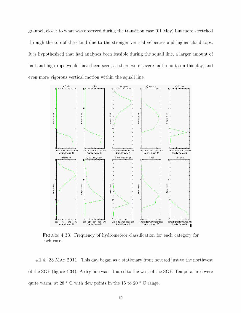
4.1.3.2. Microphysics. The hydrometeor classification frequency as a function of height
for each category is shown in figure 4.33. There was very little hail noted for the time period
examined, with none of it reaching the surface. Some big drops were noted at the surface,
likely from hail melting. There was a relatively small frequency of low and high density
68
graupel, closer to what was observed during the transition case (01 May) but more stretched
through the top of the cloud due to the stronger vertical velocities and higher cloud tops.
It is hypothesized that had analyses been feasible during the squall line, a larger amount of
hail and big drops would have been seen, as there were severe hail reports on this day, and
even more vigorous vertical motion within the squall line.
Figure 4.33. Frequency of hydrometeor classification for each category foreach case.
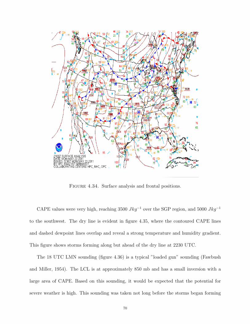
4.1.4. 23 May 2011. This day began as a stationary front hovered just to the northwest
of the SGP (figure 4.34). A dry line was situated to the west of the SGP. Temperatures were
quite warm, at 28 ◦ C with dew points in the 15 to 20 ◦ C range.
69
Figure 4.34. Surface analysis and frontal positions.
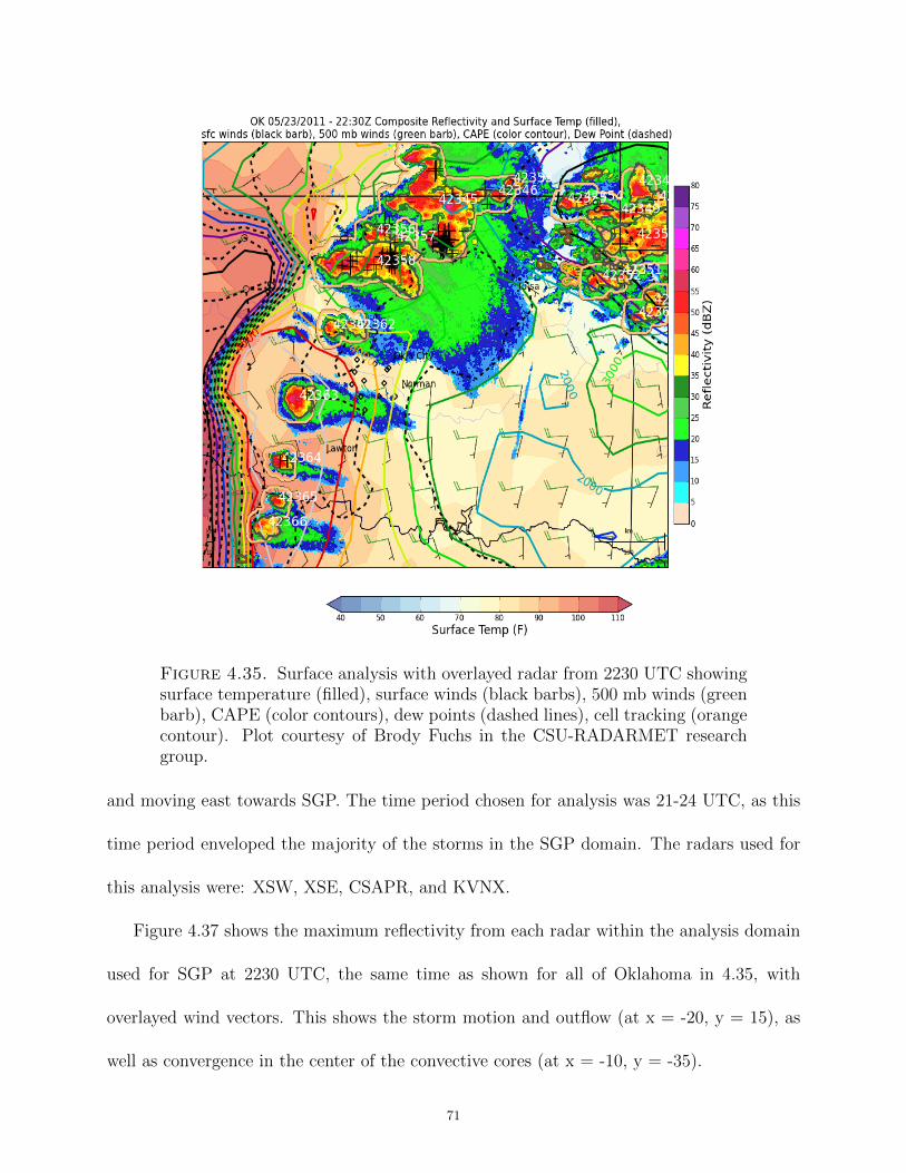
CAPE values were very high, reaching 3500 Jkg−1 over the SGP region, and 5000 Jkg−1
to the southwest. The dry line is evident in figure 4.35, where the contoured CAPE lines
and dashed dewpoint lines overlap and reveal a strong temperature and humidity gradient.
This figure shows storms forming along but ahead of the dry line at 2230 UTC.
The 18 UTC LMN sounding (figure 4.36) is a typical ”loaded gun” sounding (Fawbush
and Miller, 1954). The LCL is at approximately 850 mb and has a small inversion with a
large area of CAPE. Based on this sounding, it would be expected that the potential for
severe weather is high. This sounding was taken not long before the storms began forming
70
Figure 4.35. Surface analysis with overlayed radar from 2230 UTC showingsurface temperature (filled), surface winds (black barbs), 500 mb winds (greenbarb), CAPE (color contours), dew points (dashed lines), cell tracking (orangecontour). Plot courtesy of Brody Fuchs in the CSU-RADARMET researchgroup.
and moving east towards SGP. The time period chosen for analysis was 21-24 UTC, as this
time period enveloped the majority of the storms in the SGP domain. The radars used for
this analysis were: XSW, XSE, CSAPR, and KVNX.
Figure 4.37 shows the maximum reflectivity from each radar within the analysis domain
used for SGP at 2230 UTC, the same time as shown for all of Oklahoma in 4.35, with
overlayed wind vectors. This shows the storm motion and outflow (at x = -20, y = 15), as
well as convergence in the center of the convective cores (at x = -10, y = -35).
71
Figure 4.36. 18 UTC sounding for Lamont, Oklahoma for the 23 May case.
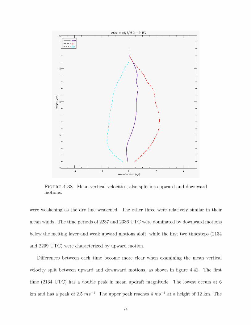
4.1.4.1. Kinematics. This case contained very strong vertical motion in the convective
cores, although this does not show up well in the means over the entire analysis period and
domain, as not everywhere had strong winds. These strongest winds were limited to the
supercellular storms. The mean vertical winds are shown in figure 4.38. The updraft has a
peak of 2.5 ms−1 at a height of 7 km, while the downdraft has a peak of just under 2 ms−1
at a height of 4 km. The overall mean is dominated slightly by the downdraft below the
melting layer and by the updraft above the melting layer.
72
Figure 4.37. CAPPI taken at 2 km at 2230 UTC showing reflectivity withoverlaying wind vectors.
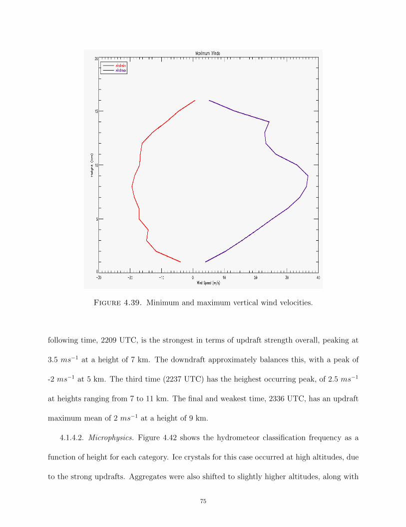
The maximum and minimum winds in figure 4.39 are quite impressive. The maximum
downward winds are relatively consistent throughout the troposphere, with a peak of -20
ms−1 at 8 km. The updraft maximum occurs at 9 km, up to 38 ms−1. The updraft is not
consistent with height, rather increasing nearly linearly with height to its peak value at 9
km.
Since storms moved so quickly through the SGP region, we chose to examine four different
storms. The vertical velocity means of these storm times (2134, 2209, 2237, 2336 UTC) are
shown in figure 4.40. The weakest of these storms was the final time analyzed, as storms
73
Figure 4.38. Mean vertical velocities, also split into upward and downwardmotions.
were weakening as the dry line weakened. The other three were relatively similar in their
mean winds. The time periods of 2237 and 2336 UTC were dominated by downward motions
below the melting layer and weak upward motions aloft, while the first two timesteps (2134
and 2209 UTC) were characterized by upward motion.
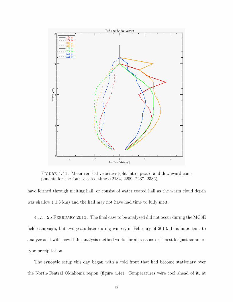
Differences between each time become more clear when examining the mean vertical
velocity split between upward and downward motions, as shown in figure 4.41. The first
time (2134 UTC) has a double peak in mean updraft magnitude. The lowest occurs at 6
km and has a peak of 2.5 ms−1. The upper peak reaches 4 ms−1 at a height of 12 km. The
74
Figure 4.39. Minimum and maximum vertical wind velocities.
following time, 2209 UTC, is the strongest in terms of updraft strength overall, peaking at
3.5 ms−1 at a height of 7 km. The downdraft approximately balances this, with a peak of
-2 ms−1 at 5 km. The third time (2237 UTC) has the heighest occurring peak, of 2.5 ms−1
at heights ranging from 7 to 11 km. The final and weakest time, 2336 UTC, has an updraft
maximum mean of 2 ms−1 at a height of 9 km.
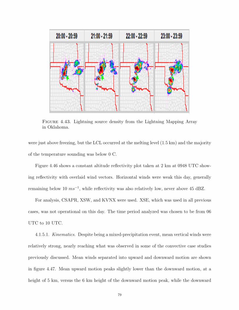
4.1.4.2. Microphysics. Figure 4.42 shows the hydrometeor classification frequency as a
function of height for each category. Ice crystals for this case occurred at high altitudes, due
to the strong updrafts. Aggregates were also shifted to slightly higher altitudes, along with
75
Figure 4.40. Mean vertical velocity for four selected time steps (2134, 2209,2237, 2336 UTC) on 23 May
vertical ice. Vertical ice also occurred in a very large volume due to the high electrification
of the storm leading to vertical alignment of ice crystals, with the lightning source density
shown in figure 4.43 is taken from the Oklahoma Lightning Mapping Array. High density
graupel occurred just above the melting layer, while low density graupel appears frequently
above the high density graupel peak. The most interesting aspect of this storm is the large
amount of hail aloft and big drops at the surface. There were severe hail reports this day, so
the presense of hail at the surface is physically reasonable. The big drops in this case may
76
Figure 4.41. Mean vertical velocities split into upward and downward com-ponents for the four selected times (2134, 2209, 2237, 2336)
have formed through melting hail, or consist of water coated hail as the warm cloud depth
was shallow ( 1.5 km) and the hail may not have had time to fully melt.
4.1.5. 25 February 2013. The final case to be analyzed did not occur during the MC3E
field campaign, but two years later during winter, in February of 2013. It is important to
analyze as it will show if the analysis method works for all seasons or is best for just summer-
type precipitation.
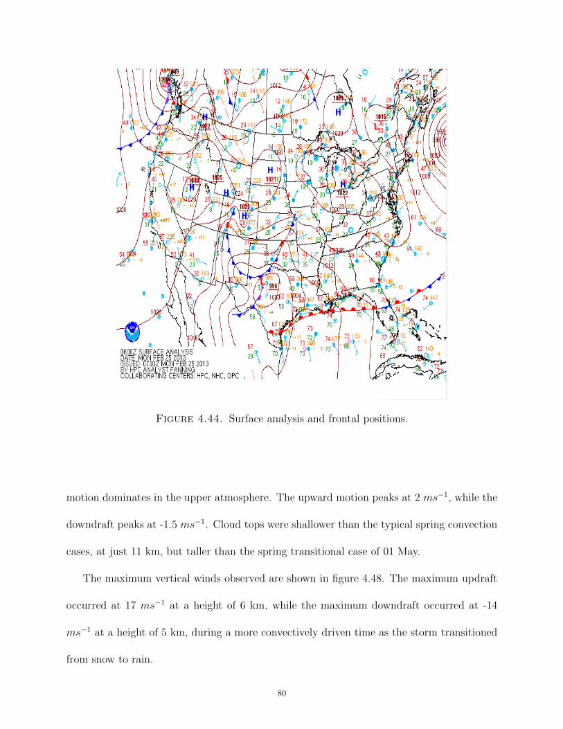
The synoptic setup this day began with a cold front that had become stationary over
the North-Central Oklahoma region (figure 4.44). Temperatures were cool ahead of it, at
77
Figure 4.42. Frequency of hydrometeor classification for each category foreach case. At this time, the red line depicting 23 May 2011 is of interest.
8 ◦ C with dewpoints of 0 ◦C, while behind the front it was slightly cooler and moister,
with temperatures of 3 ◦ C and dewpoints of 2.5 ◦ C. The SGP site was located right along
the stationary front and therefore experienced some mixed precipitation and snow, as was
evident from the Community Collaborative Rain, Hail & Snow Network (CoCoRahs), which
noted up to five inches of snow occurring on this day, although this did not occur during the
analysis period in which the required radars were running.
The LMN sounding taken at 12 UTC (figure 4.45), during an time of active precipitation,
was very moist. The LCL was low, at 900 mb, and there was no CAPE. Surface temperatures
78
Figure 4.43. Lightning source density from the Lightning Mapping Arrayin Oklahoma.
were just above freezing, but the LCL occurred at the melting level (1.5 km) and the majority
of the temperature sounding was below 0 C.
Figure 4.46 shows a constant altitude reflectivity plot taken at 2 km at 0948 UTC show-
ing reflectivity with overlaid wind vectors. Horizontal winds were weak this day, generally
remaining below 10 ms−1, while reflectivity was also relatively low, never above 45 dBZ.
For analysis, CSAPR, XSW, and KVNX were used. XSE, which was used in all previous
cases, was not operational on this day. The time period analyzed was chosen to be from 06
UTC to 10 UTC.
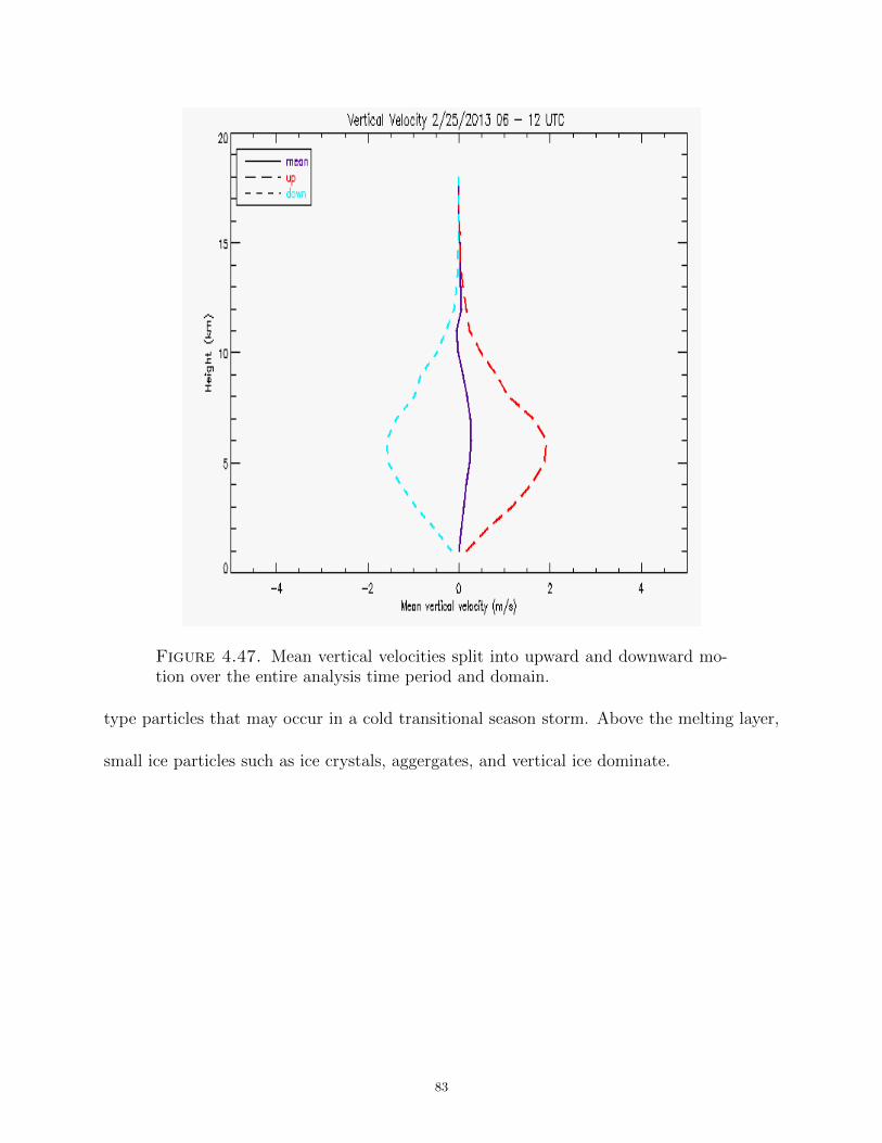
4.1.5.1. Kinematics. Despite being a mixed-precipitation event, mean vertical winds were
relatively strong, nearly reaching what was observed in some of the convective case studies
previously discussed. Mean winds separated into upward and downward motion are shown
in figure 4.47. Mean upward motion peaks slightly lower than the downward motion, at a
height of 5 km, versus the 6 km height of the downward motion peak, while the downward
79
Figure 4.44. Surface analysis and frontal positions.
motion dominates in the upper atmosphere. The upward motion peaks at 2 ms−1, while the
downdraft peaks at -1.5 ms−1. Cloud tops were shallower than the typical spring convection
cases, at just 11 km, but taller than the spring transitional case of 01 May.
The maximum vertical winds observed are shown in figure 4.48. The maximum updraft
occurred at 17 ms−1 at a height of 6 km, while the maximum downdraft occurred at -14
ms−1 at a height of 5 km, during a more convectively driven time as the storm transitioned
from snow to rain.
80
Figure 4.45. 12 UTC sounding for Lamont, Oklahoma.
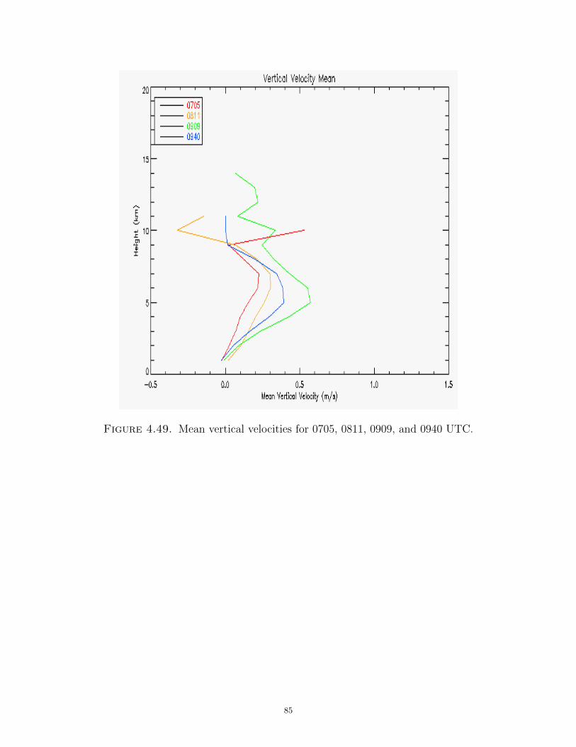
The four times chosen for further analysis were: 0705, 0811, 0909, and 0940 UTC. The
mean vertical velocities for these times can be seen in figure 4.49. All of the times chosen were
dominated by upward motion throught, with the strongest mean vertical winds occuring at
0909 UTC.
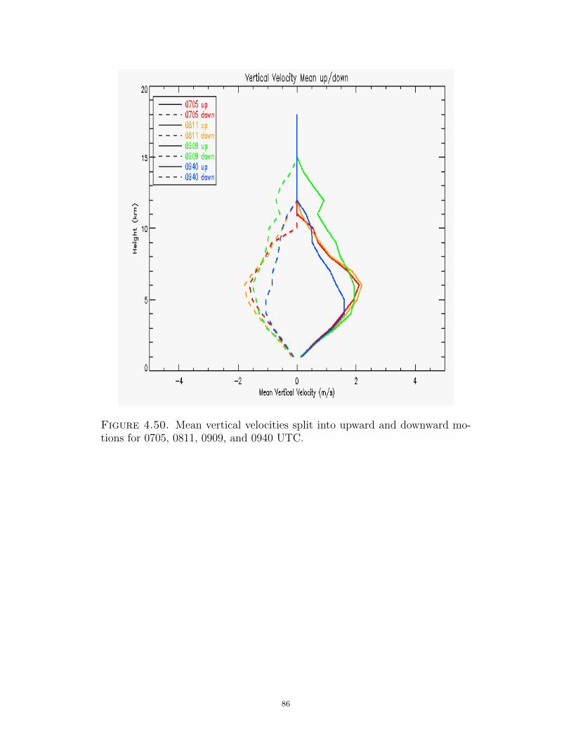
The vertical velocity means were then separated into their upward and downward compo-
nents, as shown in figure 4.50. The final time of 0940 UTC time is the weakest, but all times
are quite similar in shape and magnitude. 0909 UTC had slightly weaker winds than 0705
81
Figure 4.46. 2 km cappi showing reflectivity with overlying wind vectors at0948 UTC.
and 0811 UTC, but had taller echo top heights at 15 km. This is likely a more convectively
driven time than the other times analyzed in this way.
4.1.5.2. Microphysics. When examining the microphysics, we used the same HID classi-
fication algorithm used previously, as this was a transitional case with strong winds and had
the potential to support more spring convection type particles.
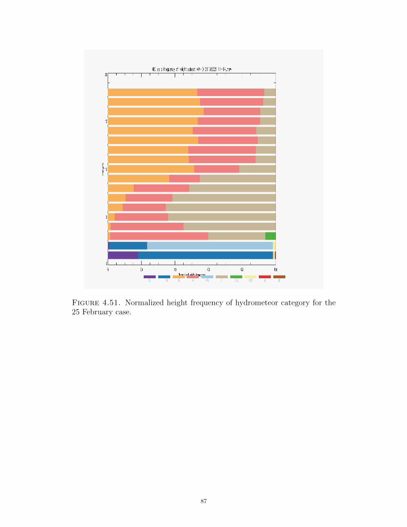
Figure 4.51 shows the frequency of each hydrometeor category at each height. Below the
low melting layer, mostly rain and drizzle are present. A small amount of hail, high density
graupel, and ice crystals are noted at the surface level. These are likely misclassified snow
82
Figure 4.47. Mean vertical velocities split into upward and downward mo-tion over the entire analysis time period and domain.
type particles that may occur in a cold transitional season storm. Above the melting layer,
small ice particles such as ice crystals, aggergates, and vertical ice dominate.
83
Figure 4.48. Maximum and minimum vertical wind speeds over the entireanalysis time period and domain.
84
Figure 4.49. Mean vertical velocities for 0705, 0811, 0909, and 0940 UTC.
85
Figure 4.50. Mean vertical velocities split into upward and downward mo-tions for 0705, 0811, 0909, and 0940 UTC.
86
Figure 4.51. Normalized height frequency of hydrometeor category for the25 February case.
87
CHAPTER 5
Conclusion
In this research, the kinematic and microphysical structures of multiple types of precipi-
tating events were analyzed using various datasets from the ARM-SGP site in North-Central
Oklahoma. The large number of instruments present during the Midlatitude Continental
Convective Clouds Campaign (MC3E) and provided by the ARM organization as perma-
nent installments allowed for multi-Doppler analysis using three to four radars, as well as a
multi-wavelength hydrometeor classification. The presence of the S-band profiler allowed for
validation of the multi-Doppler radar derived vertical winds to within 1 ms−1, and showed
that the downward motions may be undersampled by the radar derived method possibly due
to the difficulty the multi-Doppler method has in detecting low level divergence (Nelson and
Brown, 1987) due to the radar sampling missing the low levels of the atmosphere. A method
was also developed to allow analysis of multiple cases using the same methodology. Analysis
of a more wintery transitional precipitation event showed that the HID method used in con-
vective cases is applicable to transitional cases, although may misclassify ice particles below
the melting layer.
The consistent methodology applied to several cases that occurred during MC3E allows
for a unique opportunity to compare the different cases that occurred within a month of each
other. The first case discussed, 25 April 2011, consisted of organized elevated thunderstorms.
The 1 May case exhibited characteristics of an early spring transitional event. The 20 May
case analyzed was for storms forming ahead of a squall line, as well as the beginning of
the same squall line entering the SGP area. Finally, the 23 May case contained strong
88
thunderstorms, some of which were supercellular. This would help modelers improve their
models through comparison as a wide range of storm types were observed and analyzed with
similar methodology.
The kinematics of each of these cases differed wildly. Figure 5.1 shows the mean upward
and downward motions for each case over the entire domain and time period of each case.
The winds are limited to only where the radars topped the storms, requiring a minimum of
20 dBZ at the top of the storm in order for it to count as topped. This 20 dBZ threshold
was chosen to ensure the storms were completely topped and that no effects due to errors in
meeting the upper boundary conditions of the multi-Doppler wind retrieval were included
(Dolan and Rutledge (2010)). The 23 May case had the strongest winds and the tallest
storms, while the 1 May case had the weakest winds and storms with the least vertical
development. When examining these updrafts, the 23 May case mean vertical winds peaked
at 3 ms−1 at 6 km and stayed fairly consistently at approximately 3 km up to the top of the
storm. The 25 April case exhibited a more curved updraft profile, with a peak of 2.5 ms−1at
7 km. The 20 May case had the highest occurring peak at a height of 10 km, but had weaker
updrafts at 2 ms−1. The 1 May case updraft peaked at 1 ms−1 at 3 km. The downdraft
curves (dashed) are also quite different. The 23 May storm downdraft mean peaked low
in height, at 3 to 4 km, which was the melting layer height for this case, and had a speed
of nearly -2 ms−1, the strongest seen of all the cases analyzed. The 20 May case had the
second strongest downdrafts and the highest peak in mean downward motion, of -1.5 ms−1
at a height of 10 km. This case also has the most equally matched updraft and downdraft
regions, meaning that the storms were mostly mature storms and entering the beginning
89
dissipation stages. The 25 April case had consistent mean downward motion of -1.25 ms−1
peaking at 3 to 4 km and slowly weakening with height. Once again, the 1 May case is shown
to be more closely related to stratiform or winter precipitation, as its downdraft is stronger
than its updraft at the surface, at just over 1 ms−1 peaking at 3 km in height.
Figure 5.1. Multi-Doppler vertical wind means split into upward and down-ward motion for storms in which the radar topped up to at least 20 dBZ forall cases examined during MC3E.
The hydrometeor classifications of each storm are also different, as shown in figure 5.2.
The 23 May case has the largest volume of hail, which is logical as it also had the strongest
updraft and is able to support the development and growth of hail stones. It also had the
90
most vertical ice aloft, likely due to the large electrification of the storm seen in the previous
chapter. This case also had the highest occurring peak in high density graupel (4 km) and
low density graupel (5 km) owing to the presence of the strongest vertical winds. The 20
May case had the same melting layer height, but its weaker vertical winds were apparently
unable to support the formation of the high density or low density graupel as well ahead of
the squall line. A significantly lower hail frequency was also noted, although this was likely
due to being unable to conduct observations during the intense squall line phase. Both 23
May and 25 April have a high frequency of big drop occurrance. One possible formation
mechanism for this is melting hail. This is likely the situation for both cases, as both had
deep warm cloud depths for a surface lifted parcel. This would give plenty of time for the
hail to melt into large drops as it fell through this warm layer. In all cases, there was a
peak in high density graupel at or slightly above the melting layer. Low density graupel did
not peak for any case until after this peak in high density graupel had occurred and begun
decreasing.
Comparisons were done for the 25 April case between radar observations and simulations
from the WRF-SBM model. Both model and radar observations show reasonable agreement
for kinematic and microphysical characteristics of the storm. Both showed a peak updraft
occurring at 7 km in height, and a maximum reflectivity generally below 60 dBZ. However,
the model simulations showed stronger updraft maximums, higher reflectivities, and higher
echo tops, implying that the simulated convection was too strong for the weakly forced case.
The model and radar observations both exhibited weaker downdrafts generally remaining
below -10 ms−1 in both deep and shallow regimes, although the radar did show stronger
91
Figure 5.2. Frequency of classification for each hydrometeor category foreach case examined during MC3E.
downdrafts than the model. Examinations of the microphysical charactistics of the model
and radar observations revealed that the model classifies more graupel and snow aggregates
above 10 km, while the radar observations indicated mostly ice crystals in this region. The
model underestimated drizzle below the melting layer in shallow regimes, but in general the
model and radar observations agreed above the melting layer in areas of shallow convection.
These differences likely occurred due to the overlapping of several categories, such as low
and high density graupel, and small low density graupel vs aggregates.
92
The winter transitional precipitation case analyzed had weaker winds than most of the
convective spring cases, but stronger than the late spring transitional case of 1 May 2011. It
also had a low melting level with rain and ice particles below it and aggregates, ice crystals,
and vertical ice above. Modifications will need to be done to the methodology in order to
improve hydrometeor classifications for ice particles below the melting layer, which would
allow for further analysis of winter precipitation events using the radar network.
5.1. Future Work
The ARM-SGP facility offers an abundance of instruments, from scanning and profiling
radars to disdrometers, that would be useful for more detailed analysis of future storms
in the region. Oklahoma provides a chance to observe both strong storms in late spring,
pyrocumulus in summer from large wildfires, and transitional precipitation or snow in winter.
In the long term, the methodology developed in this research could be applied to all three
years of data, as well as all future cases that may occur. This would provide an idea of the
climatological changes occurring in the region, as well as the characterization of the general
climatology of precipitation and storms in the region from a kinematic and microphysical
perspective. The many wavelengths of precipitation radars present are ideal for achieving the
best hydrometeor classification available, as was shown in the multi-wavelength hydrometeor
identification algorithm based on Dolan et al. (2014). The presence of so many radars also
allows for an over-analyzed multi-Doppler wind retrieval over the region as well as comparison
to a profiling radar for validation.
All of the above mentioned benefits of the ample measurements available could provide a
better insight into the processes present in a wide variety of precipitation and clouds. These
93
measurements could then be compared to more model simulations to improve the model
analysis. A suggested future research would be to create a polarimetric radar emulator,
as this would be able to simulate polarimetric data based on cloud model outputs (such as
done by Ryzhkov et al. (2011)) that could then be run through the hydrometeor classification
algorithm for precipitation radars for a more direct comparison to radar based observational
analyses.
94
Bibliography
Baldini, L., E. Gorgucci, V. Chandrasekar, and W. Petersen, 2005: Implementations of csu
hydrometeor classification scheme for c-band polarimetric radars. Preprints, 32nd Conf.