EPA/600/R-06/097 September 2006 STORM WATER MANAGEMENT MODEL QUALITY ASSURANCE REPORT: Dynamic Wave Flow Routing By Lewis A. Rossman Water Supply and Water Resources Division National Risk Management Research Laboratory Cincinnati, OH 45268 NATIONAL RISK MANAGEMENT RESEARCH LABORATORY OFFICE OF RESEARCH AND DEVELOPMENT U.S. ENVIRONMENTAL PROTECTION AGENCY CINCINNATI, OH 45268
Transcript
EPA/600/R-06/097
September 2006
STORM WATER MANAGEMENT MODEL
QUALITY ASSURANCE REPORT:
Dynamic Wave Flow Routing
By
Lewis A. Rossman Water Supply and Water Resources Division
National Risk Management Research Laboratory Cincinnati, OH 45268
NATIONAL RISK MANAGEMENT RESEARCH LABORATORY OFFICE OF RESEARCH AND DEVELOPMENT
U.S. ENVIRONMENTAL PROTECTION AGENCY CINCINNATI, OH 45268
ii
DISCLAIMER
The information in this document has been funded wholly or in part by the U.S. Environmental Protection Agency (EPA). It has been subjected to the Agency’s peer and administrative review, and has been approved for publication as an EPA document. Mention of trade names or commercial products does not constitute endorsement or recommendation for use.
iii
FOREWORD The U.S. Environmental Protection Agency is charged by Congress with protecting the Nation’s land, air, and water resources. Under a mandate of national environmental laws, the Agency strives to formulate and implement actions leading to a compatible balance between human activities and the ability of natural systems to support and nurture life. To meet this mandate, EPA’s research program is providing data and technical support for solving environmental problems today and building a science knowledge base necessary to manage our ecological resources wisely, understand how pollutants affect our health, and prevent or reduce environmental risks in the future.
The National Risk Management Research Laboratory is the Agency’s center for investigation of technological and management approaches for reducing risks from threats to human health and the environment. The focus of the Laboratory’s research program is on methods for the prevention and control of pollution to the air, land, water, and subsurface resources; protection of water quality in public water systems; remediation of contaminated sites and ground water; and prevention and control of indoor air pollution. The goal of this research effort is to catalyze development and implementation of innovative, cost-effective environmental technologies; develop scientific and engineering information needed by EPA to support regulatory and policy decisions; and provide technical support and information transfer to ensure effective implementation of environmental regulations and strategies.
Water quality impairment due to runoff from urban and developing areas continues to be a major threat to the ecological health of our nation’s waterways. The EPA Storm Water Management Model is a computer program that can assess the impacts of such runoff and evaluate the effectiveness of mitigation strategies. This report documents the Quality Assurance testing that was performed on the dynamic wave flow routing portion of the recently modernized and updated version 5.0 of the model. As a result of this testing, users can have confidence that the updated model is performing correctly.
Sally C. Gutierrez, Director National Risk Management Research Laboratory
Appendix A. SWMM 4 Routing Models................................................................ 112
Appendix B. Test Data Sets .................................................................................... 115
5
1. Introduction The Storm Water Management Model (SWMM) was originally developed in 1971 as a computer-based tool for simulating storm water runoff quantity and quality from primarily urban areas (Metcalf & Eddy, Inc., et al., 1971). Since then it has undergone several major updates, the last of these being Version 4.4 (Huber and Dickinson, 1992) which is available through an Oregon State University web site (http://ccee.oregonstate.edu/swmm/). Throughout each of these updates the general block nature of the overall program as well as the basic structure of its Fortran source code has remained more or less intact. In 2002, the U.S. Environmental Protection Agency’s Water Supply and Water Resources Division partnered with the consulting firm CDM to develop a completely re-written version of SWMM. The goal of this project was to apply modern software engineering techniques to produce a more maintainable, extensible, and easier to use model. The result of this effort, SWMM 5 (Rossman, 2005), consists of a platform-independent computational engine written in C as well as a graphical user interface for the Microsoft Windows operating system written in Delphi. A rigorous Quality Assurance (QA) program was developed to insure that the numerical results produced from the new SWMM 5 model would be compatible with those obtained from SWMM 4.4 (Schade, 2002). The new SWMM 5 software was released to the public in October of 2004. The most numerically challenging sub-model to implement within SWMM 5 was the dynamic wave flow routing routine known as Extran (for Extended Transport). It routes non-steady flows through a general network of open channels, closed conduits, storage facilities, pumps, orifices and weirs. In contrast to simpler routing methods, this procedure can model such phenomena as backwater effects, flow reversals, pressurized flow, and entrance/exit energy losses. Rather than simply encode a line-for-line copy of Extran, SWMM 5 restructured the code in a more readable and maintainable fashion. It also employed a slightly modified computational scheme with the intent of producing more numerically stable solutions in less time. This report documents the Quality Assurance testing program that was used to compare the dynamic wave flow routing procedures of SWMM 4.4 and SWMM 5 with one another. Before describing the tests made and the results obtained it will be useful to contrast the way in which each version of the model implements dynamic wave flow routing.
6
2. Routing Models It should be noted that SWMM 4.4 (hereafter referred to as simply SWMM 4) actually contains three different procedures that can be used for dynamic wave flow routing. The choice is determined by the value of the ISOL parameter provided by the user in SWMM 4’s input data file. The Explicit Method (ISOL = 0) is the default and will be the method compared against in this report. Appendix A discusses this decision in more detail. Governing Equations Both SWMM 4 and 5 solve the same form of the conservation of mass and momentum equations that govern the unsteady flow of water through a drainage network of channels and pipes. These equations, known as the Saint Venant equations, can be expressed in the following form for flow along an individual conduit:
0=∂∂
+∂∂
xQ
tA Continuity (1)
0)/( 2
=++∂∂
+∂
∂+
∂∂
Lf gAhgASxHgA
xAQ
tQ Momentum (2)
where x is distance along the conduit, t is time, A is cross-sectional area, Q is flow rate, H is the hydraulic head of water in the conduit (elevation head plus any possible pressure head), Sf is the friction slope (head loss per unit length), hL is the local energy loss per unit length of conduit, and g is the acceleration of gravity. Note that for a known cross-sectional geometry, the area A is a known function of flow depth y which in turn can be obtained from the head H. Thus the dependent variables in these equations are flow rate Q and head H, which are functions of distance x and time t. The friction slope Sf can be expressed in terms of the Manning equation as:
3/42
2
RkVVn
S f =
where n is the Manning roughness coefficient, V is the flow velocity (equal to the flow rate Q divided by the cross-sectional area A), R is the hydraulic radius of the flow’s cross-section, and k = 1.49 for US units or 1.0 for metric units. The local loss term hL can be
expressed asgL
KV2
2
where K is a local loss coefficient at location x and L is the conduit
length. To solve equations (1) and (2) over a single conduit, one needs a set of initial conditions for H and Q at time 0 as well as boundary conditions at x = 0 and x = L for all times t.
7
When analyzing a network of conduits, an additional continuity relationship is needed for the junction nodes that connect two or more conduits together (see Figure 1.1). In SWMM a continuous water surface is assumed to exist between the water elevation at the node and in the conduits that enter and leave the node (with the exception of free fall drops should they occur). The change in hydraulic head H at the node with respect to time can be expressed as:
∑∑
+=
∂∂
AsAstoreQ
tH (3)
where Astore is the surface area of the node itself, ΣAs is the surface area contributed by the conduits connected to the node, and ΣQ is the net flow into the node (inflow – outflow) contributed by all conduits connected to the node as well as any externally imposed inflows. Note that the flow depth at the end of a conduit connected to a node can be computed as the difference between the head at the node and the invert elevation of the conduit.
Figure 1.1 Node-Link Representation of a Drainage System in SWMM (from
Roesner et al, 1992). General Solution for Conduits Equations (1), (2), and (3) are solved in SWMM by converting them into an explicit set of finite difference formulas that compute the flow in each conduit and head at each node for time t + ∆t as functions of known values at time t. The equation solved for the flow in each conduit is:
8
lossesfriction
inertialgravityttt QQ
QQQQ
∆+∆+
∆+∆+=∆+ 1
(4)
The individual ∆Q terms have been named for the type of force they represent and are given by the following expressions:
( ) LtHHAgQgravity /21 ∆−=∆
( ) ( ) LtAAVAAVQ tinertial /2 122 ∆−+−=∆
3/42
2
RktVgn
Q friction
∆=∆
L
tVKQ i
ii
losses 2
∆=∆
∑
where:
A = average cross-sectional flow area in the conduit, R = average hydraulic radius in the conduit, V = average flow velocity in the conduit, Vi = local flow velocity at location i along the conduit, Ki = local loss coefficient at location i along the conduit, H1 = head at upstream node of conduit, H2 = head at downstream node of conduit, A1 = cross-sectional area at the upstream end of the conduit, A2 = cross-sectional area at the downstream end of the conduit.
The equation solved for the head at each node is:
( )tt
ttt AsAstoreVolHH
∆+
∆+ ∑+∆
+= (5)
where ∆Vol is the net volume flowing through the node over the time step as given by:
( ) ( )[ ] tQQVolttt
∆+=∆∆+∑∑5.0
SWMM 4 solves equations (4) and (5) using the modified Euler method (equivalent to a 2nd order Runge-Kutta method). First Eq. (4) is solved for new flows in each conduit over a half time step ∆t/2 using the heads, areas, and velocities last computed for time t. The resulting flows are substituted into Eq. (5) to compute heads, using a time step of ∆t/2.
9
Then full-step flows are found by evaluating Eq. (4) again, this time using the full time step ∆t and using the heads, areas, and velocities found for the half-step solution. Finally, new heads for the full time step ∆t are found by solving Eq. (5) once more with the full-step flows. SWMM 5 solves equations (4) and (5) using a method of successive approximations with under relaxation. The procedure goes as follows: 1. A first estimate of flow in each conduit at time t+∆t is made by solving Eq. (4) using
the heads, areas, and velocities found at the current time t. Then the same is done for heads by evaluating Eq. (5) using the flows just computed. These solutions are denoted as Qlast and Hlast.
2. Eq. (4) is solved once again, using the heads, areas, and velocities that belong to the Qlast and Hlast values just computed. A relaxation factor Ω is used to combine the new flow estimate Qnew, with the previous estimate Qlast according to the equation
newlastnew QQQ Ω+Ω−= )1( to produce an updated value of Qnew. 3. Eq. (5) is solved once again for heads, using the flows Qnew. As with flow, this new
solution for head, Hnew, is weighted with Hlast to produce an updated estimate for heads, newlastnew HHH Ω+Ω−= )1( .
4. If Hnew is close enough to Hlast then the process stops with Qnew and Hnew as the solution for time t+∆t. Otherwise, Hlast and Qlast are replaced with Hnew and Qnew, respectively, and the process returns to step 2.
In implementing this procedure, SWMM 5 uses a constant relaxation factor Ω of 0.5, a convergence tolerance of 0.005 feet on nodal heads, and limits the number of trials to four. Computation of Average Conduit Conditions Evaluation of the flow updating Eq. (4) requires values for the average area ( A ), hydraulic radius ( R ), and velocity (V ) throughout the conduit in question. Both SWMM 4 and 5 compute these values using the heads H1 and H2 at either end of the conduit from which corresponding flow depth values y1 and y2 can be derived. An average depth y is then computed by averaging these values and is used with the conduit’s cross-section geometry to compute the average area A and hydraulic radius R . The average velocity V is found by dividing the most current flow value by the average area. SWMM 5 follows SWMM 4’s practice of limiting this velocity to be no higher than 50 ft/sec in absolute value, so as not to allow the frictional flow adjustment term in Eq. (4) to become unbounded. When the conduit has a free-fall discharge into either of its end nodes (meaning that the water elevation in the node is below the invert elevation of the conduit), the depth at that end of the conduit is set equal to the smaller of the critical depth and the normal flow depth for the current flow through the conduit.
10
Computation of Surface Area The surface area As that conduits contribute to their end nodes is computed the same way in both SWMM 4 and 5 and depends on the flow condition within the conduit. Under normal conditions it equals half the conduit’s length times the average of the top width at the end- and mid-points of the conduit. These widths are evaluated before the next updated flow solution is found, using the flow depths y1, y2, and y discussed previously. If the conduit’s inflow to a node is in free-fall (i.e., the conduit invert is above the node’s water surface), then the conduit contributes nothing to the node’s surface area. For conduits with closed cross-sectional shapes (such as circular pipes) that are greater than 96 percent full, SWMM 4 utilizes a constant top width equal to the width when 96 percent full. This prevents the head adjustment term in Eq. (5) from blowing up as the actual top width and corresponding surface area go to 0 as the conduit approaches being full. This same practice is followed in SWMM 5. Both programs assign a minimum surface area Astoremin to all nodes, including junctions that normally have no storage volume, to prevent Eq. (5) from becoming unbounded. The default value for this minimum area is 12.57 ft2 (i.e., the area of a 4-foot diameter manhole) but can be overridden by a user-supplied value. Surcharge Conditions SWMM defines a node to be in a surcharged condition when its water level exceeds the crown of the highest conduit connected to it. Under this condition the surface area contributed by any closed conduits would be zero and Eq. (3) would no longer be applicable. To accommodate this situation, SWMM uses an alternative nodal continuity condition, namely that the total rate of outflow from a surcharged node must equal the total rate of inflow, ΣQ = 0. By itself, this equation is insufficient to update nodal heads at the new time step since it only contains flows. In addition, because the flow and head updating equations for the system are not solved simultaneously, there is no guarantee that the condition will hold at the surcharged nodes after a flow solution has been reached. To enforce the flow continuity condition, it can be expressed in the form of a perturbation equation:
0=⎥⎦⎤
⎢⎣⎡ ∆
∂∂
+∑ HHQQ
where ∆H is the adjustment to the node’s head that must be made to achieve flow continuity. Solving for ∆H yields:
∑∑
∂∂
−=∆
HQQ
H/
(6)
11
where from Eq. (4),
lossesfriction QQLtAg
HQ
∆+∆+∆−
=∂∂
1/
( HQ ∂∂ has a negative sign in front of it because when evaluating ΣQ, flow directed out of a node is considered negative while flow into the node is positive.) Every time that Eq. (6) is applied to update the head at a surcharged node, Eq. (4) is re-evaluated to provide flow updates for the conduits that connect to the node. This process continues until some convergence criterion is met. SWMM 4 enters this iterative mode for surcharged nodes at both the half-step and full-step portions of its solution method. The user sets a convergence tolerance on the maximum fractional difference for flows found between iterations as well as the maximum number of iterations allowed. For SWMM 5, these surcharge iterations are folded into its normal set of iterations outlined previously. That is, whenever heads need to be computed in the successive approximation scheme, Eq. (6) is used in place of Eq. (5) if a node is surcharged, and no under-relaxation of the resulting head value is performed. Normal Flow Condition Both SWMM 4 and SWMM 5 limit the flow in non-surcharged conduits to be no greater than the normal Manning’s flow for the current flow depth at the upstream end of the conduit whenever one of the following conditions occur:
1. The water surface slope is less than the conduit slope. 2. The Froude number, based on the water depth at either end of the conduit, is
greater than 1.0. Each condition indicates a flow regime that is supercritical. The user specifies which of these two criteria should apply. Pumps, Orifices, and Weirs Both programs model pumps, orifices, and weirs as links that connect a pair of nodes together. The flow through these links is computed as a function of the heads at their end nodes. These flows are computed during the flow evaluation step of both the SWMM 4 and 5 procedures after the flows through all of the conduits are computed. SWMM 4 and 5 model pumps in a similar fashion, requiring the user to specify a pump curve along which the pump must operate. The pump curve can specify flow as a function of inlet node volume, inlet node depth, or the head difference between the inlet and outlet nodes. Both programs also limit the pump’s flow to the inflow to the inlet node during a given time step should the pump curve flow be high enough to completely drain the inlet node during the time step.
12
SWMM 4 models an orifice (i.e., an enclosed opening oriented either vertically or horizontally to the flow direction) as an equivalent pipe. The length L of the equivalent pipe is computed as gDt∆2 where D is the height of the orifice opening. Its roughness
coefficient is set equal to LgCR d 23/2 where R is the hydraulic radius of the full orifice opening and Cd is the discharge coefficient of the orifice. Flow through the orifice is then computed in the same fashion as for any conduit. SWMM 5 takes a more direct approach. It uses the classical orifice equation ghACd 2 to compute flow when the orifice is fully
submerged and a modified weir equation 5.12 fgDACd when the orifice is submerged a fraction f. In these formulas, A is the area and D is the height of the full orifice opening, while h is the head across the orifice. Both programs compute a surface area contribution of the orifice to its end nodes, based on the equivalent pipe length L and the depth of water in the orifice. SWMM 5 models weirs (i.e., an unrestricted opening oriented either transversely or parallel to the flow direction) in the same fashion as SWMM 4. An equation of the general form n
ww hLC is used to compute flow as a function of head h across the weir when the weir is not fully submerged. Cw is the weir’s discharge coefficient, Lw is the length of its opening, and n is an exponent that depends on the type of weir being modeled (e.g., transverse, side-flow, V-notch, or trapezoidal). When the weir becomes completely submerged, both programs switch to using the orifice equation to predict flow as a function of the head across it. Weirs do not contribute any surface area to their end nodes.
13
3. Testing Procedure The testing procedure used for this study involved running both SWMM 4 and 5 on an identical set of dynamic wave flow routing test problems and then comparing the results. Equivalent sets of analysis options, such as routing time step and minimum nodal surface area, were used with each program to maintain comparability (see below). The results produced by each program were inspected in the following ways: For examples that included a runoff calculation, the overall flow balances for runoff
were compared to make sure that both versions of SWMM produced the same total inflow quantities to the flow routing computation.
The flow balance error for the routing portion of each example was checked to insure that both versions of SWMM maintained acceptable flow continuity.
Scatter plots were used to visually compare the peak flows computed for all conduits in each example by each of the programs.
Time series plots of flows and water depths at critical locations in each example were visually compared, paying particular attention to any evidence of numerical instability exhibited by either program.
The critical locations chosen for time series plots typically included system outfalls, other significant system elements (such as orifices, weirs, storage units and pump stations), and locations that exhibited significant differences in peak flows between the two programs. The test case examples used in this evaluation were divided into three distinct categories. The first category is the Extran Manual Test Cases. These consist of the ten Extran example data sets that were presented in the last SWMM 4.4 Users Manual (Roesner et al., 1992). They serve as a useful benchmark to compare against and model such elements as surcharged conduit flow, bottom and side orifices, weirs, storage units, pumps, and a variety of cross-sectional shapes. The second test case category is the Challenge Test Cases. These are five examples from a suite of test cases compiled by Robert E. Dickinson of CDM. They all consist of several circular conduits connected in series that present different types of challenges to modeling dynamic flows, such as flat slopes, pipe constrictions, steep drops, adverse slopes, and inlet offsets. The third test category is the User Submitted Test Cases. These contain five real-world data sets contributed by SWMM users. They include models of either storm sewer systems, combined sewer systems or natural channel systems and range in size from 59 conduits up to 273 conduits. Each of these user examples includes a runoff component that generates the flows supplied to the routing component of the model. The versions of SWMM used in this comparison study were SWMM 4.4h (July 4, 2005) and SWMM 5.0.006 (September 2005). Unless otherwise indicated, the option settings listed in Table 3.1 were used in all runs to maintain computational compatibility between the two versions of SWMM. Note that the SWMM 4 ITMAX and SURTOL settings are not directly comparable to the SWMM 5 settings for maximum iterations and
14
convergence tolerance since the former apply only to surcharge iterations while the latter are used throughout SWMM 5’s successive approximation routine. Table 3.1. Computational Settings Used for the Test Case Comparisons. SWMM 4 SWMM 5 Setting Meaning Value Setting ValueISOL Solution method 0 Inertial terms KeepKSUPER Normal flow limit criterion 0 Normal flow limit criterion SlopeNEQUAL Lengthen short conduits 0 Lengthen short conduits NoAMEN Minimum surface area, ft2 12.57 Minimum surface area, ft2 12.57ITMAX Maximum iterations
(for surcharge only) 30 Maximum iterations
(fixed internally) 4
SURTOL Surcharge tolerance, expressed as a fractional flow difference
0.05 Convergence tolerance, expressed as an absolute head difference in feet (fixed internally)
0.005
15
4. Extran Manual Test Cases Example EXTRAN1 The drainage network used in this example is displayed in Figure 4.1. It contains 7 circular conduits arranged in 2 branches that converge into a pair of trapezoidal channels with a free outfall. Three locations as shown in the figure are subjected to the inflow hydrographs shown in Figure 4.2. The system was designed so that conduits 8040, 8060, and 1602 along the top branch become surcharged and flooding occurs at node 80608. It was analyzed using a 20 second time step over an 8 hour simulation period. SWMM 4 and 5 produced essentially identical results for this example. Comparison plots for flow in selected conduits and water depth at selected nodes are shown in Figures 4.3 through 4.6. The maximum flow at each conduit and the maximum water elevation at each node are compared in Figures 4.7 and 4.8, respectively.
80408060
81008130
1030
1570
1600
1630
1602 8040880608
8100981309
82309
10309 1500916009
16109
10208
EXAMPLE 1 OF EXTRAN MANUAL
InflowInflow
Inflow
Figure 4.1. Schematic of the Drainage Network Used for Example EXTRAN1.
16
0
10
20
30
40
50
60
0 1 2 3 4
Time (hours)
Inflo
w (c
fs)
Link 8040 Link 1602 Link 8100
Figure 4.2. External Inflows for Example EXTRAN1.
Link 1602 FlowSWMM5 SWMM4
Elapsed Time (hours)9876543210
Flow
(CFS
)
80.0
70.0
60.0
50.0
40.0
30.0
20.0
10.0
0.0
Figure 4.3. Flow Comparison for Link 1602 of Example EXTRAN1.
17
Link 1030 FlowSWMM5 SWMM4
Elapsed Time (hours)9876543210
Flow
(CFS
)
140.0
120.0
100.0
80.0
60.0
40.0
20.0
0.0
Figure 4.4. Flow Comparison for Link 1030 of Example EXTRAN1.
Node 82309 DepthSWMM5 SWMM4
Elapsed Time (hours)9876543210
Dept
h (f
t)
25.0
20.0
15.0
10.0
5.0
0.0
Figure 4.5. Water Depth Comparison for Node 82309 of Example EXTRAN1.
18
Node 16009 DepthSWMM5 SWMM4
Elapsed Time (hours)9876543210
Dept
h (f
t)
3.0
2.5
2.0
1.5
1.0
0.5
0.0
Figure 4.6. Water Depth Comparison for Node 16009 of Example EXTRAN1.
0
20
40
60
80
100
120
140
0 20 40 60 80 100 120 140
SWMM 4
SW
MM
5
Figure 4.7. Comparison of Peak Flows (cfs) Computed for the Conduits in
Example EXTRAN1.
19
80
90
100
110
120
130
140
150
160
80 90 100 110 120 130 140 150 160
SWMM 4
SW
MM
5
Figure 4.8. Comparison of Maximum Water Elevations (ft) for the Nodes of
Example EXTRAN1.
20
Example EXTRAN2 This example is identical to EXTRAN1 except that the free outfall at node 10208 is replaced with a fixed-elevation outfall that includes a tide gate. Again, the agreement between SWMM 4 and 5 is very good as shown in Figures 4.9 through 4.12.
Link 1030 FlowSWMM5 SWMM4
Elapsed Time (hours)9876543210
Flow
(CFS
)
140.0
120.0
100.0
80.0
60.0
40.0
20.0
0.0
Figure 4.9. Flow Comparison for Link 1030 of Example EXTRAN2.
Node 16009 DepthSWMM5 SWMM4
Elapsed Time (hours)9876543210
Dept
h (f
t)
3.5
3.0
2.5
2.0
1.5
1.0
0.5
0.0
Figure 4.10. Water Depth Comparison for Node 16009 of Example EXTRAN2.
21
0
20
40
60
80
100
120
140
0 20 40 60 80 100 120 140
SWMM 4
SW
MM
5
Figure 4.11. Comparison of Peak Flows (cfs) for the Conduits of Example
EXTRAN2.
80
90
100
110
120
130
140
150
160
80 90 100 110 120 130 140 150 160
SWMM 4
SW
MM
5
Figure 4.12. Comparison of Maximum Water Elevations (ft) for the Nodes of
Example EXTRAN2.
22
Example EXTRAN3 This example is also identical to EXTRAN1 except that a bottom circular orifice is placed between nodes 82309 and 15009 to eliminate upstream flooding. The modified network is shown in Figure 4.13, where the orifice has been labeled 90010.
80408060
81008130
1030
1570
1600
1630
1602
90010
8040880608
8100981309
82309
10309 1500916009
16109
10208
EXAMPLE 3 OF EXTRAN MANUAL
InflowInflow
Inflow
Figure 4.13. Schematic of the Drainage Network Used for Example EXTRAN3. Figure 4.14 compares the flow computed by SWMM 4 and SWMM 5 through the orifice while Figure 4.15 compares the depth of water above the orifice at its inlet node. Although the flow through the orifice is the same between the two programs, there is clearly a difference in the depth of water above the orifice opening. This can be attributed to the different ways in which each program models an orifice. SWMM 4 uses an equivalent pipe while SWMM 5 uses the classical orifice equation directly. However this difference does not appear to affect downstream conditions as evidenced by the comparison of flow in conduit 1570 shown in Figure 4.16 and the depth at node 15009 shown in Figure 4.17.
23
Link 90010 FlowSWMM5 SWMM4
Elapsed Time (hours)9876543210
Flow
(CFS
)
40.0
35.0
30.0
25.0
20.0
15.0
10.0
5.0
0.0
Figure 4.14. Comparison of Flow Through the Bottom Orifice of Example
EXTRAN3.
Node 82309 DepthSWMM5 SWMM4
Elapsed Time (hours)9876543210
Dept
h (f
t)
9.0
8.0
7.0
6.0
5.0
4.0
3.0
2.0
1.0
0.0
Figure 4.15. Comparison of Water Depth at the Inlet Node of the Orifice in
Example EXTRAN3.
24
Link 1570 FlowSWMM5 SWMM4
Elapsed Time (hours)9876543210
Flow
(CFS
)
90.0
80.0
70.0
60.0
50.0
40.0
30.0
20.0
10.0
0.0
Figure 4.16. Flow Comparison for Link 1570 of Example EXTRAN3.
Node 15009 DepthSWMM5 SWMM4
Elapsed Time (hours)9876543210
Dep
th (f
t)
4.0
3.5
3.0
2.5
2.0
1.5
1.0
0.5
0.0
Figure 4.17. Water Depth Comparison for Node 15009 of Example EXTRAN3.
25
80
90
100
110
120
130
140
80 90 100 110 120 130 140
SWMM5
SWM
M4
Figure 4.18. Comparison of Peak Flows (cfs) for the Conduits of Example
EXTRAN3.
0
20
40
60
80
100
120
140
160
0 20 40 60 80 100 120 140 160
SWMM5
SWM
M4
Figure 4.19. Comparison of Maximum Water Elevations (ft) for the Nodes of
Example EXTRAN3.
26
Example EXTRAN4 This example is identical to EXTRAN3, except that the bottom orifice 90010 is replaced by a transverse weir. The weir opening is 3-ft high by 3-ft long and its crest is 3-ft above the invert of Node 82309. Figure 4.20 compares the flow through the weir computed by SWMM 4 and SWMM 5 while Figure 4.21 compares the water depths at the weir’s upstream node. The two programs produce nearly identical results. This was true as well for the remaining elements in the network. Figure 4.22 compares the maximum flow in all conduits and Figure 4.23 compares the maximum water elevations at all nodes.
Link 90010 FlowSWMM5 SWMM4
Elapsed Time (hours)9876543210
Flow
(CFS
)
25.0
20.0
15.0
10.0
5.0
0.0
Figure 4.20. Comparison of Flow Through the Transverse Weir of Example
EXTRAN4.
27
Node 82309 DepthSWMM5 SWMM4
Elapsed Time (hours)9876543210
Dep
th (f
t)
16.0
14.0
12.0
10.0
8.0
6.0
4.0
2.0
0.0
Figure 4.21. Comparison of Water Depth at the Inlet Node of the Weir in Example
EXTRAN4.
40
60
80
100
120
140
40 60 80 100 120 140
SWMM4
SW
MM
5
Figure 4.22. Comparison of Peak Flows (cfs) for the Conduits of Example
EXTRAN4.
28
80
90
100
110
120
130
140
80 90 100 110 120 130 140
SWMM4
SW
MM
5
Figure 4.23. Comparison of Maximum Water Elevations (ft) for the Nodes of
Example EXTRAN4.
29
Example EXTRAN5 Example EXTRAN5 modifies EXTRAN1 by replacing the node downstream of the node that floods with a storage unit that has a side outlet orifice. The modified schematic is shown in Figure 4.24. Node 82309 was converted into a 40.5 ft. high storage unit with a constant 800 sq. ft. of surface area. A new node, 82308, was added to connect the outlet orifice to the original conduit 1602.
80408060
81008130
1030
1570
1600
1630
1602 90010 8040880608
8100981309
82308
10309 1500916009
16109
10208
82309
EXAMPLE 5 OF EXTRAN MANUAL
InflowInflow
Inflow
Figure 4.24. Schematic of the Drainage Network Used for Example EXTRAN5. Figure 4.25 compares the orifice flows computed by both SWMM 4 and SWMM 5. With the exception of a few points in time, there is good agreement between the two programs even though the orifice is modeled differently by each. Figure 4.26 compares flows in conduit 1602 immediately downstream of the orifice. Whatever differences in flow that existed through the orifice have been essentially eliminated leaving almost perfect agreement between SWMM 4 and 5. A comparison of the water depth at the storage unit node 82309 is shown in Figure 4.26. Depth comparisons for the nodes both immediately upstream and downstream of the storage node are shown in Figures 4.27 and 4.28, respectively. There is good agreement at all time points. Good agreement is also obtained for the peak flows and water elevations in all conduits and nodes as shown in Figures 4.29 and 4.30, respectively.
30
Link 90010 FlowSWMM 5 SWMM 4
Elapsed Time (hours)9876543210
Flow
(CFS
)
70.0
60.0
50.0
40.0
30.0
20.0
10.0
0.0
Figure 4.25. Comparison of Flow Through the Outlet Orifice of Example
EXTRAN5.
Link 1602 FlowSWMM 5 SWMM 4
Elapsed Time (hours)9876543210
Flow
(CFS
)
70.0
60.0
50.0
40.0
30.0
20.0
10.0
0.0
Figure 4.26. Comparison of Flow Through the Conduit Immediately Downstream
of the Outlet Orifice of Example EXTRAN5.
31
Node 82309 DepthSWMM 5 SWMM 4
Elapsed Time (hours)9876543210
Dep
th (f
t)
25.0
20.0
15.0
10.0
5.0
0.0
Figure 4.27. Comparison of Water Depth at the Storage Node in Example
EXTRAN5.
Node 80608 DepthSWMM 5 SWMM 4
Elapsed Time (hours)9876543210
Dep
th (f
t)
18.0
16.0
14.0
12.0
10.0
8.0
6.0
4.0
2.0
0.0
Figure 4.27. Comparison of Water Depth at the Node Immediately Upstream of
the Storage Node in Example EXTRAN5.
32
Node 82308 DepthSWMM 5 SWMM 4
Elapsed Time (hours)9876543210
Dep
th (f
t)
16.0
14.0
12.0
10.0
8.0
6.0
4.0
2.0
0.0
Figure 4.28. Comparison of Water Depth at the Node Immediately Downstream of
the Storage Node in Example EXTRAN5.
40
60
80
100
120
40 60 80 100 120
SWMM4
SW
MM
5
Figure 4.29. Comparison of Peak Flows (cfs) for the Conduits of Example
EXTRAN5.
33
80
90
100
110
120
130
140
80 90 100 110 120 130 140
SWMM4
SW
MM
5
Figure 4.30. Comparison of Maximum Water Elevations (ft) for the Nodes of
Example EXTRAN5.
34
Example EXTRAN6 Example EXTRAN6 modifies EXTRAN1 by adding an off-line pumping station with wet well between nodes 82309 and 15009. The new wet well node, 82310, is connected to node 82309 by a new conduit 8061 which is 300 feet of 4-foot diameter pipe. The pump, link 90011, is represented by a Type 1 pump curve which describes pumping rate as a function of wet well volume. The highest point on this curve is 20 cfs at 1200 cubic feet. The latter number implicitly sets the maximum volume of the wet well node 82310. The resulting schematic of this network is displayed in Figure 4.31.
80408060
81008130
1030
1570
1600
1630
1602
8061
90011
EXAMPLE 6 OF EXTRAN MANUAL
InflowInflow
Inflow
Figure 4.31. Schematic of the Drainage Network Used for Example EXTRAN6. As shown in Figure 4.32, the flow through the pump computed by SWMM 4 and SWMM 5 is essentially the same. However, there is a significant difference in the way that the two programs handle the flow into the wet well coming from conduit 8061. SWMM 4 internally restricts the flow coming into the wet well so that the wet well does not flood. SWMM 5 allows the system to behave as designed, and allows the wet well to flood if more volume flows in than can be pumped. The resulting differences in the two programs are illustrated in Figures 4.33 and 4.34 which compares flow in conduit 8061, conduit 1602, and the flooding at the wet well node 82310. Figure 4.35 compares the flow in the outlet channel 1030 of this system. The mass balance report for SWMM 5 shows that the reduction in flow volume leaving the system as compared to SWMM 4 exactly equals the volume of flooding experienced at the pump’s wet well.
35
Link 90011 FlowSWMM5 SWMM4
Elapsed Time (hours)9876543210
Flow
(CFS
)
20.0
16.0
12.0
8.0
4.0
0.0
Figure 4.32. Comparison of Flow Through the Pump of Example EXTRAN6.
0
10
20
30
40
50
60
70
0 2 4 6 8 10
Elapsed Time (hours)
Flow
(CFS
)
Link 8061 Link 1602
Figure 4.33. SWMM 4 Flows Leaving Node 82309 for Example EXTRAN6.
36
0
10
20
30
40
50
60
70
0 2 4 6 8 10
Elapsed Time (hours)
Flow
(CFS
)
Link 8061 Link 1602 Wet Well Flooding
Figure 4.34. SWMM 5 Flows Leaving Node 82309 for Example EXTRAN6.
Link 1030 FlowSWMM 5 SWMM 4
Elapsed Time (hours)9876543210
Flow
(CFS
)
140.0
120.0
100.0
80.0
60.0
40.0
20.0
0.0
Figure 4.35. Comparison of Outfall Flows for Example EXTRAN6.
37
Example EXTRAN7 This example replaces the off-line pump used in example EXTRAN6 with an in-line Type 2 pump directly connecting nodes 82309 and 15009 as shown in Figure 4.36. The operating curve for this pump, which relates pumping rate to water depth, is super-imposed on the figure.
80408060
81008130
1030
1570
1600
1630
1602
90010
8040880608
8100981309
82309
10309 1500916009
16109
10208
EXAMPLE 7 OF EXTRAN MANUAL
InflowInflow
Inflow
Figure 4.36. Schematic of the Drainage Network Used for Example EXTRAN7. Figure 4.37 compares the flow through the pump computed by both SWMM 4 and 5. Figure 4.38 does the same for the water depth at the pump’s inlet node. SWMM 4 appears to have some flow instability at the pump when the inlet water depth falls to zero, while SWMM 5 produces a much smoother response. (Both programs limit the pumping rate to the inflow flow rate if the pump curve rate would cause the node to be pumped dry.) The overall higher pumping volume produced by SWMM 4 probably contributes to its larger continuity error (-6.87 percent) as compared to that of SWMM 5 (0.24 percent). Looking downstream of the pump, the water depths at the pump outlet node 15009 are compared in Figure 4.39. SWMM 4 maintains a higher water depth at this node than does SWMM 5 after the inflow hydrograph has passed through due to the cycling of the pump. There is also an anomalously high depth at the start of the simulation with SWMM 4
Flow in Pump 90010
Depth (ft) 10080 60 40200
20
18
16
14
12
10
8
6
38
which is difficult to explain. Even with these discrepancies, the final outfall flows through channel 1030 for the two programs are very close as shown in Figure 4.40. Also, the peak flows and maximum water elevations are essentially identical as shown in Figures 4.41 and 4.42, respectively.
Link 90010 FlowSWMM5 SWMM4
Elapsed Time (hours)9876543210
Flow
(CFS
)
12.0
10.0
8.0
6.0
4.0
2.0
0.0
Figure 4.37. Comparison of Flow Through the Pump of Example EXTRAN7.
Node 82309 DepthSWMM5 SWMM4
Elapsed Time (hours)9876543210
Dep
th (f
t)
25.0
20.0
15.0
10.0
5.0
0.0
Figure 4.38. Comparison of Water Depth at the Inlet Node of the Pump in
Example EXTRAN7.
39
Node 15009 DepthSWMM5 SWMM4
Elapsed Time (hours)9876543210
Dep
th (f
t)
3.0
2.5
2.0
1.5
1.0
0.5
0.0
Figure 4.39. Comparison of Water Depth at the Outlet Node of the Pump in
Example EXTRAN7.
Link 1030 FlowSWMM 5 SWMM 4
Elapsed Time (hours)9876543210
Flow
(CFS
)
140.0
120.0
100.0
80.0
60.0
40.0
20.0
0.0
Figure 4.40. Comparison of Outfall Flows for Example EXTRAN7.
40
40
60
80
100
120
140
40 60 80 100 120 140
SWMM4
SW
MM
5
Figure 4.41. Comparison of Peak Flows (cfs) for the Conduits of Example
EXTRAN7.
80
90
100
110
120
130
140
80 90 100 110 120 130 140
SWMM4
SW
MM
5
Figure 4.42. Comparison of Maximum Water Elevations (ft) for the Nodes of
Example EXTRAN7.
41
Example EXTRAN8 The schematic for example EXTRAN8 is shown in Figure 4.43. This example utilizes various cross-sectional shapes for its conduits as listed in Table 4.1. The geometries of the two irregular-shaped channels, 10081 and 10082, are depicted in Figure 4.44.
Figure 4.43. Schematic of the Drainage Network Used for Example EXTRAN8. Table 4.1. Cross-Sectional Shapes Used in Example EXTRAN8. Conduit Shape 10001 Circular 10002 Rectangular 10003 Horseshoe 10004 Egg 10005 Baskethandle 10006 Trapezoidal 10007 Parabolic 10081 Irregular 10082 Irregular
10001
10002
10003
10004
10005
10006
10007
10081
10082
30001
30002
30003
30004
30005
30006
30007
30081
30082
30083 EXAMPLE 8 OF EXTRAN MANUAL
Inflow
Inflow
Inflow
Outfall
Inflow
42
Figure 4.44. Geometry of Channels 10081 and 10082 in Example EXTRAN8. The inflows at nodes 30001, 30004, and 30007 are all triangular hydrographs with a base time of 1 hour and peak flow of 15 cfs, 18 cfs, and 9 cfs, respectively. The inflow at node 30081 is a constant 20 cfs. The water surface elevation at the outfall node 30083 is a fixed value. Following the protocol used in the SWMM 4 Extran Manual, this example was first run for a 1-hour duration with just the constant 20 cfs inflow to create a hot start file with the two natural channels 10081 and 10082 flowing at 20 cfs. Then the system was run using this hot start file and the three inflow hydrographs for a period of 2 hours. The results at selected locations are depicted in Figures 4.45 – 4.50 and show perfect agreement between the two programs.
Transect 91
Overbank Channel
Station (ft)140 120 100806040 20 0
Elevation (ft)
804
803
802
801
800
799
Transect 92
Overbank Channel
Station (ft)160140 120100806040 20 0
Elevation (ft) 804 803 802 801 800 799 798
43
Link 10003 FlowSWMM5 SWMM4
Elapsed Time (hours)21.61.20.80.40
Flow
(CFS
)
14.0
12.0
10.0
8.0
6.0
4.0
2.0
0.0
Figure 4.45. Flow Comparison for Link 10003 of Example EXTRAN8.
Link 10006 FlowSWMM5 SWMM4
Elapsed Time (hours)21.61.20.80.40
Flow
(CFS
)
40.0
35.0
30.0
25.0
20.0
15.0
10.0
5.0
0.0
Figure 4.46. Flow Comparison for Link 10006 of Example EXTRAN8.
44
Link 10082 FlowSWMM5 SWMM4
Elapsed Time (hours)21.61.20.80.40
Flow
(CFS
)
50.0
45.0
40.0
35.0
30.0
25.0
20.0
15.0
Figure 4.47. Flow Comparison for Outfall Link 10082 of Example EXTRAN8.
Node 30006 DepthSWMM5 SWMM4
Elapsed Time (hours)21.61.20.80.40
Dep
th (f
t)
1.2
1.0
0.8
0.6
0.4
0.2
0.0
Figure 4.48. Water Depth Comparison for Node 30006 of Example EXTRAN8.
45
0
10
20
30
40
50
60
0 10 20 30 40 50 60
SWMM4
SW
MM
5
Figure 4.49. Comparison of Peak Flows (cfs) for the Conduits of Example
EXTRAN8.
790
792
794
796
798
800
802
804
806
808
810
790 792 794 796 798 800 802 804 806 808 810
SWMM4
SW
MM
5
Figure 4.50. Comparison of Maximum Water Elevations (ft) for the Nodes of
Example EXTRAN8.
46
Example EXTRAN9 This example illustrates hydrograph routing through a variable-area storage unit with a side outlet orifice discharging to a free outfall. A schematic of the system is shown in Figure 4.51. The inflow hydrograph is triangular with a 5 hour time base and peak flow of 1.2 m3/s. The storage unit is shaped as shown in Figure 4.52. Comparisons of SWMM 4 and SWMM 5 results for depth in the storage unit and outflow through the orifice are shown in Figures 4.53 and 4.54, respectively. The results from the two programs are essentially the same.
Figure 4.51. Schematic of Example EXTRAN9
Figure 4.52. Storage Unit Shape for Example EXTRAN9.
90001
30002
30001 Inflow
EXTRAN EXAMPLE 9
Storage Curve Curve1Depth (m) 10
9 8 7 6 5 4 3 2 1 0
47
Node 30001 DepthSWMM5 SWMM4
Elapsed Time (hours)1086420
Dep
th (m
)
7.0
6.0
5.0
4.0
3.0
2.0
1.0
0.0
Figure 4.53. Water Depth Comparison for the Storage Unit of Example
EXTRAN9.
Link 90001 FlowSWMM5 SWMM4
Elapsed Time (hours)1086420
Flow
(CM
S)
0.5
0.4
0.3
0.2
0.1
0.0
Figure 4.54. Flow Comparison for the Side Orifice of Example EXTRAN9.
48
Example EXTRAN10 This example illustrates a 5-pump pumping station that moves water up a 50-foot hill from one storage unit to another. The schematic is shown in Figure 4.55. Each pump is a Type 3 pump that all share the same operating curve as shown in Figure 4.56. However each pump has a different operating range as shown in Table 4.2. These ranges are entered directly on the H1 lines of the SWMM 4 input data file and are converted into a set of Control Rules for the SWMM 5 input. As an example, the operating condition for pump 9002 can be expressed through the following set of control rules in SWMM 5:
Figure 4.55. Schematic of Example EXTRAN10.
Figure 4.56. Operating Curve for Pumps of Example EXTRAN 10
Head (ft)70686664626058 56 54 52 50
Flow (CFS) 100
90 80 70 60 50 40 30 20 10
49
Table 4.2. Operating Ranges for the Pumps of Example EXTRAN10 (Pump turns on when clear well depth exceeds high level and shuts down when depth reaches low level.)
RULE 90002A IF NODE 401 DEPTH >= 6 AND PUMP 90002 STATUS = OFF THEN PUMP 90002 STATUS = ON RULE 90002B IF NODE 401 DEPTH <= 2 AND PUMP 90002 STATUS = ON THEN PUMP 90002 STATUS = OFF
The upstream storage unit 401 is subjected to an external inflow that ramps up from 0 to 100 cfs over a period of an hour after which it remains constant at this rate. The system was solved using a 1 minute time step over a total duration of 5 hours. Figures 4.57 and 4.58 compare water depths in the two storage units computed by both SWMM 4 and SWMM 5. Figure 4.59 compares the outflow rate from the system through conduit 100. These figures show almost perfect agreement between SWMM 4 and 5. As for the 5 pumps, 90002, 90005, and 90006 also show almost perfect agreement. As an example, the flow for 90002 is shown in Figure 4.60. There are some differences in flow for Pumps 90003 and 90004 at 40 minutes into the simulation, as shown in Figure 4.61 for pump 90004. Table 4.3 compares the pump flows at 40 minutes for the two programs. For the three pumps that are on, 90002, 90003, and 90004, SWMM 5 produces the same flow rate which should be the case since each pump has the same operating curve and end nodes. SWMM 4, however, produces slightly different flow rates, suggesting that something is not quite right with how its computing pump flows. Table 4.3. Pumping Rates for Example EXTRAN10 at Elapsed Time of 40
Figure 4.57. Water Depth Comparison for the Storage Unit 401 of Example
EXTRAN10.
Node 301 DepthSWMM5 SWMM4
Elapsed Time (hours)543210
Dep
th (f
t)
30.0
25.0
20.0
15.0
10.0
5.0
0.0
Figure 4.58. Water Depth Comparison for the Storage Unit 301 of Example
EXTRAN10.
51
Link 100 FlowSWMM5 SWMM4
Elapsed Time (hours)543210
Flow
(CFS
)
120.0
100.0
80.0
60.0
40.0
20.0
0.0
Figure 4.59. Flow Comparison for Outflow Conduit 100 of Example EXTRAN10.
Link 90002 FlowSWMM5 SWMM4
Elapsed Time (hours)543210
Flow
(CFS
)
45.0
40.0
35.0
30.0
25.0
20.0
15.0
10.0
5.0
0.0
Figure 4.60. Flow Comparison for Pump 90002 of Example EXTRAN10.
52
Link 90004 FlowSWMM5 SWMM4
Elapsed Time (hours)543210
Flow
(CFS
)
30.0
25.0
20.0
15.0
10.0
5.0
0.0
Figure 4.61. Flow Comparison for Pump 90004 of Example EXTRAN10.
53
5. Challenge Test Cases Example TEST1 The first challenge example compares the two programs in modeling a flat run of pipe. The profile of the pipe layout is displayed in Figure 5.1. It consists of ten, 100-foot lengths of 4-foot diameter circular pipe placed on a flat (0%) slope. The system was subjected to a 3-hour square wave inflow hydrograph of 100 cfs magnitude at the upstream end and was run for a 5 hour simulation period using a 5 second routing time step (larger time steps caused instability in both programs). Figure 5.2 compares flows produced by SWMM 4 and 5 in selected conduits while Figure 5.3 does the same for depth at selected nodes. Overall there is a very good agreement between the two programs, with SWMM 5 providing a slightly more stable solution for depth than SWMM 4.
02/02/2002 00:04:30
Distance (ft)1,0009008007006005004003002001000
Elev
atio
n (ft
)
21
20
19
18
17
16
15
14
13
12
11
10
9
0 1 2 3 4 5 6 7 8 9
10
Figure 5.1. Profile View of Example TEST1.
54
Flow Between Nodes 0 and 1SWMM5 SWMM4
Elapsed Time (hours)543210
Flow
(CFS
)
120.0
100.0
80.0
60.0
40.0
20.0
0.0
Flow Between Nodes 3 and 4SWMM5 SWMM4
Elapsed Time (hours)543210
Flow
(CFS
)
120.0
100.0
80.0
60.0
40.0
20.0
0.0
Flow Between Nodes 6 and 7
SWMM5 SWMM4
Elapsed Time (hours)543210
Flow
(CFS
)
120.0
100.0
80.0
60.0
40.0
20.0
0.0
Flow Between Nodes 9 and 10SWMM5 SWMM4
Elapsed Time (hours)543210
Flow
(CFS
)
120.0
100.0
80.0
60.0
40.0
20.0
0.0
Figure 5.2. Flow Comparisons for Selected Conduits for Example TEST1.
55
Node 1 DepthSWMM5 SWMM4
Elapsed Time (hours)543210
Dep
th (f
t)
9.0
8.0
7.0
6.0
5.0
4.0
3.0
2.0
1.0
0.0
Node 3 DepthSWMM5 SWMM4
Elapsed Time (hours)543210
Dep
th (f
t)
8.0
7.0
6.0
5.0
4.0
3.0
2.0
1.0
0.0
Node 7 DepthSWMM5 SWMM4
Elapsed Time (hours)543210
Dep
th (f
t)
5.0
4.5
4.0
3.5
3.0
2.5
2.0
1.5
1.0
0.5
0.0
Node 9 DepthSWMM5 SWMM4
Elapsed Time (hours)543210
Dep
th (f
t)
4.0
3.5
3.0
2.5
2.0
1.5
1.0
0.5
0.0
Figure 5.3. Depth Comparisons for Selected Nodes for Example TEST1.
56
Example TEST2 The next challenge test example models a pipe constriction that is subjected to surcharging. The profile of the system is shown in Figure 5.4. It consists of alternating sections of 12-foot diameter circular pipe flowing into a 3-foot diameter pipe. Each section is 1000 feet long and has a slope of 0.05%. The inflow hydrograph to the system is a 50 cfs, 3-hour square wave pattern as is shown in Figure 5.5. The system was run for a 6-hour duration using a 5 second routing time step.
Figure 5.5. Inflow Hydrograph for Example TEST2. Comparisons of flow for various links are displayed in Figure 5.6 while those for water depths in various nodes are given in Figure 5.7. Note how much the constriction influences the shape of the inflow hydrograph as it moves downstream. SWMM 4 has the upstream pipe segments reaching a surcharged state about 10 minutes faster than does SWMM 5 and shows a slightly higher degree of flow oscillation in the large 12-foot pipe between nodes 3 and 4. The flow continuity error for both programs was 0.4%.
58
Flow Between Nodes 1 and 2SWMM5 SWMM4
Elapsed Time (hours)76543210
Flow
(CFS
)
60.0
50.0
40.0
30.0
20.0
10.0
0.0
Flow Between Nodes 2 and 3SWMM5 SWMM4
Elapsed Time (hours)76543210
Flow
(CFS
)
60.0
50.0
40.0
30.0
20.0
10.0
0.0
Flow Between Nodes 3 and 4
SWMM5 SWMM4
Elapsed Time (hours)76543210
Flow
(CFS
)
50.0
45.0
40.0
35.0
30.0
25.0
20.0
15.0
10.0
5.0
0.0
Flow Between Nodes 4 and 5SWMM5 SWMM4
Elapsed Time (hours)76543210
Flow
(CFS
)
45.0
40.0
35.0
30.0
25.0
20.0
15.0
10.0
5.0
0.0
Figure 5.6. Comparisons of Flow in Selected Conduits of Example TEST2.
59
Depth for Node 1SWMM5 SWMM4
Elapsed Time (hours)76543210
Dep
th (f
t)
25.0
20.0
15.0
10.0
5.0
0.0
Depth for Node 3SWMM5 SWMM4
Elapsed Time (hours)76543210
Dep
th (f
t)
12.0
10.0
8.0
6.0
4.0
2.0
0.0
Depth for Node 5SWMM5 SWMM4
Elapsed Time (hours)76543210
Dep
th (f
t)
3.0
2.5
2.0
1.5
1.0
0.5
0.0
Figure 5.7. Water Depth Comparisons for Selected Nodes of Example TEST2.
60
Example TEST3 This example consists of six sections of 6-foot diameter circular pipe that drop 40 feet to connect with another six sections of 3-foot diameter pipe. Each section is 500 feet long with a slope of 0.10%. The profile for this example is shown in Figure 5.8 and the inflow hydrograph is shown in Figure 5.9. Both SWMM 4 and 5 were run at a 5 second routing time step over a 6 hour simulation period.
Figure 5.9. Inflow Hydrograph (cfs) for Example TEST3.
Elapsed Time (hours)76 5432 1 0
110 100 90 80 70 60 50 40 30 20 10 0
61
Flow Between Nodes 2 and 3SWMM5 SWMM4
Elapsed Time (hours)76543210
Flow
(CFS
)
120.0
100.0
80.0
60.0
40.0
20.0
0.0
Flow Between Nodes 6 and 7SWMM5 SWMM4
Elapsed Time (hours)76543210
Flow
(CFS
)
140.0
120.0
100.0
80.0
60.0
40.0
20.0
0.0
Flow Between Nodes 7 and 8SWMM5 SWMM4
Elapsed Time (hours)76543210
Flow
(CFS
)
120.0
100.0
80.0
60.0
40.0
20.0
0.0
Flow to OutfallSWMM5 SWMM4
Elapsed Time (hours)76543210
Flow
(CFS
)
90.0
80.0
70.0
60.0
50.0
40.0
30.0
20.0
10.0
0.0
Figure 5.10. Comparisons of Flow in Selected Conduits of Example TEST3.
62
Depth at Node 2SWMM5 SWMM4
Elapsed Time (hours)76543210
Dep
th (f
t)
20.0
18.0
16.0
14.0
12.0
10.0
8.0
6.0
4.0
2.0
0.0
Depth at Node 7SWMM5 SWMM4
Elapsed Time (hours)76543210
Dep
th (f
t)
50.0
45.0
40.0
35.0
30.0
25.0
20.0
15.0
10.0
5.0
0.0
Depth at Node 8SWMM5 SWMM4
Elapsed Time (hours)76543210
Dep
th (f
t)
40.0
35.0
30.0
25.0
20.0
15.0
10.0
5.0
0.0
Depth at Node 12SWMM5 SWMM4
Elapsed Time (hours)76543210
Dep
th (f
t)
10.0
9.0
8.0
7.0
6.0
5.0
4.0
3.0
2.0
1.0
0.0
Figure 5.11 Water Depth Comparisons for Selected Nodes of Example TEST3.
63
Figure 5.10 shows flow comparisons between SWMM 4 and 5 at selected conduits while Figure 5.11 does the same for node water depth. Overall, the shapes of the hydrographs and the depth profiles look similar. SWWM 4 exhibits some instabilities for short periods of time, particularly around the drop location, that are not present with SWMM 5. Figure 5.12 illustrates what happens at the outfall when the routing time step is increased from 5 to 30 seconds. SWMM 5 is still able to produce a stable solution while SWMM 4 becomes highly unstable. The system flow continuity errors at this larger time step were 0.02 percent for SWMM 5 and 34.4 percent for SWMM 4.
Outfall FlowSWMM 5 SWMM 4
Elapsed Time (hours)76543210
Flow
(CFS
)
90.0
80.0
70.0
60.0
50.0
40.0
30.0
20.0
10.0
0.0
Figure 5.12. Outfall Flow Comparison for Example TEST3 at a 30 Second Time
Step.
64
Example TEST4 Example TEST4 is an inverted siphon. The profile is shown in Figure 5.12. All conduits are 100-foot lengths of 4-foot diameter circular pipe. The inflow hydrograph, shown in Figure 5.13, is a 3-hour square wave of 100 cfs magnitude. SWMM 4 and 5 were run using a 5 second time step for a period of 5 hours.
02/22/2002 02:00:00
Distance (ft)1,0009008007006005004003002001000
Elev
atio
n (ft
)
9590858075706560555045403530252015105
0 1 2 3 4 5 6 7 8 9
10
Figure 5.12. Profile View of Example TEST4.
Figure 5.13. Inflow Hydrograph (cfs) for Example TEST4.
Elapsed Time (hours)76 5432 1 0
100 90 80 70 60 50 40 30 20 10 0
65
Flow Between Nodes 1 and 2SWMM5 SWMM4
Elapsed Time (hours)543210
Flow
(CFS
)
120.0
100.0
80.0
60.0
40.0
20.0
0.0
Flow Bewteen Nodes 3 and 4SWMM5 SWMM4
Elapsed Time (hours)543210
Flow
(CFS
)
120.0
100.0
80.0
60.0
40.0
20.0
0.0
Flow Between Nodes 5 and 6SWMM5 SWMM4
Elapsed Time (hours)543210
Flow
(CFS
)
120.0
100.0
80.0
60.0
40.0
20.0
0.0
Flow at OutfallSWMM5 SWMM4
Elapsed Time (hours)543210
Flow
(CFS
)
120.0
100.0
80.0
60.0
40.0
20.0
0.0
Figure 5.14. Comparisons of Flow in Selected Conduits of Example TEST4.
66
Depth at Node 1SWMM5 SWMM4
Elapsed Time (hours)543210
Dep
th (f
t)
7.0
6.0
5.0
4.0
3.0
2.0
1.0
0.0
Depth at Node 4SWMM5 SWMM4
Elapsed Time (hours)543210
Dep
th (f
t)
80.0
70.0
60.0
50.0
40.0
30.0
20.0
10.0
0.0
Depth at Node 7
SWMM5 SWMM4
Elapsed Time (hours)543210
Dep
th (f
t)
5.0
4.5
4.0
3.5
3.0
2.5
2.0
1.5
1.0
0.5
0.0
Depth at Node 9SWMM5 SWMM4
Elapsed Time (hours)543210
Dep
th (f
t)
4.0
3.5
3.0
2.5
2.0
1.5
1.0
0.5
0.0
Figure 5.15. Water Depth Comparisons for Selected Nodes of Example TEST4.
67
Comparisons of flows in selected conduits are shown in Figure 5.14 while those for depths at selected nodes are shown in Figure 5.15. There is very good agreement between the two programs. Figure 5.16 illustrates what happens at the outfall when the routing time step is increased to 10 seconds. The solution produced by SWMM 4 becomes highly unstable at this time step while SWMM 5 still produces reasonable results.
Outfall FlowSWMM 5 SWMM 4
Elapsed Time (hours)543210
Flow
(CFS
)
300.0
250.0
200.0
150.0
100.0
50.0
0.0
Figure 5.16. Outfall Flow Comparison for Example TEST4 at a 10 Second Time
Step.
68
Example TEST5 The final challenge test example is a sequence of conduits each of which has a 3-foot offset from the invert of its inlet node. Each conduit is a 100-foot length of 4-foot diameter circular pipe at a 3% slope. The profile of this layout is shown in Figure 5.17. The inflow hydrograph applied at the upstream end of this system is shown in Figure 5.18. SWMM 4 and 5 were run using a 5 second time step for a period of 12 hours.
02/22/2002 00:21:00
Distance (ft)1,0009008007006005004003002001000
Elev
atio
n (ft
)
21
20
19
18
17
16
15
14
13
12
11
10
9
0 1 2 3 4 5 6 7 8 9
10
Figure 5.17. Profile View of Example TEST5.
Figure 5.18. Inflow Hydrograph (cfs) for Example TEST5.
Elapsed Time (hours)1211 10 9876543 2 1 0
40 35 30 25 20 15 10 5 0
69
Flow Between Nodes 1 and 2SWMM 5 SWMM 4
Elapsed Time (hours)14121086420
Flow
(CFS
)
45.0
40.0
35.0
30.0
25.0
20.0
15.0
10.0
5.0
0.0
Flow Between Nodes 3 and 4SWMM5 SWMM4
Elapsed Time (hours)14121086420
Flow
(CFS
)
45.0
40.0
35.0
30.0
25.0
20.0
15.0
10.0
5.0
0.0
Flow Between Nodes 6 and 7SWMM 5 SWMM 4
Elapsed Time (hours)14121086420
Flow
(CFS
)
45.0
40.0
35.0
30.0
25.0
20.0
15.0
10.0
5.0
0.0
Flow at OutfallSWMM5 SWMM4
Elapsed Time (hours)14121086420
Flow
(CFS
)
45.0
40.0
35.0
30.0
25.0
20.0
15.0
10.0
5.0
0.0
Figure 5.19. Comparisons of Flow in Selected Conduits of Example TEST5.
70
Node 2 DepthSWMM5 SWMM4
Elapsed Time (hours)14121086420
Dep
th (f
t)
4.5
4.0
3.5
3.0
2.5
2.0
1.5
1.0
0.5
0.0
Node 5 DepthSWMM 5 SWMM 4
Elapsed Time (hours)14121086420
Dep
th (f
t)
4.5
4.0
3.5
3.0
2.5
2.0
1.5
1.0
0.5
0.0
Node 9 DepthSWMM 5 SWMM 4
Elapsed Time (hours)14121086420
Dep
th (f
t)
5.0
4.5
4.0
3.5
3.0
2.5
2.0
1.5
1.0
0.5
0.0
Figure 5.20. Water Depth Comparisons for Selected Nodes of Example TEST5.
71
Figure 5.19 shows flow comparisons between SWMM 4 and 5 at selected conduits while Figure 5.20 does the same for node water depth. The results are seen to be identical between the two programs. When the routing time step is increased to 10 seconds, the SWMM 5 solution remains the same while SWMM 4 becomes highly unstable. Figure 5.21 illustrates this result by comparing outfall flows between the two programs run at the higher time step. The system flow continuity error for SWMM 4 was greater than 800 percent compared with only 0.05 percent for SWMM 5.
Flow at OutfallSWMM 5 SWMM 4
Elapsed Time (hours)14121086420
Flow
(CFS
)
100.0
80.0
60.0
40.0
20.0
0.0
Figure 5.21. Outfall Flow Comparison for Example TEST5 at a 10 Second Time
Step.
72
6. User-Supplied Test Cases Example USER1 Example USER1 consists of a 175 hectare drainage area divided into 58 subcatchments. As shown in Figure 6.1, the conveyance system contains 59 circular conduits connected to 59 junctions and a single outfall. The elevation profile of the main stem drops almost 19 meters over a distance of 2.5 km (see Figure 6.2). The storm event used for the simulation is depicted in Figure 6.3. The system was solved using a 5 second flow routing time step for a 7 hour duration with a 1 minute reporting time step.
05y41
05y44
05y36
05y32
13
23
64
Outfall
Figure 6.1. Schematic of the Drainage Network for Example USER1.
73
Main Stem Elevation Profile
10/01/2003 00:01:00
Distance (m)2,500 2,000 1,500 1,000 500 0
Elev
atio
n (m
)
22
20
18
16
14
12
10
8
6
4
2
0
-2
Figure 6.2. Elevation Profile of the Main Stem of the Drainage Network for
Example USER1.
Elapsed Time (hours)21.81.61.41.210.80.60.40.20
Rai
nfal
l (m
m/h
r)
70.0
60.0
50.0
40.0
30.0
20.0
10.0
0.0
Figure 6.3. Rainfall Hyetograph for the Design Storm Used for Example USER1.
74
Table 6.1 compares the runoff computation made by both SWMM 5 and SWMM 4 for this example. SWMM 5 produces slightly more runoff than does SWMM 4 and has a smaller continuity error. Figure 6.4 compares the peak flows estimated by both SWMM 5 and SWMM 4 for all conduits in this example. SWMM 4 tends to produce slightly higher peaks than SWMM 5 but the average difference is only 2.2%. Comparisons for flows at selected locations are displayed in Figure 6.5. These locations include the outfall and conduits 13, 23, and 64 which are all identified on the system schematic in Figure 6.1. The plots show an almost perfect match between SWMM 4 and 5. Comparisons were also made of water depths at nodes 05y32, 05y36, 05y41, and 05y44 whose locations are also identified in the schematic of Figure 6.1. These results are shown in Figure 6.6. The SWMM 5 depths match those of SWMM 4 very well except for the peak time at node 05y44. The peak SWMM 4 depth here is about a meter higher than that of SWMM 5. However, it appears that this might be a result of some numerical instability in the SWMM 4 solution and not a true difference. Table 6.1. System-Wide Runoff Results for Example USER1. SWMM 5 SWMM 4Precipitation (mm) 26.448 26.360Evaporation (mm) 0.000 0.000Infiltration (mm) 7.257 7.243Runoff (mm) 19.189 18.461Final Storage (mm) 0.097 0.121Continuity Error (%) -0.358 2.028
0
2
4
6
8
10
12
14
0 2 4 6 8 10 12 14
SWMM 5
SWM
M 4
Figure 6.4. Comparison of Peak Flows (cms) for All Conduits in Example
USER1.
75
Outfall FlowSWMM 5 SWMM 4
Elapsed Time (hours)76543210
Flow
(CM
S)
14.0
12.0
10.0
8.0
6.0
4.0
2.0
0.0
Link 13 FlowSWMM 5 SWMM 4
Elapsed Time (hours)76543210
Flow
(CM
S)
9.0
8.0
7.0
6.0
5.0
4.0
3.0
2.0
1.0
0.0
Link 23 FlowSWMM 5 SWMM 4
Elapsed Time (hours)76543210
Flow
(CM
S)
6.0
5.0
4.0
3.0
2.0
1.0
0.0
Link 64 FlowSWMM 5 SWMM 4
Elapsed Time (hours)76543210
Flow
(CM
S)
0.4
0.2
0.0
Figure 6.5. Comparison of Flows at Select Locations for Example USER1.
76
Node 05y32 DepthSWMM 5 SWMM 4
Elapsed Time (hours)76543210
Dep
th (m
)
1.6
1.4
1.2
1.0
0.8
0.6
0.4
0.2
0.0
Node 05y36 DepthSWMM 5 SWMM 4
Elapsed Time (hours)76543210
Dep
th (m
)
3.5
3.0
2.5
2.0
1.5
1.0
0.5
0.0
Node 05y41 Depth
SWMM 5 SWMM 4
Elapsed Time (hours)76543210
Dep
th (m
)
3.5
3.0
2.5
2.0
1.5
1.0
0.5
0.0
Node 05y44 DepthSWMM 5 SWMM 4
Elapsed Time (hours)76543210
Dep
th (m
)
4.0
3.5
3.0
2.5
2.0
1.5
1.0
0.5
0.0
Figure 6.6. Comparison of Water Depths at Select Locations for Example USER1.
77
Example USER2 This example models a 3.5 square mile drainage area broken into 17 subcatchments. The conveyance system, shown in Figure 6.6, contains 83 conduits that are a mixture of irregular natural channels, open channels and closed pipes of various shapes. There are 28 storage units along with 19 weirs. Many of these storage units and weirs represent junctions with above-ground surface storage coupled with road overflows. A typical arrangement is shown in Figure 6.7. A 4.4 inch, 24-hour design storm, depicted in Figure 6.8, was applied to the system over a 36-hour simulation period using a 5 second flow routing time step and a 5 minute reporting time step.
Figure 6.6. Schematic of the Drainage Network for Example USER2.
Outfall
TW01140
TW01170
TW01250
TW01020
TW01240
78
Figure 6.7. Configuration of Surface Storage Units with Road Overflows Used
Throughout Example USER2.
Elapsed Time (hours)2520151050
Rai
nfal
l (in
/hr)
5.0
4.5
4.0
3.5
3.0
2.5
2.0
1.5
1.0
0.5
0.0
Figure 6.8. Rainfall Hyetograph for the Design Storm Used for Example USER2.
14
12
10
8
6
4
2
0 Drainage System Connects Here
Overflow Channel Connects Here
Surface StorageArea
Height (ft)
79
Table 6.2 compares the runoff computations between the two programs. The results are almost identical. Figure 6.9 compares the peak flows computed by the two programs in the system’s conduits. The agreement is very good with the average difference being less than 2 percent. Figure 6.10 compares flows produced by the two programs at the four locations pictured in Figure 6.6. Figure 6.11 does the same for node water depths at these same locations. Finally, Figure 6.12 depicts the behavior of the two programs at one of the surface storage – road overflow locations, TW01240. Table 6.2. System-Wide Runoff Results for Example USER2 SWMM 5 SWMM 4Precipitation (in) 4.391 4.391Evaporation (in) 0.014 0.014Infiltration (in) 1.161 1.162Runoff (in) 3.125 3.123Final Storage (in) 0.091 0.091
0
500
1000
1500
2000
0 500 1000 1500 2000
SWMM 5
SWM
M 4
Figure 6.9. Comparison of Peak Flows (cfs) for the Conduits in Example USER2.
80
Flow in Link TW01350
SWMM 5 SWMM 4
Elapsed Time (hours)4035302520151050
Flow
(CFS
)
50.0
45.0
40.0
35.0
30.0
25.0
20.0
15.0
10.0
5.0
0.0
Flow in Link TW01170SWMM 5 SWMM 4
Elapsed Time (hours)4035302520151050
Flow
(CFS
)
1200.0
1000.0
800.0
600.0
400.0
200.0
0.0
Flow in Link TW01140SWMM 5 SWMM 4
Elapsed Time (hours)4035302520151050
Flow
(CFS
)
1400.0
1200.0
1000.0
800.0
600.0
400.0
200.0
0.0
Flow in Link TW01020SWMM 5 SWMM 4
Elapsed Time (hours)4035302520151050
Flow
(CFS
)
1600.0
1400.0
1200.0
1000.0
800.0
600.0
400.0
200.0
0.0
Figure 6.10. Flow Comparisons for Example USER2 at Selected Locations
81
Depth at Node TW01350SWMM 5 SWMM 4
Elapsed Time (hours)4035302520151050
Dep
th (f
t)
1.6
1.4
1.2
1.0
0.8
0.6
0.4
0.2
0.0
Depth at Node TW01170SWMM 5 SWMM 4
Elapsed Time (hours)4035302520151050
Dep
th (f
t)
7.0
6.0
5.0
4.0
3.0
2.0
1.0
0.0
Depth at Node TW01140SWMM 5 SWMM 4
Elapsed Time (hours)4035302520151050
Dep
th (f
t)
8.0
7.0
6.0
5.0
4.0
3.0
2.0
1.0
0.0
Depth at Node TW01020SWMM 5 SWMM 4
Elapsed Time (hours)4035302520151050
Dep
th (f
t)
4.0
3.5
3.0
2.5
2.0
1.5
1.0
0.5
0.0
Figure 6.11. Depth Comparisons for Selected Nodes in Example USER2.
82
Drainage System Pipe TW01240
Road Overflow Channel TW01241
Surface StorageNode TW01240
Flow in Link TW01240SWMM 5 SWMM 4
Elapsed Time (hours)4035302520151050
Flow
(CFS
)
450.0
400.0
350.0
300.0
250.0
200.0
150.0
100.0
50.0
0.0
A. Schematic of Node – Link Arrangement C. Flow in Main Drainage Pipe
B. Cross-Section Geometry of Overflow Channel D. Flow in Overflow Channel Figure 6.12. Comparison of Surface Storage – Road Overflow Arrangement at Location TW01240
83
Example USER3 The USER3 data set is a combined sewer system containing 168 subcatchments that encompasses an area of 6 square kilometers. The network schematic is shown in Figure 6.13. The system contains 134 pipes which have mostly circular or egg-shaped cross sections. Of the 141 nodes in the network, 6 are outfalls (see Figure 6.14 for a detail drawing) and 130 are manhole or catch basin structures that are represented as small storage units (see Figure 6.15 for a representative profile). There are 5 pumps in the model that discharge directly to the system’s outfalls. The 3-hour, 42 mm design storm used in the simulation is shown in Figure 6.16. This system was analyzed using a 0.5 second routing step, a 1 minute reporting time step and a 6 hour total duration.
Figure 6.13. Schematic of the Drainage Network for Example USER3.
Detail A
Detail B
CLIPNOT
CLIPSAR
CLIPSMT
CMCPLOG
CAUBPOR
SXANELG
84
Figure 6.14. Detailed Schematics of the Outfalls for Example USER3.
Figure 6.15. Profile View of a Typical Manhole Structure in Example USER3.
SAUBOUT CAUBOUT SRUBOUT
SCANOUT
Detail A
CMRYOUT
CCOROUT
CMRYCOR-I
Detail B
Height (m) 6
5
4
3
2
1
0
85
Elapsed Time (hours)43.532.521.510.50
Rai
nfal
l (m
m/h
r)
80.0
70.0
60.0
50.0
40.0
30.0
20.0
10.0
0.0
Figure 6.16. Rainfall Hyetograph for the Design Storm Used for Example USER3. Table 6.2 shows the overall results of the runoff calculations. Both programs produce essentially the same amounts of runoff. Table 6.3 compares the flow balances for the routing calculations and shows a reasonable match between the two programs. The peak flows in each conduit are compared in Figure 6.17. SWMM 4 is clearly producing higher peak flows in many of the conduits than is SWMM 5 in this example. Flow comparisons for the system’s outfalls are shown in Figures 6.18 and 6.19. The general shapes of these hydrographs are similar, but SWMM 4 tends to produce a higher peak flow. Figure 6.20 compares flows in several of the pipes shown along the main trunk line between locations CMCPLOG and CAUBPOR. The SWMM 4 results shown in this figure suggest that numerical instabilities might be causing the higher peaks flows as compared with SWMM 5. One possible cause of SWMM 4’s stability problem might be the shape of the manhole storage units used throughout the model. Figure 6.21 compares the SWMM 4 and 5 flow results for conduit SXANELG using the original set of storage nodes along its trunk line while Figure 6.22 does the same for a simulation where these nodes were converted into simple junctions. Note the reduced amount of instability in the SWMM 4 solution and the closer match it gives to the SWMM 5 hydrograph. Finally, Figure 6.23 gives evidence of how SWMM 5 is able to maintain the stability of its solution even when the flow routing time step is raised from 0.5 to 5 seconds.
86
Table 6.2. System-Wide Water Balances for Runoff in Example USER3 (all
quantities are in millimeters). System Total SWMM 5 SWMM 4Precipitation (mm) 42.20 42.20Evaporation (mm) 0.54 0.53Infiltration (mm) 17.89 17.92Surface Runoff (mm) 23.06 23.00 Table 6.3. System-Wide Water Balances for Flow Routing in Example USER3
(all quantities are in thousands of cubic meters). System Total SWMM 5 SWMM 4Initial Storage 23.0 23.1Total Inflow 290.0 289.6Total Outflow 287.7 285.7Final Storage 25.1 24.9
0
5
10
15
20
25
0 5 10 15 20 25
SWMM 5
SW
MM
4
Figure 6.17. Comparison of Peak Flows (cfs) for the Conduits in Example USER3.
87
Flow at SAUBOUT OutfallSWMM 5 SWMM 4
Elapsed Time (hours)76543210
Flow
(CM
S)
20.0
16.0
12.0
8.0
4.0
0.0
Flow at CAUBOUT Outfall
SWMM 5 SWMM 4
Elapsed Time (hours)76543210
Flow
(CM
S)
9.0
8.0
7.0
6.0
5.0
4.0
3.0
2.0
1.0
0.0
Flow at SRUBOUT Outfall
SWMM 5 SWMM 4
Elapsed Time (hours)76543210
Flow
(CM
S)
12.0
10.0
8.0
6.0
4.0
2.0
0.0
Figure 6.18. Comparisons of Flows at Outfalls SAUBOUT, CAUBOUT, AND
SRUBOUT for Example USER3.
88
Flow at SCANOUT OufallSWMM 5 SWMM 4
Elapsed Time (hours)76543210
Flow
(CM
S)12.0
10.0
8.0
6.0
4.0
2.0
0.0
Flow at CMRYOUT Outfall
SWMM 5 SWMM 4
Elapsed Time (hours)76543210
Flow
(CM
S)
1.0
0.8
0.6
0.4
0.2
0.0
Flow at CCOROUT Outfall
SWMM5 SWMM 4
Elapsed Time (hours)76543210
Flow
(CM
S)
4.0
3.5
3.0
2.5
2.0
1.5
1.0
0.5
0.0
Figure 6.19. Comparisons of Flows at Outfalls SCANOUT, CMRYOUT, and
CCOROUT for Example USER3.
89
Flow in Link CMCPLOGSWMM 5 SWMM 4
Elapsed Time (hours)76543210
Flow
(CM
S)
1.0
0.8
0.6
0.4
0.2
0.0
-0.2
Flow in Link CLIPNOTSWMM 5 SWMM 4
Elapsed Time (hours)76543210
Flow
(CM
S)
4.0
3.0
2.0
1.0
0.0
-1.0
Flow in Link CLIPSARSWMM 5 SWMM 4
Elapsed Time (hours)76543210
Flow
(CM
S)
6.0
5.0
4.0
3.0
2.0
1.0
0.0
Flow in Link CAUBPORSWMM 5 SWMM 4
Elapsed Time (hours)76543210
Flow
(CM
S)
10.0
9.0
8.0
7.0
6.0
5.0
4.0
3.0
2.0
1.0
0.0
Figure 6.20. Comparison of Flows Along a Main Trunk Line of Example USER3
90
SWMM 5 SWMM 4
Elapsed Time (hours)76543210
Flow
(CM
S)25.0
20.0
15.0
10.0
5.0
0.0
Figure 6.21. Flow in Conduit SXANELG in the Original Model for Example
USER3.
SWMM 5 SWMM 4
Elapsed Time (hours)76543210
Flow
(CM
S)
10.0
9.0
8.0
7.0
6.0
5.0
4.0
3.0
2.0
1.0
0.0
Figure 6.22. Flow in Conduit SXANELG After Converting Storage Nodes to
Junctions Along its Trunk Line
91
Flow in Link CLIPSARSWMM 5 SWMM 4
Elapsed Time (hours)76543210
Flow
(CM
S)
6.0
5.0
4.0
3.0
2.0
1.0
0.0
Flow in Link CAUBPORSWMM 5 SWMM 4
Elapsed Time (hours)76543210
Flow
(CM
S)
20.0
15.0
10.0
5.0
0.0
-5.0
Figure 6.23. Flow Comparisons for Selected Conduits of Example USER3 for a 5
Second Routing Time Step
92
Example USER4 Example USER4 is a combined sewer system covering 528 acres divided into 112 subcatchments. Its schematic is shown in Figure 6.24. There are 209 circular conduits connecting 209 junctions and one outfall. Each subcatchment contributes both a dry weather sanitary flow (modeled as an external time series inflow applied to the subcatchment’s outlet node) as well as a wet weather flow produced for the storm shown in Figure 6.25. The basin is fairly steep as shown by the profiles plotted in Figure 6.26. The system was analyzed over a 24 hour simulation period using a 5 second flow routing time step and a 5 minute reporting time step.
P1
P2
P3
P4Outfall
A
B
Figure 6.24. Schematic of the Drainage System for Example USER4.
93
Elapsed Time (hours)2520151050
Rai
nfal
l (in
/hr)
1.2
1.0
0.8
0.6
0.4
0.2
0.0
Figure 6.25. Rainfall Hyetograph for Example USER4. The runoff calculations for both SWMM 4 and 5 are summarized in Table 6.4. Both programs produce essentially the same amount of runoff. The peak flows in each conduit are compared in Figure 6.27. Again, there is excellent agreement between the two programs. Flow hydrographs for conduits P1, P2, P3 and P4 are compared in Figure 6.28 while water depths at the upstream end of these conduits are compared in Figure 6.29. Note how these results reflect the steep-sloped nature of the drainage system, wherein the runoff hydrographs entering the system are essentially translated downstream with little delay or change in shape.
Figure 6.26. Elevation Profiles of Trunk Lines A and B for Example USER4.
95
Table 6.4. System-Wide Water Balances for Runoff in Example USER4 (all quantities are in inches).
System Total SWMM 5 SWMM 4Precipitation 1.29 1.28Evaporation 0.04 0.06Infiltration 0.78 0.77Surface Runoff 0.46 0.45Final Surface Storage 0.02 0.00
0
50
100
150
200
0 50 100 150 200
SWMM 5
SW
MM
4
Figure 6.27. Comparison of Peak Flows (cfs) for the Conduits in Example USER4.
96
Flow in Conduit P1
SWMM 5 SWMM 4
Elapsed Time (hours)2520151050
Flow
(CFS
)
25.0
20.0
15.0
10.0
5.0
0.0
Flow in Conduit P2SWMM 5 SWMM 4
Elapsed Time (hours)2520151050
Flow
(CFS
)
100.0
90.0
80.0
70.0
60.0
50.0
40.0
30.0
20.0
10.0
0.0
Flow in Conduit P3SWMM 5 SWMM 4
Elapsed Time (hours)2520151050
Flow
(CFS
)
35.0
30.0
25.0
20.0
15.0
10.0
5.0
0.0
Flow in Conduit P4SWMM 5 SWMM 4
Elapsed Time (hours)2520151050
Flow
(CFS
)
180.0
160.0
140.0
120.0
100.0
80.0
60.0
40.0
20.0
0.0
Figure 6.28. Comparison of Flows in Selected Conduits for Example USER4.
97
Depth at Upstream End of P1SWMM 5 SWMM 4
Elapsed Time (hours)2520151050
Dept
h (ft
)
1.2
1.0
0.8
0.6
0.4
0.2
0.0
Depth at Upstream End of P2SWMM 5 SWMM 4
Elapsed Time (hours)2520151050
Dept
h (ft
)
2.5
2.0
1.5
1.0
0.5
0.0
Depth at Upstream End of P3SWMM 5 SWMM 4
Elapsed Time (hours)2520151050
Dep
th (f
t)
1.2
1.0
0.8
0.6
0.4
0.2
0.0
Depth at Upstream End of P4SWMM 5 SWMM 4
Elapsed Time (hours)2520151050
Dept
h (ft
)
5.0
4.5
4.0
3.5
3.0
2.5
2.0
1.5
1.0
0.5
0.0
Figure 6.29. Comparison of Water Depths at the Upstream Nodes of Selected Conduits for Example USER4.
98
Example User5 The final user-supplied example, USER5, models a 1,177 acre watershed using 145 subcatchments draining to 273 conduits, the majority of which are irregular natural channels. The drainage system schematic is shown in Figure 6.30. The design storm event is displayed in Figure 6.31. In addition, the system receives inflows at 3 locations from upper portions of the watershed that were modeled separately. The inflow hydrographs for these locations are shown in Figure 6.32. The system was analyzed over a 4 hour period using a 1 minute reporting time step and a 0.5 second flow routing time step. Larger routing time steps caused SWMM 4 (but not 5) to become highly unstable.
Figure 6.30. Drainage System Schematic for Example USER5.
Inflow2 Inflow3
Inflow1
Outfall
740pipe
Weir1
644
893pipe
604
714
768pipe
700pipe
Detail A Detail B
99
Elapsed Time (hours)21.81.61.41.210.80.60.40.20
Rai
nfal
l (in
/hr)
9.0
8.0
7.0
6.0
5.0
4.0
3.0
2.0
1.0
0.0
Figure 6.31. Design Storm Hyetograph Used in Example USER5.
External InflowsInf low 1 Inflow 2 Inflow 3
Elapsed Time (hours)43.532.521.510.50
Late
ral I
nflo
w (C
FS)
1600.0
1400.0
1200.0
1000.0
800.0
600.0
400.0
200.0
0.0
Figure 6.32. External Lateral Inflows for Example USER5.
100
Table 6.5 lists the water balances obtained by both SWMM 5 and 4 for the overall runoff computations for this example. The runoff results are very similar with SWMM 5 having a smaller mass balance error than SWMM 4. A comparison of the peak flows computed in the conduits by each program is shown in Figure 6.33. Absent from this figure are the conduits contained in the portion of the drainage system marked as Detail A. These will be discussed separately. For the remaining conduits there appears to be good agreement for peak flows with a few exceptions. An example of one of these exceptions is conduit 746_modify which is located within the area marked Detail B on the system schematic. The time series of flows in this conduit computed by each program is shown in Figure 6.34. The difference in peak flows can be attributed to the larger instability produced by SWMM 4 around the peak flow period. Similar behavior was observed at the other conduits where peak flow differences were large. The majority of conduits had similar flow profiles under both SWMM 4 and 5. Some examples are shown in Figures 6.35 and 6.36 for the conduits labeled on the system schematic. Water depth profiles at the upstream nodes of these same conduits are compared in Figures 6.37 and 6.38. One area of this system which showed considerable differences between SWMM 4 and 5 is the one marked Detail A in Figure 6.30. The schematic of this portion of the system is shown in Figure 6.39. It consists of a 130-foot wide, flat channel that is fed by both a diversion box culvert and the outlet from a 3.2 acre detention basin. The downstream end of the channel flows into an outflow structure that consists of three weir openings at different heights. The channel is divided into 10 individual segments whose elevation profile is shown in Figure 6.40. Figure 6.41 through 6.43 displays the time histories of the flow entering the channel as well as the flows in the first and third sections of the channel. Both SWMM 4 and 5 produce an oscillatory flow motion in these sections due to the outflow control exercised at its downstream end. The magnitude of this oscillation seems suspiciously high in SWMM 4 when compared against the inflow to the channel. Interestingly, the oscillation appears to be caused by the inertial terms of the momentum equation (those involving changes in flow area with respect to space and time). Figure 6.44 shows what happens in the third channel section when these terms are dropped from SWMM 5 using its “Ignore Inertial Terms” option. Table 6.5 System-Wide Water Balances for Runoff in Example USER5 (all
quantities are in inches). System Total SWMM 5 SWMM 4Precipitation 2.93 2.93Evaporation 0.02 0.02Infiltration 1.00 1.00Surface Runoff 1.77 1.72Final Surface Storage 0.15 0.15Continuity Error (percent) 0.10 1.45
101
0
500
1000
1500
0 500 1000 1500
SWMM 5
SW
MM
4
Figure 6.33. Comparison of Peak Flows (cfs) Produced by SWMM 4 and 5 for
Example USER5.
Flow in Conduit 746_modifySWMM 5 SWMM 4
Elapsed Time (hours)43.532.521.510.50
Flow
(CFS
)
1200.0
1000.0
800.0
600.0
400.0
200.0
0.0
Figure 6.34. Comparison of Flows in Conduit 746_modify for Example USER5.
102
Conduit 644SWMM 5 SWMM 4
Elapsed Time (hours)43.532.521.510.50
Flow
(CFS
)
70.0
60.0
50.0
40.0
30.0
20.0
10.0
0.0
Conduit 893pipeSWMM 5 SWMM 4
Elapsed Time (hours)43.532.521.510.50
Flow
(CFS
)
120.0
100.0
80.0
60.0
40.0
20.0
0.0
Conduit 604SWMM 5 SWMM 4
Elapsed Time (hours)43.532.521.510.50
Flow
(CFS
)
400.0
350.0
300.0
250.0
200.0
150.0
100.0
50.0
0.0
Conduit 714SWMM 5 SWMM 4
Elapsed Time (hours)43.532.521.510.50
Flow
(CFS
)
900.0
800.0
700.0
600.0
500.0
400.0
300.0
200.0
100.0
0.0
Figure 6.35. Comparison of Flows in Selected Conduits for Example USER5.
103
Conduit 768pipeSWMM 5 SWMM 4
Elapsed Time (hours)43.532.521.510.50
Flow
(CFS
)
200.0
180.0
160.0
140.0
120.0
100.0
80.0
60.0
40.0
20.0
0.0
Conduit 700pipe SWMM 5 SWMM 4
Elapsed Time (hours)43.532.521.510.50
Flow
(CFS
)
140.0
120.0
100.0
80.0
60.0
40.0
20.0
0.0
Conduit 740pipeSWMM 5 SWMM 4
Elapsed Time (hours)43.532.521.510.50
Flow
(CFS
)
60.0
50.0
40.0
30.0
20.0
10.0
0.0
OutfallSWMM 5 SWMM 4
Elapsed Time (hours)43.532.521.510.50
Flow
(CFS
)
1400.0
1200.0
1000.0
800.0
600.0
400.0
200.0
0.0
Figure 6.36. Comparison of Flows in Selected Conduits for Example USER5.
104
Storage Unit 1SB1 (Conduit 644)SWMM 5 SWMM 4
Elapsed Time (hours)43.532.521.510.50
Dep
th (f
t)
4.0
3.5
3.0
2.5
2.0
1.5
1.0
0.5
0.0
Node 46SB1 (Conduit 893pipe)SWMM 5 SWMM 4
Elapsed Time (hours)43.532.521.510.50
Dep
th (f
t)
6.0
5.0
4.0
3.0
2.0
1.0
0.0
Node 5SB6 (Conduit 604)SWMM 5 SWMM 4
Elapsed Time (hours)43.532.521.510.50
Dept
h (ft
)
7.0
6.0
5.0
4.0
3.0
2.0
1.0
0.0
Node SB1018_OF (Conduit 714)SWMM 5 SWMM 4
Elapsed Time (hours)43.532.521.510.50
Dept
h (ft
)
6.0
5.0
4.0
3.0
2.0
1.0
0.0
Figure 6.37. Comparison of Water Depths at the Upstream Nodes of Selected Conduits for Example USER5.
105
Node 2SB11 (Conduit 768pipe)SWMM 5 SWMM 4
Elapsed Time (hours)43.532.521.510.50
Dep
th (f
t)
14.0
12.0
10.0
8.0
6.0
4.0
2.0
0.0
Node 19SB17 (Conduit 700pipe)SWMM 5 SWMM 4
Elapsed Time (hours)43.532.521.510.50
Dept
h (ft
)
10.0
9.0
8.0
7.0
6.0
5.0
4.0
3.0
2.0
1.0
0.0
Node 10SB14 (Conduit 740pipe)SWMM 5 SWMM 4
Elapsed Time (hours)43.532.521.510.50
Dep
th (f
t)
8.0
7.0
6.0
5.0
4.0
3.0
2.0
1.0
0.0
Node 0.10_RM (Upstream of Outfall)SWMM 5 SWMM 4
Elapsed Time (hours)43.532.521.510.50
Dept
h (ft
)
10.0
9.0
8.0
7.0
6.0
5.0
4.0
3.0
2.0
1.0
0.0
Figure 6.38. Comparison of Water Depths at the Upstream Nodes of Selected Conduits for Example USER5.
106
Outlet Structure
Detention Basin
Box Culvert
Inflow2
Wide Flat Channel
Figure 6.39. Schematic of Detail A Portion of Example USER5.
08/11/1998 00:01:00
Distance (ft)8007006005004003002001000
2SB
2_M
IL
1118
1119
1120
1121
1122
1123
1124
1125
1126
1127
Elev
atio
n (ft
)
750
740
730
720
710
700
690
680
670
Figure 6.40. Elevation Profile of the Channels in the Detail A Portion of Example
USER5.
107
InflowSWMM 5 SWMM 4
Elapsed Time (hours)43.532.521.510.50
Flow
(CFS
)
1200.0
1000.0
800.0
600.0
400.0
200.0
0.0
Figure 6.41. Inflow to the Channel of Detail A for Example USER5.
First SectionSWMM 5 SWMM 4
Elapsed Time (hours)43.532.521.510.50
Flow
(CFS
)
2000.0
1500.0
1000.0
500.0
0.0
-500.0
-1000.0
Figure 6.42. Flow in the First Section of the Channel of Detail A for Example
USER5.
108
Third SectionSWMM 5 SWMM 4
Elapsed Time (hours)43.532.521.510.50
Flow
(CFS
)
5000.0
4000.0
3000.0
2000.0
1000.0
0.0
-1000.0
-2000.0
Figure 6.43. Flow in the Third Section of the Channel of Detail A for Example
USER5.
Third SectionSWMM 5 (non-inertial) SWMM 4
Elapsed Time (hours)43.532.521.510.50
Flow
(CFS
)
2000.0
1500.0
1000.0
500.0
0.0
-500.0
Figure 6.44. Flow in the Third Section of the Channel of Detail A for Example
USER5 with Inertial Terms Ignored in SWMM 5.
109
As a final note on this example, both SWMM 4 and 5 were run with the routing time step increased from 0.5 to 5 seconds. SWMM 5 produced essentially the same results, with an overall continuity error of 1.29 percent. The continuity error produced by SWMM 4 was 619 percent with most flow time histories being clearly in error. As an example, Figure 6.45 compares the flow at the outfall produced by the two programs and also plots the total inflow into the system. The SWMM 5 outflow matches that of the run using the smaller time step (see the last plot in Figure 6.36, although a visual comparison is difficult due to the vast difference in the vertical axis scales in the two plots). As reflected in its extremely high continuity error, the SWMM 4 outflow is an order of magnitude too high for this system at the larger time step.
0
2000
4000
6000
8000
10000
12000
Time (hours)
Flow
(cfs
)
SWMM 4 SWMM 5 System Inflow
Figure 6.45. Flow Computed at the Outfall of Example USER5 Using a 5 Second
Routing Time Step.
110
7. Summary and Conclusions The dynamic wave flow routing computations in SWMM 5 (version 5.0.006) and SWMM 4 (version 4.4h) were compared against one another on a total of 20 test examples. These examples included: 10 examples from the original SWMM Extran Users Manual that modeled various
types of drainage system elements, such as orifices, weirs, pumps, irregular-shaped channels, and storage units
5 examples that tested the ability to model flat slopes, pipe constrictions, steep drops, adverse slopes, and inlet offsets.
5 real-world systems ranging in size from 59 to 273 conduits that modeled a variety of storm sewer, combined sewer, and natural channel drainage systems.
For the most part the time histories of flows and water depths produced by SWMM 5 closely matched those of SWMM 4. There were some exceptions however. In two cases these were due to differences in the assumptions used to model specific elements between the two programs - bottom orifices and Type 1 pump wet wells. In some of the User Supplied test cases differences arose due to numerical instabilities in the SWMM 4 solution, even with as low a time step as 0.5 seconds. These instabilities were most apparent in the examples that included odd-shaped storage units and oscillatory flows due to significant inertial effects. In contrast SWMM 5 had no problem in handling these features. SWWM 5 was generally able to produce stable solutions using a much higher routing time step than was SWMM 4. This was the case for 50 percent of the Challenge and User-Supplied test examples. SWMM 5 also executed slightly faster than SWMM 4 as shown by the run times for the User-Supplied examples compared in Table 7.1. Table 7.1. Execution Times for the User-Supplied Test Examples (in seconds).
Overall, the Quality Assurance testing conducted in this study indicates that the updated SWMM 5.0 program performs dynamic wave flow routing as good as or better than SWMM 4.4.
111
8. References Huber, W. C. and Dickinson, R.E., “Storm Water Management Model, Version 4: User’s
Manual”, EPA/600/3-88/001a, Environmental Research Laboratory, U.S. Environmental Protection Agency, Athens, GA, October 1992.
Metcalf & Eddy, Inc., University of Florida, Water Resources Engineers, Inc. “Storm
Water Management Model, Volume I – Final Report”, 11024DOC07/71, Water Quality Office, Environmental Protection Agency, Washington, DC, July 1971.
Roesner, L.A., Aldrich, J.A., and Dickinson, R.E., “Storm Water Management Model
User’s Manual Version 4: Extran Addendum”, EPA/600/3-88/001b, Environmental Research Laboratory, U.S. Environmental Protection Agency, Athens, GA, October 1992.
Rossman, L.A. “Storm Water Management Model User’s Manual Version 5.0”,
EPA/600/R-05/040, National Risk Management Research Laboratory, U.S. Environmental Protection Agency, Cincinnati, OH, June 2005.
Schade, T., “Quality Assurance Project Plan SWMM Redevelopment”, National Risk
Management Research Laboratory, U.S. Environmental Protection Agency, Cincinnati, OH, November 2002.
112
Appendix A. SWMM 4 Routing Models As mentioned at the beginning of Section 2 of this report, SWMM 4.4 offers the user three different options for solving its dynamic wave flow routing model. The Explicit Method was discussed in some detail in Section 2. The Enhanced Explicit Method is identical to the Explicit Method except that it uses an alternate way to express the inertial terms of the momentum equation in finite difference form. The resulting flow updating equation that is used in place of Eq. (4) is:
and the other terms have the same definitions as before. The third solution method, called the Iterative Method, also uses the above form of the flow updating formula. However, it replaces the Modified Euler integration method with a successive approximation method that is similar in nature to SWMM 5’s method. It also replaces the surcharge algorithm with a “Preissmann Slot” approach. This is a narrow wedge of additional flow area added to the top of a closed conduit once it pressurizes. In addition, it employs a variable routing time step that is adjusted during the simulation to try to satisfy the Courant stability criterion as the simulation unfolds. One must consult the SWMM 4.4 Fortran code itself to unravel all of the details of the Iterative Method as the description of it in the SWMM Extran Manual (Roesner, et al., 1992) is somewhat out of date. For the Quality Assurance testing of SWMM 5 against SWMM 4 it was decided that the Explicit Method would be used in all of the SWMM 4 runs. This decision was based on a preliminary comparison of the three SWMM 4 solution methods on a subset of the same test data sets that would be used in the full testing. This comparison revealed the following results:
1. The Enhanced Explicit method appeared to offer no consistent advantage over the Explicit method in the test cases studied. In most cases it produced identical results. In at least one case (TEST5 described on page 68), it produced a clearly incorrect solution (see Figure A.1 below) with a continuity error of -397 percent when compared with both the SWMM 4 Explicit method as well as SWMM 5. It also did not produce more stable solutions than the Explicit method when both were run at higher routing time steps.
113
2. The Iterative method failed to perform acceptably in a consistent fashion. There were a number of examples where its flow solution was either markedly different or clearly inferior to that of the Explicit method. These include:
a. Example EXTRAN1 (the simple 2-branch network described on page 15). As seen in Figure A.2, the Iterative method produced a flow hydrograph in surcharged pipe 1602 whose shape is considerably different than both the SWMM 4 Explicit method and the SWMM 5 solution.
b. Example TEST4 (the inverted siphon example described on page 64). The Iterative method produced a solution that was much more unstable than that produced by the Explicit method (see Figure A.3).
c. Example USER1 (the 59 conduit storm sewer system described on page 72). The flow continuity error produced by the Iterative method was -3150 percent compared with only 0.19 percent for the Explicit method.
d. Example USER2 (the 83 conduit drainage system described on page 77). The Iterative method took 8.75 minutes to execute and produced a flow continuity error of -317 percent compared to 0.5 minutes and 0.4 percent, respectively, with the Explicit method.
020406080
100120140160180200
0 2 4 6 8 10 12
Time (hours)
Flow
(cfs
)
Explicit Enhanced Explicit
Figure A.1 Comparison of the SWMM 4 Explicit and Enhanced Explicit Methods
for the Outfall Flow in Example TEST5.
114
0
10
20
30
40
50
60
70
80
0 1 2 3 4 5 6 7 8 9
Time (hours)
Flow
(cfs
)
Explicit Method Iterative Method SWMM 5
Figure A.2 Comparison of the SWMM 4 Explicit and Iterative Methods and
SWMM 5 Results for Conduit 1602 of Example EXTRAN1.
-100
-50
0
50
100
150
200
Time (hours)
Flow
(cfs
)
Explicit Method Iterative Method
Figure A.3 Comparison of the SWMM 4 Explicit and Iterative Methods for
Conduit 6 of Example TEST4.
115
Appendix B. Test Data Sets All twenty test data sets used in this study are available in electronic format at the EPA SWMM web site www.epa.gov/ednnrmrl/swmm. Each data set includes: The SWMM 4 Extran input file and, for the user-supplied test cases , the
corresponding SWMM 4 Runoff input file. The equivalent SWMM 5 input file. Calibration files that contain the SWMM 4 time series results for node depth and
conduit flow that were used to generate the comparison plots in this report. The SWMM 4 input data files are named with a “.dat” extension (e.g., extran1.dat) while the SWMM 5 input files have a “.inp” extension (e.g., extran1.inp). The calibration files are named “xxxx_y.dat” for node depth results or “xxxx_q.dat” for link flow results, where xxxx is the name of the test case.


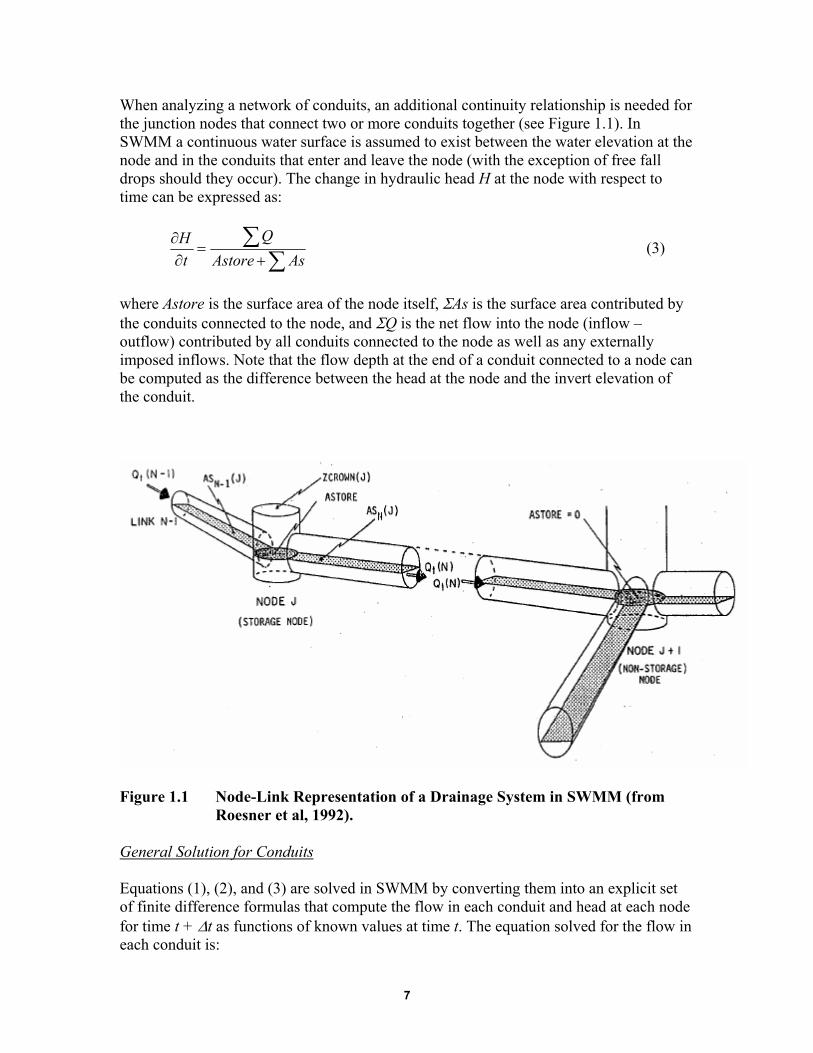


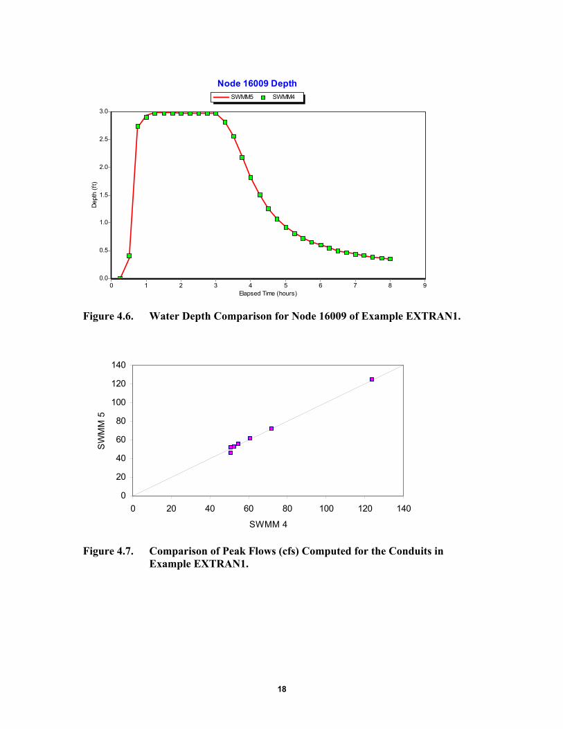
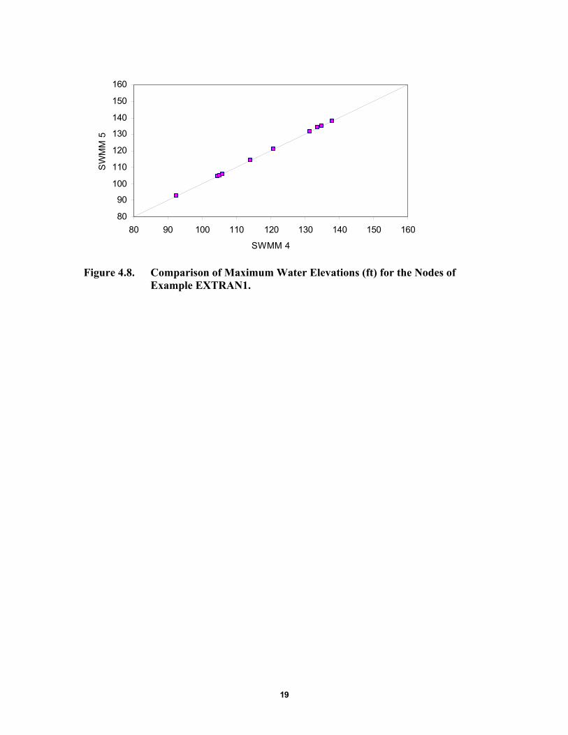


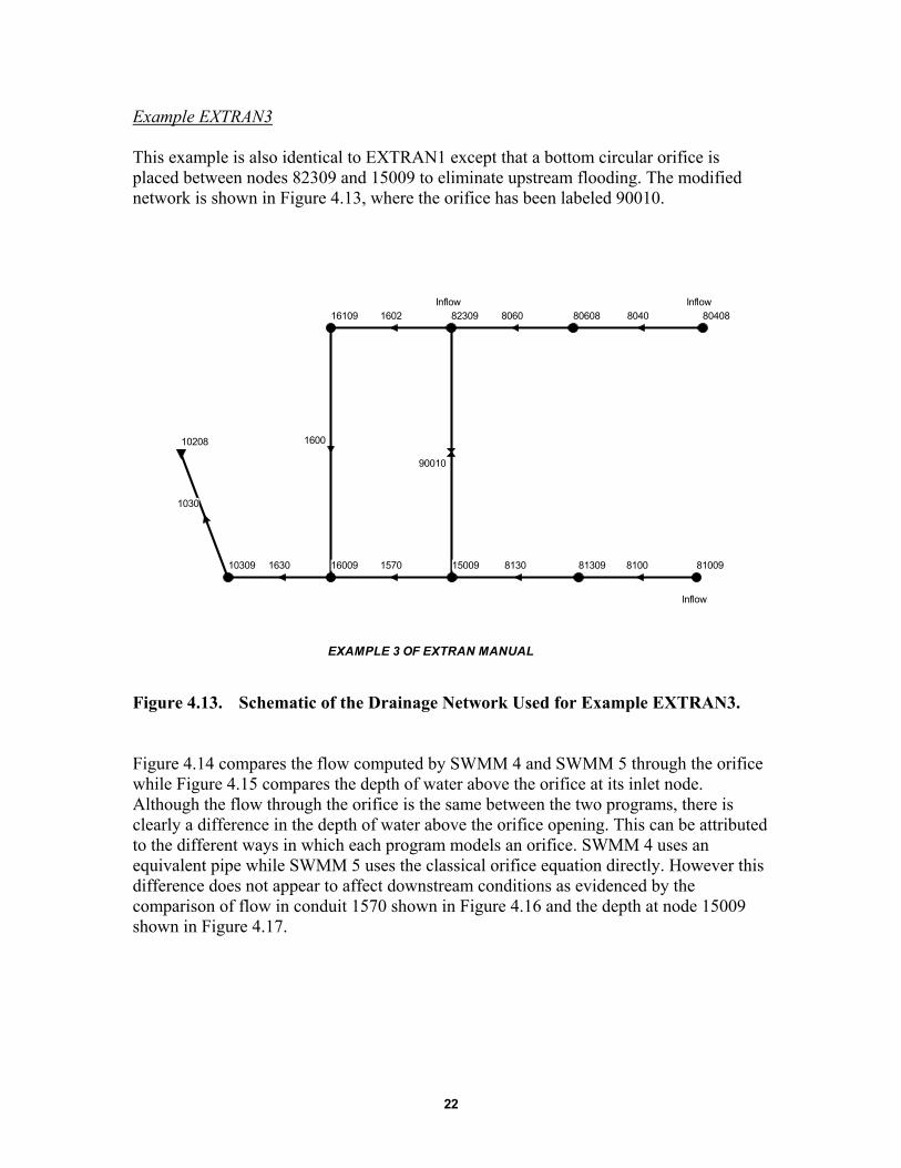
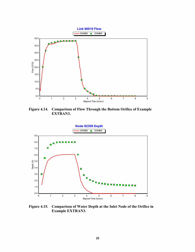


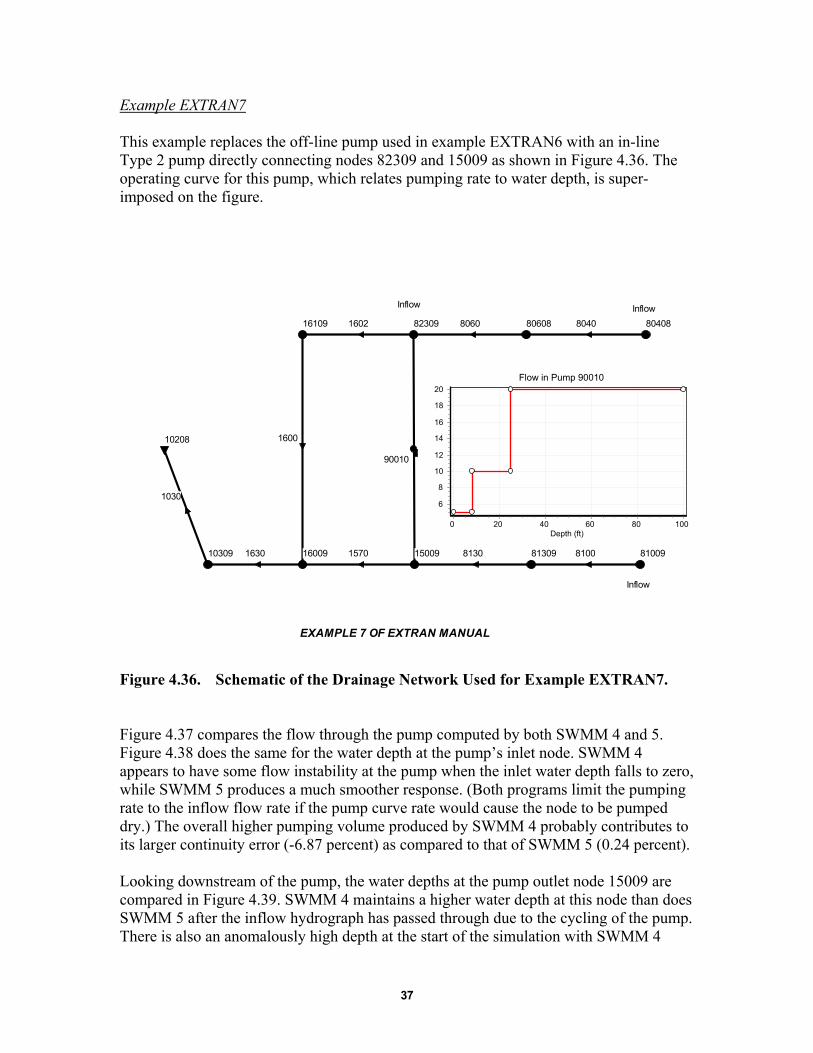


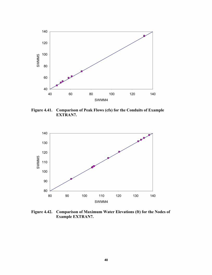


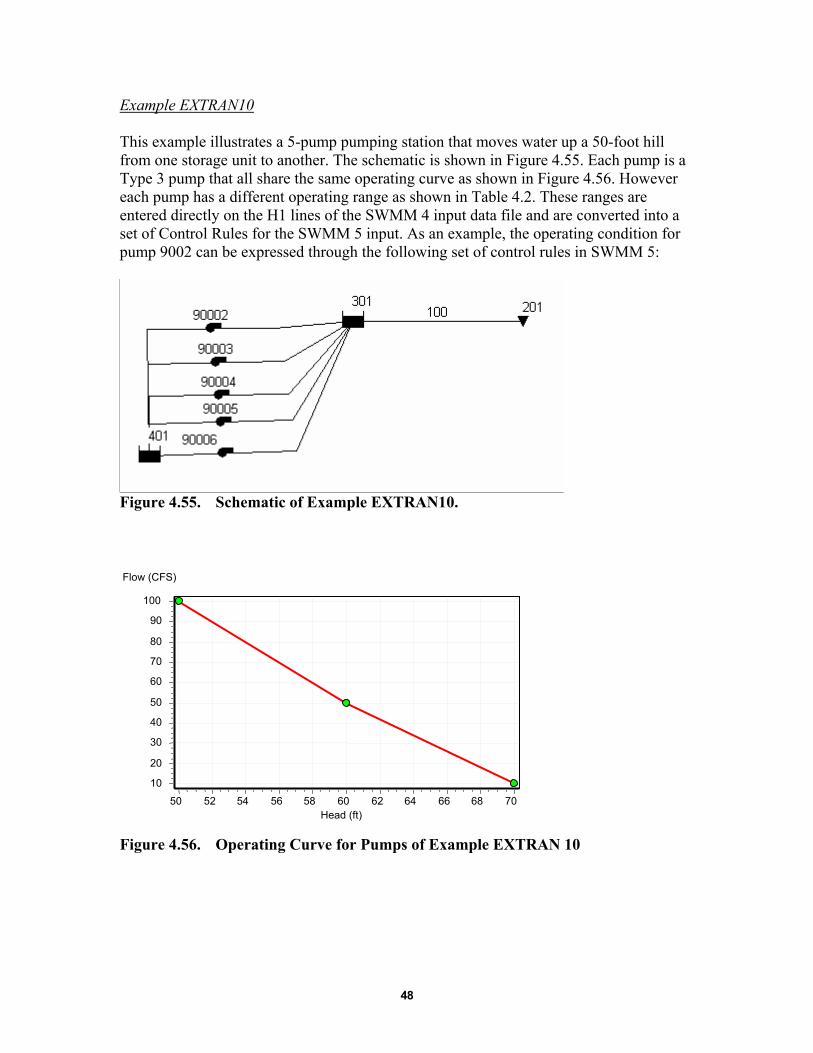
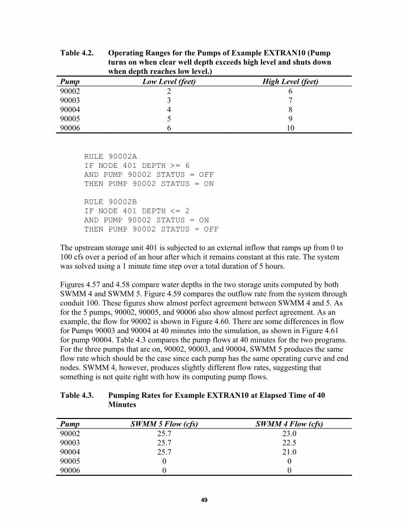

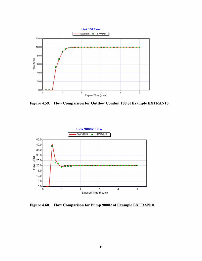
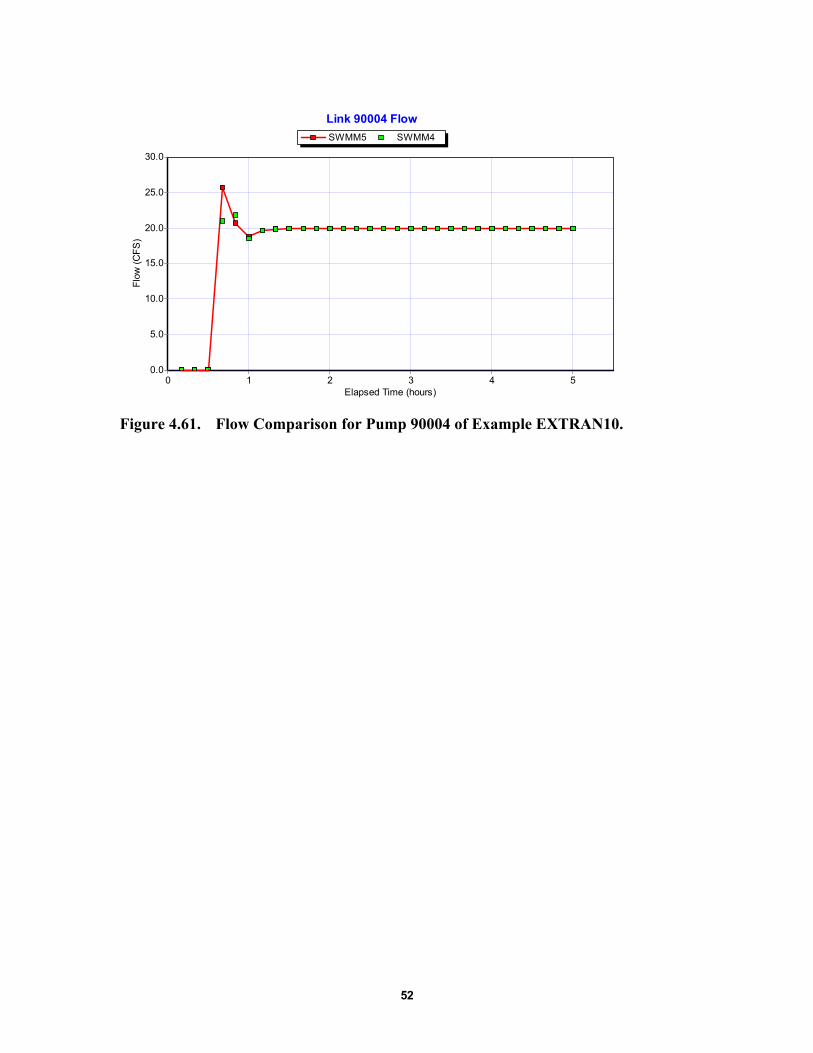


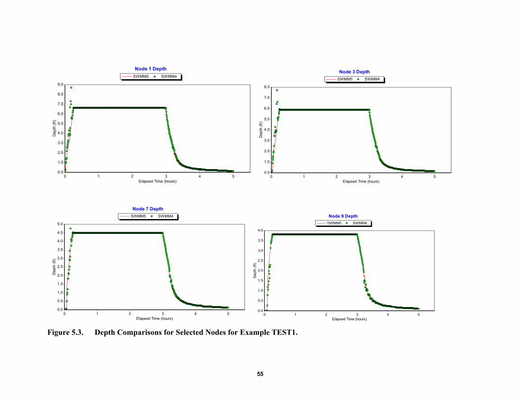


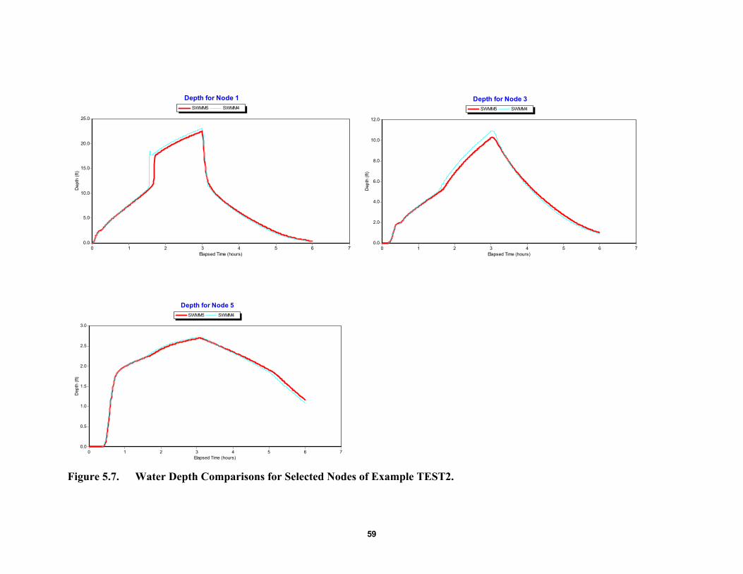


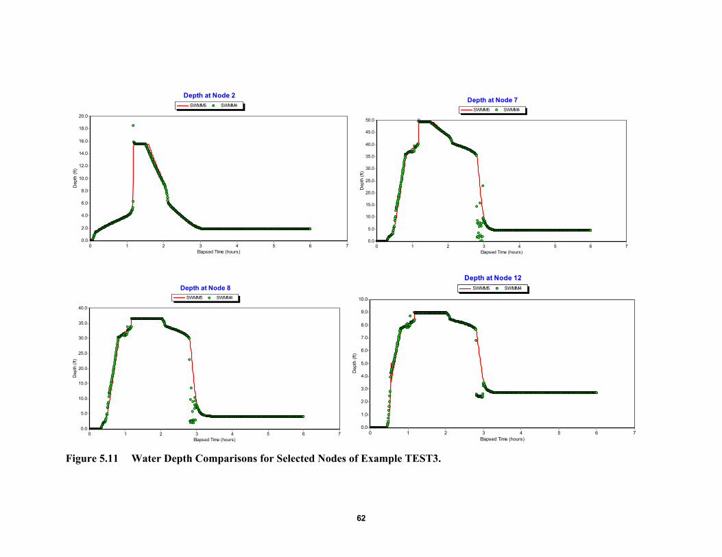


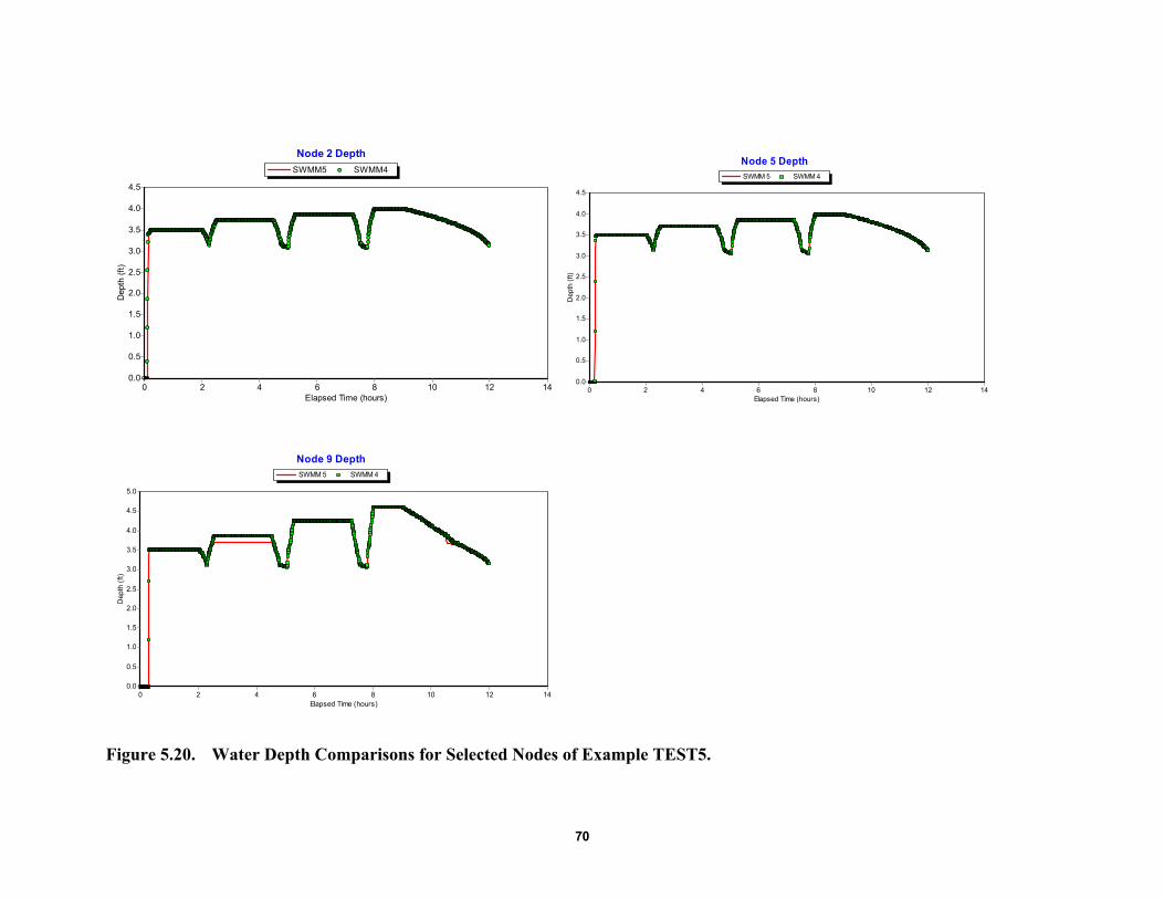


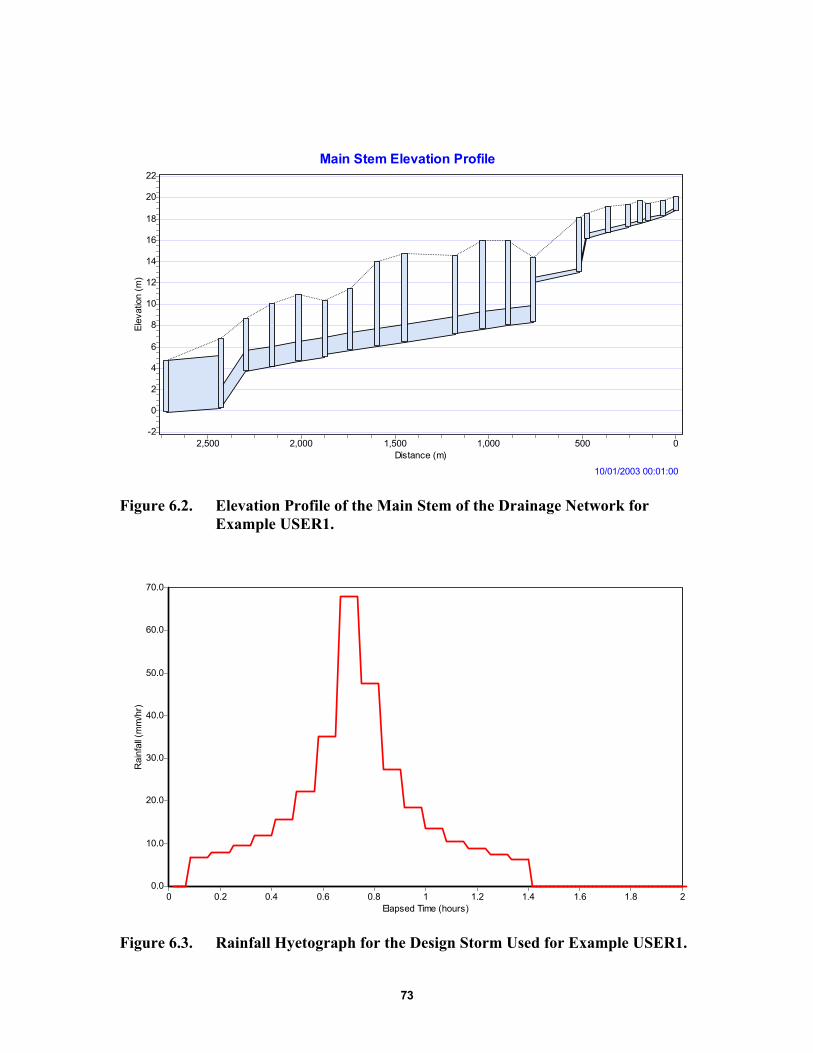


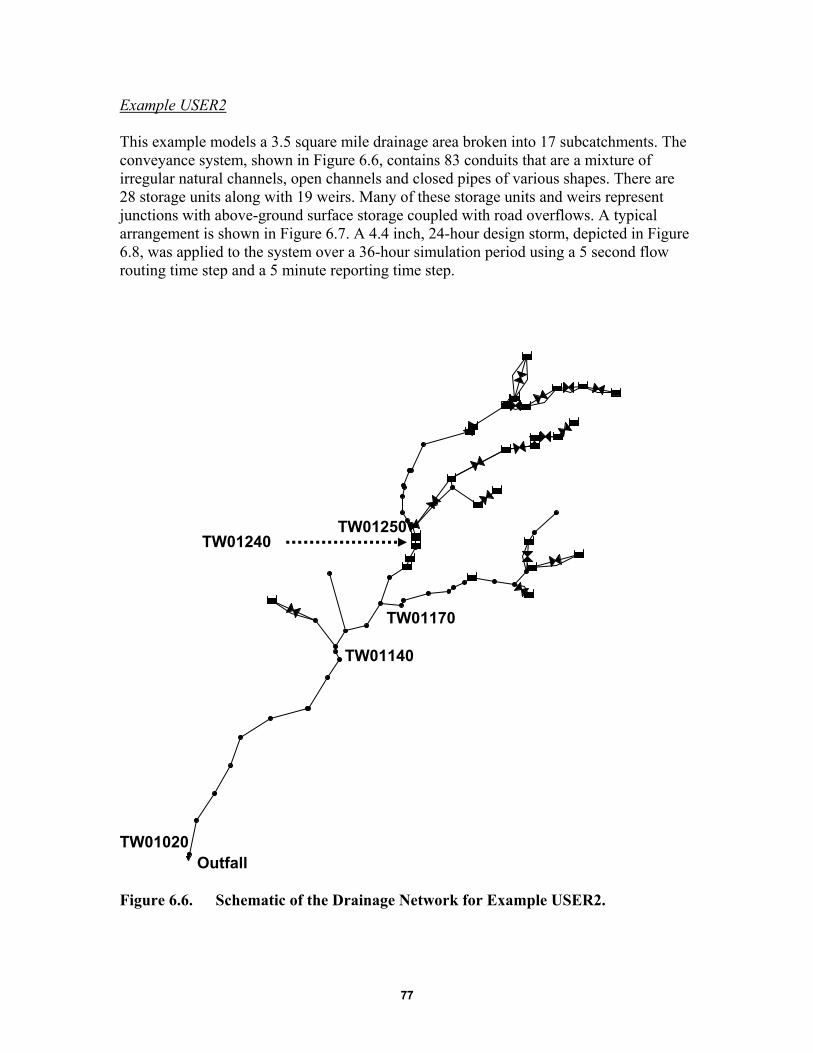


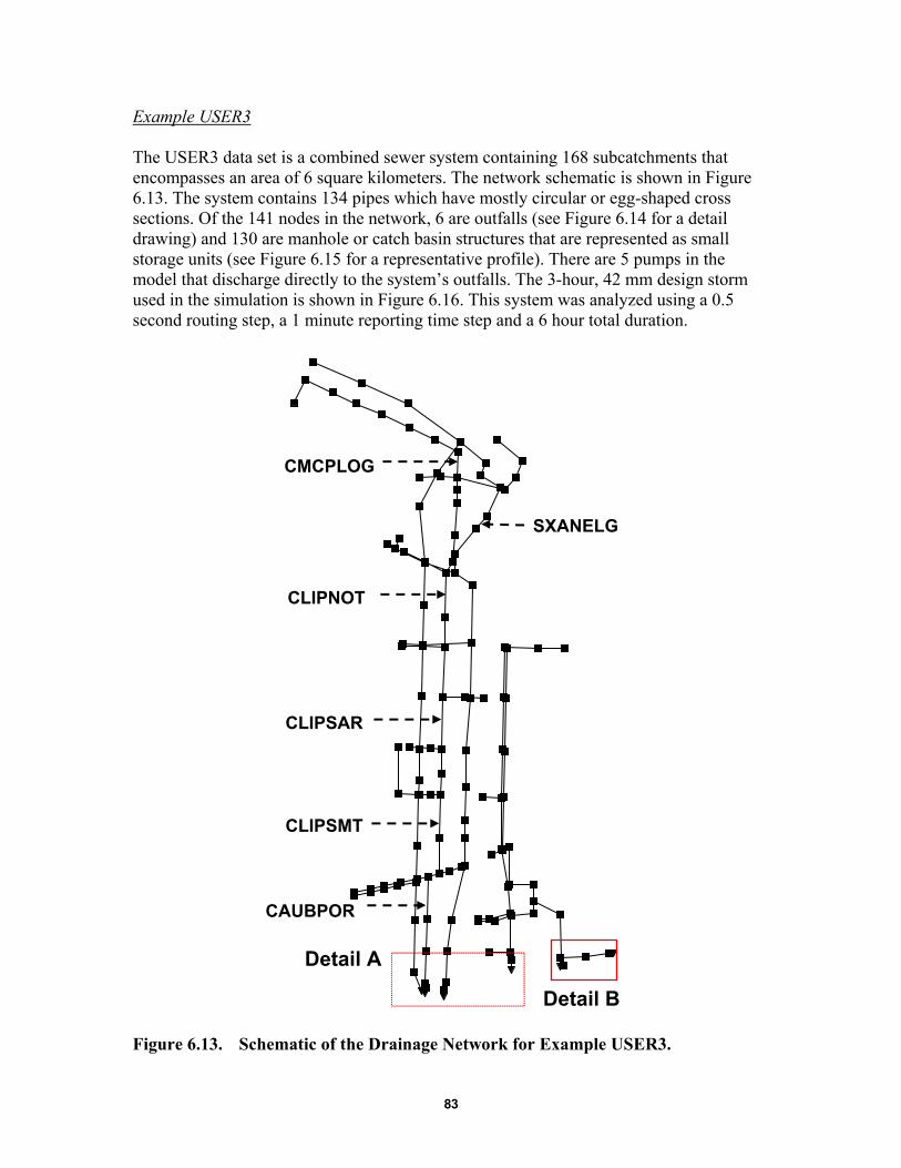
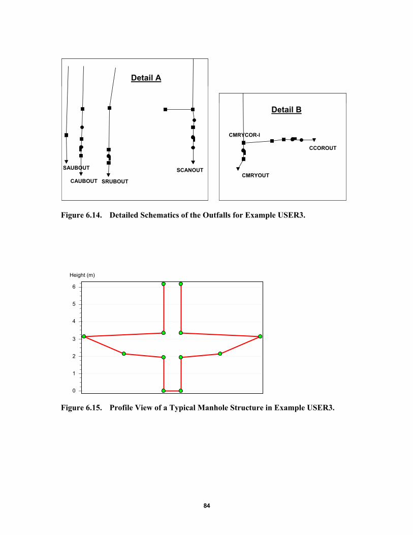
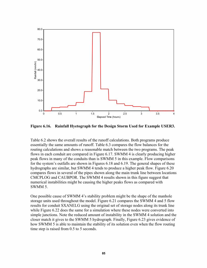


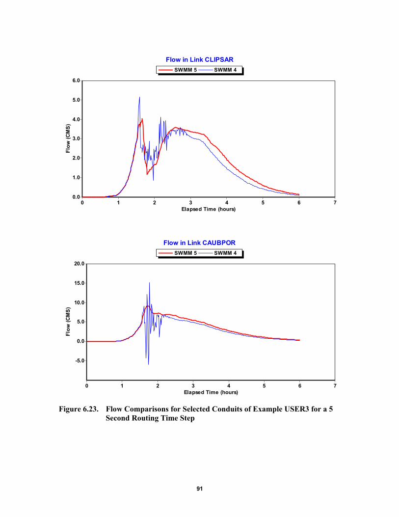
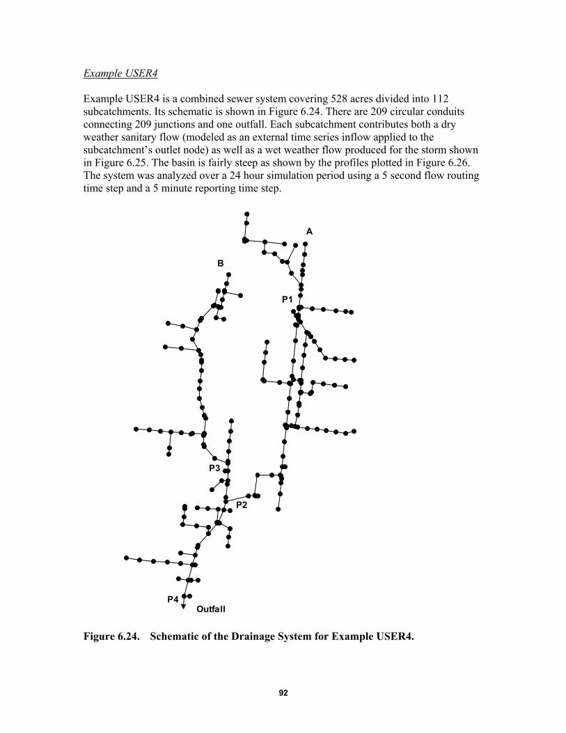
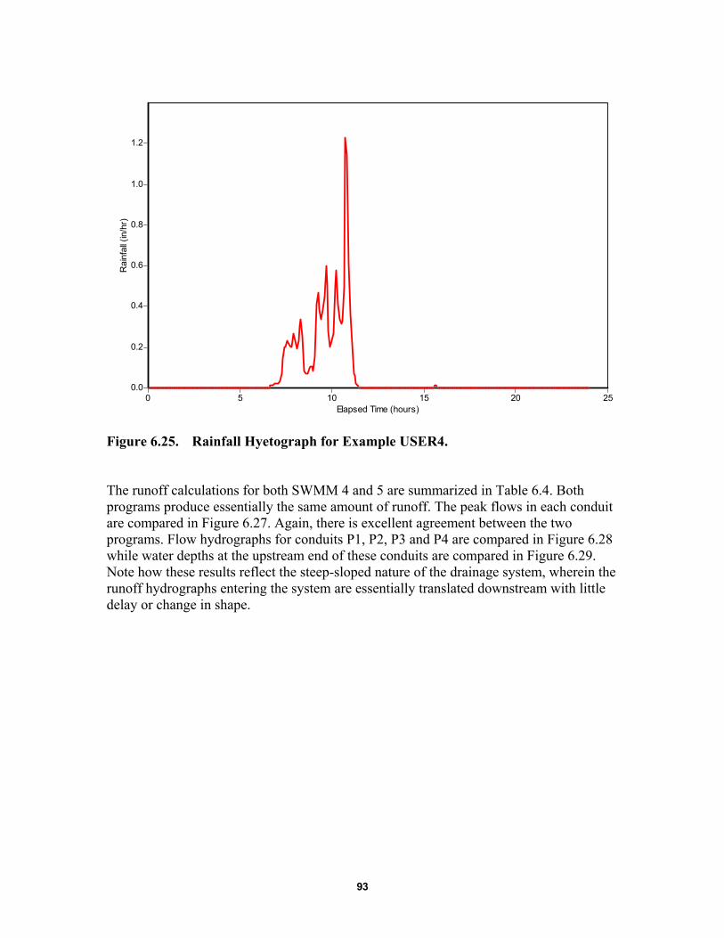
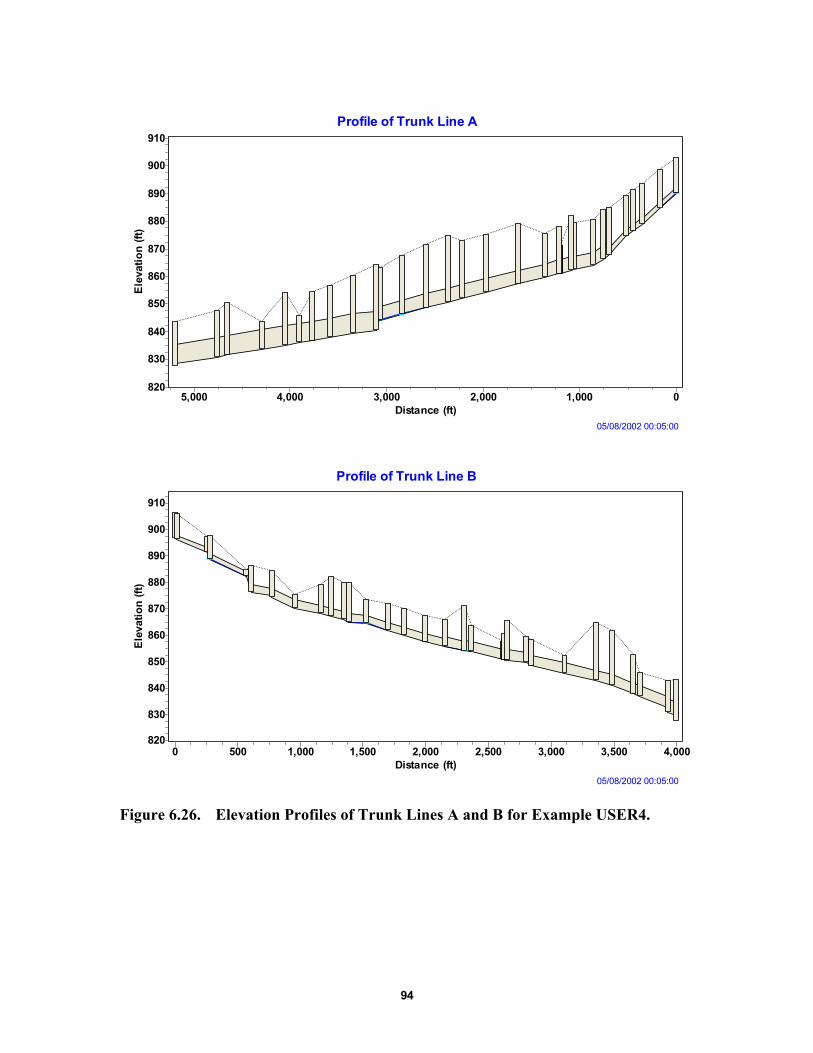


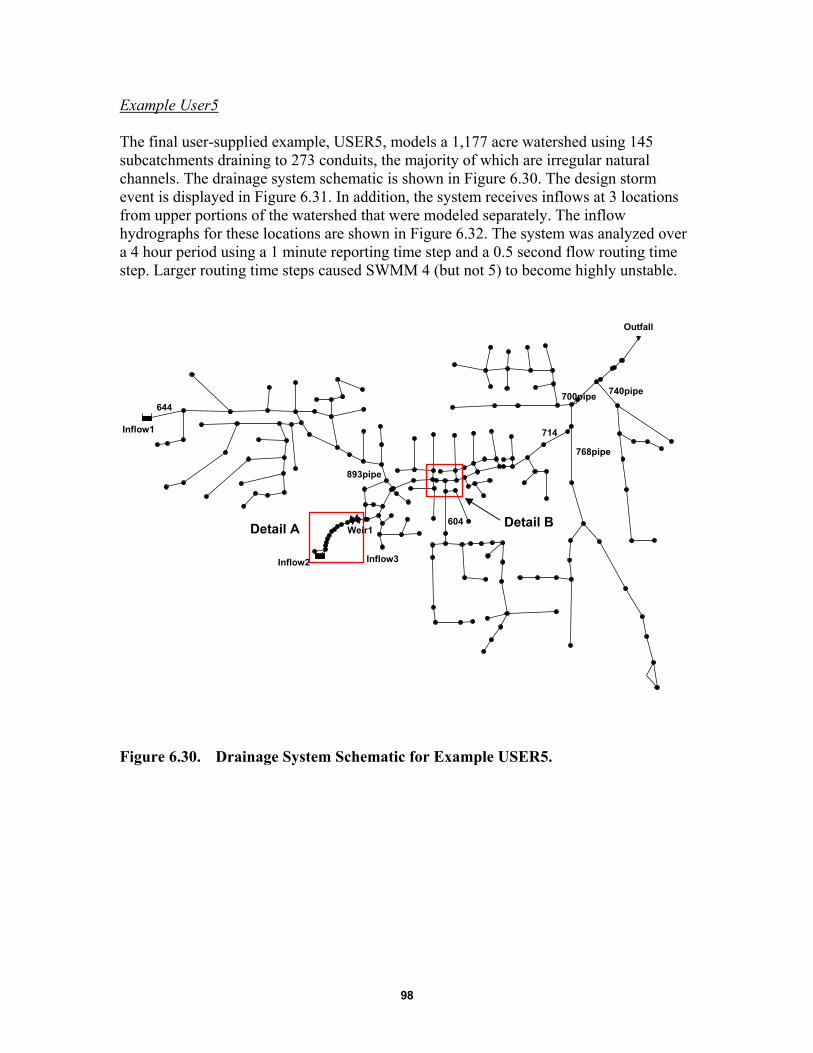
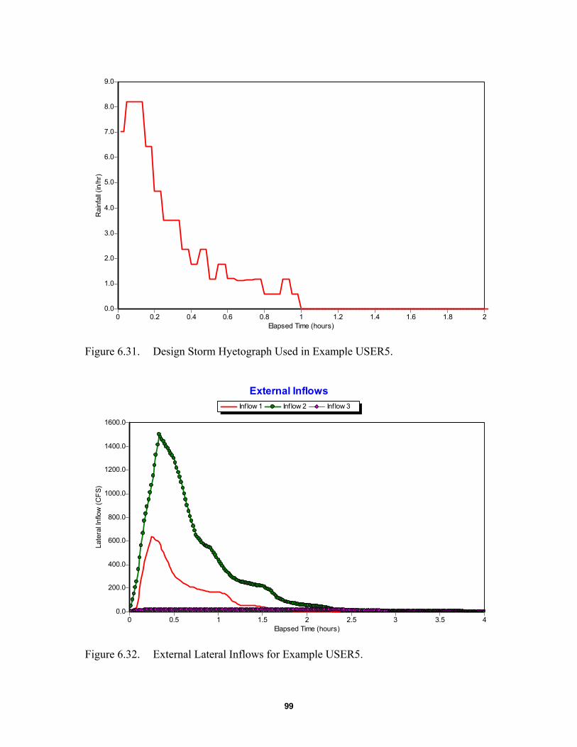


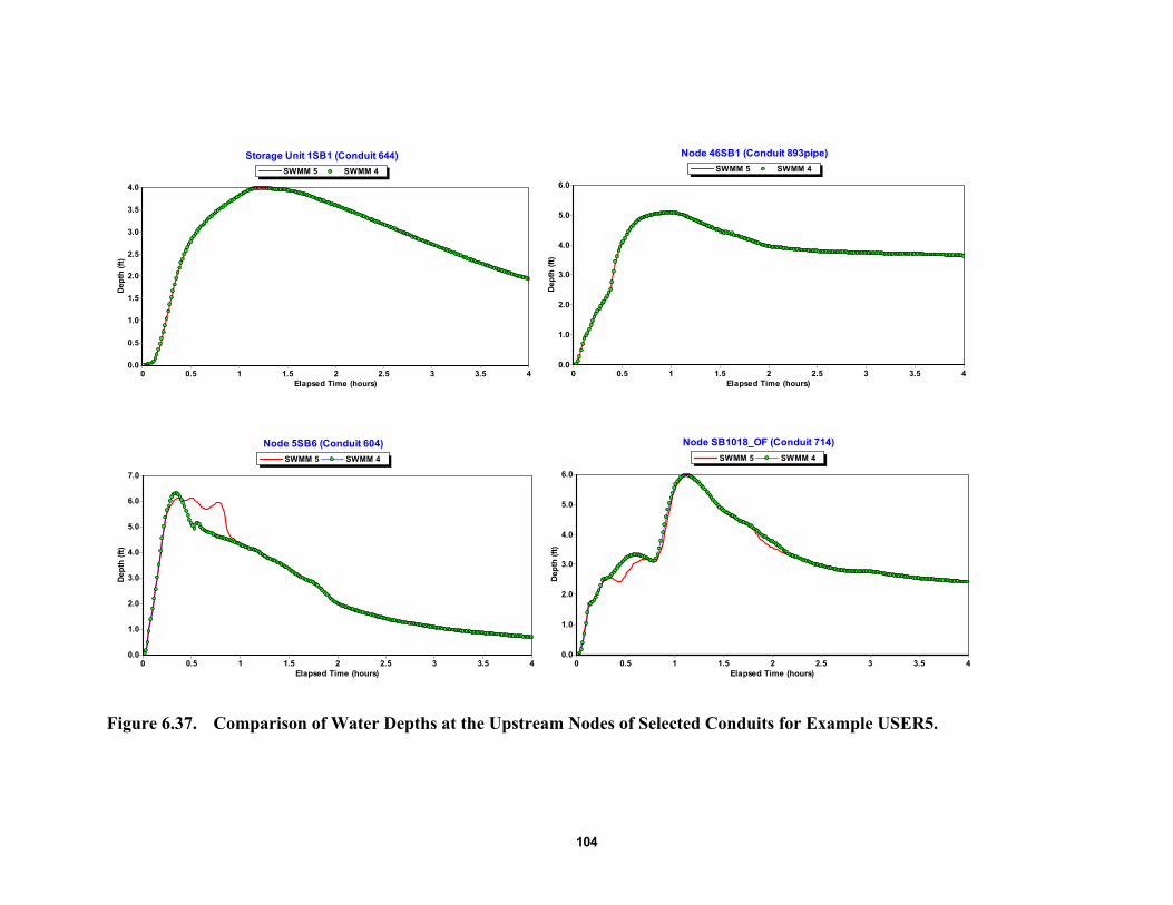

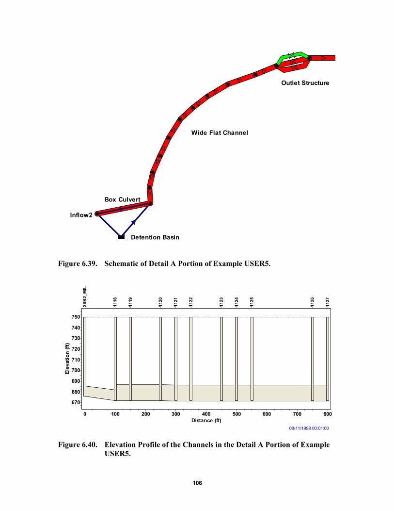


![[List University Name] Quality Assurance Program ... Assurance Foms/University... · [List University Name] Quality Assurance Program Description Document ... Quality Assurance Program](https://static.documents.pub/doc/80x56/5ab8c3d37f8b9aa6018d08ac/list-university-name-quality-assurance-program-assurance-fomsuniversitylist.jpg)