This paper was a Keynote Address at the Engineering Conferences International Conference on Urban Runoff Modeling: Intelligent Modeling to Improve Stormwater Management, Humboldt State Univ., Arcata, CA, July 2007. Stormwater Runoff Modeling; Is it as Accurate as We Think? Ben Urbonas, P.E., D.WRE 1 ABSTRACT Multi-million if not multi-billion dollar decisions are being made on the basis of computer modeling results. The question that is often not explored is how reliable and accurate are these results? This paper explores several issues related to modeling using distributed rainfall-runoff models as they may affect accuracy and reliability of results. Issues such as continuous simulation, design storms, temporal and spatial rainfall data density in continuous simulations, aerial corrections for modeling larger catchments and others are discussed and challenges to the modeler community are posed. In addition, this paper presents a brief history of past Engineering Foundation Conferences (currently under the ECI banner) sponsored by the Urban Water Resources Research Council of the American Society of Civil Engineers (currently part of the Environment and Water Resources Institute of ASCE). Introduction Multi-million if not multi-billion dollar decisions are being made on the basis of computer modeling results. The question that is often not explored is how reliable and accurate are these results? This paper explores many of the issues related to the accuracy of modeling. It does represents a point of view of a part-time software developer, user of software and reviewer of many computer modeling runs dealing with hydrology and hydraulics. The points of view and observations expressed have also been shaded through working with a significant number of rainfall-runoff data sets since 1977. Accurate and reliable modeling of stormwater runoff (i.e., hydrology) and associated phenomena has been in the past and continues today to be a challenge. This is despite the vast advances in the models themselves, their interfaces and even their math engines. What we have now are a wide array of products that have great user interfaces and input/output management systems, making their use by less and less skilled professionals a current reality. Most of the distribute rainfall-runoff models still rely on calibration to achieve an accurate representation of the hydrology they model. However, much less than five percent of all the hydrologic simulation in the United States (off the cuff estimate/guess by the author based on observation over the last 30+ years) has simultaneous rainfall-runoff data to calibrate against. Even when such data are available, it may not have sufficient time of record and may not be of sufficient temporal or spatial density. What I have observed time and time again is the pursuit of precision with little concern for accuracy. The big question that I raise to the leading professionals and model builders is: Is it possible to guide the user to achieve accuracy and 1 Manager, Master Planning Program, Urban Drainage and Flood Control District, Denver, Colorado 1 Urbonas
Transcript
This paper was a Keynote Address at the Engineering Conferences International Conference on Urban Runoff Modeling: Intelligent Modeling to Improve Stormwater Management, Humboldt State Univ., Arcata, CA, July 2007.
Stormwater Runoff Modeling; Is it as Accurate as We Think?
Ben Urbonas, P.E., D.WRE 1 ABSTRACT Multi-million if not multi-billion dollar decisions are being made on the basis of computer modeling results. The question that is often not explored is how reliable and accurate are these results? This paper explores several issues related to modeling using distributed rainfall-runoff models as they may affect accuracy and reliability of results. Issues such as continuous simulation, design storms, temporal and spatial rainfall data density in continuous simulations, aerial corrections for modeling larger catchments and others are discussed and challenges to the modeler community are posed.
In addition, this paper presents a brief history of past Engineering Foundation Conferences (currently under the ECI banner) sponsored by the Urban Water Resources Research Council of the American Society of Civil Engineers (currently part of the Environment and Water Resources Institute of ASCE).
Introduction Multi-million if not multi-billion dollar decisions are being made on the basis of computer modeling results. The question that is often not explored is how reliable and accurate are these results? This paper explores many of the issues related to the accuracy of modeling. It does represents a point of view of a part-time software developer, user of software and reviewer of many computer modeling runs dealing with hydrology and hydraulics. The points of view and observations expressed have also been shaded through working with a significant number of rainfall-runoff data sets since 1977.
Accurate and reliable modeling of stormwater runoff (i.e., hydrology) and associated phenomena has been in the past and continues today to be a challenge. This is despite the vast advances in the models themselves, their interfaces and even their math engines. What we have now are a wide array of products that have great user interfaces and input/output management systems, making their use by less and less skilled professionals a current reality.
Most of the distribute rainfall-runoff models still rely on calibration to achieve an accurate representation of the hydrology they model. However, much less than five percent of all the hydrologic simulation in the United States (off the cuff estimate/guess by the author based on observation over the last 30+ years) has simultaneous rainfall-runoff data to calibrate against. Even when such data are available, it may not have sufficient time of record and may not be of sufficient temporal or spatial density. What I have observed time and time again is the pursuit of precision with little concern for accuracy. The big question that I raise to the leading professionals and model builders is: Is it possible to guide the user to achieve accuracy and 1 Manager, Master Planning Program, Urban Drainage and Flood Control District, Denver, Colorado
1 Urbonas
This paper was a Keynote Address at the Engineering Conferences International Conference on Urban Runoff Modeling: Intelligent Modeling to Improve Stormwater Management, Humboldt State Univ., Arcata, CA, July 2007.
deemphasize precision?
What are the most important elements in stormwater modeling? My personal observations and those of many of my colleagues agree on the following:
• The modeler’s skill is most important. • Selecting the appropriate model is next.
o Some models are best for urban areas dealing with small sub-catchments. o Others are best for large non-urban catchments. o What happens when we have a large urban catchment or mixed catchment?
• Next in importance is the math engine of model, provided, o It has no significant bugs o It represents the equations it uses accurately o It provides for user input to override defaults built into the code
Some of these issues and topics will be explored and possible challenges raised to the model developer and user communities.
Effects of Spatial Raingage Density When we do continuous simulations over extended periods of time we often have to use whatever rainfall data that are available though the National Weather Service. That data are collected almost never at the site being investigated and are only available in 1-hour and 15-minute clock time increments. We are very lucky if we get data at the analysis site itself and even luckier if we have more than one raingage at that site with a period of record exceeding three years.
USGS has been collecting simultaneous rainfall-runoff data at Harvard Gulch Catchment since 1980 for the Urban Drainage and Flood Control District (UDFCD) at 5-minute time increments during rainfall seasons of April through September. Unfortunately, because of computer system changes, USGS has lost access to this data prior to 1990 and only 15 years of 5-minute rainfall and flow data were available.
The Harvard Gulch catchment has a 3.1 square mile area, which is mostly covered by single family residential neighborhoods, but it also has significant areas of very dense commercial development and several small parks. This catchment has two continuous flow gages and five continuous raingages. On occasion a raingage was out of operation, and to maintain continuous record, the data from the closest raingage was used to fill out its record. This occurred in less than 2% of the storm events between 1990 and 2005.
An EPA SWMM model in kinematic mode was set up for this catchment. It was divided into 59 sub-catchments along the lines of similar land uses and developments (see Figure 1). The levels of impervious cover and drainage systems were field and aerial photo verified. All of these runoff elements were linked with routing elements, mostly open channel and several storm sewers. Each element was set up to have an overflow when its initial design capacity was exceeded, routing the flows to streets or adjacent floodplains. It was calibrated to match peaks and volumes for a number of recorded events (see Figure 2).The calibrated model was then used to test the effects of raingage special density and the effects of temporal data density.
For testing the spatial density the data from one, two, three, four and five rain gages were used and compared to the calibrated five gage modeled runoff peaks and volumes and against the recorded peaks and volumes. Tables 1 and 2 compare peaks for two different scenarios of gage placement against the 5-gage calibrated model and against the recorded flows. The trends seen under Denver rainfall conditions were relatively clear. A raingage density of approximately one gage per square mile is needed to achieve most accurate results.
2 Urbonas
This paper was a Keynote Address at the Engineering Conferences International Conference on Urban Runoff Modeling: Intelligent Modeling to Improve Stormwater Management, Humboldt State Univ., Arcata, CA, July 2007.
Figure 1. Harvard Gulch monitored catchment
Perfect Fit LineR2 = 0.9449
0.000
0.050
0.100
0.150
0.200
0.250
0.300
0.350
0.400
0 0.1 0.2 0.3 0.4
Observed Runoff Volume - Inches
Best Regression FitR2 = 0.94
0.0
100.0
200.0
300.0
400.0
500.0
600.0
700.0
800.0
0 100 200 300 400 500 600 700 800
Observed Peak Flows - CFS
Figure 2. Calibration results for peaks (left) and volumes (right)
Other observations include that if only one raingage is to be used, locating it near the centroid of this 3.1 sq. mi. catchment gave the most accurate results and if two gages were used, placing them at the opposite ends of the catchment gave the best results. Regardless, the accuracy of continuous simulations can significantly be affected by lack of sufficient raingage density or even the lack of raingages in the modeled catchments. As a result, the trends developed on the basis of continuous simulations are, at best, approximations. Ones that have to be questioned if they are any better than using well thought-out and region-specific design storms when judging the sufficiency of the existing conveyance systems or the sizing for new ones. This is especially of concern when calibration data are not even available.
3 Urbonas
This paper was a Keynote Address at the Engineering Conferences International Conference on Urban Runoff Modeling: Intelligent Modeling to Improve Stormwater Management, Humboldt State Univ., Arcata, CA, July 2007.
Table 1. Peak flow variances for raingage densities vs. 5-gage modeled peaks.
Table 2. Peak flow variances for raingage densities vs. recorded flows.
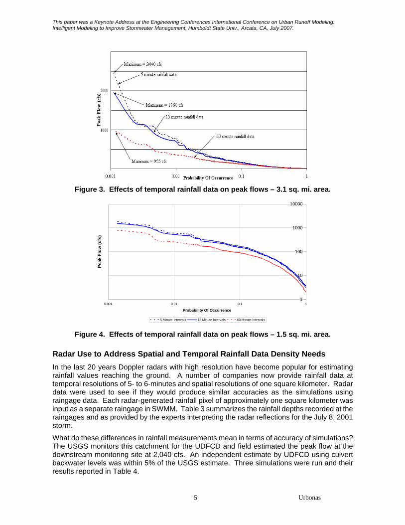
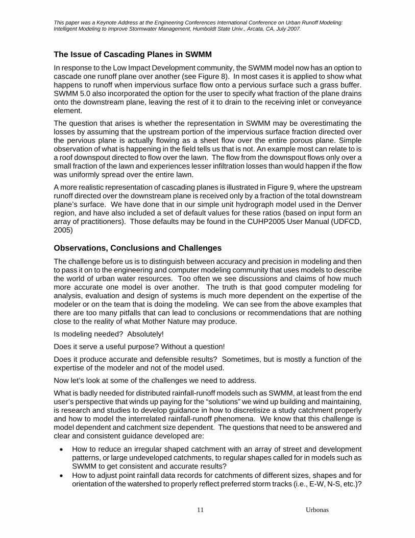
Effects of Temporal Rainfall Data Density Using the same calibrated catchment model the effects of temporal density were also tested. The 5-minute data for all five gages were agglomerated into 15-minute and 60-minute data based on clock time. The effects on the peak flows can be seen in Figures 3 for the full 3.1 square mile catchment simulations and in Figure 4 for a 1.3 square mile portion of the simulation.
The differences in peak flows between the 5-minute and the 15-minute data are noticeable but not that significant. However, when comparing the results from the 5-minute to 60-minute data we see the simulated peak flows differ by a factor of two. Similar, but not quite as severe differences were found for the runoff volumes.
Clearly, if we are to achieve a credible level of accuracy in urban runoff simulations, we need rainfall data at no greater than 15-minute increments, preferably 5-minute increments. This observation may not be so distinct in regions where rainfall patterns are very uniform and of lower intensities, such as in the Pacific Northwest.
4 Urbonas
This paper was a Keynote Address at the Engineering Conferences International Conference on Urban Runoff Modeling: Intelligent Modeling to Improve Stormwater Management, Humboldt State Univ., Arcata, CA, July 2007.
Figure 3. Effects of temporal rainfall data on peak flows – 3.1 sq. mi. area.
Figure 4. Effects of temporal rainfall data on peak flows – 1.5 sq. mi. area.
Radar Use to Address Spatial and Temporal Rainfall Data Density Needs In the last 20 years Doppler radars with high resolution have become popular for estimating rainfall values reaching the ground. A number of companies now provide rainfall data at temporal resolutions of 5- to 6-minutes and spatial resolutions of one square kilometer. Radar data were used to see if they would produce similar accuracies as the simulations using raingage data. Each radar-generated rainfall pixel of approximately one square kilometer was input as a separate raingage in SWMM. Table 3 summarizes the rainfall depths recorded at the raingages and as provided by the experts interpreting the radar reflections for the July 8, 2001 storm.
What do these differences in rainfall measurements mean in terms of accuracy of simulations? The USGS monitors this catchment for the UDFCD and field estimated the peak flow at the downstream monitoring site at 2,040 cfs. An independent estimate by UDFCD using culvert backwater levels was within 5% of the USGS estimate. Three simulations were run and their results reported in Table 4.
5 Urbonas
This paper was a Keynote Address at the Engineering Conferences International Conference on Urban Runoff Modeling: Intelligent Modeling to Improve Stormwater Management, Humboldt State Univ., Arcata, CA, July 2007.
Table 3. Comparison recorded rainfall totals vs. radar-generated totals for the July 8, 2001 storm at Harvard Gulch catchment.
Rain Gage Location Radar Raingage inches percentLogan Street 2.13 1.34 0.79 59Harvard Park 2.62 1.20 1.42 118Slaven Elementary 3.89 1.35 2.54 188University Park School 3.89 4.48 -0.59 -13Jackson Street (Colo Blvd) 4.08 2.48 1.60 65Bethesda Center 2.83 2.97 -0.14 -5Bradley Elementary 2.59 2.42 0.17 7
AVERAGE 0.83 60
DifferenceRainfall Depth-inchesy
Table 4. Simulation of July 8, 2001 Storm using three rainfall inputs.
Modeling Rainfall Data Scenario Model Results Difference from Field Estimate
Using 5-min data from 5 Rain-Gages 2,140 cfs +5% Using 5-min Radar-Generated Rain 3,250 cfs +59% Using 80% of 5-min Radar Rain 2,220 cfs +9%
Clearly the use of radar-generated rainfall data in this case grossly overestimated the runoff rates during this storm event. The data had to be reduced by 20% to bring in the simulated peak flow to within 10% of the field estimate.
Use of Models with Suspect Calibration Data Verification of Flow Measurements by USGS When calibration data are available, what is almost always not being asked is how accurate are the data. For the Harvard Gulch catchment the data delivered originally some 15 years ago by USGS were tested for consistency. Initial comparisons of runoff volumes for lower (at Harvard Park) and upper (at Colorado Blvd) catchment flow gages against rainfall volumes were performed. Harvard Gulch at Harvard Park and Harvard Gulch at Colorado catchments were found to have runoff coefficients of 0.15 and 0.34 respectively. The upper catchment had a coefficient that appeared to be within a reasonable range for the land uses within it. The gage at Harvard Park had a coefficient that was clearly too low for the land uses within its catchment. This prompted us to evaluate the validity of the flow gage-rating curve at this location. We filed surveyed 16 channel cross-sections within a 850-foot reach.
Each of the cross-sections was divided into 4 to 5 sections for which Manning’s n values were derived at different stages of flow based on retardance curves for the vegetative ground cover at each of the sections. New depth-flow rating curves were then developed using multiples of HEC-2 runs. What evolved were a set of equations that were used to modify the original USGS data. The resultant runoff-to-rainfall ratio was approximately 0.25, which was judged to be much more representative than the 0.15 obtained using uncorrected flow data. Since then, USGS has conducted its own flow-rating studies at the Harvard Gulch site and the data received since then appear to be reasonable when compared to the rainfall volumes for each of the events.
Lesson learned, never use rainfall-runoff data for calibration without checking it for integrity and reasonableness. This may appear as a trivial recommendation, but the author is aware of one
6 Urbonas
This paper was a Keynote Address at the Engineering Conferences International Conference on Urban Runoff Modeling: Intelligent Modeling to Improve Stormwater Management, Humboldt State Univ., Arcata, CA, July 2007.
PhD thesis that was based on flow data that were found by UDFCD to result in significantly more runoff volume than rainfall. Something that we in the West would love to have, but mother nature seems to have other ideas.
Use of an Uncalibrated Models Shortly after the modeling of radar-generated rainfall data at the Harvard Gulch catchment, a separate runoff model was set up independently by a consultant working for the City and County of Denver to help Denver assess their drainage system needs. They used local criteria without any calibration, a practice that is typical for most of the storm system analysis and design throughout the United States. We ran their model using the July 8, 2001 rainfall raingage and radar-generated rainfall data. The following table summarizes the comparisons between the field estimates, calibrated model peak flow estimates and the consultant’s model results using the two sets of rainfall data:
Table 4. Simulations of July 8, 2001 Storm using uncalibrated model as compared to the calibrated model and field data.
Peak Flow source Peak Flow % Difference from Field Estimate
Field estimate peak flow 2,040 cfs Using calibrated SWMM w/ 5 gages 2,140 cfs +5% Using project’s uncalibrated model: w/ 5-rain-gage record 5,780 cfs +180% w/ 80% radar-generated rainfall 5,330 cfs 160% w/ 100% radar-generated rainfall 7,090 cfs +250%
This illustrates that the blind use of off-the-shelf models and published standards can lead to costly mistakes in analysis and design. However, most urban catchments do not have data to calibrate with and often the engineer falls back on local criteria and blind use of it without much thought if the results make any sense or have any relation to realities observed in the field. Putting it another way, it is not the model but the modeler that can make the greatest difference in whether the results are reliable or not.
Blind Test of Models by UWRRC Nine uncalibrated rainfall-runoff models were tested under the sponsorship of the ASCE Urban Water Resources Research Council in the mid-1990s using data from two gaged sites. The rainfall data and catchment parameter data were provided to volunteers experienced with each of the models – CASC2D, CUHP, CUHP/SWM, DR3M, HEC-1 (KW option), HSPF, PSRM, EPA SWMM, and TR20 by Phillip Zarriello of USGS Ithaca, NY office. The resultant finding for the peak flows and how they compared against the measured peaks for each of the events at the two sites are presented in Figure 5 (Zarriello, 1998). Unfortunately the TR20 results are not shown on these graphs, but its simulations consistently underestimated the peak flows by a factor or about 50% or more. What this illustrates is that uncalibrated models can either be on target or can be off by a very large factor for the recorded peak flows. The level of errors varied between the two sites amongst the models as well.
7 Urbonas
This paper was a Keynote Address at the Engineering Conferences International Conference on Urban Runoff Modeling: Intelligent Modeling to Improve Stormwater Management, Humboldt State Univ., Arcata, CA, July 2007.
Figure 5. Results of blind test simulated vs. recorded peak flows using Harvard Gulch
in Denver, CO and Surry Downs in Bellevue, WA data.
Spatial Variability of Rainfall and Modeling Accuracy When we use the often maligned Design Storm, we have guidance (i.e., NOAA Atlas) for the correction of storm depths with increasing catchment area. However, we found this guidance to be inappropriate for the semi-arid climate of Colorado’s High Plains and its mountains. It appears that the spatial variability and aerial coverage by rainstorms in this region for convective storms average approximately 2-square miles and an elongated footprint. Nevertheless, the use of design storms with NOAA aerial correction guidance is the currently accepted state-of-practice, appropriate or not.
8 Urbonas
This paper was a Keynote Address at the Engineering Conferences International Conference on Urban Runoff Modeling: Intelligent Modeling to Improve Stormwater Management, Humboldt State Univ., Arcata, CA, July 2007.
At the same time, there is no credible guidance for adjusting storm depths or footprints when simulating runoff with increasing catchments area. As a result, accuracy of simulated results for larger catchments is highly questionable and it is clear that the use of point rainfall data that assumes it is falling uniformly over entire catchments is inappropriate except for very small catchments.
To further illustrate this point, Figure 6 summarized the analysis of runoff data at 18 sites (no rainfall data at these sites) in the Denver region. It is something we were not able to replicate using computer modeling. What this figure reveals is that the peak flows per square mile drop off with increasing catchment area, clearly identifying the effects of rainfall aerial footprint sizes and distributions.
52.4%40.2%
46.5%43.3%
33.3%
15.5%
18.0%
55.4%
24.3%
46.1%39.1%
10.1%
60.9%26.8%
29.8%
0
100
200
300
400
500
600
700
800
900
1000
0 2 4 6 8 10
TRIBUTARY AREA (SQUARE MILES)
FLO
W (C
FS)
12
Imp. = 40%
Imp. = 30%
Imp. = 20%
Imp. = 60%
Figure 6. Two-year peak flows based on analysis of peak flow data at 18 sites.
Uncertainties Resulting from Rainfall Data Length of Record Figure 7 illustrates the mean, 5% and 95% confidence bands for the mean when the continuous simulation peak flows are processed using Log Pearson Type 3 flow frequency analysis using annual duration series (i.e., annual peaks) for the 15 years of record simulation results using the 5-raingage data set for Harvard Gulch. Note how the means for the pre- and post-developed catchment conditions overlap past the 10-year return periods. What is even more interesting is how the uncertainty of the mean increases with the return period to a point where the mean loses any sense of credibility at higher return periods. Keep in mind that this was done using a calibrated model with high spatial and temporal density of rainfall data. Can we really claim that continuous simulation is more accurate than the use of a design storm for predicting flooding levels at return periods the 5-year storm and larger for this site?
9 Urbonas
This paper was a Keynote Address at the Engineering Conferences International Conference on Urban Runoff Modeling: Intelligent Modeling to Improve Stormwater Management, Humboldt State Univ., Arcata, CA, July 2007.
Figure 7. Peak flow and confidence limits vs. return period at Harvard Gulch.
Figure 8. Cascading planes as represented in EPA SWMM.
Unconnected Impervious
Separate Pervious
Receiving Pervious
Connected Impervious
Figure 9. Possibly a more realistic representation of cascading planes.
10 Urbonas
This paper was a Keynote Address at the Engineering Conferences International Conference on Urban Runoff Modeling: Intelligent Modeling to Improve Stormwater Management, Humboldt State Univ., Arcata, CA, July 2007.
The Issue of Cascading Planes in SWMM In response to the Low Impact Development community, the SWMM model now has an option to cascade one runoff plane over another (see Figure 8). In most cases it is applied to show what happens to runoff when impervious surface flow onto a pervious surface such a grass buffer. SWMM 5.0 also incorporated the option for the user to specify what fraction of the plane drains onto the downstream plane, leaving the rest of it to drain to the receiving inlet or conveyance element.
The question that arises is whether the representation in SWMM may be overestimating the losses by assuming that the upstream portion of the impervious surface fraction directed over the pervious plane is actually flowing as a sheet flow over the entire porous plane. Simple observation of what is happening in the field tells us that is not. An example most can relate to is a roof downspout directed to flow over the lawn. The flow from the downspout flows only over a small fraction of the lawn and experiences lesser infiltration losses than would happen if the flow was uniformly spread over the entire lawn.
A more realistic representation of cascading planes is illustrated in Figure 9, where the upstream runoff directed over the downstream plane is received only by a fraction of the total downstream plane’s surface. We have done that in our simple unit hydrograph model used in the Denver region, and have also included a set of default values for these ratios (based on input form an array of practitioners). Those defaults may be found in the CUHP2005 User Manual (UDFCD, 2005)
Observations, Conclusions and Challenges The challenge before us is to distinguish between accuracy and precision in modeling and then to pass it on to the engineering and computer modeling community that uses models to describe the world of urban water resources. Too often we see discussions and claims of how much more accurate one model is over another. The truth is that good computer modeling for analysis, evaluation and design of systems is much more dependent on the expertise of the modeler or on the team that is doing the modeling. We can see from the above examples that there are too many pitfalls that can lead to conclusions or recommendations that are nothing close to the reality of what Mother Nature may produce.
Is modeling needed? Absolutely!
Does it serve a useful purpose? Without a question!
Does it produce accurate and defensible results? Sometimes, but is mostly a function of the expertise of the modeler and not of the model used.
Now let’s look at some of the challenges we need to address.
What is badly needed for distributed rainfall-runoff models such as SWMM, at least from the end user’s perspective that winds up paying for the “solutions” we wind up building and maintaining, is research and studies to develop guidance in how to discretisize a study catchment properly and how to model the interrelated rainfall-runoff phenomena. We know that this challenge is model dependent and catchment size dependent. The questions that need to be answered and clear and consistent guidance developed are:
• How to reduce an irregular shaped catchment with an array of street and development patterns, or large undeveloped catchments, to regular shapes called for in models such as SWMM to get consistent and accurate results?
• How to adjust point rainfall data records for catchments of different sizes, shapes and for orientation of the watershed to properly reflect preferred storm tracks (i.e., E-W, N-S, etc.)?
11 Urbonas
This paper was a Keynote Address at the Engineering Conferences International Conference on Urban Runoff Modeling: Intelligent Modeling to Improve Stormwater Management, Humboldt State Univ., Arcata, CA, July 2007.
12 Urbonas
• How to properly apply cascading planes in SWMM and other models? • Which models are most appropriate and inappropriate for use in urban areas? • How to develop robust guidance for model users to produce more reliable and more
accurate answers when calibration data are not available (this is the case in well over 95% of all drainage and water quality studies being conducted today)?
• Should users arbitrarily discard the design storm approach for analysis and design in favor of continuous simulation when we have not yet answered the above-stated needs and shortcomings of recorded storms and their blind application without adequate accurate rainfall-runoff data for calibration?
In addition, we need to:
• Continue research to develop robust tools to convert radar images to accurate rainfall depths on the ground at high spatial and temporal resolutions.
• Pursue the Weather Service for production of much longer records (25-year of data at the minimum) of temporally denser rainfall data (i.e., 5-minute and 15-minute) for all of their first order weather stations.
• Modify EPA SWMM to allow for varying the receiving porous area fraction that receives the cascading impervious fraction.
• Continue to develop guidance in how to develop design storms that give realistic representation of runoff rates and volumes for the return periods (i.e., 1-, 2-, 5-, 10-year, etc.) along with appropriate antecedent precipitation requirements for each.
References Zarriello, P. J. (1998). “Comparison of Nine Uncalibrated Runoff Models to Observed Flows in
Two Small Urban Catchments,” Proceedings First Federal Interagency Hydrology Model Conference, Las Vegas, NV, April, 1998: Subcommittee on Hydrology of Interagency Advisory Committee on Water Data, p. 7–163 to 7-170.
UDFCD (2005). Colorado Urban Hydrograph Procedure Excel-Based Computer Program – User Manual, Urban Drainage and Flood Control District.